Embed Size (px)
Citation preview

Impact of partial and imperfect testing on reliability assessment of safety instrumented systemsPossible approaches for inclusion of its
effects in reliability assessments
Eleojo Samuel Ocheni
Reliability, Availability, Maintainability and Safety (RAMS)
Supervisor: Mary Ann Lundteigen, IPK
Department of Production and Quality Engineering
Submission date: June 2015
Norwegian University of Science and Technology

RAMSReliability, Availability,
Maintainability, and Safety
Impact of partial and imperfect testing on
reliability assessment of safety instrumented
systems.
Ocheni, Eleojo Samuel
June 2015
MASTER THESIS
Department of Production and Quality Engineering
Norwegian University of Science and Technology
Supervisor: Professor Mary Ann Lundteigen
Co-Supervisor: Fares Innal

i
Preface
This master’s thesis is written during 20 weeks throughout spring 2015 as a fulfilment of one of
the prerequisites for the award of master’s degree (MSc) in Reliability, Availability, Maintainabil-
ity and Safety, at the Norwegian University of Science and Technology. This thesis with title ’Im-
pact of partial and imperfect testing on reliability assessment of safety instrumented systems’ is
written with the guidance of my supervisor professor Mary Ann Lundteigen and co-supervisor
Fares Innal at the department of reliability, availability, maintainability and safety (RAMS), fac-
ulty of Production and Quality Engineering.
The reader of this thesis is assumed to have some basic knowledge within the field of reli-
ability and should be familiar with the textbook System Reliability Theory: Models, Statistical
Methods, and Applications by Rausand and Høyland. Familiarity with the IEC 61508 standard is
also key to understanding this work.
I would like to thank my supervisor, Mary Ann Lundteigen for her help, guidance and sup-
port with this project. Further thanks to my co-supervisor Fares Innal for his important feedback
and input throughout this thesis.
Trondheim, 2015-06-10
Ocheni, Eleojo Samuel

ii
Acknowledgment
My special thanks goes to my supervisor, Professor Mary Ann Lundteigen for the support and
mentoring during this project. Her patience, encouragement and coaching has made it possible
for the realization of this thesis. I would also like to thank Fares Innal for his unflinching sup-
port and contribution throughout this thesis. His guidance with the use of the GRIF software is
remarkable.
Finally, I would like to thank my parents, siblings and friends for their moral and psycholog-
ical support during this period.
Ocheni E. S.
iii
Summary and Conclusions
Testing of safety instrumented systems is vital to ensure they are able to perform the required
safety function when the need arises. These tests are carried out at specified time intervals. The
verification of the ability of the safety systems to perform as required is carried out by reliability
assessment. This is the calculation of how likely it is that the safety instrumented system will
function when needed.
In carrying out reliability assessment, proof testing of safety systems is assumed to be per-
fect which is not always the case in reality. This thesis is important because it looks at how to
evaluate this assumption to achieve a realistic estimate since testing is a key factor in reliability
calculation. This study identifies the main causes of imperfectness which are classified with the
five M-factors namely: Method, Machine, Manpower, Milieu and Material. Based on these, the
situations where perfect test may not be realistic with examples are reviewed and documented.
I have studied and compared different ways that the effects of tests can be treated. Three
approaches to consider imperfectness of test were identified: the IEC 61508 approach where
we consider the proportion (fraction) of dangerous undetected failures that are revealed by the
proof test, the probability of detecting a dangerous undetected failure during a given proof test
and the PDS method of adding a constant probability of test independent failures. The anal-
ysis carried out compared the first and second approach. Based on the analysis, the second
approach was proposed to be the most suitable of the first two approaches.
Furthermore, we present different reliability assessment methods for estimating the prob-
ability of failure on demand of a safety system. The methods used are: analytical formulas,
multi-phase Markov, fault tree approach and Petri net. The principles of application and limi-
tation with each of these approaches are presented in this thesis. In the course of this work, we
discovered that some complicated cases and systems can only be analyzed by simulation. Fi-
nally, a chemical reactor protection system is used as a case study to demonstrate the principles
and methods discussed in this thesis.
Contents
Preface . . . . . . . . . . . . . . . . . . . . . . . . . . . . . . . . . . . . . . . . . . . . . . . . i
Acknowledgment . . . . . . . . . . . . . . . . . . . . . . . . . . . . . . . . . . . . . . . . . . ii
Summary and Conclusions . . . . . . . . . . . . . . . . . . . . . . . . . . . . . . . . . . . . iii
1 Introduction 2
1.1 Background . . . . . . . . . . . . . . . . . . . . . . . . . . . . . . . . . . . . . . . . . . 2
1.2 Problem situation . . . . . . . . . . . . . . . . . . . . . . . . . . . . . . . . . . . . . . . 3
1.3 Objective . . . . . . . . . . . . . . . . . . . . . . . . . . . . . . . . . . . . . . . . . . . . 4
1.4 Study approach . . . . . . . . . . . . . . . . . . . . . . . . . . . . . . . . . . . . . . . . 4
1.5 Limitation . . . . . . . . . . . . . . . . . . . . . . . . . . . . . . . . . . . . . . . . . . . 5
1.6 Structure of report . . . . . . . . . . . . . . . . . . . . . . . . . . . . . . . . . . . . . . 5
2 Failure classification and testing Concepts 7
2.1 Failure classification . . . . . . . . . . . . . . . . . . . . . . . . . . . . . . . . . . . . . 7
2.1.1 Common Cause Failures (CCF) . . . . . . . . . . . . . . . . . . . . . . . . . . . 10
2.1.2 Influence of Common Cause Failures on testing . . . . . . . . . . . . . . . . . 10
2.2 Principles of testing . . . . . . . . . . . . . . . . . . . . . . . . . . . . . . . . . . . . . . 11
2.2.1 Proof test/Function test . . . . . . . . . . . . . . . . . . . . . . . . . . . . . . . 11
2.2.2 Perfect test and Imperfect testing . . . . . . . . . . . . . . . . . . . . . . . . . 12
2.2.3 Reasons for having imperfect test . . . . . . . . . . . . . . . . . . . . . . . . . 13
2.2.4 Online and offline testing . . . . . . . . . . . . . . . . . . . . . . . . . . . . . . 15
2.2.5 Full proof test and partial test . . . . . . . . . . . . . . . . . . . . . . . . . . . . 16
2.3 Partial Stroke Testing . . . . . . . . . . . . . . . . . . . . . . . . . . . . . . . . . . . . . 17
2.3.1 Determining the PST coverage . . . . . . . . . . . . . . . . . . . . . . . . . . . 19
iv
CONTENTS v
2.4 Relationship between the types of tests . . . . . . . . . . . . . . . . . . . . . . . . . . 21
2.5 Adverse effects of full proof testing and partial testing . . . . . . . . . . . . . . . . . 22
2.6 Test strategies . . . . . . . . . . . . . . . . . . . . . . . . . . . . . . . . . . . . . . . . . 22
3 Analytical formulas for performance of SIS 24
3.1 Analytical approach based on full proof tests . . . . . . . . . . . . . . . . . . . . . . . 24
3.1.1 IEC 61508 approach . . . . . . . . . . . . . . . . . . . . . . . . . . . . . . . . . 24
3.1.2 ISA approach . . . . . . . . . . . . . . . . . . . . . . . . . . . . . . . . . . . . . 26
3.1.3 The PDS method . . . . . . . . . . . . . . . . . . . . . . . . . . . . . . . . . . . 27
3.1.4 Other authors approaches . . . . . . . . . . . . . . . . . . . . . . . . . . . . . . 28
3.1.5 Summary on the different analytical formulas . . . . . . . . . . . . . . . . . . 31
4 Partial and Imperfect testing 32
4.1 Analytical formulas for imperfect testing . . . . . . . . . . . . . . . . . . . . . . . . . 32
4.2 IEC 61508 approach . . . . . . . . . . . . . . . . . . . . . . . . . . . . . . . . . . . . . 33
4.3 PDS method . . . . . . . . . . . . . . . . . . . . . . . . . . . . . . . . . . . . . . . . . . 34
4.3.1 Probability of Test Independent Failures . . . . . . . . . . . . . . . . . . . . . 35
4.3.2 Incorporating PTC into PFD Formulas . . . . . . . . . . . . . . . . . . . . . . 36
4.3.3 Discussion on the use of PTC and PT I F . . . . . . . . . . . . . . . . . . . . . . 37
4.4 The Markovian approach to partial testing . . . . . . . . . . . . . . . . . . . . . . . . 38
4.5 Other authors approaches to partial tests . . . . . . . . . . . . . . . . . . . . . . . . . 41
4.6 Partial tests impact on PFD calculation . . . . . . . . . . . . . . . . . . . . . . . . . . 43
5 Verification of Analytical formulas for testing 45
5.1 Phased Markov for periodically tested components . . . . . . . . . . . . . . . . . . . 45
5.1.1 Application of multi-phase Markov by analysis of a 1oo1 system . . . . . . . 46
5.1.2 Multi-phase Markov result comparison with partial test consideration . . . 49
5.1.3 Limitation of the Markov approach . . . . . . . . . . . . . . . . . . . . . . . . 51
5.2 Use of Fault tree . . . . . . . . . . . . . . . . . . . . . . . . . . . . . . . . . . . . . . . . 51
5.2.1 Fault tree result comparison with the partial test model . . . . . . . . . . . . 54
CONTENTS vi
6 Petri Net 56
6.1 Introduction to Petri Nets . . . . . . . . . . . . . . . . . . . . . . . . . . . . . . . . . . 56
6.1.1 Concepts of Petri nets . . . . . . . . . . . . . . . . . . . . . . . . . . . . . . . . 56
6.1.2 Petri net models for selected cases . . . . . . . . . . . . . . . . . . . . . . . . . 57
6.2 Combining elements behavior with Petri net . . . . . . . . . . . . . . . . . . . . . . . 63
6.2.1 Proper combining . . . . . . . . . . . . . . . . . . . . . . . . . . . . . . . . . . 63
6.2.2 Staggered test . . . . . . . . . . . . . . . . . . . . . . . . . . . . . . . . . . . . . 64
6.2.3 Common cause failures (CCF) contribution . . . . . . . . . . . . . . . . . . . 65
7 Case study 68
7.1 Chemical reactor protection system (CRPS) . . . . . . . . . . . . . . . . . . . . . . . 68
7.1.1 System description . . . . . . . . . . . . . . . . . . . . . . . . . . . . . . . . . . 68
7.1.2 Comparison and discussion of results . . . . . . . . . . . . . . . . . . . . . . . 69
8 Discussion and Conclusion 75
8.1 Discussion . . . . . . . . . . . . . . . . . . . . . . . . . . . . . . . . . . . . . . . . . . . 75
8.2 Conclusion . . . . . . . . . . . . . . . . . . . . . . . . . . . . . . . . . . . . . . . . . . . 76
8.3 Recommendations for further work . . . . . . . . . . . . . . . . . . . . . . . . . . . . 77
Bibliography 78
A Acronyms 82
B Fault tree of the case study 83
B.1 General part of the fault tree of the case study . . . . . . . . . . . . . . . . . . . . . . 83
B.2 Fault tree for independent failures of the FC . . . . . . . . . . . . . . . . . . . . . . . 83
B.3 Fault tree of CCF for the final control (FC) element . . . . . . . . . . . . . . . . . . . 83
C Petri net model of the case study 87
D The use of MAPLE software 89
List of Figures
2.1 Failure classification by causes (adapted from Hauge et al., 2013). . . . . . . . . . . 8
2.2 Classification of failure mode . . . . . . . . . . . . . . . . . . . . . . . . . . . . . . . . 9
2.3 Fishbone diagram for causes of imperfect testing (adapted from Rolén, 2007). . . . 14
2.4 Pressure transmitter test illustration . . . . . . . . . . . . . . . . . . . . . . . . . . . 15
2.5 Test apparatus for gas detectors . . . . . . . . . . . . . . . . . . . . . . . . . . . . . . 16
2.6 PST setup for integrated and separate vendor activation (adapted from Lundteigen
and Rausand, 2008a). . . . . . . . . . . . . . . . . . . . . . . . . . . . . . . . . . . . . . 17
2.7 Relevant failure rates (adapted from Lundteigen and Rausand, 2007). . . . . . . . . 18
2.8 Impact of PST on PFD (adapted from Lundteigen and Rausand, 2008a). . . . . . . . 19
2.9 Proof test classification (adapted from Rausand, 2014). . . . . . . . . . . . . . . . . . 21
3.1 Subsystem structure . . . . . . . . . . . . . . . . . . . . . . . . . . . . . . . . . . . . . 24
3.2 1oo1 RBD . . . . . . . . . . . . . . . . . . . . . . . . . . . . . . . . . . . . . . . . . . . . 25
3.3 CMooN factors based on system voting logic (adapted from Hokstad and Corneliussen,
2004). . . . . . . . . . . . . . . . . . . . . . . . . . . . . . . . . . . . . . . . . . . . . . . 27
4.1 The PFD(t) of a channel with imperfect proof-testing (adapted from Rausand, 2014). 33
4.2 Loss of safety contributors (adapted from Hauge et al., 2013). . . . . . . . . . . . . . 35
4.3 Approximate Markov model for 1oo2 system based on multi-phase Markov. . . . . 38
4.4 Undetected failure sequences for 1oo2 system. . . . . . . . . . . . . . . . . . . . . . 39
4.5 RBD of any component of a system subjected to partial tests. . . . . . . . . . . . . . 41
4.6 RBD of a koon system subject to partial tests. (adapted from Jin and Rausand, 2014). 42
vii
LIST OF FIGURES viii
5.1 Principle of the multiphase Markovian modeling (adapted from IEC-61508, 2009)
part 6. . . . . . . . . . . . . . . . . . . . . . . . . . . . . . . . . . . . . . . . . . . . . . . 46
5.2 1oo1 Markov model for a periodically tested element. . . . . . . . . . . . . . . . . . 47
5.3 Principle of multi-phase Markov modeling. . . . . . . . . . . . . . . . . . . . . . . . . 47
5.4 Passage matrix at the (K +1) ·Ti . . . . . . . . . . . . . . . . . . . . . . . . . . . . . . . 48
5.5 Markov model for 1oo1 subject to PT and FT. . . . . . . . . . . . . . . . . . . . . . . . 50
5.6 Representation of settings from the GRIF Markov module . . . . . . . . . . . . . . . 51
5.7 System unavailability graph for 1oo1 Markov model. . . . . . . . . . . . . . . . . . . 52
5.8 Modeling concept using Fault Tree. . . . . . . . . . . . . . . . . . . . . . . . . . . . . 53
5.9 Fault tree for a 1oo2 system. . . . . . . . . . . . . . . . . . . . . . . . . . . . . . . . . . 54
5.10 Basic event setup properties in GRIF. . . . . . . . . . . . . . . . . . . . . . . . . . . . 55
6.1 A simple Petri Net showing the main graphical elements. . . . . . . . . . . . . . . . 57
6.2 A Petri Net model for a failed and repaired component. . . . . . . . . . . . . . . . . 58
6.3 A PN model with inclusion of repair resources. . . . . . . . . . . . . . . . . . . . . . . 59
6.4 PN model for a DU failure subject to testing. . . . . . . . . . . . . . . . . . . . . . . . 59
6.5 PN model for Non-instantaneous test time. . . . . . . . . . . . . . . . . . . . . . . . 60
6.6 PN model for availability consideration of component. . . . . . . . . . . . . . . . . . 61
6.7 A Petri Net model for both partial and full tests. . . . . . . . . . . . . . . . . . . . . . 62
6.8 A PN model with imperfect test as proportion of unrevealed failures. . . . . . . . . 63
6.9 A PN of imperfect test as probability of not revealing failures. . . . . . . . . . . . . . 64
6.10 A PN model with probability of test induced failure. . . . . . . . . . . . . . . . . . . . 65
6.11 PN models for multiple components of different configurations. . . . . . . . . . . . 66
6.12 PN model for a uniformly distributed staggered tests. . . . . . . . . . . . . . . . . . . 66
6.13 PN model for CCF consideration. . . . . . . . . . . . . . . . . . . . . . . . . . . . . . . 67
7.1 High integrity protection system of a chemical reactor (CRPS) . . . . . . . . . . . . 69
7.2 CRPS reliability block diagram. . . . . . . . . . . . . . . . . . . . . . . . . . . . . . . . 69
7.3 PF D(t ) related to the imperfectness options: ξ= 0.7, σ= 0.7, λF T = 1E −6, τ= 1yr
and observation period of 10yr s. . . . . . . . . . . . . . . . . . . . . . . . . . . . . . . 72
7.4 PF D(t ) graph for uniformly distributed parameters with uncertainties. . . . . . . . 74
LIST OF FIGURES ix
B.1 General part of fault tree of the case study. . . . . . . . . . . . . . . . . . . . . . . . . 84
B.2 Fault tree for independent failures of the FC. . . . . . . . . . . . . . . . . . . . . . . . 85
B.3 Fault tree of CCF for the final control (FC) element. . . . . . . . . . . . . . . . . . . . 86
C.1 Part of PN model the CRPS system. . . . . . . . . . . . . . . . . . . . . . . . . . . . . 88
D.1 Formula generation using MAPLE . . . . . . . . . . . . . . . . . . . . . . . . . . . . . 90
List of Tables
3.1 Analytical formulas based on IEC 61508 . . . . . . . . . . . . . . . . . . . . . . . . . . 26
3.2 Analytical formulas based on ISA-TR84.00.02-2002 . . . . . . . . . . . . . . . . . . . 27
3.3 Analytical formulas based on PDS method (adapted from Hokstad and Corneliussen,
2004) . . . . . . . . . . . . . . . . . . . . . . . . . . . . . . . . . . . . . . . . . . . . . . 28
3.4 PDS simplified analytical formulas for PF Dav g of KooN architecture (adapted from
Hauge et al., 2013). . . . . . . . . . . . . . . . . . . . . . . . . . . . . . . . . . . . . . . 29
3.5 Selected configurations for formula by Oliveira and Abramovitch (2010) . . . . . . 30
3.6 Selected configurations for formula by Innal et al. (2015a) . . . . . . . . . . . . . . . 30
4.1 Formulas for PT I F for various voting logic (adapted from Hauge et al., 2013). . . . . 35
4.2 PF Dav g of selected configurations for Partial test formulas comparison . . . . . . 44
5.1 PF Dav g comparison of FTA and analytical formulas . . . . . . . . . . . . . . . . . . 55
7.1 Parameters for the system analysis . . . . . . . . . . . . . . . . . . . . . . . . . . . . . 70
7.2 Different cases with their related PF Dav g values by different methods . . . . . . . 71
1

Chapter 1
Introduction
Reliability is an important aspect of any engineering process. The use of safety instrumented
systems (SIS) to provide risk reduction of hazards to acceptable level, make operations safer
and more reliable. Testing of these SISs to ensure they are able to perform the intended function
when demand arises is therefore a necessity.
1.1 Background
Safety instrumented systems (SISs) are used in different industries to detect the onset of a haz-
ardous event and/or to mitigate the consequences. A SIS is made up of three subsystems namely
the input elements (sensors), the logic solver and the final (output) elements. The failure of a SIS
could lead to loss of lives, environmental disaster and damage of assets, therefore they should
be tested at time intervals to ensure they are able to perform the required safety function if a
demand arises. This explains why reliability assessments of SIS is of prominence starting from
the design to the operational phase, to ensure they meet a minimum functional specification.
Reliability assessments help to verify that the SIS is performing as required and as specified
in the safety requirement specification (SRS). A SIS may operate in low demand mode, high de-
mand mode or continuous mode. The probability of failure on demand (PFD) is used to assess
the safety integrity of SISs operating in low demand mode which is when the demand rate is less
than once per year. IEC 61508 and IEC 61511 are international standards that ensure functional
safety throughout the life cycle of a SIS. The IEC 61508 standard stipulates that SISs which are
2
CHAPTER 1. INTRODUCTION 3
operating in low demand mode could have some dangerous failures which are not detected by
the automatic diagnostic system (self-tests) therefore should be proof tested. The proof tests are
meant to reveal any dangerous undetected failures. Proof tests may be full or partial.
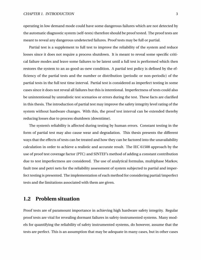
Partial test is a supplement to full test to improve the reliability of the system and reduce
losses since it does not require a process shutdown. It is meant to reveal some specific criti-
cal failure modes and leave some failures to be latent until a full test is performed which then
restores the system to an as-good-as-new condition. A partial test policy is defined by the ef-
ficiency of the partial tests and the number or distribution (periodic or non-periodic) of the
partial tests in the full test time interval. Partial test is considered as imperfect testing in some
cases since it does not reveal all failures but this is intentional. Imperfectness of tests could also
be unintentional by unrealistic test scenarios or errors during the test. These facts are clarified
in this thesis. The introduction of partial test may improve the safety integrity level rating of the
system without hardware changes. With this, the proof test interval can be extended thereby
reducing losses due to process shutdown (downtime).
The system’s reliability is affected during testing by human errors. Constant testing in the
form of partial test may also cause wear and degradation. This thesis presents the different
ways that the effects of tests can be treated and how they can be factored into the unavailability
calculation in order to achieve a realistic and accurate result. The IEC 61508 approach by the
use of proof test coverage factor (PTC) and SINTEF’s method of adding a constant contribution
due to test imperfectness are considered. The use of analytical formulas, multiphase Markov,
fault tree and petri nets for the reliability assessment of system subjected to partial and imper-
fect testing is presented. The implementation of each method for considering partial/imperfect
tests and the limitations associated with them are given.
1.2 Problem situation
Proof tests are of paramount importance in achieving high hardware safety integrity. Regular
proof tests are vital for revealing dormant failures in safety-instrumented systems. Many mod-
els for quantifying the reliability of safety instrumented systems, do however, assume that the
tests are perfect. This is an assumption that may be adequate in many cases, but in other cases
CHAPTER 1. INTRODUCTION 4
it may lead to overly optimistic estimates about the reliability performance since a proof test
differs from a real demand situation and some functions may be impossible to test due to po-
tential damage or wear out of the final elements. More focus is now directed to having realistic
rather than theoretical estimates of reliability, in particular from a safety barrier management
perspective. The question is "how can the imperfectness of tests be quantified or accounted for
in reliability assessment to have a more accurate estimate assuming that the tests are imper-
fect"?
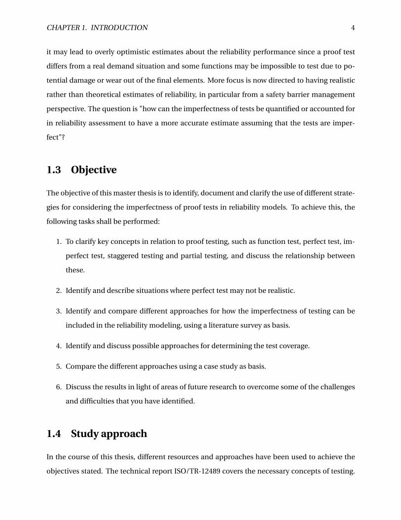
1.3 Objective
The objective of this master thesis is to identify, document and clarify the use of different strate-
gies for considering the imperfectness of proof tests in reliability models. To achieve this, the
following tasks shall be performed:
1. To clarify key concepts in relation to proof testing, such as function test, perfect test, im-
perfect test, staggered testing and partial testing, and discuss the relationship between
these.
2. Identify and describe situations where perfect test may not be realistic.
3. Identify and compare different approaches for how the imperfectness of testing can be
included in the reliability modeling, using a literature survey as basis.
4. Identify and discuss possible approaches for determining the test coverage.
5. Compare the different approaches using a case study as basis.
6. Discuss the results in light of areas of future research to overcome some of the challenges
and difficulties that you have identified.
1.4 Study approach
In the course of this thesis, different resources and approaches have been used to achieve the
objectives stated. The technical report ISO/TR-12489 covers the necessary concepts of testing.
CHAPTER 1. INTRODUCTION 5
The review of this report helps to gain the required knowledge and understanding associated
with testing. Imperfect testing in IEC 61508 (2009) and IEC 61511 (2014) standards is called non-
perfect proof test and very little about it is mentioned. The SINTEF’s PDS method handbook
(2006) has a different approach than the standards, making it interesting to study the different
approaches to imperfect testing. Discussions, inputs and recommendations from my supervi-
sors with both practical and theoretical testing experiences are also of great importance.
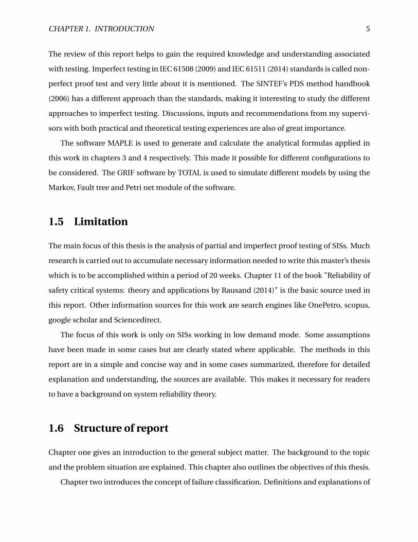
The software MAPLE is used to generate and calculate the analytical formulas applied in
this work in chapters 3 and 4 respectively. This made it possible for different configurations to
be considered. The GRIF software by TOTAL is used to simulate different models by using the
Markov, Fault tree and Petri net module of the software.
1.5 Limitation
The main focus of this thesis is the analysis of partial and imperfect proof testing of SISs. Much
research is carried out to accumulate necessary information needed to write this master’s thesis
which is to be accomplished within a period of 20 weeks. Chapter 11 of the book "Reliability of
safety critical systems: theory and applications by Rausand (2014)" is the basic source used in
this report. Other information sources for this work are search engines like OnePetro, scopus,
google scholar and Sciencedirect.
The focus of this work is only on SISs working in low demand mode. Some assumptions
have been made in some cases but are clearly stated where applicable. The methods in this
report are in a simple and concise way and in some cases summarized, therefore for detailed
explanation and understanding, the sources are available. This makes it necessary for readers
to have a background on system reliability theory.
1.6 Structure of report
Chapter one gives an introduction to the general subject matter. The background to the topic
and the problem situation are explained. This chapter also outlines the objectives of this thesis.
Chapter two introduces the concept of failure classification. Definitions and explanations of

CHAPTER 1. INTRODUCTION 6
terms related to testing are documented here. Partial testing and how to determine the partial
test coverage factor is given. The different test strategies play significant role in understanding
testing. Finally, the reasons for having imperfect tests are presented here.
Chapter three presents the analytical formulas for calculating the performance of a SIS. This
is important in order to see how the full proof test interval τ is used in the formulas. Here, the
IEC, ISA, PDS and other authors’ formulas for PFD calculation are presented and tabulated for
selected configurations.
In chapter four, partial and imperfect testing methods are covered. The IEC 61508 approach
by using the proof test coverage (PTC) is introduced as well as the PDS use of probability of test
independent failures (PT I F ). The Markovian approach is used to disprove the correctness of
the IEC 61508 non-perfect proof test formula for a 1oo2 configuration. Finally, some authors’
analytical formulas for partial test are presented and compared.
In chapter five, different assessment methods are used to verify the analytical formulas for
partial and imperfect testing. Multiphase Markov which is used for periodically tested compo-
nents is described and the limitations stated. Here, the fault tree approach is also used to model
different configurations.
Chapter six presents the dynamic nature of Petri nets. The different modeling alternatives
are used to demonstrate their practicability. The use of PN for combined multiple components
configuration, CCFs and staggered testing models are given.
A case study is introduced in chapter seven to demonstrate all the discussed reliability as-
sessment methods and concepts.
Finally discussion of results, recommendation and conclusion summary are presented in
chapter eight.
Chapter 2
Failure classification and testing Concepts
Proof testing of a SIS is a vital activity for ensuring its ability to respond and act as required when
a demand arises. Different discussions, research and analysis is carried out to see how this can
work perfectly and how it can be accurately modelled in reliability quantification. This chapter
starts by introducing failure classification which is a basis for describing and discussing testing
concepts.
2.1 Failure classification
Failure is defined as the termination of the ability of a functional unit to provide a required
function or operation of a functional unit in any way other than as required (IEC-61508, 2009).
The standard categorizes failures as random hardware failure and systematic failure according
to the failure causes. These failure mode classifications are defined:
• Random hardware failure: IEC-61508 (2009) defines these failures as those whose occur-
rences are random in nature. The failures are caused by natural degradation mechanisms
of the hardware which could be due to ageing failures or stress related failures.
• Systematic failures are caused by errors in the specification, design, operation and main-
tenance phases. These failures can only be rectified by the modification of the design
or the manufacturing process, operational procedures, testing, documentation or other
relevant factors. Hauge et al. (2013) further splits systematic failures into five categories
7
CHAPTER 2. FAILURE CLASSIFICATION AND TESTING CONCEPTS 8
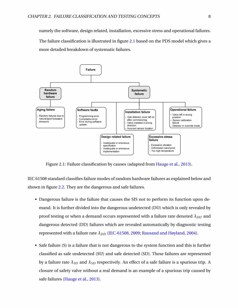
namely the software, design related, installation, excessive stress and operational failures.
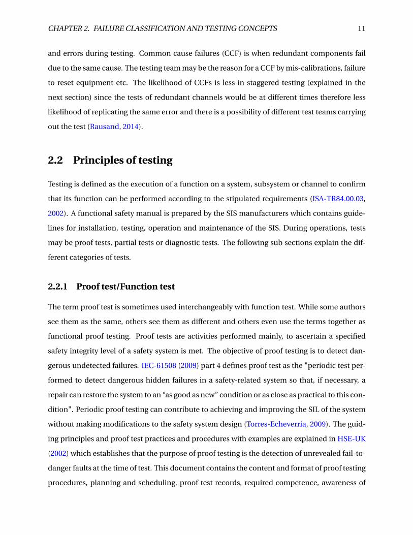
The failure classification is illustrated in figure 2.1 based on the PDS model which gives a
more detailed breakdown of systematic failures.
Figure 2.1: Failure classification by causes (adapted from Hauge et al., 2013).
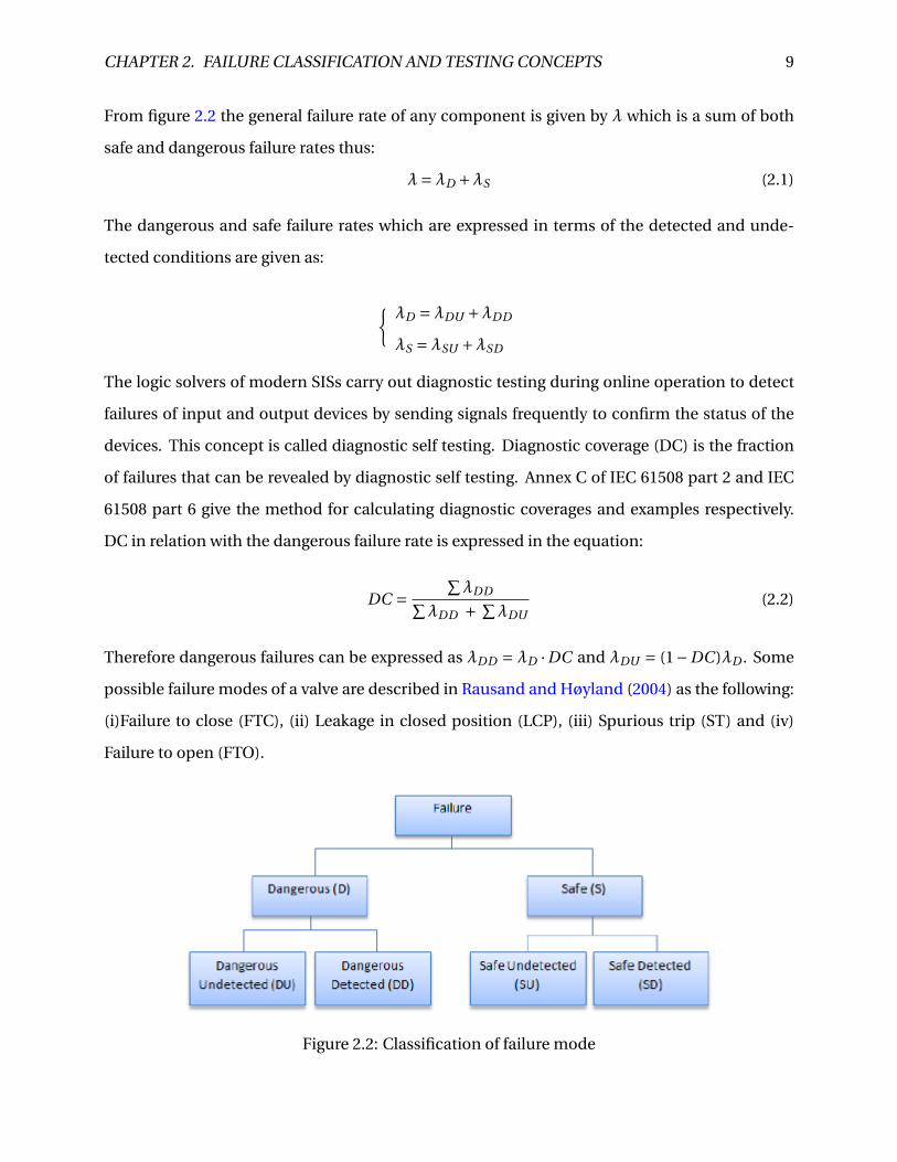
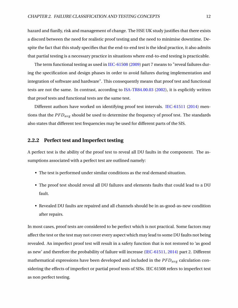
IEC 61508 standard classifies failure modes of random hardware failures as explained below and
shown in figure 2.2. They are the dangerous and safe failures.
• Dangerous failure is the failure that causes the SIS not to perform its function upon de-
mand. It is further divided into the dangerous undetected (DU) which is only revealed by
proof testing or when a demand occurs represented with a failure rate denoted λDU and
dangerous detected (DD) failures which are revealed automatically by diagnostic testing
represented with a failure rate λDD (IEC-61508, 2009; Rausand and Høyland, 2004).
• Safe failure (S) is a failure that is not dangerous to the system function and this is further
classified as safe undetected (SU) and safe detected (SD). These failures are represented
by a failure rate λSU and λSD respectively. An effect of a safe failure is a spurious trip. A
closure of safety valve without a real demand is an example of a spurious trip caused by
safe failures (Hauge et al., 2013).
CHAPTER 2. FAILURE CLASSIFICATION AND TESTING CONCEPTS 9
From figure 2.2 the general failure rate of any component is given by λ which is a sum of both
safe and dangerous failure rates thus:
λ=λD +λS (2.1)
The dangerous and safe failure rates which are expressed in terms of the detected and unde-
tected conditions are given as:
{λD =λDU +λDD
λS =λSU +λSD
The logic solvers of modern SISs carry out diagnostic testing during online operation to detect
failures of input and output devices by sending signals frequently to confirm the status of the
devices. This concept is called diagnostic self testing. Diagnostic coverage (DC) is the fraction
of failures that can be revealed by diagnostic self testing. Annex C of IEC 61508 part 2 and IEC
61508 part 6 give the method for calculating diagnostic coverages and examples respectively.
DC in relation with the dangerous failure rate is expressed in the equation:
DC =∑λDD∑
λDD + ∑λDU
(2.2)
Therefore dangerous failures can be expressed as λDD = λD ·DC and λDU = (1−DC )λD . Some
possible failure modes of a valve are described in Rausand and Høyland (2004) as the following:
(i)Failure to close (FTC), (ii) Leakage in closed position (LCP), (iii) Spurious trip (ST) and (iv)
Failure to open (FTO).
Figure 2.2: Classification of failure mode
CHAPTER 2. FAILURE CLASSIFICATION AND TESTING CONCEPTS 10
2.1.1 Common Cause Failures (CCF)
CCF is defined in IEC-61508 (2009) as failure which occurs as a result of one or more events,
causing concurrent failures of two or more separate channels in a multiple channel system
therefore leading to system failure. This could be as a result of shock or stress (e.g. tempera-
ture, humidity, vibrations) over a certain period of time. For this reason, failure of a component
can further be classified into failures due to independent causes and failures due to common
causes.
λ=λ(I ) +λ(C ) (2.3)
Independent failures are failures that affect a certain component independent of the others
whereas CCF is a concurrent failure that affects more than one component in parallel. The beta
factor model is a commonly used approach to model CCF. The (β) factor is used to partition the
total failure rate into failures due to independent and CCF.
β= λ(C )
λ(2.4)
Therefore the independent and common-cause failure rates can be expressed in terms of the
total channel failure rate λ and the common cause factor β as:
λ(I ) = (1−β)λ and λ(C ) =β ·λ
For this project, the expressions below are going to be used to differentiate the dangerous de-
tected and undetected failure rates and classify with respect to independent and CCFs respec-
tively:
λ(i )DU = (1−β)λDU and λ(c)
DU =β ·λDU
λ(i )DD = (1−βD )λDD and λ(c)
DD =βD ·λDD
2.1.2 Influence of Common Cause Failures on testing
Redundancy enhances the performance of SISs but the reliability effect may be reduced if the
components are exposed to factors like design errors, operational errors, maintenance errors
CHAPTER 2. FAILURE CLASSIFICATION AND TESTING CONCEPTS 11
and errors during testing. Common cause failures (CCF) is when redundant components fail
due to the same cause. The testing team may be the reason for a CCF by mis-calibrations, failure
to reset equipment etc. The likelihood of CCFs is less in staggered testing (explained in the
next section) since the tests of redundant channels would be at different times therefore less
likelihood of replicating the same error and there is a possibility of different test teams carrying
out the test (Rausand, 2014).
2.2 Principles of testing
Testing is defined as the execution of a function on a system, subsystem or channel to confirm
that its function can be performed according to the stipulated requirements (ISA-TR84.00.03,
2002). A functional safety manual is prepared by the SIS manufacturers which contains guide-
lines for installation, testing, operation and maintenance of the SIS. During operations, tests
may be proof tests, partial tests or diagnostic tests. The following sub sections explain the dif-
ferent categories of tests.
2.2.1 Proof test/Function test
The term proof test is sometimes used interchangeably with function test. While some authors
see them as the same, others see them as different and others even use the terms together as
functional proof testing. Proof tests are activities performed mainly, to ascertain a specified
safety integrity level of a safety system is met. The objective of proof testing is to detect dan-
gerous undetected failures. IEC-61508 (2009) part 4 defines proof test as the "periodic test per-
formed to detect dangerous hidden failures in a safety-related system so that, if necessary, a
repair can restore the system to an “as good as new” condition or as close as practical to this con-
dition". Periodic proof testing can contribute to achieving and improving the SIL of the system
without making modifications to the safety system design (Torres-Echeverria, 2009). The guid-
ing principles and proof test practices and procedures with examples are explained in HSE-UK
(2002) which establishes that the purpose of proof testing is the detection of unrevealed fail-to-
danger faults at the time of test. This document contains the content and format of proof testing
procedures, planning and scheduling, proof test records, required competence, awareness of
CHAPTER 2. FAILURE CLASSIFICATION AND TESTING CONCEPTS 12
hazard and fianlly, risk and management of change. The HSE UK study justifies that there exists
a discord between the need for realistic proof testing and the need to minimise downtime. De-
spite the fact that this study specifies that the end-to-end test is the ideal practice, it also admits
that partial testing is a necessary practice in situations where end-to-end testing is practicable.
The term functional testing as used in IEC-61508 (2009) part 7 means to "reveal failures dur-
ing the specification and design phases in order to avoid failures during implementation and
integration of software and hardware". This consequently means that proof test and functional
tests are not the same. In contrast, according to ISA-TR84.00.03 (2002), it is explicitly written
that proof tests and functional tests are the same test.
Different authors have worked on identifying proof test intervals. IEC-61511 (2014) men-
tions that the PF Dav g should be used to determine the frequency of proof test. The standards
also states that different test frequencies may be used for different parts of the SIS.
2.2.2 Perfect test and Imperfect testing
A perfect test is the ability of the proof test to reveal all DU faults in the component. The as-
sumptions associated with a perfect test are outlined namely:
• The test is performed under similar conditions as the real demand situation.
• The proof test should reveal all DU failures and elements faults that could lead to a DU
fault.
• Revealed DU faults are repaired and all channels should be in as-good-as-new condition
after repairs.
In most cases, proof tests are considered to be perfect which is not practical. Some factors may
affect the test or the test may not cover every aspect which may lead to some DU faults not being
revealed. An imperfect proof test will result in a safety function that is not restored to ‘as good
as new’ and therefore the probability of failure will increase (IEC-61511, 2014) part 2. Different
mathematical expressions have been developed and included in the PF Dav g calculation con-
sidering the effects of imperfect or partial proof tests of SISs. IEC 61508 refers to imperfect test
as non perfect testing.
CHAPTER 2. FAILURE CLASSIFICATION AND TESTING CONCEPTS 13
Bukowski and Van Beurden (2009) classified imperfect testing under two categories: Incom-
plete and incorrect testing.
• Proof test completeness is here defined as the probability that all dangerous failures are
revealed/checked for during a proof test which is a function of the component and the
tests that are executed. Based on this definition, the completeness/incompleteness of
proof tests can be part of partial or full proof tests. Incomplete proof test therefore has to
do with the limitation of the test.
• Proof test correctness indicates the probability that the actual test is correctly executed
by the test team as specified and that all existing faults are revealed, repaired and no new
problems are introduced during the test. This is therefore seen as a function of the main-
tenance capabilities and culture at a specific plant site. Incorrect proof test has to do with
the limitations of those performing the test.
Impact analyses shows that test completeness has a higher impact on PFD than test correctness
(Brissaud et al., 2012; Bukowski and Van Beurden, 2009).
2.2.3 Reasons for having imperfect test
The subsection above mentioned imperfectness of tests and this may be a situation whereby test
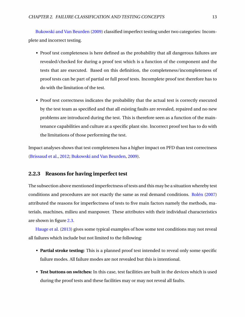
conditions and procedures are not exactly the same as real demand conditions. Rolén (2007)
attributed the reasons for imperfectness of tests to five main factors namely the methods, ma-
terials, machines, milieu and manpower. These attributes with their individual characteristics
are shown in figure 2.3.
Hauge et al. (2013) gives some typical examples of how some test conditions may not reveal
all failures which include but not limited to the following:
• Partial stroke testing: This is a planned proof test intended to reveal only some specific
failure modes. All failure modes are not revealed but this is intentional.
• Test buttons on switches: In this case, test facilities are built in the devices which is used
during the proof tests and these facilities may or may not reveal all faults.
CHAPTER 2. FAILURE CLASSIFICATION AND TESTING CONCEPTS 14
Figure 2.3: Fishbone diagram for causes of imperfect testing (adapted from Rolén, 2007).
• Transmitters put into test mode and signals injected: The test mode may have bypassed
the original functioning mode of the transmitters and the injection of signals with smart/fieldbus
transmitters may be different from real situation hence not revealing all failure modes.
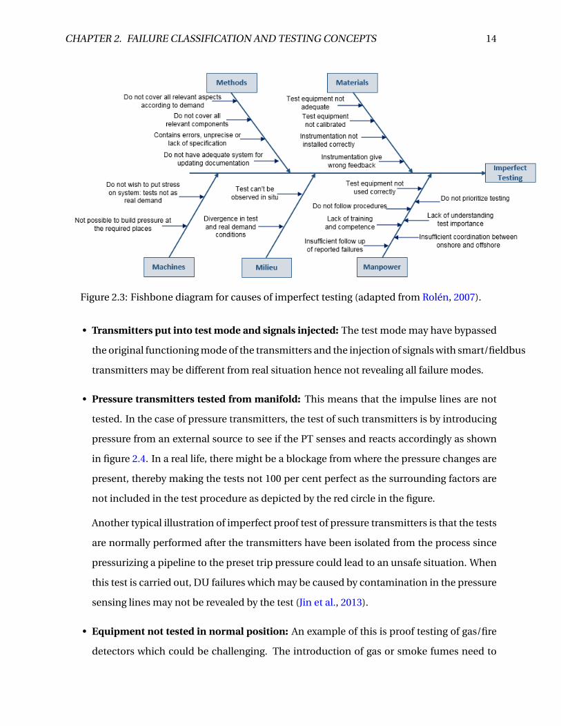
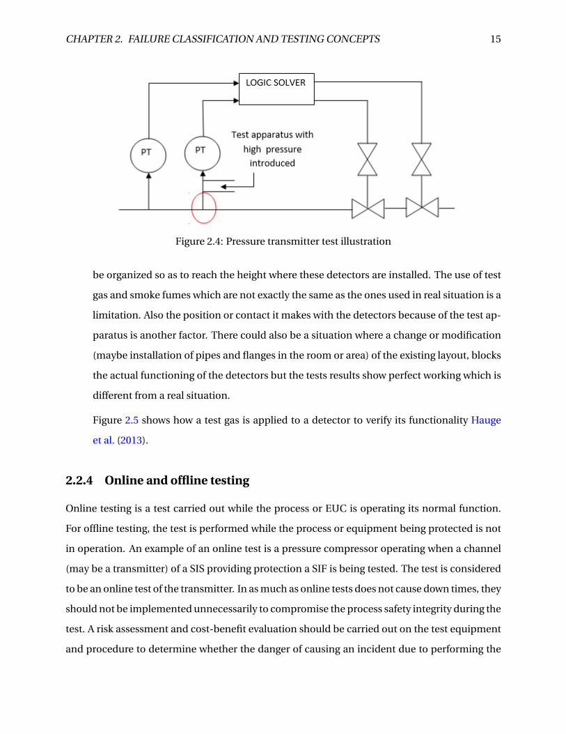
• Pressure transmitters tested from manifold: This means that the impulse lines are not
tested. In the case of pressure transmitters, the test of such transmitters is by introducing
pressure from an external source to see if the PT senses and reacts accordingly as shown
in figure 2.4. In a real life, there might be a blockage from where the pressure changes are
present, thereby making the tests not 100 per cent perfect as the surrounding factors are
not included in the test procedure as depicted by the red circle in the figure.
Another typical illustration of imperfect proof test of pressure transmitters is that the tests
are normally performed after the transmitters have been isolated from the process since
pressurizing a pipeline to the preset trip pressure could lead to an unsafe situation. When
this test is carried out, DU failures which may be caused by contamination in the pressure
sensing lines may not be revealed by the test (Jin et al., 2013).
• Equipment not tested in normal position: An example of this is proof testing of gas/fire
detectors which could be challenging. The introduction of gas or smoke fumes need to
CHAPTER 2. FAILURE CLASSIFICATION AND TESTING CONCEPTS 15
Figure 2.4: Pressure transmitter test illustration
be organized so as to reach the height where these detectors are installed. The use of test
gas and smoke fumes which are not exactly the same as the ones used in real situation is a
limitation. Also the position or contact it makes with the detectors because of the test ap-
paratus is another factor. There could also be a situation where a change or modification
(maybe installation of pipes and flanges in the room or area) of the existing layout, blocks
the actual functioning of the detectors but the tests results show perfect working which is
different from a real situation.
Figure 2.5 shows how a test gas is applied to a detector to verify its functionality Hauge
et al. (2013).
2.2.4 Online and offline testing
Online testing is a test carried out while the process or EUC is operating its normal function.
For offline testing, the test is performed while the process or equipment being protected is not
in operation. An example of an online test is a pressure compressor operating when a channel
(may be a transmitter) of a SIS providing protection a SIF is being tested. The test is considered
to be an online test of the transmitter. In as much as online tests does not cause down times, they
should not be implemented unnecessarily to compromise the process safety integrity during the
test. A risk assessment and cost-benefit evaluation should be carried out on the test equipment
and procedure to determine whether the danger of causing an incident due to performing the

CHAPTER 2. FAILURE CLASSIFICATION AND TESTING CONCEPTS 16
Figure 2.5: Test apparatus for gas detectors
on-line test is greater than the danger of not discovering the failure (ISA-TR84.00.03, 2002).
2.2.5 Full proof test and partial test
Full proof test is a test performed at intervals meant to reveal all latent failures of the equipment
or component being tested. Proof testing in most cases requires a system shutdown which af-
fects the production and leads to production downtime. A partial proof test is a planned test is
implemented to enable extension of the full proof test in order to avoid production loss while
still maintaining the integrity of the system. A partial proof test is designed to test one or more
specific failure modes of a channel without significantly disturbing the EUC. The HSE-UK (2002)
classifies partial testing under two categories namely:
• Testing of system components at different times and frequencies which is called staggered
testing.
CHAPTER 2. FAILURE CLASSIFICATION AND TESTING CONCEPTS 17
• Testing of the subsets of functions of single components in the form of measurement sim-
ulation or the partial stroking of valves.
2.3 Partial Stroke Testing
Partial stroking of safety valves is a type of partial test to detect failure mode like "failure to close
on demand" but it is not possible to detect a failure mode like "leakage in closed position" (Jin
and Rausand, 2014). Though partial tests are not as effective as full tests, they have some advan-
tages over full tests. They are less costly and less time consuming and also some safety devices
are preferably partially tested in order not to cause degradation or destruction (Brissaud et al.,
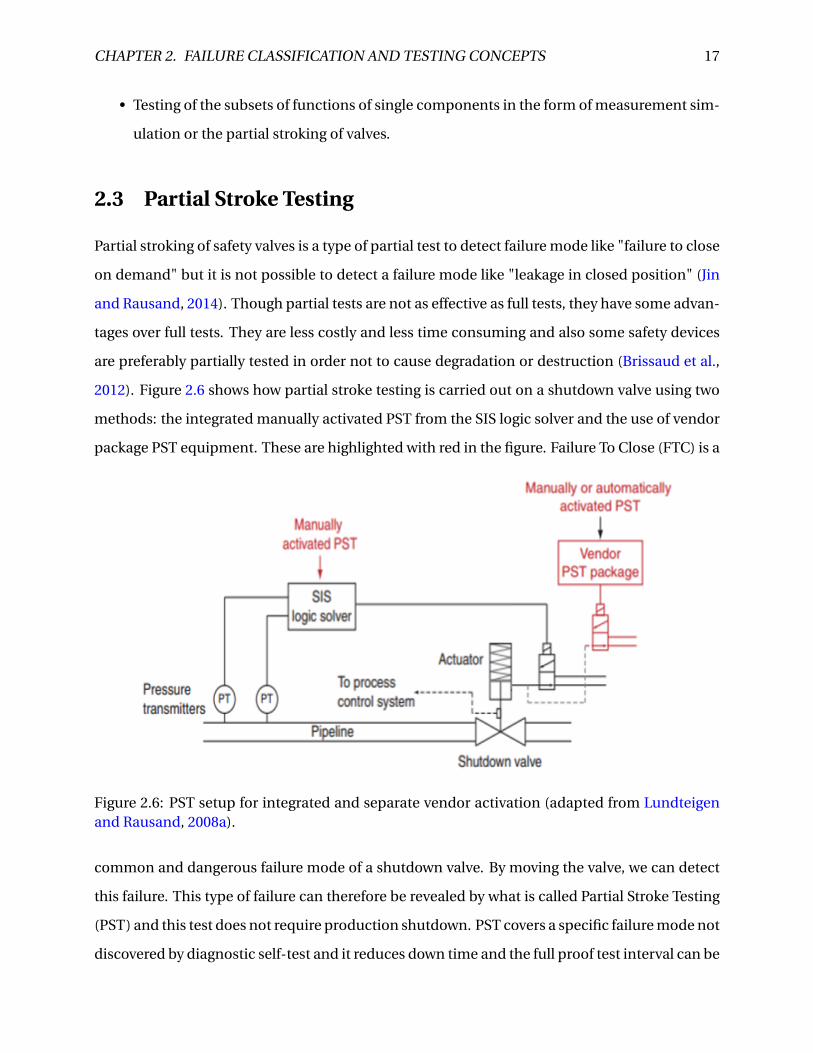
2012). Figure 2.6 shows how partial stroke testing is carried out on a shutdown valve using two
methods: the integrated manually activated PST from the SIS logic solver and the use of vendor
package PST equipment. These are highlighted with red in the figure. Failure To Close (FTC) is a
Figure 2.6: PST setup for integrated and separate vendor activation (adapted from Lundteigenand Rausand, 2008a).
common and dangerous failure mode of a shutdown valve. By moving the valve, we can detect
this failure. This type of failure can therefore be revealed by what is called Partial Stroke Testing
(PST) and this test does not require production shutdown. PST covers a specific failure mode not
discovered by diagnostic self-test and it reduces down time and the full proof test interval can be
CHAPTER 2. FAILURE CLASSIFICATION AND TESTING CONCEPTS 18
made longer. Full stroke operation and leakage testing requires a shutdown of process. Partial
stroke testing has been introduced to supplement functional testing (Ali et al., 2004; Summers
and Zachary, 2000). PST is a way by which a valve is partially opened or closed then returned to
its initial position to detect several specific types of DU failures without interrupting the process.
The total PFD where a partial test is implemented is given by the equation:
PF Dav g = PF DF T +PF DPT
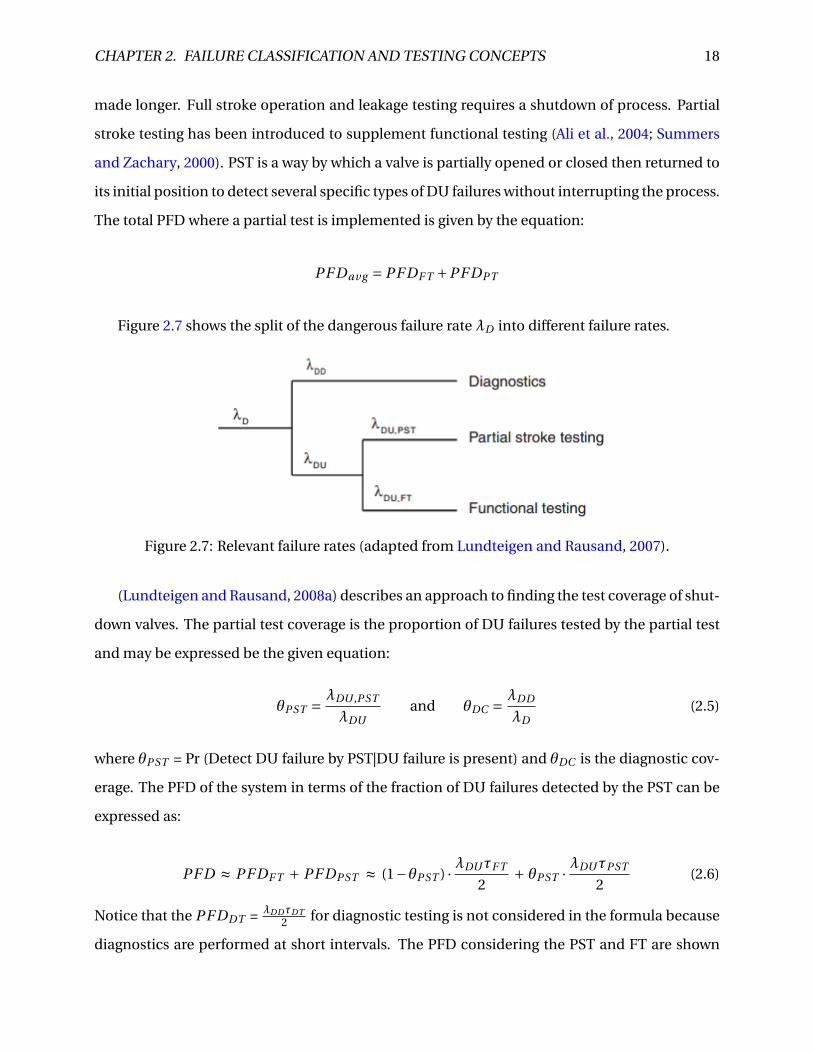
Figure 2.7 shows the split of the dangerous failure rate λD into different failure rates.
Figure 2.7: Relevant failure rates (adapted from Lundteigen and Rausand, 2007).
(Lundteigen and Rausand, 2008a) describes an approach to finding the test coverage of shut-
down valves. The partial test coverage is the proportion of DU failures tested by the partial test
and may be expressed be the given equation:
θPST = λDU ,PST
λDUand θDC = λDD
λD(2.5)
where θPST = Pr (Detect DU failure by PST|DU failure is present) and θDC is the diagnostic cov-
erage. The PFD of the system in terms of the fraction of DU failures detected by the PST can be
expressed as:
PF D ≈ PF DF T + PF DPST ≈ (1−θPST ) · λDUτF T
2+ θPST · λDUτPST
2(2.6)
Notice that the PF DDT = λDDτDT2 for diagnostic testing is not considered in the formula because
diagnostics are performed at short intervals. The PFD considering the PST and FT are shown
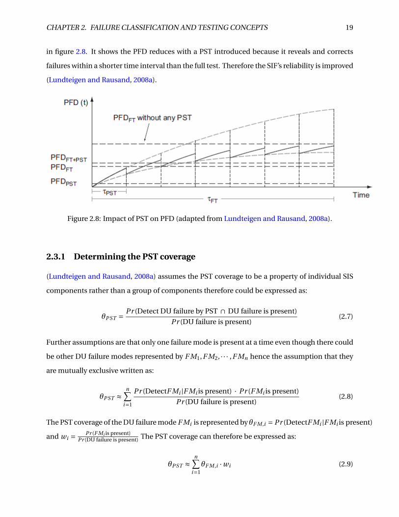
CHAPTER 2. FAILURE CLASSIFICATION AND TESTING CONCEPTS 19
in figure 2.8. It shows the PFD reduces with a PST introduced because it reveals and corrects
failures within a shorter time interval than the full test. Therefore the SIF’s reliability is improved
(Lundteigen and Rausand, 2008a).
Figure 2.8: Impact of PST on PFD (adapted from Lundteigen and Rausand, 2008a).
2.3.1 Determining the PST coverage
(Lundteigen and Rausand, 2008a) assumes the PST coverage to be a property of individual SIS
components rather than a group of components therefore could be expressed as:
θPST = Pr (Detect DU failure by PST ∩ DU failure is present)
Pr (DU failure is present)(2.7)
Further assumptions are that only one failure mode is present at a time even though there could
be other DU failure modes represented by F M1,F M2, · · · ,F Mn hence the assumption that they
are mutually exclusive written as:
θPST ≈n∑
i=1
Pr (DetectF Mi |F Mi is present) · Pr (F Mi is present)
Pr (DU failure is present)(2.8)
The PST coverage of the DU failure mode F Mi is represented by θF M ,i = Pr (DetectF Mi |F Mi is present)
and wi = Pr (F Mi is present)Pr (DU failure is present) The PST coverage can therefore be expressed as:
θPST ≈n∑
i=1θF M ,i ·wi (2.9)
CHAPTER 2. FAILURE CLASSIFICATION AND TESTING CONCEPTS 20
This method suggests that θF M ,i can be determined by evaluating the failure mode’s revealability
and reliability of the test which can be achieved by expert judgement and checklists respectively.
Details of how the PST coverage is determined is explained in 6 steps
• Step 1: Becoming familiar with the PST and its implementation.
This includes getting acquainted with the SIS components operated during a PST, the
functional safety requirements of the SIS components like valve closing time, PST initi-
ation and control by dedicated hardware and software, process control system and finally
the operational and environmental conditions under which the SIF operates, including
fluid characteristics, temperature and pressure.
• Step 2: Analyze the PST hardware and software.
The FMEA analysis is suggested to identify and analyze potential PST hardware and soft-
ware failures and the effect these failures may have on the PST execution and the SIS. This
should be done in collaboration with end users and vendors and it serves as a basis for the
checklist.
• Step 3: Determine the PST reliability.
Checklist containing questions which gives credits to the system behavior is used to pro-
vide reliable and useful test results. Each question is weighted according to importance.
for details of this step refer to Lundteigen and Rausand (2008a).
• Step 4: Determine the revealability (per failure mode).
Deciding whether or not the failure mode may be revealed by the PST. A failure mode may
also only be revealed for a portion of the failures in each failure mode. A failure mode that
is fully observable is given the revealability factor 100 percent and when not observable
at all 0 percent. A failure mode may also be revealable with a certain probability, which is
used as the revealability factor.
• Step 5: Determine the failure mode weight.
The weight of failure mode is the fraction the specific failure mode among all failures,
shown previously with the equation for wi . The failure mode weight is determined by
expert judgment or by analysis of historical data.
CHAPTER 2. FAILURE CLASSIFICATION AND TESTING CONCEPTS 21
• Step 6: Determine the PST coverage.
The PST coverage θPST can now be calculated using the formula 5.5 since the values needed
have been derived from previous steps.
2.4 Relationship between the types of tests
Though the term proof tests and functional tests may be mixed up or used interchangeably, it is
clear from the above sections that they are different. Function test is a test procedure of running
or activating a function of the SIF. This does not include other tests like pressure tests (calibra-
tion) and leakage tests of valves. Therefore proof tests encompasses both functional tests and
leakage tests with other kinds of tests and calibrations. OLF-070 (2004) uses the term functional
proof testing to mean the same thing. The guideline’s requirement of proof tests is to verify
that the entire SIS loop including the sensors, logic solvers and the final elements are work-
ing adequately. OLF 070 specifies the aspects which the proof test should cover summarized in
complete system functionality. A full proof test and partial proof test may be imperfect if they
don’t reveal the faults they are designed and expected to reveal.
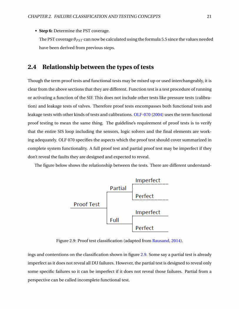
The figure below shows the relationship between the tests. There are different understand-
Figure 2.9: Proof test classification (adapted from Rausand, 2014).
ings and contentions on the classification shown in figure 2.9. Some say a partial test is already
imperfect as it does not reveal all DU failures. However, the partial test is designed to reveal only
some specific failures so it can be imperfect if it does not reveal those failures. Partial from a
perspective can be called incomplete functional test.
CHAPTER 2. FAILURE CLASSIFICATION AND TESTING CONCEPTS 22
2.5 Adverse effects of full proof testing and partial testing
In as much as proof test ensures that a safety system is able to function as required upon de-
mand, it also presents some challenges and adverse effects. One of these effects is the down
time of the safety system due to full proof tests. Human error is another factor. Lundteigen and
Rausand (2008b) mentioned that human error during tests is an additional factor contributing
to increase in spurious activations of a SIS. In the differences between diagnostics and func-
tional testing, human interaction during test preparation, execution and restoration has an ef-
fect which could be adverse (Lundteigen and Rausand, 2008a). The concepts of human error
which could be failure to detect a fault and leaving the component in bad state after test was
used in the analysis of optimal test interval. Operator error and the probability of test-caused
failure were modelled as constant unavailability and added to the time-dependent unavailabil-
ity quantification (Lee et al., 1990).
Partial tests on the other hand has its disadvantages. From the definition, only a portion of
DU failures are revealed which leaves other dangerous undetected failures which could prevent
the system from responding in case of a demand. Secondly, the frequent operation leads to wear
and degradation of the system. In case of a valve, there is a potential increase in spurious trip
rate since the valve may continue to fail safe position instead of returning to the initial position.
2.6 Test strategies
Test strategies are classified as simultaneous, sequential, staggered and independent tests ac-
cording to Torres-Echeverria et al. (2009). Proof testing strategies specify the scheduling of proof
tests of redundant components with respect to one another. The different strategies are ex-
plained the the subsections. A petri net model for the different testing strategies using a 1oo2
subsytem is shown (Liu and Rausand, 2013).
• Simultaneous testing : This is when a number N of redundant components are tested at
the same time where the time of proof test t is the same for all components. This means
that the same number of crews as the components are available during the test. In situ-
ation where the safety system must always be in a functioning state, this strategy is not
CHAPTER 2. FAILURE CLASSIFICATION AND TESTING CONCEPTS 23
suitable because the safety system is made unavailable during the test period.
• Sequential testing : Sequential testing is a situation where N redundant components are
tested one after the other. A second component test can only begin when the first com-
ponent has been tested and restored to a working state. This sequence repeats for all
the components of the subsystem. This strategy enables the SIS to operate in a degraded
mode since n −1 channels are available when a channel is being tested. (Cepin, 1995; Liu
and Rausand, 2013).
• Staggered testing : This is a type of sequential testing where the n tests are spread out over
the entire test interval. This strategy increases the safety availability of the SIS. IEC 61508
part 6 mentions that If the tests are staggered and adequate procedures implemented,
the likelihood of detecting CCFs increases and it is an effective method of reducing the
CCF for systems operating in a low demand mode of operation. staggered testing has its
adverse effects. The recurrent tests requires extra maintenance management and the cost
of testing could increase significantly. An example is a situation where the equipment to
be tested is offshore. Hiring the test vessels for different test times means extra cost.
• Independent testing : In the case of independent testing, the time of test of the N compo-
nents are in a random order. There is no specific test schedule between the components
(Torres-Echeverria et al., 2009).
Chapter 3
Analytical formulas for performance of SIS
3.1 Analytical approach based on full proof tests
Analytical formulas are used to determine the probability of failure of a SIS. These formulations
are only approximations. Different analytical formulas found in the literature for PFD average
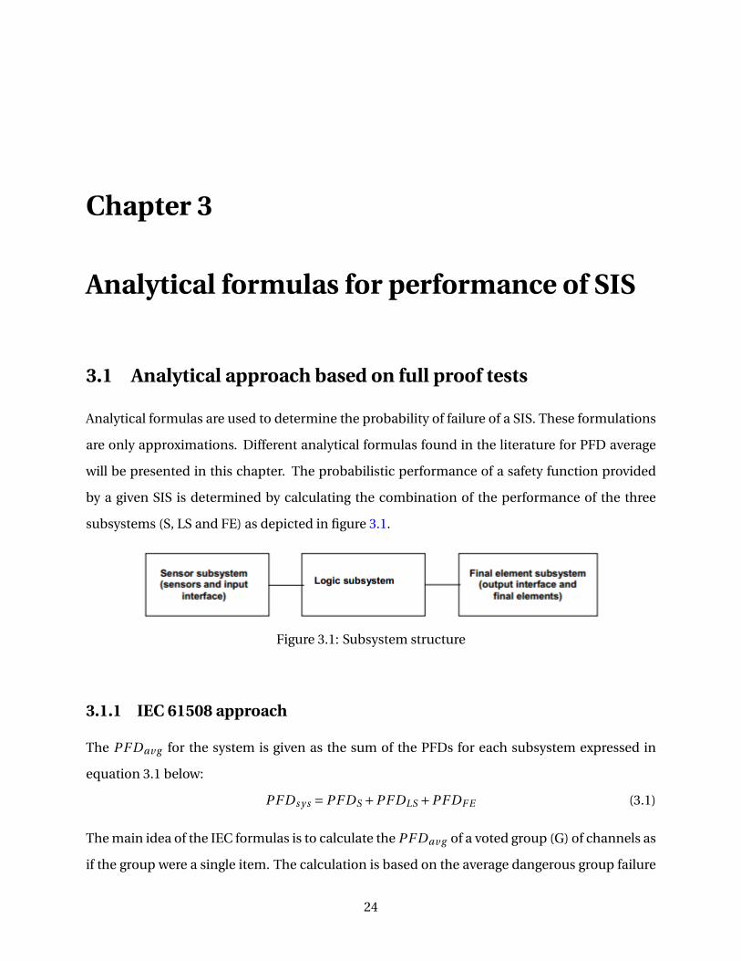
will be presented in this chapter. The probabilistic performance of a safety function provided
by a given SIS is determined by calculating the combination of the performance of the three
subsystems (S, LS and FE) as depicted in figure 3.1.
Figure 3.1: Subsystem structure
3.1.1 IEC 61508 approach
The PF Dav g for the system is given as the sum of the PFDs for each subsystem expressed in
equation 3.1 below:
PF Ds y s = PF DS +PF DLS +PF DF E (3.1)
The main idea of the IEC formulas is to calculate the PF Dav g of a voted group (G) of channels as
if the group were a single item. The calculation is based on the average dangerous group failure
24
CHAPTER 3. ANALYTICAL FORMULAS FOR PERFORMANCE OF SIS 25
frequency (λD,G ) and the group-equivalent mean downtime (tGE ). The PF Dav g for the group is
calculated as:
PF D (G)av g =λD,G · tGE (3.2)
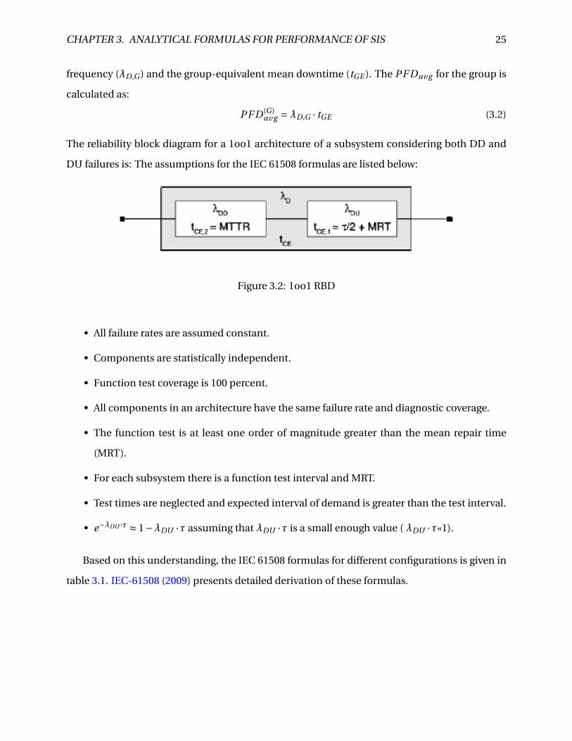
The reliability block diagram for a 1oo1 architecture of a subsystem considering both DD and
DU failures is: The assumptions for the IEC 61508 formulas are listed below:
Figure 3.2: 1oo1 RBD
• All failure rates are assumed constant.
• Components are statistically independent.
• Function test coverage is 100 percent.
• All components in an architecture have the same failure rate and diagnostic coverage.
• The function test is at least one order of magnitude greater than the mean repair time
(MRT).
• For each subsystem there is a function test interval and MRT.
• Test times are neglected and expected interval of demand is greater than the test interval.
• e−λDU ·τ ≈ 1−λDU ·τ assuming that λDU ·τ is a small enough value ( λDU ·τ«1).
Based on this understanding, the IEC 61508 formulas for different configurations is given in
table 3.1. IEC-61508 (2009) presents detailed derivation of these formulas.
CHAPTER 3. ANALYTICAL FORMULAS FOR PERFORMANCE OF SIS 26
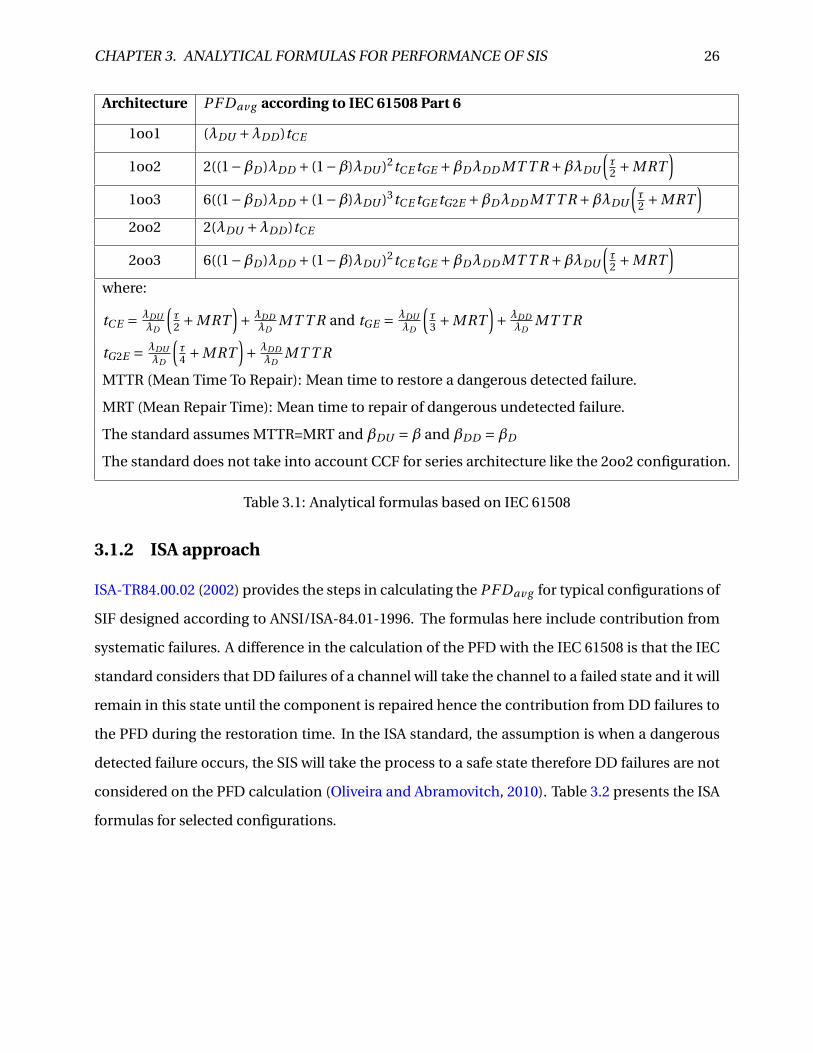
Architecture PF Dav g according to IEC 61508 Part 6
1oo1 (λDU +λDD )tC E
1oo2 2((1−βD )λDD + (1−β)λDU )2tC E tGE +βDλDD MT T R +βλDU
(τ2 +MRT
)1oo3 6((1−βD )λDD + (1−β)λDU )3tC E tGE tG2E +βDλDD MT T R +βλDU
(τ2 +MRT
)2oo2 2(λDU +λDD )tC E
2oo3 6((1−βD )λDD + (1−β)λDU )2tC E tGE +βDλDD MT T R +βλDU
(τ2 +MRT
)where:
tC E = λDUλD
(τ2 +MRT
)+ λDD
λDMT T R and tGE = λDU
λD
(τ3 +MRT
)+ λDD
λDMT T R
tG2E = λDUλD
(τ4 +MRT
)+ λDD
λDMT T R
MTTR (Mean Time To Repair): Mean time to restore a dangerous detected failure.
MRT (Mean Repair Time): Mean time to repair of dangerous undetected failure.
The standard assumes MTTR=MRT and βDU =β and βDD =βD
The standard does not take into account CCF for series architecture like the 2oo2 configuration.
Table 3.1: Analytical formulas based on IEC 61508
3.1.2 ISA approach
ISA-TR84.00.02 (2002) provides the steps in calculating the PF Dav g for typical configurations of
SIF designed according to ANSI/ISA-84.01-1996. The formulas here include contribution from
systematic failures. A difference in the calculation of the PFD with the IEC 61508 is that the IEC
standard considers that DD failures of a channel will take the channel to a failed state and it will
remain in this state until the component is repaired hence the contribution from DD failures to
the PFD during the restoration time. In the ISA standard, the assumption is when a dangerous
detected failure occurs, the SIS will take the process to a safe state therefore DD failures are not
considered on the PFD calculation (Oliveira and Abramovitch, 2010). Table 3.2 presents the ISA
formulas for selected configurations.
CHAPTER 3. ANALYTICAL FORMULAS FOR PERFORMANCE OF SIS 27
Architecture PF Dav g according to ISA-TR84.00.02-2002
1oo1(λDU · τ2
)+
(λD
F · τ2)≈λDU · τ2
1oo2
(λ2
DU · τ2
3
)+
(λDU ·λDD ·MT T R ·τ
)+βλDU · τ2
1oo3
(λ3
DU · τ3
4
)+
(λ2
DU ·λDD ·MT T R ·τ2)+βλDU · τ2
2oo2(λDU ·τ
)+
(βλDU ·τ
)2oo3
(λ2
DU ·τ2)+
(3 ·λDU ·λDD ·MT T R ·τ
)+βλDU · τ2
where:
λDF is the dangerous systematic failure rate.
τ is the time interval between manual functional tests of the component.
Table 3.2: Analytical formulas based on ISA-TR84.00.02-2002
3.1.3 The PDS method
SINTEF developed the PDS method based on the IEC 61508 and 61511 principles and it is widely
used in the Norwegian petroleum industry. The main differences of this method and the IEC
standards in relation to the calculation of PFD is a different CCF model called the multiple beta-
factor model. The PDS Beta factor model distinguishes between different types of voting. The
configuration is considered in relation to the rate of CCFs and the beta-factor of an MooN voting
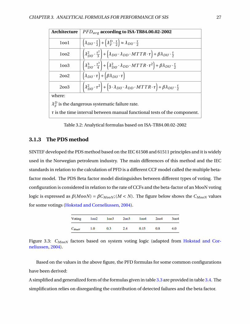
logic is expressed as β(MooN ) = βCMooN ; (M < N ). The figure below shows the CMooN values
for some votings (Hokstad and Corneliussen, 2004).
Figure 3.3: CMooN factors based on system voting logic (adapted from Hokstad and Cor-neliussen, 2004).
Based on the values in the above figure, the PFD formulas for some common configurations
have been derived:
A simplified and generalized form of the formulas given in table 3.3 are provided in table 3.4. The
simplification relies on disregarding the contribution of detected failures and the beta factor.
CHAPTER 3. ANALYTICAL FORMULAS FOR PERFORMANCE OF SIS 28
Architecture PF Dav g according to PDS method
1oo1 λDU · τ2 +λDD ·MT T R
1oo2 (1−β)2λ2DU · τ2
3 +2(1−β)λDD ·λDU ·MT T R · τ2 +β(λDD ·MT T R +λDU · τ2
)1oo3 0.3
[β ·λDD ·MT T R +βλDU · τ2
]+ 1
4
[(1−1.7β)λDU ·τ
]3+3(1−1.7β)λDD ·MT T R ·βλDU · τ2
2oo2 (2−β)(λDU · τ2
)+β ·λDD ·MT T R
2oo3 2.4 ·βλDU · τ2 +[
(1−1.7β)λDU ·τ]2
+3(1−1.7β)λDD ·MT T R ·βλDU · τ2SINTEF does not use the normal β factor model for CCF.
The coefficient β for CCF is the same for both detected and undetected βDU =βDD =β.
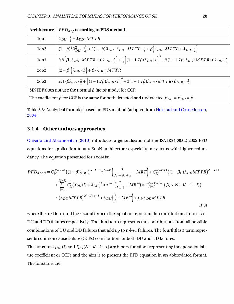
Table 3.3: Analytical formulas based on PDS method (adapted from Hokstad and Corneliussen,2004)
3.1.4 Other authors approaches
Oliveira and Abramovitch (2010) introduces a generalization of the ISATR84.00.02-2002 PFD
equations for application to any KooN architecture especially to systems with higher redun-
dancy. The equation presented for KooN is:
PF DK ooN =C N−K+1N
((1−β)λDU
)N−K+1τN−K
(τ
N −K +2+MRT
)+C N−K+1
N
((1−βD )λDD MT T R
)N−K+1
+N−K∑i=1
C iN
(fDU (i )×λDU
)i ×τi−1( τ
i +1+MRT
)×C N−K+1−iN−i
(fDD (N −K +1− i )
)× (
λDD MT T R)N−K+1−i +βDU
(τ
2+MRT
)+βDλDD MT T R
(3.3)
where the first term and the second term in the equation represent the contributions from n-k+1
DU and DD failures respectively. The third term represents the contributions from all possible
combinations of DU and DD failures that add up to n-k+1 failures. The fourth(last) term repre-
sents common cause failure (CCFs) contribution for both DU and DD failures.
The functions fDU (i ) and fDD (N −K +1− i ) are binary functions representing independent fail-
ure coefficient or CCFs and the aim is to present the PFD equation in an abbreviated format.
The functions are:
CHAPTER 3. ANALYTICAL FORMULAS FOR PERFORMANCE OF SIS 29
Voting Common cause contribution Contribution from independent failures
1oo1 - λDU ·τ/2
1oo2 β ·λDU ·τ/2 +[λDU ·τ]2/3
2oo2 - 2 ·λDU ·τ/2
1oo3 C1oo3 ·β ·λDU ·τ/2 +[λDU ·τ]3/4
2oo3 C1oo3 ·β ·λDU ·τ/2 +[λDU ·τ]2
3oo3 - 3 ·λDU ·τ/2
1ooN; N=2,3,.. C1ooN ·β ·λDU ·τ/2 + 1N+1 ·
[λDU ·τ]N
MooN, M<N; N=2,3,.. CMooN ·β ·λDU ·τ/2 + N !(N−M+2)!·(M−1)! ·
[λDU ·τ]N−M+1
NooN; N=1,2,3,.. - N ·λDU ·τ/2
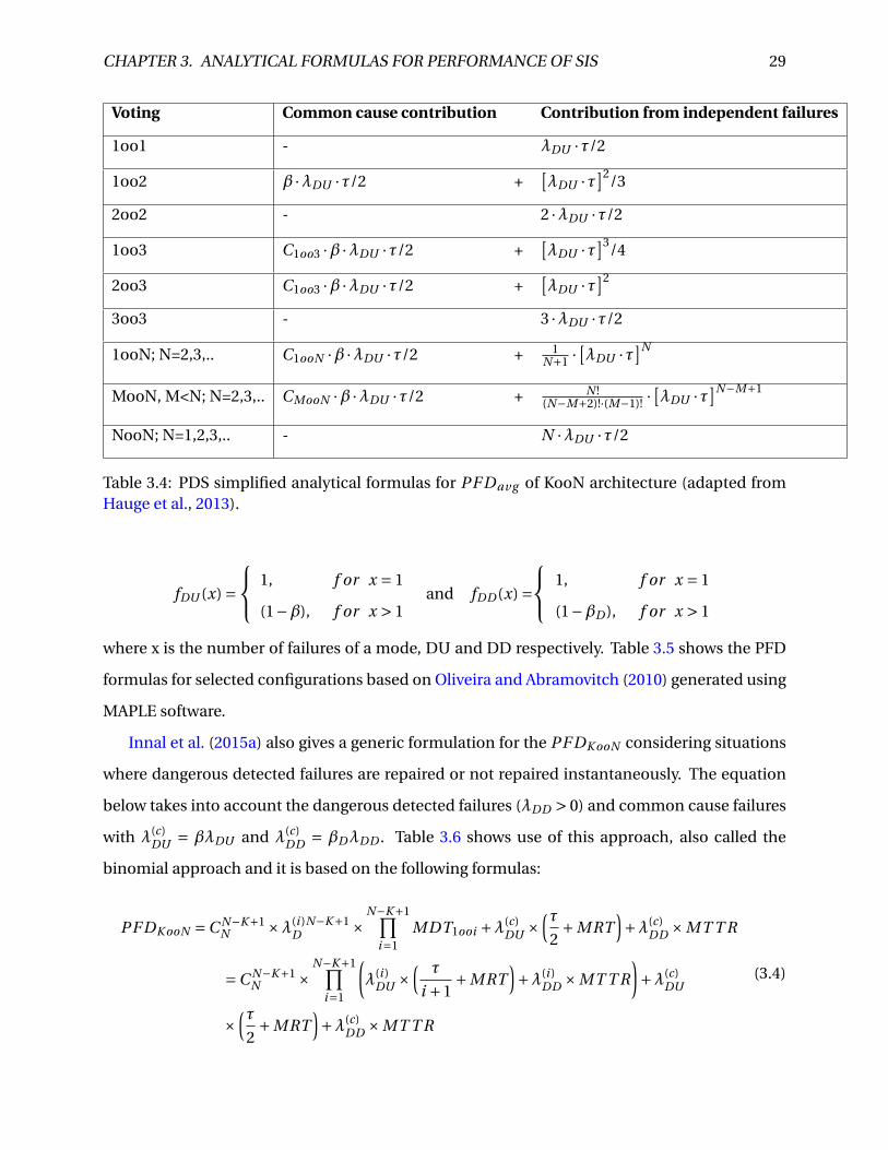
Table 3.4: PDS simplified analytical formulas for PF Dav g of KooN architecture (adapted fromHauge et al., 2013).
fDU (x) = 1, f or x = 1
(1−β), f or x > 1and fDD (x) =
1, f or x = 1
(1−βD ), f or x > 1
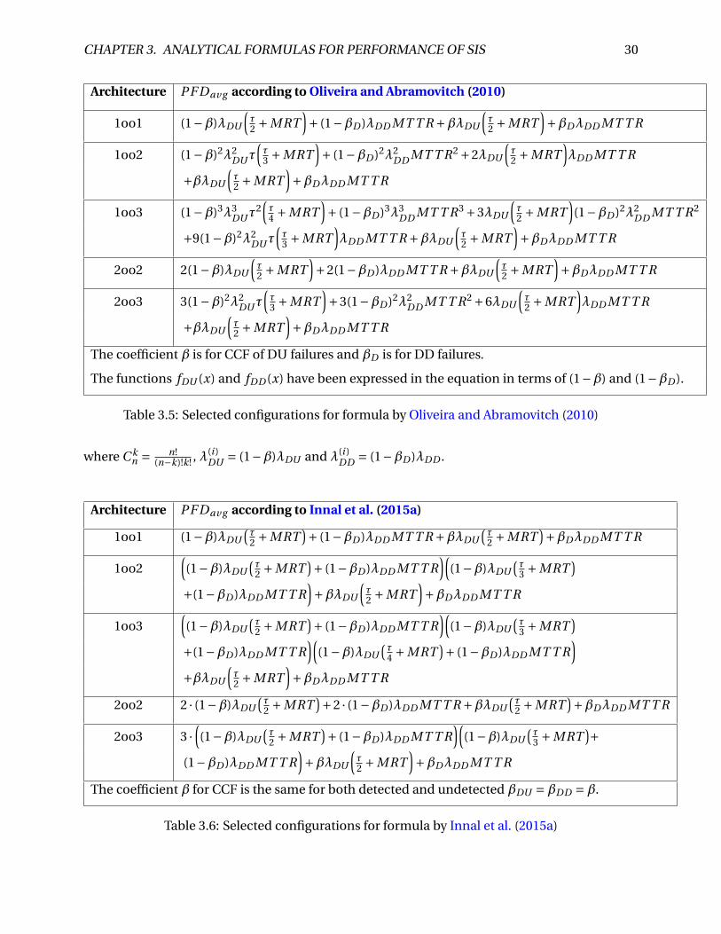
where x is the number of failures of a mode, DU and DD respectively. Table 3.5 shows the PFD
formulas for selected configurations based on Oliveira and Abramovitch (2010) generated using
MAPLE software.
Innal et al. (2015a) also gives a generic formulation for the PF DK ooN considering situations
where dangerous detected failures are repaired or not repaired instantaneously. The equation
below takes into account the dangerous detected failures (λDD > 0) and common cause failures
with λ(c)DU = βλDU and λ(c)
DD = βDλDD . Table 3.6 shows use of this approach, also called the
binomial approach and it is based on the following formulas:
PF DK ooN =C N−K+1N ×λ(i )N−K+1
D ×N−K+1∏
i=1MDT1ooi +λ(c)
DU ×(τ
2+MRT
)+λ(c)
DD ×MT T R
=C N−K+1N ×
N−K+1∏i=1
(λ(i )
DU ×( τ
i +1+MRT
)+λ(i )
DD ×MT T R
)+λ(c)
DU
×(τ
2+MRT
)+λ(c)
DD ×MT T R
(3.4)
CHAPTER 3. ANALYTICAL FORMULAS FOR PERFORMANCE OF SIS 30
Architecture PF Dav g according to Oliveira and Abramovitch (2010)
1oo1 (1−β)λDU
(τ2 +MRT
)+ (1−βD )λDD MT T R +βλDU
(τ2 +MRT
)+βDλDD MT T R
1oo2 (1−β)2λ2DUτ
(τ3 +MRT
)+ (1−βD )2λ2
DD MT T R2 +2λDU
(τ2 +MRT
)λDD MT T R
+βλDU
(τ2 +MRT
)+βDλDD MT T R
1oo3 (1−β)3λ3DUτ
2(τ4 +MRT
)+ (1−βD )3λ3
DD MT T R3 +3λDU
(τ2 +MRT
)(1−βD )2λ2
DD MT T R2
+9(1−β)2λ2DUτ
(τ3 +MRT
)λDD MT T R +βλDU
(τ2 +MRT
)+βDλDD MT T R
2oo2 2(1−β)λDU
(τ2 +MRT
)+2(1−βD )λDD MT T R +βλDU
(τ2 +MRT
)+βDλDD MT T R
2oo3 3(1−β)2λ2DUτ
(τ3 +MRT
)+3(1−βD )2λ2
DD MT T R2 +6λDU
(τ2 +MRT
)λDD MT T R
+βλDU
(τ2 +MRT
)+βDλDD MT T R
The coefficient β is for CCF of DU failures and βD is for DD failures.
The functions fDU (x) and fDD (x) have been expressed in the equation in terms of (1−β) and (1−βD ).
Table 3.5: Selected configurations for formula by Oliveira and Abramovitch (2010)
where C kn = n!
(n−k)!k ! , λ(i )DU = (1−β)λDU and λ(i )
DD = (1−βD )λDD .
Architecture PF Dav g according to Innal et al. (2015a)
1oo1 (1−β)λDU(τ2 +MRT
)+ (1−βD )λDD MT T R +βλDU(τ2 +MRT
)+βDλDD MT T R
1oo2((1−β)λDU
(τ2 +MRT
)+ (1−βD )λDD MT T R)(
(1−β)λDU(τ3 +MRT
)+(1−βD )λDD MT T R
)+βλDU
(τ2 +MRT
)+βDλDD MT T R
1oo3((1−β)λDU
(τ2 +MRT
)+ (1−βD )λDD MT T R)(
(1−β)λDU(τ3 +MRT
)+(1−βD )λDD MT T R
)((1−β)λDU
(τ4 +MRT
)+ (1−βD )λDD MT T R)
+βλDU
(τ2 +MRT
)+βDλDD MT T R
2oo2 2 · (1−β)λDU(τ2 +MRT
)+2 · (1−βD )λDD MT T R +βλDU(τ2 +MRT
)+βDλDD MT T R
2oo3 3 ·((1−β)λDU
(τ2 +MRT
)+ (1−βD )λDD MT T R)(
(1−β)λDU(τ3 +MRT
)+(1−βD )λDD MT T R
)+βλDU
(τ2 +MRT
)+βDλDD MT T R
The coefficient β for CCF is the same for both detected and undetected βDU =βDD =β.
Table 3.6: Selected configurations for formula by Innal et al. (2015a)

CHAPTER 3. ANALYTICAL FORMULAS FOR PERFORMANCE OF SIS 31
3.1.5 Summary on the different analytical formulas
The tables in this chapter contain formulas for calculating the PF Da v g for the selected config-
urations. The formulas are based on almost the same assumptions. We will just mention some
main differences:
• The IEC 61508 standard, equation 3.3 and equation 3.4 use the standard beta factor model
for common cause failures.
• The PDS method is based on the multiple beta factor.
• Equation 3.4 is a generalization of the IEC 61508 standard. The main difference is on the
MDT formulation. Actually, the standard use the complete failure rates, whereas in equa-
tion 3.4 independent failure rates are used instead.
• The difference between equations 3.3 and 3.4 is that the second one only considers failure
sequences containing DU failures or DU failures ending by a DD failure. The first equation
consider all failure sequences except those starting with a DD failure.
• IEC 61508 and equations 3.3 and 3.4, give almost the same results.
Chapter 4
Partial and Imperfect testing
4.1 Analytical formulas for imperfect testing
Testing of SIS is categorized into two different types namely the diagnostic testing also called
automatic self test which involves constant sending of signals to detect abnormalities in condi-
tions against the pre-programmed norm of components and functional testing which is carried
out at predetermined intervals. Diagnostics and functional testing are meant to reveal danger-
ous detected and dangerous undetected failures respectively. The fraction of failures detected
by diagnostic testing is called diagnostic coverage while the fraction of hidden failures detected
during a functional testing is termed proof test coverage (Rausand, 2014). The split of DU fail-
ures into two parts based on failures revealed during a proof test is expressed in the equation:
λDU =λ(r )DU +λ(nr )
DU (4.1)
where λ(r )DU is the rate of DU failures that can be revealed during proof testing and λ(nr )
DU is the
rate of DU failure that cannot be revealed by proof testing. The proof test coverage is therefore
illustrated by the formula:
PTC = λ(r )DU
λDU(4.2)
32
CHAPTER 4. PARTIAL AND IMPERFECT TESTING 33
The rate of revealed and non-revealed failures expressed in terms of PTC and the DU failure rate
is shown below:
λ(r )DU = PTC ·λDU and λ(nr )
DU = (1−PTC ) ·λDU
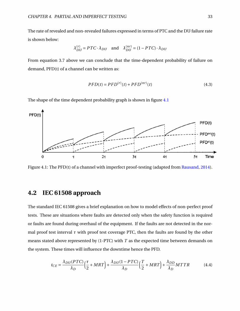
From equation 3.7 above we can conclude that the time-dependent probability of failure on
demand, PFD(t) of a channel can be written as:
PF D(t ) = PF D (r )(t )+PF D (nr )(t ) (4.3)
The shape of the time dependent probability graph is shown in figure 4.1
Figure 4.1: The PFD(t) of a channel with imperfect proof-testing (adapted from Rausand, 2014).
4.2 IEC 61508 approach
The standard IEC 61508 gives a brief explanation on how to model effects of non-perfect proof
tests. These are situations where faults are detected only when the safety function is required
or faults are found during overhaul of the equipment. If the faults are not detected in the nor-
mal proof test interval τ with proof test coverage PTC, then the faults are found by the other
means stated above represented by (1-PTC) with T as the expected time between demands on
the system. These times will influence the downtime hence the PFD.
tC E = λDU (PTC )
λD
(τ2+MRT
)+ λDU (1−PTC )
λD
(T
2+MRT
)+ λDD
λDMT T R (4.4)
CHAPTER 4. PARTIAL AND IMPERFECT TESTING 34
Therefore the PF Dav g given by λD,G · tGE for a 1oo1 channel is:
PF Dav g ≈ PTC ·λDU
(τ2+MRT
)+ (1−PTC ) ·λDU
(T
2+MRT
)+λDD ·MT T R (4.5)
The PF Dav g formula for a 1oo2 configuration is further expressed and clarified in IEC-61508
(2009); Oliveira (2009). The two identical channels with imperfect repair and overhaul is consid-
ered to have a D-fault in 5 different ways namely (i) Two DU faults due to CCF, (ii) Two DD faults
due to CCF, (iii) Two independent DU revealed faults in same proof test interval, (iv) Two inde-
pendent non-revealed faults in the overhaul period and (v) One independent DU revealed fault
and one independent DU non-revealed fault in the same proof test interval (Rausand, 2014).
The IEC PF Dav g for a 1oo2 independent and identical channels is:
PF Dav g =λD,G · tGE = 2(λD )2 · tC E · tGE
Integrating the formulas together gives:
PF D (1oo2)av g = [
(1−β)λDU + (1−βD )λDD]2 · tC E · tGE +PTC ·βλDU
(τ2+MRT
)+ (1−PTC ) ·βλDU
(T
2+MRT
)+βDλDD ·MT T R
(4.6)
where tC E = λrDUλD
(τ2 +MRT
)+ λnr
DUλD
(T2 +MRT
)+ λDD
λDMT T R
and tGE = λrDUλD
(τ3 +MRT
)+ λnr
DUλD
(T3 +MRT
)+ λDD
λDMT T R
4.3 PDS method
The PDS method handbook uses the term critical safety unavailability (CSU) to quantify the loss
of safety. The handbook defines CSU as the probability that a component or system will fail to
automatically carry out a successful safety action on the occurrence of a hazardous event.
C SU = PF D +DTU +PT I F (4.7)
CHAPTER 4. PARTIAL AND IMPERFECT TESTING 35
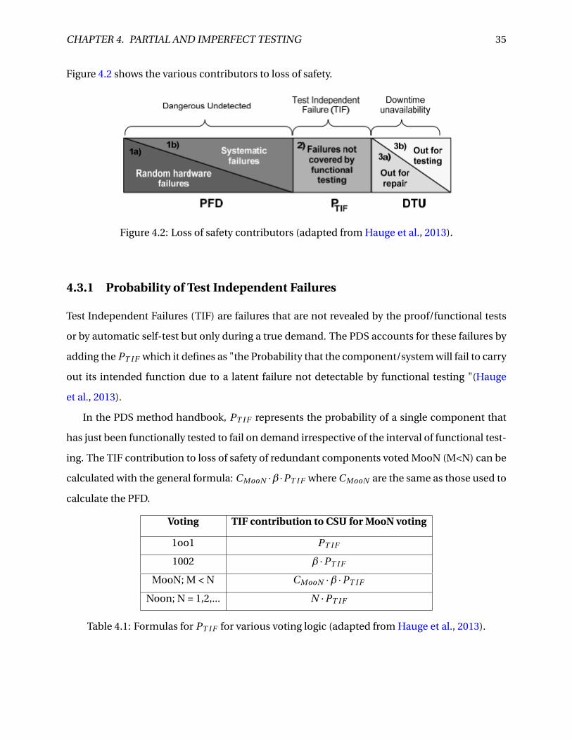
Figure 4.2 shows the various contributors to loss of safety.
Figure 4.2: Loss of safety contributors (adapted from Hauge et al., 2013).
4.3.1 Probability of Test Independent Failures
Test Independent Failures (TIF) are failures that are not revealed by the proof/functional tests
or by automatic self-test but only during a true demand. The PDS accounts for these failures by
adding the PT I F which it defines as "the Probability that the component/system will fail to carry
out its intended function due to a latent failure not detectable by functional testing "(Hauge
et al., 2013).
In the PDS method handbook, PT I F represents the probability of a single component that
has just been functionally tested to fail on demand irrespective of the interval of functional test-
ing. The TIF contribution to loss of safety of redundant components voted MooN (M<N) can be
calculated with the general formula: CMooN ·β ·PT I F where CMooN are the same as those used to
calculate the PFD.
Voting TIF contribution to CSU for MooN voting
1oo1 PT I F
1002 β ·PT I F
MooN; M < N CMooN ·β ·PT I F
Noon; N = 1,2,... N ·PT I F
Table 4.1: Formulas for PT I F for various voting logic (adapted from Hauge et al., 2013).
CHAPTER 4. PARTIAL AND IMPERFECT TESTING 36
4.3.2 Incorporating PTC into PFD Formulas
The PDS handbook also suggests modeling the PTC into PFD formulas as an alternative to the
PT I F in considering imperfect testing. To achieve this, the rate of DU failures is divided into
failures detected during testing with test interval τ and failures not revealed during testing with
interval T which could be a complete component overhaul interval or lifetime of the equipment.
The PFD for a 1oo1 voting considering imperfect testing using the PTC is given as:
PF D1oo1 = PTC ·(λDU · τ
2
)+ (1−PTC ) ·
(λDU · T
2
)(4.8)
Generalizing the PFD formula for any NooN configuration using the standard approximation
gives:
PF DNooN = PTC ·(N ·λDU · τ
2
)+ (1−PTC ) ·
(N ·λDU · T
2
)(4.9)
The common cause contribution for a MooN configuration where a single failure or a CCF is
sufficient for the system to fail is given in equation 4.10 below. Note however that consideration
of independent failures combinations gives more complex equations.
PF DMooN = PTC ·(CMooN ·β ·λDU · τ
2
)+ (1−PTC ) ·
(CMooN ·β ·λDU · T
2
)(4.10)
For a 1oo2 configuration, the contribution by a combination of two independent failures de-
tectable during the function test is added to the first term and the combination of two inde-
pendent failures detectable after time T is added to the second term. Also a contribution from
the combination of one failure detectable in during the function test and one failure detectable
after time T. The system operates as a 1oo1 system for a period when a single failure occurs
which is not detected before time T. As shown in equation 4.11, the second and fourth terms
therefore represent the extensions of two independent failures of same type while the last term
corresponds to a combination of one failure undetectable the function test and one detectable
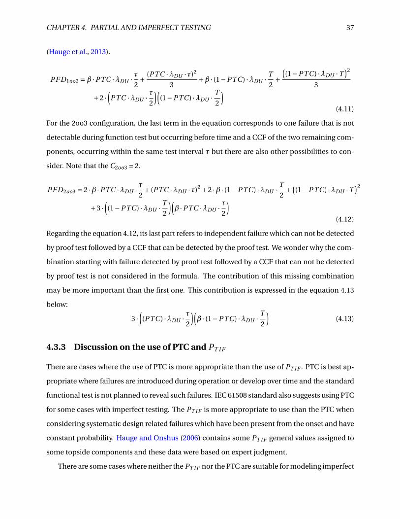
CHAPTER 4. PARTIAL AND IMPERFECT TESTING 37
(Hauge et al., 2013).
PF D1oo2 =β ·PTC ·λDU · τ2+ (PTC ·λDU ·τ)2
3+β · (1−PTC ) ·λDU · T
2+
((1−PTC ) ·λDU ·T
)2
3
+2 ·(PTC ·λDU · τ
2
)((1−PTC ) ·λDU · T
2
)(4.11)
For the 2oo3 configuration, the last term in the equation corresponds to one failure that is not
detectable during function test but occurring before time and a CCF of the two remaining com-
ponents, occurring within the same test interval τ but there are also other possibilities to con-
sider. Note that the C2oo3 = 2.
PF D2oo3 = 2 ·β ·PTC ·λDU · τ2+ (PTC ·λDU ·τ)2 +2 ·β · (1−PTC ) ·λDU · T
2+ (
(1−PTC ) ·λDU ·T)2
+3 ·((1−PTC ) ·λDU · T
2
)(β ·PTC ·λDU · τ
2
)(4.12)
Regarding the equation 4.12, its last part refers to independent failure which can not be detected
by proof test followed by a CCF that can be detected by the proof test. We wonder why the com-
bination starting with failure detected by proof test followed by a CCF that can not be detected
by proof test is not considered in the formula. The contribution of this missing combination
may be more important than the first one. This contribution is expressed in the equation 4.13
below:
3 ·((PTC ) ·λDU · τ
2
)(β · (1−PTC ) ·λDU · T
2
)(4.13)
4.3.3 Discussion on the use of PTC and PT I F
There are cases where the use of PTC is more appropriate than the use of PT I F . PTC is best ap-
propriate where failures are introduced during operation or develop over time and the standard
functional test is not planned to reveal such failures. IEC 61508 standard also suggests using PTC
for some cases with imperfect testing. The PT I F is more appropriate to use than the PTC when
considering systematic design related failures which have been present from the onset and have
constant probability. Hauge and Onshus (2006) contains some PT I F general values assigned to
some topside components and these data were based on expert judgment.
There are some cases where neither the PT I F nor the PTC are suitable for modeling imperfect
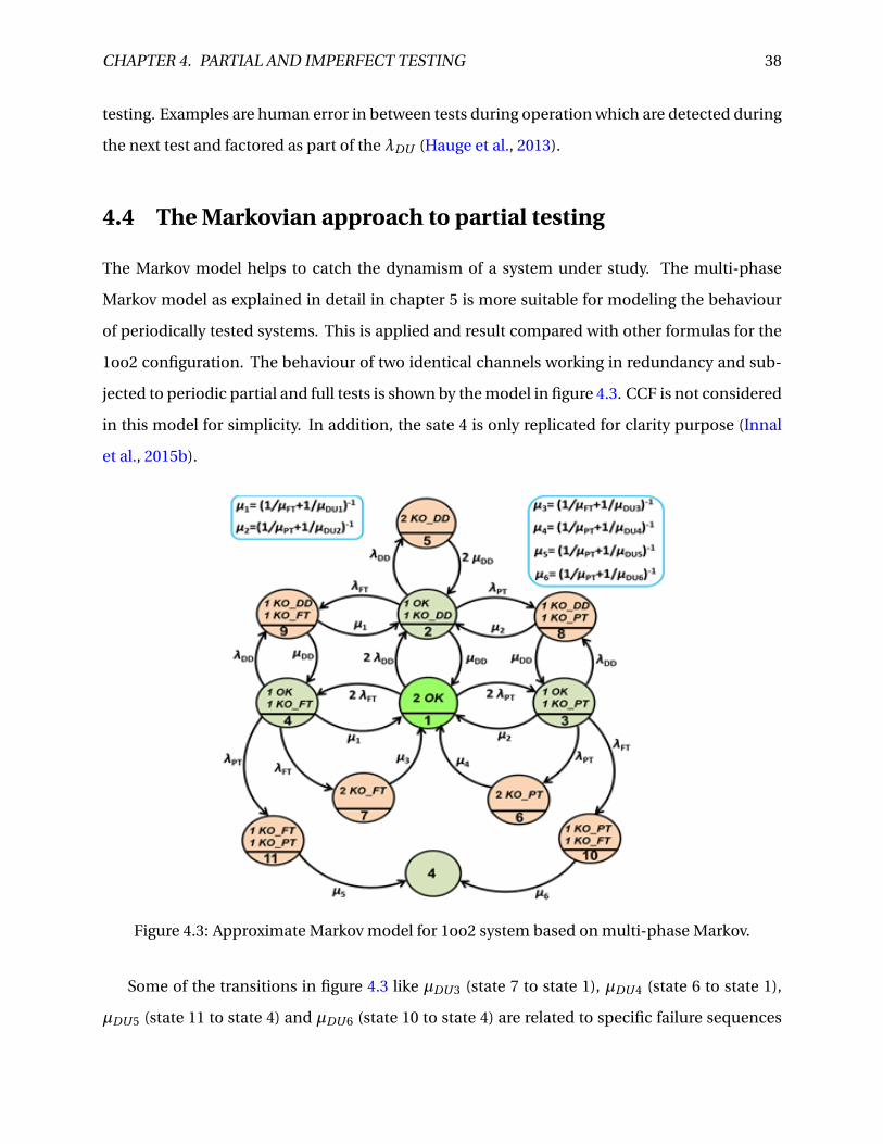
CHAPTER 4. PARTIAL AND IMPERFECT TESTING 38
testing. Examples are human error in between tests during operation which are detected during
the next test and factored as part of the λDU (Hauge et al., 2013).
4.4 The Markovian approach to partial testing
The Markov model helps to catch the dynamism of a system under study. The multi-phase
Markov model as explained in detail in chapter 5 is more suitable for modeling the behaviour
of periodically tested systems. This is applied and result compared with other formulas for the
1oo2 configuration. The behaviour of two identical channels working in redundancy and sub-
jected to periodic partial and full tests is shown by the model in figure 4.3. CCF is not considered
in this model for simplicity. In addition, the sate 4 is only replicated for clarity purpose (Innal
et al., 2015b).
Figure 4.3: Approximate Markov model for 1oo2 system based on multi-phase Markov.
Some of the transitions in figure 4.3 like µDU 3 (state 7 to state 1), µDU 4 (state 6 to state 1),
µDU 5 (state 11 to state 4) and µDU 6 (state 10 to state 4) are related to specific failure sequences
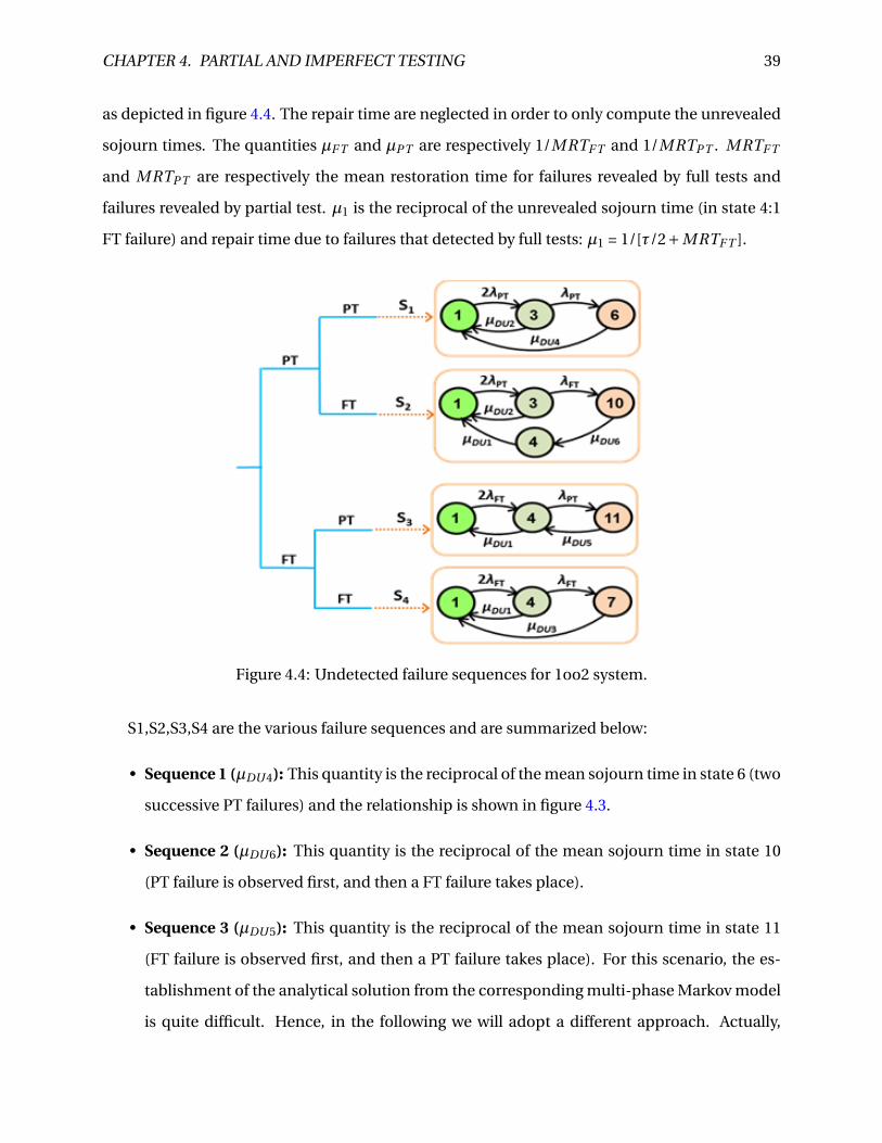
CHAPTER 4. PARTIAL AND IMPERFECT TESTING 39
as depicted in figure 4.4. The repair time are neglected in order to only compute the unrevealed
sojourn times. The quantities µF T and µPT are respectively 1/MRTF T and 1/MRTPT . MRTF T
and MRTPT are respectively the mean restoration time for failures revealed by full tests and
failures revealed by partial test. µ1 is the reciprocal of the unrevealed sojourn time (in state 4:1
FT failure) and repair time due to failures that detected by full tests: µ1 = 1/[τ/2+MRTF T ].
Figure 4.4: Undetected failure sequences for 1oo2 system.
S1,S2,S3,S4 are the various failure sequences and are summarized below:
• Sequence 1 (µDU 4): This quantity is the reciprocal of the mean sojourn time in state 6 (two
successive PT failures) and the relationship is shown in figure 4.3.
• Sequence 2 (µDU 6): This quantity is the reciprocal of the mean sojourn time in state 10
(PT failure is observed first, and then a FT failure takes place).
• Sequence 3 (µDU 5): This quantity is the reciprocal of the mean sojourn time in state 11
(FT failure is observed first, and then a PT failure takes place). For this scenario, the es-
tablishment of the analytical solution from the corresponding multi-phase Markov model
is quite difficult. Hence, in the following we will adopt a different approach. Actually,
CHAPTER 4. PARTIAL AND IMPERFECT TESTING 40
the mean unavailability to the combination of FT and PT failures (whatever their order of
occurrence: states 10 and 11) could be easily obtained.
• Sequence 4 (µDU 3): This quantity is the reciprocal of the mean sojourn time in state 7 (two
successive FT failures).
The complete process of these repair rates is given in (Innal et al., 2015b). The PF Dav g for the
1oo2 system based on the Markov model in figure 4.3 can be calculated as:
PF D1oo2av g =
11∑i=5
Pi (∞) (4.14)
The steady-state probabilities based on substitutions and approximations for the different states
are given as:
P1(∞) ≈ 1;P2(∞) ≈ 2λDD
µDD;P3(∞) ≈ 2λPT
µ2;P4(∞) ≈ 2λF T
µ1;P5(∞) ≈ 2λ2
DD
2µ2DD
;P6(∞) ≈ 2λ2PT
µ2µ4;
P7(∞) ≈ 2λ2F T
µ1µ3;P8(∞) ≈ 2λPTλDD
µ2µDD;P9(∞) ≈ 2λF TλDD
µ1µDD;P10(∞) ≈ 2λPTλF T
µ2µ6;P11(∞) ≈ 2λF TλPT
µ1µ5;
Therefore the PF Dav g can be calculated thus:
PF D1oo2av g = 2λPT
µ1·(λF T
µ6+ λPT
µ4+ λDD
µDD
)+ 2λF T
µ1·(λF T
µ3+ λPT
µ5+ λDD
µDD
)+ λ2
DD
µ2DD
(4.15)
The mean downtime MDT1oo2 is given by PF D1oo2av g /PF H1oo2 which is expressed as:
MDT1oo2 ≈P3(∞)
(λF Tµ6
+ λPTµ4
+ λDDµDD
)+P4(∞)
(λF Tµ3
+ λPTµ5
+ λDDµDD
)λD
[P3(∞)+P4(∞)
] (4.16)
The MDT1oo2 given in Oliveira (2009); Rausand (2014); IEC-61508 (2009) expressed in equation
in section 4.2 above can be re-written as:
MDT1oo2 ≈ 1
λD
(λF T
µ3+ λPT
µ4+ λDD
µDD
)(4.17)
Equations 4.15 and 4.16 would be the same if µ5 = µ4 and µ6 = µ3. Therefore in the PF D1oo2av g
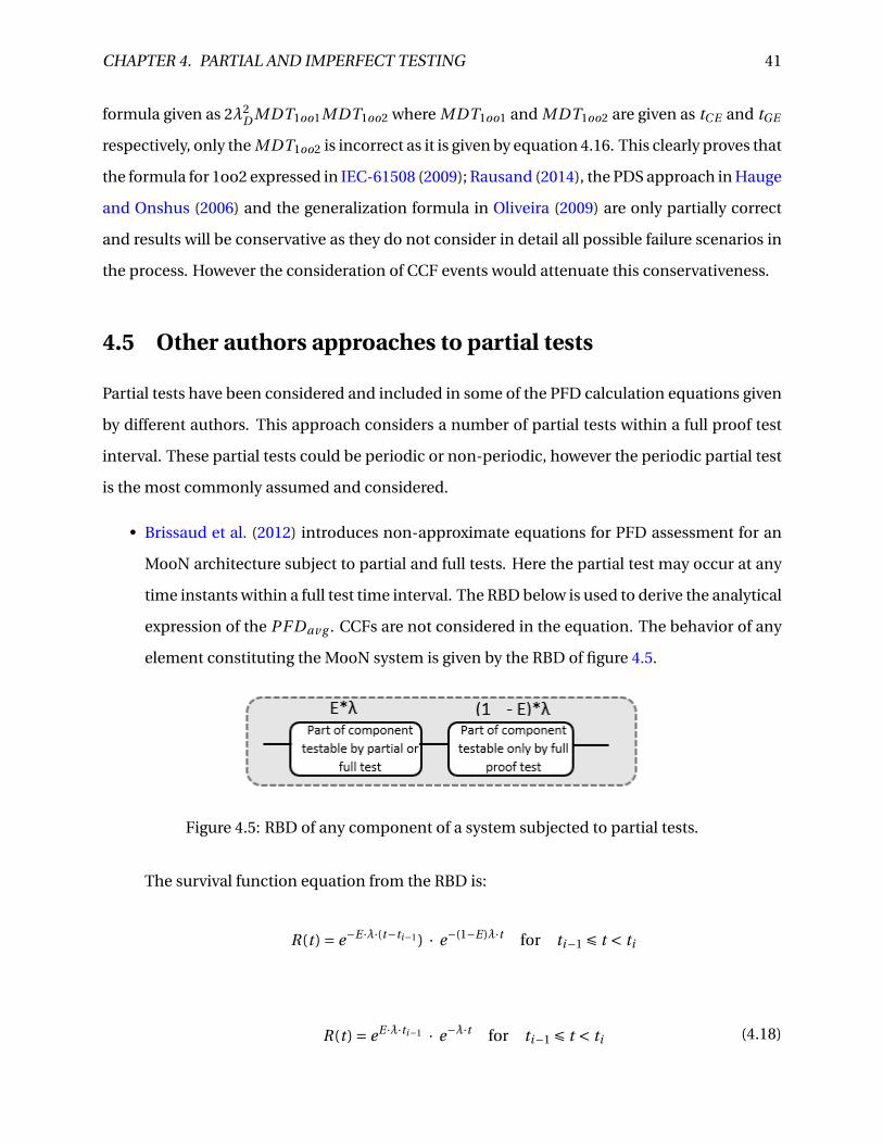
CHAPTER 4. PARTIAL AND IMPERFECT TESTING 41
formula given as 2λ2D MDT1oo1MDT1oo2 where MDT1oo1 and MDT1oo2 are given as tC E and tGE
respectively, only the MDT1oo2 is incorrect as it is given by equation 4.16. This clearly proves that
the formula for 1oo2 expressed in IEC-61508 (2009); Rausand (2014), the PDS approach in Hauge
and Onshus (2006) and the generalization formula in Oliveira (2009) are only partially correct
and results will be conservative as they do not consider in detail all possible failure scenarios in
the process. However the consideration of CCF events would attenuate this conservativeness.
4.5 Other authors approaches to partial tests
Partial tests have been considered and included in some of the PFD calculation equations given
by different authors. This approach considers a number of partial tests within a full proof test
interval. These partial tests could be periodic or non-periodic, however the periodic partial test
is the most commonly assumed and considered.
• Brissaud et al. (2012) introduces non-approximate equations for PFD assessment for an
MooN architecture subject to partial and full tests. Here the partial test may occur at any
time instants within a full test time interval. The RBD below is used to derive the analytical
expression of the PF Dav g . CCFs are not considered in the equation. The behavior of any
element constituting the MooN system is given by the RBD of figure 4.5.
Figure 4.5: RBD of any component of a system subjected to partial tests.
The survival function equation from the RBD is:
R(t ) = e−E ·λ·(t−ti−1 ) · e−(1−E)λ·t for ti−1 É t < ti
R(t ) = eE ·λ·ti−1 · e−λ·t for ti−1 É t < ti (4.18)
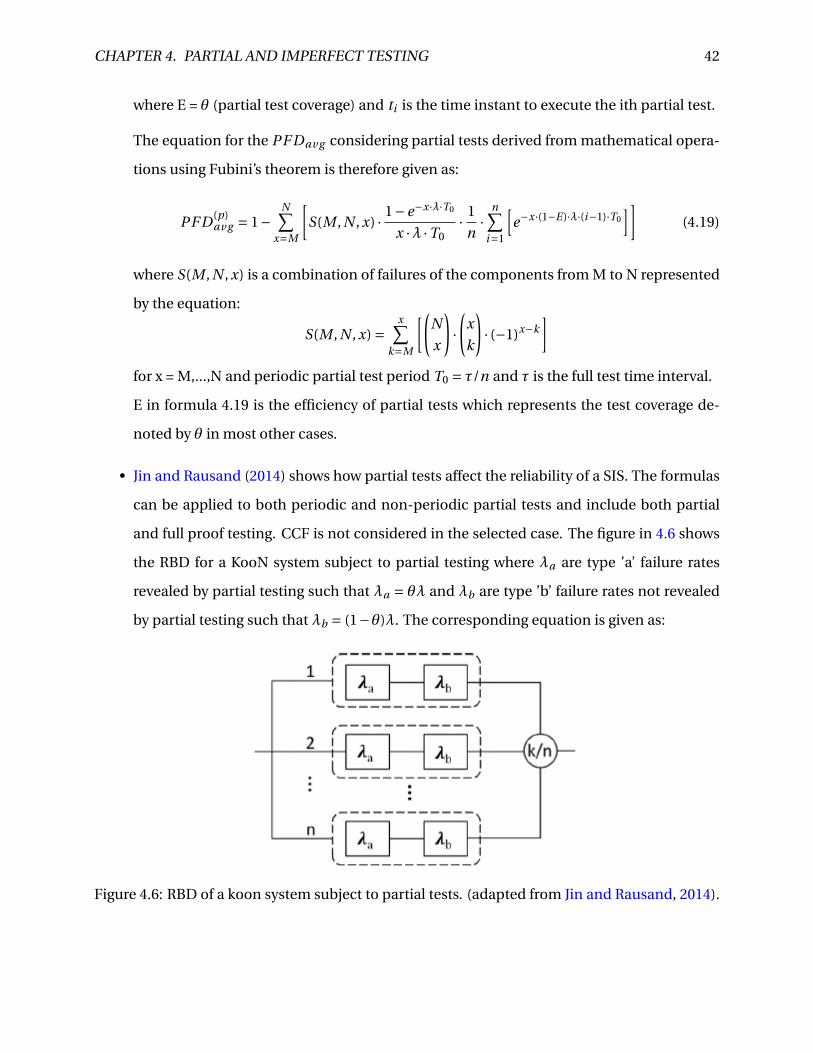
CHAPTER 4. PARTIAL AND IMPERFECT TESTING 42
where E = θ (partial test coverage) and ti is the time instant to execute the ith partial test.
The equation for the PF Dav g considering partial tests derived from mathematical opera-
tions using Fubini’s theorem is therefore given as:
PF D (p)av g = 1−
N∑x=M
[S(M , N , x) · 1−e−x·λ·T0
x ·λ ·T0· 1
n·
n∑i=1
[e−x·(1−E)·λ·(i−1)·T0
]](4.19)
where S(M , N , x) is a combination of failures of the components from M to N represented
by the equation:
S(M , N , x) =x∑
k=M
[(N
x
)·(
x
k
)· (−1)x−k
]for x = M,...,N and periodic partial test period T0 = τ/n and τ is the full test time interval.
E in formula 4.19 is the efficiency of partial tests which represents the test coverage de-
noted by θ in most other cases.
• Jin and Rausand (2014) shows how partial tests affect the reliability of a SIS. The formulas
can be applied to both periodic and non-periodic partial tests and include both partial
and full proof testing. CCF is not considered in the selected case. The figure in 4.6 shows
the RBD for a KooN system subject to partial testing where λa are type ’a’ failure rates
revealed by partial testing such that λa = θλ and λb are type ’b’ failure rates not revealed
by partial testing such that λb = (1−θ)λ. The corresponding equation is given as:
Figure 4.6: RBD of a koon system subject to partial tests. (adapted from Jin and Rausand, 2014).
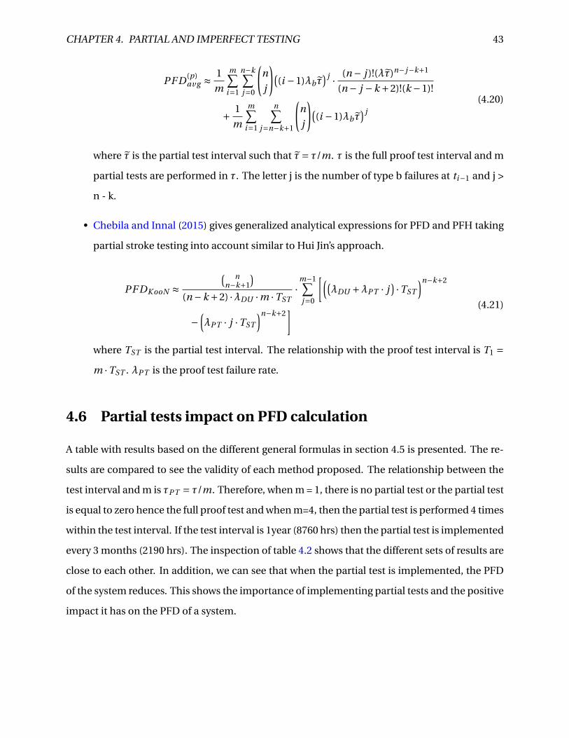
CHAPTER 4. PARTIAL AND IMPERFECT TESTING 43
PF D (p)av g ≈ 1
m
m∑i=1
n−k∑j=0
(n
j
)((i −1)λb τ̃
) j · (n − j )!(λτ̃)n− j−k+1
(n − j −k +2)!(k −1)!
+ 1
m
m∑i=1
n∑j=n−k+1
(n
j
)((i −1)λb τ̃
) j
(4.20)
where τ̃ is the partial test interval such that τ̃= τ/m. τ is the full proof test interval and m
partial tests are performed in τ. The letter j is the number of type b failures at ti−1 and j >
n - k.
• Chebila and Innal (2015) gives generalized analytical expressions for PFD and PFH taking
partial stroke testing into account similar to Hui Jin’s approach.
PF DK ooN ≈( n
n−k+1
)(n −k +2) ·λDU ·m ·TST
·m−1∑j=0
[((λDU +λPT · j
) ·TST
)n−k+2
−(λPT · j ·TST
)n−k+2] (4.21)
where TST is the partial test interval. The relationship with the proof test interval is T1 =m ·TST . λPT is the proof test failure rate.
4.6 Partial tests impact on PFD calculation
A table with results based on the different general formulas in section 4.5 is presented. The re-
sults are compared to see the validity of each method proposed. The relationship between the
test interval and m is τPT = τ/m. Therefore, when m = 1, there is no partial test or the partial test
is equal to zero hence the full proof test and when m=4, then the partial test is performed 4 times
within the test interval. If the test interval is 1year (8760 hrs) then the partial test is implemented
every 3 months (2190 hrs). The inspection of table 4.2 shows that the different sets of results are
close to each other. In addition, we can see that when the partial test is implemented, the PFD
of the system reduces. This shows the importance of implementing partial tests and the positive
impact it has on the PFD of a system.
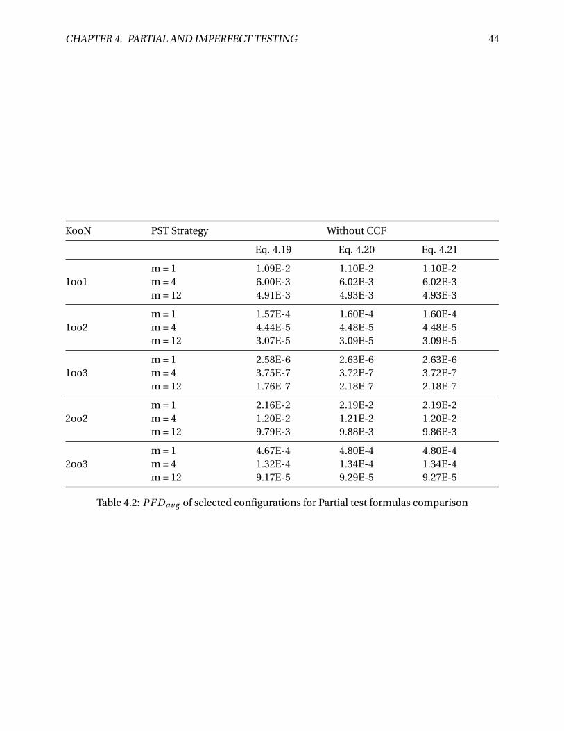
CHAPTER 4. PARTIAL AND IMPERFECT TESTING 44
KooN PST Strategy Without CCF
Eq. 4.19 Eq. 4.20 Eq. 4.21
1oo1m = 1 1.09E-2 1.10E-2 1.10E-2m = 4 6.00E-3 6.02E-3 6.02E-3m = 12 4.91E-3 4.93E-3 4.93E-3
1oo2m = 1 1.57E-4 1.60E-4 1.60E-4m = 4 4.44E-5 4.48E-5 4.48E-5m = 12 3.07E-5 3.09E-5 3.09E-5
1oo3m = 1 2.58E-6 2.63E-6 2.63E-6m = 4 3.75E-7 3.72E-7 3.72E-7m = 12 1.76E-7 2.18E-7 2.18E-7
2oo2m = 1 2.16E-2 2.19E-2 2.19E-2m = 4 1.20E-2 1.21E-2 1.20E-2m = 12 9.79E-3 9.88E-3 9.86E-3
2oo3m = 1 4.67E-4 4.80E-4 4.80E-4m = 4 1.32E-4 1.34E-4 1.34E-4m = 12 9.17E-5 9.29E-5 9.27E-5
Table 4.2: PF Dav g of selected configurations for Partial test formulas comparison

Chapter 5
Verification of Analytical formulas for
testing
5.1 Phased Markov for periodically tested components
Reliability assessment methods like the RBD and FTA only consider a system’s functioning and
failed state. To be able to model other states of a system like the degraded state, Markov analysis
is ideal. Markov analysis considers different system states, transition between the states and the
rate at which the transitions occur. The Markov property is a stochastic process where the future
state only depends on the present, and not the past.
Pr (X (t + s) = j | X (t ) = i , X (u) = i , X (u) = x(u),0 ≤ u < s) = Pr (X (t + s) = j | X (s) = i
The standard Markov chain has some limitations which makes it difficult to correctly model the
behavior of periodically and partially tested SIS with several periods. This test behavior requires
the use of a multi-phase Markov Chain (Dutuit et al., 2008; Mechri et al., 2013). IEC 61508 sug-
gests a multi-phased Markovian approach to model such systems. Multi-phase Markov chains
are appropriate for modeling changes in structure of the states at known instants or when the
state of some parts of the system are known at some instants. The latter case is proof testing
which creates a new phase in the Markov chain evolution. Figure 5.1 shows that the normal
Markov process on the upper part of the figure represents a single component which can fail
45
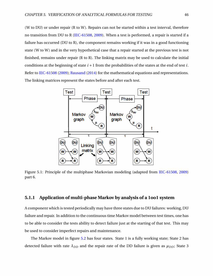
CHAPTER 5. VERIFICATION OF ANALYTICAL FORMULAS FOR TESTING 46
(W to DU) or under repair (R to W). Repairs can not be started within a test interval, therefore
no transition from DU to R (IEC-61508, 2009). When a test is performed, a repair is started if a
failure has occurred (DU to R), the component remains working if it was in a good functioning
state (W to W) and in the very hypothetical case that a repair started at the previous test is not
finished, remains under repair (R to R). The linking matrix may be used to calculate the initial
conditions at the beginning of state i +1 from the probabilities of the states at the end of test i .
Refer to IEC-61508 (2009); Rausand (2014) for the mathematical equations and representations.
The linking matrices represent the states before and after each test.
Figure 5.1: Principle of the multiphase Markovian modeling (adapted from IEC-61508, 2009)part 6.
5.1.1 Application of multi-phase Markov by analysis of a 1oo1 system
A component which is tested periodically may have three states due to DU failures: working, DU
failure and repair. In addition to the continuous time Markov model between test times, one has
to be able to consider the tests ability to detect failure just at the starting of that test. This may
be used to consider imperfect repairs and maintenance.
The Markov model in figure 5.2 has four states. State 1 is a fully working state; State 2 has
detected failure with rate λDD and the repair rate of the DD failure is given as µDD ; State 3
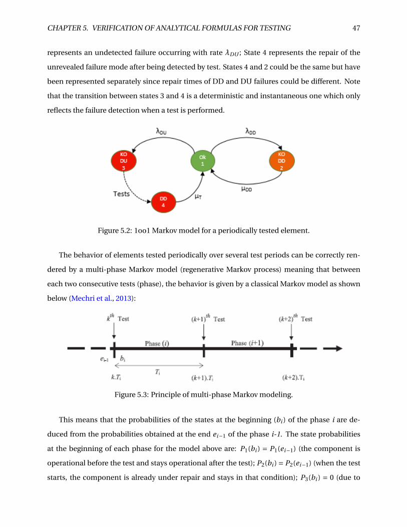
CHAPTER 5. VERIFICATION OF ANALYTICAL FORMULAS FOR TESTING 47
represents an undetected failure occurring with rate λDU ; State 4 represents the repair of the
unrevealed failure mode after being detected by test. States 4 and 2 could be the same but have
been represented separately since repair times of DD and DU failures could be different. Note
that the transition between states 3 and 4 is a deterministic and instantaneous one which only
reflects the failure detection when a test is performed.
Figure 5.2: 1oo1 Markov model for a periodically tested element.
The behavior of elements tested periodically over several test periods can be correctly ren-
dered by a multi-phase Markov model (regenerative Markov process) meaning that between
each two consecutive tests (phase), the behavior is given by a classical Markov model as shown
below (Mechri et al., 2013):
Figure 5.3: Principle of multi-phase Markov modeling.
This means that the probabilities of the states at the beginning (bi ) of the phase i are de-
duced from the probabilities obtained at the end ei−1 of the phase i-1. The state probabilities
at the beginning of each phase for the model above are: P1(bi ) = P1(ei−1) (the component is
operational before the test and stays operational after the test); P2(bi ) = P2(ei−1) (when the test
starts, the component is already under repair and stays in that condition); P3(bi ) = 0 (due to
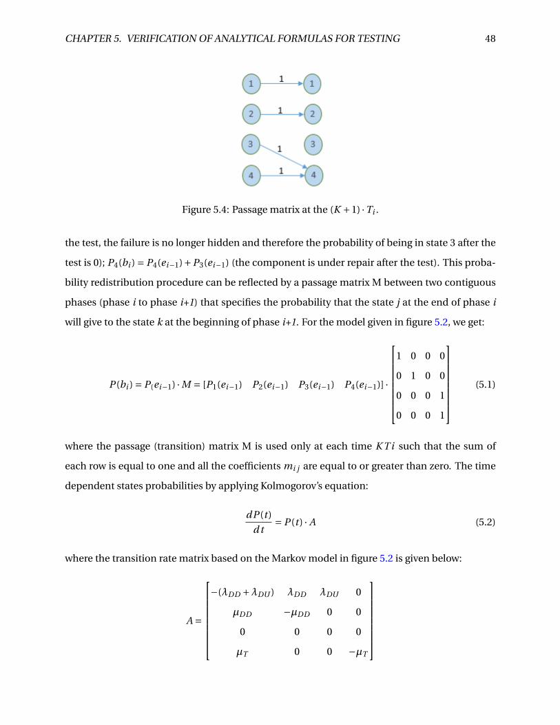
CHAPTER 5. VERIFICATION OF ANALYTICAL FORMULAS FOR TESTING 48
Figure 5.4: Passage matrix at the (K +1) ·Ti .
the test, the failure is no longer hidden and therefore the probability of being in state 3 after the
test is 0); P4(bi ) = P4(ei−1)+P3(ei−1) (the component is under repair after the test). This proba-
bility redistribution procedure can be reflected by a passage matrix M between two contiguous
phases (phase i to phase i+1) that specifies the probability that the state j at the end of phase i
will give to the state k at the beginning of phase i+1. For the model given in figure 5.2, we get:
P (bi ) = P(ei−1) ·M = [P1(ei−1) P2(ei−1) P3(ei−1) P4(ei−1)] ·
1 0 0 0
0 1 0 0
0 0 0 1
0 0 0 1
(5.1)
where the passage (transition) matrix M is used only at each time K T i such that the sum of
each row is equal to one and all the coefficients mi j are equal to or greater than zero. The time
dependent states probabilities by applying Kolmogorov’s equation:
dP (t )
d t= P (t ) · A (5.2)
where the transition rate matrix based on the Markov model in figure 5.2 is given below:
A =
−(λDD +λDU ) λDD λDU 0
µDD −µDD 0 0
0 0 0 0
µT 0 0 −µT
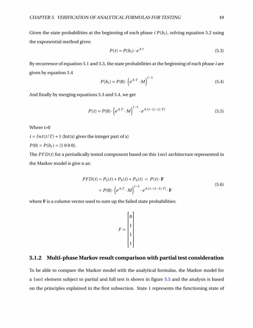
CHAPTER 5. VERIFICATION OF ANALYTICAL FORMULAS FOR TESTING 49
Given the state probabilities at the beginning of each phase i P (bi ), solving equation 5.2 using
the exponential method gives:
P (t ) = P (bi ) ·e A·t (5.3)
By recurrence of equation 5.1 and 5.3, the state probabilities at the beginning of each phase i are
given by equation 5.4
P (bi ) = P (0) ·(e A·T ·M
)i−1(5.4)
And finally by merging equations 5.3 and 5.4, we get
P (t ) = P (0) ·(e A·T ·M
)i−1·e A·[t−(i−1)·T ] (5.5)
Where t>0
i = lnt (t/T )+1 (lnt(x) gives the integer part of x)
P (0) = P (b1) = [1 0 0 0].
The PF D(t ) for a periodically tested component based on this 1oo1 architecture represented in
the Markov model is give n as:
PF D(t ) = P2(t )+P3(t )+P4(t ) = P (t ) ·F
= P (0) ·(e A·T ·M
)i−1·e A·[t−(i−1)·T ] ·F
(5.6)
where F is a column vector used to sum up the failed state probabilities:
F =
0
1
1
1
5.1.2 Multi-phase Markov result comparison with partial test consideration
To be able to compare the Markov model with the analytical formulas, the Markov model for
a 1oo1 element subject to partial and full test is shown in figure 5.5 and the analysis is based
on the principles explained in the first subsection. State 1 represents the functioning state of
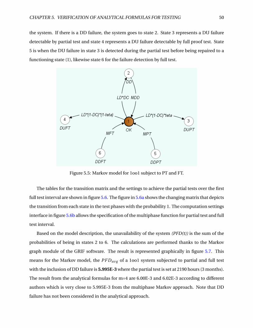
CHAPTER 5. VERIFICATION OF ANALYTICAL FORMULAS FOR TESTING 50
the system. If there is a DD failure, the system goes to state 2. State 3 represents a DU failure
detectable by partial test and state 4 represents a DU failure detectable by full proof test. State
5 is when the DU failure in state 3 is detected during the partial test before being repaired to a
functioning state (1), likewise state 6 for the failure detection by full test.
Figure 5.5: Markov model for 1oo1 subject to PT and FT.
The tables for the transition matrix and the settings to achieve the partial tests over the first
full test interval are shown in figure 5.6. The figure in 5.6a shows the changing matrix that depicts
the transition from each state in the test phases with the probability 1. The computation settings
interface in figure 5.6b allows the specification of the multiphase function for partial test and full
test interval.
Based on the model description, the unavailability of the system (PFD(t)) is the sum of the
probabilities of being in states 2 to 6. The calculations are performed thanks to the Markov
graph module of the GRIF software. The result is represented graphically in figure 5.7. This
means for the Markov model, the PF Dav g of a 1oo1 system subjected to partial and full test
with the inclusion of DD failure is 5.995E-3 where the partial test is set at 2190 hours (3 months).
The result from the analytical formulas for m=4 are 6.00E-3 and 6.02E-3 according to different
authors which is very close to 5.995E-3 from the multiphase Markov approach. Note that DD
failure has not been considered in the analytical approach.
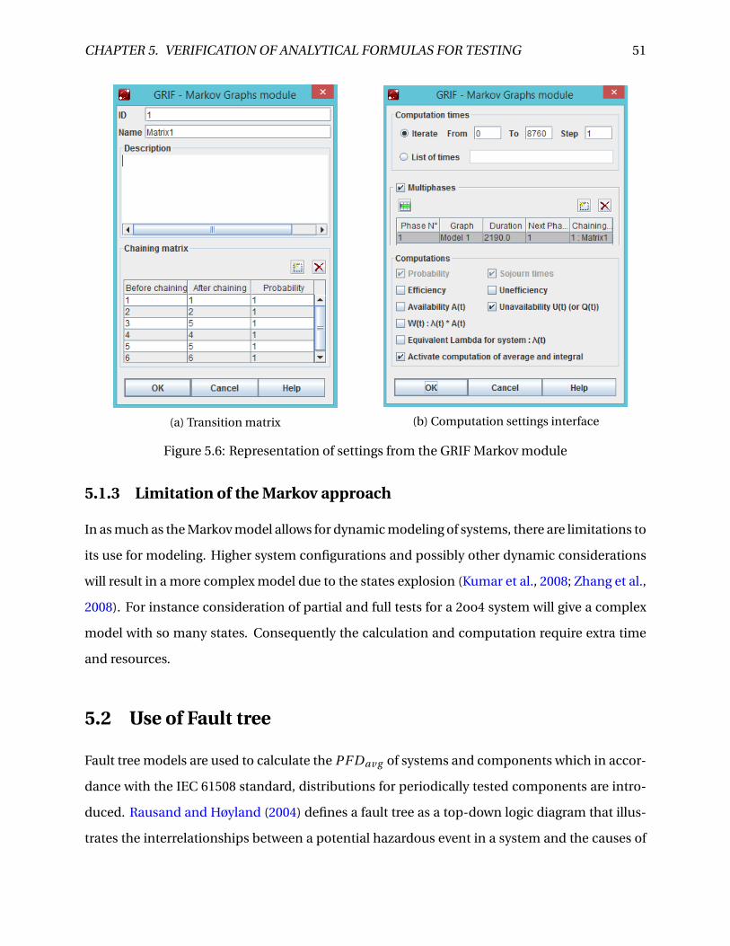
CHAPTER 5. VERIFICATION OF ANALYTICAL FORMULAS FOR TESTING 51
(a) Transition matrix (b) Computation settings interface
Figure 5.6: Representation of settings from the GRIF Markov module
5.1.3 Limitation of the Markov approach
In as much as the Markov model allows for dynamic modeling of systems, there are limitations to
its use for modeling. Higher system configurations and possibly other dynamic considerations
will result in a more complex model due to the states explosion (Kumar et al., 2008; Zhang et al.,
2008). For instance consideration of partial and full tests for a 2oo4 system will give a complex
model with so many states. Consequently the calculation and computation require extra time
and resources.
5.2 Use of Fault tree
Fault tree models are used to calculate the PF Dav g of systems and components which in accor-
dance with the IEC 61508 standard, distributions for periodically tested components are intro-
duced. Rausand and Høyland (2004) defines a fault tree as a top-down logic diagram that illus-
trates the interrelationships between a potential hazardous event in a system and the causes of
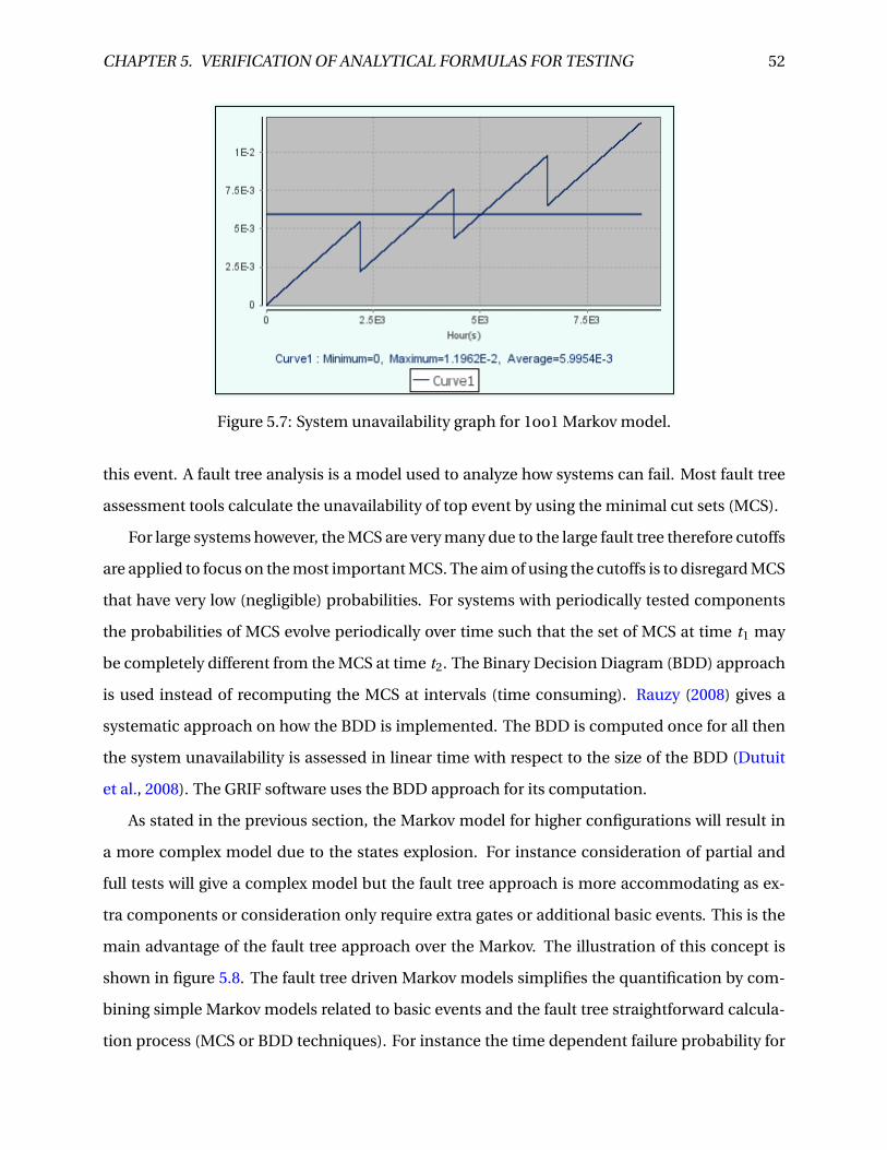
CHAPTER 5. VERIFICATION OF ANALYTICAL FORMULAS FOR TESTING 52
Figure 5.7: System unavailability graph for 1oo1 Markov model.
this event. A fault tree analysis is a model used to analyze how systems can fail. Most fault tree
assessment tools calculate the unavailability of top event by using the minimal cut sets (MCS).
For large systems however, the MCS are very many due to the large fault tree therefore cutoffs
are applied to focus on the most important MCS. The aim of using the cutoffs is to disregard MCS
that have very low (negligible) probabilities. For systems with periodically tested components
the probabilities of MCS evolve periodically over time such that the set of MCS at time t1 may
be completely different from the MCS at time t2. The Binary Decision Diagram (BDD) approach
is used instead of recomputing the MCS at intervals (time consuming). Rauzy (2008) gives a
systematic approach on how the BDD is implemented. The BDD is computed once for all then
the system unavailability is assessed in linear time with respect to the size of the BDD (Dutuit
et al., 2008). The GRIF software uses the BDD approach for its computation.
As stated in the previous section, the Markov model for higher configurations will result in
a more complex model due to the states explosion. For instance consideration of partial and
full tests will give a complex model but the fault tree approach is more accommodating as ex-
tra components or consideration only require extra gates or additional basic events. This is the
main advantage of the fault tree approach over the Markov. The illustration of this concept is
shown in figure 5.8. The fault tree driven Markov models simplifies the quantification by com-
bining simple Markov models related to basic events and the fault tree straightforward calcula-
tion process (MCS or BDD techniques). For instance the time dependent failure probability for
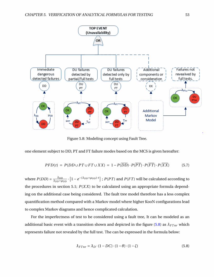
CHAPTER 5. VERIFICATION OF ANALYTICAL FORMULAS FOR TESTING 53
Figure 5.8: Modeling concept using Fault Tree.
one element subject to DD, PT and FT failure modes based on the MCS is given hereafter:
PF D(t ) = P (DD ∪PT ∪F T ∪X X ) = 1−P (DD) ·P (PT ) ·P (F T ) ·P (X X ) (5.7)
where P (DD) = λDDλDD+µDD
· [1− e−(λDD+µDD )·t ] ; P (PT ) and P (F T ) will be calculated according to
the procedures in section 5.1; P (X X ) to be calculated using an appropriate formula depend-
ing on the additional case being considered. The fault tree model therefore has a less complex
quantification method compared with a Markov model where higher KooN configurations lead
to complex Markov diagrams and hence complicated calculation.
For the imperfectness of test to be considered using a fault tree, It can be modeled as an
additional basic event with a transition shown and depicted in the figure (5.8) as λF T nr which
represents failure not revealed by the full test. The can be expressed in the formula below:
λF T nr =λD · (1−DC ) · (1−θ) · (1−ξ) (5.8)
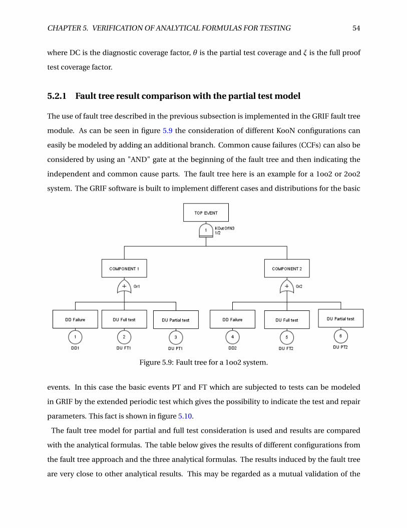
CHAPTER 5. VERIFICATION OF ANALYTICAL FORMULAS FOR TESTING 54
where DC is the diagnostic coverage factor, θ is the partial test coverage and ξ is the full proof
test coverage factor.
5.2.1 Fault tree result comparison with the partial test model
The use of fault tree described in the previous subsection is implemented in the GRIF fault tree
module. As can be seen in figure 5.9 the consideration of different KooN configurations can
easily be modeled by adding an additional branch. Common cause failures (CCFs) can also be
considered by using an "AND" gate at the beginning of the fault tree and then indicating the
independent and common cause parts. The fault tree here is an example for a 1oo2 or 2oo2
system. The GRIF software is built to implement different cases and distributions for the basic
Figure 5.9: Fault tree for a 1oo2 system.
events. In this case the basic events PT and FT which are subjected to tests can be modeled
in GRIF by the extended periodic test which gives the possibility to indicate the test and repair
parameters. This fact is shown in figure 5.10.
The fault tree model for partial and full test consideration is used and results are compared
with the analytical formulas. The table below gives the results of different configurations from
the fault tree approach and the three analytical formulas. The results induced by the fault tree
are very close to other analytical results. This may be regarded as a mutual validation of the
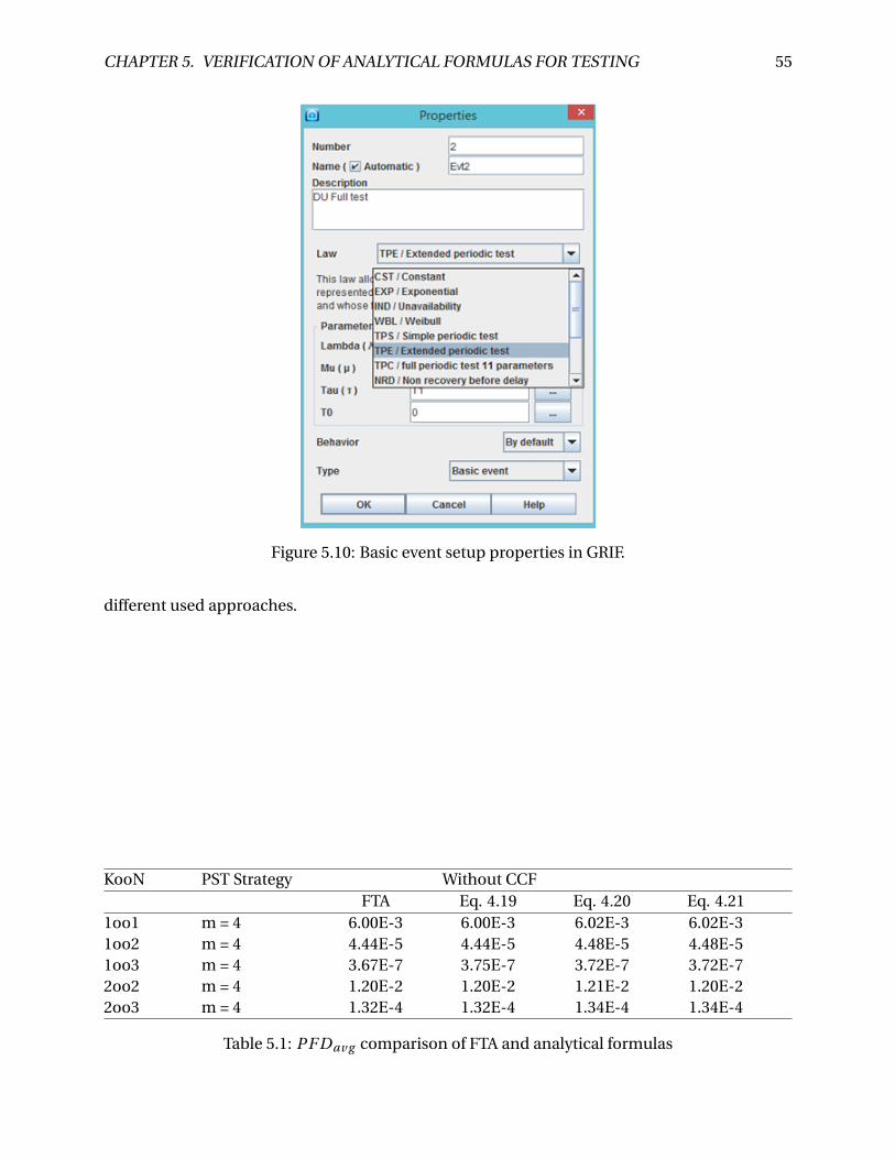
CHAPTER 5. VERIFICATION OF ANALYTICAL FORMULAS FOR TESTING 55
Figure 5.10: Basic event setup properties in GRIF.
different used approaches.
KooN PST Strategy Without CCFFTA Eq. 4.19 Eq. 4.20 Eq. 4.21
1oo1 m = 4 6.00E-3 6.00E-3 6.02E-3 6.02E-31oo2 m = 4 4.44E-5 4.44E-5 4.48E-5 4.48E-51oo3 m = 4 3.67E-7 3.75E-7 3.72E-7 3.72E-72oo2 m = 4 1.20E-2 1.20E-2 1.21E-2 1.20E-22oo3 m = 4 1.32E-4 1.32E-4 1.34E-4 1.34E-4
Table 5.1: PF Dav g comparison of FTA and analytical formulas
Chapter 6
Petri Net
6.1 Introduction to Petri Nets
The Petri net modeling approach was introduced by Carl Adam Petri and IEC 61508 part 6 sug-
gest it as a suitable approach for reliability analysis. IEC standard 62551 defines the terminolo-
gies and gives requirements for the use of Petri net modeling in reliability analysis. The Petri net
approach is similar to the Markov approach based on the possible system states and how they
change when events occur (Rausand, 2014).
6.1.1 Concepts of Petri nets
A typical Petri net model consists of places represented by circles and transitions represented by
a bar or rectangle. The directed arcs are arrows that connect the places and the transitions. The
places, transitions and the oriented arcs are the static part of a PN. Tokens represented by black
bullets are assigned to places to indicate the status/properties of the place. A place is considered
active if it contains a token but it some cases may need more than one token to be considered
active. Marking is a term used to describe the distribution of tokens in the places of the PN
model. Firing a transition enables the movement of a token from place to place (David and Alla,
2010). Transitions could be guarded by deterministic values (e.g. delay); stochastic variables
(e.g. random value according to a probability distribution); conditional statements (predicates,
guards) and arc constrains (e.g., weights or inhibitors) (Aguilar Martinez, 2014). An inhibitor arc
56
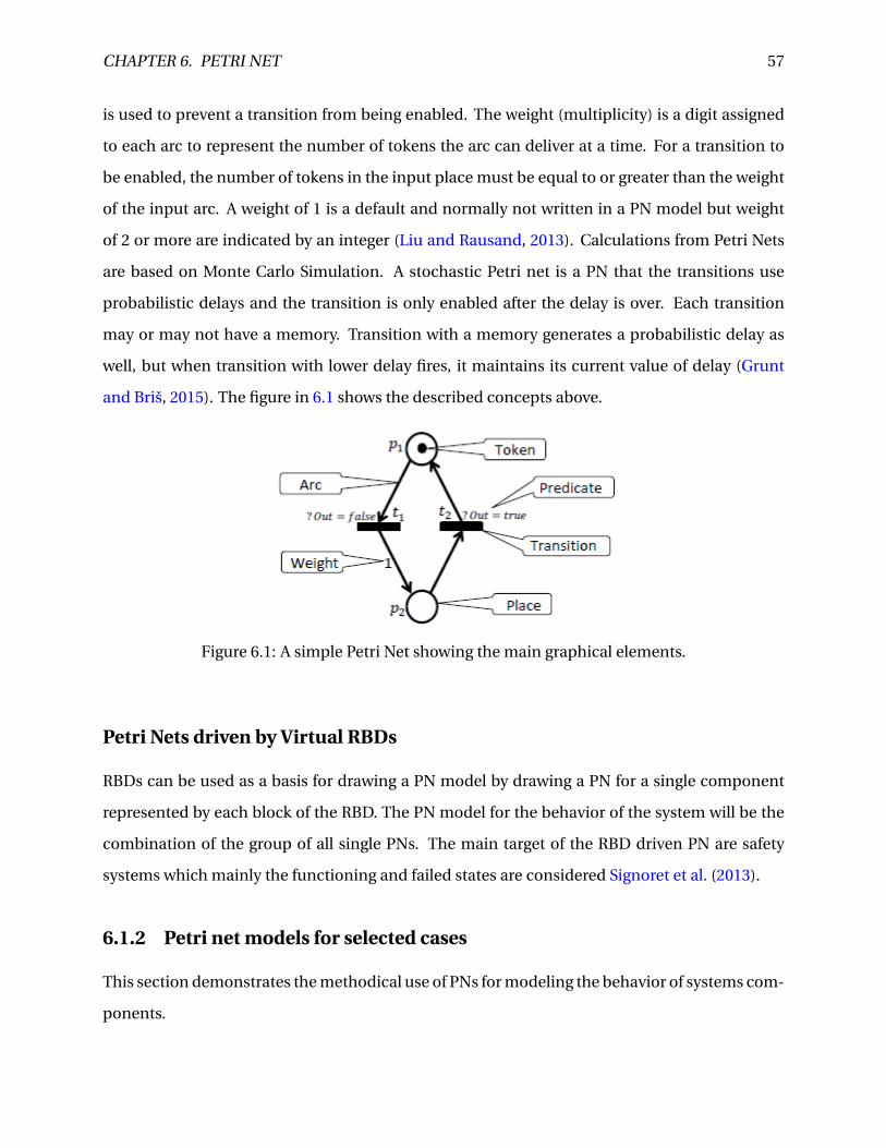
CHAPTER 6. PETRI NET 57
is used to prevent a transition from being enabled. The weight (multiplicity) is a digit assigned
to each arc to represent the number of tokens the arc can deliver at a time. For a transition to
be enabled, the number of tokens in the input place must be equal to or greater than the weight
of the input arc. A weight of 1 is a default and normally not written in a PN model but weight
of 2 or more are indicated by an integer (Liu and Rausand, 2013). Calculations from Petri Nets
are based on Monte Carlo Simulation. A stochastic Petri net is a PN that the transitions use
probabilistic delays and the transition is only enabled after the delay is over. Each transition
may or may not have a memory. Transition with a memory generates a probabilistic delay as
well, but when transition with lower delay fires, it maintains its current value of delay (Grunt
and Briš, 2015). The figure in 6.1 shows the described concepts above.
Figure 6.1: A simple Petri Net showing the main graphical elements.
Petri Nets driven by Virtual RBDs
RBDs can be used as a basis for drawing a PN model by drawing a PN for a single component
represented by each block of the RBD. The PN model for the behavior of the system will be the
combination of the group of all single PNs. The main target of the RBD driven PN are safety
systems which mainly the functioning and failed states are considered Signoret et al. (2013).
6.1.2 Petri net models for selected cases
This section demonstrates the methodical use of PNs for modeling the behavior of systems com-
ponents.
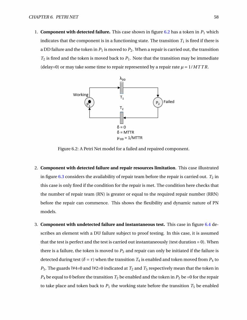
CHAPTER 6. PETRI NET 58
1. Component with detected failure. This case shown in figure 6.2 has a token in P1 which
indicates that the component is in a functioning state. The transition T1 is fired if there is
a DD failure and the token in P1 is moved to P2. When a repair is carried out, the transition
T2 is fired and the token is moved back to P1. Note that the transition may be immediate
(delay=0) or may take some time to repair represented by a repair rate µ= 1/MT T R.
Figure 6.2: A Petri Net model for a failed and repaired component.
2. Component with detected failure and repair resources limitation. This case illustrated
in figure 6.3 considers the availability of repair team before the repair is carried out. T2 in
this case is only fired if the condition for the repair is met. The condition here checks that
the number of repair team (RN) is greater or equal to the required repair number (RRN)
before the repair can commence. This shows the flexibility and dynamic nature of PN
models.
3. Component with undetected failure and instantaneous test. This case in figure 6.4 de-
scribes an element with a DU failure subject to proof testing. In this case, it is assumed
that the test is perfect and the test is carried out instantaneously (test duration = 0). When
there is a failure, the token is moved to P2 and repair can only be initiated if the failure is
detected during test (δ= τ) when the transition T4 is enabled and token moved from P4 to
P5. The guards ?#4=0 and ?#2=0 indicated at T2 and T5 respectively mean that the token in
P4 be equal to 0 before the transition T2 be enabled and the token in P2 be =0 for the repair
to take place and token back to P1 the working state before the transition T5 be enabled
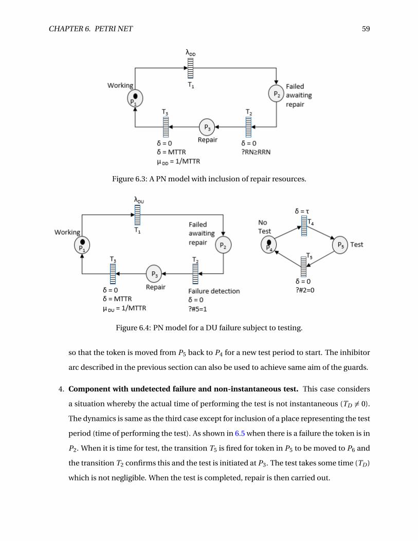
CHAPTER 6. PETRI NET 59
Figure 6.3: A PN model with inclusion of repair resources.
Figure 6.4: PN model for a DU failure subject to testing.
so that the token is moved from P5 back to P4 for a new test period to start. The inhibitor
arc described in the previous section can also be used to achieve same aim of the guards.
4. Component with undetected failure and non-instantaneous test. This case considers
a situation whereby the actual time of performing the test is not instantaneous (TD 6= 0).
The dynamics is same as the third case except for inclusion of a place representing the test
period (time of performing the test). As shown in 6.5 when there is a failure the token is in
P2. When it is time for test, the transition T5 is fired for token in P5 to be moved to P6 and
the transition T2 confirms this and the test is initiated at P3. The test takes some time (TD )
which is not negligible. When the test is completed, repair is then carried out.
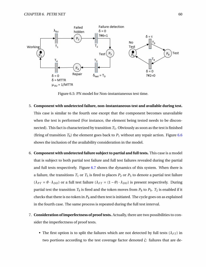
CHAPTER 6. PETRI NET 60
Figure 6.5: PN model for Non-instantaneous test time.
5. Component with undetected failure, non-instantaneous test and available during test.
This case is similar to the fourth one except that the component becomes unavailable
when the test is performed (For instance, the element being tested needs to be discon-
nected). This fact is characterized by transition T5. Obviously as soon as the test is finished
(firing of transition T6) the element goes back to P1 without any repair action. Figure 6.6
shows the inclusion of the availability consideration in the model.
6. Component with undetected failure subject to partial and full tests. This case is a model
that is subject to both partial test failure and full test failures revealed during the partial
and full tests respectively. Figure 6.7 shows the dynamics of this system. When there is
a failure, the transitions T1 or T5 is fired to places P2 or P5 to denote a partial test failure
(λPT = θ ·λDU ) or a full test failure (λF T = (1− θ) ·λDU ) is present respectively. During
partial test the transition T9 is fired and the token moves from P8 to P9. T2 is enabled if it
checks that there is no token in P8 and then test is initiated. The cycle goes on as explained
in the fourth case. The same process is repeated during the full test interval.
7. Consideration of imperfectness of proof tests. Actually, there are two possibilities to con-
sider the imperfectness of proof tests.
• The first option is to split the failures which are not detected by full tests (λF T ) in
two portions according to the test coverage factor denoted ξ: failures that are de-
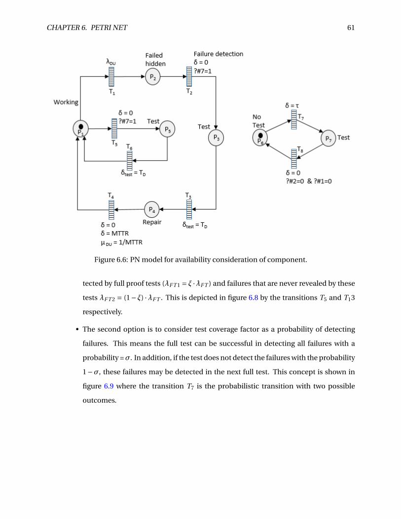
CHAPTER 6. PETRI NET 61
Figure 6.6: PN model for availability consideration of component.
tected by full proof tests (λF T 1 = ξ ·λF T ) and failures that are never revealed by these
tests λF T 2 = (1−ξ) ·λF T . This is depicted in figure 6.8 by the transitions T5 and T13
respectively.
• The second option is to consider test coverage factor as a probability of detecting
failures. This means the full test can be successful in detecting all failures with a
probability =σ. In addition, if the test does not detect the failures with the probability
1−σ, these failures may be detected in the next full test. This concept is shown in
figure 6.9 where the transition T7 is the probabilistic transition with two possible
outcomes.
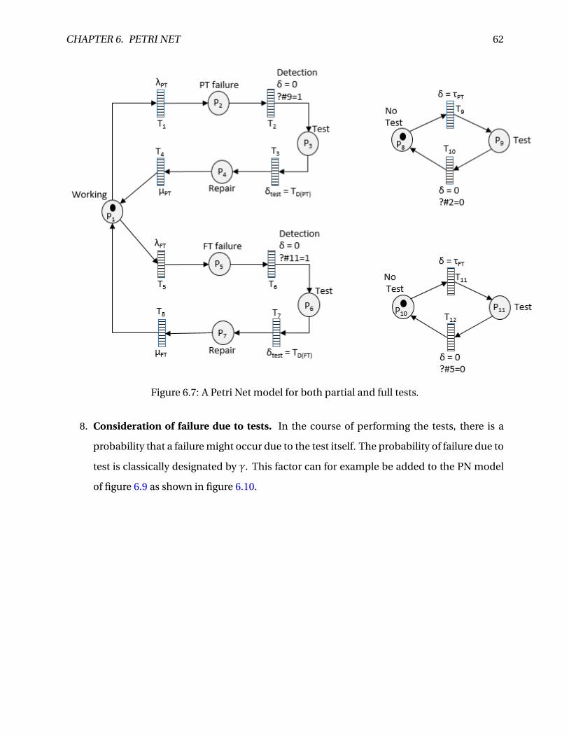
CHAPTER 6. PETRI NET 62
Figure 6.7: A Petri Net model for both partial and full tests.
8. Consideration of failure due to tests. In the course of performing the tests, there is a
probability that a failure might occur due to the test itself. The probability of failure due to
test is classically designated by γ. This factor can for example be added to the PN model
of figure 6.9 as shown in figure 6.10.
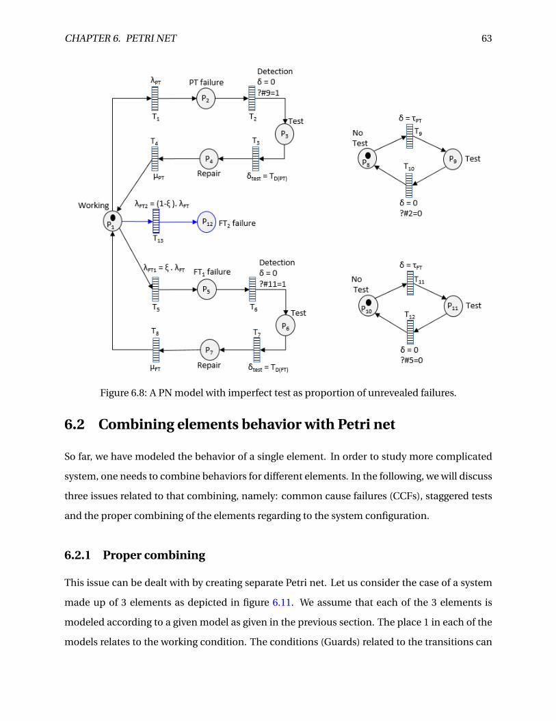
CHAPTER 6. PETRI NET 63
Figure 6.8: A PN model with imperfect test as proportion of unrevealed failures.
6.2 Combining elements behavior with Petri net
So far, we have modeled the behavior of a single element. In order to study more complicated
system, one needs to combine behaviors for different elements. In the following, we will discuss
three issues related to that combining, namely: common cause failures (CCFs), staggered tests
and the proper combining of the elements regarding to the system configuration.
6.2.1 Proper combining
This issue can be dealt with by creating separate Petri net. Let us consider the case of a system
made up of 3 elements as depicted in figure 6.11. We assume that each of the 3 elements is
modeled according to a given model as given in the previous section. The place 1 in each of the
models relates to the working condition. The conditions (Guards) related to the transitions can
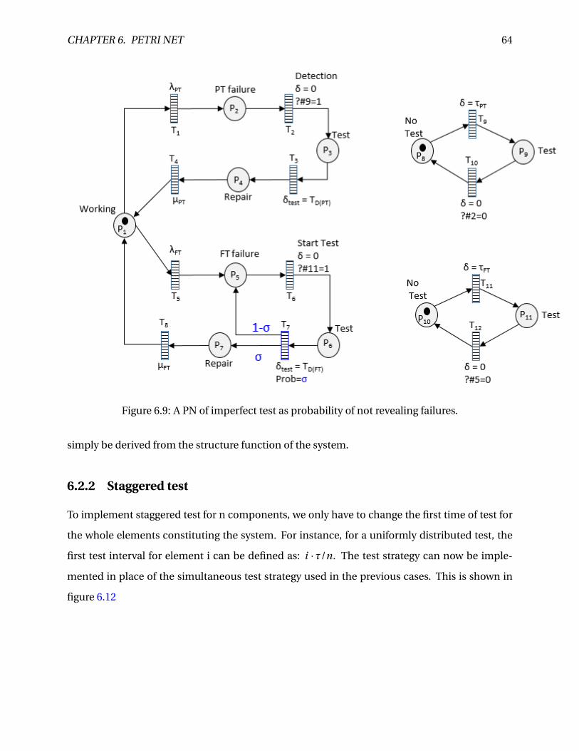
CHAPTER 6. PETRI NET 64
Figure 6.9: A PN of imperfect test as probability of not revealing failures.
simply be derived from the structure function of the system.
6.2.2 Staggered test
To implement staggered test for n components, we only have to change the first time of test for
the whole elements constituting the system. For instance, for a uniformly distributed test, the
first test interval for element i can be defined as: i ·τ/n. The test strategy can now be imple-
mented in place of the simultaneous test strategy used in the previous cases. This is shown in
figure 6.12
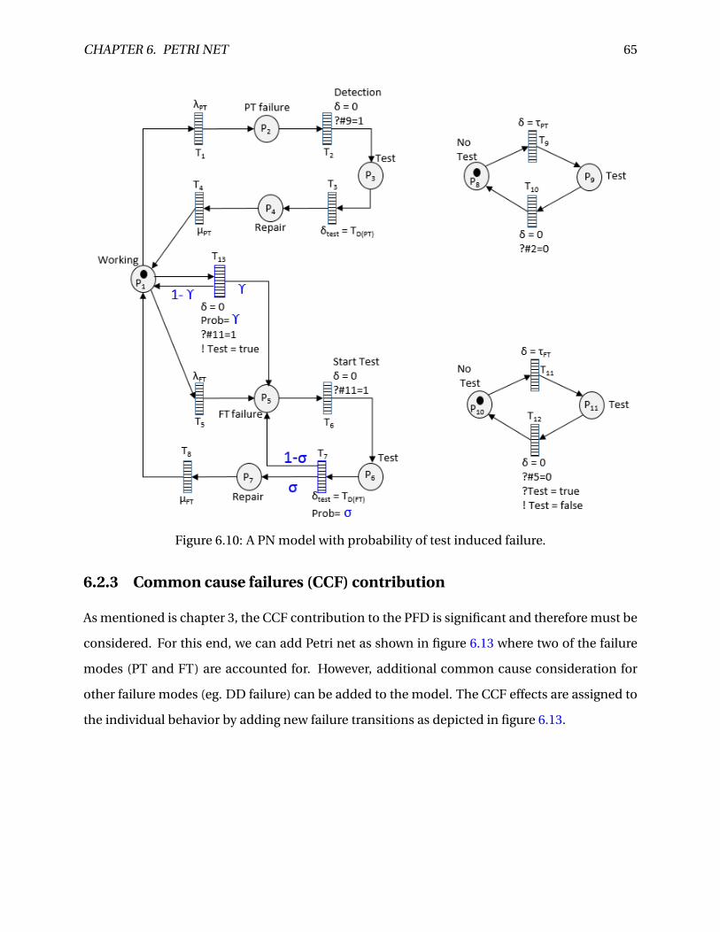
CHAPTER 6. PETRI NET 65
Figure 6.10: A PN model with probability of test induced failure.
6.2.3 Common cause failures (CCF) contribution
As mentioned is chapter 3, the CCF contribution to the PFD is significant and therefore must be
considered. For this end, we can add Petri net as shown in figure 6.13 where two of the failure
modes (PT and FT) are accounted for. However, additional common cause consideration for
other failure modes (eg. DD failure) can be added to the model. The CCF effects are assigned to
the individual behavior by adding new failure transitions as depicted in figure 6.13.
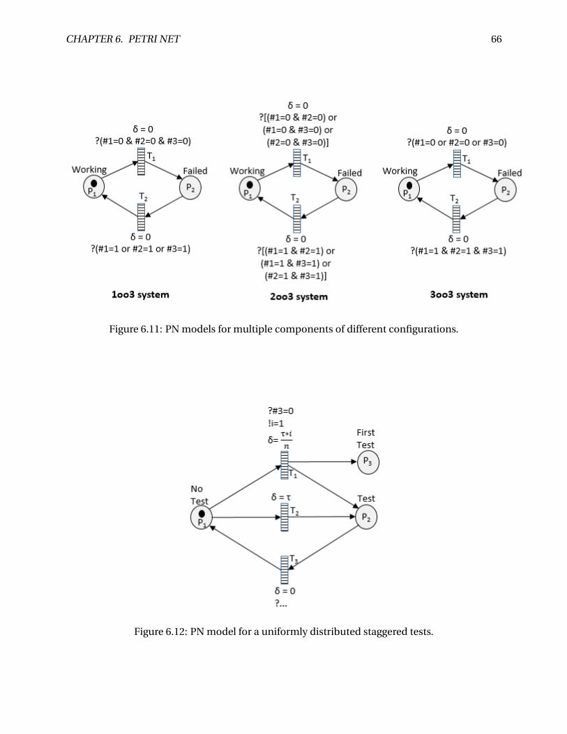
CHAPTER 6. PETRI NET 66
Figure 6.11: PN models for multiple components of different configurations.
Figure 6.12: PN model for a uniformly distributed staggered tests.
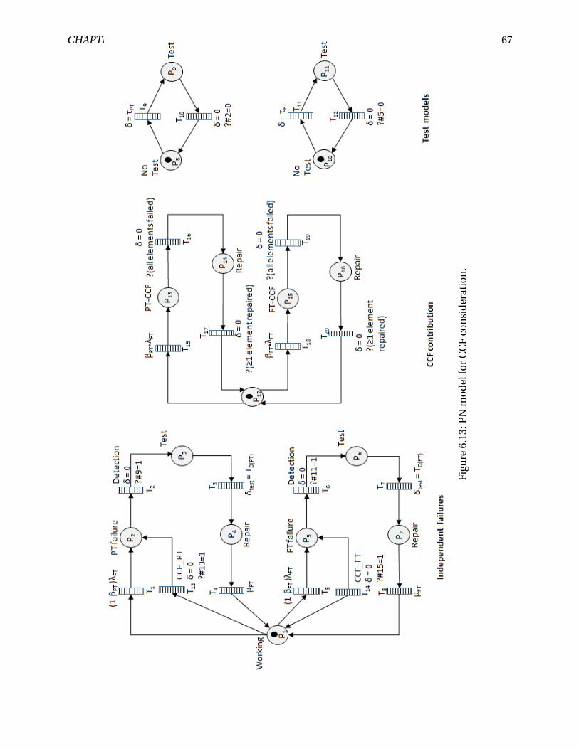
CHAPTER 6. PETRI NET 67
Fig
ure
6.13
:PN
mo
del
for
CC
Fco
nsi
der
atio
n.
Chapter 7
Case study
7.1 Chemical reactor protection system (CRPS)
This chapter presents the case study and uses the reliability assessment methods described in
the previous chapters to demonstrate the effect of partial and imperfect testing on the reliability
of a SIS.
7.1.1 System description
In this section, the case study described below taken from Torres-Echeverria et al. (2009) is used
to illustrate the use of fault tree driven multi-phase Markov and Petri nets approaches described
in the previous chapter. The case study is a protection system designed and implemented to
control high temperature and pressure of a chemical reactor. The system is composed of four
subsystems namely:Temperature transmitter (TT), pressure transmitter (PT), logic solver (LS)
and the final control element (FC). When high pressure or temperature is detected by the trans-
mitters, the system should shut the supply source to the reactor in order to prevent explosion
of reactor. The structure of the system is shown in figure 7.1 below. Each subsystem is parallel
redundant. The sensor layer is made up of two transmitters:Temperature transmitter (TT) and
pressure transmitter (PT), structured in 1oo2 architecture. The Logic Solver layer (LS) structured
in 1oo3 architecture and the final control (FC) layer is structured in 1oo3 architecture, made up
of three valves (Torres-Echeverria et al., 2009; Mechri et al., 2015). The reliability block diagram
68
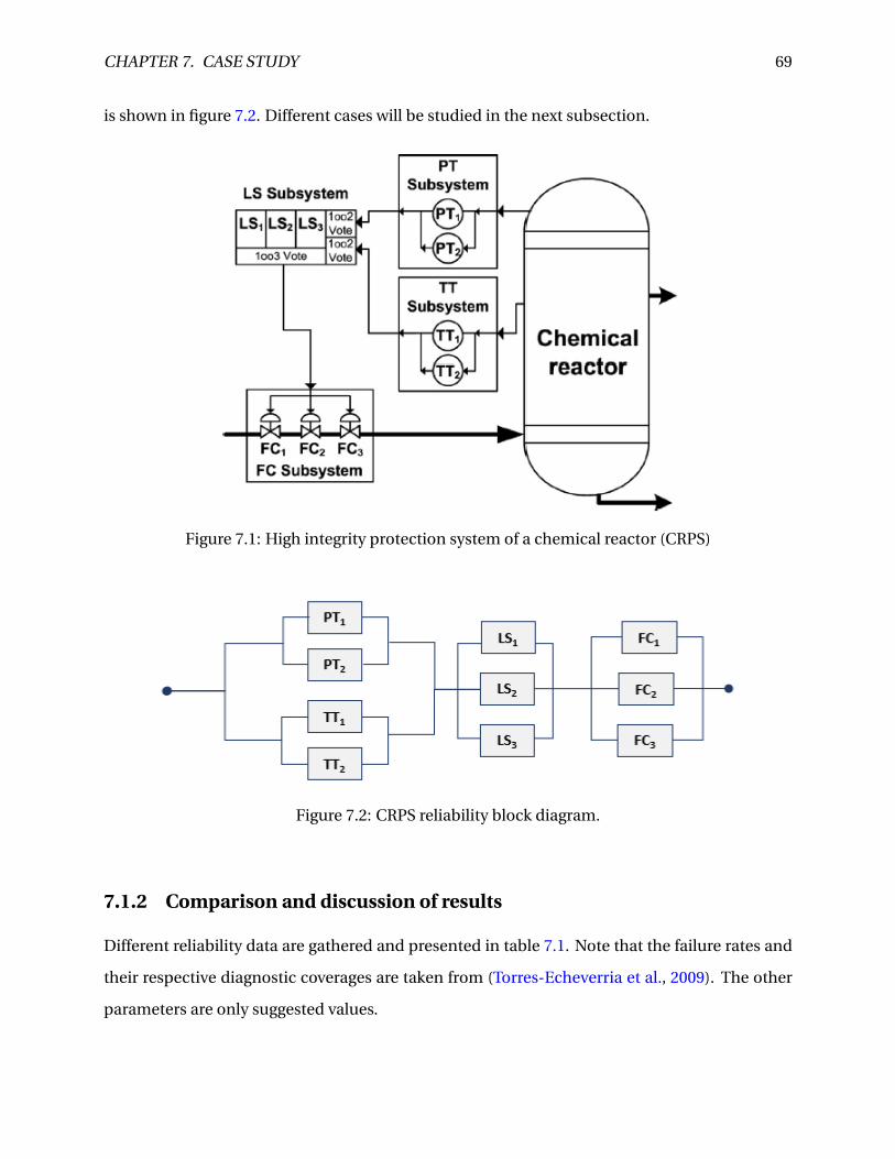
CHAPTER 7. CASE STUDY 69
is shown in figure 7.2. Different cases will be studied in the next subsection.
Figure 7.1: High integrity protection system of a chemical reactor (CRPS)
Figure 7.2: CRPS reliability block diagram.
7.1.2 Comparison and discussion of results
Different reliability data are gathered and presented in table 7.1. Note that the failure rates and
their respective diagnostic coverages are taken from (Torres-Echeverria et al., 2009). The other
parameters are only suggested values.

CHAPTER 7. CASE STUDY 70
Parameters LS (Safety PLC) PT (Electronic) TT (Switch) FC (Air operated valve)
λD (1E −6/h) 0.032 1.90 7.60 3.35DC (%) 81.25 51.1 10 25τ(h) 8760 4380 4380 4380MTTR=MRT (h) 8 8 8 8
Other parameters common to all components:β= 0.1 and βD = 0.05Proof test coverage ξ= 0.8Probability of detecting failure σ= 0.8
Table 7.1: Parameters for the system analysis
For formula comparison purposes where applicable (case 1 and case 2), the formula given
in Chebila and Innal (2015) is used and given in equation 7.1:
PF DK ooN ≈( n
n−k+1
)(n −k +2) ·λ(i )
DU ·m ·TST
·m−1∑j=0
[( λ(i )DD
λ(i )DD +µDD
+ (λ(i )
DU +λ(i )PT · j
) ·TST
)n−k+2
−( λ(i )
DD
λ(i )DD +µDD
+λ(i )PT · j ·TST
)n−k+2]+ λ(CC F )
DD
λ(CC F )DD +µDD
+λ(CC F )ST · TST
2+ λ(CC F )
PT · T1
2(7.1)
The fault tree and Petri net models are built in GRIF. CCFs are considered. The value 0.8 for
ξ was used both for the proportion and for the probability σ. The robust nature of the GRIF
software allowed for the consideration of staggered tests and uncertain parameters that follow
uniform distribution. The two options (1 and 2) mentioned in the cases mean:
• Option 1: The first option is to split the failures which are not detected by the full proof
tests (λF T ) in two portions according to the test coverage factor denoted ξ: failures that
are detected by full proof tests (λF T 1 = ξ·λF T ) and failures that are never revealed by these
tests λF T 2 = (1−ξ) ·λF T .
• Option 2: The second option is to consider test coverage factor as a probability of detect-
ing failures σ. This means the full test can be successful in detecting all failures with a
probability = σ. In addition, if the test does not detect the failures with the probability
1−σ, these failures may be detected in the next full test.
The FT-MPM and MC-PN in the table mean fault tree driven multi-phase Markov and Monte
Carlo Petri net respectively.
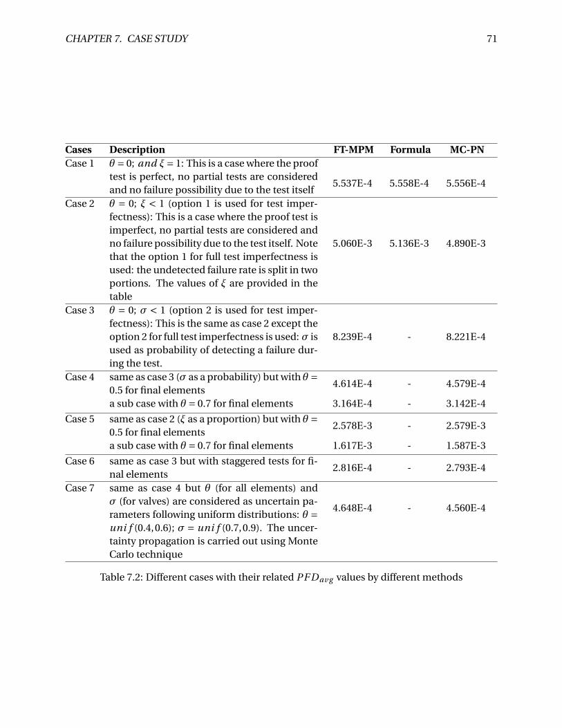
CHAPTER 7. CASE STUDY 71
Cases Description FT-MPM Formula MC-PNCase 1 θ = 0; and ξ= 1: This is a case where the proof
test is perfect, no partial tests are consideredand no failure possibility due to the test itself
5.537E-4 5.558E-4 5.556E-4
Case 2 θ = 0; ξ < 1 (option 1 is used for test imper-fectness): This is a case where the proof test isimperfect, no partial tests are considered andno failure possibility due to the test itself. Notethat the option 1 for full test imperfectness isused: the undetected failure rate is split in twoportions. The values of ξ are provided in thetable
5.060E-3 5.136E-3 4.890E-3
Case 3 θ = 0; σ < 1 (option 2 is used for test imper-fectness): This is the same as case 2 except theoption 2 for full test imperfectness is used: σ isused as probability of detecting a failure dur-ing the test.
8.239E-4 - 8.221E-4
Case 4 same as case 3 (σ as a probability) but with θ =0.5 for final elements
4.614E-4 - 4.579E-4
a sub case with θ = 0.7 for final elements 3.164E-4 - 3.142E-4
Case 5 same as case 2 (ξ as a proportion) but with θ =0.5 for final elements
2.578E-3 - 2.579E-3
a sub case with θ = 0.7 for final elements 1.617E-3 - 1.587E-3
Case 6 same as case 3 but with staggered tests for fi-nal elements
2.816E-4 - 2.793E-4
Case 7 same as case 4 but θ (for all elements) andσ (for valves) are considered as uncertain pa-rameters following uniform distributions: θ =uni f (0.4,0.6); σ = uni f (0.7,0.9). The uncer-tainty propagation is carried out using MonteCarlo technique
4.648E-4 - 4.560E-4
Table 7.2: Different cases with their related PF Dav g values by different methods
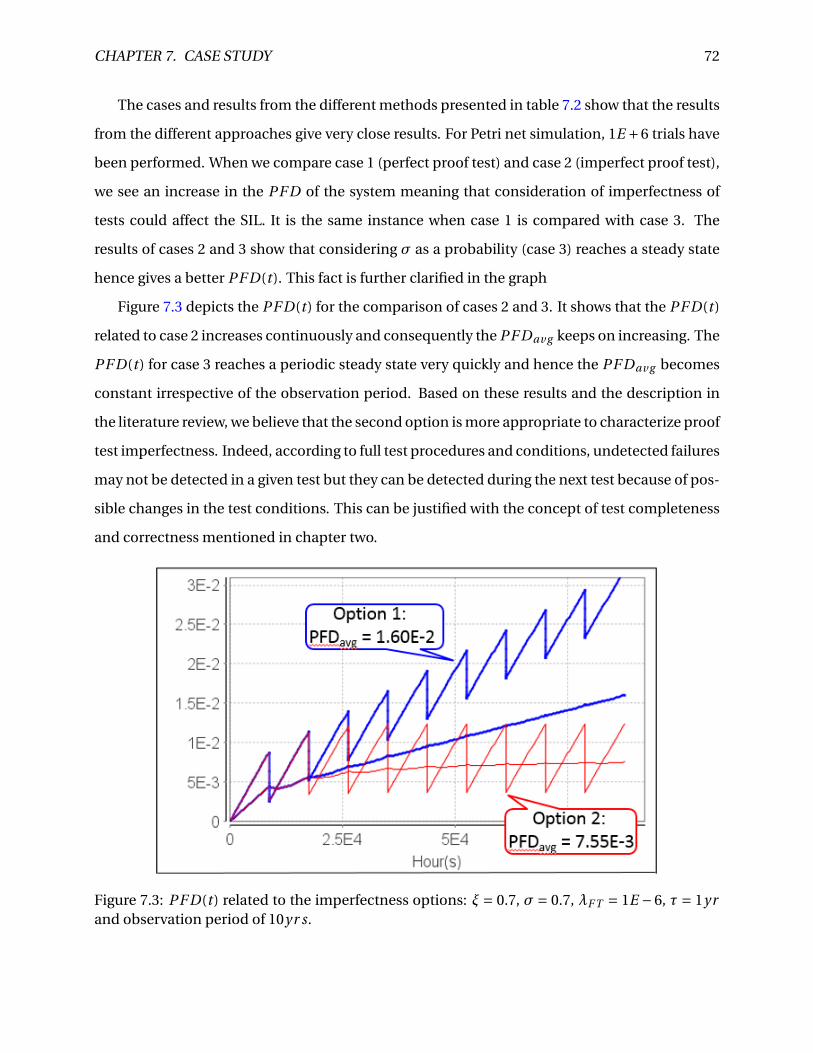
CHAPTER 7. CASE STUDY 72
The cases and results from the different methods presented in table 7.2 show that the results
from the different approaches give very close results. For Petri net simulation, 1E +6 trials have
been performed. When we compare case 1 (perfect proof test) and case 2 (imperfect proof test),
we see an increase in the PF D of the system meaning that consideration of imperfectness of
tests could affect the SIL. It is the same instance when case 1 is compared with case 3. The
results of cases 2 and 3 show that considering σ as a probability (case 3) reaches a steady state
hence gives a better PF D(t ). This fact is further clarified in the graph
Figure 7.3 depicts the PF D(t ) for the comparison of cases 2 and 3. It shows that the PF D(t )
related to case 2 increases continuously and consequently the PF Dav g keeps on increasing. The
PF D(t ) for case 3 reaches a periodic steady state very quickly and hence the PF Dav g becomes
constant irrespective of the observation period. Based on these results and the description in
the literature review, we believe that the second option is more appropriate to characterize proof
test imperfectness. Indeed, according to full test procedures and conditions, undetected failures
may not be detected in a given test but they can be detected during the next test because of pos-
sible changes in the test conditions. This can be justified with the concept of test completeness
and correctness mentioned in chapter two.
Figure 7.3: PF D(t ) related to the imperfectness options: ξ = 0.7, σ = 0.7, λF T = 1E −6, τ = 1yrand observation period of 10yr s.
CHAPTER 7. CASE STUDY 73
Case 4 includes implementation of partial testing in addition to case 3 and we can see the
reduction in the PF Dav g . Note that the partial test introduced is only on the final elements
but still showed a reasonable decrease in the PF D(t ) when compared with the results in case
3. An increase of the partial test coverage factor θ shows a further decrease in the PF Dav g .
This emphasizes the importance of determining accurate test coverages. Case 5 is similar to
case 4 but here, the partial test coverage is introduced with the option of ξ as a proportion of
unrevealed failures. When this case is compared to case 2, we also see a decrease in the result
by the introduction of partial test and a further decrease by an increase the partial test coverage
factor θ. The partial test interval used for these cases is 1 month (730 hours). It is worth noting
that in case 5, even with θ = 0.7, the corresponding PF Dav g is still higher compared to cases 3
(θ = 0) and 4 (θ = 0.5 & 0.7). This shows that option 1 for test imperfectness is very pessimistic
compared to the option 2. Note that for this case, there is no available analytical formula in the
literature except for a 1oo1 system (Rolén, 2007).
In case 6, a staggered test strategy is implemented. This was done by changing the time of
first test as explained with the Petri net model in the previous chapter. When we compare this
case with case 3, the results show a decrease meaning that staggered tests have positive impact
on the PF Dav g of the system. This justifies the fact that staggered tests reduces the possibility of
CCFs mentioned in chapter 2. However, there might be some disadvantages with implementing
staggered tests like extra costs and resources that may be involved.
The last case which considers the θ and σ as uncertain parameters following a uniform dis-
tribution gives results close to case 4. When uncertainties are considered, we can have lower
results as in the case of the fault tree approach of case 7 compared with case 4 with θ = 0.5. This
is however not the case with the PN result. The reason may be the number of iterations carried
out. 10000 iterations was used for the fault tree and only 1000 for the Petri net due to simula-
tion time. Other correct distributions for any parameters could be used like the lognormal. The
graph in figure 7.4 shows the propagation of the result with the upper and lower boundaries.
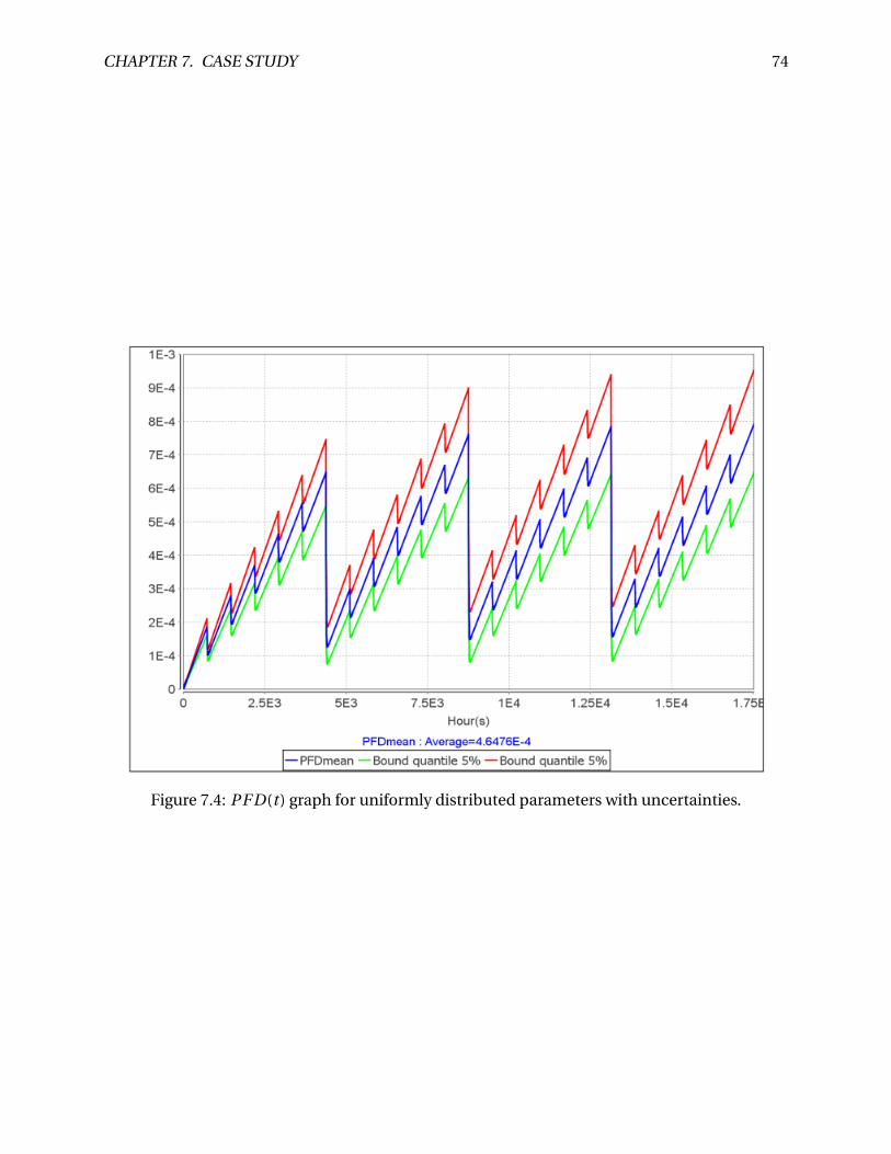
CHAPTER 7. CASE STUDY 74
Figure 7.4: PF D(t ) graph for uniformly distributed parameters with uncertainties.
Chapter 8
Discussion and Conclusion
8.1 Discussion
In performing reliability assessments, many assumptions are made as regards the system being
analyzed and the conditions in which they operate. Results from the assessments influence the
design of a SIS to a large extent therefore, care should be taken to incorporate the assumptions
and uncertainties into the assessment, so that results are not misinterpreted.
In this thesis, we looked at three approaches to consider imperfectness of tests. First is the
IEC 61508 approach where the proof test coverage (PTC) is considered as a proportion (fraction)
of DU failures that are revealed by the proof test. This is also represented by the Greek letter
ξ. Secondly, we analysed imperfectness as the probability of detecting a DU failure during a
given proof test. The Greek alphabet σ was used to denote this probability. The third approach
considered is the PDS method which introduces the addition of a constant (probability of test
independent failures (PT I F )) for modeling the effect of imperfect proof tests due to systematic
failures.
Furthermore, different methods of performing reliability assessments were used. We looked
at the use of analytical formulas. The cases analyzed in chapter seven reveals there are some
complicated cases where analytical formulas are not available. In chapter five, we used the
multi-phase Markov approach and discussed the limitation regarding states explosion with com-
plex models (e.g. higher configuration) and other failure considerations. This thesis showed that
the fault tree approach whereby some basic events could be modelled using multi-phase Markov
75
CHAPTER 8. DISCUSSION AND CONCLUSION 76
(hence called fault tree driven multi-phase Markov) is a better approach compared to the two
earlier stated approaches. The flexibility and dynamism of the Petri net is shown in chapter six.
Here, different cases of how a PN model can be used were given. The case study is not a com-
plex one hence did not demonstrate how the PN approach is further used in complicated cases
where other methods are not feasible.
8.2 Conclusion
Having analyzed two options of considering the proof test coverage: as a proportion (fraction)
of DU failures that are revealed by the proof test ξ (the test does not cover all possible failures:
inadequate test method) and as a probability of detecting a DU failure during a given proof testσ
(test does not detect all the failures: unsuccessful test), we have shown that the use of the latter
is more appropriate. This is because undetected failures which are detected in a given proof
test may be detected during the next test because of possible changes in the test procedures
and conditions. The justifies the concept of test completeness and correctness described in
chapter two. The graph illustrating this fact is shown in chapter seven, figure 7.3. It is worth
noting that from the cases presented in table 7.2 in chapter seven, case 5 even with θ = 0.7,
the corresponding PF Dav g is still higher compared to cases 3 (θ = 0) and 4 (θ = 0.5&0.7). This
shows that option 1 for test imperfectness is very pessimistic compared to the option 2 therefore
validates our point that option 2 is more suitable. Note however that there may be cases where
a combination of two of the approaches may be more suitable.
When considering different complicated maintenance strategies (e.g. repair strategies and
resource availability) and system reconfiguration following a failure, only simulation will be the
suitable approach. This is to enable these factors to be considered in the modeling of the system
failure probability. A typical example of this is a degradation with repair process due to partial
tests. This can not be calculated except simulated using Petri net. Some of the cases in table 7.2
in chapter seven prove this fact.
This thesis has made it obvious that it is important to critically appraise and evaluate the
assumptions made when performing reliability calculations. The case of imperfectness of tests
justifies that disregarding the estimation of non-testable (non-detectable) failures could lead to

CHAPTER 8. DISCUSSION AND CONCLUSION 77
an inaccurate PFD result. With the increase in the use of SIS for risk reduction, improvement in
the quality of the reliability calculations is important.
8.3 Recommendations for further work
In the course of this master’s thesis, some interesting aspects of partial and imperfect testing
which more clarification and better understanding are needed were unveiled.
• The procedures for determination of the partial stroke test coverage factor θ suggested
in Lundteigen and Rausand (2008a) needs to be generalized to be applicable to different
equipment.
• Adequate procedures for finding a realistic value of the full proof test coverage factor ξ or
PTC as proportion of non-testable or non-detectable failures should be researched. In a
case where the probabilistic value is considered, the appropriate probability value needs
to be determined.
• There are some case cases where the partial tests results in degradation of components.
An example is a case of a ball valve being partial tested by rotating to say 20 %, which
could cause wear and building up of sediments which may affect the full closing of the
valve. How can this degradation factor be considered in partial test calculation?

Bibliography
Aguilar Martinez, W. A. (2014). Methods for determining pfd/sil for workover control systems
with short test-intervals and imperfect testing.
Ali, R., Goble, W., and Business, F. (2004). Smart positioners to predict health of esd valves. In AN-
NUAL SYMPOSIUM ON INSTRUMENTATION FOR THE PROCESS INDUSTRIES, volume 59,
pages 29–38. INSTRUMENT SOCIETY OF AMERICA.
Brissaud, F., Barros, A., and Bérenguer, C. (2012). Probability of failure on demand of safety
systems: impact of partial test distribution. Proceedings of the Institution of Mechanical Engi-
neers, Part O: Journal of Risk and Reliability, page 1748006X12448142.
Bukowski, J. V. and Van Beurden, I. (2009). Impact of proof test effectiveness on safety instru-
mented system performance. In Reliability and Maintainability Symposium, 2009. RAMS
2009. Annual, pages 157–163. IEEE.
Cepin, M. (1995). Sequential versus staggered testing towards dynamic psa.
Chebila, M. and Innal, F. (2015). Generalized analytical expressions for safety instrumented
systems’ performance measures: Pfd avg and pfh. Journal of Loss Prevention in the Process
Industries, 34:167–176.
David, R. and Alla, H. (2010). Discrete, continuous, and hybrid Petri nets. Springer Science &
Business Media.
Dutuit, Y., Innal, F., Rauzy, A., and Signoret, J.-P. (2008). Probabilistic assessments in relation-
ship with safety integrity levels by using fault trees. Reliability Engineering & System Safety,
93(12):1867–1876.
78
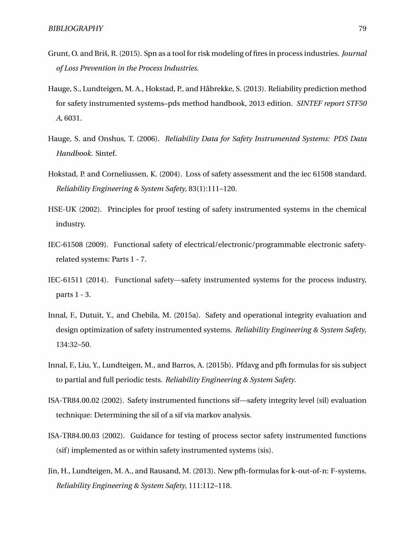
BIBLIOGRAPHY 79
Grunt, O. and Briš, R. (2015). Spn as a tool for risk modeling of fires in process industries. Journal
of Loss Prevention in the Process Industries.
Hauge, S., Lundteigen, M. A., Hokstad, P., and Håbrekke, S. (2013). Reliability prediction method
for safety instrumented systems–pds method handbook, 2013 edition. SINTEF report STF50
A, 6031.
Hauge, S. and Onshus, T. (2006). Reliability Data for Safety Instrumented Systems: PDS Data
Handbook. Sintef.
Hokstad, P. and Corneliussen, K. (2004). Loss of safety assessment and the iec 61508 standard.
Reliability Engineering & System Safety, 83(1):111–120.
HSE-UK (2002). Principles for proof testing of safety instrumented systems in the chemical
industry.
IEC-61508 (2009). Functional safety of electrical/electronic/programmable electronic safety-
related systems: Parts 1 - 7.
IEC-61511 (2014). Functional safety—safety instrumented systems for the process industry,
parts 1 - 3.
Innal, F., Dutuit, Y., and Chebila, M. (2015a). Safety and operational integrity evaluation and
design optimization of safety instrumented systems. Reliability Engineering & System Safety,
134:32–50.
Innal, F., Liu, Y., Lundteigen, M., and Barros, A. (2015b). Pfdavg and pfh formulas for sis subject
to partial and full periodic tests. Reliability Engineering & System Safety.
ISA-TR84.00.02 (2002). Safety instrumented functions sif—safety integrity level (sil) evaluation
technique: Determining the sil of a sif via markov analysis.
ISA-TR84.00.03 (2002). Guidance for testing of process sector safety instrumented functions
(sif) implemented as or within safety instrumented systems (sis).
Jin, H., Lundteigen, M. A., and Rausand, M. (2013). New pfh-formulas for k-out-of-n: F-systems.
Reliability Engineering & System Safety, 111:112–118.
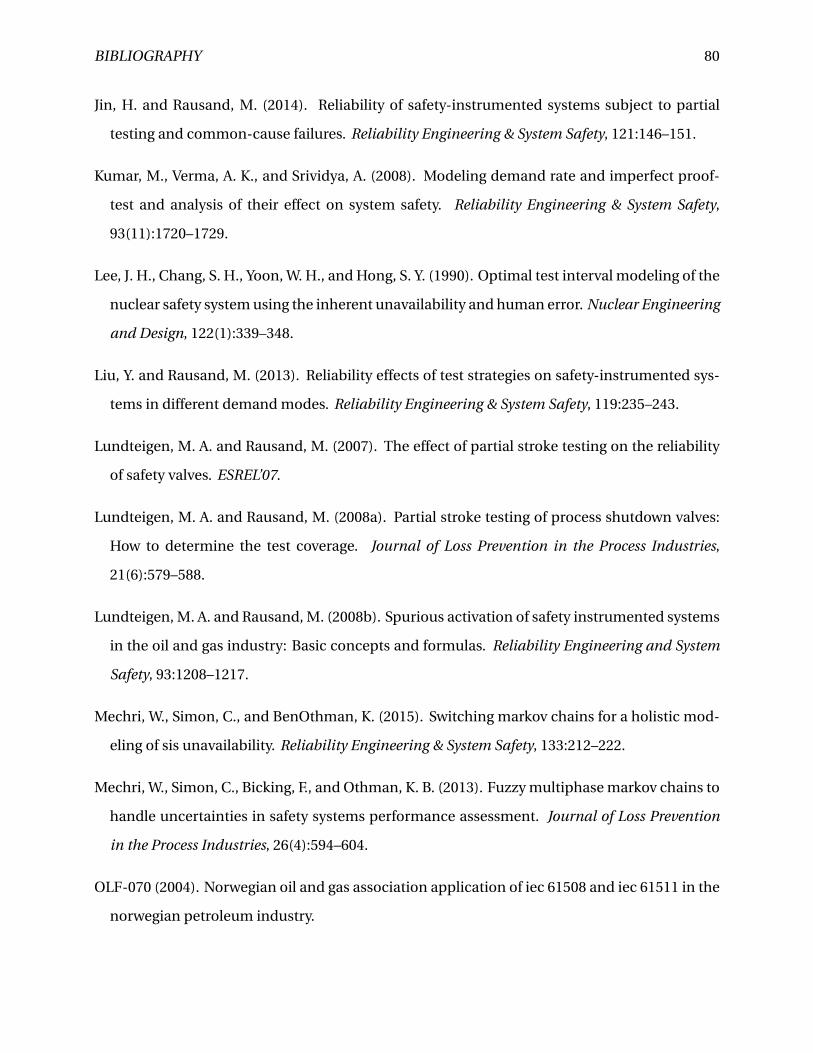
BIBLIOGRAPHY 80
Jin, H. and Rausand, M. (2014). Reliability of safety-instrumented systems subject to partial
testing and common-cause failures. Reliability Engineering & System Safety, 121:146–151.
Kumar, M., Verma, A. K., and Srividya, A. (2008). Modeling demand rate and imperfect proof-
test and analysis of their effect on system safety. Reliability Engineering & System Safety,
93(11):1720–1729.
Lee, J. H., Chang, S. H., Yoon, W. H., and Hong, S. Y. (1990). Optimal test interval modeling of the
nuclear safety system using the inherent unavailability and human error. Nuclear Engineering
and Design, 122(1):339–348.
Liu, Y. and Rausand, M. (2013). Reliability effects of test strategies on safety-instrumented sys-
tems in different demand modes. Reliability Engineering & System Safety, 119:235–243.
Lundteigen, M. A. and Rausand, M. (2007). The effect of partial stroke testing on the reliability
of safety valves. ESREL’07.
Lundteigen, M. A. and Rausand, M. (2008a). Partial stroke testing of process shutdown valves:
How to determine the test coverage. Journal of Loss Prevention in the Process Industries,
21(6):579–588.
Lundteigen, M. A. and Rausand, M. (2008b). Spurious activation of safety instrumented systems
in the oil and gas industry: Basic concepts and formulas. Reliability Engineering and System
Safety, 93:1208–1217.
Mechri, W., Simon, C., and BenOthman, K. (2015). Switching markov chains for a holistic mod-
eling of sis unavailability. Reliability Engineering & System Safety, 133:212–222.
Mechri, W., Simon, C., Bicking, F., and Othman, K. B. (2013). Fuzzy multiphase markov chains to
handle uncertainties in safety systems performance assessment. Journal of Loss Prevention
in the Process Industries, 26(4):594–604.
OLF-070 (2004). Norwegian oil and gas association application of iec 61508 and iec 61511 in the
norwegian petroleum industry.
BIBLIOGRAPHY 81
Oliveira, L. F. (2009). Pfd of higher-order configurations of sis with partial stroke testing capabil-
ity. pages 1919–1928.
Oliveira, L. F. and Abramovitch, R. N. (2010). Extension of isa tr84. 00.02 pfd equations to koon
architectures. Reliability Engineering & System Safety, 95(7):707–715.
Rausand, M. (2014). Reiability of Safety-Critical Systems: Theory and Applications. Wiley, Hobo-
ken, NJ.
Rausand, M. and Høyland, A. (2004). System Reliability Theory: Models, Statistical Methods, and
Applications. Wiley, Hoboken, NJ, 2nd edition.
Rauzy, A. (2008). Binary decision diagrams for reliability studies. In Handbook of Performability
Engineering, pages 381–396. Springer.
Rolén, H. (2007). Partial and imperfect testing of safety instrumented functions. PhD thesis,
Master thesis at NTNU.
Signoret, J.-P., Dutuit, Y., Cacheux, P.-J., Folleau, C., Collas, S., and Thomas, P. (2013). Make your
petri nets understandable: Reliability block diagrams driven petri nets. Reliability Engineer-
ing & System Safety, 113:61–75.
Summers, A. and Zachary, B. (2000). Partial-stroke testing of safety block valves. Control Engi-
neering, 47(12):87–89.
Torres-Echeverria, A., Martorell, S., and Thompson, H. (2009). Modelling and optimization of
proof testing policies for safety instrumented systems. Reliability Engineering & System Safety,
94(4):838–854.
Torres-Echeverria, A. C. (2009). Modelling and optimization of safety instrumented systems
based on dependability and cost measures.
Zhang, T., Wang, Y., and Xie, M. (2008). Analysis of the performance of safety-critical systems
with diagnosis and periodic inspection. In Reliability and Maintainability Symposium, 2008.
RAMS 2008. Annual, pages 143–148. IEEE.
Appendix A
Acronyms
CCF Common cause failure
DC Diagnostic coverage
EUC Equipment under control
FTA Fault tree analysis
MRT Mean restoration time
MTTR Mean time to repair
PFD Probability of failure on demand
PTC Proof test coverage
RBD Reliability block diagram
SIL Safety integrity level
SIS Safety instrumented system
SRS Safety requirement specification
82
Appendix B
Fault tree of the case study
The fault tree of the case study is a big one therefore has been divided into sub groups. The
group shown here is for final control element (FC). The fault tree for the independent and CCFs
for the other components (PT, TT and LS) are modeled the same way as the FC except that no
partial tests are considered.
B.1 General part of the fault tree of the case study
This fault tree is shown in figure B.1
B.2 Fault tree for independent failures of the FC
This fault tree is shown in figure B.2
B.3 Fault tree of CCF for the final control (FC) element
This fault tree is shown in figure B.3
83
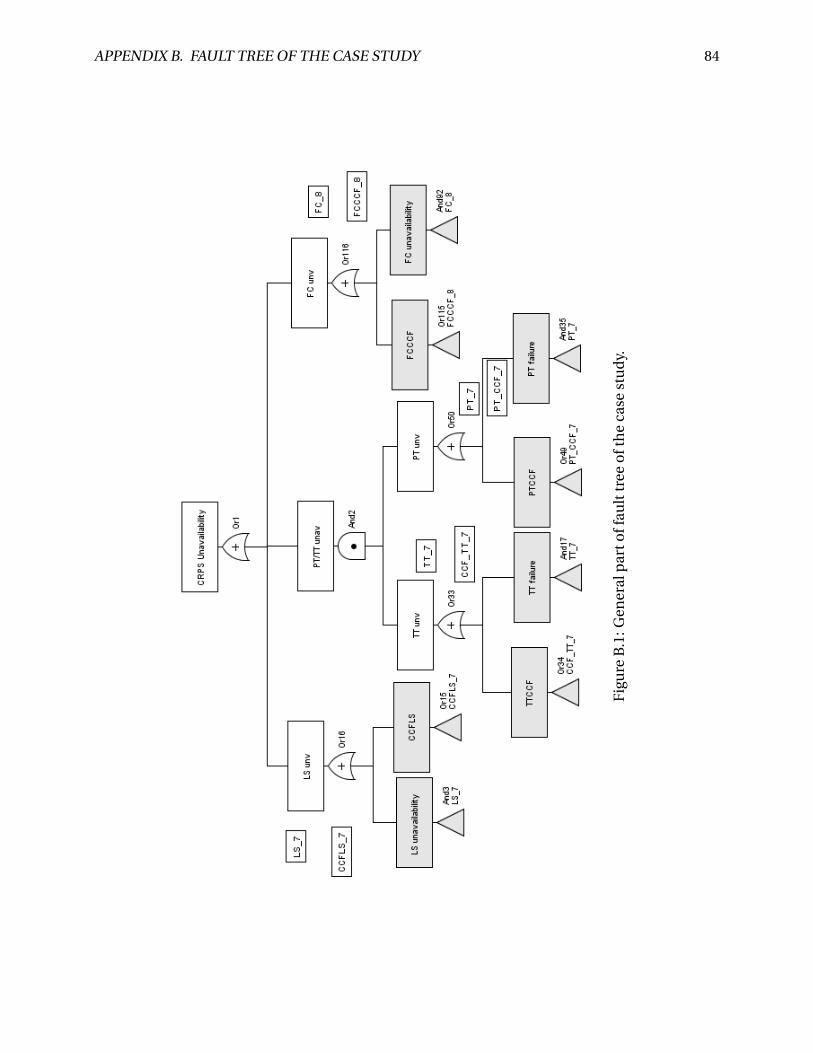
APPENDIX B. FAULT TREE OF THE CASE STUDY 84
Fig
ure
B.1
:Gen
eral
par
toff
ault
tree
oft
he
case
stu
dy.
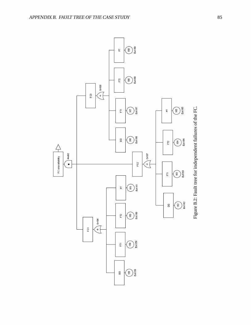
APPENDIX B. FAULT TREE OF THE CASE STUDY 85
Fig
ure
B.2
:Fau
lttr
eefo
rin
dep
end
entf
ailu
res
oft
he
FC
.
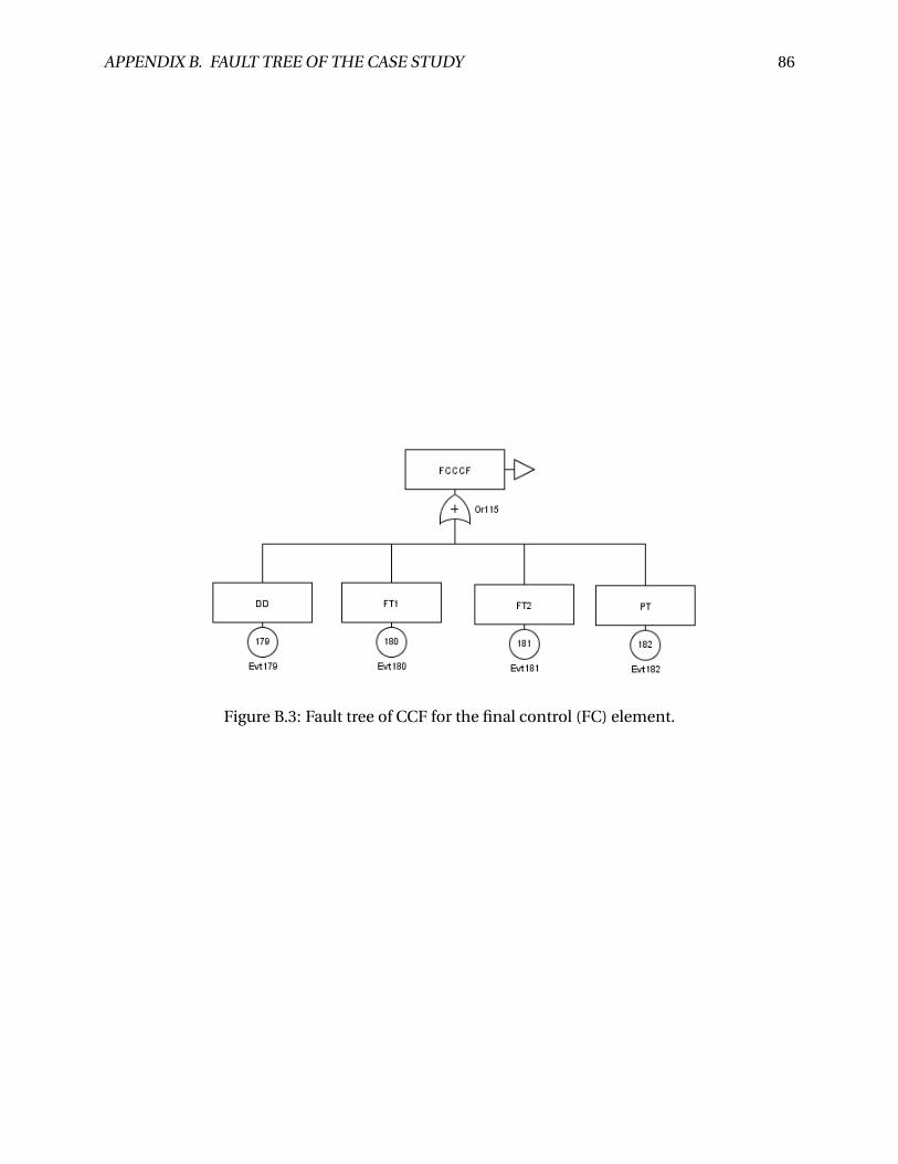
APPENDIX B. FAULT TREE OF THE CASE STUDY 86
Figure B.3: Fault tree of CCF for the final control (FC) element.
Appendix C
Petri net model of the case study
The Petri net model of the case study was designed and simulated using the GRIF software.
The picture in C.1 shows the representation for only two components (considering DD, FT1,
FT2 failures), the test model and the common cause model. Note that this is only page 1 of 12
pages of the complete model. PT failure is further considered when modelling the final control
elements.
87
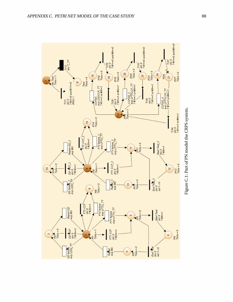
APPENDIX C. PETRI NET MODEL OF THE CASE STUDY 88
Fig
ure
C.1
:Par
tofP
Nm
od
elth
eC
RP
Ssy
stem
.
Appendix D
The use of MAPLE software
A sample of the use of MAPLE for formula generation for different configuration is shown here.
This is also used for calculations where necessary. Figure D.1 shows the Oliveira’s formula gen-
eration code used in chapter 3. Similar codes have been used for formulas of different authors.
89
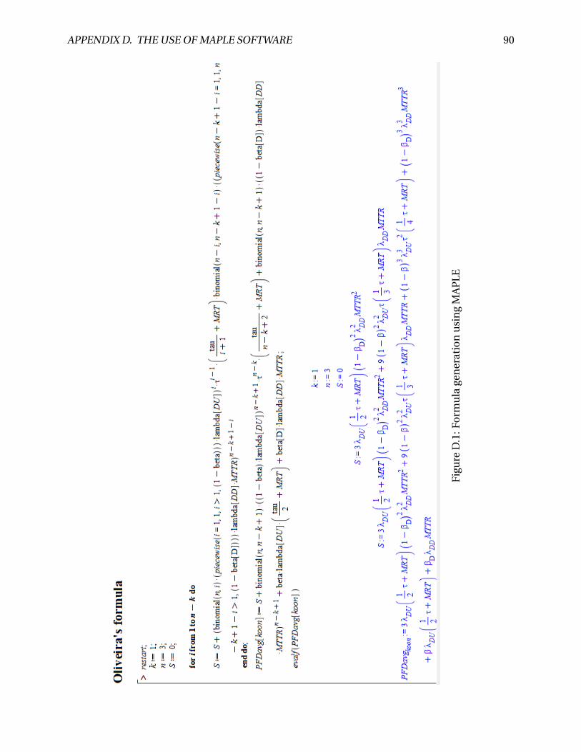
APPENDIX D. THE USE OF MAPLE SOFTWARE 90
Fig
ure
D.1
:Fo
rmu
lage
ner
atio
nu
sin
gM
AP
LE