Impact of PCTs on Demand Response - Phase II · Impact of PCTs on Demand Response – Phase II ACKNOWLEDGEMENTS Southern California Edison’s Design & Engineering Services (D&ES)

IMPACT OF PCTS ON DEMAND RESPONSE – PHASE II Analysis of the Demand Response of Commercial and Multifamily Residential HVAC Systems using Programmable Communicating Thermostats

DR 06.10 Draft Report

Prepared by:

Design & Engineering Services Customer Service Business Unit Southern California Edison

April 2007

Impact of PCTs on Demand Response – Phase II

ACKNOWLEDGEMENTS Southern California Edison’s Design & Engineering Services (D&ES) group is responsible for this project in collaboration with Tariff & Program Services (TP&S). It was developed as part of Southern California Edison’s Demand Response, Emerging Markets and Technologies program under internal project number DR 06.10. James J. Hirsch & Associates was the primary subcontractor on this project with overall management by Carlos Haiad of D&ES and Lauren Pemberton of TP&S. For more information on this project, email [email protected].

DISCLAIMER This report was prepared by Southern California Edison (SCE) and funded by California utility customers under the auspices of the California Public Utilities Commission. Reproduction or distribution of the whole or any part of the contents of this document without the express written permission of SCE is prohibited. This work was performed with reasonable care and in accordance with professional standards. However, neither SCE nor any entity performing the work pursuant to SCE’s authority make any warranty or representation, expressed or implied, with regard to this report, the merchantability or fitness for a particular purpose of the results of the work, or any analyses, or conclusions contained in this report. The results reflected in the work are generally representative of operating conditions; however, the results in any other situation may vary depending upon particular operating conditions.

Southern California Edison Design & Engineering Services April 2007

Abbreviations and Acronyms

ABBREVIATIONS AND ACRONYMS PCT Programmable Communicating Thermostat

RTU Rooftop (HVAC) Unit

EIR Energy Input Ratio (energy input divided by useful energy output)

ODB Outside Dry-bulb temperature, oF

EWB Coil Entering Wet-bulb temperature, oF

HVAC Heating, Ventilating and Air-Conditioning system


Executive Summary

EXECUTIVE SUMMARY This project analyzes the potential electricity demand response of small commercial HVAC systems and residential split air-conditioners due to the use of programmable communicating thermostats (PCTs). Phase I of this project looked at three of the most common applications: small office buildings, small retail buildings and single-family residential buildings. This phase (Phase II) of the project expands the original analysis with the addition of seventeen additional building types.

New HVAC performance curves were developed for rooftop packaged HVAC systems in the range of 5 – 10 tons. A range of dual compressor 10-ton units and single-compressor 5-ton units were derived from currently available equipment from the major manufacturers. These performance curves were utilized in the latest version of DOE2.2, a detailed hourly building simulation program.

Over 70,000 simulations were conducted using DOE2.2 to capture the range of building types, climate zones, HVAC configurations and control periods being considered. Each of these simulations model multiple HVAC systems within the building and in all, more than 750,000 sets of demand impacts were calculated.

A spreadsheet tool is provided that allows a user to filter the large database of results down to the specific building types, climate zones, building configurations and control periods of interest. Graphics provide a quick overview of the filtered data and tables provide the basis for further third-party utilization of the results.

Two aspects that affect the demand savings and that were beyond the scope of Phase I of this project were investigated in this report. Six sets of HVAC performance curves that represent the variety of potential HVAC systems currently in use were utilized to determine the range of demand impacts that can be expected from the use of PCTs in one building type and in a range of climate zones. The choice of a particular HVAC unit is shown to impact the demand response by approximately ±15%.

Staged-volume rooftop HVAC systems, such as the one currently being tested by SCE, offer the potential for greater demand savings impact by being able to lower the supply airflow setting as well as decreasing compressor use during control periods. Analysis conducted for this project shows the potential for 10 – 30% increased demand savings over constant volume systems due to the use of staged volume systems.


Introduction

INTRODUCTION This project analyzes the potential electricity demand response of small commercial HVAC systems and residential split air-conditioners due to the use of programmable communicating thermostats (PCTs). Phase I of this project looked at three of the most common applications: small office buildings, small retail buildings and single-family residential buildings. Phase II of the project expands the original analysis with the addition of seventeen additional building types.

For these new building types, a range of building shells and HVAC configurations are examined for the sixteen standard California climate zones. The combination of shell and HVAC options used are intended to capture the range of cooling loads that will be encountered during a given demand period.

Twenty-one thermostat control periods, defined by a starting hour and duration, are applied to each of the building/HVAC combinations for both the hottest day and tenth hottest day of each climate zone. All of these options lead to a total of more than 750,000 individual results derived from more than 70,000 simulations. Due to the vast data set generated by this project, significant effort was required to distill the data down to a smaller number of weighted data sets that can be reviewed and utilized by program planners.

THE BUILDING TYPES All of the building prototypes used in the energy simulations were derived from the 2005 DEER Update Project. Shell characteristics, internal gains and operating schedules were taken directly from the study. Some of the buildings geometries were modified from the DEER definitions to improve the solar neutrality or to better match the building types being targeted. Any deviations from the 2005 DEER prototypes are noted below.

Typically, the number of zones PCT-controlled with the PCT is equivalent to the total number of zones in the model. However, in some cases, not all zones are under PCT control. Guest rooms in the hotel, living quarters in the nursing home and laboratory areas in the bio/tech manufacturing building are some examples.

For some of the larger building models, such as the university, a subset of all the PCT-controlled zones are tracked for the demand analysis. The tracked zones in these buildings are chosen to capture the potential diversity of space loads while eliminating redundant results (i.e. identical spaces). In these cases, each of the tracked zones is weighted so that the sum of the weighted results represents the whole building.

Southern California Edison Page 2 Design & Engineering Services April 2007

Introduction

TABLE 1. BUILDING TYPES INCLUDE IN THIS STUDY

BUILDING TYPE

NUMBER OF ZONES

PCT-CONTROLLED (TRACKED)

TOTAL PCT-CONTROLLED AREA

(FT2)

Assembly 5 34,000

Education - Primary 14 50,000

Education – Secondary (High School) 49 (25) 150,000

Education - College 47 (23) 300,000

Education - University 61 (25) 1,000,000

Education – Relocatable Classroom 2 1922

Grocery 3 46,357

Nursing Home 18 33,326

Hotel 16 53,245

Motel 1 2000

Manufacturing – Light Industrial 3 100,000

Manufacturing – Bio/Technology 8 65,315

Restaurant - Fast Food 4 4000

Restaurant – Sit Down/Full Service 4 11,200

Retail – Large (Big Box) 8 130,500

Storage - Conditioned 2 100,000

Residential - Multifamily 24 24,0001

Note 1: varies by climate zone and vintage


Introduction

ASSEMBLY The assembly building is a sort of “catch-all” building type that includes buildings that host large numbers of people any day of the week. The DEER prototype was modified to add office spaces in each corner of the single-story building.

Total number of zones: 5 (all zones are PCT-controlled)

Total area: 34,000 ft2; 1 story

Square building footprint with 2000 ft2 offices in each corner

Office HVAC systems are <65,000 BTU/hr cooling capacity

EDUCATION – PRIMARY SCHOOL The primary school consists of two 25,000 ft2 single-story buildings. One building is rotated 90° with respect to the other to provide orientation solar neutrality. The zones include classroom, administrative, kitchen/dining and gymnasium. The DEER operation schedules were modified to have year-round classes so that the hottest and 10th hottest days would not fall on vacation periods.



Two building with aspect ratio of 1.3, rotated 90°.

All HVAC systems are >65,000 BTU/hr cooling capacity

EDUCATION – SECONDARY SCHOOL The secondary school, or high school, consists of four classroom/administrative buildings of approximately 32,000 ft2 each and a separate gymnasium. The zones include classroom, administrative, computer lab, shop, kitchen/dining and gymnasium. The DEER operation schedules were modified to have year-round classes so that the hottest and 10th hottest days would not fall on vacation periods. Because of the large number of zones in this prototype, not all are tracked for analysis purposes. Instead, 24 of the 48 zones in the classroom buildings are tracked and weighted along with the single gymnasium zone.


25 representative zones are tracked for the analysis


Four classroom buildings with aspect ratio of 1.3, rotated 90° each.

Gymnasium has a square footprint, total area of 22,500 ft2.

All HVAC systems are >65,000 BTU/hr cooling capacity except for one internal classroom zone in each building, which has a capacity <65,000 BTU/hr.


Introduction

EDUCATION – COLLEGE The community college prototype consists of two three story classroom buildings of approximately 115,000 ft2 each and a separate single-story building with a kitchen, dining hall and gymnasium. The classroom building zones include classroom, administrative, and computer lab. The DEER prototype was modified by moving the kitchen and dining areas to the 1-story building and the operation schedules were modified to have year-round classes so that the hottest and 10th hottest days would not fall on vacation periods.

Because of the large number of zones in this prototype, not all are tracked for analysis purposes. Instead, 23 of the 47 zones in the prototype are tracked and weighted to arrive at campus-wide results.



Total area: 300,000 ft2; 3-story and 1-story buildings.

Two classroom buildings with aspect ratio of 4.0, rotated 90° each.

Gymnasium/Dining building has an aspect ratio of 4.0, total area of approximately 69,370 ft2.

All HVAC systems are >65,000 BTU/hr cooling capacity.

EDUCATION – UNIVERSITY The university campus prototype consists of four two-story classroom buildings of approximately 171,000 ft2 each and a separate single-story building with a kitchen, dining hall and shop. The classroom building zones include classroom, administrative, and computer lab. The DEER operation schedules were modified to have year-round classes so that the hottest and 10th hottest days would not fall on vacation periods.

Because of the large number of zones in this prototype, not all are tracked for analysis purposes. Instead, 25 of the 61 zones in the prototype are tracked and weighted to arrive at campus-wide results.



Total area: 1,000,000 ft2; 2-story and 1-story buildings

Four classroom buildings with aspect ratio of 4.0, rotated 90° each.

Shop/Dining building has an aspect ratio of 4.0, total area of approximately 114,500 ft2.



Introduction

EDUCATION – RELOCATABLE CLASSROOM The small, free-standing relocatable classroom models are taken directly from the DEER update study with the exception that the DEER operation schedules were modified to have year-round classes so that the hottest and 10th hottest days would not fall on vacation periods.

Total number of zones: 2

Total area: 1922 ft2; 1-story buildings

Two buildings with aspect ratio of 1.0, rotated 90° each.

All HVAC systems are <65,000 BTU/hr cooling capacity. Actual systems likely are smaller than the 5-ton units targeted for this study.

GROCERY STORE The grocery store is a large, free-standing retail building similar to a Safeway or Vons supermarket. PCTY thermostat control is applied only to the three space conditioning systems that serve the sales area, office and loading dock area. Interactions between the conditioned spaces and the refrigeration units are accounted for and can be seen in the compressor kW graphs of the “Zone Graphics” tab of the results spreadsheet. Systems number 4 and 5 are the refrigeration units, and have a clear increase in demand during the control period. Note: zone temperature and compressor PLR graphics for the two refrigeration systems should be ignored, as “filler data” was used to allow the compressor graphics to work.

Total number of zones: 3

Total area: 50,000 ft2; 1-story buildings

Aspect ratio of 1.0.


NURSING HOME The first floor of the nursing home model includes offices, common areas, kitchen and dining areas. The second floor is dedicated to dormitory style rooms and a central corridor. For this analysis, only the first floor zones and the second floor corridor are PCT-controlled (occupant residence rooms are not PCT-controlled).

Total number of zones: 18 of 22 zones are PCT-controlled.

Total area: 33,326 of 60,000 ft2 PCT-controlled; 2-story buildings


HVAC systems are a mix of unit sizes, with some <65k BTU/hr cooling capacity in smaller zones, and >65k BTU/hr in most zones.


Introduction

HOTEL A large conference area was added to the 2005 DEER Hotel prototype to better model a typical large hotel. The conference areas as well as the other hotel common areas, such as the lobby, office, laundry area, kitchen, dining and bar are assumed to be PCT-controlled (only the guest rooms are not PCT-controlled).

Total number of zones: 16 PCT-controlled zones

Total area PCT-controlled: 53,245 ft2; 2-story conference area, single and multi-story buildings make up the hotel common areas.

Hotel guest room towers are not PCT-controlled.

HVAC systems are a mix of unit sizes, with some <65k BTU/hr cooling capacity in smaller zones, and >65k BTU/hr in most zones.

MOTEL A single zone makes up the motel common area and is the only area PCT-controlled with PCTs (guest rooms are not PCT-controlled). The PCT-controlled common area includes the lobby, office and laundry. The size of the common area is more representative of a small hotel than the drive-up type motel that was modeled for the 2005 DEER effort.

Total number of zones: 1 PCT-controlled zone

Total area PCT-controlled: 2,000 ft2; 1-story building.

Guest rooms are not PCT-controlled.

One or more 5-ton HVAC units are assumed.

LIGHT MANUFACTURING The 2005 DEER light manufacturing prototype was altered slightly to make it solar neutral. Two zones make up the office and common areas that are not subject to the manufacturing loads while one large high bay area accounts for the manufacturing space and 80% of the total area.

Total number of zones: 3 (2 small office, 1 large manufacturing space)

Total area: 100,000 ft2; 1-story building.


BIO/TECH MANUFACTURING The Bio/Tech manufacturing building is taken directly from the 2005 DEER Update. The manufacturing and linked corridor spaces, which have tight temperature and humidity control, are not PCT-controlled by PCTs for this analysis. The offices, conference rooms, kitchen and dining areas are assumed to be PCT-controlled.

Total number of zones: 11 (8 are PCT-controlled)

Total area: 181,000 ft2 total (65,000 ft2 PCT-controlled), 1-story building.



Introduction

FAST FOOD RESTAURANT The 2005 DEER prototype for the fast food restaurant was updated with new allocations of area percentages supplied by SCE. The total area of 2000 ft2 per building is unchanged from the DEER prototype, but the size of each zone changed to allow for a larger kitchen. In addition, the glazing was made to be area-specific and the building was copied and rotated to make the overall model solar neutral. The dining, entry/lobby and restroom zones are served by a single rooftop system and the kitchen is served by a HVAC separate system.

Total number of zones: 4 per building (controlled with 2 PCTs)

Total area: 2000 ft2 each building (total 4000 ft2), 1-story building.

Dining area: 800 ft2

Entry/Lobby area: 300 ft2

Restrooms: 100 ft2

Kitchen: 800 ft2


FULL SERVICE RESTAURANT The 2005 DEER prototype for the full service (sit down) restaurant was also updated with new allocations of area percentages supplied by SCE. The total area of each building increased from 4000 ft2 to 5600 ft2, allowing for larger dining and kitchen areas. And like the fast food restaurant, the glazing was made to be area-specific and the building was copied and rotated to make the overall model solar neutral. The dining, entry/lobby and restroom zones are served by a single rooftop system and the kitchen is served by a HVAC separate system.

Total number of zones: 4 per building (controlled with 2 PCTs)

Total area: 5600 ft2 each building (total 11200 ft2), 1-story building.

Dining area: 3000 ft2

Entry/Lobby area: 600 ft2

Restrooms: 200 ft2

Kitchen: 1200 ft2


LARGE RETAIL The DEER 2005 large retail model is a “big box” single-story retail such as Costco or Wal-Mart. The large footprint is divided into eight zones, all of which are controlled by the PCTs.

Total number of zones: 8 (all are PCT-controlled).

Total area: 130,500 ft2; 1-story building




Introduction

CONDITIONED STORAGE The conditioned storage building used for this analysis is a scaled-down version of the DEER 2005 prototype. The half million square foot model was reduced to 50,000 ft2 and can represent a range of dry-good warehouse and storage facilities.

Total number of zones: 2 (all are PCT-controlled).

Total area: 50,000 ft2; 1-story building




Introduction

BUILDING SHELLS Typical building construction from three time periods are used to capture the variety of building shell parameters that are associated with the various building types. Definitions for an old vintage (pre-1975), a mid-1990s vintage (1993 – 2001) and a new vintage for each of the building types are taken from the 2005 DEER Update Study. The definition includes insulation levels, glass type, total window area as well as internal loads such as lighting and equipment levels.

HVAC SIZING OPTIONS The HVAC sizing methodology used in the 2005 DEER Update Study is repeated for this analysis. For residential simulations, this means using fixed HVAC capacities that have been determined for each climate zone based on vintage and residence size. For the commercial simulations, design days are used to determine peak loads. Cooling and heating HVAC capacities are then calculated as the peak design day load multiplied by a sizing factor. The DEER study used a sizing factor of 1.3 for cooling. For this analysis, separate simulations are conducted with a cooling sizing factor of 1.3 and 1.5 used to determine the cooling capacities. An earlier study of similar building types found that installed cooling capacities typically fall between 1.2 and 1.6 times the design day peak loads.

THERMOSTAT OPTIONS Each of the commercial building types has two options for the cooling thermostat schedule used during normal (i.e. non demand-controlled) operation. In the results spreadsheets, these are referred to as “Low” and “High” thermostat schedules. Most spaces are PCT-controlled to either a constant 72°F (“Low”) or 74°F (“High”) during building operating hours. Some zones, such as industrial shop areas, kitchens and gymnasiums, are assumed to have slightly higher set points and are PCT-controlled to either 74°F or 76°F. Most building types assume the nighttime cooling thermostat set point is set up to 85 °F.

The residential models use a daytime cooling thermostat set point of 74°F or 76°F from 8a.m. to 10p.m., with a nighttime set point of 78 °F. A third option for the residential models uses the Title-24 residential cooling thermostat schedule, which assumes a set point of 83 °F from 7a.m. to 1p.m., followed by a decrease of 1°F each hour until the set point hits 78 °F at 5p.m. and stays there until 7a.m. the following day. In the results spreadsheets, this is referred to as the “T-24” schedule.

Regardless of the base thermostat option, the PCT-controlled thermostat setting is always 4°F higher than the base case during the specified demand period.

DEMAND PERIOD OPTIONS The demand control period of interest for this analysis was stated to be between noon and 6p.m. A control period can start at any hour from noon to 5p.m. and last as little as one hour or last until 6p.m. Table 2 shows all of the potential control periods given these limitations. The first row of this table, with an index of zero, represents the simulation that has no demand control (also referred to as the “baseline” run).


Introduction

TABLE 2. DEMAND PERIOD DEFINITIONS

INDEX START TIME DURATION END TIME

1 noon 1 hr 1:00 PM

2 noon 2 hrs 2:00 PM





7 1:00 PM 1 hr 2:00 PM

8 1:00 PM 2 hrs 3:00 PM

9 1:00 PM 3 hrs 4:00 PM

10 1:00 PM 4 hrs 5:00 PM

11 1:00 PM 5 hrs 6:00 PM

12 2:00 PM 1 hr 3:00 PM

13 2:00 PM 2 hrs 4:00 PM

14 2:00 PM 3 hrs 5:00 PM

15 2:00 PM 4 hrs 6:00 PM

16 3:00 PM 1 hr 4:00 PM

17 3:00 PM 2 hrs 5:00 PM

18 3:00 PM 3 hrs 6:00 PM

19 4:00 PM 1 hr 5:00 PM

20 4:00 PM 2 hrs 6:00 PM

21 5:00 PM 1 hr 6:00 PM

The accompanying spreadsheets contain results for each of these control periods, but in most cases the user will filter the data by choosing one the control periods to examine.

DEMAND DAY DEFINITIONS The demand control periods defined above are applied to two days each year: the hottest day and the 10th hottest day. To determine the hottest days, each day is ranked by the average temperature from noon to 6p.m. plus the maximum temperature from noon to 6p.m. Table 3 shows the dates for these two hot days for each climate zone.


Introduction

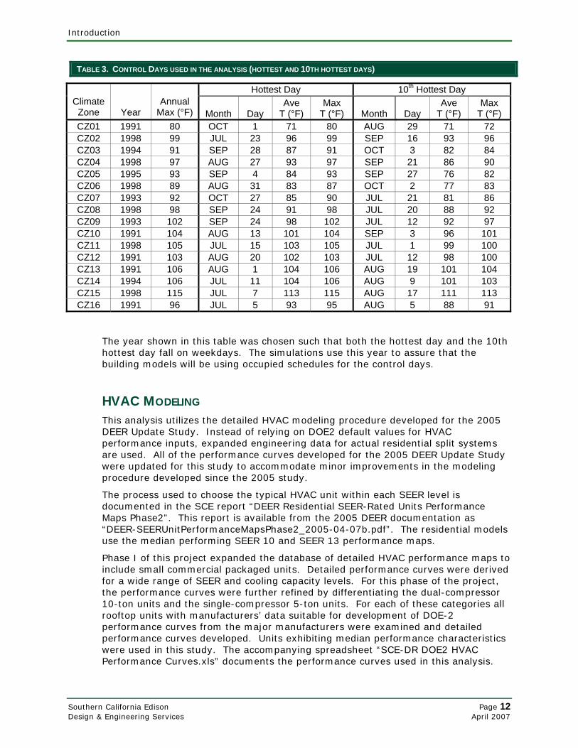
TABLE 3. CONTROL DAYS USED IN THE ANALYSIS (HOTTEST AND 10TH HOTTEST DAYS)

Hottest Day 10th Hottest Day Climate

Zone Year Annual

Max (°F) Month Day Ave

T (°F) Max

T (°F) Month Day Ave

T (°F) Max

T (°F) CZ01 1991 80 OCT 1 71 80 AUG 29 71 72 CZ02 1998 99 JUL 23 96 99 SEP 16 93 96 CZ03 1994 91 SEP 28 87 91 OCT 3 82 84 CZ04 1998 97 AUG 27 93 97 SEP 21 86 90 CZ05 1995 93 SEP 4 84 93 SEP 27 76 82 CZ06 1998 89 AUG 31 83 87 OCT 2 77 83 CZ07 1993 92 OCT 27 85 90 JUL 21 81 86 CZ08 1998 98 SEP 24 91 98 JUL 20 88 92 CZ09 1993 102 SEP 24 98 102 JUL 12 92 97 CZ10 1991 104 AUG 13 101 104 SEP 3 96 101 CZ11 1998 105 JUL 15 103 105 JUL 1 99 100 CZ12 1991 103 AUG 20 102 103 JUL 12 98 100 CZ13 1991 106 AUG 1 104 106 AUG 19 101 104 CZ14 1994 106 JUL 11 104 106 AUG 9 101 103 CZ15 1998 115 JUL 7 113 115 AUG 17 111 113 CZ16 1991 96 JUL 5 93 95 AUG 5 88 91

The year shown in this table was chosen such that both the hottest day and the 10th hottest day fall on weekdays. The simulations use this year to assure that the building models will be using occupied schedules for the control days.

HVAC MODELING This analysis utilizes the detailed HVAC modeling procedure developed for the 2005 DEER Update Study. Instead of relying on DOE2 default values for HVAC performance inputs, expanded engineering data for actual residential split systems are used. All of the performance curves developed for the 2005 DEER Update Study were updated for this study to accommodate minor improvements in the modeling procedure developed since the 2005 study.

The process used to choose the typical HVAC unit within each SEER level is documented in the SCE report “DEER Residential SEER-Rated Units Performance Maps Phase2”. This report is available from the 2005 DEER documentation as “DEER-SEERUnitPerformanceMapsPhase2_2005-04-07b.pdf”. The residential models use the median performing SEER 10 and SEER 13 performance maps.

Phase I of this project expanded the database of detailed HVAC performance maps to include small commercial packaged units. Detailed performance curves were derived for a wide range of SEER and cooling capacity levels. For this phase of the project, the performance curves were further refined by differentiating the dual-compressor 10-ton units and the single-compressor 5-ton units. For each of these categories all rooftop units with manufacturers’ data suitable for development of DOE-2 performance curves from the major manufacturers were examined and detailed performance curves developed. Units exhibiting median performance characteristics were used in this study. The accompanying spreadsheet “SCE-DR DOE2 HVAC Performance Curves.xls” documents the performance curves used in this analysis.


Demand Savings

The base case thermostat schedules described above were used to establish the HVAC demand in the absence of thermostat control. For each base case thermostat simulation, 21 additional simulations were conducted that increase thermostat set point by 4 degrees during the control periods described in table 2.

The demand reduction is determined by comparing the baseline hourly demand to the hourly demand of the control day using the modified thermostat schedule. The demand savings are calculated as the simple difference in hourly energy use from one scenario to the other, normalized by the cooling capacity in tons.

DEMAND SAVINGS The challenge of presenting more than 750,000 sets of results is how to do so in a meaningful and useful way without overwhelming the viewer with too many tables and graphs. This report will present examples of results formats that are available via the spreadsheets accompanying this report. These spreadsheets summarize the results by building type and climate zone while filtering the data based on control period, vintage, thermostat scenario and HVAC sizing. Tools within the spreadsheets facilitate creating tables of results for specific scenarios that are of interest to the user. The spreadsheets also present interactive graphs that allow for the examination and comparison of each individual set of results.

RESULTS SPREADSHEET - SETUP The main results of this analysis must be viewed using the results spreadsheet “SCE-DR_Results_Viewer.xls”. The sheer volume of data generated by this project requires the data to be broken down by building type and climate zone for use with Excel. This main spreadsheet imports individual data files that contain the building and climate zone specific results as needed.

Each building type has 32 associated CSV files: one hourly data set for each climate zone and one annual data set for each climate zone. The data files for a particular building type can be identified by the three letter code used in the file name:

SCE-DR_Asm-Annual-CZ01.csv SCE-DR_Asm-Hourly-CZ01.csv

The climate zone is identified by the last two characters before the file extension. Table 4 lists the three letter codes used for the building types.

All of the data files should reside in the same directory as the main spreadsheet. Also, since the user may want to save the spreadsheet with a new set of data files loaded, the files should not reside on a CD, DVD or other non-rewriteable drive.


Demand Savings

TABLE 4. BUILDING TYPE CODES USED IN CSV SUPPORT FILE

BUILDING TYPE CODE

Assembly ASM

Education - Primary EPr

Education – Secondary ESe

Education - College ECC

Education - University EUn

Education – Relocatable ERe

Grocery Gro

Nursing Home Nrs

Hotel Htl

Motel Mtl

Manufacturing – Light MLI

Manufacturing – MBT

Restaurant - Fast Food RFF

Restaurant – Sit Down/Full RSD

Retail – Large (Big Box) RtL

Storage – Conditioned Sto

Residential - Multifamily MFm

RESULTS SPREADSHEET – GUIDED TOUR The main purpose of the results spreadsheet it to provide the user with a quick and easy oversight of the data of interest as well as provide tables that contain the detailed results needed. As such, the spreadsheet does a fair amount of data manipulation: importing data, sorting data sets, automatically creating formatted tables, etc. The spreadsheet has been tested and used extensively, but it is not necessarily “bomb-proof”. If the spreadsheet gets stuck or appears badly formatted, exit the spreadsheet without savings and start again. If a problem persists, please inform the authors and the problem will be investigated.

Each of the tabs of the spreadsheet will be described and their use explained in the sections below. In general, it will be necessary to choose a scenario when examining the results. “Exploring the data sets” may be a more accurate term to describe how the spreadsheet is used. The large number of individual results (more than 750,000) makes it highly unlikely that a user will view all of the available data. The following options are specified on most of the spreadsheet tabs to define the particular data set that is being explored:

Building Type: the user will need to choose one of the 17 building types (except in the case of comparing results across all building types). Choosing a new building type will cause the spreadsheet load a new data

file


Results Spreadsheet: [Intro] tab

Climate Zone: the user may need to choose one of the 16 climate zone (except in the case of comparing results across all climates) Choosing a new Climate Zone type will cause the spreadsheet load a new

data file

Control Period: One of the 21 control periods may need to be chosen. The start and stop times of each control period are clearly marked.

Building Vintage: One of the three building vintages will typically need to be specified. A fourth option of “weighted” is also available.

Cooling set point: Thermostat controls associated with “high” and “low” or “average” setting can be specified.

For residential building types, another option of “Title-24” is available.

Cooling size ratio: For commercial building types two sizing ratios are available, along with the averaged sizing ratio.

Control Day type: in some cases the control day type of “Hottest Day” or “10th Hottest Day” must be specified, but in most cases both results are displayed or tabulated.

Each of the tabs of the results spreadsheet will be described and their use explained in the sections below.

RESULTS SPREADSHEET: [INTRO] TAB

The first tab of the spreadsheet offers a short description of each of the useful tabs within the spreadsheet. This is a quick guide for those without the benefit of this document.

RESULTS SPREADSHEET: [ALL BUILDINGS] TAB

The [All Buildings] tab offers a quick comparison of demand savings across all building types for a specific climate zone and a chosen building scenario. The user needs to specify the Climate Zone, Control Period, Building Vintage, Cooling Setpoint, and Cooling Size Ratio via the pull-down lists:

FIGURE 1. [ALL-BUILDINGS] CONTROLS

Once the scenario has been chosen, the user needs to press the “Create All-Buildings Table” button. The spreadsheet will proceed to import the results files for the chosen climate zone and for each building type, calculate the summary results and add the


Results Spreadsheet: [All Buildings] tab

results to the summary table. When the process is complete, the graphic will display the new results, as shown in Figure 2. The process of importing all of the necessary data can take a few minutes, during which time the user will see an hourglass cursor.

FIGURE 2. [ALL-BUILDINGS] SUMMARY GRAPHIC

This graphic shows the average demand savings per ton of PCT-controlled DX rooftop units for the entire building and for the chosen scenario. The scenario is listed in the second title line, and in this case the control period is from 2 p.m. to 6 p.m., the vintage specific results are weighted (by the vintage weights specified in the spreadsheet), the cool setpoint specific results are averaged (across the two setpoint scenarios) and the size ratio specific results are averaged (across the two sizing scenarios).

The dark blue column is the first hour savings on the hottest day and the light blue column is the average savings over the entire control period. The dark green column is the first hour savings on the 10th hottest day and the light green column is the average savings over the entire control period on the 10th hottest day.

A table containing hourly results is also produced (Figure 3 shows an image of the table). The table lists the hourly demand results for all hours from noon to midnight. Savings during the hours before the control period starts should always be zero (and are formatted as blank cells) but the hours after the control periods end are typically slightly negative, as the cooling system recovers from the elevated space temperatures during the control hours.


Results Spreadsheet: [All Buildings] tab

FIGURE 3. [ALL BUILDINGS] SUMMARY TABLE


Results Spreadsheet: [All Climates] tab

The table lists the first hour and control period minimum and maximum demand savings (columns 3 through 8). These values reflect the extremes of each individual zone within the building. The range of minimum and maximum give an indication of how robust the demand savings is for individually PCT-controlled rooftop units within the whole building. The table also indicates the energy savings associated with the HVAC system control in kWh per ton of PCT-controlled capacity (last column). This value reflects the overall savings for the entire control period and includes the HVAC rebound effect that may exist once the control period ends.

The [All Buildings] tab is formatted to be printed on two pages, one with the graphic and explanatory text and one with the large table.

From this tab of the worksheet, the user can also cause a much larger table to be generated. Pressing the “Create AllBldg-AllCZ Table” button will cause results for the currently chosen scenario to be generated for all climate zones as well as all building types. A table with 544 rows of data will be created on the [AllBldg-AllCZ] tab. The table is formatted to be printed onto eight pages. The process of creating this table is quite lengthy, as all 544 data files need to be imported and processed. Before executing, the program will warn the user that the process may take 30 to 90 minutes to complete.

Note that, as with many of the tabs, there are hidden columns and rows that are utilized in the creation of the summary table. Care should be taken not to delete, modify or move these cells, as the macros that create the table would likely no longer work.

RESULTS SPREADSHEET: [ALL CLIMATES] TAB

The [All Climates] tab offers a quick comparison of demand savings across all climates for a specific building type and a chosen building scenario. Similar to the [All Buildings] worksheet, the user needs to specify the Building Type, Control Period, Building Vintage, Cooling Setpoint, and Cooling Size Ratio via the pull-down lists. When the “Create All CZ Table” button is pressed, macros will automatically create the table and graphics comparing results for one building type across all climate zones.

As with the “All-Buildings” process, it will take the program a few minutes to complete the process of importing the data sets for all 16 climate zones. When the process is complete, the graph shown in Figure 4 will be updated.



FIGURE 4. [ALL CLIMATES] SUMMARY GRAPHIC

The format of the graph is identical to the “All Buildings” graphic. This graphic plots the average demand savings per ton of PCT-controlled DX rooftop units for the entire building and for the chosen scenario. The dark blue column is the first hour savings on the hottest day and the light blue column is the average savings over the entire control period. The dark green column is the first hour savings on the 10th hottest day and the light green column is the average savings over the entire control period on the 10th hottest day.

The summary table on this tab, as shown in figure 5, has the same format as the summary table of the [All Buildings] tab, with the column of building types replaced with climate zones.



FIGURE 5. [ALL CLIMATES] SUMMARY TABLE


Results Spreadsheet: [AllBldg-AllCZ] tab

RESULTS SPREADSHEET: [ALLBLDG-ALLCZ] TAB

This tab holds the rather large table created from the [All Buildings] tab. The table lists the demand savings results for the chosen scenario for all building types and all climate zones. The table is formatted the same as the previously described tables, only without the color highlights.

This table may be the most appropriate means of gathering all the information of interest into a set of static tables that can then be used for other research or planning projects. The information in this worksheet is formatted to be printed onto eight pages.

FIGURE 6. EXAMPLE OF [ALLBLDG-ALLCZ] TABLE (PARTIAL)


Results Spreadsheet: [All Control Periods] tab

RESULTS SPREADSHEET: [ALL CONTROL PERIODS] TAB

This tab shows how the demand impact for a given scenario varies based on the demand control period. The scenario of building type, climate zone, cooling set point and sizing ration is chosen via the usual pull-down menus.

Changing the building type or climate zone will cause a new data set to be loaded; this will take 20 or 30 seconds. Changing any of the other parameters will delete the currently displayed data. Once all of the parameters have been set, the user must press the “Create Table” button to populate the graphic and table with new results.

FIGURE 7. [ALL CONTROL PERIODS] LARGE RETAIL GRAPHIC

A lot of information is contained in this one graphic. The demand savings of all control periods are shown here, grouped by the control period starting hour. The blue columns show the demand savings when controls are applied on the hottest day of the year. The green columns indicated the demand savings on the 10th hottest day of the year. The darker columns highlight the first-hour demand savings.

Figure 7 shows the demand savings for a large retail building in climate zone 13, with weighted vintage, averaged cooling thermostat set point and averaged HVAC sizing. Some observations based on this graphic:

First hour demand savings is somewhat insensitive to the control day in the early and late afternoon, but is higher for the cooler control day in mid-afternoon.


Results Spreadsheet: [All Control Periods] tab

The highest demand savings occurs in the late afternoon for both the hottest and 10th hottest control days.

There is a 20 – 30% drop in demand savings after the first hour. On the hottest day, the demand savings after the first hour drop remains steady from 2p.m. to 5 p.m.; on the 10th hottest day the demand savings continues to decline as the control period is extended.

These observations are specific to the building configuration being examined. For another example, Figure 8 shows the results for an apartment building in Oakland with a 76°F cooling setpoint:

FIGURE 8. [ALL CONTROL PERIODS] MULTIFAMILY GRAPHIC

In this case, the demand savings potential increases from almost none in the early afternoon to peak values in the late afternoon. Starting the control period at 3p.m. instead of 2p.m. increases the first hour demand savings potential by 50% or more.

Figure 9 illustrates the table showing the hourly demand reduction of each control period presented on this tab. As with previous tables, the hourly results are extended to midnight to show any increase in demand after the control period ends.


FIGURE 9. [ALL CONTROL PERIODS] TABLE SHOWING ALL CONTROL PERIODS

RESULTS SPREADSHEET: [ZONE GRAPHICS] TAB

The graphics on this tab allow the user to explore the thermostat control simulations in depth. This exploration serves as a quality-control exercise more than a results-


Results Spreadsheet: [Zone Graphics] tab

gathering exercise, but may provide valuable insight to anyone needing to rely on the results of this study.

As with most of the other worksheets in this spreadsheet, the user must choose a building scenario through the available pull-down menus that includes all of the usual parameters. Since these graphics display individual simulation results, the weighted and averaged options for cooling set point, sizing ratio and building vintage are not available.

Two additional controls determine which zones are included in the graphs. “Starting Zone Number” and “Number of Zones to Plot” have spin controls associated with them, allowing the user to quickly scroll through all the zones in the building, either one at a time or all on the same graph.

For the chosen scenario, the impacts of PCT control are illustrated in five graphs. Each graph displays hourly profiles for both the base case and the PCT-controlled case. Figure 10 shows the temperature profile graph for a single zone. The space temperature is brought down at 8a.m. and maintained at approximately 72°F throughout the day for the base case. The space temperature for the PCT-controlled case is elevated by about 4°F during the control period, as expected for this scenario.

FIGURE 10. [ZONE GRAPHICS] TEMPERATURE PROFILE

Figure 11 shows the compressor part-load-ratio (PLR) profiles for all the rooftop systems in the Large Retail building. The base case PLR profiles reach a maximum between 0.8 and 1.0 for the given scenario. During the control period the PLR values drop to between 0.4 and 0.7, showing that all the compressors continued to run during each hour, but ran for shorter periods while the thermostat was elevated.


Results Spreadsheet: [Zone Graphics] tab

FIGURE 11. [ZONE GRAPHICS] PART LOAD RATIO PROFILE FOR ALL SYSTEMS

A graphic similar to Figure 11 shows the compressor kW profiles. These profiles differ slightly from the PLR profiles due to changes in the HVAC performance as a function of part load.

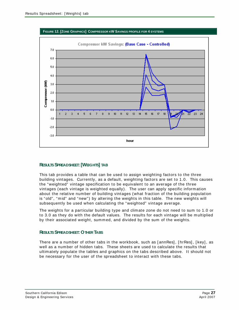
The compressor kW savings graphic, shown in Figure 12, illustrates the change in electric demand for the zones (and therefore systems) chosen. The example shows the kW reduction for four of the HVAC systems in the building.

Finally, a graph shows the outdoor temperature profile for the control day being displayed. Taken together, the graphics provide insight into how the building and HVAC systems respond to the thermostat control. These graphs were referred to extensively while refining the prototypes and simulations for this project.


Results Spreadsheet: [Weights] tab

FIGURE 12. [ZONE GRAPHICS] COMPRESSOR KW SAVINGS PROFILE FOR 4 SYSTEMS

RESULTS SPREADSHEET: [WEIGHTS] TAB

This tab provides a table that can be used to assign weighting factors to the three building vintages. Currently, as a default, weighting factors are set to 1.0. This causes the “weighted” vintage specification to be equivalent to an average of the three vintages (each vintage is weighted equally). The user can apply specific information about the relative number of building vintages (what fraction of the building population is “old”, “mid” and “new”) by altering the weights in this table. The new weights will subsequently be used when calculating the “weighted” vintage average.

The weights for a particular building type and climate zone do not need to sum to 1.0 or to 3.0 as they do with the default values. The results for each vintage will be multiplied by their associated weight, summed, and divided by the sum of the weights.

RESULTS SPREADSHEET: OTHER TABS

There are a number of other tabs in the workbook, such as [annRes], [hrRes], [key], as well as a number of hidden tabs. These sheets are used to calculate the results that ultimately populate the tables and graphics on the tabs described above. It should not be necessary for the user of the spreadsheet to interact with these tabs.


Sensitivity of Demand Savings to HVAC Performance

SENSITIVITY OF DEMAND SAVINGS TO HVAC PERFORMANCE Task 4 of this project set out to determine the sensitivity of the demand response impacts determined in this report to the range of potential HVAC units that may be used in these applications. To this end, performance curves for a large set of units were developed based on both dual compressor 10-ton units and single compressor 5-ton units sold by five different manufactures. A range of units representing high and low performance were then substituted into the demand response analysis for one building type and a subset of climate zones. The subsequent demand response of these units was then compared to the demand response of the median HVAC unit.

PERFORMANCE CURVES Forty-nine sets of demand curves were developed based on both dual compressor 10-ton units and single compressor 5-ton units sold by five different manufactures. The median units from these two categories were identified by comparing the fan and compressor power of each unit, along with the compressor power as a function of outdoor dry bulb temperature and coil entering wet bulb temperature. The median units (median values of fan energy, compressor efficiency, and sensitivity to outdoor dry bulb and coil entering wet-bulb temperatures) were used for all of the demand savings analysis described in this report.

Units that represent the “high” and “low” performance were also identified using these same parameters. These units are identified in table 5. Note that the unit with low fan energy/high EIR is the same unit with the high sensitivity of EIR to outside dry-bulb temperature. The full set of performance curves are documented in the spreadsheet “SCE-DR DOE2 HVAC Performance Curves.xls” that accompanies this report.

TABLE 5. DUAL-COMPRESSOR 10-TON UNITS USED IN HVAC SENSITIVITY ANALYSIS

Description Graph

Legend Make Model EER Rated EIR

Rated Fan

W/CFM Median Unit H1 Lennox LGC120S2 10.63 0.25 0.36 High Fan Energy/Low EIR H2 Goodman PGC120 10.36 0.22 0.63 Low Fan Energy/High EIR H3 Carrier 50GJ012 (R407C) 10.49 0.28 0.22 High Sensitivity of EIR to ODB H3 Carrier 50GJ012 (R407C) 10.49 0.28 0.22 Low Sensitivity of EIR to ODB H4 Carrier 48TM012 9.97 0.27 0.38 High Sensitivity of EIR to EWB H5 York DF102G 9.28 0.25 0.58 Low Sensitivity of EIR to EWB H6 RUUD RLMB-A120 10.11 0.25 0.46

DEMAND IMPACT OF ALTERNATIVE HVAC UNITS The large retail prototype was used to study the effect of different HVAC units on the demand savings of PCTs. The retail prototype was chosen for a number of reasons. First, the large “big box” retail is a relatively well characterized model, with building characteristics and operating schedules that don’t have a large range of possibilities (as compared to Assembly or manufacturing buildings). Second, as shown in Figure 2, the large retail exhibits a typical demand response compared with all building types.



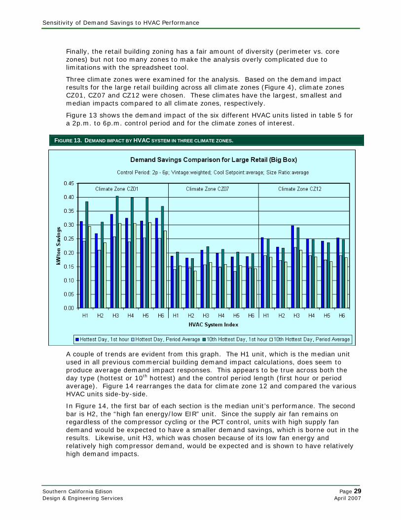
Finally, the retail building zoning has a fair amount of diversity (perimeter vs. core zones) but not too many zones to make the analysis overly complicated due to limitations with the spreadsheet tool.

Three climate zones were examined for the analysis. Based on the demand impact results for the large retail building across all climate zones (Figure 4), climate zones CZ01, CZ07 and CZ12 were chosen. These climates have the largest, smallest and median impacts compared to all climate zones, respectively.

Figure 13 shows the demand impact of the six different HVAC units listed in table 5 for a 2p.m. to 6p.m. control period and for the climate zones of interest.

FIGURE 13. DEMAND IMPACT BY HVAC SYSTEM IN THREE CLIMATE ZONES.

A couple of trends are evident from this graph. The H1 unit, which is the median unit used in all previous commercial building demand impact calculations, does seem to produce average demand impact responses. This appears to be true across both the day type (hottest or 10th hottest) and the control period length (first hour or period average). Figure 14 rearranges the data for climate zone 12 and compared the various HVAC units side-by-side.

In Figure 14, the first bar of each section is the median unit’s performance. The second bar is H2, the “high fan energy/low EIR” unit. Since the supply air fan remains on regardless of the compressor cycling or the PCT control, units with high supply fan demand would be expected to have a smaller demand savings, which is borne out in the results. Likewise, unit H3, which was chosen because of its low fan energy and relatively high compressor demand, would be expected and is shown to have relatively high demand impacts.



FIGURE 14. DEMAND IMPACT BY HVAC SYSTEM IN CLIMATE ZONE 12

Table 6 summarizes the results for all HVAC units in the three climate zones. Overall, the variation in demand impact for different HVAC units as compared to the values reported for the median unit is limited to about ±15%. The reported values based on the median HVAC unit appear to do a good job of indicating the median expected impacts.

TABLE 6. DEMAND SAVINGS (KW/TON) STATISTICS ACROSS ALL HVAC SYSTEMS

All HVAC Units 1st Hr Period 1st Hr Period 1st Hr PeriodMinimum 0.269 0.209 0.180 0.133 0.221 0.172Average 0.314 0.242 0.191 0.144 0.253 0.189Maximum 0.339 0.258 0.209 0.157 0.298 0.220Range 0.070 0.049 0.029 0.024 0.078 0.047

Range High + 8% 6% 9% 9% 18% 16%Range Low ? -14% -14% -6% -8% -13% -9%

CZ01 CZ07 CZ12


Impact of Staged Volume Systems on Demand Savings

IMPACT OF STAGED VOLUME SYSTEMS ON DEMAND SAVINGS As a final step in this project, the potential impact of staged-volume packaged rooftop systems on the demand savings of PCTs is examined. An earlier report “Staged-Volume Phase 1 Report-Energy Savings Potential” describes the concept of staged-volume:

Described briefly, rooftop DX cooling equipment with cooling capacities greater than 7.5 tons most frequently have multiple stages of cooling, e.g., dual compressors or dual stage compressors, but are restricted to constant volume fan operation. The Staged Volume concept recognizes that for the smaller range of these types of systems, say 7.5 to 20 tons, the fan energy resulting from constant volume operation will represent a significant portion of the total annual energy use of the system. Hence, if the fan flow can be staged with the compressor activity, a significant savings in annual energy and operations costs can be realized. If the staged volume control is accomplished using a variable speed drive, there is also a potential for demand savings.

While the HVAC performance modeling in this report is based on the reported performance of actual units, there are no engineering specifications for staged volume systems at this time. As such, assumptions are made regarding the compressor performance and the air-volume staging.

DEMAND IMPACT OF STAGED-VOLUME SYSTEMS The large retail model is again used to study the impact of an alternative HVAC scenario on the demand savings of PCTs. It is assumed that the compressor performance of the staged-volume system is well characterized by the median dual-compressor HVAC unit developed for this study. Greater or less savings may be realized by units with higher or lower fan power versus compressor power, as investigated in the previous chapter.

Figure 15 compares the constant volume and staged volume systems across all climate zones on the hottest day of the year. With few exceptions, the first hour and period average demand savings are significantly higher for the staged volume system.



FIGURE 15. CONSTANT VOLUME AND STAGED VOLUME DEMAND IMPACT ON THE HOTTEST DAY

Figure 16 shows the same results for the 10th hottest day of the year. In this case the results are more consistent, as the staged volume unit is able to operate for longer periods of the control period with the supply fan in reduced speed operation. Table 7 summarizes these comparisons illustrating an average increase in the demand impact of 20% across all climate zones and control days.

While the performance characteristics of staged-volume systems are not yet available for commercially sold units, their ability to reduce electricity demand during periods of reduced load guarantees a positive impact on the demand savings of PCTs.



FIGURE 16. CONSTANT VOLUME AND STAGED VOLUME DEMAND IMPACT ON THE 10TH HOTTEST DAY



TABLE 7. PERCENT INCREASE IN DEMAND SAVINGS DUE TO STAGED VOLUME SYSTEM

Hottest Day 10th Hottest Day Climate 1st Hr Period 1st Hr Period CZ01 10% 1% 7% 0% CZ02 27% 36% 22% 28% CZ03 20% 25% 14% 18% CZ04 13% 16% 15% 22% CZ05 19% 23% 21% 17% CZ06 3% -1% 13% 12% CZ07 8% 11% 16% 23% CZ08 18% 19% 15% 18% CZ09 27% 39% 20% 27% CZ10 15% 17% 14% 9% CZ11 22% 29% 21% 27% CZ12 20% 25% 23% 33% CZ13 12% 26% 29% 41% CZ14 14% 23% 23% 30% CZ15 27% 32% 25% 34% CZ16 20% 29% 17% 24%

average: 16% 21% 18% 23% overall average: 20%


Documents

Impact of PCTs on Demand Response - Phase II · Impact of PCTs on Demand Response – Phase II ACKNOWLEDGEMENTS Southern California Edison’s Design & Engineering Services (D&ES)