Embed Size (px)
Citation preview
Impact of Port Infrastructure Development and Operational Efficiency of Ports on
Export Performance: A study of manufactured product exports from India
Bishwanath Goldar* and Mahua Paul**
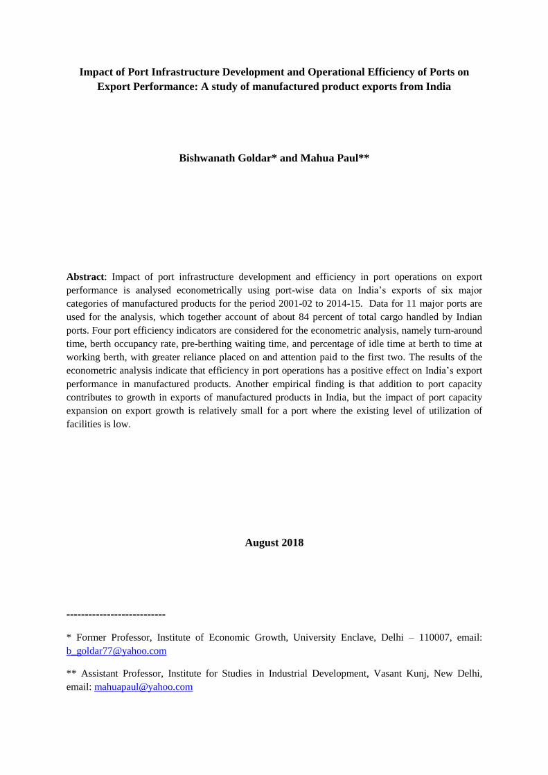
Abstract: Impact of port infrastructure development and efficiency in port operations on export
performance is analysed econometrically using port-wise data on India’s exports of six major
categories of manufactured products for the period 2001-02 to 2014-15. Data for 11 major ports are
used for the analysis, which together account of about 84 percent of total cargo handled by Indian
ports. Four port efficiency indicators are considered for the econometric analysis, namely turn-around
time, berth occupancy rate, pre-berthing waiting time, and percentage of idle time at berth to time at
working berth, with greater reliance placed on and attention paid to the first two. The results of the
econometric analysis indicate that efficiency in port operations has a positive effect on India’s export
performance in manufactured products. Another empirical finding is that addition to port capacity
contributes to growth in exports of manufactured products in India, but the impact of port capacity
expansion on export growth is relatively small for a port where the existing level of utilization of
facilities is low.
August 2018
---------------------------
* Former Professor, Institute of Economic Growth, University Enclave, Delhi – 110007, email:
** Assistant Professor, Institute for Studies in Industrial Development, Vasant Kunj, New Delhi,
email: [email protected]

1
Impact of Port Infrastructure Development and Operational Efficiency of Ports on
Export Performance: A study of manufactured product exports from India
1. Introduction
Development of port infrastructure and efficiency in port operations are expected to play an
important role in enhancing export performance of developing countries. This is so because
better port infrastructure and improved efficiency in port operations will have a favourably
impact on their export competitiveness and thus contribute to exports.1 While this
relationship is recognized in the literature, to the knowledge of the authors of this paper, there
has been very little econometric research on the impact of port capacity augmentation and
improvements in efficiency of port operations on India’s export performance2 (also, it
appears, there have been very few econometric studies on this issue, if any, for other
emerging economies). The present paper makes an attempt in this direction.
The analysis is confined to six broad groups of manufactured products: (i) Chemicals and
chemical products, (ii) Basic metals and metal products, (iii) Machinery, (iv) Transport
equipment, (v) Food products and beverages, and (vi) Textiles including readymade
garments. The annual exports of these items through 11 important ports in India are
considered for the analysis. The ports considered are: Kolkata, Paradip, Vishakhapatnam,
Chennai, Tuticorin, Cochin, New Managalore, Mormugao, Jawaharlal Nehru (Nhava Sheva),
Mumbai and Kandla. The time period covered for the study is 2001-02 to 2014-15.
Taken together, the 11 ports selected for the study account for about 84% of the total traffic
handling capacity of Indian ports. The products considered for the study account for a fairly
large portion of India’s exports of manufactured products.3
1 How hard and soft infrastructure impacts exports performance in developing countries has been studied by Portugal-Perez and Wilson (2010). Also see, in this context, Clark et al. (2004), Nordas et al. (2006) and Iwanow and Kirkpatrick (2008). 2 This issue has been examined for India by Ghosh and De (2002) using data on Indian ports and applying a production function framework. They considered the period 1985-86 to 1996-97. An investigation into the causality between port performance and traffic handled in Indian ports has been undertaken by De and Ghosh (2003) using data for the period 1985-86 to 1999-2000. Also see, De (2009). 3 Two important groups of products produced by the Indian manufacturing sector and exported from India which have not been included in the econometric analysis are (a) petroleum refinery products and (b) gems and jewellery. Both of them are characterized by a high degree of import dependence. It may be mentioned in this connection that in several empirical studies on India’s manufactured exports, petroleum refinery products have not been considered for the analysis (see, for instance, Francis, 2015 and Veeramani, et al., 2017). The exclusion of petroleum products from the econometric analysis in this study therefore seems justified. As

2
The paper is organized as follows. The next section, i.e. Section 2, describes the trends in port
capacity, actual traffic handled and the rate of capacity utilization in the Indian ports,
followed by an analysis of trends in capacity utilization and port operational efficiency in the
11 major ports selected for the study. The period covered is 2001-024 (at places written as
2001) to 2014-15 (2014). This serves as a background to the econometric analysis presented
subsequently in the paper.
Section 3 is devoted to an econometric analysis of the impact of port capacity development
and port operational efficiency on manufactured products export performance in India. In
this case again the period covered is 2001-02 to 2014-15. This section is divided into three
subsections. Section 3.1 deals of with data sources and variables, and Section 3.2 with
econometric methodology (i.e. specification of econometric models). Section 3.3 presents the
econometric results, i.e. the model estimates. Finally, Section 4 summarises the main findings
of the study and concludes.
2. Trend Analysis: Port Capacity, Capacity Utilization and Efficiency in Operations
2.1 Port Capacity and Traffic Handled
Figure 1 shows the trends in port capacity and traffic handled in the ports in India in the
period 2001-02 to 2014-15 (presenting trends at the aggregate level covering all Indian ports).
It is evident that there has been a steady increase in port capacity. The trend growth rate in
port capacity during 2001-02 to 2014-15 was about 7.3 percent per annum. Between 2001-02
and 2007-08, the increases in traffic handled by and large matched the increases in port
capacity. However, in subsequent years, while the port capacity has steadily increased, the
increase in traffic handled has been rather modest, leading to a significant fall in capacity
utilization. Between 2001-02 and 2014-15, capacity utilization (ratio of traffic handled to port
capacity) fell by about 17 percentage points, from about 84% in 2001-02 to about 67% in
regards gems and jewellery, Francis (2015) has included these products in her analysis of India’s manufactured exports. Veeraamani et al. (2017), in their study of India’s manufactured exports, have left out SITC 667(Pearls and precious or semi-precious stones, un-worked or worked) but have included SITC 897 (Gold, silver ware, jewelry and articles of precious materials, n.e.s.). In this study, however, gems and jewellery have been excluded from the econometric analysis. It was felt that since the study is focused on the use of sea port facilities, it would not be appropriate to estimate a common export function by pooling export data on products which are low weight and very high in value (e.g. gold ornaments) with such data for traditional manufactured export products (e.g. textiles or shoes) which do not share this characteristic. 4 This is financial year, from April 2001 to March 2002. Similarly, 2014-15 is the financial year from April 2014 to March 2015.

3
2015-16. It should be pointed out that capacity utilization improved between 2001-02 and
2007-08. It reached 98% in 2007-08, and the fall in subsequent years, 2007-08 to 2014-15,
was therefore quite sharp.
Source: Prepared by authors based on data taken from Annual Report, 2016-17, Ministry of Shipping,
Government of India (Table 4.32, p.30).
The slowdown in the growth rate in traffic handled through sea ports in the period after 2007
seems to have a lot to do with the recessionary conditions prevailing in India post-2007
which is rooted in the global economic crisis. Figure 2 contrasts traffic handled in Indian
ports with the volume index of India’s exports and imports5 for the period 2001-02 to 2014-
15. It is interesting to note that the volume index of exports has maintained an upward trend
at more or less at the same pace after 2007-08, but the volume index of imports declined
markedly after 2010-11. Evidently, it is the decline in import traffic handled at ports that has
caused the overall traffic at ports to stagnate after 2010-11. In spite of the stagnation in the
volume of import traffic handled at ports, the pace of port capacity development has
5 The volume indices of exports and imports are brought out by the DGCIS (Directorate General of Commercial Intelligence and Statistics), Government of India.
0
100
200
300
400
500
600
700
800
900
1000
20
01
-02
20
02
-03
20
03
-04
20
04
-05
20
05
-06
20
06
-07
20
07
-08
20
08
-09
20
09
-10
20
10
-11
20
11
-12
20
12
-13
20
13
-14
20
14
-15
mill
ion
to
nn
es
Fig. 1: Port capacity and traffic handled in Indian ports, 2001-02 to 2014-15
Port capacity
Traffic handled

4
continued after 2010-11 with the consequence that the rate of capacity utilization has come
down.
Note: Volume indices of exports and imports (1999-2000=100) are shown along right scale. Traffic
handled is shown along left scale.
Source: Prepared by authors based on data taken from Annual Report, 2016-17, Ministry of Shipping,
Government of India (Table 4.32, p.30) and Economic Survey, 2016-17, Ministry of Finance,
Government of India, Volume-2, (Table 7.6, p. A127).
Port-wise details in regard to growth in capacity, growth in traffic handled, change in
capacity utilization and growth in deflated value of manufactured exports are provided in
Table 1 in respect of the 11 ports covered in the study. The table brings out that, between
2001-02 and 2014-15, there was a significant fall in capacity utilization in 9 out of the 11
ports considered for this study, consistent with the trends observed in Figure 1. A relatively
bigger fall in capacity utilization took place in Mormugao, Cochin, Vishakhapatanam, New
Managalore and Chennai ports.
The trend growth rate in capacity during 2001-02 to 2014-15 was relatively high in the
following ports: Kandla, Cochin, New Mangalore, Paradip, Tuticorin and Jawaharlal Nehru.
Among these, the trend growth rate in traffic handled was close to the trend growth rate in
0
50
100
150
200
250
300
350
400
450
0
100
200
300
400
500
600
700
20
01
-02
20
02
-03
20
03
-04
20
04
-05
20
05
-06
20
06
-07
20
07
-08
20
08
-09
20
09
-10
20
10
-11
20
11
-12
20
12
-13
20
13
-14
20
14
-15
mill
ion
to
ne
s
Figure 2: Traffic Handled in Indian Ports (left scale) and Volume Index of India's Exports and Imports (right scale,
1999-2000=100)
Traffic handled
Volume index of exports
Volume index of imports
5
capacity in Kandla, Paradip, Tuticorin and Jawaharlal Nehru. Thus, in two cases, Cochin and
New Mangalore, a relatively high growth rate in capacity was not accompanied by a
relatively high growth rate in traffic handled. Consequently, capacity utilization fell
significantly in these two ports. In Mumbai port, by contrast, there was not much increase in
port capacity whereas traffic handled kept growing which resulted in a significant increase in
capacity utilization.
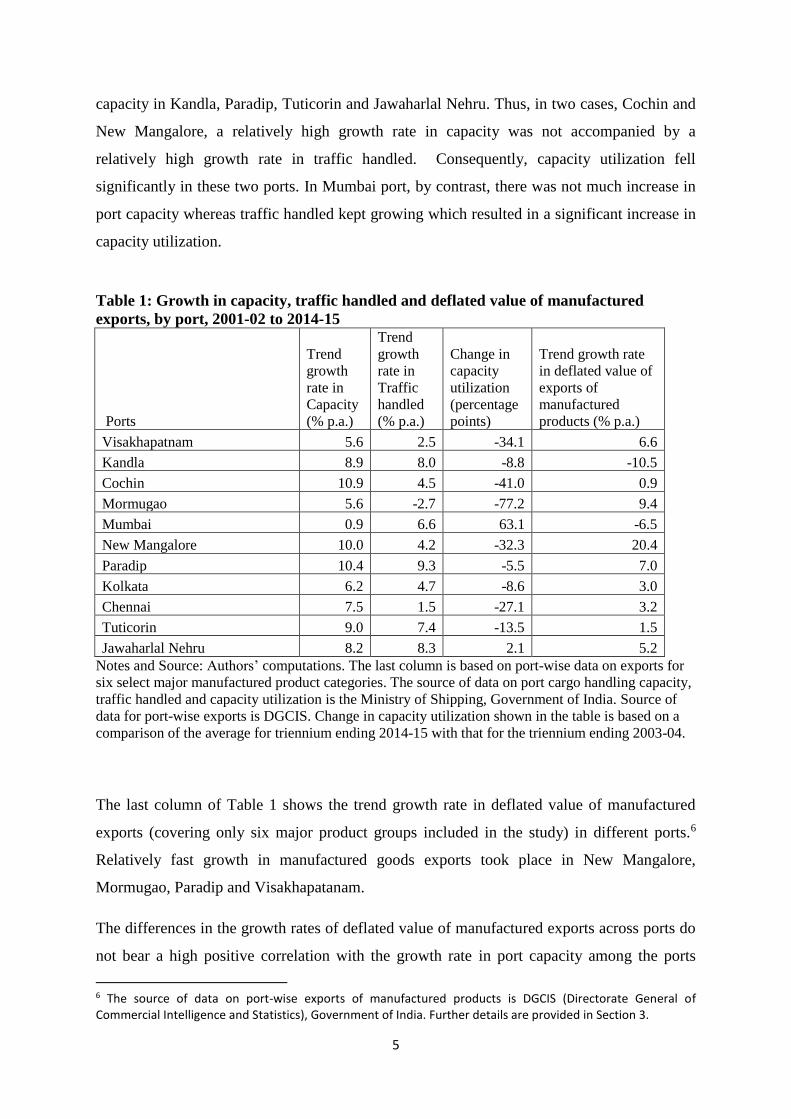
Table 1: Growth in capacity, traffic handled and deflated value of manufactured
exports, by port, 2001-02 to 2014-15
Ports
Trend
growth
rate in
Capacity
(% p.a.)
Trend
growth
rate in
Traffic
handled
(% p.a.)
Change in
capacity
utilization
(percentage
points)
Trend growth rate
in deflated value of
exports of
manufactured
products (% p.a.)
Visakhapatnam 5.6 2.5 -34.1 6.6
Kandla 8.9 8.0 -8.8 -10.5
Cochin 10.9 4.5 -41.0 0.9
Mormugao 5.6 -2.7 -77.2 9.4
Mumbai 0.9 6.6 63.1 -6.5
New Mangalore 10.0 4.2 -32.3 20.4
Paradip 10.4 9.3 -5.5 7.0
Kolkata 6.2 4.7 -8.6 3.0
Chennai 7.5 1.5 -27.1 3.2
Tuticorin 9.0 7.4 -13.5 1.5
Jawaharlal Nehru 8.2 8.3 2.1 5.2
Notes and Source: Authors’ computations. The last column is based on port-wise data on exports for
six select major manufactured product categories. The source of data on port cargo handling capacity,
traffic handled and capacity utilization is the Ministry of Shipping, Government of India. Source of
data for port-wise exports is DGCIS. Change in capacity utilization shown in the table is based on a
comparison of the average for triennium ending 2014-15 with that for the triennium ending 2003-04.
The last column of Table 1 shows the trend growth rate in deflated value of manufactured
exports (covering only six major product groups included in the study) in different ports.6
Relatively fast growth in manufactured goods exports took place in New Mangalore,
Mormugao, Paradip and Visakhapatanam.
The differences in the growth rates of deflated value of manufactured exports across ports do
not bear a high positive correlation with the growth rate in port capacity among the ports
6 The source of data on port-wise exports of manufactured products is DGCIS (Directorate General of Commercial Intelligence and Statistics), Government of India. Further details are provided in Section 3.

6
considered. The highest growth rate in manufactured exports is observed for New Mangalore
port at about 20 percent per annum. This port achieved substantial increase in capacity
between 2001-02 and 2014-15, at the rate of about 10 percent per annum. By contrast,
capacity and traffic handled at Kandla port grew respectively at 8.9 and 8.0 percent per year,
but the real value of exports of manufactured products decreased at the rate of about 10.5
percent per year.7
2.2 Operational Efficiency of Ports
To analyse trends in operational efficiency of Indian ports, four port efficiency indicators
have been chosen for the study (data source: www.Indiastat.com8 which provides data on port
efficiency/ performance indicators compiled from official sources). These indicators reflect
the efficiency with which the port infrastructure is being operated.
Of the various indicators available, the following two receive greater attention in the study:
turn-around time (TRT) and berth occupancy rate (BOR). TRT is the time spent by a vessel
at the port from its arrival at the reporting station to its departure from the reporting station.
The average TRT for all vessels served at the port during a year (measured in number of
days) is used for the analysis. The second indicator, i.e. BOR, is measured as a ratio of time a
berth is occupied by a vessel to the total time available during a period. This is a measure of
the degree of utilization of port facilities. A high berth occupancy rate is a sign of port
congestion, while a low berth occupancy rate signifies low utilization of the facilities
available.
Besides the two above-mentioned indicators of port efficiency, two other indicators used for
the analysis are pre-berthing waiting time or detention (PBD) and percentage of idle time
(PIT).9 PBD is a part of TRT and is measured as the number of days of detention/delay
before berthing of vessels, on average during the year. Needless to say that a higher PBD or
TRT signifies greater inefficiency. PIT is the percentage of idle time at berth to time at
working berth.
7 A closer look at the port-wise exports data reveals that exports of machinery through Kandla port declined significantly between 2001-02 and 2014-15. This largely explains the significant fall in manufactured exports through Kandla port during 2001-2014. 8 The basic source of port performance data available at the website www.Indiastat.com is the Ministry of Shipping, Government of India. 9 The four indicators chosen in this study for analysis are often used for assessing port efficiency and performance. These have been used by Ghosh and De (2002), De and Ghosh (2003) and De (2009) for the analysis undertaken by them. Some of the other indicators considered by De and Ghosh in their studies include output per ship-berth-day, operating surplus per tonne of cargo handled and the rate of return on turnover.

7
For the trend analysis presented in this section of the paper, another indicator of efficiency is
considered. This is the operating surplus. Operating surplus is normalized by cargo handled.
Thus, the variable considered for the analysis is operating surplus per tonne of cargo handled
(PTOS) (in Rs) with adjustment made for inflation.10
Figures 3-7 show changes in port efficiency/ performance indicators over time. It is evident
from Figures 3 that there was an upward trend in turn-around time during 2001-02 to 2010-
11, which was followed by a downward trend during 2011-12 to 2014-15.11 In operating
surplus per tonne of cargo handled, there was an upward trend during 2001-02 to 2006-07,
and a downward trend thereafter. Overall, there is a negative correlation between the time
series on turn-around time and that on operating surplus per tonne. The correlation
coefficient is (-)0.41.12
Source: Authors’ computations. Data on port performance indicators have been taken from
Indiastat.com. The basic source of these data is the Ministry of Shipping, Government of India.
10 To make adjustments for inflation, the data on PTOS have been deflated by the all commodities wholesale price index. 11 Average TRT considering all Indian ports fell from 8.10 days in 1990-91 to 3.63 days in 2005-06. It then increased to 5.29 days in 2010-11 (consistent with the pattern visible in Figure 3). After 2010-11, there was a downward trend in TRT. It came down to 3.64 in 2015-16. See Update on Indian Port Sector (31.03.2017), Transport Research Wing, Ministry of Shipping, Government of India. 12 There is a significant positive correlation between operating surplus and capacity utilization. The correlation coefficient between capacity utilization and inflation-corrected operating surplus per tonne of cargo handled is found to be 0.73.
0
10
20
30
40
50
60
0
1
2
3
4
5
6
Fig.3: Turn-around time and operating surplus, average for 11 major ports
OS per tonne, Rs. (right scale)
TRT in days (left scale)
8
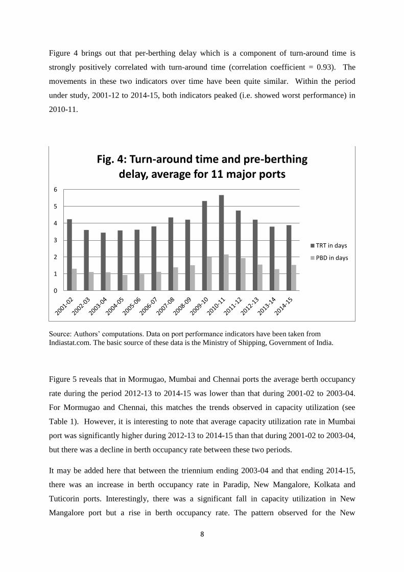
Figure 4 brings out that per-berthing delay which is a component of turn-around time is
strongly positively correlated with turn-around time (correlation coefficient = 0.93). The
movements in these two indicators over time have been quite similar. Within the period
under study, 2001-12 to 2014-15, both indicators peaked (i.e. showed worst performance) in
2010-11.
Source: Authors’ computations. Data on port performance indicators have been taken from
Indiastat.com. The basic source of these data is the Ministry of Shipping, Government of India.
Figure 5 reveals that in Mormugao, Mumbai and Chennai ports the average berth occupancy
rate during the period 2012-13 to 2014-15 was lower than that during 2001-02 to 2003-04.
For Mormugao and Chennai, this matches the trends observed in capacity utilization (see
Table 1). However, it is interesting to note that average capacity utilization rate in Mumbai
port was significantly higher during 2012-13 to 2014-15 than that during 2001-02 to 2003-04,
but there was a decline in berth occupancy rate between these two periods.
It may be added here that between the triennium ending 2003-04 and that ending 2014-15,
there was an increase in berth occupancy rate in Paradip, New Mangalore, Kolkata and
Tuticorin ports. Interestingly, there was a significant fall in capacity utilization in New
Mangalore port but a rise in berth occupancy rate. The pattern observed for the New
0
1
2
3
4
5
6
Fig. 4: Turn-around time and pre-berthing delay, average for 11 major ports
TRT in days
PBD in days

9
Mangalore port is opposite to that observed for Mumbai port. Clearly, there is a mismatch
between inter-temporal movements in capacity utilization and berth occupancy rate for
Mumbai port and New Mangalore port. At the same time, it should be noted that if the other
nine ports are considered ignoring Mumbai and New Mangalore ports, the port-wise changes
in capacity utilization rate are found to be strongly positively correlated with those in berth
occupancy rate. The correlation coefficient is about 0.85. Thus, the general pattern observed
is that increase in berth occupancy rate is associated with better capacity utilization.
Source: Authors’ computations. Data on port performance indicators have been taken from
Indiastat.com. The basic source of these data is the Ministry of Shipping, Government of India.
Figure 6 portrays the trends in capacity utilization and berth occupancy rate over time taking
the average value for the 11 ports considered for the study. Some similarly in movements is
observed. The correlation coefficient is 0.32. Between 2001-02 and 2007-08, there was an
increase in both capacity utilization and berth occupancy rate. In the subsequent period, the
trends are somewhat dissimilar. While there was a clear downward trend in average capacity
utilization rate across ports between 2007-08 and 2014-15, the fall in average berth
occupancy rate has been modest.
0 20 40 60 80
Visakhapatnam
Kandla
Cochin
Mormugao
Mumbai
N.Mangalore
Paradip
Kolkata
Chennai
Tuticorin
J.L.Nehru
Fig. 5: Berth Occupancy rate, by port, 2012-2014 average compared with 2001-2003
average
2012 to 2014 average
2001 to 2003 average

10
Source: Authors’ computations. Data on Berth occupancy rate have been taken from Indiastat.com.
The basic source of these data is the Ministry of Shipping, Government of India. Data on capacity
utilization have been drawn from documents of the Ministry of Shipping.
Figure 7 shows, similarly, the trends in berth occupancy rate and percentage of idle time
taking average value for the 11 ports considered for the study. The movements in the two
indicators over time are by and large in the opposite direction. The correlation coefficient is
(-)0.47. In the period 2001-02 to 2007-08, there was an increase in average berth occupancy
rate and a downward trend in port-wise average of idle time (percentage of idle time at berth
to time at working berth). Between 2007-08 and 2014-15, average berth occupancy rate fell
and the port-wise average of percentage of idle time went up slightly.
0
20
40
60
80
100
120
pe
rce
nt
Fig. 6: Capacity utilization and Berth occupancy rate, 2001-02 to 2014-15, average
across 11 major ports
Capacity utilization
Berth occupancy rate

11
Source: Authors’ computations. Data on Berth occupancy rate and idle time have been taken from
Indiastat.com. The basic source of these data is the Ministry of Shipping, Government of India.
3. Econometric Analysis
3.1 Data Sources
The study uses a dataset on port-wise exports of different categories of products, which has
been obtained from the DGCIS (Directorate General of Commercial Intelligence and
Statistics, Government of India). The dataset provides disaggregated product-level (two-digit
HS [Harmonized System]) data on exports for different ports. The data for six major
manufactured product groups mentioned in the introductory section of the paper above are
used for the analysis.13 This is perhaps the first econometric study on manufactured exports
using disaggregated port-wise export data for India.
An econometric model has been estimated to explain port- and product-wise variation in the
level of manufactured exports over time. The value of exports of the six product groups has
13 The two-digit product categories according to HS (Harmonized System) included in the analysis are: Chemicals and chemical products (28-38); Metals and metal products (72-83); Machinery (84-85); Transport equipment (86-89); Textiles (50-63) and Food products and beverages (16-24).
0
10
20
30
40
50
60
70
80
pe
rce
nt
Fig. 7: Berth occupancy rate and percentage of idle time, 2001-02 to 2014-15, average for 11
ports
Berth occupancy rate
Percentage of idle time

12
been deflated to adjust for inter-temporal changes in export prices and derive a measure of
export quantity (or volume). For this purpose, the unit value index for the relevant product
category has been used (source: DGCIS).
The explanatory variables considered for the econometric model are:
• World exports of the relevant product category in US dollars (source: UNCTAD stat)
• Domestic production of the relevant product category in the state in which the port is
located and in neighbouring states (source: Annual Survey of Industries (ASI), Central
Statistics Office, Government of India). The data on value of domestic production has
been deflated by the corresponding wholesale price index. Since the ASI data have
been used for constructing this variable, it captures the production in the organized
sector segment of the relevant industry.14 This is hereafter referred to as deflated
regional production of the product category.
• Real effective exchange rate (source: Reserve Bank of India). It is computed by the
Reserve Bank of India on the basis of export-based bilateral exchange rates for 36
countries.
• Port operational efficiency indicators. Four indicators are used, namely turn-around
time (TRT), berth occupancy rate (BOR), pre-berthing waiting time or detention
(PBD) and percentage of idle time (PIT). These indicators have been explained in
Section 2. The data on these variables have been drawn from Indiastat.com which
compiles these data from official sources.
An alternate econometric model that has been estimated for additional analysis aims at
explaining port- and product-wise variation in the growth rate in exports over time. In this
model, the growth rate in port capacity is introduced as an explanatory variable along with
growth rates or rates of change in regional production, international demand (captured by
global exports of the relevant product category), real effective exchange rate and port
efficiency indictors.
14 The fact that production data relate to the organized sector and leave out production in the unorganized sector is a limitation of the study. It should be pointed out, however, that from the available data sources, one cannot get state-wise industry-wise value of output in unorganized sector enterprises for each year of the period under study, 2001-02 to 2014-15. At best, one can get the required data for only two years during the period under study. This is the reason why the regional production variable has been constructed using ASI data.

13
3.2 Econometric Methodology
3.2.1 The basic model
The basic model estimated for econometric analysis may be written as:
𝑙𝑛𝑋𝑖𝑗𝑡 = 𝑖𝑗 + 𝑙𝑛𝑊𝑋𝑖𝑡 + 𝑙𝑛𝑅𝐸𝐸𝑅𝑡 + 𝑙𝑛𝑄𝑖𝑗𝑡 + 𝑍𝑗,𝑡 + 𝑢𝑖𝑗𝑡 … (1)
In this equation, X denotes deflated exports. The subscripts i, j and t are for product category,
port and time (year). Thus, Xijt is the deflated value of exports of product category i through
port j in year t. WXit denotes world exports of product i in year t. REERt is the real effective
exchange rate in year t. Qijt is the deflated value of regional production of product category
(or industry) i in region j (i.e. the state in which port j is located and adjoining states) in year
t. Zj,t is a set of port performance indicators (lagged by one year in actual empirical
implementation of the model15) which vary over ports (j) and year (t). The last term of the
equation (uijt) denotes random error.
The equation given above is hereafter referred to as the export function or the exports model.
Estimation of parameters has been done by the fixed effects and random effects models.
Port-cross-product (11x6) is taken as the cross-section unit.
A number of earlier econometric studies on India’s export performance have estimated a
model similar to that specified in equation (1). To give one example, world exports and
relative price (reflecting costs as well as exchange rate) have been taken as key factors in
explaining manufactured products performance in the export function estimates made by
15 Since the performance indicators of a port in a year may be impacted by the volume of exports taking place in that year through that port, there is a possible problem of endogeneity, i.e. a two-way relationship might arise. In order to address this possible problem in model estimation, the port performance variables have been lagged by one year. For one of the port performance indicators, namely percentage of idle time, this has, however, not been done as discussed later in the paper. It would be relevant to mention in this context that the results of the analysis of Granger causality undertaken by De and Ghosh (2003) indicate that for Indian ports the direction of causality is commonly from port performance to traffic handled and not the other way round. One may feel accordingly that there is no cause for being too concerned about a possible problem of endogeneity in the estimation of export function specified in equation (1). Yet, it should be noted that the econometric findings of De and Ghosh have a limitation that these are based on data for a small time period (1984-1999), as acknowledged by the authors themselves. Also, for one major port, viz. Haldia, a two-way relationship was found between performance and traffic. This justifies the use of performance indicator variables with one year lag for the purpose of model estimation.

14
Virmani et al. (2004). The impact of exchange rate on India’s exports has been studied by
Veeramani (2008) and Bhanumurty and Sharma (2013), among others.16
It would be noted from equation (1) that both demand-side and supply side factors impacting
export performance are included in the same equation. Some studies have specified the
demand function and supply function separately and estimated them in a simultaneous
equations framework. For India, such an approach to the estimation of export demand
function and export supply function parameters has been taken by Virmani (1991). A more
common approach taken in econometric studies on export performance is to include demand-
side and supply-side variables in the same function, as in equation (1) above. Such a model
may be called export function or export determination model.
3.2.2 Model explaining export growth
To study how new capacity addition in ports impact export growth performance, the
following model has been estimated:
𝑙𝑛𝑋𝑖𝑗𝑡 = 𝑖𝑗 + 𝑙𝑛𝑋𝑖𝑗,𝑡−1 + ′ 𝑙𝑛𝑊𝑋𝑖𝑡 + ′𝑙𝑛𝑅𝐸𝐸𝑅𝑡 + ′𝑙𝑛𝑄𝑖𝑗𝑡 + ′𝑍𝑗𝑡
+ 𝑙𝑛𝐶𝑗𝑡 + [𝑙𝑛𝐶𝑗𝑡 ∗ 𝐿𝑂𝑊_𝐶𝑈𝑗,𝑡−1] + 𝑣𝑖𝑗𝑡 … (2)
In this equation, which is hereafter referred to as the export growth function or the model of
export growth performance, the dependent variable is the growth rate in exports in i’th
product category through port j in year t (denoted by lnXijt). To render the model dynamic,
the lagged growth rate in exports (lnXij,t-1) is introduced as an explanatory variable.17 In
addition, two new variables are introduced. The first one, denoted by lnCjt, is the rate of
growth in cargo handling capacity in port j in the current year (t) over the previous year. The
second one is a dummy variable to reflect low level of capacity utilization in the previous
year (cut-off taken as 50%), denoted by LOW_CU (this variable is included in the model as
interacting with capacity growth). An increase in port capacity, other things remaining the
same, is expected to have a favourable effect on export growth. Hence, the estimate of is
expected to be positive. However, if the level of capacity utilization in the previous year was
16 For a review of literature on export function studies undertaken till the mid-1990s, see Panchamukhi (1997). Some of the other econometric studies on India’s exports relevant in the present context include Goldar (1989), Virmani (1991), Srinivasan (1998), Sinha (2001), UNCTAD (2009), Inoue (2014), Kapur and Mohan (2014), Raissi and Tulin (2015) and Dash et al. (2018). 17 A high growth rate in exports of a particular product through a particular post achieved in a year may result in a slowdown in export growth in the next year because of the base effect. This is one important consideration for including the lagged growth variable in the model.

15
low, then the gains from capacity addition for export growth are expected to be smaller than
what it would have been if capacity utilization in the previous year was high. Hence, the
estimate of is expected to be negative.18
The equation given above, viz. the export growth function,19 has been estimated by the
generalized method of moments (GMM) estimator. The system GMM method has been used.
3.3 Model Estimates
3.3.1 Model Explaining Level of Exports
The estimates of the export function, i.e. the model explaining the level of exports are
presented in Table 2.20 In Regression (1), the port efficiency indicators are not included. In
other regressions, these have been included. In Regressions (2) and (3), only turn-around
time (TRT) and berth occupancy rate (BOR) are taken as indicators of port efficiency. In
Regressions (4)-(6), pre-berthing waiting time or detention (PBD) and percentage of idle time
at berth to time at working berth (PIT) are introduced as additional indicators of port
efficiency. Since there is a high positive correlation in inter-temporal movements in TRT and
PBD (see Figure 4), TRT has not been included in Regressions (4) and (6) where PBD has
been used.
As mentioned earlier, the port efficiency indicators have been lagged by one year in the
estimated model to address the issue of possible endogeneity. When this was done for PIT,
the results were found unsatisfactory. The estimated coefficient did not have the correct sign.
Therefore, the PIT variable has not been lagged, and the current year value have been used
for the explanatory variable.
In Regressions (2)-(6), various combinations of the port efficiency variables have been tried.
In all these regressions, either TRT or BOR is present or both are present, except Regression
(6) in which neither is included.
18 The data on port capacity and capacity utilization (ratio of cargo handled to port capacity) have been taken from official sources (Ministry of Shipping, Government of India). 19 In some ways, the model in equation (2) is similar to the export function estimated for Aksoy and Tang (1992) for India. They considered growth rate in India’s exports as the dependent variable and growth rate in world exports, growth rate in India’s GDP (as a measure of domestic demand pressure) and growth rate in real effective exchange rate as explanatory variables. 20 It should be pointed out that a portion of the observations in which the growth rate in exports is large negative (very large fall over the previous year, reflecting abnormal behavior) have been excluded while estimating the models.

16
To discuss next the econometric results obtained, in none of the regression equations
estimated, the coefficient of the world exports variable is found to be statistically significant
and in some cases the estimated coefficient of world exports is found to negatively signed,
which is contrary to expectations. Accordingly, in some of the regression equations
estimated, the world export variable has been dropped from among the explanatory variables
(compare Regressions 2 and 3).
There are good reasons to expect that a hike in demand for manufactured goods in
international markets (reflected in an increase in global exports) will have a positive effect on
India’s exports of manufactured goods. Thus, a positive relationship between the two
variables is expected. Indeed, the estimates of export function for exports of manufactured
goods from India presented in some earlier studies, for example, Virmnai, et al. (2004),
indicate a significant positive effect of world exports of manufactured goods on India’s
exports of such goods. Other studies that have found a positive effect of global demand on
India’s exports include UNCTAD (2009), Inoue (2014), Raissi and Tulin (2015) and Dash et
al. (2018). For India’s manufactured exports, the long run elasticity with respect to global
demand volume has been found to be in the range of 1.3-1.5 in the study undertaken by
Raissi and Tulin (2015). It would not be right therefore to infer or conclude on the basis of
the results in Table 2 that global demand has no effect or only a limited effect on India’s
export performance. It may be pointed out in this context that when ln(Xijt) is regressed on
ln(WXit) and a trend variable (applying fixed effects model), the coefficient of world exports
is found to be positive and statistically significant at one percent level. The results do not
change much when REER is introduced in the equation (the coefficient of lnREER is found
to be negative as expected) or when REER and regional production are both included in the
equation. These results are reported in Annex-I (Regressions 11 to 13). The elasticity of
India’s exports with respect to world exports is found to be about 0.6. These results are
broadly in line with the findings of several earlier studies on export demand function for
India and provide basis to infer that global demand positively impacts manufactured exports
from India.

17
Table 2: Estimates of the Export Function: Regression Results
(Dependent variable: log[exports]) Regression-1 Regression-2 Regression-3
Explanatory variables Fixed
effects
Random
effects
Fixed
effects
Random
effects
Fixed
effects
Random
effects
World exports (in
logarithms)
0.083
(0.46)
-0.047
(-0.31)
-0.044
(-0.22)
-0.166
(-1.00)
Regional production (in
logarithms)
0.236
(2.07)**
0.327
(3.21)***
0.189
(1.59)
0.280
(2.65)***
0.177
(1.68)*
0.243
(2.45)**
Real Effective
Exchange Rate (REER)
(in logarithms)
-2.587
(-2.37)**
-2.651
(-2.48)**
-0.931
(-0.81)
-0.948
(-0.85)
-1.035
(-0.98)
-1.388
(-1.35)
Port performance
indicators
• Turn-around
time(lagged)
-0.172
(-4.01)***
-0.189
(-4.47)***
-0.171
(-4.01)***
-0.186
(-4.41)***
• Berth
occupancy
(lagged)
0.014
(2.49)**
0.014
(2.65)***
0.013
(2.49)**
0.014
(2.53)**
• Pre-berthing
waiting time
(lagged)
• Percentage of
idle time
Constant 16.81 18.21 12.40 13.41 12.16 12.59
No. of observations 866 866 803 803 803 803
R2 0.012 0.028 0.089 0.092 0.082 0.080
Hausman statistic
Chi-sqr and Prob.>Chi-
sqr
2.73
(0.43)
8.35
(0.14)
9.03
(0.06)
F-value (Prob.>F) 2.82
(0.038)
4.52
(0.001)
5.64
(0.000)
Wald chi-sqr and Prob.
>Chi-sqr
12.6
(0.006)
31.0
(0.000)
29.9
(0.000)
Notes: t-ratio in parentheses. A portion of the observations in which the growth rate in exports is large
negative (very large fall over the previous year, reflecting abnormal behavior) have been excluded
while estimating the models.
*, ** and *** statistically significant at ten, five and one percent level respectively.
Source: Authors’ computations based on data drawn from several sources as explained in the text. The sources
of data on exports and port efficiency indicators are DGCIS and Ministry of Shipping, Government of India
respectively.
18
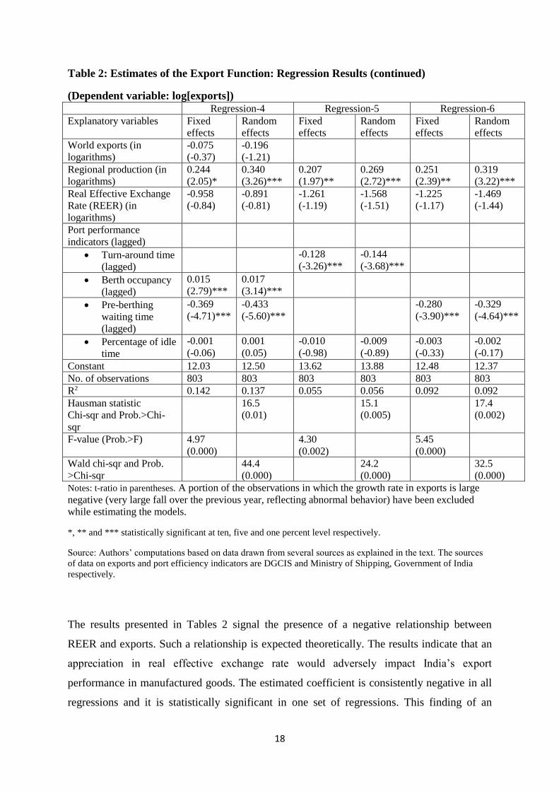
Table 2: Estimates of the Export Function: Regression Results (continued)
(Dependent variable: log[exports]) Regression-4 Regression-5 Regression-6
Explanatory variables Fixed
effects
Random
effects
Fixed
effects
Random
effects
Fixed
effects
Random
effects
World exports (in
logarithms)
-0.075
(-0.37)
-0.196
(-1.21)
Regional production (in
logarithms)
0.244
(2.05)*
0.340
(3.26)***
0.207
(1.97)**
0.269
(2.72)***
0.251
(2.39)**
0.319
(3.22)***
Real Effective Exchange
Rate (REER) (in
logarithms)
-0.958
(-0.84)
-0.891
(-0.81)
-1.261
(-1.19)
-1.568
(-1.51)
-1.225
(-1.17)
-1.469
(-1.44)
Port performance
indicators (lagged)
• Turn-around time
(lagged)
-0.128
(-3.26)***
-0.144
(-3.68)***
• Berth occupancy
(lagged)
0.015
(2.79)***
0.017
(3.14)***
• Pre-berthing
waiting time
(lagged)
-0.369
(-4.71)***
-0.433
(-5.60)***
-0.280
(-3.90)***
-0.329
(-4.64)***
• Percentage of idle
time
-0.001
(-0.06)
0.001
(0.05)
-0.010
(-0.98)
-0.009
(-0.89)
-0.003
(-0.33)
-0.002
(-0.17)
Constant 12.03 12.50 13.62 13.88 12.48 12.37
No. of observations 803 803 803 803 803 803
R2 0.142 0.137 0.055 0.056 0.092 0.092
Hausman statistic
Chi-sqr and Prob.>Chi-
sqr
16.5
(0.01)
15.1
(0.005)
17.4
(0.002)
F-value (Prob.>F) 4.97
(0.000)
4.30
(0.002)
5.45
(0.000)
Wald chi-sqr and Prob.
>Chi-sqr
44.4
(0.000)
24.2
(0.000)
32.5
(0.000)
Notes: t-ratio in parentheses. A portion of the observations in which the growth rate in exports is large
negative (very large fall over the previous year, reflecting abnormal behavior) have been excluded
while estimating the models.
*, ** and *** statistically significant at ten, five and one percent level respectively.
Source: Authors’ computations based on data drawn from several sources as explained in the text. The sources
of data on exports and port efficiency indicators are DGCIS and Ministry of Shipping, Government of India
respectively.
The results presented in Tables 2 signal the presence of a negative relationship between
REER and exports. Such a relationship is expected theoretically. The results indicate that an
appreciation in real effective exchange rate would adversely impact India’s export
performance in manufactured goods. The estimated coefficient is consistently negative in all
regressions and it is statistically significant in one set of regressions. This finding of an

19
inverse relationship between REER and export performance is in agreement with the findings
of several earlier econometric studies on determinants of India’s export (for example,
Veeramani, 2008; Kapur and Mohan, 2014; Raissi and Tulin, 2015; and Dash et al. 2018).21
From the model results, a positive relationship is found between domestic production of
manufactured goods and exports of such goods. The coefficient of regional industrial
production variable is positive in all the regression equations estimated and is statistically
significant in most of them. The results may be interpreted as indicating that a rapid growth
in domestic production of manufactured goods in a region of India will have a positive effect
on exports of manufactured goods from that region.
Two indicators of port efficiency which receive relatively greater attention in the study,
namely turn-around time and operating surplus, have been included in most regressions in
Table 2. For both of them, the estimated coefficients are found to be statistically significant at
five percent or one percent level. The coefficient of turn-around time is negative and the
coefficient of berth occupancy rate is positive (the signs of the coefficients are as expected).
Evidently, these results indicate that improved port efficiency favourably impacts export
performance. The results do not change if instead of lagged values of these indicators, the
current year values are used (ignoring the issue of possible endogeneity). This may be seen
from Annex-I (comparison of Regressions 14 and 15).
For pre-berthing waiting time, the coefficient is found to be negative, as expected. The
coefficient is statistically significant. The finding of a negative coefficient of pre-berthing
waiting time is in agreement with the finding of a negative coefficient of turn-around time.
As regards, the percentage of idle time, the coefficient is negative in most cases. It is not
found statistically significant. Yet, the results in respect of the percentage of idle time are
broadly in line with the results for other performance indicators.
Considering the results in respect of the four indicators of port efficiency presented in Table
2, it seems reasonable to infer that port efficiency matters for export competitiveness, and
improvements attained in port efficiency will help in increasing exports of manufactured
products from India. This finding of the present study is consistent with the findings of Ghosh
and De (2002) who found a positive effect of port efficiency on traffic handled in ports in
India.
21 It may be pointed out here that Bhanumurthy and Sharma (2013) did not find such a relationship between REER and India’s export performance.

20
3.3.2 Model Explaining Growth in Exports
The estimates of the model explaining growth in exports are presented in Table 3. As
mentioned earlier, the Generalized Method of Moments (GMM) has been applied to estimate
the model of export growth performance. The system GMM estimator (Arellano and Bover,
1995; Blundel and Bond, 1998) has been used.
Regressions (7) and (8) reported in Table 3 include the regional production growth variable.
These regressions follow the specification given in equation (2) above. One unsatisfactory
aspect of the model estimates is that the coefficient of the regional production growth
variable is found to be negative which is contrary to expectations and is in conflict with the
results for regional production variable in the estimates of export function presented in Table
2. Therefore, in Regression (9), the regional production growth variable has been dropped.
Regressions (7), (8) and (9) have been estimated using data for the period 2001-2014. A
change is made in Regression (10) which has been estimated using data for a shorter period,
2001-2010. The rationale for taking data for a shorter period for this model estimate is as
follows. It has been noted earlier in Section 2 that the volume index of India’s imports had a
clear upward trend during 2001-2010 and a downward trend thereafter, which was reflected
in stagnation in cargo handled in Indian ports and a marked fall in capacity utilization. This
makes the period 2011-2014 different in certain ways from the period 2001-2010, from the
viewpoint of the econometric analysis presented here. It would be useful therefore to find out
how the model estimates change if data for the period 2001-02 to 2010-11 are used rather
than 2001-02 to 2014-15. It is interesting to note from Table 3 (Regression 10) that when
data for the period 2001-2010 are used for estimating the model of export growth
performance, the coefficient of regional production growth variable is found to be positive as
expected.

21
Table 3: Estimates of the Model of Export growth Performance, System GMM
(Dependent variable: Growth rate in exports) Explanatory variable Regression-7 Regression-8 Regression-9 Regression-10
Growth rate in exports
lagged by one year
-0.158
(-1.96)*
-0.156
(-1.92)*
-0.159
(-1.86)*
-0.172
(-1.36)
Growth rate in world exports 0.335
(1.28)
0.387
(1.38)
0.320
(1.09)
0.493
(2.33)**
Growth rate in regional
production
-0.085
(-0.36)
-0.072
(-0.32)
0.403
(1.18)
Rate of change in REER -0.965
(-0.81)
-1.148
(-1.03)
-0.837
(-0.79)
-0.716
(-0.49)
Rate of change in Port
performance indicators
• Turn-around time -0.097
(-2.16)**
-0.094
(-1.36)
-0.093
(-1.98)**
• Berth occupancy 0.018
(1.68)*
0.014
(1.23)
0.017
(1.48)
0.018
(1.44)
• Pre-berthing waiting
time
-0.098
(-0.78)
• Percentage of Idle
time
-0.009
(-1.38)
-0.008
(-1.20)
-0.008
(-1.30)
-0.007
(-1.15)
Rate of growth in port
capacity
0.809
(2.64)***
0.916
(2.64)**
0.842
(2.49)**
0.623
(1.38)
Port capacity growth
interacted with Dummy
variable for low capacity
utilization rate in the
previous year
-3.629
(-1.52)
-3.478
(-1.59)
-3.877
(-1.94)*
-1.675
(-0.95)
Constant 0.010 0.000 0.001 -0.069
Data period 2001-2014 2001-14 2001-2014 2001-2010
No. of observations 719 719 719 477
No. of instruments 86 86 85 44
AR(1), z-value and prob. -3.65
(0.0003)
-3.58
(0.0003)
-3.61
(0.0003)
-3.31
(0.0009)
AR(2), z-value and prob. 0.65
(0.52)
0.69
(0.49)
0.66
(0.51)
0.79
(0.43)
Sargan test, chi-sqr and Prob.
value
60.3
(0.91)
57.7
(0.94)
58.7
(0.93)
43.5
(0.13)
Wald Chi-sqr and
Prob.>Chi-sqr
22.2
(0.008)
16.2
(0.063)
24.6
(0.002)
32.1
(0.0002)
Notes: t-ratio in parentheses. A portion of the observations in which the growth rate in exports is large
negative (very large fall over the previous year, reflecting abnormal behavior) have been excluded
while estimating the models. Regression (10) is based on data for a shorter time period. The rate of
capacity utilization during this period was relatively higher. The cut-off for defining low capacity
utilization has therefore been taken as 60% instead of the cut-off of 50% used for Regressions (7)-(9).
*, ** and *** statistically significant at ten, five and one percent level respectively.
Source: Authors’ computations based on data drawn from several sources as explained in the text. The sources
of data on exports and port capacity, utilization rate and port efficiency indicators are DGCIS and Ministry of
Shipping, Government of India respectively.
22
In the regression results reported in Table 3, the coefficient of REER is found to be negative
as expected in all the regressions but is not found statistically significant in any of them. Yet
the fact that the coefficient is consistently negative and is in the range of -0.7 to -1.1 across
the four regressions is noteworthy. Making an overall assessment, it may be said that the
results indicate a negative relationship between REER and export performance, which
corroborates the results reported in Table 2 (as well as the findings of several earlier studies
on the impact of REER on India’s exports). The implication is that an appreciation in real
effective exchange rate would have an adverse effect on manufactured exports from India.
The coefficient of the world exports variable is positive in all the regressions. It is statistically
significant in one of the regression equations estimated. Based on these results as well as the
results reported in Annex-I, and drawing additionally on the findings of some earlier studies
on export function for manufactured products from India, it seems there is basis to argue that
an increase in international demand will have a significant positive impact on manufactured
goods exports from India.
The coefficient of port capacity growth variable is positive in all four regressions and
statistically significant in three of them. The coefficient of the interaction term involving
growth rate in port capacity and dummy variable for low capacity utilization is negative in all
regressions. In one of the regression equations estimated, it is found to be statistically
significant at ten percent level. The inference that may be drawn from these results reported
in Table 3 is that a faster growth in port capacity raises the growth rate in manufactured
exports. However, for a port in which capacity utilization rate was low (less than 50%) in the
previous year, the effect of port capacity growth on export growth is relatively smaller.
Turning now to the other results reported in Table 3, it is seen from the table that the
coefficient of lagged export growth variable is consistently negative and is statistically
significant in three of the four regression equations estimated. The interpretation of these
results is that a high growth rate in exports of a particular product group through a particular
port achieved in a particular year has a base effect and tends to lower the growth rate next
year.
The coefficient of change in turn-around time is negative and that of change in berth
occupancy rate is positive. In terms of the signs of coefficients, these results match the results
reported in Table 2. While the coefficient of change in turn-around time is found to be

23
statistically significant in two regressions and the coefficient of change in berth occupancy
rate is found to be statistically significant in one of the regression equations estimated.
The coefficients of the turn-around time and berth occupancy rate, the two port efficiency
indicators which receive greater attention in this study were found to be rightly signed and
statistically significant in the estimates of the model explaining level of exports in Table 2. In
the results reported in Table 3, the coefficients are rightly signed though the level of
statistical significance is lower than that in the results reported in Table 2. Yet, it would not
be wrong to claim that the results reported in Table 3 in regard to turn-around time and berth
occupancy rate lend support to the findings emerging from the estimates presented in Table 2.
It should be realized that the relatively lower statistical significance of the coefficients of
turn-around time and berth occupancy rate in Table 3 is not altogether unexpected because a
model in which the dependent variable is in growth rate form is likely to have a weaker fit
than a model in which the dependent variable is in level form.
The coefficients of other indicators of port efficiency, namely pre-berth waiting time and
percentage of idle time match the signs of these coefficients in Table 2. Thus, there is some
degree of similarity between the results reported in Tables 2 and 3 in regard to the port
efficiency indictors. The overall assessment that can be made on the basis of the results
reported in Table 3 taken together with the results presented in Table 2 is that efficiency in
port operations has a significant positive effect on India’s exports of manufactured products.
4. Conclusion
In this paper, an attempt has been made to assess the impact of port infrastructure
development and efficiency in port operations on India’s exports of manufactured goods.
The analysis was done with the help of port-wise data on exports of six major manufactured
product categories for the period 2001-02 to 2014-15. The results of econometric analysis
brought out that improved efficiency of port operations has a positive impact on export
performance. It appears that improved port efficiency enhances competitiveness of India’s
manufactured exports enabling Indian manufacturing firms to export more.
The results of econometric analysis revealed that addition to port capacity contributes to
growth in manufactured exports. It is interesting to note that in the period since 2010-11, port
capacity in India has grown rapidly but port traffic handled has not increased leading to a fall

24
in capacity utilization in most ports. It seems that the contribution of port capacity
development to annual growth rate in manufactured exports from India during 2011-2014
was relatively lower than that during 2001-2010.
The results of econometric analysis indicate that India’s manufactured products exports are
impacted positively by global demand and negatively by appreciation in REER. These results
corroborate the findings of several earlier studies. Another important finding of the
econometric analysis is that domestic production volume bears a positive relationship with
manufactured exports. A positive relationship is found between exports of manufactured
products through a port and the production of manufactured products in the region the port is
situated.

25
References
Aksoy, M. Ataman and Helena Tang (1992), “Imports, Exports, and Industrial Performance in India,
1970-88,” Policy Research Working paper no. WPS 969, World Bank.
Arellano, Manuel, and Olympia Bover (1995), “Another look at the instrumental variable estimation
of error-components models,” Journal of econometrics 68(1): 29-51.
Behar, Alberto, Phil Manners, and Ben Nelson (2009), “Exports and Logistics.” The Department of
Economics, Oxford University Working Paper Series.
Bhanumurthy N. R. and Chandan Sharma (2013), “Does Weak Rupee Matter for India’s
Manufacturing Exports?” Working paper no. 2013-115, National Institute of Public Finance and
Policy, New Delhi.
Blundell, Richard, and Stephen Bond (1998), “Initial Conditions and Moment Restrictions in
Dynamic Panel-Data Models.” Journal of Econometrics 87 (1): 115–43.
Clark, Ximena, David Dollar, and Alejandro Micco (2004), “Port Efficiency, Maritime Transport
Costs, and Bilateral Trade,” Journal of Development Economics 75(2): 417-50.
Dash, Aruna Kumar, Subhendu Dutta, Rashmi Ranjan Paital (2018), “Bilateral Export Demand
Function of India: An Empirical Analysis,” Theoretical Economics Letters, 8: 2330-2344.
De, Prabir and Buddhadeb Ghosh (2003), “Causality between performance and traffic: an
investigation with Indian ports,” Maritime Policy and Management 30(1): 5-27.
De, Prabir (2009), Globalisation and the Changing Face of Port Infrastructure: The Indian
Perspective, Bern: Peter Lang AG.
Francis, Smitha (2015), “India’s Manufacturing Sector Export Performance during 1999-2013: A
Focus on Missing Domestic Inter-Sectoral Linkages,” Working Paper no. 182, Institute for Studies in
Industrial Development, New Delhi.
Ghosh, Buddhadeb and Prabir De (2002), “Impact of Performance Indicators and Labour Endowment
on Traffic: Empirical Evidence from Indian Ports,” International Journal of Maritime Economics
2(4): 259-82.
Goldar, Bishwnath (1989), “Determinants of India’s Export Performance in Engineering Products,
1960-79,” Developing Economies 27(1): 3-18.
Iwanow, Tomasz and Colin Kirkpatrick (2008), “Trade Facilitation and Manufactured Exports: Is
Africa Different?” World Development 37(6):1039-50.
Inoue, Takeshi (2014), “An Empirical Analysis of the Aggregate Export Demand Function in Post-
Liberalization India,” Global Economy Journal, 14(1): 79–88, DOI: https://doi.org/10.1515/gej-2013-
0013.
Kapur Muneesh and Rakesh Mohan (2014), “India’s Recent Macroeconomic Performance: An
Assessment and Way Forward” IMF Working Paper no. WP/14/68, International Monetary Fund,
Washington DC.
Nordas, H., E. Pinali, and M. Geloso Grosso (2006), “Logistics and Time as a Trade Barrier.” OECD
Trade Policy Working Paper 35. Paris: OECD.

26
Panchamukhi, V.R. (1997), “Quantitative Methods and their Applications in International
Economics,” in K.L. Krishna (ed), Econometric Applications in India, Delhi: Oxford University
Press.
Portugal-Perez, Alberto and John S. Wilson (2010), “Export Performance and Trade Facilitation
Reform Hard and Soft Infrastructure,” Policy Research Working Paper no. 5261, Development
Research Group, Trade and Integration Team, World Bank.
Raissi, Mehdi and Volodymyr Tulin (2015), “Price and Income Elasticity of Indian Exports — The
Role of Supply-Side Bottlenecks,” IMF Working Paper no. WP/15/161, Asia and Pacific Department,
International Monetary Fund, Washington DC.
Sinha, Dipendra (2001), “A Note on Trade Elasticities in Asian Countries,” International Trade
Journal, 15 (2): 221-237.
Srinivasan, T.N. (1998), “India's Export Performance: A Comparative Analysis”, in I.J. Ahluwalia
and I.M.D. Little (eds.), India's Economic Reforms and Development: Essays for Manmohan Singh,
Delhi: Oxford University Press.
Veeramani, C. (2008), “Impact of exchange rate appreciation on India’s exports,” Economic and
Political Weekly 43(22): 10-14 (May 31 – June 6).
Veeramani, C., Lakshmi A., Prachi Gupta (2017), “Intensive and Extensive Margins of Exports: What
Can India Learn from China?” Working Paper no. WP-2017-002, Indira Gandhi Institute of
Development Research, Mumbai.
Virmani, Arvind (1991) “Demand and Supply Factors in India’s Trade,” Economic and Political
Weekly 26(6): 309-14 (February 9).
Virmani, Arvind, Bishwanath Goldar, Choorikkad Veeramani and Vipul Bhatt (2004), “Impact of
tariff reforms on Indian industry: assessment based on a multi-sector econometric model, Working
paper no. 135, Indian Council for Research in International Economic Relations, New Delhi.
United Nations Conference on Trade and Development (UNCTAD) (2009), “Impact of Global
Slowdown on India’s Exports and Employment”, Report Prepared under UNCTAD-Govt.of India-
DFID Project ‘Strategies and Preparedness for Trade and Globalization in India’.

27
Annex-I: Export Function Estimates, Additional Results
Dependent variable: log[exports] Method: Fixed Effects Model
Explanatory variables Regression-
11
Regression-
12
Regression
-13
Regression-
14
Regression-
15
World exports (in
logarithms)
0.660
(2.58)**
0.659
(2.58)**
0.632
(2.48)**
Regional production
(in logarithms)
0.405
(3.20)***
0.177
(1.68)*
0.225
(2.37)**
Real Effective
Exchange Rate
(REER) (in
logarithms)
-0.967
(-0.83)
-1.337
(-1.15)
-1.035
(-0.98)
-1.243
(-1.18)
Trend -0.054
(-2.42)**
-0.045
(-1.80)*
-0.084
(-3.03)***
Port performance
indicators (lagged)
• Turn-around
time (lagged)
-0.171
(-4.01)***
• Turn-around
time (current)
-0.205
(-4.84)***
• Berth
occupancy
(lagged)
0.013
(2.49)**
• Berth
occupancy
(current)
0.014
(2.80)***
Constant 105.6 91.4 165.9 12.16 12.46
No of observations 866 866 866 803 803
R-squared 0.018 0.018 0.001 0.082 0.089
F-value (Prob.>F) 3.35(0.036) 2.47(0.061) 4.43(0.001) 5.64(0.000) 8.15(0.000)
Notes: t-ratio in parentheses. A portion of the observations in which the growth rate in exports is large
negative (very large fall over the previous year, reflecting abnormal behavior) have been excluded
while estimating the models.
*, ** and *** statistically significant at ten, five and one percent level respectively.
Source: Authors’ computations based on data drawn from several sources as explained in the text.