The Impact of Secondary Schooling in Kenya:

A Regression Discontinuity Analysis∗

Owen Ozier†

Department of EconomicsUniversity of California at Berkeley

January 17, 2011

JOB MARKET PAPER

Abstract

I estimate the impacts of secondary school on human capital, occupational choice, andfertility for young adults in Kenya. Probability of admission to government secondaryschool rises sharply at a score close to the national mean on a standardized 8th gradeexamination, permitting me to estimate causal effects of schooling in a regression dis-continuity framework. I combine administrative test score data with a recent surveyof young adults to estimate these impacts. My results show that secondary schoolingincreases human capital, as measured by performance on cognitive tests included in thesurvey. For men, I find a drop in the probability of low-skill self-employment, as well assuggestive evidence of a rise in the probability of formal employment. The opportunityto attend secondary school also reduces teen pregnancy among women.

JEL Codes: I21,J31,O12,O15

∗I am indebted to Martha Bailey, Lori Beaman, Marianne Bitler, Gustavo Bobonis, Blastus Bwire, DavidCard, Pedro Carneiro, Pascaline Dupas, Esther Duflo, Steve Fazzari, Frederico Finan, Willa Friedman,Sebastian Galiani, Justin Gallagher, Francois Gerard, Erick Gong, Joan Hamory Hicks, Jonas Hjort, GuidoImbens, Gerald Ipapa, Pamela Jakiela, Seema Jayachandran, Pat Kline, Michael Kremer, Ashley Langer,Yong Suk Lee, Karen Levy, Vikram Maheshri, Isaac Mbiti, Jamie McCasland, Justin McCrary, EdwardMiguel, Sendhil Mullainathan, Salvador Navarro, Carol Nekesa, Rohini Pande, Bruce Petersen, RobertPollak, Jim Powell, Jon Robinson, Alex Rothenberg, and Kevin Stange, as well as participants in theMidwest International Economic Development Conference, Northeast Universities Development ConsortiumConference, and seminars at UC Berkeley, for their helpful comments on this project. All errors are myown.†Please direct correspondence to ozier@econ.berkeley.edu.

1 Introduction

The expansion of schooling in sub-Saharan Africa over the last fifty years has made basic

education more accessible to many of the world’s poorest: between 1970 and 2005, average

schooling attained by young Africans rose from 2.6 years to 6.1 years, and continues to

grow.1 Increases in educational participation and attainment have coincided with rising

literacy and formal sector employment across the continent, though the direction of causal-

ity is not clear. Wage returns to education have been shown in other developing country

contexts (Duflo 2001), but similar patterns have not been demonstrated as convincingly in

Africa. One complicating factor is that rates of employment are quite low. In 2008, for

example, only 38 percent of Kenyan men were employed by someone outside their fam-

ily.2 In this context, the effects of education on human capital accumulation, occupational

choice, and fertility decisions may in fact be more socially relevant measures of the returns

to schooling than wage effects.

Most empirical studies find little evidence that African schools have positive effects on

outcomes. Two recent papers find no positive academic effects at all: Lucas and Mbiti

(2010) show that admission to higher quality secondary schools in Kenya neither raises the

probability of completing secondary school, nor increases 12th grade test scores; de Hoop

(2010) estimates that admission to a higher quality secondary school in Malawi increases

the probability of remaining enrolled in an assigned school, but has no effect on test scores.

These studies, however, only measure the change in academic performance brought about by

increases in secondary school quality. One might reasonably expect the effect of attending

attend any secondary school to differ from the effect of increased school quality. The rise in

primary school completion associated with the achievement of the Millenium Development

Goals means that a large cohort is about to reach the age of secondary schooling, which

until now has been rationed in much of sub-Saharan Africa. Despite the policy urgency of

this issue, no study to date has identified the effect of relaxing this constraint: the impact

of secondary schooling on the marginal student in the African context.3

1Source: Barro and Lee (2010), tabulation based on 33 countries in sub-Saharan Africa.2Source: DHS (2009). This includes all age groups and covers both rural areas and urban centers.3Lucas and Mbiti (2009) find that the increased school participation in Kenya brought about by the

2

In this paper, I use a regression discontinuity approach to estimate the impacts of

secondary schooling in Kenya. The discontinuity I use is based on a standardized 8th

grade test, the Kenya Certificate of Primary Education (KCPE). Probability of admission

to government secondary school rises sharply at a cutoff score close to the national mean on

the examination. I collect an administrative KCPE dataset, and combine it with a recent,

detailed survey of young adults in Kenya that includes educational attainment, along with

a number of other outcomes. With these two datasets, I use a technique from time series

econometrics to identify the structural breaks in patterns of secondary school completion,

thereby locating the test score cutoffs in Kenya’s secondary school admission policy. I

am able to confirm that the KCPE score popularly perceived to constitute “passing” the

examination is empirically the most important for boys, while a slightly lower cutoff is

more relevant for girls. This is consistent with a recent survey of local secondary school

administrators, who report lower admissions criteria for girls.

At the admissions cutoff, I find a 15 percent jump in the probability of completing high

school. This is a large effect compared to many commonly used instruments for education.

I perform relevant specification tests, and find that this effect is significant and stable across

a range of specifications, bandwidths, controls, and sample restrictions.

Students on either side of the admissions cutoff are very similar demographically, and

in a neighborhood of the test score cutoff, admission to secondary school is “as good as

randomized” (Lee 2008). This allows me to treat the rise in schooling at the admissions

cutoff as a source of exogenous variation for estimating the impact of secondary school. I find

that completing secondary school has a substantial impact on human capital accumulation,

as measured by performance on vocabulary and reasoning tests in adulthood. I estimate

a performance improvement of 0.6 standard deviations attributable to the completion of

secondary school. This is the first paper to show such positive effects of secondary schooling

in Africa.

For labor market outcomes, I consider rates of employment and low-skill self-employment.

abolition of primary school fees actually reduces average test scores, with composition effects explaining lessthan half the decline. This, however, is a very different population from those who are on the margin ofattending secondary school.

3

I find clear causal effects: for men in their mid-twenties, completing secondary school de-

creases the probability of low-skill self-employment by roughly 50 percent. There is also

suggestive evidence of a 30 percentage point increase in the probability of formal employ-

ment, though this is not significant in all specifications. The shift out of self-employment

can interpreted in the context of a model, which I outline in Section 4. It is important to

note that most self-employment in this context is not innovative entrepreneurship. Instead,

it is what Lewis (1954) refers to as “casual labour” or “petty trade;” it is the transition

away from this sector that marks economic development (Lewis 1954, p.189).

I also find that secondary schooling causes a sharp drop in the probability of teen

pregnancy. Studies of the correlation between education and fertility have emphasized on a

number of possible ramifications: human capital accumulation in the next generation, rates

of population growth, and household bargaining, for example (Strauss and Thomas 1995).

I establish a strong causal effect of secondary schooling on early fertility, opening an avenue

for further study as this population grows older. While my estimates of the effect are

relatively large, this sort of reduction is in accord with the findings of Ferre (2009) and

Duflo, Dupas, and Kremer (2010) in Kenya, as well as Baird, Chirwa, McIntosh, and Ozler

(2010) in Malawi. This contrasts with the recent work of McCrary and Royer (2011),

who find that increases in educational attainment in the US induced by age-at-school-entry

rules have no such impact; their instrument acts through a different channel on a different

subpopulation, however, partially explaining the difference in findings.

Thus, I show large effects of secondary schooling on a number of important outcomes. A

feature of this work, as compared to other recent studies on secondary schooling in Africa,

is that I estimate impacts on the marginal student who attends secondary school. As a

result, these estimates are directly interpretable as consequences of potential policy changes

that would make secondary school rationing less restrictive. The magnitude of these effects

in a population of this age suggests that permanent differences may be revealed as this

cohort grows older, opening a clear avenue for further study.

The remainder of the paper is organized as follows: Section 2 provides a description of

4

relevant facets of the Kenyan educational system, and the data I use for estimation.4 Section

3 explains the estimation strategies employed for different types of analysis. To frame the

empirical work that follows, Section 4 provides a conceptual framework for analyzing the

education and labor market decisions that young adults face in Kenya. Section 5 presents

the detailed specification checks I carry out and the results of my analysis, and Section 6

concludes.

2 Context and Data

Since 1985, the Kenyan education system has included eight years of primary schooling

and four of secondary (Eshiwani 1990, Ferre 2009). At the end of primary school, students

take a national leaving examination, the KCPE. A score of 50% or higher—currently 250

points out of 500—is considered to be a passing grade. This exam the chief determinant of

admission to secondary schools (Glewwe, Kremer, and Moulin 2009).

Those who are not admitted to any government school may choose to re-take the ex-

amination the following year, or may consider schooling in Uganda, vocational education,

or private schools with different standards. Though an official letter of admission to a

government secondary school is rare below this cutoff, it is still not guaranteed for those

above it because the number of candidates passing the KCPE may exceed the number of

spaces available in public schools (Aduda 2008, Akolo 2008). Among those who are admit-

ted to secondary school, however, many are still unable to afford tuition and assorted fees:

while primary school has been inexpensive for many years, and was made nominally “free”

in 2003, even the lowest-tier district secondary schools cost hundreds of dollars per year

during the period observed in this study.5

2.1 Data: KLPS2 surveys

This admission rule suggests a fuzzy regression discontinuity design for estimating the

impacts of secondary schooling. The primary dataset used in this study is the Kenyan

4The data appendix provides additional details on the assembly of these datasets.5Policy changes after 2008 made low-tier secondary schools considerably less expensive in Kenya.

5

Life Panel Survey (KLPS), an ongoing survey of respondents originally from Funyula and

Budalangi Divisions of Busia District, Kenya (Baird, Hamory, and Miguel 2008). The re-

spondents were sampled from the population attending grades 2 through 7 at rural primary

schools in 1998. The first round of surveying (KLPS1) was carried out from 2003 to 2005,

while the second (KLPS2) ran from 2007 to 2009, both times tracking respondents across

provincial and even national boundaries. Because the outcomes of interest occur only for

adult respondents, I mainly use the more recent round of survey data (KLPS2), treating it

as cross-sectional observation of 5,084 individuals.

The KLPS2 survey is comprehensive, including questions on education, employment,

and fertility, as well as cognitive tests. The education section includes yearly school par-

ticipation, from which secondary school completion, grade repetition, and other measures

can be constructed; it also includes self-reported KCPE scores for students who complete

primary school. The cognitive tests administered as part of the survey assess English

vocabulary and non-verbal reasoning; the labor market section includes employment and

self-employment history, including the dates and sectors of employment, as well as wages.6

In order to use a regression discontinuity design, I restrict analysis to respondents

reporting a KCPE score in the survey, which reduces sample size from N=5,084 to N=3,305,

including only pupils who complete primary school and take the KCPE. Table 1 shows

summary statistics for the restricted KLPS2 sample. The 3,305 respondents reporting

test scores have higher educational attainment, more educated parents, and lower teen

pregnancy rates than the full sample; this is to be expected, since these are the respondents

who did not drop out during primary school.

2.2 Data: test scores

While most KLPS variables are quite stable over survey rounds, self-reported KCPE scores

are not. Grade in school in 1999, for example, has a correlation of 0.95 between responses

given in KLPS1 and four years later in KLPS2, while self-reported test score has a cor-

6Non-verbal reasoning is measured using Raven’s Matrices, one of the more reliable measures of generalintelligence (Cattell 1971); the vocabulary instrument is based on the Mill Hill test, originally designed byJ. C. Raven to complement the Matrices.

6

relation closer to 0.7. The noise in test scores could pose several problems, since I use

KCPE score as the regression discontinuity running variable.7 Noise in the form of classical

measurement error for only a random subset of the data would simply reduce the power

of the regression discontinuity design. Classical measurement error in all of the data could

eliminate the discontinuity entirely.8 On the other hand, non-classical error could invalidate

the regression discontinuity design, if either mis-reporting or test repetition were driven by

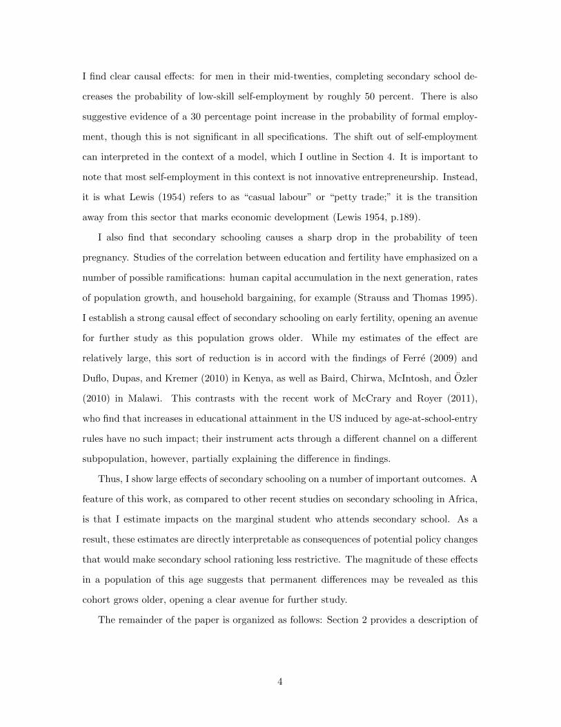
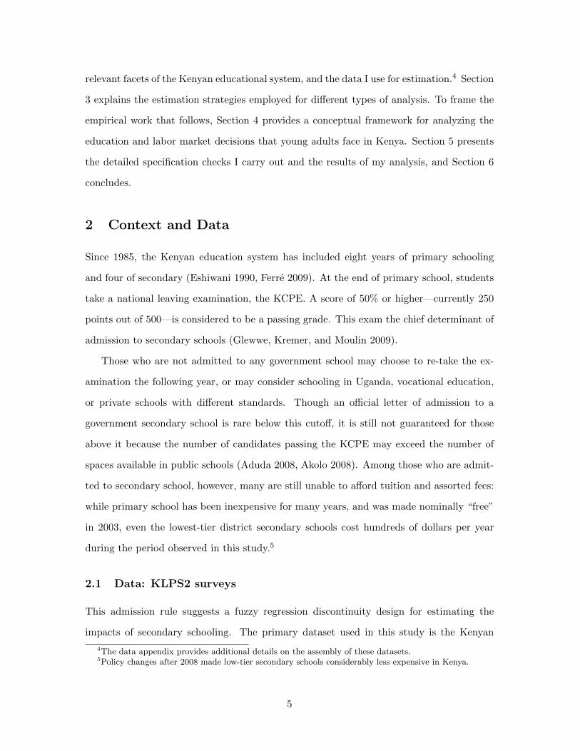
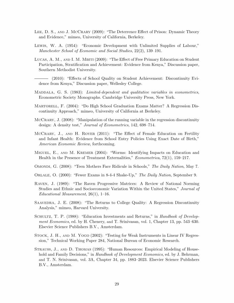
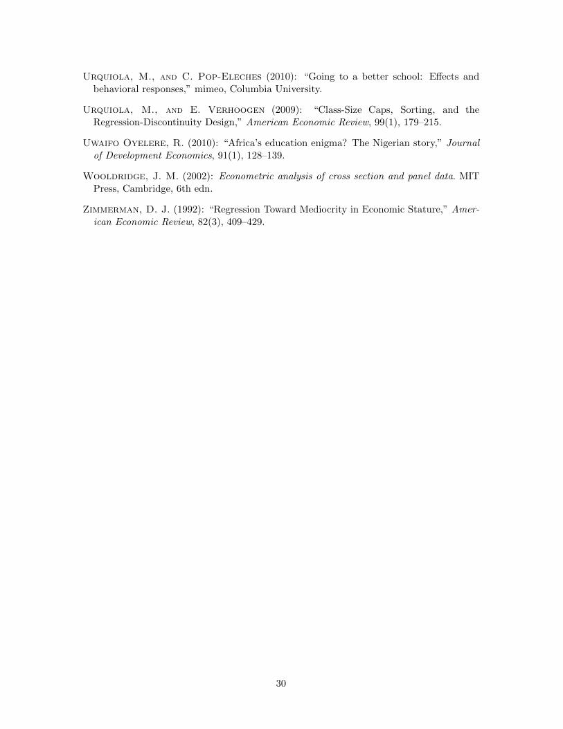
unobservables correlated with outcomes.9 A histogram of the self-reported scores, shown

in Figure 1, shows that the distribution of scores shows signs of non-classical error, in the

form of manipulation of the reported scores around the “passing” point; a test for density

smoothness proposed by McCrary (2008), shown in Figure 2, rejects at this point.

This feature of the distribution could arise simply from repeated test-taking: if many of

those who fail the test try again until they pass, the distribution of most recent test scores

will include more mass just to the right of the cutoff than to the left.10 To see whether this

phenomenon is solely responsible for the shape of the distribution, I consider a slice of the

data, available in KLPS1, in which respondents provided every test score for as many times

as they had taken the KCPE. Even if the most recent test score is endogenous with respect

to the respondent’s type and the location of the cutoff, the first test score should not be.

Appendix Figures A2 and A3 show that although the problem is less severe in this restricted

sample, even these first scores do not have a smooth density at the discontinuity. However,

administrative data on scores in the region display no such irregularity at the cutoff score,

so I conclude that the self-reports are, in many cases, incorrect, and administrative data

must be matched to the KLPS2 dataset in order to use a regression discontinuity design.11

To complement the KLPS data, I gathered an auxiliary dataset of 17,384 official KCPE

scores from District Education Offices and, when the district-level offices did not have the

records, directly from primary schools. The official records I was able to collect in 2009 and

2010 include roughly 88 percent of the PSDP schools during the years of interest in this

7Some authors, such as Imbens and Lemieux (2008), refer to this as a “forcing variable.”8More detailed discussion of these points is provided in Appendix A.2.9See Martorell (2004) for discussion of multiple potential effects of test repetition.

10See Appendix A.2 for a concrete example.11I show the distribution of regional 2008 test scores in Appendix A.4.

7

study.12 Based on name, year, and school, I am able to cross-check KCPE scores for roughly

77 percent of the KLPS respondents who report taking the KCPE. While many self-reported

scores are in accordance with the official records, there is substantial misreporting.13

Using the 88 percent coverage of the administrative data I could collect, a matching

algorithm14 is used to identify corresponding administrative records for more than 2,500

of the 3,305 respondents reporting a score. For 2,273 respondents, I find exactly one test

score; for 263 more, I find two scores in different (typically consecutive) years. Using the

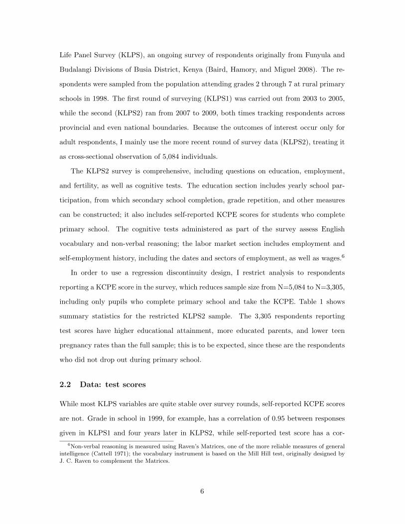
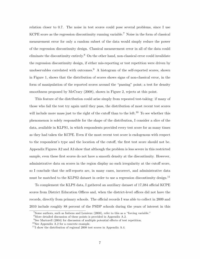
KLPS2 survey to determine whether matched scores are first or second attempts, I am able

to clearly identify 2,167 first test scores.15 Their distribution is plotted in Figure 3 and is

tested for a density break in Figure 4. I find no evidence of manipulation of administratively

reported first test scores.

2.3 Gender-specific discontinuities

The KCPE cutoff for secondary school admission is well-known in Kenya; national media

recently reported that “Out of the over 695,000 candidates who sat the KCPE examina-

tion, 350,000 candidates attained over 250 marks, making them eligible to join secondary

school.”16 However, a survey of secondary schools in the area suggests that, though 250 is

the modal 2009 cutoff score reported by school administrators, many competitive schools

use higher cutoffs.17 Further, many schools report different cutoffs for boys and girls: seven

out of eighteen reporting cutoff scores for girls report a value below 250. As such, 250 may

not be the cutoff where the largest fraction of girls are exogenously induced to attend sec-

ondary schools.18 To address these, I apply a technique from the structural break literature,

following Card, Mas, and Rothstein (2008): I first restrict attention to a window of scores

12Every PSDP school with missing records was visited at least once by me or another member of the datacollection team; recent re-districting and political upheaval in Kenya, combined with local problems withrecord storage over the last 12 years, prevented the collection of the last 12 percent.

13I discuss the matching process and characterize misreporting in Appendix section A.1.5.14The procedure is described in Appendix A.1.5.15For some cases where I observer only one test score, it either appears to be a second score, or it is

unclear whether it is a first or second score. I exclude these when using only first test score.16Excerpted from Akolo (2008).17Edward Miguel and Matthew Jukes, unpublished data (2009).18Because the recent survey only included 2009 cutoffs, I re-visited secondary schools to find out their

history of admissions rules, but current school administrations were not able to provide records of admissionsrules covering the period of study in this paper.

8

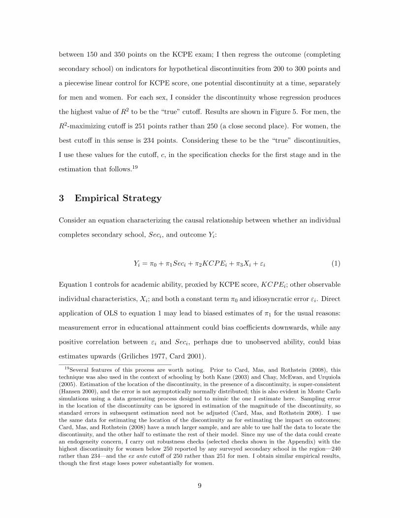
between 150 and 350 points on the KCPE exam; I then regress the outcome (completing

secondary school) on indicators for hypothetical discontinuities from 200 to 300 points and

a piecewise linear control for KCPE score, one potential discontinuity at a time, separately

for men and women. For each sex, I consider the discontinuity whose regression produces

the highest value of R2 to be the “true” cutoff. Results are shown in Figure 5. For men, the

R2-maximizing cutoff is 251 points rather than 250 (a close second place). For women, the

best cutoff in this sense is 234 points. Considering these to be the “true” discontinuities,

I use these values for the cutoff, c, in the specification checks for the first stage and in the

estimation that follows.19

3 Empirical Strategy

Consider an equation characterizing the causal relationship between whether an individual

completes secondary school, Seci, and outcome Yi:

Yi = π0 + π1Seci + π2KCPEi + π3Xi + εi (1)

Equation 1 controls for academic ability, proxied by KCPE score, KCPEi; other observable

individual characteristics, Xi; and both a constant term π0 and idiosyncratic error εi. Direct

application of OLS to equation 1 may lead to biased estimates of π1 for the usual reasons:

measurement error in educational attainment could bias coefficients downwards, while any

positive correlation between εi and Seci, perhaps due to unobserved ability, could bias

estimates upwards (Griliches 1977, Card 2001).

19Several features of this process are worth noting. Prior to Card, Mas, and Rothstein (2008), thistechnique was also used in the context of schooling by both Kane (2003) and Chay, McEwan, and Urquiola(2005). Estimation of the location of the discontinuity, in the presence of a discontinuity, is super-consistent(Hansen 2000), and the error is not asymptotically normally distributed; this is also evident in Monte Carlosimulations using a data generating process designed to mimic the one I estimate here. Sampling errorin the location of the discontinuity can be ignored in estimation of the magnitude of the discontinuity, sostandard errors in subsequent estimation need not be adjusted (Card, Mas, and Rothstein 2008). I usethe same data for estimating the location of the discontinuity as for estimating the impact on outcomes;Card, Mas, and Rothstein (2008) have a much larger sample, and are able to use half the data to locate thediscontinuity, and the other half to estimate the rest of their model. Since my use of the data could createan endogeneity concern, I carry out robustness checks (selected checks shown in the Appendix) with thehighest discontinuity for women below 250 reported by any surveyed secondary school in the region—240rather than 234—and the ex ante cutoff of 250 rather than 251 for men. I obtain similar empirical results,though the first stage loses power substantially for women.

9

Instead, I use a regression discontinuity approach to identify the effect of secondary

school on outcomes. As described in Section 2, Kenyan students who take the primary

school leaving examination (KCPE) face an admission rule: below a cutoff score, ci, it is

more difficult to gain admission to secondary school. The identifying assumptions in my

analysis are that all other outcome-determining characteristics except for the probability

of secondary school attendance vary smoothly near the cutoff, and that outcomes change

at the cutoff only because of the induced change in schooling. Because the probability

of attendance does not jump from zero to one, this is a “fuzzy” regression discontinuity

(Imbens and Lemieux 2008), so the causal effect of secondary school on outcomes is:

τFRD =limk↓ci E[Y |KCPE = k]− limk↑ci E[Y |KCPE = k]

limk↓ci E[Sec|KCPE = k]− limk↑ci E[Sec|KCPE = k](2)

As long as the order of polynomial in the running variable and the data window are the

same for the first and second stage outcomes, estimation of τFRD in equation 2 is equivalent

to an instrumental variables approach, where the first and second stages are:

Seci = α0 + α1Abovei + α2Ki + α3Ki ·Abovei + α4Xi + ζi (2a)

Yi = β0 + βFRDSeci + β2Ki + β3Ki ·Abovei + β4Xi + ξi (2b)

In equations 2a and 2b, I use normalized KCPE scores, Ki = KCPEi − ci, shifted so

that the discontinuity occurs at Ki = 0; the variable Abovei is equal to 1 if Ki ≥ 0,

and 0 otherwise; the parameter of interest is βFRD; I allow the relationship between Yi

and Ki to have different slopes on either side of the discontinuity. This is an estimation

based on compliers, the population who would not complete secondary school if they had

scored below the cutoff, but who would if they score above it. The estimated effect is a

local average treatment effect at the point in the test score distribution where the cutoff

falls. By definition, it is the policy-relevant cutoff for a policy change that would consider

moving the cutoff slightly and changing the number of available slots in secondary schools.

In this case, however, the cutoff also falls very near the median (and mean) of the test score

10

distribution, which suggests that the effects I measure are relevant for the median Kenyan

KCPE-taker, rather than for outliers in the education or skill distribution.20

3.1 Other estimation approaches using the same identification

In the case of binary outcome variables, such as whether a respondent is pregnant by age 18,

a nonlinear instrumental variables approach may be appropriate. In particular, I consider

the IV probit, with the same first stage given in equation 2a, but with second stage:

Pr [Preg18i = 1] = Φ(γ0 + γFRDSeci + γ2Ki + γ3Ki ·Abovei + γ4Xi

)(3)

The IV probit estimation procedure is only correctly specified when the first stage residuals

are asymptotically normally distributed, and when the first stage is linear.21 An alternative,

when the first stage outcome is binary, is the (recursive) bivariate probit proposed by

Maddala (1983):22

Seci = 1 (δ0 + δ1Abovei + δ2Ki + δ3Ki ·Abovei + δ4Xi + τi > 0) (4)

Yi = 1 (φ0 + φ1Seci + φ2Ki + φ3Ki ·Abovei + φ4Xi + ωi > 0) (5)

This approach uses Seci rather than Seci in the second stage, because it explicitly models

endogeneity through the correlation, ρ, between τi and ωi. Though Maddala does not

specify any particular cumulative distribution function, I follow Greene (2007), Evans and

Schwab (1995), and others in imposing a bivariate normal distribution on the error terms:

τi

ωi

∼ N 0

0

, 1 ρ

ρ 1

(6)

Though in practice, IV probit and bivariate probit yield marginal effects estimates that are

20By contrast, many US studies relying on date-of-birth identification strategies are focused on relativelylow-achieving students; studies such as the work of Saavedra (2008) in Colombia estimate the returns onlyto the highest-quality universities. Neither class of coefficient is necessarily relevant for the bulk of thepopulation.

21A binary endogenous regressor would typically not yield asymptotically normal residuals.22Maddala (1983) presents the model on pp. 122-3; Greene (2007) discusses the model further on pp.823-6;

Wooldridge (2002) also discusses it on p.478.

11

often quite similar to those given by 2SLS, they have the advantage that, when correctly

specified, they can provide greater statistical power when the probability of an outcome

variable is very close to either zero or one.23 The cost of this power is additional distribu-

tional assumptions, however, so I present results from each of these estimation techniques,

when appropriate.

4 Conceptual Framework

Much of the empirical work relating educational attainment to labor market decisions has

focused on wage in contexts with relatively high employment levels. Employment outside

the family is low in Kenya, and lower in this region and at the age of KLPS2 respondents.

For this section, I focus only on male respondents. According to the DHS (2009), while 38

percent of Kenyan men were employed by someone outside their family, only 29 percent of

the 20-25 year-old men in rural Nyanza Province (adjoining the KLPS2 study region) were

employed. For the oldest two cohorts of men in KLPS2 (with a mean age of 24.8 years),

that figure is 32 percent. Even those who have found jobs took, on average, several years to

find them. As the DHS (2009) data illustrate, this is an age at which young men who did

not attend secondary school have had much longer to find jobs than those who did attend,

but those who did attend are about to overtake them in terms of employment rates. This is

analogous to the crossover point in developed-country labor markets. Either before finding

outside employment, or instead of it, young men may immediately take up low-intensity

farming on family land, or may start low-capital-intensity, low-skill self-employment, such

as operating a bicycle taxi. Here, I outline a simple, stylized model relating educational

attainment and labor market decisions in this setting.

In the model, agents face a series of decisions. The first is whether to obtain secondary

schooling, conditional on costs. The second is how to approach the labor market after

schooling: whether to search for a formal sector job or not, and whether to do so while

either self-employed or farming. The third decision arrives only if the agent chose to search

for a formal sector job; once a job offer appears, the agent may either take the job or reject

23This can be shown in Monte Carlo simulations, for example.

12

it, and if he rejects it, he may either continue self-employment or farming, or may switch

between self-employment and farming.

First, agents i choose whether to undertake secondary schooling in the face of costs that

are discontinuous at the KCPE cutoff; the cost of secondary school is lower if the agent

passes: csecpass < csecfail. The prices include the opportunity cost and financial cost of repeating

eighth grade. I denote the choice to complete secondary school edi = 1; otherwise, edi = 0.

Additional schooling causes an increase in human capital, θi: θ1i = θ0

i + β · edi.

After schooling, agents can be self-employed, or be farmers. Which is better depends

on the relative profitability of self-employment and farming, represented here as potential

wages, max(wselfi , wfarmi ), which vary across the population. For simplicity, I assume that

everyone who is not otherwise employed is farming, though this may not take many hours

because, at this age, agents are generally helping out on their parents’ farms rather than

farming their own plots. Self-employment and farming may be undertaken as soon as an

agent chooses, but formal employment requires search; I model the search for employment

as a geometric arrival process with probability q of success in each period. Self employment

depends more on labor than does farming, however, so at the same cost of searching for a

job in each period, cu, the expected time to job arrival is greater for the self-employed than

for farmers: τ s = 1/qs > τ f = 1/qf ⇐⇒ qs < qf .

The notion that self-employment depends more on labor than does farming finds empir-

ical support in the KLPS2 data. Self-employed men report working 40 hours in the past

week; this is both the median and approximately the mean. Men who whose only work

is farming reported working an average of 14 hours in the previous week (with a median

of 12 hours).24 The model imposes the restriction that the expected time to job arrival is

greater for the self-employed than for farmers. If this is true, and arrivals are a geometric

process, then the amount of time between the end of school and the start of formal sector

employment–among those who find formal employment–should be longer for those who start

in self-employment than for those who start in farming. Cross-sectional regressions showing

this pattern are shown in Appendix Table A1; in each case, self-employment is associated

24Both the average self-employment and farming hours are tabulated conditional on positive hours in eachactivity; unconditional results are similar.

13

with a job search that is between 0.6 and 1.0 years longer than without self-employment

(and thus, implicitly, with farming).

Wages from employment are unknown to agents prior to the arrival of a job offer, but the

wage is fixed once the offer arrives. In advance, however, agents do know the distribution of

wages conditional on their human capital. Assume wage offers are lognormal, parameterized

by geometric mean µ(θ1i ). I assume that µ is increasing in θ. This is validated empirically

by a simple regression of the natural logarithm of wages on the standardized human capital

measure at survey time, in the subpopulation reporting a wage. Several cross-sectional

regressions showing this pattern are shown in Appendix Table A2; the coefficient is always

positive and significant.

Conditional on a job offer with wage wempi , agents will either take the outside op-

tion wri = max(wfarmi , wselfi ) or take the job; the latter occurs with probability pi =

Prob[wempi > wri ], and has expected wage value Ewemp>wr

i = E[wempi |wempi > wri ]. If the

job search is successful in a particular period, then search ends with a permanent wage

whose expected value is Ewbesti = pi ·Ewemp>wr

i +(1−pi)wri . With a discount rate of δ and

infinite periods, expected value of the best non-search option is simply U r = wri /(1 − δ).

The expected value of searching while farming is:

EUfs =

(wfarmi − cu +

qfδ

1− δ· Ewbesti

)+ (1− qf )δ · EUfs

EUfs =1

1− δ + qfδ·(wfarmi − cu +

qfδ

1− δEwbesti

)

The expected value of searching while self-employed, likewise, is:

EU ss =1

1− δ + qsδ·(wselfi − cu +

qsδ

1− δEwbesti

)

Conditional on human capital θ1i , risk-neutral agents choose the option with the highest

expected payoff:

max(U r, EUfs, EU ss

)Hence, agents will choose to search for a job when max

(EUfs, EU ss

)> U r, and choose to

14

attend secondary school when:

max((EUfs, EU ss

)|edi = 1

)− cseci > max

((U r, EUfs, EU ss

)|edi = 0

)

4.1 Some implications of this framework

Lemma 1. EU ss and EUfs are increasing in q, the probability of finding a job in each

period. (See Appendix Section A.3 for proof.)

Implication 1. wfarmi ≥ wselfi =⇒ EUfs > EU ss: If, for a particular agent, the effective

wage from farming (weakly) exceeds that from self-employment, then the expected utility

from searching for a job while farming must exceed the expected utility from searching for

a job while self-employed.

Proof. Given that wfarmi ≥ wselfi , substituting into the equations for EUfs and EU ss, and

relying on the assumption that qf > qs, the result follows from Lemma 1.

Implication 2. wfarmi < wselfi =⇒ Pr[EUfs > EU ss] is weakly increasing in µ: If, for a

particular agent, the effective wage from farming is lower than that from self-employment,

then the probability that expected utility from searching for a job while farming exceeds that

from searching for a job while self-employed is (weakly) increasing in the geometric mean

of wage offers. (See Appendix Section A.3 for proof.)

Implication 3. Pr[EUfs > EU ss] is weakly increasing in θ1i , human capital.

Proof. The result follows immediately from the assumption that µ(θ1i ) is an increasing

function, and Implications 1 and 2.

Implication 3 suggests a test for reduced self-employment at the discontinuity, which I

discuss further in the next Section.

15

5 Results

5.1 Specification: bandwidth and polynomial order

For the first stage, I consider a window of data symmetric about the discontinuity, and

regress completion of secondary school on an indicator for scoring above the discontinuity

and piecewise linear controls in test score. I plot the resulting estimates of the disconti-

nuity magnitude in Figure 6, as a function of the width of the data window; here, I scale

down scores by a factor of 100 so that coefficient estimates in subsequent tables are read

more easily. The discontinuity estimate fluctuates slightly, but remains significant and of

similar magnitude no matter which bandwidth I use.25 At each bandwidth, I carry out a

specification test in which in addition to the discontinuity dummy and the piecewise linear

controls, I include indicators for narrow-width bins of KCPE scores: 251-260, 261-270, et

cetera.26 I test these indicators for joint significance; if they are significant, I consider the

piecewise linear first stage to be mis-specified. This test rejects for widths of 90 points

and higher on either side of the discontinuity. The same is true when I include a piecewise

quadratic control in test score. Thus, for the rest of this paper, I use a bandwidth of 80

points on either side of the discontinuity.27 Finally, I use Akaike’s information criterion to

confirm that the first-order polynomial control is sufficient: piecewise linear (as opposed

to constant, quadratic, cubic, or quartic) is the “best” specification according to AIC for

both the 80-point bandwidth and nearly all other bandwidths under consideration. I use

the same bandwidth and order of polynomial (linear) in both the first and second stage

estimation, so that I can simply use 2SLS both for estimation and standard errors.28

I carry out validity tests of the smoothness assumption using observables, four of which

are depicted graphically in Figure 7. Gender, age, and mother’s and father’s education vary

25Here I use the term bandwidth in the sense of Imbens and Lemieux (2008), Lee and Lemieux (2010), andothers in the regression discontinuity literature to mean the window of data used for estimation; this is nota non-parametric regression; I do not weight data differently according to distance from the discontinuity.

26For this test, I follow Lee and Lemieux (2010) and Lee and McCrary (2009). The results are similarwhen I vary bin width, for example using a width selected by a leave-one-out cross-validation procedure.

27Alternatively, I can use the procedure suggested by Imbens and Kalyanaraman (2009); this yieldssimilar “optimal” bandwidths for most outcomes, though smaller bandwidths for a few. Results are largelyunchanged.

28 See, in particular, Lee and Lemieux (2010) Section 4.3.3.

16

smoothly at the boundary, with differences that are neither large enough to be important

nor statistically significant. This contrasts with Urquiola and Verhoogen (2009), who show

that schools’ responses to a class-size policy discontinuity in Chile can invalidate a regression

discontinuity research design. While they find large and significant differences in parents’

education levels at the discontinuity (as well as sharp changes in the class size histogram

near cutoffs), I find no such patterns here.29

5.2 First stage: discontinuity

The first stage discontinuity is shown in the upper-left pane of Figure 8, and in a regression

framework in Table 2.30 In Table 2, the discontinuity is estimated first with genders pooled

(columns 1-3), then separately among men (columns 4-6) and women (columns 7-9). I

show the results with and without a piecewise quadratic control and controls for other

covariates: age, gender, parents’ education levels, and cohort dummies. I cannot reject

that the discontinuities for men and women are of the same magnitude, though the smaller

point estimate for women is consistent with the lower overall level of secondary schooling

for women in this setting. My preferred specifications are given in columns (2), (5), and (8),

in which the discontinuity is measured as a 16-percentage-point change in the probability

of completing secondary school for men; a 13 percent change for women, and a 15 percent

change when pooled.31 That controls do not substantially change the point estimate is

unsurprising, given that they do not change significantly at the discontinuity.

When the estimation is carried out separately by gender, the discontinuity is significant

for both men and women, but the F-statistic is now below the rule of thumb for weak

29See Section A.1.5 and Figure 4. In particular, while I cannot rule out all types of cheating on the KCPE,as in the Texas testing context investigated by Martorell (2004), none of the known mechanisms for cheatingon the exam would permit endogenous sorting around the discontinuity.

30In this case, because the data window constrains predictions to within the unit interval, a logit orprobit specification yields marginal effects that are almost identical in magnitude and significance to thediscontinuity estimated here in a linear probability model.

31Decomposition as suggested by Gelbach (2009) shows that the change in coefficient magnitude fromcolumn (7) to column (9) is mostly due to the inclusion of the covariate controls; the slightly larger standarderror is brought about because of the inclusion of the piecewise quadratic in the running variable. A separateissue is that small fraction of the sample is still in school; this fraction varies slightly at the discontinuity,and as such, the completion of secondary schooling may be viewed as a censored outcome in the first stage,which could be the source of some bias. In practice, restricting the sample to respondents who are surveyedat least five years after they take the KCPE does not substantially alter the results.

17

instruments for the subsample of women (Stock and Yogo 2002)—though I cannot reject

the equality of the discontinuities for men and women. However, because the model is

just-identified, the weak-instruments bias towards OLS is not present (Angrist and Pischke

2009), though tests may not be correctly sized. In contrast, Uwaifo Oyelere (2010) finds

that variation in free primary education in Nigeria predicts years of education equally well

for men and women. This could be because free primary school induces additional schooling

at too young an age for womens’ early marriage and fertility decisions to be relevant, and

would have been especially true in the period when Nigeria’s primary education system was

first coming into existence, included in Uwaifo Oyelere’s (2010) analysis.

In Figure 9, I show the estimated difference between the cumulative distribution func-

tions for education of the populations on either side of the discontinuity. For each point in

Figure 9, I estimate a separate regression of the probability that respondents attain more

than x years of education on a piecewise linear control and an indicator for the disconti-

nuity; the plot shows the coefficients and confidence intervals on the discontinuity for each

of these outcomes. The KCPE discontinuity as an instrument clearly predicts secondary

schooling, and moreover, secondary school completion. The estimates, however, drop to

insignificance when estimating the probability of attaining more than 12 years of schooling:

the KCPE score that induces a marginal student to attending and complete seondary school

does not induce the student to attend college.

5.3 Estimation of outcomes

5.3.1 Human capital

I begin with analysis of the impact of schooling on human capital. The KLPS2 survey in-

cludes a commonly used test of cognitive ability—a subset of Raven’s Progressive Matrices—

and an English-language vocabulary test based on the Mill Hill synonyms test. Adaptations

of both measures have been used internationally for several decades, and each captures dif-

ferent aspects of intelligence.32 I standardize both outcomes so that they are measured

32Though standardized to have mean zero and standard deviation one in the population, in Table 1these two cognitive measures have positive mean and standard deviations slightly less than one, becausethese summary statistics are only shown for the sample with a restricted range of first KCPE scores. The

18

in terms of standard deviations in the KLPS2 population, and show both OLS and 2SLS

results for a combined Z-score33 and separately by test in Panel A of Table 3: completing

secondary school improves performance on these tests by 0.6 standard deviations, with very

similar estimates given by 2SLS and (potentially biased) OLS. This estimate is robust to

the inclusion of controls (column 4), and when decomposed, is driven by the larger and

more precisely estimated effect in vocabulary. The reduced form effect, roughly 0.1 stan-

dard deviations at the discontinuity, is shown in the upper right panel of Figure 8. To

the extent that subsequent outcomes depend on a mixture of human capital and signaling,

this is evidence that secondary schooling in Kenya does not play a purely signaling role:

students gain measurably from schooling.34

These results contrast with the recent work of Lucas and Mbiti (2010), who show that

increased quality of secondary schooling (at higher discontinuities in KCPE score) has no

impact on subsequent academic outcomes. This appears to be true even when the marginal

student admitted into the school is not the worst student in the higher-quality school. A

clue to reconciling their findings with mine may lie in the recent work of Urquiola and

Pop-Eleches (2010). Using a similar multiple-discontinuity design to estimate the returns

to secondary school quality in Romania, they find very modest positive effects, around

.04 standard deviations on an academic test. These effects are simply too small to be

detectable in the Lucas and Mbiti (2010) study, and when compared with the results I

show in Table 3, it is clear that attending any secondary school has a much larger effect

than increasing the quality of the secondary school. de Hoop (2010) also finds no positive

effects of secondary school quality on a standardized test outcome in Malawi, but this

“Matrices” are often considered to measure something akin to “fluid” intelligence, while the vocabulary testmeasures something more related to what specialists in the field call “crystallized” intelligence (Cattell 1971).The relationship of the two measures appears similar here to in other settings: in these data, as elsewhere(Raven 1989), their correlation is near 0.5.

33The combined Z-score is equivalent to the “mean effect” of Kling, Liebman, and Katz (2007) when nodata are unevenly missing and the estimation procedure is the same for both.

34A pessimistic interpretation might hypothesize that the longer respondents have been out of school, theworse they perform on tests; since secondary schooling delays exit from school, the apparent positive effectis simply a delayed deterioration of human capital. The data do not support such an interpretation: thelonger respondents have been out of school (and thus the older they are), the better they do on the testsadministered during KLPS2; the coefficient is too small (around 0.02 standard deviations per additionalyear out of school) to explain an effect more than an order of magnitude larger; and the effect remainssignificant and of the same magnitude in both OLS and 2SLS after controlling for duration out of school.

19

is in keeping with the aforementioned studies. On the other hand, the Lucas and Mbiti

(2009) finding that increased primary schooling actually reduced average performance on

the KCPE exam is driven by the setting: the universal primary education policy they study

couples an increase in years of schooling with increased enrollment. While test scores might

have risen for some students who received more schooling, Lucas and Mbiti (2009) note that

the class size and compositional changes overwhelm any positive effect on test scores.

5.3.2 Self-employment and employment

Next, I examine the impact of education on labor market outcomes. Because many of

the younger respondents are still in school, and because men are typically primary earners

in Kenya, I consider only the oldest two cohorts of men for this analysis, so that the

incapacitation effect of continued schooling does not dominate the patterns of interest.35

According to 2008 Demographic and Health Survey (DHS) data, young men in Kenya

without secondary school have a higher employment rate at age 20 than do men who

complete secondary school, since the latter group has had less time to look for jobs. At

roughly age 25 (the mean age of the older two male KLPS2 cohorts), DHS data show

roughly equal employment rates in these two groups; as they grow older still, the better

educated are more likely to be employed. I confirm exactly this pattern in KLPS2, shown in

Table 4, columns 1 and 2. OLS shows a fairly precise zero effect of secondary schooling on

employment at this age. However, the regression discontinuity approach gives very different

results: the coefficient on schooling is positive and significant depending on controls, shown

in IV probit and bivariate probit specifications in columns 3-6. While 2SLS is positively

signed, it is insignificant; this is in part because 2SLS is less efficient than estimation via IV

probit and bivariate probit when the true model is nonlinear and the mean of the response

variable is close to zero or one, as in this case.36 Depending on the specification, I find a

rise in employment of between 24 and 43 percent in response to secondary schooling.

35As shown in Panel C of Table 1, only 13 percent of the men in the oldest two cohorts are still in school,as compared to 44 percent in the younger four cohorts. Human capital effects of secondary school remainbroadly similar when limiting the sample to respondents who were in standards 6 and 7 in 1998, thoughstandard errors widen (predictably) with the lower sample size; results shown in Panel B of Table 3.

36As a diagnostic, predicted values from 2SLS clearly lie outside the unit interval.

20

Besides being employed by someone outside their family, many respondents are self-

employed. Of these, 88 percent have no employees: common self-employment occupations

in KLPS2 include fishing, hawking assorted wares, and working as a “boda-boda” bicycle

taxi driver. On the other hand, among the employed respondents, the degree of skill varies

among unskilled (loader of goods onto vehicles), semi-skilled (factory worker, carpenter,

mechanic), and high-skill professional occupations (electronics repair, teachers, and other

government and NGO employees).

As in other labor market studies of relatively young men (Griliches 1977, Zimmerman

1992), I use sector of employment rather than wage to estimate the impact of secondary

schooling. Clear patterns emerge when I measure the effect of education on (implicitly low-

skill) self-employment, shown as a reduced form graph in the lower left panel of Figure 8, and

presented in the second row of Table 4. While secondary education and self-employment are

negatively associated in the cross-section (columns 1 and 2), the causal impact of secondary

schooling on low-skill self-employment is much larger; marginal effects from IV probit and

bivariate probit estimation are in broad agreement with the 2SLS coefficients: a 40-50

percent lower probability of being self-employed among those who go to secondary school

because they pass the KCPE cutoff. This tests one of the predictions of the framework

outlined in Section 4, in particular Implication 3: young men should be less likely to take

up low-skill self-employment if they hope to be able to obtain a better job. Table 4 shows

that indeed, they are.

5.3.3 Fertility

While labor market outcomes are of interest for the men in this sample, fertility and health

outcomes are of more importance for the women: women are less than half as likely to be

employed as men in each of the six KLPS2 cohorts.37

In a reduced form graph, shown in in the lower right panel of Figure 8, and in Table 5,

I look at the probability of pregnancy by age 18 among female KLPS2 respondents. The

37At the discontinuity, men appear slightly less likely to be married by survey time, and women appearslightly more likely to be married, but neither effect is significant. Conditional on marriage, spouse educationrises slightly at the discontinuity (as one might expect), but this effect is also statistically insignificant (resultsnot shown).

21

association between secondary schooling and decreased early fertility is strong: in the last

two columns, OLS shows a roughly twelve percentage point drop in teen pregnancy among

secondary school finishers. While these are only cross-sectional associations, their sign

agrees with associations seen in the U.S., Taiwan, and Colombia, summarized by Schultz

(1988). Two-stage least squares predicts outside the unit interval, since again, this is a

low-probability outcome, so I use IV probit and bivariate probit estimation in the first four

columns and find a near elimination of teen pregnancy among compliers at the discontinuity,

robust to the inclusion of the usual controls.

This finding contrasts with the work of McCrary and Royer (2011), who find no con-

clusive effect of education on timing of womens’ first births. As McCrary and Royer (2011)

point out, however, their study is based on a manipulation of the age at school entry rather

than the age at school exit, as is the case here. In effect, when a girl starts school one year

earlier than her counterparts because her birthday falls before a cutoff date, she has one

more year of education by the time she considers dropping out of school at a particular

age, perhaps in relation to the legal minimum. Their date-of-birth instrument thus pre-

dicts educational attainment among those who, for the most part, do not go on to tertiary

schooling and in fact stop schooling almost as soon as possible. However, if pregnancy in

the McCrary and Royer (2011) population is timed in relation to age rather than school-

ing, such variation in educational attainment would have no effect. In my case, however,

young teens are given or denied the opportunity to continue schooling (thus varying age

at exit) at the KCPE discontinuity. The KCPE discontinuity only has an effect on those

who choose to continue beyond primary education (delaying school exit), and who must

be considering tradeoffs between continuing their education and raising a family. These

may be higher ability students, relative to the Kenyan distribution, than are the McCrary

and Royer (2011) respondents in relation to the US distribution. Thus, while they find

essentially no impact of education on early fertility using variation in age at school entry,

it may still be sensible that in contrast to their work, I find large effects.

Other studies in sub-Saharan Africa have found similar, though smaller, effects of school-

ing on teen pregnancy. Ferre (2009) finds that a policy shift reclassifying 8th grade from

22

secondary to primary school increased the fraction of students reaching 8th grade, thereby

reducing teen pregnancy by 10 percentage points in Kenya in the 1980s. Duflo, Dupas,

and Kremer (2010) observe a 1.5 percentage point reduction in teen childbearing in Kenya

in response to a school uniform distribution program that helped girls stay in school; and

Baird, Chirwa, McIntosh, and Ozler (2010) find that a conditional cash transfer to bring

dropouts back into school reduces teen pregnancies by 5 percentage points in Malawi.

Since many of the secondary schools are single-sex, one interpretation could be that

teens in secondary school simply see members of the opposite sex less frequently than they

otherwise would, so lower rates of pregnancy follow. This interpretation is not supported

by the data, though: when I categorize secondary schools as single-sex or mixed, I see no

significant difference in the pregnancy decline across the two types of schools.38

In Kenya, dropping out of school is more common among girls than boys, and is most

pronounced once girls enter their teens (Kremer, Miguel, and Thornton 2009). This is

closely linked to pregnancy: girls in the Kenyan schools are “required to discontinue their

studies for at least a year39” if they become pregnant. Schooling and childbearing in Kenya

are in practice nearly mutually exclusive, as is true in many other contexts (Field and

Ambrus 2008). Though I am aware of no rule prohibiting teen mothers from returning to

school—though rules of that sort exist in other sub-Saharan countries (Ferre 2009)—teen

mothers still face stigmatization in Kenyan primary and secondary schools (Omondi 2008),

so even after giving birth, they are unlikely to continue their schooling. The practical mutual

exclusivity of pregnancy and schooling means that high-ability girls at the discontinuity face

a tradeoff between attending secondary school and starting a family immediately; this policy

may also differ from the policy environment in the US.

5.4 Interpretation of the discontinuity

Though the probability of secondary schooling changes sharply at that point, covariates do

not. If the probability of non-government secondary schooling changed at the discontinuity,

38In the cross section, the reductions in teen pregnancy associated with going to the two types of schoolsare also similar and statistically indistinguishable: 9 percentage points for girls at mixed schools, and 10percentage points for those who attend all-girls’ schools.

39Excerpted from Ferre (2009), p. 5.

23

however, it could be interpreted differently. For example, in order to attend secondary

school without attaining the cutoff score, students may choose to enroll in secondary school

in Uganda, rather than Kenya. Less than five percent of the sampled respondents attend

secondary school in Uganda, however, and at the discontinuity, there appears to be no jump

in the probability of attending secondary school in Uganda.40

The discontinuity may also be interpreted as an increase in years of schooling rather than

an increase in the probability of secondary school completion. This version of the first stage

is shown in Appendix Table A3. This first stage is evident in all the same specifications as

before, and the coefficient magnitudes are roughly four times larger, since the indicator for

completing secondary school represented four years of schooling. Appendix Tables A4, A5,

and A6 show the results under this first stage, and for the most part, the coefficients are

simply four times smaller. This interpretation is misleading, however: while compliers at

the discontinuity do gain approximately 0.16 standard deviations on the cognitive tests for

each additional year of schooling (Appendix Table A4, columns 3 and 4), this is true because

nearly all the compliers at the discontinuity gain exactly 4 years of schooling (Figure 9),

and thus just above 0.6 standard deviations on the tests (Table 3, columns 3 and 4). The

relevant policy experiment is not to extend secondary school by an additional year, but

to change the cutoff so that a larger fraction of the population attends—and completes—

secondary school. Nevertheless, results are largely robust to the alternative specification.

6 Conclusion and Future Work

Secondary schooling in Kenya has large effects on human capital, reducing low-skill self em-

ployment, increasing formal employment, and with suggestive evidence of reducing the job

search time after school. Teen pregnancy is dramatically reduced by secondary schooling,

and I find suggestive evidence of a similarly marked decline in child mortality.

The discontinuity occurs at the most policy-relevant position, near the mean score on the

national primary school leaving examination: perhaps as externally valid as a single “fuzzy”

40The lack of a jump at the discontinuity is robust to the controls used throughout this paper; the pointestimate is usually positive and between 0.005 and 0.013, but statistically indistinguishable from zero; resultsnot shown.

24

discontinuity could be. An expansion of secondary schooling that preserved the quality of

secondary schools but reduced the minimum required score would be likely to bring about

the effects I esimate on roughly 15 percent of the population near the discontinuity: the

compliers. As governments including Kenya’s consider the expansion of secondary schooling

against other policy options, this study should provide a useful guidepost for understanding

the consequences of such an expansion, as long as the expansion does not substantially alter

the characteristics of the schools.

The difference between the unambiguously positive human capital findings in this pa-

per and the less cheery conclusions from other studies of education in Kenya suggest that

increased school enrollment in sub-Saharan Africa will have varying consequences, depend-

ing on how it is undertaken. The findings in this paper, and in other experimental and

quasi-experimental papers, are contingent on the nature of the exogenous variation: the

secondary school admission instrument I use, at the KCPE discontinuity, induces both a rise

in secondary school completion, and a resulting delay in pregnancy among female compliers;

a date-of-birth instrument in the US that also induces additional secondary education has

no such effect, however, both because of the timing of the education effects and because of

the underlying skills and preferences of compliers with the different instruments.

OLS and 2SLS do not always produce similarly signed effects in this analysis: cross-

sectional analysis does not reveal the impact of secondary schooling on employment on this

age, but in a causal framework, the pattern emerges. The KLPS2 cohorts are still relatively

young for employment and fertility outcomes, but a third round of KLPS surveying is

currently being planned, in which the same regression discontinuity strategy employed here

may be used to study consequences of secondary schooling once more of the respondents

have participated more extensively in marriage and labor markets. The panel nature of

the dataset will then be more useful, with multiple employment spells observed for a larger

fraction of the respondents, for example. The reduction in early fertility reported in this

paper may have benefits for the health of children in the next generation; the next KLPS

round may also be able to measure some of those effects.

This study also highlights a possible avenue for researchers interested in the conse-

25

quences of education throughout sub-Saharan Africa: many countries have examinations

much like the KCPE, with analogous cutoff rules for secondary school admission. An im-

portant caveat is that while some survey data show a very high degree of reliability, this

cannot be said for KCPE scores. Combining administrative test data with a rich follow-

up survey overcomes this obstacle, and may yield novel findings establishing causal links

between education, fertility, and labor markets throughout the developing world.

26

References

Aduda, D. (2008): “Girls Shine in KCPE,” The Daily Nation, December 30.

Ajayi, K. (2010): “Welfare Implications of Constrained Secondary School Choice inGhana,” mimeo, University of California, Berkeley.

Akolo, J. (2008): “KCPE results indicate highest gender parity,” Kenya BroadcastingCorporation, Online: http://www.kbc.co.ke/story.asp?ID=54707, Accessed on May31, 2009.

Angrist, J. D., and J.-S. Pischke (2009): Mostly Harmless Econometrics. PrincetonUniversity Press, Princeton.

Baird, S., E. Chirwa, C. McIntosh, and B. Ozler (2010): “The Short-Term Impactsof a Schooling Conditional Cash Transfer Program on the Sexual Behavior of YoungWomen,” Health Economics, 19(S1), 55–68.

Baird, S., J. Hamory, and E. Miguel (2008): “Tracking, Attrition and Data Quality inthe Kenyan Life Panel Survey Round 1 (KLPS-1),” Working Paper C08-151, Center forInternational and Development Economics Research, University of California at Berkeley.

Barro, R. J., and J.-W. Lee (2010): “A New Data Set of Educational Attainment inthe World, 1950-2010,” Working Paper 15902, National Bureau of Economic Research.

Card, D. (2001): “Estimating the Return to Schooling: Progress on Some PersistentEconometric Problems,” Econometrica, 69(5), 1127–1160.

Card, D., A. Mas, and J. Rothstein (2008): “Tipping and the dynamics of segrega-tion,” Quarterly Journal of Economics, 123(1), 177–218.

Cattell, R. B. (1971): Abilities: Their Structure, Growth, and Action. Houghton MifflinCompany, Boston.

Chay, K. Y., P. J. McEwan, and M. Urquiola (2005): “The Central Role of Noise inEvaluating Interventions That Use Test Scores to Rank Schools,” American EconomicReview, 95(4), 1237–1258.

de Hoop, J. (2010): “Selective Secondary Education and School Participation in Sub-Saharan Africa: Evidence from Malawi,” Discussion Paper TI 2010-041/2, TinbergenInstitute.

DHS (2009): Kenya Demographic and Health Survey. ICF Macro, Calverton, Maryland.

Duflo, E. (2001): “Schooling and Labor Market Consequences of School Construction inIndonesia: Evidence from an Unusual Policy Experiment,” American Economic Review,91(4), 795–813.

Duflo, E., P. Dupas, and M. Kremer (2010): “Education and Fertility: ExperimentalEvidence from Kenya,” mimeo, Massachusetts Institute of Technology.

Eshiwani, G. S. (1990): “Implementing Educational Policies in Kenya,” Africa TechnicalDepartment Series Discussion Paper 85, The World Bank.

27

Evans, W. N., and R. M. Schwab (1995): “Finishing High School and Starting College:Do Catholic Schools Make a Difference?,” Quarterly Journal of Economics, 110(4), 941–974.

Fan, J. (1992): “Design-adaptive Nonparametric Regression,” Journal of the AmericanStatistical Association, 87(420), 998–1004.

Ferre, C. (2009): “Age at First Child: Does Education Delay Fertility Timing? The Caseof Kenya,” Policy Research Working Paper 4833, The World Bank.

Field, E., and A. Ambrus (2008): “Early Marriage, Age of Menarche, and FemaleSchooling Attainment in Bangladesh,” Journal of Political Economy, 116(5), 881–930.

Gelbach, J. (2009): “When Do Covariates Matter? And Which Ones, and How Much?,”mimeo, University of Arizona.

Glewwe, P., M. Kremer, and S. Moulin (2009): “Many Children Left Behind? Text-books and Test Scores in Kenya.,” American Economic Journal: Applied Economics,1(1), 112–135.

Greene, W. H. (2007): Econometric Analysis. Prentice Hall, Upper Saddle River, 6thedn.

Griliches, Z. (1977): “Estimating the Returns to Schooling: Some Econometric Prob-lems,” Econometrica, 45(1), 1–22.

Hahn, J., P. Todd, and W. Van der Klaauw (2001): “Identification and Estimationof Treatment Effects with a Regression-Discontinuity Design,” Econometrica, 69(1), 201–209.

Hansen, B. E. (2000): “Sample Splitting and Threshold Estimation,” Econometrica,68(3), 575–603.

Imbens, G., and K. Kalyanaraman (2009): “Optimal Bandwidth Choice for the Re-gression Discontinuity Estimator,” mimeo, Harvard University.

Imbens, G. W., and T. Lemieux (2008): “Regression discontinuity designs: A guide topractice,” Journal of Econometrics, 142(2), 615–635.

Kane, T. J. (2003): “A Quasi-Experimental Estimate of the Impact of Financial Aid onCollege-Going,” Working Paper 9703, National Bureau of Economic Research.

Kling, J. R., J. B. Liebman, and L. F. Katz (2007): “Experimental Analysis of Neigh-borhood Effects,” Econometrica, 75(1), 83–119.

Kremer, M., E. Miguel, and R. Thornton (2009): “Incentives to Learn,” Review ofEconomics and Statistics, 91(3), 437–456.

Lee, D. S. (2008): “Randomized experiments from non-random selection in U.S. Houseelections,” Journal of Econometrics, 142(2), 675–697.

Lee, D. S., and T. Lemieux (2010): “Regression Discontinuity Designs in Economics,”Journal of Economic Literature, 48(2), 281–355.

28

Lee, D. S., and J. McCrary (2009): “The Deterrence Effect of Prison: Dynamic Theoryand Evidence,” mimeo, University of California, Berkeley.

Lewis, W. A. (1954): “Economic Development with Unlimited Supplies of Labour,”Manchester School of Economic and Social Studies, 22(2), 139–191.

Lucas, A. M., and I. M. Mbiti (2009): “The Effect of Free Primary Education on StudentParticipation, Stratification and Achievement: Evidence from Kenya,” Discussion paper,Southern Methodist University.

(2010): “Effects of School Quality on Student Achievement: Discontinuity Evi-dence from Kenya,” Discussion paper, Wellesley College.

Maddala, G. S. (1983): Limited-dependent and qualitative variables in econometrics,Econometric Society Monographs. Cambridge University Press, New York.

Martorell, F. (2004): “Do High School Graduation Exams Matter? A Regression Dis-continuity Approach,” mimeo, University of California at Berkeley.

McCrary, J. (2008): “Manipulation of the running variable in the regression discontinuitydesign: A density test,” Journal of Econometrics, 142, 698–714.

McCrary, J., and H. Royer (2011): “The Effect of Female Education on Fertilityand Infant Health: Evidence from School Entry Policies Using Exact Date of Birth,”American Economic Review, forthcoming.

Miguel, E., and M. Kremer (2004): “Worms: Identifying Impacts on Education andHealth in the Presence of Treatment Externalities,” Econometrica, 72(1), 159–217.

Omondi, G. (2008): “Teen Mothers Face Ridicule in Schools,” The Daily Nation, May 7.

Orlale, O. (2000): “Fewer Exams in 8-4-4 Shake-Up,” The Daily Nation, September 9.

Raven, J. (1989): “The Raven Progressive Matrices: A Review of National NormingStudies and Ethnic and Socioeconomic Variation Within the United States,” Journal ofEducational Measurement, 26(1), 1–16.

Saavedra, J. E. (2008): “The Returns to College Quality: A Regression DiscontinuityAnalysis,” mimeo, Harvard University.

Schultz, T. P. (1988): “Education Investments and Returns,” in Handbook of Develop-ment Economics, ed. by H. Chenery, and T. Srinivasan, vol. 1, Chapter 13, pp. 543–630.Elsevier Science Publishers B.V., Amsterdam.

Stock, J. H., and M. Yogo (2002): “Testing for Weak Instruments in Linear IV Regres-sion,” Technical Working Paper 284, National Bureau of Economic Research.

Strauss, J., and D. Thomas (1995): “Human Resources: Empirical Modeling of House-hold and Family Decisions,” in Handbook of Development Economics, ed. by J. Behrman,and T. N. Srinivasan, vol. 3A, Chapter 34, pp. 1883–2023. Elsevier Science PublishersB.V., Amsterdam.

29

Urquiola, M., and C. Pop-Eleches (2010): “Going to a better school: Effects andbehavioral responses,” mimeo, Columbia University.

Urquiola, M., and E. Verhoogen (2009): “Class-Size Caps, Sorting, and theRegression-Discontinuity Design,” American Economic Review, 99(1), 179–215.

Uwaifo Oyelere, R. (2010): “Africa’s education enigma? The Nigerian story,” Journalof Development Economics, 91(1), 128–139.

Wooldridge, J. M. (2002): Econometric analysis of cross section and panel data. MITPress, Cambridge, 6th edn.

Zimmerman, D. J. (1992): “Regression Toward Mediocrity in Economic Stature,” Amer-ican Economic Review, 82(3), 409–429.

30

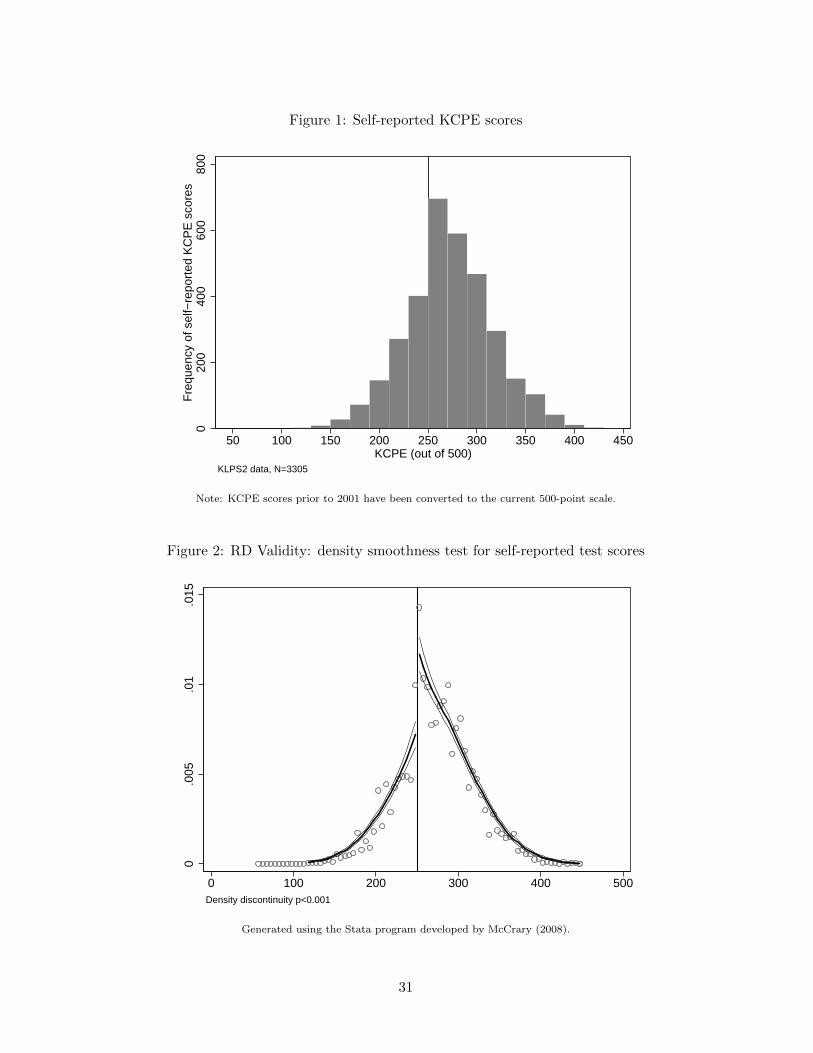
Figure 1: Self-reported KCPE scores

020

040

060

080

0F

requ

ency

of s

elf−

repo

rted

KC

PE

sco

res

50 100 150 200 250 300 350 400 450KCPE (out of 500)

KLPS2 data, N=3305

Note: KCPE scores prior to 2001 have been converted to the current 500-point scale.

Figure 2: RD Validity: density smoothness test for self-reported test scores

0.0

05.0

1.0

15

0 100 200 300 400 500Density discontinuity p<0.001

Generated using the Stata program developed by McCrary (2008).

31

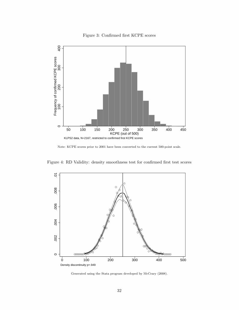
Figure 3: Confirmed first KCPE scores

010

020

030

040

0F

requ

ency

of c

onfir

med

KC

PE

sco

res

50 100 150 200 250 300 350 400 450KCPE (out of 500)

KLPS2 data, N=2167, restricted to confirmed first KCPE scores

Note: KCPE scores prior to 2001 have been converted to the current 500-point scale.

Figure 4: RD Validity: density smoothness test for confirmed first test scores

0.0

02.0

04.0

06.0

08.0

1

0 100 200 300 400 500Density discontinuity p=.949

Generated using the Stata program developed by McCrary (2008).

32

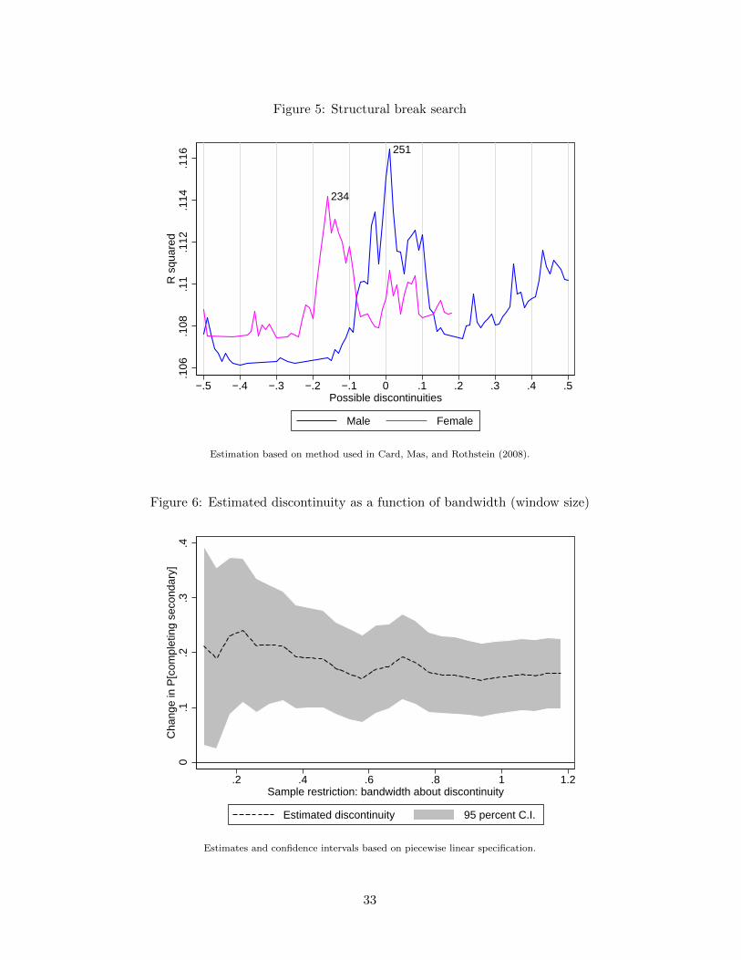
Figure 5: Structural break search

251

234.1

06.1

08.1

1.1

12.1

14.1

16R

squ

ared

−.5 −.4 −.3 −.2 −.1 0 .1 .2 .3 .4 .5Possible discontinuities

Male Female

Estimation based on method used in Card, Mas, and Rothstein (2008).

Figure 6: Estimated discontinuity as a function of bandwidth (window size)

0.1

.2.3

.4C

hang

e in

P[c

ompl

etin

g se

cond

ary]

.2 .4 .6 .8 1 1.2Sample restriction: bandwidth about discontinuity

Estimated discontinuity 95 percent C.I.

Estimates and confidence intervals based on piecewise linear specification.

33

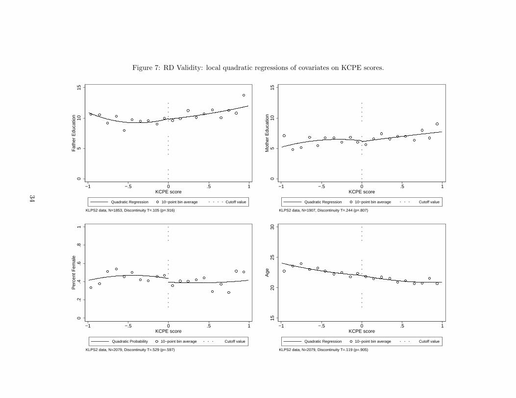
Figure 7: RD Validity: local quadratic regressions of covariates on KCPE scores.

05

1015

Fat

her

Edu

catio

n

−1 −.5 0 .5 1KCPE score

Quadratic Regression 10−point bin average Cutoff value

KLPS2 data, N=1853, Discontinuity T=.105 (p=.916)

05

1015

Mot

her

Edu

catio

n

−1 −.5 0 .5 1KCPE score

Quadratic Regression 10−point bin average Cutoff value

KLPS2 data, N=1907, Discontinuity T=.244 (p=.807)

0.2

.4.6

.81

Per

cent

Fem

ale

−1 −.5 0 .5 1KCPE score

Quadratic Probability 10−point bin average Cutoff value

KLPS2 data, N=2079, Discontinuity T=.529 (p=.597)

1520

2530

Age

−1 −.5 0 .5 1KCPE score

Quadratic Regression 10−point bin average Cutoff value

KLPS2 data, N=2079, Discontinuity T=.119 (p=.905)

34

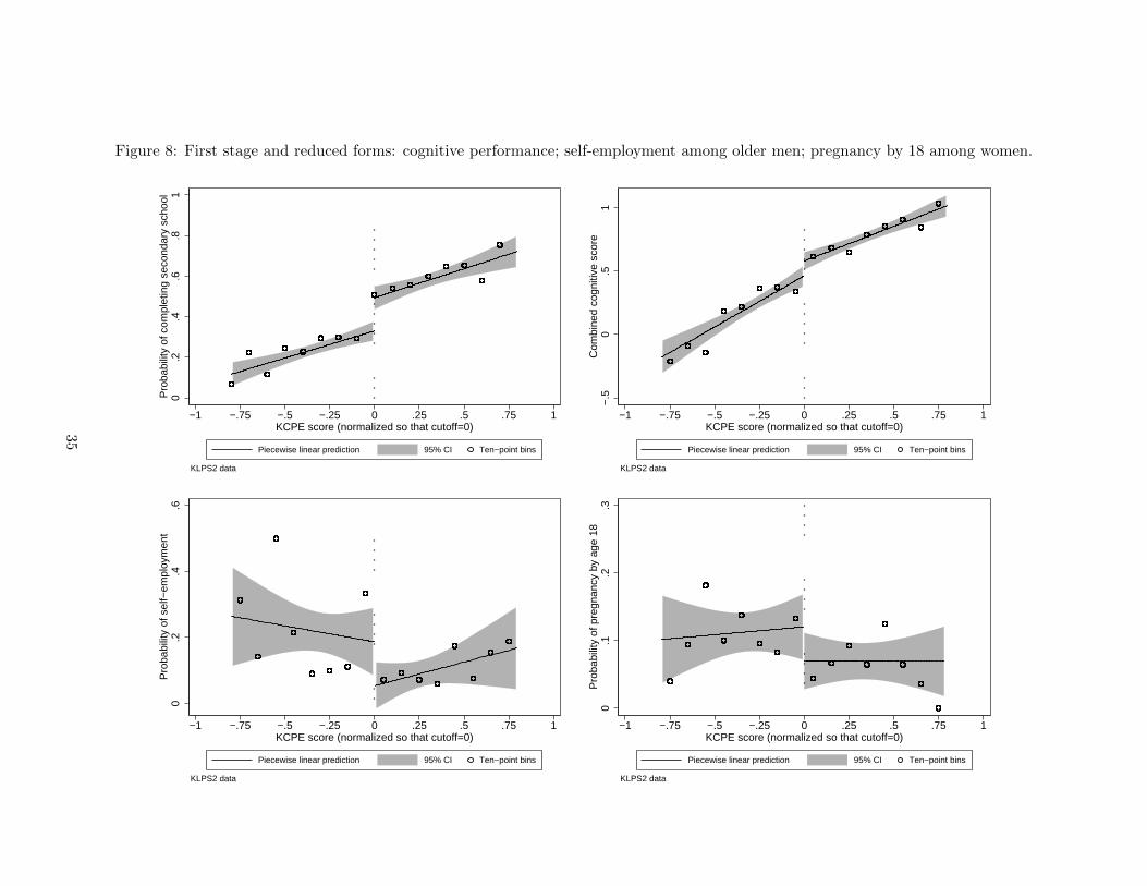
Figure 8: First stage and reduced forms: cognitive performance; self-employment among older men; pregnancy by 18 among women.

0.2

.4.6

.81

Pro

babi

lity

of c

ompl

etin

g se

cond

ary

scho

ol

−1 −.75 −.5 −.25 0 .25 .5 .75 1KCPE score (normalized so that cutoff=0)

Piecewise linear prediction 95% CI Ten−point bins

KLPS2 data

−.5

0.5

1C

ombi

ned

cogn

itive

sco

re

−1 −.75 −.5 −.25 0 .25 .5 .75 1KCPE score (normalized so that cutoff=0)

Piecewise linear prediction 95% CI Ten−point bins

KLPS2 data

0.2

.4.6

Pro

babi

lity

of s

elf−

empl

oym

ent

−1 −.75 −.5 −.25 0 .25 .5 .75 1KCPE score (normalized so that cutoff=0)

Piecewise linear prediction 95% CI Ten−point bins

KLPS2 data

0.1

.2.3

Pro

babi

lity

of p

regn

ancy

by

age

18

−1 −.75 −.5 −.25 0 .25 .5 .75 1KCPE score (normalized so that cutoff=0)

Piecewise linear prediction 95% CI Ten−point bins

KLPS2 data

35

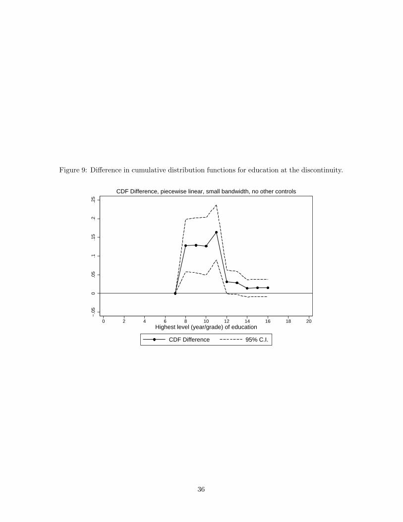
Figure 9: Difference in cumulative distribution functions for education at the discontinuity.

−.0

50

.05

.1.1

5.2

.25

0 2 4 6 8 10 12 14 16 18 20Highest level (year/grade) of education

CDF Difference 95% C.I.

CDF Difference, piecewise linear, small bandwidth, no other controls

36

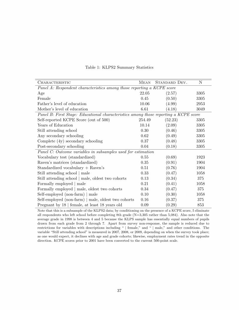
Table 1: KLPS2 Summary Statistics

Characteristic Mean Standard Dev. N

Panel A: Respondent characteristics among those reporting a KCPE scoreAge 22.05 (2.57) 3305Female 0.45 (0.50) 3305Father’s level of education 10.06 (4.99) 2953Mother’s level of education 6.61 (4.18) 3049

Panel B: First Stage: Educational characteristics among those reporting a KCPE scoreSelf-reported KCPE Score (out of 500) 254.49 (52.23) 3305Years of Education 10.14 (2.09) 3305Still attending school 0.30 (0.46) 3305Any secondary schooling 0.62 (0.49) 3305Complete (4y) secondary schooling 0.37 (0.48) 3305Post-secondary schooling 0.04 (0.18) 3305

Panel C: Outcome variables in subsamples used for estimationVocabulary test (standardized) 0.55 (0.69) 1923Raven’s matrices (standardized) 0.35 (0.91) 1904Standardized vocabulary + Raven’s 0.51 (0.76) 1904Still attending school | male 0.33 (0.47) 1058Still attending school | male, oldest two cohorts 0.13 (0.34) 375Formally employed | male 0.21 (0.41) 1058Formally employed | male, oldest two cohorts 0.34 (0.47) 375Self-employed (non-farm) | male 0.10 (0.30) 1058Self-employed (non-farm) | male, oldest two cohorts 0.16 (0.37) 375Pregnant by 18 | female, at least 18 years old 0.09 (0.29) 853

Note that this is a subsample of the KLPS2 data; by conditioning on the presence of a KCPE score, I eliminateall respondents who left school before completing 8th grade (N=3,305 rather than 5,084). Also note that theaverage grade in 1998 is between 4 and 5 because the KLPS sample has essentially equal numbers of pupilsdrawn from each grade from 2 through 7. Apart from survey non-response, the sample is reduced due torestrictions for variables with descriptions including “ | female,” and “ | male,” and other conditions. Thevariable “Still attending school” is measured in 2007, 2008, or 2009, depending on when the survey took place;as one would expect, it declines with age and grade cohorts; likewise, employment rates trend in the oppositedirection. KCPE scores prior to 2001 have been converted to the current 500-point scale.

37

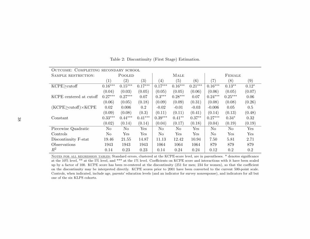
Table 2: Discontinuity (First Stage) Estimation.

Outcome: Completing secondary schoolSample restriction: Pooled Male Female

(1) (2) (3) (4) (5) (6) (7) (8) (9)

KCPE≥cutoff 0.16∗∗∗ 0.15∗∗∗ 0.17∗∗∗ 0.17∗∗∗ 0.16∗∗∗ 0.21∗∗∗ 0.16∗∗∗ 0.13∗∗ 0.12∗

(0.04) (0.03) (0.05) (0.05) (0.05) (0.06) (0.06) (0.05) (0.07)KCPE centered at cutoff 0.27∗∗∗ 0.27∗∗∗ 0.07 0.3∗∗∗ 0.28∗∗∗ 0.07 0.24∗∗∗ 0.25∗∗∗ 0.06

(0.06) (0.05) (0.18) (0.09) (0.09) (0.31) (0.08) (0.08) (0.26)(KCPE≥cutoff)×KCPE 0.02 0.006 0.2 -0.02 -0.01 -0.03 -0.006 0.05 0.5

(0.09) (0.08) (0.3) (0.11) (0.11) (0.41) (0.14) (0.13) (0.48)Constant 0.33∗∗∗ 0.44∗∗∗ 0.41∗∗∗ 0.39∗∗∗ 0.41∗∗ 0.37∗∗ 0.27∗∗∗ 0.34∗ 0.32

(0.02) (0.14) (0.14) (0.04) (0.17) (0.18) (0.04) (0.19) (0.19)

Piecewise Quadratic No No Yes No No Yes No No YesControls No Yes Yes No Yes Yes No Yes YesDiscontinuity F-stat 19.46 21.55 14.87 11.13 12.42 10.94 7.50 5.81 2.71Observations 1943 1943 1943 1064 1064 1064 879 879 879R2 0.14 0.23 0.23 0.14 0.24 0.24 0.12 0.2 0.2

Notes for all regression tables: Standard errors, clustered at the KCPE-score level, are in parentheses. * denotes significanceat the 10% level, ** at the 5% level, and *** at the 1% level. Coefficients on KCPE score and interactions with it have been scaledup by a factor of 100. KCPE score has been re-centered at the discontinuity (251 for men; 234 for women), so that the coefficienton the discontinuity may be interpreted directly. KCPE scores prior to 2001 have been converted to the current 500-point scale.Controls, when indicated, include age, parents’ education levels (and an indicator for survey nonresponse), and indicators for all butone of the six KLPS cohorts.

38

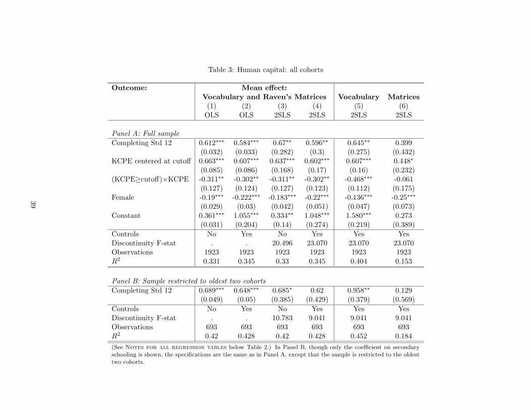
Table 3: Human capital: all cohorts

Outcome: Mean effect:Vocabulary and Raven’s Matrices Vocabulary Matrices

(1) (2) (3) (4) (5) (6)OLS OLS 2SLS 2SLS 2SLS 2SLS

Panel A: Full sample

Completing Std 12 0.612∗∗∗ 0.584∗∗∗ 0.67∗∗ 0.596∗∗ 0.645∗∗ 0.399(0.032) (0.033) (0.282) (0.3) (0.275) (0.432)

KCPE centered at cutoff 0.663∗∗∗ 0.607∗∗∗ 0.637∗∗∗ 0.602∗∗∗ 0.607∗∗∗ 0.448∗

(0.085) (0.086) (0.168) (0.17) (0.16) (0.232)(KCPE≥cutoff)×KCPE -0.311∗∗ -0.302∗∗ -0.311∗∗ -0.302∗∗ -0.468∗∗∗ -0.061

(0.127) (0.124) (0.127) (0.123) (0.112) (0.175)Female -0.19∗∗∗ -0.222∗∗∗ -0.183∗∗∗ -0.22∗∗∗ -0.136∗∗∗ -0.25∗∗∗

(0.029) (0.03) (0.042) (0.051) (0.047) (0.073)Constant 0.361∗∗∗ 1.055∗∗∗ 0.334∗∗ 1.048∗∗∗ 1.580∗∗∗ 0.273

(0.031) (0.204) (0.14) (0.274) (0.219) (0.389)

Controls No Yes No Yes Yes YesDiscontinuity F-stat . . 20.496 23.070 23.070 23.070Observations 1923 1923 1923 1923 1923 1923R2 0.331 0.345 0.33 0.345 0.404 0.153

Panel B: Sample restricted to oldest two cohorts

Completing Std 12 0.689∗∗∗ 0.648∗∗∗ 0.685∗ 0.62 0.958∗∗ 0.129(0.049) (0.05) (0.385) (0.429) (0.379) (0.569)

Controls No Yes No Yes Yes YesDiscontinuity F-stat . . 10.783 9.041 9.041 9.041Observations 693 693 693 693 693 693R2 0.42 0.428 0.42 0.428 0.452 0.184

(See Notes for all regression tables below Table 2.) In Panel B, though only the coefficient on secondaryschooling is shown, the specifications are the same as in Panel A, except that the sample is restricted to the oldesttwo cohorts.

39

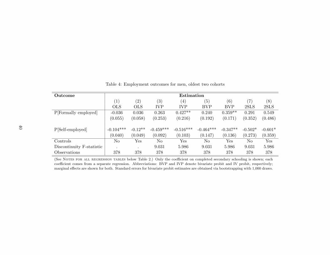
Table 4: Employment outcomes for men, oldest two cohorts

Outcome Estimation(1) (2) (3) (4) (5) (6) (7) (8)

OLS OLS IVP IVP BVP BVP 2SLS 2SLS

P[Formally employed] -0.036 0.036 0.263 0.427** 0.240 0.359** 0.291 0.549(0.055) (0.058) (0.253) (0.216) (0.192) (0.171) (0.352) (0.486)

P[Self-employed] -0.104*** -0.12** -0.459*** -0.516*** -0.464*** -0.347** -0.502* -0.601*(0.040) (0.049) (0.092) (0.103) (0.147) (0.136) (0.273) (0.359)

Controls No Yes No Yes No Yes No YesDiscontinuity F-statistic . . 9.031 5.986 9.031 5.986 9.031 5.986Observations 378 378 378 378 378 378 378 378

(See Notes for all regression tables below Table 2.) Only the coefficient on completed secondary schooling is shown; eachcoefficient comes from a separate regression. Abbreviations: BVP and IVP denote bivariate probit and IV probit, respectively;marginal effects are shown for both. Standard errors for bivariate probit estimates are obtained via bootstrapping with 1,000 draws.

40

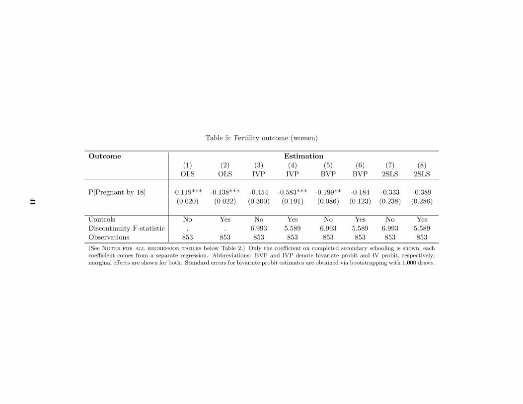
Table 5: Fertility outcome (women)

Outcome Estimation(1) (2) (3) (4) (5) (6) (7) (8)

OLS OLS IVP IVP BVP BVP 2SLS 2SLS

P[Pregnant by 18] -0.119*** -0.138*** -0.454 -0.583*** -0.199** -0.184 -0.333 -0.389(0.020) (0.022) (0.300) (0.191) (0.086) (0.123) (0.238) (0.286)

Controls No Yes No Yes No Yes No YesDiscontinuity F-statistic . . 6.993 5.589 6.993 5.589 6.993 5.589Observations 853 853 853 853 853 853 853 853

(See Notes for all regression tables below Table 2.) Only the coefficient on completed secondary schooling is shown; eachcoefficient comes from a separate regression. Abbreviations: BVP and IVP denote bivariate probit and IV probit, respectively;marginal effects are shown for both. Standard errors for bivariate probit estimates are obtained via bootstrapping with 1,000 draws.

41

A Appendix

A.1 Data

A.1.1 KCPE logistics

When students take the exam,41 they indicate a list of secondary schools they would preferto attend, including one or two from each of three tiers of secondary schools: national,provincial, and district.42 National schools are the most competitive and are considered tobe of the highest quality; district schools, the least so.

Initial admission cutoffs are determined centrally by the Ministry of Education. Thecufoffs may differ for boys and girls, and vary according to characteristics of each secondaryschool.43 After the cutoffs are decided and test results are available, heads of secondaryschools meet in groups to determine matches between schools and students, and makeadmission offers. Following this initial selection round, a variety of additional selectionmechanisms are employed: students may accept offers; students may contact other schoolswhich they would prefer to attend, to see whether the admissions committee is willing toaccept them;44 and school leaders may meet again to carry out a second round of selectionif an insufficient number of students accept offers in the first round. Nevertheless, the oddsof secondary school admission jump up sharply at a KCPE score of 250, and continue torise thereafter, as does the quality of the school to which a student is admitted.

A.1.2 KCPE scoring

From 1985 to 2000, the KCPE covered seven subjects, each scored on a 100-point scale:English, Swahili, math, science, geography, arts, and business; from 2001 onward, thelast two of these—arts and business—were removed (Orlale 2000, Kremer, Miguel, andThornton 2009). As a consequence, the KLPS data include observations in which themaximum score is 700, and observations where the maximum is 500. Throughout thispaper, I normalize all scores to the 500-point scale.

Those who are not admitted to any government school have several options if they wishto continue their education: they may repeat eighth grade and re-take the KCPE; they maystill have access to private secondary schools and vocational schools; or they may travel toUganda to enroll in school there.

A.1.3 Re-taking the KCPE

One clear pattern both from the survey data and the administrative records is that studentssometimes re-take the test. In the 2003-2005 round of surveying (KLPS1), the questionnaireasked not only for respondents’ KCPE score, but also how many times they had taken theKCPE. Of KCPE-takers in the older cohorts (who had reached eighth grade before beinginterviewed in KLPS2), approximately 87 percent said they took it exactly once, 13 percent

41The Kenyan academic year coincides with the calendar year; the KCPE takes place in early November,and results are announced in the last few days of December.

42This mirrors the “rule-of-thumb” tiered system of secondary school choice that Ghana adopted in 2008,for example (Ajayi 2010).

43Some school cutoffs are below 250, while others are above. The cutoff governing the largest fraction ofschools in the region, however, is 250.

44Often the school-imposed KCPE cutoff is higher for these cases, but exceptions are made at the discretionof the admissions committee for especially meritorious or needy students.

A1

said that they had taken the exam twice, and around one tenth of one percent said they tookit three times. The reason such a small fraction re-take such an important examination,according to my interviews with with both teachers and pupils, is that it is costly: theyhave to repeat eighth grade in order to do it. The survey data are in agreement: more than98 percent of respondents who report re-taking the KCPE also report repeating standard8; conversely, of those who take the KCPE only once, comparatively few respondents (lessthan 3 percent) repeat standard 8 for any reason. While a pupil’s decision to re-take thetest is conditioned on the the pupil’s unobserved ability as well as the relationship of herfirst score to the discontinuity—thereby skewing the second score distribution and anyconclusions drawn from it, as in the case studied by Martorell (2004)—a pupil’s first testscore should not show any sign of manipulation around the discontinuity.

A.1.4 KLPS data

All 73 schools are rural, and together represent 80% of the schools in those two adminis-trative Divisions. From this population of roughly 22,000 students, a representative 7,530pupils were randomly sampled for two follow-ups. The survey acts both as a follow-up tothe Primary School Deworming Project (Miguel and Kremer 2004), and as a longitudinalstudy representative of an entire region.

Of 7,530 sampled pupils, 5,084 were surveyed during KLPS2. Though this is only 67.5percent of the sample, some of the original sample has been confirmed deceased, and becausesome pupils were easier to locate than others after ten years, each survey wave was carriedout in two phases: regular and intensive. Only a random sample of respondents who werenot found during the regular phase were sought during the intensive phase: 63 percent ofrespondents were located in the regular phase, and of the remaining 37 percent, more thanhalf of an intensive sample was located, bringing the effective tracking rate of KLPS2 toabove 80 percent.45

A.1.5 Matching and correcting KCPE scores

If pupils taking KCPE could somehow manipulate their test score to place themselves justabove the secondary school cutoff, it would invalidate the research design. Administrativedata for a recent year across the entire province, however, depicted in Figure A1, doesnot show this characteristic. Examination papers from any particular school are gradedby separate teachers for each subject, and are never graded by teachers from the schoolwhere the papers originated, so precise manipulation around the discontinuity would notbe straightforward in any event. To resolve the discrepancy between the distributions ofself-reported and administratively reported KCPE scores, I gathered an auxilliary datasetof 17,384 official KCPE scores from the Government of Kenya, via district education officesand school visits. These official data do not include all schools in all years for severalreasons: recent political upheavals made some records inaccessible, re-districting changedwhich offices were responsible for maintaining the records in question; and record-keepingover the past eleven years at local primary schools has occasionally been frustated bynatural disasters. Nevertheless, the data I gathered include roughly 88 percent of the

45Discussion of tracking logistics, intensive sampling, and sample attrition in the earlier 2003-2005 roundof this survey, KLPS1, may be found in Baird, Hamory, and Miguel (2008).

A2

PSDP schools46 during the years of interest in this study. I match the KCPE records tothe KLPS surveys by pupil name,47 and by the year(s) and school(s) in which the pupiltook the KCPE. After condensing spelling variations of the same name, I am able to matchKCPE records to KLPS2 surveys whenever there is no better match in the year and schoolin which the respondent took KCPE—and at least two names agree across the two datasets.

Comparing the administrative test scores with the survey data, I am able to ask whatpredicts misreporting. A graph of misreporting as a function of initial test score is shownin Appendix Figure A4: the lower the true score, the higher the chances of misreporting.In Appendix Table A8, I consider other predictors in a linear regression framework. Re-spondents with low ability as measured by cognitive tests at survey time, those who roundtheir test scores to a multiple of five, and those who took the test further in the past areall more likely to misreport the score. None of these, however, is a very reliable predictor:they do not yield large differences in the probability of misreporting, and the respondent’schoice to misreport is still conditional on every covariate in the survey. The only sharppredictor is given in the last column: if the respondent took the KCPE before the KLPS1survey was administered, and reports the same score in KLPS1 and KLPS2, then thereis an 86 percent chance that the respondent is reporting the truth.48 Nearly all of thesecases, of course, are respondents who scored above 250 on the test. Nevertheless, I am ableto include these data in robustness checks that expand the sample slightly, from 2,167 to2,236 first test scores, and in which results do not change appreciably.

Based on confirmed first test scores, I am also able to chart the probability of re-takingthe test, shown in Appendix Figure A5. As expected, the probability of re-taking the testis highest for respondents whose first score is below 250 points. The average test scoreimprovement from the first attempt to the second is 54 points, just above one standarddeviation on the test.

46In the process of visiting many of the schools myself in order to collect this data, in addition to all theschools in the original PSDP study, I was also able to visit a number of schools in neighboring districtswhere some KLPS respondents had transferred by the time of their KCPE examinations. These records areincluded in the 17,384 total.

47Names in Kenya are not as fixed as in the United States: they may be spelled differently even withinthe same document (“Winnstone” for “Winston,” for example); order of names is also typically not fixed(so that “Juma Winston” is likely to be the same person as “Winston Juma”); and the subset of namesreported (“Juma Winston Wandera”) varies from record to record. I should also note that the distributionof names is skewed more towards the most common names in western Kenya than in it is in the UnitedStates. “Smith” was the most common surname in the 1990 US census, with just over one percent of thepopulation; no other surname exceeded one percent. In this region, there are five names that occur withfrequencies above three percent each. Despite this concentration, unique identification of pupils is madefeasible by the typically small exam cohorts from each school.

48This is without conditioning on any other predictors.

A3

A.2 Measurement error and re-taking

Following the notation and discussion of Hahn, Todd, and Van der Klaauw (2001), consideroutcome yi, and a binary indicator for secondary schooling, xi. Let yi = αi + xi · β. LabelKCPE score (centered at the admission cutoff) zi, so that Pr[xi = 1|zi = z] is discontinuousat z = 0. Define:

x+ = limz→0+

E[xi|zi = z]

x− = limz→0−

E[xi|zi = z]

y+ = limz→0+

E[yi|zi = z]

y+ = limz→0−

E[yi|zi = z]

Assuming that these limits exist, and that E[αi|zi = z] is continuous in z at 0:

β =y+ − y−

x+ − x−

This is true no matter what the correlation between αi and xi is, as long as the continuityassumption holds. If E[xi|zi = z] = Pr[xi = 1|zi = z] has a discontinuity of x+ − x− = φat z = 0, then y+ − y− = φ · β, and the result follows; this is the Hahn, Todd, and Van derKlaauw (2001) argument for identification in the regression discontinuity design.

A.2.1 Continuous classical measurement error in the running variable

Let zi = zi+ηi, where ηi is a continuous random variable independent of xi, zi, and αi withprobability density function fη(·). Suppose we observe yi, xi, and zi, but not zi. Define:

x+ = limz→0+

E[xi|zi = z]

x− = limz→0−

E[xi|zi = z]

By iterated expectations:

E[xi|zi = z] =

∫ ∞−∞

E[xi|zi = t]fη(z − t)dt

If fη(·) is differentiable everywhere, application of Leibniz’ rule to the expression for E[xi|zi =z] above shows that E[xi|zi = z] is differentiable everywhere, even if E[xi|zi = z] = Pr[xi =1|zi = z] is not. Thus, in this setting, x+ − x− = 0: there is no discontinuity when therunning variable is measured with this type of error.

A.2.2 Alternative forms of measurement error

Suppose that instead of zi = zi + ηi, we observe z′i = zi + ηi · ζi, where ζi is binary. LetPr(ζi = 0) = p, with ζi independent of ηi, xi, zi, and αi. Using analogously defined limitexpressions, x′+− x′− = p ·φ, and y′+− y′− = p ·φ ·β, so the regression discontinuity can stillbe used to consistently estimate β, though the discontinuity is made smaller. In neitherof these cases (zi or z′i), however, should the density of the observed running variable bediscontinuous at z = 0 if the underlying density of zi is smooth at z = 0.

A4

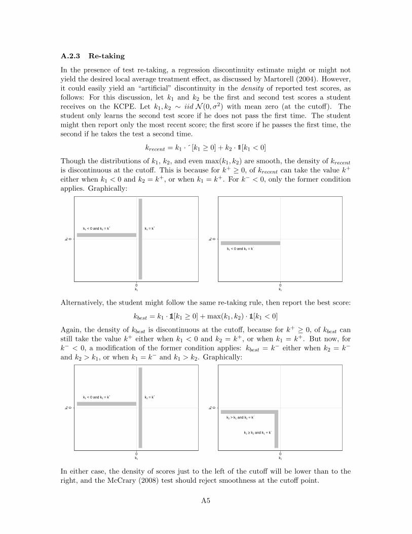
A.2.3 Re-taking

In the presence of test re-taking, a regression discontinuity estimate might or might notyield the desired local average treatment effect, as discussed by Martorell (2004). However,it could easily yield an “artificial” discontinuity in the density of reported test scores, asfollows: For this discussion, let k1 and k2 be the first and second test scores a studentreceives on the KCPE. Let k1, k2 ∼ iid N (0, σ2) with mean zero (at the cutoff). Thestudent only learns the second test score if he does not pass the first time. The studentmight then report only the most recent score; the first score if he passes the first time, thesecond if he takes the test a second time.

krecent = k1 · 1[k1 ≥ 0] + k2 · 1[k1 < 0]

Though the distributions of k1, k2, and even max(k1, k2) are smooth, the density of krecentis discontinuous at the cutoff. This is because for k+ ≥ 0, of krecent can take the value k+

either when k1 < 0 and k2 = k+, or when k1 = k+. For k− < 0, only the former conditionapplies. Graphically:

k1 < 0 and k2 = k+ k1 = k+

0k 2

0k1

k1 < 0 and k2 = k−

0k 2

0k1

Alternatively, the student might follow the same re-taking rule, then report the best score:

kbest = k1 · 1[k1 ≥ 0] + max(k1, k2) · 1[k1 < 0]

Again, the density of kbest is discontinuous at the cutoff, because for k+ ≥ 0, of kbest canstill take the value k+ either when k1 < 0 and k2 = k+, or when k1 = k+. But now, fork− < 0, a modification of the former condition applies: kbest = k− either when k2 = k−

and k2 > k1, or when k1 = k− and k1 > k2. Graphically:

k1 < 0 and k2 = k+ k1 = k+

0k 2

0k1

k2 > k1 and k2 = k−

k1 ≥ k2 and k1 = k−

0k 2

0k1

In either case, the density of scores just to the left of the cutoff will be lower than to theright, and the McCrary (2008) test should reject smoothness at the cutoff point.

A5

A.3 Proofs

Lemma 1. EU ss and EUfs are increasing in q, the probability of finding a job in eachperiod.

Proof. Let W = wself/farmi − cu and let Ewbesti = W + ∆W where ∆W > 0. Then:

EU =1

1− δ + qδ·(W +

qδ

1− δ(W + ∆W

))=W + q δ

1−δ(W + ∆W

)1− δ + qδ

d

dq

(W + q δ

1−δ(W + ∆W

)1− δ + qδ

)=

δ1−δ

(W + ∆W

)(1− δ + qδ)− δ

(W + q δ

1−δ(W + ∆W

))(1− δ + qδ)2

To establish the sign of this expression, we only need to establish the sign of the numerator:

δ

1− δ(W + ∆W

)(1− δ)− δW =δ

(W + ∆W

)− δW = δ∆W > 0

Thus, ddqEU > 0.

Implication 2. Pr[EUfs > EU ss] is weakly increasing in µ: If, for a particular agent, theeffective wage from farming is lower than that from self-employment, then the probabilitythat expected utility from searching for a job while farming exceeds that from searching fora job while self-employed is (weakly) increasing in the geometric mean of wage offers.

Proof. Begin by expanding the inequality, EUfs > EU ss:

1

1− δ + qfδ·(wfarmi − cu +

qfδ

1− δEwbesti

)>

1

1− δ + qsδ·(wselfi − cu +

qsδ

1− δEwbesti

)(1− δ + qsδ)

(wfarmi − cu +

qfδ

1− δEwbesti

)> (1− δ + qfδ)

(wselfi − cu +

qsδ

1− δEwbesti

)(1− δ)

(wfarmi − wselfi +

δ∆q

1− δEwbesti

)> δ

(qfwselfi − qswfarmi + ∆qcu

)Reorganizing these terms:

(1− δ) δ∆q

1− δEwbesti > δ

(qfwselfi − qswfarmi + ∆qcu

)+ (1− δ)

(wselfi − wfarmi

)δ∆qEwbesti > δ

((qs + ∆q)wselfi − qswfarmi + ∆qcu

)+ (1− δ)

(wselfi − wfarmi

)δ∆qEwbesti > δ

(∆qwselfi + ∆qcu

)+ (1− δ + qsδ)

(wselfi − wfarmi

)δ∆qEwbesti > δ∆q(wselfi + cu) + (1− δ + qsδ)

(wselfi − wfarmi

)δ∆q

(Ewbesti − wselfi − cu

)> (1− δ + qsδ)

(wselfi − wfarmi

)Thus, Pr[EUfs > EU ss] = Pr

[(wselfi − wfarmi

)< δ∆q

(Ewbesti − wselfi − cu

)]. By defi-

nition, Ewbesti is increasing (linearly) in Ewemp>wr

i , and Ewemp>wr

i is in turn increasing

in µ. Conditional on any values of {wselfi , wfarmi }, following from the laws of probability,Pr[EUfs > EU ss] is weakly increasing in µ.

A6

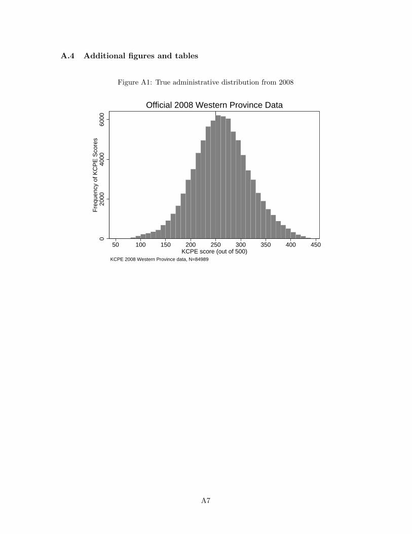
A.4 Additional figures and tables

Figure A1: True administrative distribution from 2008

020

0040

0060

00F

requ

ency

of K

CP

E S

core

s

50 100 150 200 250 300 350 400 450KCPE score (out of 500)

KCPE 2008 Western Province data, N=84989

Official 2008 Western Province Data

A7

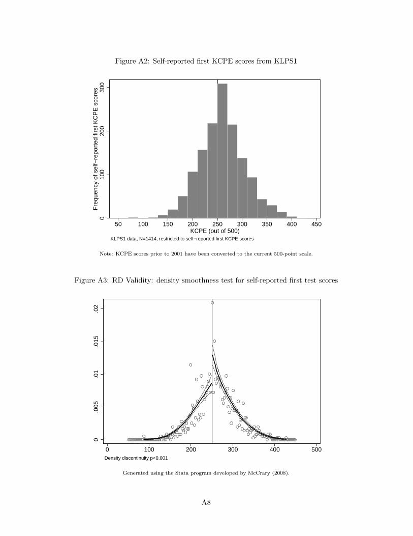
Figure A2: Self-reported first KCPE scores from KLPS1

010

020

030

0F

requ

ency

of s

elf−

repo

rted

firs

t KC

PE

sco

res

50 100 150 200 250 300 350 400 450KCPE (out of 500)

KLPS1 data, N=1414, restricted to self−reported first KCPE scores

Note: KCPE scores prior to 2001 have been converted to the current 500-point scale.

Figure A3: RD Validity: density smoothness test for self-reported first test scores

0.0

05.0

1.0

15.0

2

0 100 200 300 400 500Density discontinuity p<0.001

Generated using the Stata program developed by McCrary (2008).

A8

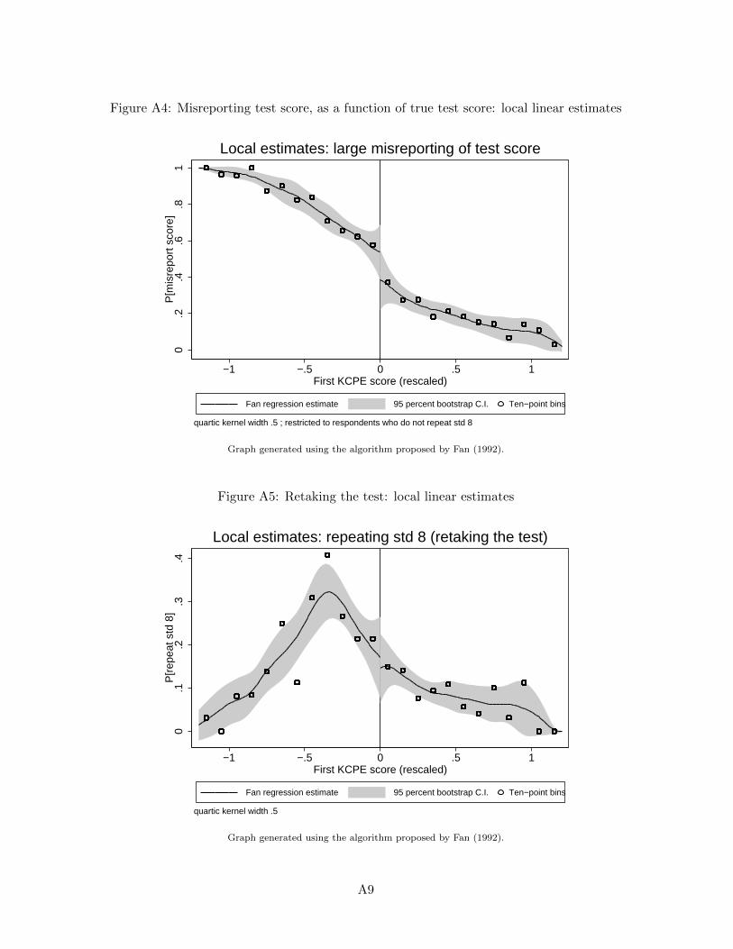
Figure A4: Misreporting test score, as a function of true test score: local linear estimates

0.2

.4.6

.81

P[m

isre

port

sco

re]

−1 −.5 0 .5 1First KCPE score (rescaled)

Fan regression estimate 95 percent bootstrap C.I. Ten−point bins

quartic kernel width .5 ; restricted to respondents who do not repeat std 8

Local estimates: large misreporting of test score

Graph generated using the algorithm proposed by Fan (1992).

Figure A5: Retaking the test: local linear estimates

0.1

.2.3

.4P

[rep

eat s

td 8

]

−1 −.5 0 .5 1First KCPE score (rescaled)

Fan regression estimate 95 percent bootstrap C.I. Ten−point bins

quartic kernel width .5

Local estimates: repeating std 8 (retaking the test)

Graph generated using the algorithm proposed by Fan (1992).

A9

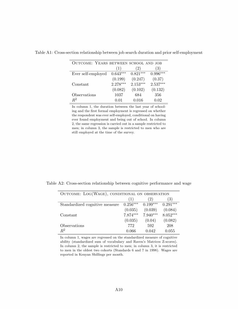
Table A1: Cross-section relationship between job search duration and prior self-employment

Outcome: Years between school and job(1) (2) (3)

Ever self-employed 0.643∗∗∗ 0.821∗∗∗ 0.996∗∗∗

(0.199) (0.247) (0.37)Constant 2.278∗∗∗ 2.153∗∗∗ 2.537∗∗∗

(0.082) (0.102) (0.132)Observations 1037 684 356R2 0.01 0.016 0.02

In column 1, the duration between the last year of school-ing and the first formal employment is regressed on whetherthe respondent was ever self-employed, conditional on havingever found employment and being out of school. In column2, the same regression is carried out in a sample restricted tomen; in column 3, the sample is restricted to men who arestill employed at the time of the survey.

Table A2: Cross-section relationship between cognitive performance and wage

Outcome: Log(Wage), conditional on observation(1) (2) (3)

Standardized cognitive measure 0.256∗∗∗ 0.199∗∗∗ 0.291∗∗∗

(0.035) (0.039) (0.084)Constant 7.874∗∗∗ 7.940∗∗∗ 8.052∗∗∗

(0.035) (0.04) (0.082)Observations 772 592 208R2 0.066 0.042 0.055

In column 1, wages are regressed on the standardized measure of cognitiveability (standardized sum of vocabulary and Raven’s Matrices Z-scores).In column 2, the sample is restricted to men; in column 3, it is restrictedto men in the oldest two cohorts (Standards 6 and 7 in 1998). Wages arereported in Kenyan Shillings per month.

A10

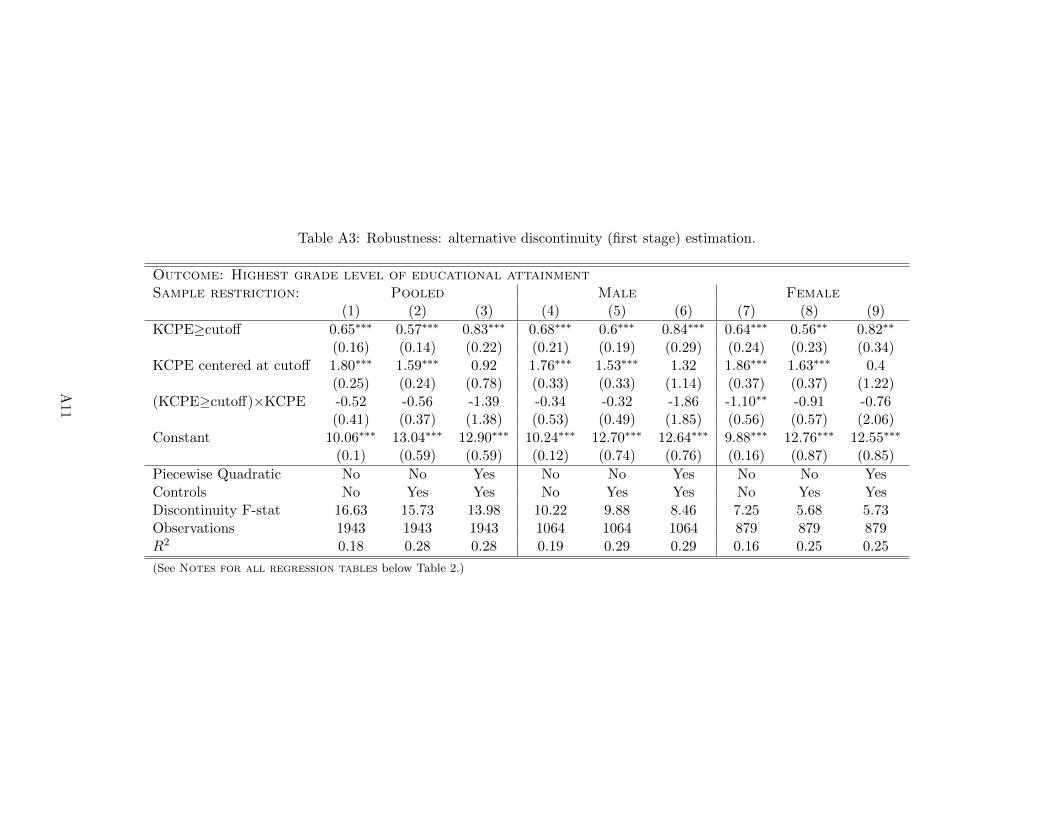
Table A3: Robustness: alternative discontinuity (first stage) estimation.

Outcome: Highest grade level of educational attainmentSample restriction: Pooled Male Female

(1) (2) (3) (4) (5) (6) (7) (8) (9)

KCPE≥cutoff 0.65∗∗∗ 0.57∗∗∗ 0.83∗∗∗ 0.68∗∗∗ 0.6∗∗∗ 0.84∗∗∗ 0.64∗∗∗ 0.56∗∗ 0.82∗∗

(0.16) (0.14) (0.22) (0.21) (0.19) (0.29) (0.24) (0.23) (0.34)KCPE centered at cutoff 1.80∗∗∗ 1.59∗∗∗ 0.92 1.76∗∗∗ 1.53∗∗∗ 1.32 1.86∗∗∗ 1.63∗∗∗ 0.4

(0.25) (0.24) (0.78) (0.33) (0.33) (1.14) (0.37) (0.37) (1.22)(KCPE≥cutoff)×KCPE -0.52 -0.56 -1.39 -0.34 -0.32 -1.86 -1.10∗∗ -0.91 -0.76

(0.41) (0.37) (1.38) (0.53) (0.49) (1.85) (0.56) (0.57) (2.06)Constant 10.06∗∗∗ 13.04∗∗∗ 12.90∗∗∗ 10.24∗∗∗ 12.70∗∗∗ 12.64∗∗∗ 9.88∗∗∗ 12.76∗∗∗ 12.55∗∗∗

(0.1) (0.59) (0.59) (0.12) (0.74) (0.76) (0.16) (0.87) (0.85)

Piecewise Quadratic No No Yes No No Yes No No YesControls No Yes Yes No Yes Yes No Yes YesDiscontinuity F-stat 16.63 15.73 13.98 10.22 9.88 8.46 7.25 5.68 5.73Observations 1943 1943 1943 1064 1064 1064 879 879 879R2 0.18 0.28 0.28 0.19 0.29 0.29 0.16 0.25 0.25

(See Notes for all regression tables below Table 2.)

A11

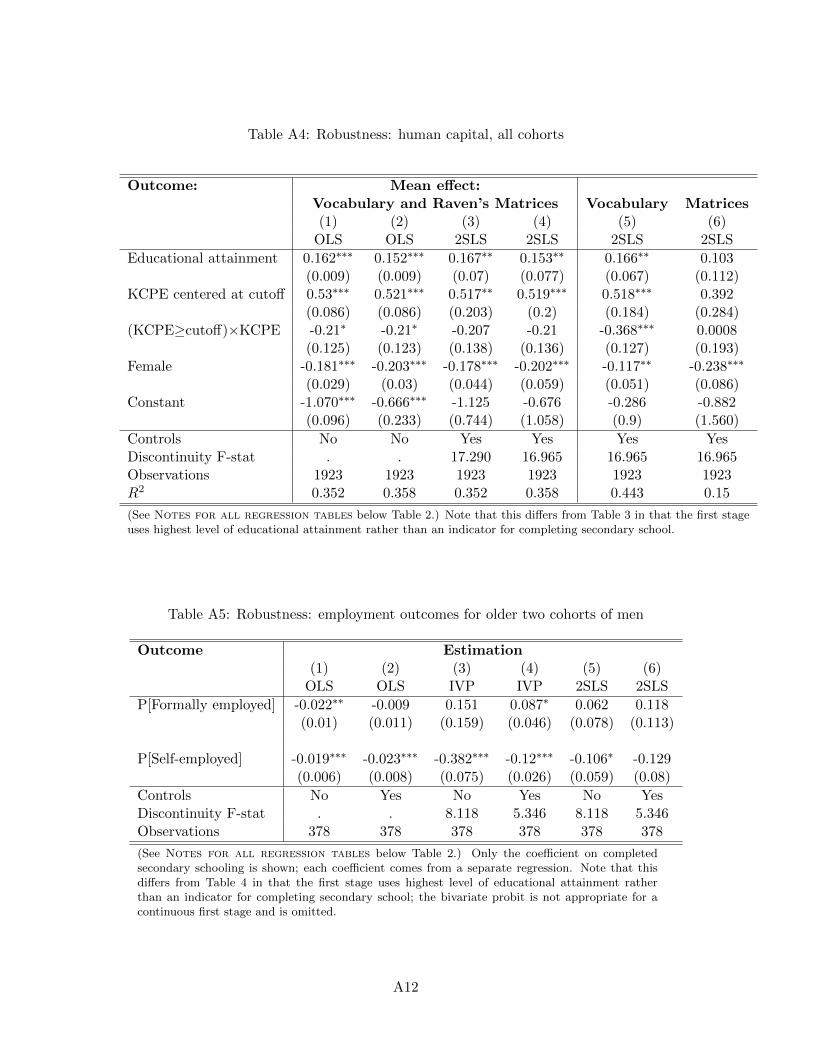
Table A4: Robustness: human capital, all cohorts

Outcome: Mean effect:Vocabulary and Raven’s Matrices Vocabulary Matrices(1) (2) (3) (4) (5) (6)

OLS OLS 2SLS 2SLS 2SLS 2SLS

Educational attainment 0.162∗∗∗ 0.152∗∗∗ 0.167∗∗ 0.153∗∗ 0.166∗∗ 0.103(0.009) (0.009) (0.07) (0.077) (0.067) (0.112)

KCPE centered at cutoff 0.53∗∗∗ 0.521∗∗∗ 0.517∗∗ 0.519∗∗∗ 0.518∗∗∗ 0.392(0.086) (0.086) (0.203) (0.2) (0.184) (0.284)

(KCPE≥cutoff)×KCPE -0.21∗ -0.21∗ -0.207 -0.21 -0.368∗∗∗ 0.0008(0.125) (0.123) (0.138) (0.136) (0.127) (0.193)

Female -0.181∗∗∗ -0.203∗∗∗ -0.178∗∗∗ -0.202∗∗∗ -0.117∗∗ -0.238∗∗∗

(0.029) (0.03) (0.044) (0.059) (0.051) (0.086)Constant -1.070∗∗∗ -0.666∗∗∗ -1.125 -0.676 -0.286 -0.882

(0.096) (0.233) (0.744) (1.058) (0.9) (1.560)

Controls No No Yes Yes Yes YesDiscontinuity F-stat . . 17.290 16.965 16.965 16.965Observations 1923 1923 1923 1923 1923 1923R2 0.352 0.358 0.352 0.358 0.443 0.15

(See Notes for all regression tables below Table 2.) Note that this differs from Table 3 in that the first stageuses highest level of educational attainment rather than an indicator for completing secondary school.

Table A5: Robustness: employment outcomes for older two cohorts of men

Outcome Estimation(1) (2) (3) (4) (5) (6)

OLS OLS IVP IVP 2SLS 2SLS

P[Formally employed] -0.022∗∗ -0.009 0.151 0.087∗ 0.062 0.118(0.01) (0.011) (0.159) (0.046) (0.078) (0.113)

P[Self-employed] -0.019∗∗∗ -0.023∗∗∗ -0.382∗∗∗ -0.12∗∗∗ -0.106∗ -0.129(0.006) (0.008) (0.075) (0.026) (0.059) (0.08)

Controls No Yes No Yes No YesDiscontinuity F-stat . . 8.118 5.346 8.118 5.346Observations 378 378 378 378 378 378

(See Notes for all regression tables below Table 2.) Only the coefficient on completedsecondary schooling is shown; each coefficient comes from a separate regression. Note that thisdiffers from Table 4 in that the first stage uses highest level of educational attainment ratherthan an indicator for completing secondary school; the bivariate probit is not appropriate for acontinuous first stage and is omitted.

A12

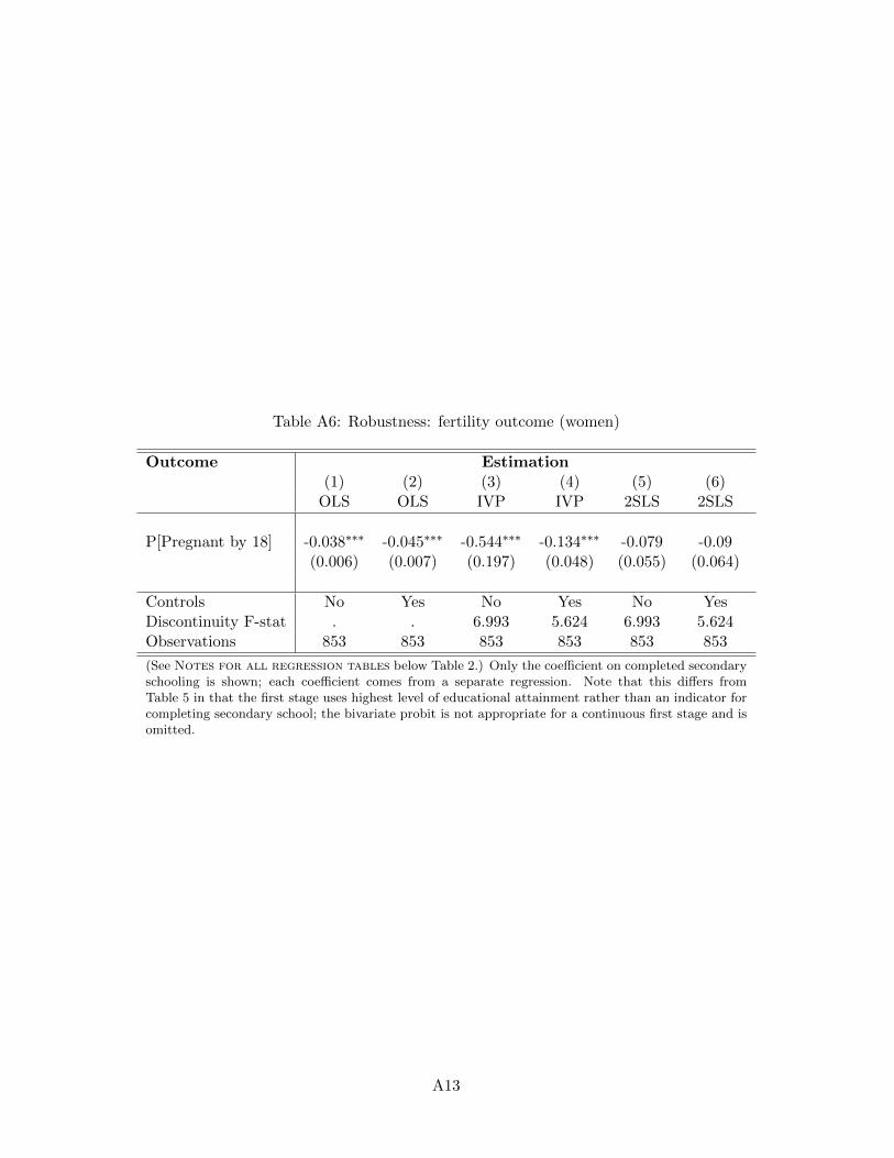
Table A6: Robustness: fertility outcome (women)

Outcome Estimation(1) (2) (3) (4) (5) (6)

OLS OLS IVP IVP 2SLS 2SLS

P[Pregnant by 18] -0.038∗∗∗ -0.045∗∗∗ -0.544∗∗∗ -0.134∗∗∗ -0.079 -0.09(0.006) (0.007) (0.197) (0.048) (0.055) (0.064)

Controls No Yes No Yes No YesDiscontinuity F-stat . . 6.993 5.624 6.993 5.624Observations 853 853 853 853 853 853

(See Notes for all regression tables below Table 2.) Only the coefficient on completed secondaryschooling is shown; each coefficient comes from a separate regression. Note that this differs fromTable 5 in that the first stage uses highest level of educational attainment rather than an indicator forcompleting secondary school; the bivariate probit is not appropriate for a continuous first stage and isomitted.

A13

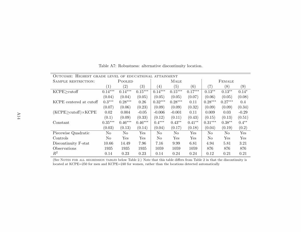
Table A7: Robustness: alternative discontinuity location.

Outcome: Highest grade level of educational attainmentSample restriction: Pooled Male Female

(1) (2) (3) (4) (5) (6) (7) (8) (9)

KCPE≥cutoff 0.14∗∗∗ 0.14∗∗∗ 0.15∗∗∗ 0.14∗∗∗ 0.15∗∗∗ 0.17∗∗∗ 0.13∗∗ 0.13∗∗ 0.14∗

(0.04) (0.04) (0.05) (0.05) (0.05) (0.07) (0.06) (0.05) (0.08)KCPE centered at cutoff 0.3∗∗∗ 0.28∗∗∗ 0.26 0.32∗∗∗ 0.28∗∗∗ 0.11 0.28∗∗∗ 0.27∗∗∗ 0.4

(0.07) (0.06) (0.23) (0.09) (0.09) (0.32) (0.09) (0.09) (0.34)(KCPE≥cutoff)×KCPE 0.02 0.004 -0.05 -0.006 -0.001 0.11 0.009 0.03 -0.29

(0.1) (0.09) (0.33) (0.12) (0.11) (0.43) (0.15) (0.13) (0.51)Constant 0.35∗∗∗ 0.46∗∗∗ 0.46∗∗∗ 0.4∗∗∗ 0.43∗∗ 0.41∗∗ 0.31∗∗∗ 0.38∗∗ 0.4∗∗

(0.03) (0.13) (0.14) (0.04) (0.17) (0.18) (0.04) (0.19) (0.2)

Piecewise Quadratic No No Yes No No Yes No No YesControls No Yes Yes No Yes Yes No Yes YesDiscontinuity F-stat 10.66 14.49 7.96 7.16 9.99 6.81 4.94 5.81 3.21Observations 1935 1935 1935 1059 1059 1059 876 876 876R2 0.14 0.23 0.23 0.14 0.24 0.24 0.12 0.21 0.21

(See Notes for all regression tables below Table 2.) Note that this table differs from Table 2 in that the discontinuity islocated at KCPE=250 for men and KCPE=240 for women, rather than the locations detected automatically

A14

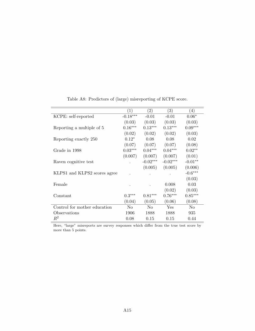
Table A8: Predictors of (large) misreporting of KCPE score.

(1) (2) (3) (4)

KCPE: self-reported -0.18∗∗∗ -0.01 -0.01 0.06∗

(0.03) (0.03) (0.03) (0.03)Reporting a multiple of 5 0.16∗∗∗ 0.13∗∗∗ 0.13∗∗∗ 0.09∗∗∗

(0.02) (0.02) (0.02) (0.03)Reporting exactly 250 0.12∗ 0.08 0.08 0.02

(0.07) (0.07) (0.07) (0.08)Grade in 1998 0.03∗∗∗ 0.04∗∗∗ 0.04∗∗∗ 0.02∗∗

(0.007) (0.007) (0.007) (0.01)Raven cognitive test . -0.02∗∗∗ -0.02∗∗∗ -0.01∗∗

(0.005) (0.005) (0.006)KLPS1 and KLPS2 scores agree . . . -0.6∗∗∗

(0.03)Female . . 0.008 0.03

(0.02) (0.03)Constant 0.3∗∗∗ 0.81∗∗∗ 0.76∗∗∗ 0.85∗∗∗

(0.04) (0.05) (0.06) (0.08)

Control for mother education No No Yes NoObservations 1906 1888 1888 935R2 0.08 0.15 0.15 0.44

Here, “large” misreports are survey responses which differ from the true test score bymore than 5 points.

A15