Embed Size (px)
Citation preview
IMPACT OF THE BUILT ENVIRONMENT ON MICROCLIMATE IN SAN JOSÉ,
CALIFORNIA
A Thesis submitted to the faculty of
San Francisco State University
In partial fulfillment of
the requirements for
the Degree
Master of Arts
In
Geography: Resource Management and Environmental Planning
by
Reese Noel Hann
San Francisco, California
December 2020

Copyright by
Reese Noel Hann
2020
CERTIFICATION OF APPROVAL
I certify that I have read Impact of the Built Environment on Microclimate in San José,
California by Reese Noel Hann, and that in my opinion this work meets the criteria for approving
a thesis submitted in partial fulfillment of the requirement for the degree Master of Arts in
Geography: Concentration in Resource Management and Environmental Planning at San
Francisco State University.
Andrew Oliphant, Ph.D.
Professor,
Thesis Committee Chair / Date
Sara Baguskas, Ph.D.
Assistant Professor / Date
Impact of the Built Environment on Microclimate in San José, California
Reese Noel Hann
San Francisco, California
2020
Most cities have heterogeneous land uses, which produce internal variability in the Urban Heat
Island (UHI). Urban heating coupled with rising global temperatures leads to an increase in heat-
related illnesses, decrease in human comfort and increase in energy consumption. This study
investigates the spatial variability of the UHI at the neighborhood scale in San José, California
using a mobile transect to measure temperature differences. Sampling sites were classified into
Local Climate Zones (LCZ) based on vegetation, impervious fractions, and building morphology.
Average evening temperature differences were 1.5 °C warmer downtown than an urban park and
0.5 °C cooler in a well vegetated neighborhood compared to neighborhood with similar built urban
form, but different amounts of vegetation. Stronger wind speeds decreased temperatures
differences between LCZs. Results are consistent with theory that vegetation provides cooling via
evapotranspiration and that increases in the built urban form lead to increases in temperature. LCZs
with increased impervious and building surface fractions experienced increased temperatures
whereas LCZs with increased pervious fractions experienced cooler temperatures.

v
PREFACE AND/OR ACKNOWLEDGEMENTS
This research was created out of my love for San José, observations made from my own front yard,
and the communities affected by the differences in temperature. I will always be looking out for
socioeconomic and environmental justice for the most vulnerable peoples.
Thank you to all the special people and family who supported me and made my research possible.
➢ To Andrew Oliphant, who has taught me so much and has been ever patient. He took on
my research proposal, born out of our love for climatology and my tenacious interest in
urban planning and the intersection of the science which informs our decisions.
➢ To Michael Breidert who used his amazing GIS skills to make this research using the
LCZ system possible. He created maps and provided us with the geospatial analysis of
characteristics in the built urban form of San José.
➢ And to my spouse, Adrian De La Cerda, who drove me around in a manual transmission
car on city streets, in stop and go traffic, for 24 transects at all times of the day. Adrian
has been constant support throughout my education and is the reason I am here today.

vi
TABLE OF CONTENTS
LIST OF TABLES .................................................................................................................................................... vii
LIST OF FIGURES ................................................................................................................................................. viii
LIST OF APPENDICES ............................................................................................................................................xi
Introduction ................................................................................................................................................................. 1
Methods ...................................................................................................................................................................... 15
2.1 Study Area ........................................................................................................................................................ 15
2.2 Instrument Design ............................................................................................................................................. 17
2.3 Mobile Transect ................................................................................................................................................ 19
2.4 Local Climate Zone Classification .................................................................................................................... 20
2.5 Temperature Corrections & Data Analysis ....................................................................................................... 23
Results ......................................................................................................................................................................... 26
3.1 Classifying Local Climate Zones in San José ................................................................................................... 26
3.2 General Meteorological Conditions during the Field Study ............................................................................. 31
3.3 Temperature Differences Observed between the LCZs .................................................................................... 32
3.4 Comparing Differences in Ambient Evening and Afternoon Temperature across LCZs ................................. 37
3.5 Comparing Wind Speed in the Evenings .......................................................................................................... 39
3.6 Impact of Ambient Temperatures on Temperature Departures ......................................................................... 42
3.7 Diurnal Variations in Temperature Departure .................................................................................................. 45
Discussion ................................................................................................................................................................... 47
4.1 Local Climate Zone Classifications .................................................................................................................. 49
4.2 Park and Lake Cool Island Effects .................................................................................................................... 51
4.3 The Built Urban Form and UHI ........................................................................................................................ 54
Conclusions ................................................................................................................................................................ 58
References .................................................................................................................................................................. 62
Appendices ................................................................................................................................................................. 67

vii
LIST OF TABLES
Table Page
1. Table 1: Collection of studies with multiple LCZs similar to San José with temperatures
taken after sunset. Temperature differences, UHI magnitudes, UHI intensity, and
temperature averages based on reporting method of selected study ………….….…….….11
2. Table 2: Measurements and definitions of properties required to classify LCZs. Rows 1-7
represent geometric and surface cover properties. Rows 8-10 represent thermal, radiative,
and metabolic processes (Stewart et al., 2012) .....................................................................21
3. Table 3: Visual physical characteristics of LCZ classifications from Stewart & Oke and site
selections in San José, California (2012). Aerial satellite imagery provided by Michael
Breidert (2020). Classification graphics retrieved from Stewart & Oke (2012). Eye level
photos taken from Google Earth street view ……………..............…………………….….27
4. Table 4: LCZ names, classifications, physical properties, site measurements, and the LCZ
indicators for each classification according to Stewart & Oke (2012). Pervious, impervious,
and building percentages obtained by Michael Breidert. Aspect ratio and average element
height obtained by Michael Breidert, Andrew Oliphant, and Reese Hann ..........................28

viii
LIST OF FIGURES
Figures Page
1. Figure 1: LCZ classification types. LCZ 1-10 represent built urban forms while LCZ A-F
represent natural land cover properties. Figure taken from Betchel et al., page 4 (2017) .….7
2. Figure 2: Local Climate Zone subclassification process. Figure taken from page 14, Stewart
& Oke (2012).……………….…………………………………………….……………….9
3. Figure 3: Map of the San Francisco Bay conurbation in California with San José located in
the South ………………………………………………………………….……………….16
4. Figure 4: Topographic imagery of the relief in the San Francisco Bay Area with San José
situated in the south valley. Imagery provided by Michael Breidert. …………...…………17
5. Figure 5: Vehicle with Mounted PCV pipe containing the type E thermocouple, HMP60
thermistor hygristor, Apogee infrared radiometer, and 12-volt fan ……………………….18
6. Figure 6: Map of LCZ locations in San José. Transect route occurred East to West beginning
at the lake and ending downtown. Map provided by Michael Breidert......…………….….20
7. Figure 7: Raw temperature data, corrected data, and linear time correction for a transect
collected on July 27th, 2019 from 21:10 to 22:09 with the LCZ measurement sites indicated
by the green boxes ………………………………………………………………………...24
8. Figure 8: General wind direction (azimuth degrees), wind speed (m s-1), and temperature (°
C), conditions during the 24 transects. Transects 1-17 occurred in the evening, 18-22
surveyed in the afternoon, and transects 23 and 24 occurring in the early morning ……….32
9. Figure 9: Mean evening temperature departure for each LCZ location. The transect mean
was obtained for 13 evening transects surveyed with a wind direction from the North or
Northwest ………………………………………………………………………………....33
10. Figure 10: Mean afternoon temperature departure for each LCZ location. The site mean was
obtained from five afternoon transects surveyed with a wind direction from the North or
Northwest …………………………………………………………………………………35
11. Figure 11: Mean evening temperature departure for four LCZ locations using all 17 evening
ix
transects from all wind directions ………………………………………………………....36
12. Figure 12: Box plots for each sampled LCZ showing the distribution of temperature
variability for 13 evening transects with the wind direction from the North to Northwest.
The LCZ average transect median (red line) is inside of the box. The top of the blue box
represents the 75th percentile and the bottom represents the 25th percentile. The black lines
extending from the boxes represent the tails of the temperature distribution and the red marks
represent outliers.................................................................................... ………………….38
13. Figure 13: Box plots for each sampled LCZ showing the distribution of temperature
variability for all five afternoon transects with the wind direction from the North to
Northwest. The LCZ average transect median (red line) is inside of the box. The top of the
blue box represents the 75th percentile and the bottom represents the 25th percentile. The
black lines extending from the boxes represent the tails of the temperature distribution and
the red marks represent outliers ...........................................................................................39
14. Figure 14: Mean temperature departure for 13 evening transects on 6 windier evenings and
7 less windy evenings. The site temperature mean was obtained for the 13 evening transects
surveyed with North to Northwest wind direction. The average wind speed was 3.29 m s-1.
The average wind speed for windier evenings was 4.1 m s-1 and for less windy evenings, 2.6
m s-1. ……………….............................................................................…………...……...40
15. Figure 15: Mean temperature departure for four LCZ locations for 17 evening transects on
6 windier evenings and 11 less windy evenings. The site temperature mean was obtained for
all 17 evening transects surveyed. The average wind speed was 2.99 m s-1. The average wind
speed for windy evenings was 4.1 m s-1 and for less windy evenings, 2.4 m s-1.……...........42
16. Figure 16: Mean temperature departure for each LCZ location on evenings with average
temperature above or below 25 °C. The site mean was obtained from temperature transects
with a wind direction from the North or Northwest . The mean transect temperature for the
transect above 25 °C was 32.2 °C and on evenings below 25 °C the mean was 20.8 °C ......43
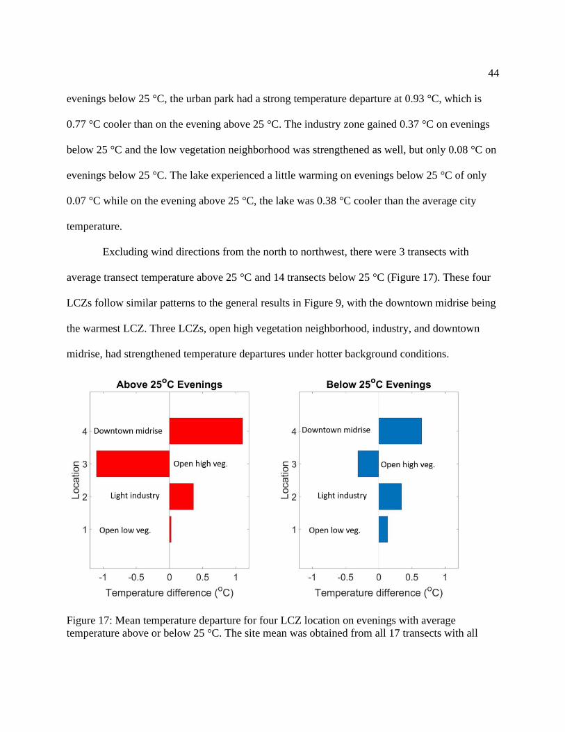
17. Figure 17: Mean temperature departure for four LCZ location on evenings with average
temperature above or below 25 °C. The site mean was obtained from all 17 transects with
all wind directions. The mean transect temperature for evenings above 25 °C was 30.7 °C
and on evenings below 25 °C the mean was 20.3 °C. …………..................……………….44

x
18. Figure 18: Diurnal temperature distribution for four LCZ on July 21, 2019 ……………...46
19. Figure 19: Diurnal temperature distribution for each LCZ on July 27, 2019 …………….46

xi
LIST OF APPENDICES
Appendix Page
1. Appendix A: Evening pairwise comparisons of temperature differences between LCZs with
P Values indicating significant or not significant differences between LCZs ......................67
2. Appendix B: Afternoon pairwise comparisons of temperature differences between LCZs
with P Values indicating significant or not significant differences between LCZs ..............68

1
Introduction
Urban areas are becoming more densely populated globally (United Nations (UN), 2018).
Of the world’s population, 54% live in urban areas and this number is expected to increase to
66% by 2050 (UN, 2018). As urban populations increase, there is usually an increase in the built
urban form, i.e., buildings, parking lots, etc., which change the landscape and impact city
temperatures (Kleerekoper et al., 2011). Urban planning, which address increases in density,
urban form, and population should integrate climate into their conversation as these
modifications alter the climate regimes in cities (Gago et al., 2013). Each city needs individual
analysis to identify each microscale climate differences, which is unique and affected by specific
characteristics in the built urban form. Urban development plans, whether for future development
or renovations of space, should factor in microclimate in order to optimize public use of space
(Kleerekoper et al., 2011).
The Urban Heat Island (UHI) effect is the result of changes in the surface energy budget
due to replacement of the natural environment by the built environment (Oke, 1987). Intra-urban
UHI studies seek to explain temperature differences based on the built urban form and sample
different urban environments. These samples address different levels of heating based on urban
design factors such as building height, amount of vegetation, or spacing between buildings.
Planning and mitigation efforts should be informed by an understanding of which urban design
factors affect the UHI and Human Thermal Comfort (HTC). HTC is a measurement at the scale
of the human body, which is used to understand felt temperature and the experience of a person
in a particular place (Oke, 1987).

2
HTC will be affected by climate change in addition to urban form. Climate change
models based on two different emission scenarios project an increase in temperatures from 2.4
°C to 4.3 °C by 2100 (Dahl et al., 2019). Under both emissions scenarios, the annual number of
days with heat indices exceeding 37.8 °C (100 °F) and 40.6 °C (105 °F) are projected to double
and triple, respectively, compared to a 1971–2000 baseline (Dahl et al., 2019). In July of 1995,
there were a total of 514 heat related deaths with an additional 254 deaths likely caused by heat
in Chicago, Illinois (Whitman et al., 1997). This increase in heating coupled with the UHI leads
to an increase in intensity and frequency of heat waves which are linked to extreme heat related
illnesses and increased mortality rates (Bowler et al., 2010).
The UHI is defined as the air temperature differences between urban and surrounding
rural landscapes: UHI=Tu-Tr, where Tu is urban air temperature and Tr is rural air temperature
(Oke, 1987). In most regions, the comparative rural landscape is comprised of permeable
surfaces, increased surface water storage, and vegetation similar to the city site in its pre-urban
natural state (Oke, 2006). Vegetation promotes evapotranspiration, a key process in cooling the
surrounding area, as plants absorb solar radiation and transform this energy into latent heat rather
than sensible heat via transpiration (Bowler et al., 2010). Shade from trees cools the
microclimate by intercepting solar radiation, which reduces warming on the ground surface or of
the surrounding air (Bowler et al., 2010). Therefore, areas with more vegetation and soil, such as
urban parks, can produce cool air pools within a broader UHI driven by higher
evapotranspiration rates (Bowler et al., 2010). The Park Cool Island (PCI) is defined as PCI=Tu-
Tp, where Tu is urban air temperature and Tp is park air temperature (Spronken-Smith & Oke,
1998).
3
The built urban form is constructed with a variety of materials, most of which have
different thermal and radiative properties than the previously existing landscape (Morgan et al.,
1977). These urban materials store much greater amounts of heat during the day and release that
heat at night causing urban areas to be warmer than surrounding rural regions, particularly in the
hours after sunset (Terjung & Louie, 1973). However, not all urban areas worldwide have the
same UHI due to the vast differences in materials, form, weather conditions, climate, vegetation,
and building density. Other than differences in the urban form and materials, the amount of
vegetation, soil and surface water in a city directly impacts the amount of moisture in the air
(Terjung et al., 1970). Additionally, anthropogenic activities, such as running air conditioning or
driving cars, add heat to the city scape (Iamarino et al., 2012).
The built urban form of a city alters the Surface Energy Balance (SEB), defined as:
Q*+QF=QH+QE+ΔQS, (Eq. 1)
where Q* is net allwave radiation, QF is the anthropogenic heat flux, QH is the sensible
heat flux, QE is the latent heat flux, and ΔQs, the change in heat storage (Oke, 1987). In a city,
QH and ΔQS, are typically larger and QE smaller than in surrounding rural energy budgets
(Morgan et al., 1977; Oke, 1987). The reduction in vegetation and soil water storage decreases
QE, which reduces cooling of a region via evapotranspiration (Gunawardena et al., 2017). The
additional energy this provides during the middle of the day enhances both QH and ΔQS, which
warms the urban surface layer atmosphere. This increase in QH and ΔQS in cities directly
increases warming causing the UHI.
Cities also experience an increase ΔQS due to more heat penetrating the urban materials
during the day when Q* is high (Oke, 1987). The increase in ΔQS is caused by greater absorption

4
of solar radiation due to radiation trapping and reflection by building walls and vertical surfaces.
This reduces daytime convective losses in the canopy layer which are instead delayed and
released at night (Stewart & Oke, 2012). The thermal properties of typical building materials
absorb incoming radiation whereas vegetation has lower temperatures due to evapotranspiration
and the conversion of incoming radiation instead of absorption (Shashua-Bar & Hoffman, 2000).
The anthropogenic heat flux, QF, is derived from three main human activities: in
buildings from heating or air conditioning systems, transportation, and from human metabolism
(Iamarino et al., 2012). In the greater London area in England, the average annual anthropogenic
heat flux was 10.9 W m-2 in 2005-2009, a minimal amount compared to incoming daily solar
radiation which ranges by latitude in the hundreds of W m-2 (Iamarino et al., 2012).
As the SEB changes across urban form, so does the temperature. The SEB changes
between neighborhoods that vary in the amount of vegetation. Areas with higher vegetation
cover have a higher ratio of QE to QH which can lead to a cooling of the surrounding
environment (Oke, 1987). Areas with increased QH are produce higher temperatures and a higher
UHI (Oke, 1987). Cities are complex and comprised of all these variations in the built urban
form.
The terms ‘urban’ and ‘rural’ are too limiting when studying UHI in cities as each
individual area of a city has unique physical properties which contribute to a microclimate that is
distinct from other areas or neighborhoods of the same city (Stewart & Oke, 2012). Previous
UHI studies, which typically surveyed simple temperature differences between urban and rural
areas, missed the complexity of the built urban form in a city and the factors which either add or
mitigate heat (Oke 2006). To better understand the microclimate differences within a city, the

5
UHI became more commonly evaluated in terms of temperature differences between different
types of urban form or density, such as in Nagano, Japan (Sakakibara, & Matsui, 2005), Tel
Aviv, Israel (Shashua-Bar & Hoffman, 2000), and Singapore (Wong & Yu, 2005). These studies
addressed temperature differences based on vegetation, population and built density, and city
zoning. In Japan, researchers were interested in the connection between densely inhabited
districts (DID) and the effect of this built urban form on the UHI. It was found in six settlements,
city size indices and DID are highly correlated to temperature differences between urban and
rural landscapes.
In Israel, a summer survey was conducted to collect temperature data from 11 urban
green areas with trees to analyze the cooling effect of trees and found an average of 2.8 K cooler
in urban green areas with trees with a range from 1 K to 4 K (Shashua-Bar & Hoffman, 2000). In
2005 in Singapore, researchers identified urban form differences such as the airport, forest,
residential, and industry and conducted a mobile transect to identify temperature differences
across the city (Wong & Yu, 2005). A connection was found between lower temperatures and
vegetation while densely built urban forms such as the CBD (Central Business District) had the
highest temperatures (Wong & Yu, 2005).
Additionally, in some cities it is difficult to find a rural representative area. The rural-
urban boundary continues to expand with development and population growth. The boundary
can also be contained by valleys and/or water bodies, such as the study site of this research, San
José, California. This is problematic when obtaining UHI values as the goal is to avoid
extraneous microclimate influences, and the thermal properties of water and increases in
elevation such as orographic effects are met with changes in temperature due to physical

6
geography rather than differences in the built urban form compared to the previous natural
environment (Oke, 2006).
Due to the complex form of cities, the Local Climate Zone (LCZ) Classification
framework was proposed in 2012, which identifies differences in the built urban form and land
cover types within cities to measure the intra-urban variability of the UHI (Stewart & Oke,
2012). This framework permits LCZ comparisons relative to the overall city temperature, which
helps identify UHI magnitude differences within each distinct zone. The LCZ classifications are
based on geometric and surface cover properties including, but not limited to: sky view factor
(SVF), aspect ratio, building surface fraction, impervious and pervious surface fraction, height of
roughness elements, and terrain roughness class using Davenport et al.’s (2000) classification for
city and country landscapes (Stewart & Oke, 2012).
LCZs are split into ten built types, which are commonly found in the urban form
worldwide (Figure 1)(Betchel et al., 2017). These range in density, stories, size, natural or
constructed materials, and use (Stewart & Oke, 2012). There are seven LCZ based on land cover
types, which are natural landscapes (Stewart & Oke, 2012). These include dense trees, scattered
trees, brush or scrub, low plants, bare rock or paved, bare soil or sand, and water (Figure
1)(Betchel et al, 2017). There are also four ephemeral land cover properties to account for
seasonal differences: snow cover, bare trees, dry ground, and wet ground (Stewart & Oke, 2012).

7
Figure 1: LCZ classification types. LCZ 1-10 represent built urban forms while LCZ A-F
represent natural land cover properties. Figure taken from Betchel et al.,(2017, p.4).
Classifying LCZs consists of collecting metadata and defining the thermal source area.
Metadata can be collected via site visits, but more often now, metadata is collected from datasets
obtained from and collected by local agency or municipalities, governmental organizations,
nonprofits, or from ESRI, the Environmental Science Research Institute. These datasets are

8
analyzed using geographic information systems (GIS) which consists of land cover/land use
maps, aerial photographs, and satellite imagery (Stewart & Oke, 2012).
Defining the thermal source area of each LCZ is imperative as the source area is the
region monitored or observed by the temperature sensor, often called the footprint or circle of
influence (Oke, 2006; Stewart & Oke, 2012). The source area determines if the designated region
is representative of the LCZ classification. Consideration of the thermal source area includes
wind direction as a key factor. The source area should extend upwind from the instrumentation
for accurate temperature measurements of a designated LCZ (Oke, 2006). There are 10
measurements suggested by Stewart and Oke (2012) to determine LCZ classification. However,
studies use varying amounts of the measurements with most using between five to eight, (e.g.,
Stevan et al., 2013; Alexander & Mills, 2014; Thomas et al., 2014; Leconte et al., 2015; Lehnert
et al., 2015; Wang et al., 2016; Skarbit et al., 2017; Yang et al., 2017; Kotharkar & Bagade,
2018; Aminipouri et al., 2019).
The LCZ regime was meant to classify structures, such as buildings, trees, or housing,
worldwide based on their climatic properties (Betchel et al., 2015). The classification system is
meant to be inherently generic yet contain select well-engineered features so that it may cover
cities across climates and ecoregions worldwide (Demuzere et al., 2019). Local differences in
cities such as the layout of city streets, cultural differences in the density and spacing of
buildings, historic design styles, vegetation, types, and buildings materials are not considered in
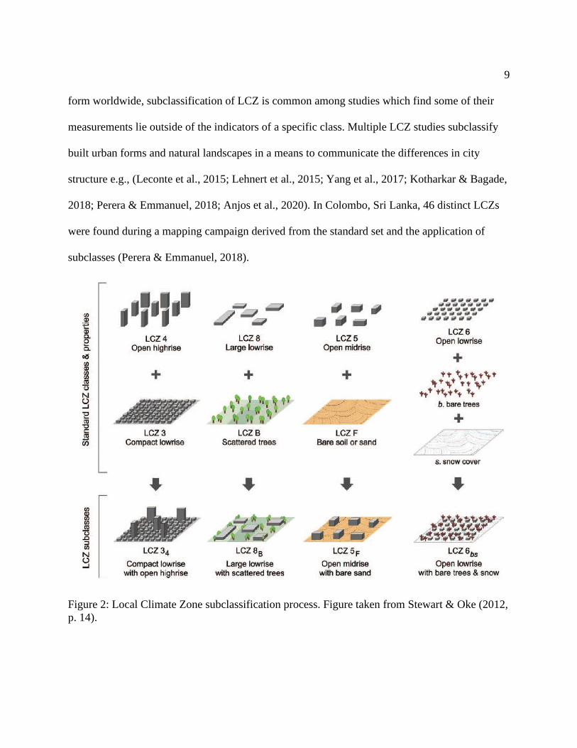
the framework (Betchel et al., 2015). The framework encourages users to create subclass sites
which deviate from the standard set and represent a combination of built or land cover types
(Figure 2) (Stewart & Oke, 2012; Demuzere et al., 2019). Due to variances in the built urban
9
form worldwide, subclassification of LCZ is common among studies which find some of their
measurements lie outside of the indicators of a specific class. Multiple LCZ studies subclassify
built urban forms and natural landscapes in a means to communicate the differences in city
structure e.g., (Leconte et al., 2015; Lehnert et al., 2015; Yang et al., 2017; Kotharkar & Bagade,
2018; Perera & Emmanuel, 2018; Anjos et al., 2020). In Colombo, Sri Lanka, 46 distinct LCZs
were found during a mapping campaign derived from the standard set and the application of
subclasses (Perera & Emmanuel, 2018).
Figure 2: Local Climate Zone subclassification process. Figure taken from Stewart & Oke (2012,
p. 14).

10
Currently, there are multiple ways in which studies report LCZ findings. Often reported
values are UHI magnitudes or intensity. Studies which report these values choose a LCZ, usually
the coolest in temperature, and report the UHI from the chosen LCZ as a reference. Differences
from the LCZs collective average temperatures are most common and most desirable to use
when completing inter-city comparisons. When inter-city comparison is lacking, the single city
analysis of average temperature differences between LCZs is applied as ΔTairLCZ x-y. In ΔTairLCZ
x-y reporting, there is no city average. Reporting of differences between LCZs is difficult to use in
inter-city comparisons as it only works if the city in question has the same LCZs as the city in
the study. Some studies also report average temperature of each LCZs and compare each LCZ
average against another LCZ temperature average in their study. This reporting can be used,
although it does not provide a temperature difference from an average and therefore can be
difficult to apply in inter-city comparisons.
Table 1: Collection of studies with multiple LCZs similar to San José with temperatures taken
after sunset. Temperature difference, UHI magnitude, UHI intensity, and temperature averages
based on reporting method of selected study.
LCZ 1 LCZ 2 LCZ 8 LCZ 6 LCZ A/B LCZ D LCZ G Reference
3.1 K 3 K 1.8 K 1.2 K -0.2 K 2 K
(Yang et al., 2017)
Nanjing, China
UHI Magnitude
3.13 °C 1.92 °C
(Thomas et al., 2014
Kochi, India
UHI Intensity
0.3 °C 24.8°C* 24.8 °C*
(Chieppa et al., 2018)
Auburn, AL, USA
UHI Intensity
1.4 °C 24.9 °C* 26 °C*
(Chieppa et al., 2018)
Opelika, AL, USA
UHI Intensity
2.5 K 0.8 K (-0.4) K (-0.6) K
(-1) K (-2.6) K (Stewart & Oke, 2012)

11
LCZ 1 LCZ 2 LCZ 8 LCZ 6 LCZ A/B LCZ D LCZ G Reference
Vancouver, BC,
Canada
Temperature
Difference
2.1 °C 0.97 °C (-2.17) °C
(Alexander & Mills,
2014) Dublin, Ireland
Temperature
Difference
0.7 °C 0.6 °C 0.4 °C (-0.3) °C (-0.8) °C
(Anjos et al., 2020)
Londrina, Brazil
Temperature
Difference
1.1 °C 0.3 °C (-7) °C (-3.5) °C 0.4 °C
(Wang et al., 2018)
Las Vegas, NV, USA
Temperature
Difference
1.2 °C (-0.1) °C (-0.5) °C (-2) °C (-0.8) °C
(Wang et al., 2018)
Phoenix, AZ, USA
Temperature
Difference
*Chieppa et al. (2018) did not report water or forest temperatures as a UHI intensity, only
average temperatures which were not statistically significant from the LCZ 6.
Table 2 is a selection of LCZ studies which had two or more LCZs that are also found in
San José, California. Generally, LCZs 1, 2, and 8 have higher temperatures, temperature
differences, or UHI magnitudes than LCZ 6, open low rise development. In cities where LCZ 1,
2, and 8 were surveyed, LCZ 1 and 2 have higher temperatures, temperature differences, or UHI
magnitudes than LCZ 8. Lowest temperatures, temperatures differences, or UHI magnitudes are
found in natural landscapes A, B, D, or G (Table 2). These findings are consistent with the
framework’s assessment of LCZs in Vancouver, BC, which shows that positive temperature
departures occur in built urban forms and natural environments have negative temperature
departures (Table 2)(Stewart & Oke, 2012).

12
These results indicate that higher temperatures are found in areas with increased built
urban density including increases in building surface area and building surface fraction. The
alteration of the surface energy balance in LCZs 1,2, and 8 causes a lack of evapotranspiration
and an increase in energy absorption into building materials. These LCZ study results also show
that areas with vegetation or water, produce cooler temperatures due to evapotranspiration and
pervious land cover, which is found in the form of natural environments. These findings are
consistent with theory of the UHI and PCI effect; changes from the natural environment to the
built environment cause warmer temperatures. Similarly, in LCZ 6s surveyed in Table 2, only
two reported temperatures below average, but still not equal to temperature differences in LCZs
A-G.
An advanced search on Google Scholar (https://scholar.google.com/) procures
publication data from 2012, the initial publishing of the LCZ framework, to 2020, showing that
there are over 1,250 results which mention LCZs and the Urban Heat Island using a Boolean
search function. These articles range from reviews, case studies, models, classification best
practices and more. According to Xue et al. (2020), there have been over 800 citations of the
original framework and publication of over 220 articles in 2019 alone. Xue et al. (2020)
attributes this growth due to the diffusion of urban climatology into applied fields such as urban
and regional planning, building and construction technology, engineering, and ecology
concluding that LCZ classification addresses more than urban temperature; rather it is a gateway
to sustainable urban development and human health.
Due to the wide range of applicability and interest in the LCZ scheme, mobile
measurement case studies are not well represented in the LCZ literature. Out of 610 articles
13
published and analyzed about the LCZ classification scheme, only 109 focused on the surface
urban heat island, land surface temperature, MODIS (Moderate Resolution Imaging
Spectroradiometer), and the urban heat island effect (Xue et al., 2020). Within these 109 articles,
methods such as MODIS can be used to evaluate temperature using imagery rather than field
measurements. The four most popular publication categories in LCZ literature other than the
UHI effect included: 1. OTC (outdoor thermal comfort) and PET (physiologically equivalent
temperature), 2. remote sensing and convolutional neural networks, 2. SUEWS (Surface Urban
Energy and Water Balance Scheme) and WRF (Weather Research and Forecasting Model), and
4. Crowdsourcing air temperature, cyber-infrastructure, and citizen weather station (Xue et al.,
2020).
In an analysis of 50 cities using the LCZ investigating surface UHI, there was no city
studied with a Csb Köppen climate classification. (Bechtel et al., 2019). Additionally, all these
cities from the 50 city comparison used MODIS instead of field measurements to assess the UHI.
The dominate Köppen climate classifications surveyed in the 50 city comparison were Cfa, Cfb,
Dfa, Dwa, Dfb, and Aw, most of which are represented in Table 2, which compares LCZ results
from studies using field methods (Betchel et al., 2019). Additionally, Las Vegas, NV and
Phoenix, AZ have a classification of Bwh and are represented since Arizona State University is
the leading institution publishing LCZ related literature with over 112 publications as of July
2020 (Xue et al., 2020).
With relatively limited examples of field measurements and a lack of representation of
Mediterranean climates, San José, California provides a good example of a Csb Köppen climate
classification, which is a warm summer Mediterranean climate. This case study adds to the

14
collection of LCZ literature addressing a particular climate regime and adds a sample of built
urban forms and their temperature deviations from San José.
The broader objective of this study was to investigate the spatial variability of ambient air
temperature at 2 m at the neighborhood-scale in San José, California, USA during summer.
Specific objectives were to obtain detailed temperature differences between neighborhoods using
a mobile measurement system, and to characterize the local climate zone of each using the
Stewart and Oke (2012) LCZ classification system. Additionally, temperature samples were
taken in the afternoon and morning to identify changes over the diurnal cycle. Analysis was
conducted asking how temperature responds to heat events and how temperature changes due to
differences in wind speed.
This study explores variability in the built urban form and amount of vegetation to reveal
temperature differences and patterns of the LCZs caused by land use in urban environments
within the same city. This information will be compared with similar LCZ studies conducted in
other cities with different climates, but similar built environments. We aim to place the San José
findings in the context of intra-urban temperature measurements made in comparative
neighborhoods worldwide which use the LCZ classification system to draw broader conclusions
about urban heating and the implications for planning further urban growth.
We hypothesize that expected results would include higher temperatures in the minimally
vegetated neighborhood compared to the highly vegetated neighborhood regardless of similar
urban form. Additionally, the highest overall temperature in the city is expected to be produced
by densely built urban form, the downtown region. Temperature differences will be greatest
15
following sunset, weakened during windier conditions, and strengthened under hotter
background weather conditions.
Methods
2.1 Study Area
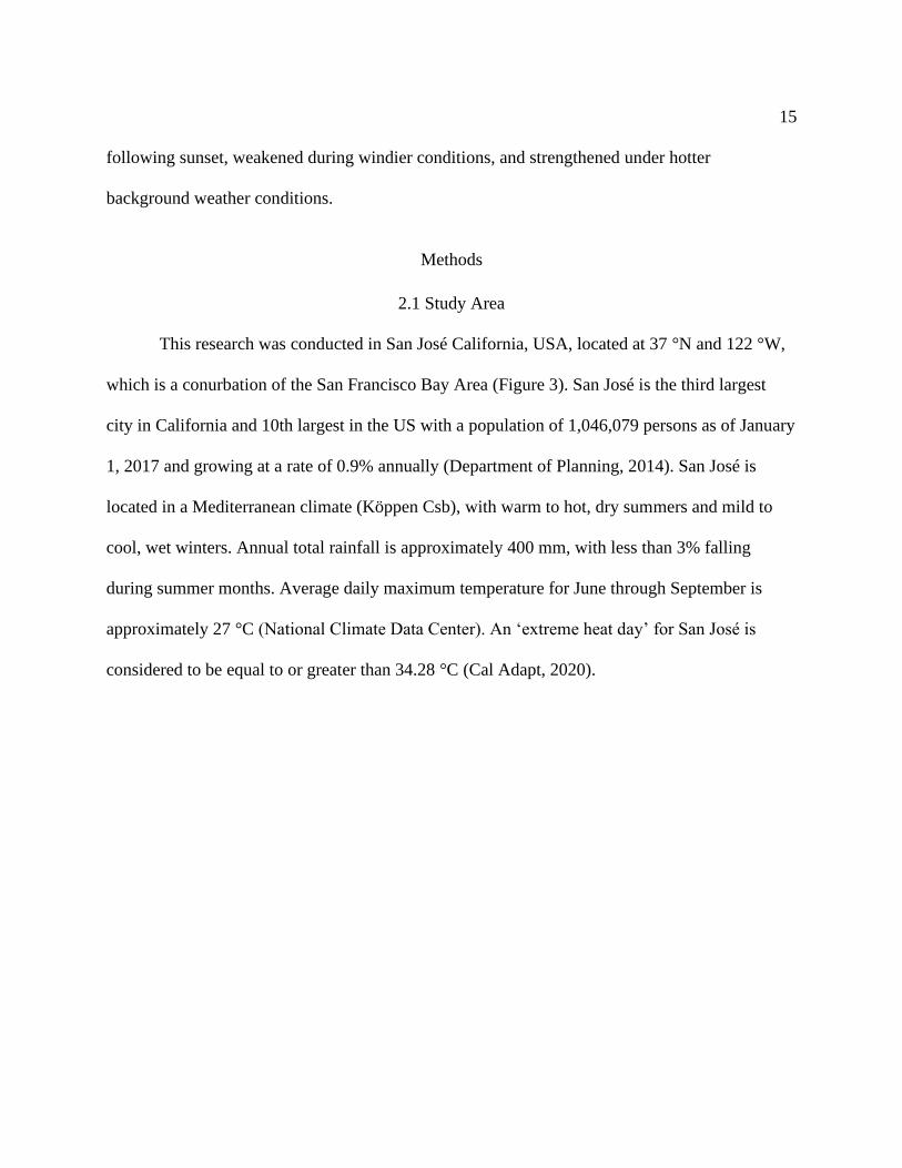
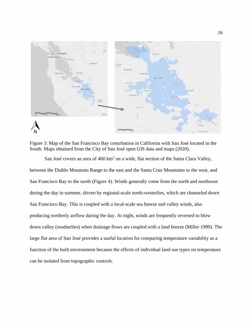
This research was conducted in San José California, USA, located at 37 °N and 122 °W,
which is a conurbation of the San Francisco Bay Area (Figure 3). San José is the third largest
city in California and 10th largest in the US with a population of 1,046,079 persons as of January
1, 2017 and growing at a rate of 0.9% annually (Department of Planning, 2014). San José is
located in a Mediterranean climate (Köppen Csb), with warm to hot, dry summers and mild to
cool, wet winters. Annual total rainfall is approximately 400 mm, with less than 3% falling
during summer months. Average daily maximum temperature for June through September is
approximately 27 °C (National Climate Data Center). An ‘extreme heat day’ for San José is
considered to be equal to or greater than 34.28 °C (Cal Adapt, 2020).
16
Figure 3: Map of the San Francisco Bay conurbation in California with San José located in the
South. Maps obtained from the City of San José open GIS data and maps (2020).
San José covers an area of 460 km2 on a wide, flat section of the Santa Clara Valley,
between the Diablo Mountain Range to the east and the Santa Cruz Mountains to the west, and
San Francisco Bay to the north (Figure 4). Winds generally come from the north and northwest
during the day in summer, driven by regional-scale north-westerlies, which are channeled down
San Francisco Bay. This is coupled with a local-scale sea breeze and valley winds, also
producing northerly airflow during the day. At night, winds are frequently reversed to blow
down valley (southerlies) when drainage flows are coupled with a land breeze (Miller 1999). The
large flat area of San José provides a useful location for comparing temperature variability as a
function of the built environment because the effects of individual land use types on temperature
can be isolated from topographic controls.

17
Figure 4: Topographic imagery of the relief in the San Francisco Bay Area with San José situated
in the south valley. Imagery provided by Michael Breidert.
2.2 Instrument Design
Measurements were made during mobile traverses across the city using an instrumented
passenger vehicle. The vehicle was fitted with T-shaped PCV pipe, attached to the roof rack
(Figure 5). The structure raised the measurement height to 2 m, 32 cm above the vehicle roof and
the horizontal pipe channeled airflow directly to the sensors. In the center of the PCV pipe,
exposed to the channeled airflow was a type-E thermocouple and a Vaisala HMP60 thermistor
and hygristor (Vaisala Inc, Helsinki, Finland). Vehicle mounted sensors were at 1.8 m above
ground level, aspirated both naturally by vehicle motion and using a 12V fan, positioned at the
rear of the PVC tubing so as to continuously draw air from the front of the tubes past the sensors.
Attached to the outside of the PVC pipe pointing laterally to the right of the car, an Apogee
thermal infrared radiometer (Apogee Instruments Inc., Logan Utah) was mounted. The

18
radiometer was directed towards surfaces to the right of the vehicle capturing the built urban
environment, such as houses, parkland, or buildings, which the vehicle passed by.
The instruments were wired into a CR1000 Campbell Scientific data logger (Campbell
Scientific Inc. Logan, Utah), which was programmed using Loggernet software. The datalogger
recorded air temperature from the type E thermocouple and HMP60 thermistor, relative humidity
from the HMP60 hygristor, and surface temperature from the infrared radiometer. The datalogger
was programmed with a sampling frequency of one second, and each study area was sampled for
three minutes for a total of 180 samples.
Figure 5: Vehicle with Mounted PCV pipe containing the type E thermocouple, HMP60
thermistor hygristor, Apogee infrared radiometer, and 12-volt fan.
The same instruments were used in each transect and each study site. Assuming
instrument error is small and systematic, it is unlikely to play a role in the inter-site differences
observed in this study. However, in order to check instrument performance prior to data
collection, the instruments were compared with three other similar sensors on a campus rooftop

19
for one week, storing 10-minute averages derived from one-second samples. The instruments
responded to temperature and humidity differences equivalently over the period, with mean
absolute differences <0.3 °C for the thermistor, <0.15 °C for the thermocouple and <2.5% for
relative humidity observed by the hygristor. In all cases the coefficient of determination between
the instruments used in this study and their comparison sensors was greater than 0.98.
2.3 Mobile Transect
Mobile measurements were collected along 24 transects between June 2019 and August
2019 during the following time periods: 17 in the evening following sunset (2100-2300 PDT),
five during the early afternoon (~1400 PDT) day, and two in the early morning (~0400-0500).
Each of the six LCZs was sampled by driving continuously within the designated area at a speed
of approximately 50 km h-1 for three minutes (Figure 6). For the park and lake sites, due to
access constraints at evening, observations were made while the vehicle was parked at the
downwind border of the parklands (assuming the prevailing NW flow). Each transect took
approximately 45 to 70 minutes to conduct.

20
Figure 6: Map of LCZ locations in San José. Transect route occurred East to West beginning at
the lake and ending downtown. Map provided by Michael Breidert.
2.4 Local Climate Zone Classification
LCZ classification for San José used Google Earth and ArcGIS to determine the
characteristics of the urban form. Each LCZ underwent analysis of five geometric and surface
cover properties: aspect ratio, building fraction, impervious fraction, pervious fraction, and
average element height (Table 2).

21
Table 2: Measurements and definitions of properties required to classify LCZs. Rows 1-7
represent geometric and surface cover properties. Rows 8-10 represent thermal, radiative, and
metabolic processes (Stewart et al., 2012).
Measurement Definition from Stewart & Oke (2012)
1 Sky View Factor Ratio of the amount of sky hemisphere visible from ground
level to that of an unobstructed hemisphere
2 Aspect Ratio Mean height to width ratio of street canyons in LCZ 1-7,
building spacing in LCZ 8-10, and/or tree spacing in LCZ A-G
3 Building surface fraction Ratio of building plan area to total plan area
4 Impervious Surface Fraction Ratio of impervious plan area to total plan area
5 Pervious Surface Fraction Ratio of pervious plan area to total plan area
6 Height of roughness element Geometric average of building heights and/or trees
7 Terrain Roughness class Davenport classification of effective terrain roughness
8 Surface Admittance Ability of surface to accept or release heat
9 Surface Albedo Amount of solar radiation reflected by a surface
10 Anthropogenic Heat Output Mean annual heat flux density
The spacing of urban elements for the aspect ratio was obtained using the ruler function
in Google Earth in all LCZs. In each LCZ, more than 30 random sample observations were
obtained for spacing between either buildings, trees, or street canyons. Additionally, element
height for trees was obtained from Google Earth using the same methodology. To obtain the
aspect ratio in the urban park and lake, tree element height average was divided by tree spacing
average to obtain the aspect ratio.
The element height for buildings, however, was obtained from an open source building
footprint GIS dataset from the City of San José. The average building height was found in each
LCZ and was obtained by dividing the number of unique buildings by the total of all building
heights in each LCZ. To obtain the aspect ratio in the downtown, both neighborhoods, and the

22
industrial LCZs, the building element height average was divided by either street canyon width
average or building spacing average.
The building surface fraction was obtained from the same data set as building heights by
finding the total surface area of buildings in each LCZ. This total building area was then divided
by the total area of each LCZ. This number was multiplied by 100 to obtain the building surface
fraction as a percentage.
The impervious and pervious surface fractions data sets were obtained from the National
Land Cover Database (NLCD) maintained by the Multi-Resolution Land Characteristics
Consortium which includes partners such as the United States Geological Survey (USGS), the
National Oceanic and Atmospheric Administration (NOAA) , the Environmental Protection
Agency (EPA), and more. 30m resolution cells were designated with an impervious or pervious
count. These cells were extracted for each LCZ and counted as a total sum. The cells were
categorized as either pervious or impervious and divided by the sum and multiplied by 100 to
find the percentage of pervious and impervious surface for each LCZ. Building surface fraction
was subtracted from the impervious surface fraction to create the impervious ground surface
fraction. The impervious ground, pervious ground, and building surface fraction equate to 100
percent of the total area of each LCZ.
In this study, five out of ten LCZ indicators were explored: aspect ratio, building surface
fraction, impervious surface fraction, pervious surface fraction, and height of roughness
elements. This study did not estimate five LCZ indictors which included: sky view factor, terrain
roughness class, surface admittance, surface albedo, and anthropogenic heat output.

23
A higher parent class should represent the standard set and one or more classes can be
assigned a subclass based on LCZ measurements (Stewart & Oke, 2012). This higher parent
classification was assigned to each LCZ based on visual physical characteristics of the urban
form and site measurements which were dominant in the LCZ region. Subclassifications, which
represent secondary and tertiary characteristics of the built or natural urban forms, were found
within our LCZs. These subclassifications were assigned based on the measurements which were
outside of the indictors for the parent class assigned to each LCZ. LCZ subclassifications are
ordered numerically by differences in the built urban form, 1-10, and then alphabetically by
differences in the natural environment, A-G.
2.5 Temperature Corrections & Data Analysis
Due to the temporal changes in temperature over the duration of each transect,
temperature corrections were required for accurate comparison between LCZs. In a similar study
that used a mobile vehicle system to quantify air temperature variation in an urban area, Leconte
et al. (2015) accounted for the natural variation in air temperature by applying a linear time
correction using the initial air temperature at the start of their sampling session as a reference
temperature. Similarly, we used a linear regression model to account for the natural temperature
change based on each transects starting temperature. Figure 7 shows the one-second temperature
samples from a single transect captured after sunset. A linear decrease in temperature can be
observed, associated with the early nocturnal cooling part of the diurnal cycle (blue line, Figure
7). A linear regression model (orange line) was fit to the variation in temperature in order to find
the linear rate of change over the transect. This rate of cooling was used to correct all samples

24
observed after the initial sample (purple line), which was used to assess the relative temperature
differences between LCZs.
Figure 7: Raw temperature data, corrected data, and linear time correction for a transect collected
on July 27th, 2019 from 21:10 to 22:09 with the LCZ measurement sites indicated by the green
boxes.
Meteorological data was also downloaded from the MesoWest network of automated
weather stations for a station located at the San José Airport, which provided fixed 5-minute
average meteorological data over the entire study period. These data were used to derive
background meteorological conditions during each transect, so that inter-LCZ climate
differences could be evaluated with respect to wind speed and direction, background temperature
and humidity.

25
MATLAB, an analysis software which uses matrix and array programming, was used to
process the data obtained from a total of 24 transects. For the two fixed measurement sites, the
urban park and the lake, the instruments were stationary and located to the South Southeast.
Therefore, observations only represented the intended LCZ for wind directions between 285° and
30° due to the location of the measurement site relative to the LCZ. There were 13 evening
transects with North to Northwest wind directions and all five afternoon transects also had North
to Northwest winds. All six LCZs were analyzed when the wind direction was between 285° and
30°.
Analysis of all 17 evening transects regardless of wind direction was also conducted but
excluded the lake and the urban park. These four LCZs, which did not need wind direction as a
consideration for accurate representation of their built urban forms, were the open high
vegetation neighborhood, open low vegetation neighborhood, downtown midrise, and the light
industry zone. Additionally, we examined the diurnal patterns of the six LCZs on two days in
late July 2019.
We compared air temperature between the different LCZs and the average temperature of
the city which was calculated as average air temperature per transect to estimate city-wide
temperature during each measurement session. The variability in the magnitude of UHI per LCZ
was calculated as the difference in air temperature between a given LCZ and the average mean of
all the LCZs sampled. This LCZ average replaces a rural reference site and shows the difference
between city temperature and neighborhood scale temperature (LCZs).
Investigation of the data collected also consisted of examining each location’s variability
to determine the range of temperatures within each location. To test for statistical differences in
26
evening temperature between sites, we performed an Analysis of Variance (ANOVA) and post-
hoc Tukey test using statistical software (RStudio, version 4.0.2).
Results
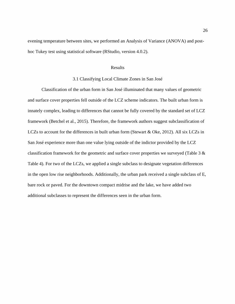
3.1 Classifying Local Climate Zones in San José
Classification of the urban form in San José illuminated that many values of geometric
and surface cover properties fell outside of the LCZ scheme indicators. The built urban form is
innately complex, leading to differences that cannot be fully covered by the standard set of LCZ
framework (Betchel et al., 2015). Therefore, the framework authors suggest subclassification of
LCZs to account for the differences in built urban form (Stewart & Oke, 2012). All six LCZs in
San José experience more than one value lying outside of the indictor provided by the LCZ
classification framework for the geometric and surface cover properties we surveyed (Table 3 &
Table 4). For two of the LCZs, we applied a single subclass to designate vegetation differences
in the open low rise neighborhoods. Additionally, the urban park received a single subclass of E,
bare rock or paved. For the downtown compact midrise and the lake, we have added two
additional subclasses to represent the differences seen in the urban form.
27
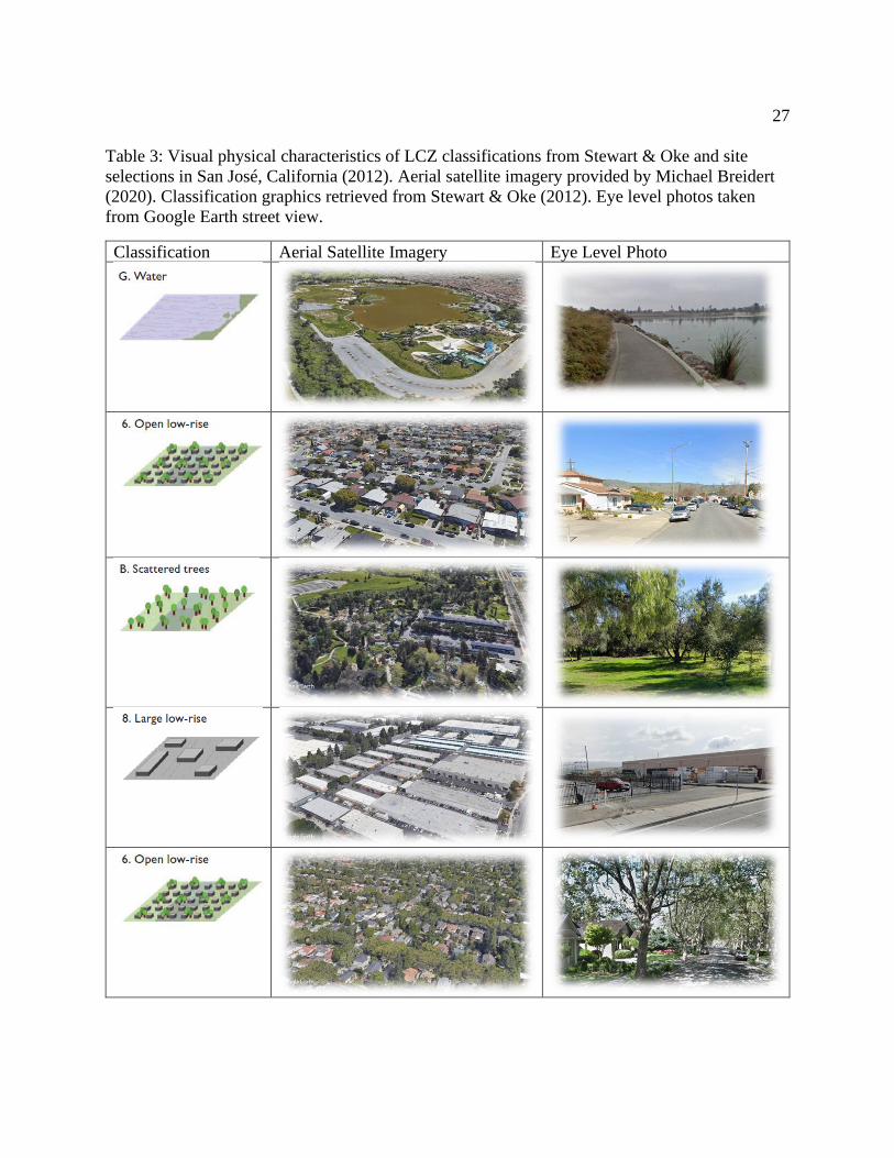
Table 3: Visual physical characteristics of LCZ classifications from Stewart & Oke and site
selections in San José, California (2012). Aerial satellite imagery provided by Michael Breidert
(2020). Classification graphics retrieved from Stewart & Oke (2012). Eye level photos taken
from Google Earth street view.
Classification Aerial Satellite Imagery Eye Level Photo

28
Classification Aerial Satellite Imagery Eye Level Photo
Table 4: LCZ names, classifications, physical properties, site measurements, and the LCZ
indicators for each classification according to Stewart & Oke (2012). Pervious, impervious, and
building percentages obtained by Michael Breidert. Aspect ratio and average element height
obtained by Michael Breidert, Andrew Oliphant, and Reese Hann.
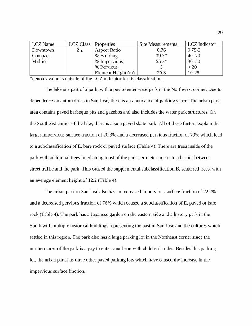
LCZ Name LCZ Class Properties Site Measurements LCZ Indicator
Lake GBE Aspect Ratio
% Building
% Impervious
% Pervious
Element Height (m)
0.08
0.7
20.3*
79*
12.2*
<0.1
<10
<10
>90
-
Open Low
Vegetation
Neighborhood
6E Aspect Ratio
% Building
% Impervious
% Pervious
Element Height (m)
0.14*
26.1
69.4*
4.5*
3.7
0.3-0.75
20-40
20–50
30-60
3–10
Urban Park BE Aspect Ratio
% Building
% Impervious
% Pervious
Element Height (m)
0.73
1.8
22.2
76
16.2*
0.25–0.75
<10
<10
>90
3–15
Light Industry 8 Aspect Ratio
% Building
% Impervious
% Pervious
Element Height (m)
0.17
31.3
67.7*
1
4.8
0.1–0.3
30–50
40–50
<20
3–10
Open High
Vegetation
Neighborhood
6B Aspect Ratio
% Building
% Impervious
% Pervious
Element Height (m)
0.25*
27.3
5.7*
67*
4.5
0.3-0.75
20-40
20–50
30-60
3–10
29
LCZ Name LCZ Class Properties Site Measurements LCZ Indicator
Downtown
Compact
Midrise
21E Aspect Ratio
% Building
% Impervious
% Pervious
Element Height (m)
0.76
39.7*
55.3*
5
20.3
0.75-2
40–70
30–50
< 20
10-25
*denotes value is outside of the LCZ indicator for its classification
The lake is a part of a park, with a pay to enter waterpark in the Northwest corner. Due to
dependence on automobiles in San José, there is an abundance of parking space. The urban park
area contains paved barbeque pits and gazebos and also includes the water park structures. On
the Southeast corner of the lake, there is also a paved skate park. All of these factors explain the
larger impervious surface fraction of 20.3% and a decreased pervious fraction of 79% which lead
to a subclassification of E, bare rock or paved surface (Table 4). There are trees inside of the
park with additional trees lined along most of the park perimeter to create a barrier between
street traffic and the park. This caused the supplemental subclassification B, scattered trees, with
an average element height of 12.2 (Table 4).
The urban park in San José also has an increased impervious surface fraction of 22.2%
and a decreased pervious fraction of 76% which caused a subclassification of E, paved or bare
rock (Table 4). The park has a Japanese garden on the eastern side and a history park in the
South with multiple historical buildings representing the past of San José and the cultures which
settled in this region. The park also has a large parking lot in the Northeast corner since the
northern area of the park is a pay to enter small zoo with children’s rides. Besides this parking
lot, the urban park has three other paved parking lots which have caused the increase in the
impervious surface fraction.
30
The open low vegetation neighborhood has a high impervious fraction of 69.4% and a
small pervious fraction of 4.5% with the minimum range for the pervious fraction in this type of
LCZ normally being 30% (Table 4). The subclass of E, paved or bare rock, was added to this
neighborhood. There is an abundance of paved front yards in this LCZ and backyards also may
be paved or covered in stone. Automobiles line the streets both day and night, with barely any
space left to park. Driveways also have multiple parked cars, vans, or trucks. Where there is
vegetation, it represents local plants, or occasional street trees.
The open high vegetation neighborhood has different urban form from the previously
mentioned neighborhood. There is an abundance of vegetation including pervious front yards,
smaller streets, and tree-lined avenues which called for a subclassification of B, scattered trees.
In San José, this neighborhood has a high pervious fraction of 67% and a small impervious
fraction of 5.7% with the minimum range for the impervious fraction in this type of LCZ
normally being 20% (Table 4). Street parking is not as common in this area and many homes
only use garage parking or may park a car or two on their driveway.
The industrial zone has a higher impervious percentage, 67.7%, than the indicator (Table
4). This region has many paved parking lots and streets in addition to large industrial buildings.
Finding any pervious surface is a challenge with trees placed along only major arterial streets.
This LCZ did not receive a subclassification even with a higher impervious percentage. The
building percentage was within the indicator as well as the pervious, albeit the value was
extremely low.
Downtown San José also has a higher percentage of impervious surfaces than the
indicator totaling at 55.3% which caused a subclassification of E, bare rock or paved surface

31
(Table 3). The surveyed LCZ 2 in San José has no urban parks. However, downtown San José
does have two urban parks, but these parks are located one block to the North and one block to
the South of the LCZ. There are also a few open surface parking lots within this LCZ boundary,
likely adding to the pervious fraction. While the building fraction is outside of the indictor, it
only falls short by 0.3%, likely due to the increased surface parking instead of built garages or
buildings (Table 3, Table 4). Downtown San José also received a subclassification of LCZ 1 for
compact high rise. In this LCZ, midrise buildings are dominant, but there is a healthy mix of
buildings over 10 stories (Table 3).
3.2 General Meteorological Conditions during the Field Study
Conditions during the 24 transects were typical of late summer conditions, dry and warm
with occasional hot days, and winds typically from the north to northwest during the day and
evening and from the south in the early morning (Figure 8). Wind speeds ranged from 1.2 m s-1
to 6.3 m s-1, and average temperatures ranged from 14.7 °C to 33.6 °C during the study period.
(Figure 8). Winds were consistently from the west to north except during two early morning
transects when weak down-valley flow existed with wind direction from the south to southeast
for Transects 23 and 24 (Figure 8). Most temperatures were typical of the summer in the mid 20
°Cs, but on a number of occasions, the temperatures reached greater than 30 °C even during the
evening transects. The early morning transects were significantly cooler.

32
Figure 8: General wind direction (azimuth degrees), wind speed (m s-1), and temperature (° C),
conditions during the 24 transects. Transects 1-17 occurred in the evening, 18-22 surveyed in the
afternoon, and transects 23 and 24 occurring in the early morning.
Wind direction in San José is typically from the North to Northwest, greater than 285°
and less than 30°, during the day and early evening. Wind direction during this study for
afternoon and evening transects was quite consistent and ranged from 246° to 339°.
3.3 Temperature Differences Observed between the LCZs
The deviation of each LCZ from the mean temperature of San José’s site mean is shown
in Figure 9. Here the temperature deviation refers to the differences between the 3-minute mean
corrected temperature of each study site and the average of all six study sites. Transects with
wind direction outside of San José’s typical North to Northwest flows were only included in
average temperature calculations for comparison between four LCZs, downtown midrise, open

33
high vegetation neighborhood, open low vegetation neighborhood, and the light industry, which
did not need these winds for a representative sample of their land use and urban form.
Figure 9: Mean evening temperature departure for each LCZ location. The transect mean was
obtained for 13 evening transects surveyed with a wind direction from the North or Northwest.
Generally, there are positive values in four of the six LCZs while the urban park and open
high vegetation neighborhood LCZs both experience lower than average temperatures (Figure 9).
The maximum difference in ambient air temperature occurred between the urban park and the
downtown midrise at 1.5 °C, with the downtown midrise experiencing the warmest temperatures
in San José at 0.6 °C above the transect average (Figure 9). The light industry zone was the
second warmest location with a temperature deviation of 0.4 °C and 1.3 °C higher than the urban
park. The open low vegetation neighborhood was 0.5 °C warmer than the open high vegetation
neighborhood. The two neighborhoods were classified in the same LCZ (Table 3), but the
warmer site has 62.5% less vegetation by area. The lake in the evening was near the average of

34
all sites and was 0.94 °C warmer than the urban park and most similar to the open low vegetation
neighborhood.
The coolest temperatures were found in the two most vegetated zones. The urban park
was the coolest zone at 0.9 °C below the average of the city, while the open high vegetation
neighborhood was approximately 0.3 °C cooler than the city average. The temperature difference
in the open high vegetation LCZ caused temperatures to be on average 0.5 °C cooler in this
neighborhood than the open low vegetation LCZ.
Afternoon temperature departure patterns in four of the six LCZ were opposite of their
evening values such as the hottest evening LCZ, downtown midrise, producing cool afternoon
temperatures, 0.6 °C below the city average (Figure 10). Similarly, the urban park was not the
coolest LCZ like in the evening, rather it was the hottest with a positive value of 1.3 °C above
the city average (Figure 10). The lake produced the coolest temperatures in the afternoon with an
average temperature difference from the mean of 1.4 °C contrary to its evening value which was
slightly above the city average (Figure 10). The temperature difference between the urban park
in the afternoon and the lake was 2.7 °C.

35
Figure 10: Mean afternoon temperature departure for each LCZ location. The site mean was
obtained from five afternoon transects surveyed with a wind direction from the North or
Northwest.
The open high vegetation neighborhood was similar to the open low vegetation
neighborhood in the afternoons, unlike in the evenings, producing a positive temperature
departure of 0.2 °C (Figure 10). The open low vegetation neighborhood was barely cooler than
the high vegetation neighborhood, slightly warmer than the city average at 0.16 °C (Figure 10),
which was similar to its temperature difference at night of 0.15 °C (Figure 9). The lake was 1.6
°C cooler on average than the open neighborhoods. Likewise, the light industry zone produced a
warm afternoon temperature average of 0.34 above the city average (Figure 10), close to its
evening value of 0.4 °C (Figure 9).
When wind direction was excluded at night, the downtown and industry LCZs both
increased their temperatures, while the open neighborhoods decreased their temperatures (Figure

36
11). In cases of four LCZs, the mean is derived from the total of all six LCZs. Temperature
differences between the LCZs are unaffected however the magnitudes would be different if the
mean was derived from only four LCZs. There is greater cooling or heating in LCZs which were
already cooler or warmer from the city average in Figure 9. The downtown midrise strengthened
its temperature departure by 0.13 °C and the open high vegetation neighborhood produced even
cooler temperatures with an average temperature difference from the mean of -0.45 °C which
was 0.12 °C cooler than the general results in Figure 9. The industrial and open low vegetation
neighborhood only changed temperature average slightly, by 0.05 °C and 0.04 °C, respectively
(Figure 11).
Figure 11: Mean evening temperature departure for four LCZ locations using all 17 evening
transects from all wind directions.

37
3.4 Comparing Differences in Ambient Evening and Afternoon Temperature across LCZs
We found a statistically significant difference in temperature between most of the LCZ
pairs (P<0.05). Ten out of the 15 possible LCZ pairs were statistically significantly different in
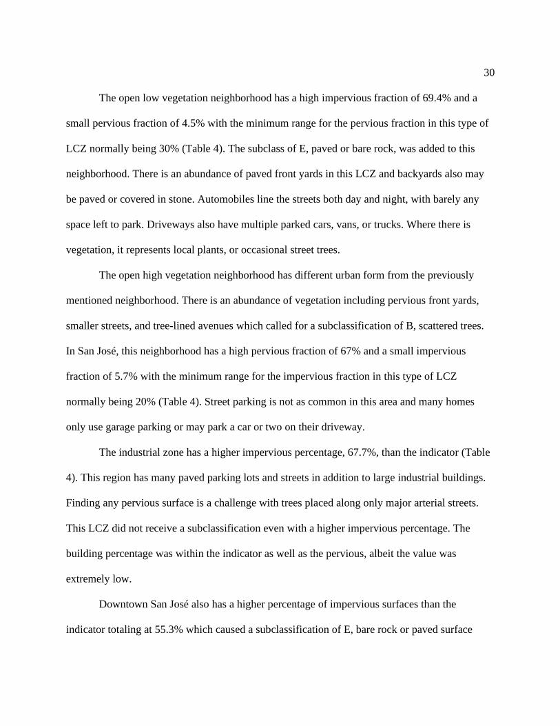
the evenings and 11 of the 15 were different in the afternoon. (Figure 12 & Figure 13). The
complete table of pairwise comparison of LCZs is provided in Appendix A and B.
The lake, which had a temperature departure closest to the mean in the evening samples,
did not differ significantly from either open low rise neighborhood or the industrial LCZ
(P>0.05, Figure 12). The industrial LCZ and open low vegetation neighborhood had high
impervious percentage (67% and 69.4%, respectively) and did not differ significantly from one
another. The downtown and industry LCZs were not significantly different from one another
(P>0.53), which have similar building fraction percentages and high impervious percentages.
In the evenings, there were significantly different evening temperatures in the open
vegetation neighborhoods, which also differed in pervious fractions with the open high
vegetation neighborhood having 62.5% more pervious ground surface. The open low vegetation
neighborhood was warmer than the open high vegetation neighborhood by 0.5 °C and this
difference was significant (P<0.008). The evening temperature of the urban park was
significantly different from all sites with the lowest temperatures in the evenings among all six
LCZs (P<0.05). The open high vegetation neighborhood was 0.5 °C warmer than the park
(P<0.002) while the open low rise was 1 °C warmer than the park (P<0.0001).
The downtown midrise LCZ was warmer than the urban park by 1.5 °C, and this
difference was significant (P<0.0001). Furthermore, the downtown midrise LCZ had the highest
38
temperatures and the urban park produced the coolest temperatures below the transect mean.
These two LCZ had the largest temperature difference between any two LCZs.
Figure 12: Box plots for each sampled LCZ showing the distribution of temperature variability
for 13 evening transects with the wind direction from the North to Northwest. The LCZ average
transect median (red line) is inside of the box. The top of the blue box represents the 75th
percentile and the bottom represents the 25th percentile. The black lines extending from the
boxes represent the tails of the temperature distribution and the red marks represent outliers.
In the afternoons, the open low vegetation neighborhood had a temperature departure
closest to the mean and was not significantly different from the industry, downtown, or open
high vegetation neighborhood. The industry LCZ was not significantly different than the open
high vegetation neighborhood during the afternoon transects (P<0.04). The downtown midrise
was the second coolest LCZ and was 0.9 °C cooler than the light industry LCZ, and this
difference was significant (P<0.012).
Unlike in the evenings, the Lake afternoon temperature was statistically lower than all
other LCZs. The afternoon lake temperature was 1.4 °C below the transect mean. The urban park

39
had the warmest afternoon temperature and was significantly different from all other LCZs in the
afternoons such as the downtown LCZ which was 1.9 °C cooler (P<0.0001). The lake was 2.9 °C
cooler than the urban park, and this difference was significant (P<0.0001).
Figure 13: Box plots for each sampled LCZ showing the distribution of temperature variability
for all five afternoon transects with the wind direction from the North to Northwest. The LCZ
average transect median (red line) is inside of the box. The top of the blue box represents the
75th percentile and the bottom represents the 25th percentile. The black lines extending from the
boxes represent the tails of the temperature distribution and the red marks represent outliers.
3.5 Comparing Wind Speed in the Evenings
Theoretically, UHI is strongest on calm evenings due to the decrease in advection and
turbulent wind activity as weak winds and cloudless skies create the ideal conditions to trap heat
in microclimates (Oke 1978). To examine windspeed, transects with windspeeds greater than the
average of all evening transects were categorized as ‘windier’ evenings. Similarly, windspeeds

40
less than all evening transect wind speed mean were categorized as ‘less windy’ evenings.
Average temperature departures for windier transects (4.1 m s-1) are compared with less windy
transects (2.6 m s-1) in Figure 14.
Figure 14: Mean temperature departure for 13 evening transects on 6 windier evenings and 7 less
windy evenings. The site temperature mean was obtained for the 13 evening transects surveyed
with North to Northwest wind direction. The average wind speed was 3.29 m s-1. The average
wind speed for windier evenings was 4.1 m s-1 and for less windy evenings, 2.6 m s-1.
The patterns of temperature differences between sites remained similar to each other and
those for the complete dataset in the evening with the downtown midrise showing the highest
positive value and the urban park the coolest temperatures. The main difference appears to be
that the temperature differences are enhanced under lower wind speeds. For example, the
difference between downtown and the urban park was 1.19 °C under windier conditions and
climbed to 1.75 °C under weaker winds.

41
Windier conditions weakened temperatures differences. The lake warmed on less windy
evenings at 0.1 °C above the transect mean and showed a temperature departure of 0.03 °C
below the average on windier evenings (Figure 14). On windier evenings, the difference between
the open low vegetation neighborhood and the open high vegetation neighborhood was 0.3 °C
while on less windy evenings, this difference was greater at 0.44 °C. The industry LCZ warmed
from 0.33 °C to 0.45 °C on less windy evenings, an increase of 0.12 (Figure 14).
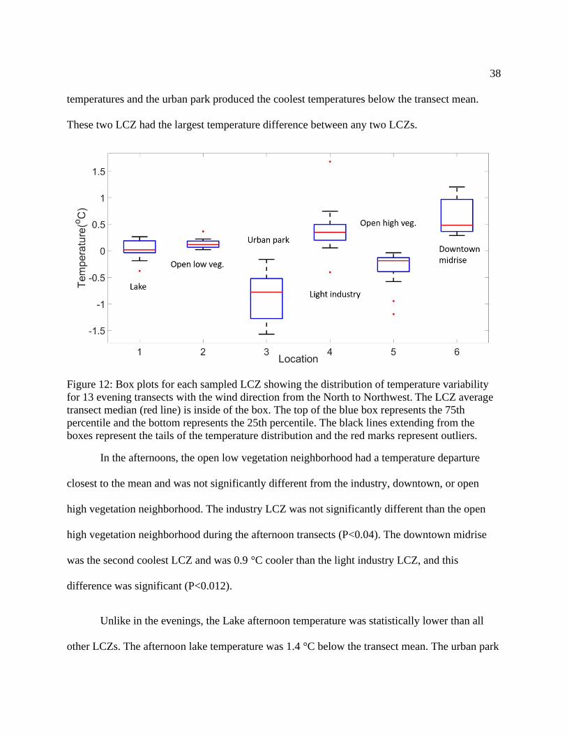
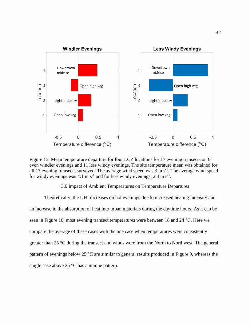
Without consideration for wind direction, Figure 15 shows the same pattern of weaker
temperature differences during windier evenings. The temperature difference decreases between
the open low vegetation and high vegetation neighborhoods on windier evenings with a
difference of 0.3 °C. On less windy evenings, the temperature difference is increased to 0.71 °C
between neighborhoods (Figure 15). The warming in the downtown midrise zone was almost
double on less windy evenings, at 0.87 °C, while at 0.48 °C on windier evenings (Figure 15).
The industry LCZ barely changed temperatures under varying wind conditions,
decreasing by 0.03 °C, from 0.36 °C on less windy evenings to 0.33 °C on windier evenings
(Figure 15). However, the open high vegetation neighborhood has the same pattern as Figure 14
with an increased departure at 0.6 °C on less windy evenings and a weakened departure on
windier evenings at 0.18 °C (Figure 15).
42
Figure 15: Mean temperature departure for four LCZ locations for 17 evening transects on 6
even windier evenings and 11 less windy evenings. The site temperature mean was obtained for
all 17 evening transects surveyed. The average wind speed was 3 m s-1. The average wind speed
for windy evenings was 4.1 m s-1 and for less windy evenings, 2.4 m s-1.
3.6 Impact of Ambient Temperatures on Temperature Departures
Theoretically, the UHI increases on hot evenings due to increased heating intensity and
an increase in the absorption of heat into urban materials during the daytime hours. As it can be
seen in Figure 16, most evening transect temperatures were between 18 and 24 °C. Here we
compare the average of these cases with the one case when temperatures were consistently
greater than 25 °C during the transect and winds were from the North to Northwest. The general
pattern of evenings below 25 °C are similar to general results produced in Figure 9, whereas the
single case above 25 °C has a unique pattern.

43
Figure 16: Mean temperature departure for each LCZ location on evenings with average
temperature above or below 25 °C. The site mean was obtained from temperature transects with
a wind direction from the North or Northwest. The mean transect temperature for the transect
above 25 °C was 32.2 °C and on evenings below 25 °C the mean was 20.8 °C.
Temperature differences were strengthened in only two LCZs, the downtown midrise and
open high vegetation neighborhood, under hotter background conditions. The downtown midrise
zone increased in temperature by 0.4 °C and the open high vegetation neighborhood showed an
additional 0.3 °C departure from 0.3 °C to 0.6 °C on the warm evening. The downtown was 1.6
°C hotter than the open high vegetation neighborhood on the evening above 25 °C, but only 0.9
°C hotter when temperatures were below 25 °C.
Temperature departures from the average weakened in the open low vegetation
neighborhood, industry, and urban park on the evening above 25 °C. There is a low positive
temperature departure in the urban park when temperatures are above 25 °C at 0.16 °C. On
44
evenings below 25 °C, the urban park had a strong temperature departure at 0.93 °C, which is
0.77 °C cooler than on the evening above 25 °C. The industry zone gained 0.37 °C on evenings
below 25 °C and the low vegetation neighborhood was strengthened as well, but only 0.08 °C on
evenings below 25 °C. The lake experienced a little warming on evenings below 25 °C of only
0.07 °C while on the evening above 25 °C, the lake was 0.38 °C cooler than the average city
temperature.
Excluding wind directions from the north to northwest, there were 3 transects with
average transect temperature above 25 °C and 14 transects below 25 °C (Figure 17). These four
LCZs follow similar patterns to the general results in Figure 9, with the downtown midrise being
the warmest LCZ. Three LCZs, open high vegetation neighborhood, industry, and downtown
midrise, had strengthened temperature departures under hotter background conditions.
Figure 17: Mean temperature departure for four LCZ location on evenings with average
temperature above or below 25 °C. The site mean was obtained from all 17 transects with all

45
wind directions. The mean transect temperature for evenings above 25 °C was 30.7 °C and on
evenings below 25 °C the mean was 20.3 °C.
The downtown midrise zone saw the largest increase in warming by 0.45 °C to 1.1 °C on
the evening over 25 °C and was 2.2 °C hotter than the open high vegetation neighborhood on
evenings above 25 °C (Figure 17). On evenings below 25 °C, the difference was weakened to
0.96 °C. The light industry zone saw a minimal increase in warming of 0.01 °C on the evening
above 25 °C (Figure 17).
The open low vegetation had a negligible change, but it experienced a slight decrease in
temperature, 0.1 °C, on the evenings above 25 °C instead of the strengthened conditions seen in
the other three LCZs (Figure 17). However, the temperature difference between the open low
vegetation neighborhood and open high vegetation neighborhood was 1.13 °C hotter than on
evenings above 25 °C and 0.44 °C hotter on evenings below 25 °C showing strengthened
temperature differences under hotter background conditions.
3.7 Diurnal Variations in Temperature Departure
Two Saturdays in late July were surveyed three times per day to capture the diurnal
variation in temperature across the LCZs. The winds were from the south for both morning
transects, not allowing us to capture the lake and the park accurately. Therefore, analysis was
conducted of the four LCZs which did not require North to Northwest winds for accurate
temperature representation (Figure 18 & Figure 19). As with previous cases of four LCZs, the
mean is derived from the total of all six LCZs.

46
Figure 18: Diurnal temperature distribution for four LCZ on July 21, 2019.
Figure 19: Diurnal temperature distribution for each LCZ on July 27, 2019.

47
The only LCZ to repeat the same pattern on both days is the downtown midrise. On July
21, this LCZ cools in the afternoon, returning to warm temperatures for the morning and evening
(Figure 18). Similarly, on July 27, the same pattern is seen in the downtown LCZ. This is
consistent with the cool temperature departure seen in Figure 10, of about 0.6 °C.
The open high vegetation LCZ has been consistently cool in all previous analysis. On
July 21, the open high vegetation neighborhood experienced cool temperatures during all three
measurement sessions, while the remaining three LCZs varied depending on time of day (Figure
18). However, unlike on July 21, on July 27 the open high vegetation neighborhood experienced
warmer temperatures at 1300 hours but was below the city average for the remaining time slots
(Figure 19).
Warm afternoon temperatures were discovered in Figure 10, which showed on average
this LCZ is about 0.2 °C warmer than the transect mean in the afternoon. The open low
vegetation neighborhood has warm temperature departures on the morning of July 21, but cool
temperatures departures on July 27. It also has cool temperatures in the afternoon of July 21, but
warm temperatures in the afternoon of July 27. Our results from Figure 10 show that this LCZ
temperature departure is on average +0.16 °C, which could explain the slight variation to a
cooler afternoon as it ranges close to the city average.
Discussion
The following is the ranking of LCZs from hottest to coolest LCZ in San José during the
hours just after sunset: Downtown, Industry, Open Low Vegetation Neighborhood, Lake, Open
48
High Vegetation Neighborhood, Urban Park. The only analysis under which this order changed
was the warm transect over 25 °C where the urban park was warmer than the lake and the open
high vegetation neighborhood. The lake LCZ was most similar to the average temperature of the
city.
Our results supported our hypothesis that higher temperatures would occur in the
minimally vegetated neighborhood compared to the highly vegetated neighborhood regardless of
similar urban form. This temperature difference is due to increased evapotranspiration and
pervious ground surface. The pervious fraction in the high vegetation neighborhood was 62.5%
more than in the low vegetation neighborhood and the latter was on average 0.5 °C hotter than
the highly vegetated neighborhood.
Our results also supported the hypothesis that the highly vegetated neighborhood is
expected to have cooler temperatures than other types of built urban form due to the high
pervious ground fraction and vegetation density within this LCZ. This LCZ was the second
coolest LCZ in San José and coolest of the built urban form.
Additionally, our results supported our hypothesis that the highest overall temperature in
the city was expected to be produced by the densely built urban form of the downtown region,
which was 0.6 °C above the transect mean (Figure 9). This LCZ has more buildings and surface
area, a low pervious fraction, a high aspect ratio, and replaced the natural landscape, all of which
causes increases in temperature.
Our results also showed that temperature differences were weakened during windier
conditions due to increased mixing of air between LCZs (Figure 14 & Figure 15). However,
temperature differences were not always strengthened under hotter background conditions.

49
Many general patterns observed in San José were consistent with findings in other urban
climate studies (Yang et al., 2017), showing increased temperatures in dense and built urban
forms and decreased temperatures in areas with higher vegetation or parklands (Spronken-Smith
& Oke, 1998; Jansson et al., 2007; Bottyán et al., 2005; Szeged & Gyarmati 2009).
4.1 Local Climate Zone Classifications
In San José, the subclassification of E, bare rock or paved, was applied to four out of the
six climate zones. Considering the lack of Csb climate representation in LCZ literature and the
cultural and regional construction of San José, there is a pattern of increased paved surfaces
which currently have no comparison. As suggested by Betchel et al. (2015), supervised LCZ
design should be conducted with a local expert so that surface characteristics are incorporated
and considered.
The industrial LCZ did not receive a subclassification even with an increased impervious
fraction. A subclassification of E, bare rock or paved, would be repetitious as the primary land
cover for LCZ 8 is already bare rock or paved. However, in Colombo, Sri Lanka, LCZ 8 was
subclassified with E (Perera & Emmanuel, 2018). Without access to the LCZ measurement data
or sufficient discussion on this particular decision, it is difficult to ascertain the intention behind
this subclassification. Additionally, the framework suggests subclasses for LCZs which feature
alternative urban forms to the parent classification and is not inherently clear if this situation
would require a subclass.
The open low rise neighborhoods in San José did receive separate subclassifications of
either B, for scattered trees, or E, for bare rock or paved. In Vancouver, British Colombia,
Aminipouri et al. (2019), classified a LCZ 6A, similar to San José’s LCZ 6B. This

50
subclassification was prompted by terrain roughness class above the indicator (Aminipouri et al.,
2018). In Nancy, France, LCZ 6 was subclassified with LCZ 9, sparsely built, to account for
values which bordered between LCZ 6 and 9, such as a wider canyon aspect ratio and a
decreased building surface fraction (Leconte et al., 2015). While the canyon aspect ratio in our
LCZ 6s’ are smaller than expected, the building percentage is not below the threshold of 20%.
In downtown San José, a subclassification of 1, high rise, and E, bare rock or paved was
added to account for values outside of the indicators. Similarly, in Nanjing, China, a subclass of
E was added to a LCZ 2 due to an increased impervious fraction of 61% (Yang et al., 2017).
Subclassifications based on the mixing of building heights are common in studies such as in
Londrina, Brazil, which found different combinations of compact LCZs 1,2, and 3 (Anjos et al.,
2020).
Combinations of natural land cover types are not as common and the most comparable
subclassification to San José is seen in Londrina, Brazil, which has a similar subclassification of
LCZ GA for dense trees (Anjos et al., 2020). Subclassification of E, bare rock or paved, was not
found in this literature review for any of the three plant types: low plants, scattered trees, or
dense trees. Even in Colombo, Sri Lanka, where 46 subclasses were assigned, there were no
subclasses assigned to natural landscapes A-G (Perera & Emmanuel, 2018).
In this study, five out of ten LCZ indicators were explored: aspect ratio, building surface
fraction, impervious surface fraction, pervious surface fraction, and height of roughness
elements. Further confidence in the LCZ classification framework would need additional GIS
analysis. Further research would consist of continued investigation and analysis of LCZ
51
geometric surface cover properties and thermal, radiative, and metabolic processes listed in
Table 1.
4.2 Park and Lake Cool Island Effects
Vegetated areas in LCZ research vary depending on eco region. Commonly surveyed
LCZs include dense trees (A), scattered trees (B), and low plants (D). The PCI effect has been
studied at length in conjunction with the growth of UHI research; expected results due to the PCI
phenomena in both the framework and the hypothesis for this study included cooler temperatures
in LCZ B, scattered trees, and the highly vegetated open low rise neighborhood LCZ 6B (Stewart
et al., 2012). The PCI effect for San José is 1.5 °C which is the temperature difference in the
evenings between downtown, LCZ 21E and the urban park, LCZ BE. This PCI difference shows
that areas with more vegetation and soil, such as LCZ BE cooling faster and more effectively
than the built urban surfaces which retain heat cool.
According to theory, evapotranspiration causes cooler temperatures compared to the built
urban form which reduces the amount of vegetation and soil water storage. The urban park, LCZ
BE, did have the coolest temperatures in San José in the evening with an average temperature
departure of 0.9 °C below the average due to vegetation fraction. Similarly, B, scattered trees, or
A, dense trees, were found to be the coolest in Las Vegas, NV, Opelika, AL, Nanjing, China, and
in Vancouver, BC (Stewart & Oke, 2012; Yang et al., 2017; Chieppa et al., 2018; Wang et al.,
2018). LCZ D, low plants, was found to be the coolest vegetated LCZ in three studies, Dublin,
Ireland, Phoenix, AZ, and Londrina, Brazil (Alexander & Mills, 2014; Wang et al., 2018; Anjos
et al., 2020). Consistent with literature (Spronken-Smith & Oke, 1998; Jansson et al., 2007;

52
Bowler et al., 2012) and surface energy balance theory, vegetation provides a cool microclimate
and is an option to combat urban heating.
Afternoon or daytime temperatures were provided for LCZ B in Phoenix, AZ, Las Vegas,
NV, and both cities in Alabama. Unlike San José, all four cities saw cooler temperatures in LCZ
B, below the average (Chieppa et al., 2018; Wang et al., 2018). Theoretically, LCZ B should
have cooler temperatures however, it is possible that due to being a Mediterranean climate with
less than 3% of precipitation falling in the summer months, that there is a lack of water
availability. The lack of water availability during the daytime would hinder evapotranspiration
and plants may have adapted to this climate and close their stoma to preserve energy during hot
afternoons.
In the evenings, LCZ G, water, has the ability to be the coolest LCZ as seen in Las
Vegas, NV with a 5 °C cooling from the average and in Londrina Brazil at 0.8 °C below the city
average (Wang et al., 2018; Anjos et al., 2020). However, in Phoenix, AZ and Auburn, AL,
LCZs with trees were as cool as or cooler than waterbodies (Chieppa et al., 2018; Wang et al.,
2018). Similarly, in San José, the lake was not the coolest LCZ in the evenings, rather the urban
park and highly vegetated neighborhood.
In San José, the lake, LCZ, produced a small positive temperature departure from the
average in the evenings, similar to the lake in Las Vegas which produced a night temperature
departure of 0.4 °C (Wang et al., 2018). This is counterintuitive to the energy budget since it is
expected the lake surface would be dominated by QE and help cool the surrounding area, due to
lower QH. Due to the lake size in San José, small and shallow, it is likely that this lake absorbed

53
heat during the day and is slightly slower to cool than the surrounding surface area during the
evenings, which would explain the result of a small positive temperature departure in Figure 9.
Wang et al. (2018) reported daytime temperature differences for LCZ G in Las Vegas and
Phoenix. Similar to San José, daytime water measurements were the coolest in Phoenix and Las
Vegas (Wang et al., 2018). In Phoenix, LCZ G had a pervious surface fraction of 93% and a
temperature departure of 20 °C below the average (Wang et al., 2018). San José’s afternoon
temperature departure of LCZ G was only 1.5 °C most likely due to a smaller pervious surface
fraction of 79% which also included ground and trees. Water absorbs heat throughout the day
and has a high specific heat capacity, which causes the lake to take a longer time to warm than
paved or ground surfaces. This would explain the cool temperature departures of water bodies
during the daytime when QE is more prominent due to incoming Q* as available energy and
show that LCZ G could be a significant LCZ for people to find respite from daytime heat.
Overall, only two studies showed temperature deviations below the average in LCZ 6, in
Phoenix, AZ with a negligible cooling of 0.1 °C and Vancouver, BC with a cooling of 0.4 K
(Stewart & Oke, 2012; Wang et al., 2018). Neither of these locations had subclassifications. As
expected, the highly vegetated open low rise neighborhood in San José showed cooling similar to
land cover types A or B, rather than built forms reported in Table 2 due to evapotranspiration and
increased water infiltration due to an abundance of pervious surface. Vegetation as a cooling
factor has been addressed widely in the literature (Shashua-Bar & Hoffman, 2000; Bowler et al.,
2012; Gunawardena et al., 2017) and this neighborhood in San José shows a measurable impact
of vegetation to combat urban heating.
54
4.3 The Built Urban Form and UHI
Downtown San José has the highest average temperature departure in the evenings in
agreement with theory and previous studies (e.g. Table 2) which show the increase of urban
materials and the replacement of the natural landscape causes an increase in temperature. These
increases in the built urban form lead to increased temperatures and the UHI from the absorption
of additional heat which is penetrated into the urban materials during the day which alters the
SEB (Oke, 1987). Downtown is the densest LCZ in San José and has the largest surface area,
largest impervious fraction, and is able to absorb more heat than smaller buildings. Likewise,
LCZs 1 and 2 report the most warming or highest UHI intensity in every study surveyed that
reported compact high rise or midrise LCZs (Table 2). Londrina, Brazil produced the same
warming as San José (0.6 °C) for compact midrise urban form (Anjos et al., 2020). In Dublin,
Ireland, LCZ 2 reported a 2.1 °C temperature departure above the average and was the hottest
LCZ in the study (Alexander & Mills, 2014). In Kochi, India, the compact midrise LCZ was 2.8
°C warmer than the lightweight low rise zone (Thomas et al., 2014).
Downtown is consistently the coolest LCZ in the afternoon (Figure 13). According to
UHI literature, increases in density of buildings and increases of the built urban form lead to the
UHI especially in the evenings, but also in the afternoons in highly urbanized areas or urban
centers (Gedzelman et al., 2003; Giridharan et al., 2004). This LCZ was expected to be above the
city average and we are unable to fully explain the consistent negative temperature departure in
this LCZ. Possible reasons include this LCZ being the northmost location with winds blowing
from the Bay across the airport cooling the downtown region more effectively than the
neighborhoods sampled to the south. Another possibility is shading caused by multistory

55
buildings coupled with the absorption of incoming radiation into urban materials or increased
surface roughness due to a mix of building heights from midrise to high rise. Additional
afternoon temperature samples would be required to further investigate this pattern. Absorption
of incoming Q* during the day does lead to the fact that this LCZ had the highest temperatures at
night due to the release of the stored heat from the day.
The industry zone has higher temperatures in the evenings than most other LCZs due to
large impervious fraction, building surface fraction, and building area. Only LCZ 2 in San José,
downtown midrise, had a larger temperature departure due to an increase in building density and
stories. Building surface area, fraction, and impervious fraction increase temperature due to the
replacement of the natural environment and changes in the SEB due the increase of urban
materials which absorb heat during the day and release it in the evening (Oke, 1987). LCZ 8s
consistently produce second highest temperature departures following compact high rise or
compact midrise LCZs (Table 2). Studies which did not report LCZ 1 or 2, such as Wang et al.
(2018), show large low rise as the hottest LCZs. In Las Vegas, NV and Phoenix AZ, LCZ 8 was
around 1 °C above the city average (Wang et al., 2018). Similar to San José, Londrina, Brazil
showed a temperature departure of 0.4 °C above the average in LCZ 8 (Anjos et al., 2020). In
Chongqing, China, LCZ 8 was 0.7 °C cooler than LCZ 1 (Wang et al., 2017).
The industrial LCZ was similar to its evening departure in the afternoons. Even with
increased building surface area and paved surfaces throughout this LCZ, there are still large gaps
between buildings with an aspect ratio of 0.17 compared to downtown's 0.76. This allows for
greater release of heat at night in the industrial area compared to the more compact downtown.

56
Temperatures in LCZ 6 are, on average, cooler than those in LCZ 2 or 8 which is
comparably seen in Dublin, Ireland where temperatures in LCZ 6 were 1.13 °C cooler than in
LCZ 2, close to San José’s LCZ 6B and LCZ 21E (Alexander & Mills, 2014). LCZ 6 replaces
some of the natural landscape with built environment, but on average, LCZ 6 has smaller
building surface fractions, building surface area, and impervious fractions than LCZ 2 or 8. LCZ
6 usually has higher vegetation fractions than LCZ 2 or 8 and smaller aspect ratios. In agreement
with theory, LCZ 6 in San José was cooler than 2 and 8, due to smaller building surface fractions
and decreased building surface area which cannot absorb as much incoming radiation as other
LCZs with increased amounts of built urban form (Oke, 1987).
Reported temperature departures in LCZ 6 were as high as 1.92 °C in Kochi, India or can
be below the average such as seen in Vancouver, BC with a cooling of 0.4 K which is most
similar to San José LCZ 6B (Stewart & Oke, 2012; Thomas et al., 2014). The open low-rise
classification is meant to have an abundance of pervious land cover in addition to building
materials and concrete (Stewart & Oke, 2012). Therefore, temperature differences or UHI
intensities from the city average are not as large as LCZs 1, 2, or 8 which have buildings with
larger surface area and increased impervious surface fraction.
Open low-rise neighborhoods vary in the studies surveyed. Most LCZ 6 were found to be
warmer than average temperatures or have a positive UHI intensity, such as in Las Vegas, NV
and Auburn, AL at 0.3 °C which was the same as LCZ 6E in San José (Chieppa et al., 2018;
Wang et al., 2018). LCZ 6E produced warmer temperatures than LCZ 6B due to vegetation
differences. Because of this, increasing vegetation in urban areas has been noted as an effective
practice to mitigate the UHI (Bowler et al., 2012; Gunawardena et al., 2017).
57
In Dublin, LCZ 6 had a temperature difference of 0.97 °C above the average, unlike LCZ
6B, while the LCZ 2 had a temperature above the average at 2.1 °C (Alexander & Mills, 2014). In
Kochi, India and Nancy, France, the open low rise LCZs were both nearly 2 °C cooler than the
compact midrise LCZs (Thomas et al., 2014; Leconte et al., 2015). These locations in France and
India come from different climates and yet still have similar temperature differences, showing
support for the universal nature of the LCZ classification system.
The increased impervious fraction in LCZ 6E, the open low vegetation neighborhood,
caused this LCZ to have similar temperatures to the LCZ 8, industry. These LCZs were not
statistically significantly different from each other in San José most likely due to high
impervious percentage in both LCZs (Table 4). In Las Vegas, LCZ 6 had a similar temperature
departure to LCZ 6E in San José of 0.3 °C and was 0.8 °C cooler than LCZ 8 (Wang et al.,
2018). However, the open high vegetation neighborhood, LCZ 6B, was statistically different with
a temperature difference of 0.7 °C, similar to the 0.8 °C in Las Vegas, NV (Wang et al., 2018).
In the daytime, the open high and open low vegetation neighborhoods are similar in
temperature with absorption of heat into building materials occurring during the day. The open
high vegetation neighborhood would have been expected to be lower in temperature due to an
increased amount in vegetation, but like the urban park, both LCZs have temperature departures
above the mean in the afternoons. Possibly, this may be due to a lack of water availability to
support evapotranspiration in a Mediterranean climate like San José or due to the type of plants
in San José and their stomatal reactions to these microclimates.
Our findings that windier conditions produced a decreased range of temperature
departures was similarly seen in Londrina, Brazil, where synoptic patterns were investigated
58
including winds above 4.0 m s-1 (Anjos et al., 2020). Similar to San José, temperature departures
decreased overall, and temperature differences were weaker in Londrina Brazil (Anjos et al.,
2020). Stronger winds produced a temperature difference of 0.5 °C between the lake with dense
trees and compact midrise in Brazil and a 1.2 °C difference between these LCZs with weaker
winds, averaging 2.1m s-1 (Anjos et al., 2020). The likely reason for lower temperature
heterogeneity under windier conditions is caused by the enhancing mixing of air parcels between
neighborhoods.
Conclusions
This study explored the LCZ classification framework as a means to investigate
temperature variation in the built urban form using mobile vehicle measurements in San José,
California. The LCZ framework and subclassification of the built urban form allows for
comparison of LCZs worldwide based on the variation of the built urban form and our results
support LCZ classification as temperature departures are similar in the same built urban forms
from different climates. In San José, densely built urban form, specifically the downtown region,
had the highest temperatures relative to all other LCZs. Results show consistent warm
temperatures in the evenings in the downtown midrise LCZ at 0.6 °C above the transect mean.
The coolest temperatures at 0.9 °C below the transect mean were in the urban park under
typical summer conditions in San José. The urban park was consistently the coolest LCZ with the
open high vegetation neighborhood consistently as the second coolest LCZ. The cooler
temperatures in San José are found in areas which have increased vegetation and increased
pervious surfaces which allow for cooling via evapotranspiration and soil water storage. These
59
areas with additional vegetation and soil produce cooling within the city as seen by our negative
temperature departure of the urban park and open high vegetation neighborhood.
We effectively compared vegetation differences in the open low rise neighborhoods and
demonstrated the importance of vegetation as a cooling component in the built urban form.
Despite their similarity in LCZ characteristics, especially in the built environment, the difference
in pervious fractions showed significant temperature differences between neighborhoods.
Subclassification of these neighborhoods showed similar results to theory based on vegetation
amounts and characteristics of the built urban form where the high vegetation neighborhood
produced a temperature departure below the mean and the low vegetation neighborhood
temperature departure above the mean. With a pervious fraction of 67%, the highly vegetated
single family home neighborhood was on average 0.5 °C cooler than the single family
neighborhood with a pervious fraction of 4.5%.
We found that temperature differences were weakened under windier conditions due to
enhanced mixing caused by winds. Although, temperature differences were not always
strengthened under hotter weather conditions. Unlike the evenings, the diurnal measurements
show different patterns. In the afternoon, the downtown midrise is below the city average
whereas the urban park is the warmest LCZ contrary to their evening patterns. The lake was
consistently around the city average during the evening transects, with the coolest temperatures
midday.
Suggested further exploration would continue GIS investigation to obtain the additional
five geometric, thermal, radiative, and metabolic properties not found in this study. These values

60
would provide more descriptive results of LCZs in San José to allow for further comparison of
LCZs worldwide based on these additional properties.
Future exploration of LCZs in San José should include increased collection of afternoon
temperature data to better explain diurnal patterns and to confirm the unusual downtown cool
island. Additional temperature departure information could be obtained under varying synoptic
conditions such as following rain events, and during different seasons. Additional sampling of
these conditions and time frames would allow for confident and meaningful conclusions since
there were limited samples of afternoon, morning, and hot background conditions and no
sampling was done outside of summer.
Climate change scenario modeling based on projected temperature increases and the
temperature differences of LCZs could be conducted to analyze future predictions of urban
heating based on the built urban form. Evidence from this study suggests that the UHI effect is
exacerbated under hotter background conditions. In addition, satellite imagery could be used to
better inform land use and heating differences across San José and could be compared to the field
measurements obtained during this study.
More neighborhoods in San José could be identified for additional LCZs temperature
surveys such as compact low or midrise condominiums or apartment homes or mixed use
development such as residential and retail. Additional LCZ identification and surveys would
allow for a more complete accounting of San José’s microclimate variability.
This study provides a unique sample of a city in a Mediterranean climate using the LCZ
framework. This study, therefore, added a previously unexplored climate type, Csb, to build on
the global datasets already generated. Combined, these findings are critical to informing city

61
planning and urban design in a changing global climate, particularly with consideration for
human health and thermal comfort.
62
References
Alexander, P. J., & Mills, G. (2014). Local climate classification and Dublin’s urban heat island.
Atmosphere, 5(4), 755–774. https://doi.org/10.3390/atmos5040755
Aminipouri, M., Rayner, D., Lindberg, F., Thorsson, S., Knudby, A. J., Zickfeld, K., Middel, A.,
& Krayenhoff, E. S. (2019). Urban tree planting to maintain outdoor thermal comfort
under climate change: The case of Vancouver’s local climate zones. Building and
Environment, 158(February), 226–236. https://doi.org/10.1016/j.buildenv.2019.05.022
Anjos, M., Targino, A. C., Krecl, P., Oukawa, G. Y., & Braga, R. F. (2020). Analysis of the
urban heat island under different synoptic patterns using local climate zones. Building
and Environment, 185(August). https://doi.org/10.1016/j.buildenv.2020.107268
Bechtel, B., Alexander, P. J., Böhner, J., Ching, J., Conrad, O., Feddema, J., Mills, G., See, L., &
Stewart, I. (2015). Mapping local climate zones for a worldwide database of the form and
function of cities. ISPRS International Journal of Geo-Information, 4(1), 199–219.
https://doi.org/10.3390/ijgi4010199
Bechtel, B., Demuzere, M., Mills, G., Zhan, W., Sismanidis, P., Small, C., & Voogt, J. (2019).
SUHI analysis using Local Climate Zones—A comparison of 50 cities. Urban Climate,
28(January), 100451. https://doi.org/10.1016/j.uclim.2019.01.005
Bechtel, B., Demuzere, M., Sismanidis, P., Fenner, D., Brousse, O., Beck, C., Van Coillie, F.,
Conrad, O., Keramitsoglou, I., Middel, A., Mills, G., Niyogi, D., Otto, M., See, L., &
Verdonck, M.-L. (2017). Quality of Crowdsourced Data on Urban Morphology—The
Human Influence Experiment (HUMINEX). Urban Science, 1(2), 15.
https://doi.org/10.3390/urbansci1020015
Bottyán, Z., Kircsi, A., Szegedi, S., & Unger, J. (2005). The relationship between built-up areas
and the spatial development of the mean maximum urban heat island in Debrecen,
Hungary. International Journal of Climatology, 25(3), 405–418.
https://doi.org/10.1002/joc.1138
Bowler, D. E., Buyung-Ali, L., Knight, T. M., & Pullin, A. S. (2010). Urban greening to cool
towns and cities: A systematic review of the empirical evidence. Landscape and Urban
Planning, 97(3), 147–155. https://doi.org/10.1016/j.landurbplan.2010.05.006
Chieppa, J., Bush, A., & Mitra, C. (2018). Using ‘“Local Climate Zones”’ to detect urban heat
island on two small cities in Alabama. Earth Interactions, 22(16).
https://doi.org/10.1175/EI-D-17-0020.1
Dahl, K., Licker, R., Abatzoglou, J.T., & Declet-Barreto, J. (2019). Increased frequency of and
population exposure to extreme heat index days in the United States during the 21st
century. Environmental Research Communications, 1(7). https://doi.org/10.1088/2515-
7620/ab27cf

63
Demuzere, M., Bechtel, B., & Mills, G. (2019). Global transferability of local climate zone
models. Urban Climate, 27(February 2018), 46–63.
https://doi.org/10.1016/j.uclim.2018.11.001
Department of Planning (2014). Fact Sheet: History and Geography. San José Department of
Planning: Building & Code Enforcement.
http://www.sanjoseca.gov/index.aspx?NID=2044
Gago, E. J., Roldan, J., Pacheco-Torres, R., & Ordóñez, J. (2013). The city and urban heat
islands: A review of strategies to mitigate adverse effects. Renewable and Sustainable
Energy Reviews, 25, 749–758. https://doi.org/10.1016/j.rser.2013.05.057
Gedzelman, S. D., Austin, S., Cermak, R., Stefano, N., Partridge, S., Quesenberry, S., &
Robinson, D. A. (2003). Mesoscale aspects of the Urban Heat Island around New York
City. Theoretical and Applied Climatology, 75(1–2), 29–42.
https://doi.org/10.1007/s00704-002-0724-2
Giridharan, R., Ganesan, S., & Lau, S. S. Y. (2004). Daytime urban heat island effect in high-rise
and high-density residential developments in Hong Kong. Energy and Buildings, 36(6),
525–534. https://doi.org/10.1016/j.enbuild.2003.12.016
Google Earth Pro. 2020.
Grimmond, C. S. B. (2006). Progress in measuring and observing the urban atmosphere.
Theoretical and Applied Climatology, 84(1–3), 3–22. https://doi.org/10.1007/s00704-
005-0140-5
Gunawardena, K. R., Wells, M. J., & Kershaw, T. (2017). Utilising green and bluespace to
mitigate urban heat island intensity. Science of the Total Environment, 584–585, 1040–
1055. https://doi.org/10.1016/j.scitotenv.2017.01.158
Iamarino, M., Beevers, S., & Grimmond, C. S. B. (2012). High-resolution (space, time)
anthropogenic heat emissions: London 1970-2025. International Journal of Climatology,
32(11), 1754–1767. https://doi.org/10.1002/joc.2390
Jansson, C., Jansson, P. E., & Gustafsson, D. (2007). Near surface climate in an urban vegetated
park and its surroundings. Theoretical and Applied Climatology, 89(3–4), 185–193.
https://doi.org/10.1007/s00704-006-0259-z
Kleerekoper, L., Van Esch, M., & Salcedo, T. B. (2012). How to make a city climate-proof,
addressing the urban heat island effect. Resources, Conservation and Recycling, 64, 30–
38. https://doi.org/10.1016/j.resconrec.2011.06.004
Kotharkar, R., & Bagade, A. (2018). Evaluating urban heat island in the critical local climate
zones of an Indian city. Landscape and Urban Planning, 169(August 2017), 92–104.
https://doi.org/10.1016/j.landurbplan.2017.08.009
Leconte, F., Bouyer, J., Claverie, R., & Pétrissans, M. (2015). Using Local Climate Zone scheme
for UHI assessment: Evaluation of the method using mobile measurements. Building and
Environment, 83, 39–49. https://doi.org/10.1016/j.buildenv.2014.05.005

64
Lehnert, M., Geletič, J., Husák, J., & Vysoudil, M. (2015). Urban field classification by “local
climate zones” in a medium-sized Central European city: the case of Olomouc (Czech
Republic). Theoretical and Applied Climatology, 122(3–4), 531–541.
https://doi.org/10.1007/s00704-014-1309-6
Miller, M. (1999). Climate of San José. NOAA Technical Memorandum.
Morgan, D., Myrup, L., Rogers, D., & Baskett, R. (1977). Microclimates within an Urban Area.
Annals of the Association of American Geographers, Mar., 1977, Vol. 67, No. 1.
https://www.jstor.org/stable/2562241
Multi- Resolution Land Characteristics Consortium. 2020. National Land Cover Database
(NLCD) Retrieved October 15, 2020 from
https://www.mrlc.gov/data?f%5B0%5D=category%3ALand%20Cover&f%5B1%5D=cat
egory%3AUrban%20Imperviousness
National Climate Data Center. 2020. National Centers for Environmental Information. National
Oceanic and Atmospheric Administration. Retrieved June 6, 2020 from
https://www.ncdc.noaa.gov/
Norton, B. A., Coutts, A. M., Livesley, S. J., Harris, R. J., Hunter, A. M., & Williams, N. S. G.
(2015). Planning for cooler cities: A framework to prioritise green infrastructure to
mitigate high temperatures in urban landscapes. Landscape and Urban Planning, 134,
127–138. https://doi.org/10.1016/j.landurbplan.2014.10.018
Offerle, B., Grimmond, C. S. B., & Oke, T. R. (2003). Parameterization of net all-wave radiation
for urban areas. Journal of Applied Meteorology, 42(8), 1157–1173.
https://doi.org/10.1175/1520-0450(2003)042<1157:PONARF>2.0.CO;2
Oke, T. R. 1987. Boundary Layer Climates. 2nd Ed. Routledge.
Oke, T. R. (2006). Initial guidance to obtain representative meteorological observations at urban
sites. World Meteorological Organization: Instruments and Observing Methods. 81.
https://doi.org/10.1007/s12028-011-9538-3
Oke, T. R. (1988). The urban energy balance. Progress in Physical Geography, 12(4), 471–508.
https://doi.org/10.1177/030913338801200401
Oke, T. R. (2006). Towards better scientific communication in urban climate. Theoretical and
Applied Climatology, 84(1–3), 179–190. https://doi.org/10.1007/s00704-005-0153-0
Perera, N. G. R., & Emmanuel, R. (2018). A “Local Climate Zone” based approach to urban
planning in Colombo, Sri Lanka. Urban Climate, 23, 188–203.
https://doi.org/10.1016/j.uclim.2016.11.006
Sakakibara, Y., & Matsui, E. (2005). Relation between heat island intensity and city size
indices/urban canopy characteristics in settlements of Nagano basin, Japan. Geographical
Review of Japan, 78(12), 812–824. https://doi.org/10.4157/grj.78.812

65
San José CA GIS Open Data. 2020. Building Footprint. geo.sanjoseca.gov. Retrieved October 1,
2020 from https://gisdata-csj.opendata.arcgis.com/datasets/building-footprint?geometry=-
122.541%2C37.110%2C-121.159%2C37.493
Shashua-Bar, L., & Hoffman, M. E. (2000). Vegetation as a climatic component in the design of
an urban street. Energy and Buildings, 31(3), 221–235. https://doi.org/10.1016/S0378-
7788(99)00018-3
Skarbit, N., Stewart, I. D., Unger, J., & Gál, T. (2017). Employing an urban meteorological
network to monitor air temperature conditions in the ‘local climate zones’ of Szeged,
Hungary. International Journal of Climatology, 37(March), 582–596.
https://doi.org/10.1002/joc.5023
Spronken-Smith, R. A., & Oke, T. R. (1998). The thermal regime of urban parks in two cities
with different summer climates. International Journal of Remote Sensing, 19(11), 2085–
2104. https://doi.org/10.1080/014311698214884
Stevan, S., Dragan, M., Lazar, L., Vladimir, M., Daniela, A., & Dragoslav, P. (2013). Classifying
urban meteorological stations sites by “local climate zones”: Preliminary results for the
City of Novi Sad (Serbia). Geographica Pannonica, 17(3), 60–68.
Stewart, I. D., & Oke, T.R. (2012). Datasheets for Local Climate Zones, 93(12).
https://doi.org/10.1175/BAMS-D-11-00019.2
Stewart, I. D., & Oke, T.R. (2012). Local Climate Zones for Urban Temperature Studies.
American Meteorological Society. JSTOR 93(12), 1879-1900.
Szeged, S., & Gyarmati, R., (2009). Impacts of Urban Green Spaces on the Spatial Structure of
the Urban Heat Island in Debrecen and Different Sized Settlements in its Neighborhood.
Acta Climatologcia Chorologica, 42-43, 151-158.
Terjung, W.H. and Collaborators. (1970). The Energy Balance Climatology of a City-Man
System. Annals of the Association of American Geographers, Sep., 1970 , Vol. 60 , No.
3. https://www.jstor.org/stable/2561671
Terjung W.H., & Louie, S.S. (1973). Solar Radiation and Urban Heat islands. Annals of the
Association of American Geographers, Jun., 1973, Vol. 63, No. 2.
https://www.jstor.org/stable/2562269
Thomas, G., Sherin, A. P., Ansar, S., & Zachariah, E. J. (2014). Analysis of Urban Heat Island in
Kochi, India, Using a Modified Local Climate Zone Classification. Procedia
Environmental Sciences, 21, 3–13. https://doi.org/10.1016/j.proenv.2014.09.002
United Nations. “68% Of the World Population Projected to Live in Urban Areas by 2050, Says
UN | UN DESA Department of Economic and Social Affairs.” United Nations, United
Nations, 16 May 2018, www.un.org/development/desa/en/news/population/2018-
revision-of-world-urbanization-prospects.html.

66
Whitman, S., Good, G., Donoghue, E.R., Benbow, N., Shou, W., & Mou, S., (1997) Morality in
Chicago attributed to the July 1995 heat wave. American Journal of Public Health, 87(9),
1515-1518.
Wang, C., Middel, A., Myint, S. W., Kaplan, S., Brazel, A. J., & Lukasczyk, J. (2018). Assessing
local climate zones in arid cities: The case of Phoenix, Arizona and Las Vegas, Nevada.
ISPRS Journal of Photogrammetry and Remote Sensing, 141, 59–71.
https://doi.org/10.1016/j.isprsjprs.2018.04.009
Wong, N. H., & Yu, C. (2005). Study of green areas and urban heat island in a tropical city.
Habitat International, 29(3), 547–558. https://doi.org/10.1016/j.habitatint.2004.04.008
Xue, J., You, R., Liu, W., Chen, C., & Lai, D. (2020). Applications of local climate zone
classification scheme to improve urban sustainability: A bibliometric review. Sustainability,
12(19), 1–14. https://doi.org/10.3390/su12198083
Yang, X., Yao, L., Zhu, C., Jin, T., & Peng, L. L. (2017). Analysis of Local Heat Islands in
Nanjing, China, based on the Local Climate Zone Scheme. Procedia Engineering, 205,
2501–2508. https://doi.org/10.1016/j.proeng.2017.09.980

67
Appendices
Appendix A: Evening pairwise comparisons of temperature differences between LCZs with P
Values indicating significant or not significant differences between LCZs.
Location Comparison Absolute Temperature
Difference (° C)
P Value
Lake & Open Low Vegetation Neighborhood 0.12 0.9651
Lake & Urban Park 0.9 0.0001
Lake & Industry 0.36 0.1031
Lake & Open High Vegetation Neighborhood 0.37 0.0795
Lake & Downtown 0.59 0.0006
Open Low Vegetation Neighborhood & Urban Park 1.01 0.0001
Open Low Vegetation Neighborhood & Industry 0.25 0.4584
Open Low Vegetation Neighborhood & Open High
Vegetation Neighborhood
0.48 0.0086
Open Low Vegetation Neighborhood & Downtown 0.48 0.0092
Urban Park & Industry 1.26 0.0001
Urban Park & Open High Vegetation Neighborhood 0.53 0.0027
Urban Park & Downtown 1.49 0.0001
Industry & Open High Vegetation Neighborhood 0.73 0.0001
Industry & Downtown 0.23 0.5329
Open High Vegetation Neighborhood & Downtown 0.96 0.0001

68
Appendix B: Afternoon pairwise comparisons of temperature differences between LCZs with P
Values indicating significant or not significant differences between LCZs
Location Comparison Absolute Temperature
Difference (° C)
P Value
Lake & Open Low Vegetation Neighborhood 1.6 0.0001
Lake & Urban Park 2.79 0.0001
Lake & Industry 1.79 0.0001
Lake & Open High Vegetation Neighborhood 1.65 0.0001
Lake & Downtown 0.85 0.0297
Open Low Vegetation Neighborhood & Urban Park 1.17 0.0014
Open Low Vegetation Neighborhood & Industry 0.17 0.9831
Open Low Vegetation Neighborhood & Open High
Vegetation Neighborhood
0.03 0.9999
Open Low Vegetation Neighborhood & Downtown 0.77 0.0564
Urban Park & Industry 1.0 0.0071
Urban Park & Open High Vegetation Neighborhood 1.14 0.0019
Urban Park & Downtown 1.94 0.0001
Industry & Open High Vegetation Neighborhood 0.14 0.9938
Industry & Downtown 0.94 0.0124
Open High Vegetation Neighborhood & Downtown 0.81 0.0423