Impact of the LMDZ atmospheric grid configurationon the climate and sensitivity of the IPSL-CM5A coupled model

Frederic Hourdin • Marie-Alice Foujols • Francis Codron • Virginie Guemas •

Jean-Louis Dufresne • Sandrine Bony • Sebastien Denvil • Lionel Guez •

Francois Lott • Josefine Ghattas • Pascale Braconnot • Olivier Marti •

Yann Meurdesoif • Laurent Bopp

Received: 24 October 2011 / Accepted: 28 May 2012 / Published online: 26 July 2012

� The Author(s) 2012. This article is published with open access at Springerlink.com

Abstract The IPSL-CM5A climate model was used to

perform a large number of control, historical and climate

change simulations in the frame of CMIP5. The refined

horizontal and vertical grid of the atmospheric component,

LMDZ, constitutes a major difference compared to the pre-

vious IPSL-CM4 version used for CMIP3. From imposed-

SST (Sea Surface Temperature) and coupled numerical

experiments, we systematically analyze the impact of the

horizontal and vertical grid resolution on the simulated cli-

mate. The refinement of the horizontal grid results in a sys-

tematic reduction of major biases in the mean tropospheric

structures and SST. The mid-latitude jets, located too close to

the equator with the coarsest grids, move poleward. This

robust feature, is accompanied by a drying at mid-latitudes

and a reduction of cold biases in mid-latitudes relative to the

equator. The model was also extended to the stratosphere by

increasing the number of layers on the vertical from 19 to 39

(15 in the stratosphere) and adding relevant parameteriza-

tions. The 39-layer version captures the dominant modes of

the stratospheric variability and exhibits stratospheric sud-

den warmings. Changing either the vertical or horizontal

resolution modifies the global energy balance in imposed-

SST simulations by typically several W/m2 which translates

in the coupled atmosphere-ocean simulations into a different

global-mean SST. The sensitivity is of about 1.2 K per 1 W/m2

when varying the horizontal grid. A re-tuning of model

parameters was thus required to restore this energy balance

in the imposed-SST simulations and reduce the biases in the

simulated mean surface temperature and, to some extent,

latitudinal SST variations in the coupled experiments for the

modern climate. The tuning hardly compensates, however,

for robust biases of the coupled model. Despite the wide

range of grid configurations explored and their significant

impact on the present-day climate, the climate sensitivity

remains essentially unchanged.

Keywords Climate modeling � Grid resolution �Climate change projections

1 Introduction

Numerical simulations with general circulation models are

at the heart of climate change studies. They are used to

quantify the impact of greenhouse gas increase on the

evolution of the global climate, to unravel the physical

mechanisms that control climate sensitivity, and to verify

theoretical hypotheses or mechanisms while taking into

account the complexity of the climate system. Those

numerical models however still provide only an approxi-

mate representation of the real climate system, which

This paper is a contribution to the special issue on the IPSL and

CNRM global climate and Earth System Models, bothdeveloped in

France and contributing to the 5th coupled model intercomparison

project.

F. Hourdin (&)

Laboratoire de Meteorologie Dynamique, (LMD/IPSL),

CNRS-UPMC-ENS-EP, Tr 45-55, 3e et, B99 Jussieu,

Paris 75005, France

e-mail: hourdin@lmd.jussieu.fr

M.-A. Foujols � S. Denvil � J. Ghattas

Institut Pierre-Simon Laplace (IPSL), CNRS-UPMC,

UVSQ, CEA, Paris, France

F. Codron � V. Guemas � J.-L. Dufresne � S. Bony �L. Guez � F. Lott

LMD, Paris, France

P. Braconnot � O. Marti � Y. Meurdesoif � L. Bopp

Laboratoire des Sciences du Climate et de l’Environnement

(LSCE/IPSL), CNRS-CEA-UVSQ, Saclay, France

123

Clim Dyn (2013) 40:2167–2192

DOI 10.1007/s00382-012-1411-3

constitutes a major source of uncertainty for assessing

future climate changes. Improving the models should

therefore be one of the main drivers of climate research.

Among the limitations often emphasized is the rather

coarse spatial resolution of the models used for long-term

climate change simulations, such as those coordinated by

the Coupled Model Intercomparison Project (CMIP, Meehl

et al. 2007; Taylor et al. 2012). It is partly because of this

coarse resolution that key processes such as convection or

clouds have to be parameterized. Systematic centennial

global simulations with meshes of the order of 50 m, which

would be required to explicitly represent boundary layer

clouds, will not be reachable before at least a couple of

decades. It is however expected that significant improve-

ments can already be achieved by increasing the spatial

resolution of current climate models from a few hundreds

to a few tens of kilometers, both because it allows a better

resolution of the dominant atmospheric large scale

dynamics and because it offers a finer description of sur-

face conditions (orography, land/sea distribution). Among

the expected improvements are a reduction of systematic

biases in temperature, precipitation and winds (Pope and

Stratton 2002; Roeckner et al. 2006; Hack et al. 2006), a

better representation of the regional-scale climate (Wil-

liamson et al. 1995; Kobayashi and Sugi 2004; Navarra

2008; Byrkjedal et al. 2008), and a better representation of

rainfall distributions (Kiehl and Williamson 1991; Deque

et al. 1994). An important question in the frame of climate

change simulations is to know whether the model limita-

tions, and in particular the biases which come from the use

of coarse grids, impact the climate sensitivity, both in a

global sense and in modifications of the climate regimes.

Within the framework of the preparation of the 5th

phase of CMIP (CMIP5, Taylor et al. 2012) at the Institut

Pierre-Simon Laplace (IPSL), a systematic exploration of

the impacts of changes in the atmospheric grid configura-

tion of the LMDZ atmospheric general circulation model

was conducted. The simulations were performed with the

LMDZ4 version (Hourdin et al. 2006), the atmospheric

component of the IPSL Coupled Model IPSL-CM4 (Bra-

connot et al. 2007; Marti et al. 2010) that took part in

CMIP3 (Meehl et al. 2007). The results of this systematic

exploration were used to choose the final configuration

LMDZ5A, the atmospheric component of the IPSL-CM5A

model used for CMIP5. Since we intended to contribute to

CMIP5 with a wide variety of configurations and ensem-

bles of simulations (Dufresne et al., this issue), rather

coarse resolutions were explored.

One major goal of this comparison of different grids was

to understand how model biases evolve with increasing

resolution. It appears that grid refinement affects the

position of the jets, and in turn the mid-latitude cold bias

which was one of the major deficiencies of IPSL-CM4. The

cause of the impact of grid refinement on the jet latitude is

found in large-scale atmospheric dynamics, and was stud-

ied by Guemas and Codron (2011). Here we show that

these changes also affect significantly the biases of the

coupled model, as well as the mean climate equilibrium

temperature.

Research over the last decades have led to an increasing

recognition of the role of the stratosphere in controlling

some aspects of the tropospheric climate. This influence is

related to radiative and chemical effects, but also to

dynamical effects: some modes of stratospheric variability

propagate downward, like the Quasi-Biennial Oscillation

(QBO, Baldwin et al. 2001) in the tropics, and the Arctic

Oscillation (AO, Baldwin and Dunkerton 1999) in the mid

latitudes. When the stratospheric anomalies reach the tro-

popause, they can potentially influence the surface climate,

at least in the mid-latitudes (for the AO effect in the LMDZ

mid-latitudes see for instance Lott et al. 2005; Nikulin and

Lott 2010). In order to take into account the impact of the

stratospheric dynamics and chemistry in the coupled cli-

mate simulations, the LMDZ vertical grid was extended in

the stratosphere, with a resolution close to a previous

stratospheric version of LMDZ4 described by Lott et al.

(2005). After these changes the model can be considered as

a high-top climate model.

The results and discussions of the present paper are

mainly focused on the impact of the configuration changes

on the model biases and climate sensitivity. It is shown in

particular that despite a significant impact on some biases

in the present-day climate, the climate sensitivity is weakly

affected by the changes in grid configuration. Additional

results concerning the impact of changes in grid configu-

ration are discussed in companion papers in the same issue:

the impact of the refinement of the horizontal grid on the

atmospheric variability in the north-Atlantic region is dis-

cussed by Cattiaux et al. and results on the ENSO vari-

ability are shown by Dufresne et al. in an overview paper

of the IPSL-CM5 model.1

The paper is organized as follows. In Sect. 2, the con-

sequences of the model horizontal grid refinement on the

mean climatology and on the latitudinal structure in the

LMDZ4 simulations with imposed SSTs, and in the cou-

pled atmosphere-ocean simulations with IPSL-CM4, are

documented and analyzed. Section 3 is dedicated to the

impact of the vertical extension of the model to the

stratosphere. Finally, we compare in Sect. 4 the mean cli-

mate and the climate sensitivity to an increase in green-

house gases of the configurations of the IPSL coupled

model involved in the CMIP3 and CMIP5 exercises.

1 The drafts of the special issue papers can be found at

http://icmc.ipsl.fr/research/international-projects/cmip5/special-issue-

cmip5.

2168 F. Hourdin et al.

123

2 Refining the horizontal grid in LMDZ4

and IPSL-CM4 simulations

We analyze in this section a series of imposed-SST and

coupled atmosphere-ocean simulations, all done with the

same LMDZ4 atmospheric model, but with varying hori-

zontal grids.

2.1 The LMDZ4 general circulation model

LMDZ is an atmospheric general circulation model

developed at Laboratoire de Meteorologie Dynamique. The

dynamical part of the code is based on a finite-difference

formulation of the primitive equations of meteorology (see

e.g. Sadourny and Laval 1984), discretized on a stretchable

(Z of LMDZ standing for Zoom capability) longitude-lat-

itude Arakawa C-grid.

The physical parameterizations of the LMDZ4 versions

are described by Hourdin et al. (2006). The Morcrette

(1991) scheme is used for radiative transfer. Drag and

lifting effects associated with the subgrid-scale orography

are accounted for according to Lott (1999). Turbulent

transport in the planetary boundary layer is treated as a

vertical diffusion with an eddy diffusivity Kz depending on

the local Richardson number according to Laval et al.

(1981). Up-gradient transport of heat in the convective

boundary layer is ensured by adding a prescribed counter-

gradient term of 1 K/km to the vertical derivative of

potential temperature (Deardorff 1966). In the case of

unstable profiles, a dry convective adjustment is applied.

The surface boundary layer is treated according to Louis

(1979). Deep convection is parameterized using the ‘‘epi-

sodic mixing and buoyancy sorting’’ Emanuel scheme

(Emanuel 1991) which assumes quasi-equilibrium between

the opposite influences of the large-scale forcing of con-

vection and of convective instability. A statistical cloud

scheme is used to predict the clouds properties with a

different treatment for convective clouds (Bony and

Emanuel 2001) and large-scale condensation as explained

by Hourdin et al. (2006).

The IPSL-CM4 simulations made for CMIP3 were

performed with a configuration of LMDZ4 made of 96

points in longitude by 72 in latitude (about 3.75� 9 2.5�)

and 19 layers on the vertical (Marti et al. 2010).

2.2 Sensitivity experiments

Identical changes in horizontal resolution are explored here

in both imposed-SST and coupled atmosphere-ocean sim-

ulations with exactly the same source code for the atmo-

spheric component LMDZ4, using a 19-layer vertical grid

(L19). The dynamical time-step and the time constants for

the horizontal diffusion are the only—necessary—

parameter changes between the different simulations, as

described below. The other components of the system, i.e.

the land surface scheme Orchidee and the oceanic circu-

lation model Nemo, are also strictly identical (those ver-

sions are described by Marti et al. 2010).

In the imposed-SST simulations, seasonally varying

SSTs are imposed as a boundary condition. In practice, a

climatological average of the AMIP SSTs (Hurrell et al.

2008) over the period 1970–2000 is used in order to min-

imize the number of years of simulation required to smooth

out the inter-annual variability. The forced simulations are

run for 10 years.

For the coupled atmosphere-ocean simulations, we show

results of control simulations in which the concentration of

greenhouse gases, the Earth’s orbital parameters and solar

irradiance, and aerosols are kept constant, with same values

as in the imposed-SST experiments. The model is run for

100 years. The control simulations are analyzed after a

spin-up phase so that the global radiative balance is within

1 W/m2 from zero in all the simulations. For the illustra-

tions below, the climatological mean seasonal cycle is

computed from the last 10 years of the simulations.

LMDZ uses for the time integration a leapfrog scheme

with a Matsuno (or forward/backward) step every five

leapfrog time-steps. The time step dt is limited by a CFL

criteria, which varies linearly with the size dxmin of the

smallest grid cell: dt \ dxmin/ C, where the C constant is the

external gravity waves phase speed in the model. In longi-

tude-latitude grids, the longitudinal grid size goes to zero at

the pole. In order to avoid the use of too small time-steps, a

longitudinal filter is applied to the dynamical equations after

latitude /0 = 60� in both hemispheres. For a regular longi-

tude-latitude grid as used here, the minimum scale explicitly

accounted for in x is dxmin ¼ dxmax � cosð/0Þ ¼ dxmax=2,

where dxmax = 2p a/IM is the mesh size in x at the equator,

a = 6,400 km being the Earth radius and IM the number of

grid cells in the longitudinal direction. Poleward of the lat-

itude /0, meteorological fields are filtered so as to retain only

wave lengths longer than dxmin. The grid mesh size in latitude

dy = p a/JM—where JM is the number of points in latitude –

is a constant for a given grid. Finally, the time step is limited

by dt \ (p a/C) min(1/IM,1/JM).

In a longitude-latitude grid, the isotropy of the hori-

zontal grid (dy = dx) cannot be insured everywhere.

The original grid, (IM, JM) = (96, 72), or (dk, d/) =

(3.75�, 2.5�), has a ratio IM/JM = 4/3 chosen so that the

grid is isotropic at close to 45� latitude. This choice yields

dx = 3 dy/2 at the equator; and the time step is limited by

dx at /0. Keeping both the same resolution in longitude and

the same value of /0 = 60�, it is possible to refine further

the resolution in latitude up to JM = IM without reducing

the time step. The grid is then isotropic at 60� latitude, and

dx/dy = 2 at the equator.

IPSL-CM5A: impact of the atmospheric grid configuration 2169

123

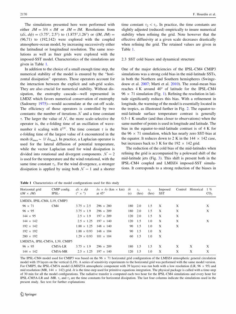
The simulations presented here were performed with

either JM = 3/4 9 IM or JM = IM. Resolutions from

(dk, d/) = (3.75�, 2.5�) to (1.875�,1.26�) or (IM, JM) =

(96,71) to (192,142) were explored with the coupled

atmosphere-ocean model, by increasing successively either

the latitudinal or longitudinal resolution. The same reso-

lutions as well as finer grids were explored with the

imposed-SST model. Characteristics of the simulations are

given in Table 1.

In addition to the choice of a small enough time step, the

numerical stability of the model is ensured by the ‘‘hori-

zontal dissipation’’ operators. Those operators account for

the interaction between the explicit and sub-grid scales.

They are also crucial for numerical stability. Without dis-

sipation, the enstrophy cascade—well represented in

LMDZ which favors numerical conservation of enstrophy

(Sadourny 1975)—would accumulate at the cut-off scale.

The efficiency of those operators is controlled by two

constants: the number of iterations N and a time constant

s. The larger the value of N , the more scale-selective the

operator is, the e-folding time of an oscillation of wave-

number k scaling with k2N . The time constant s is the

e-folding time of the largest value of k encountered in the

mesh (kmax* 1/ dxmin). In practice, a Laplacian operator is

used for the lateral diffusion of potential temperature,

while the vector Laplacian used for wind dissipation is

divided into rotational and divergent components. N ¼ 2

is used for the temperature and the wind rotational, with the

same time constant s1. For the wind divergence, a stronger

dissipation is applied by using both N ¼ 1 and a shorter

time constant s2 \ s1. In practice, the time constants are

slightly adjusted (reduced) empirically to insure numerical

stability when refining the grid. Note however that the

effective diffusivity at a given scale decreases drastically

when refining the grid. The retained values are given in

Table 1.

2.3 SST cold biases and dynamical structure

One of the major deficiencies of the IPSL-CM4 CMIP3

simulations was a strong cold bias in the mid-latitude SSTs,

in both the Northern and Southern hemispheres (Swinge-

douw et al. 2007; Marti et al. 2010). The zonal-mean bias

reaches 4 K around 40� of latitude for the IPSL-CM4

96 9 71 simulation (Fig. 1). Refining the resolution in lati-

tude significantly reduces this bias. With a refinement in

longitude, the warming of the model is essentially located in

the tropics, as illustrated further in Fig. 2. The equator-to-

mid-latitude surface temperature contrast is generally

0.5–1 K smaller (and thus closer to observations) when the

same number of points is used in longitude and latitude. The

bias in the equator-to-mid-latitude contrast is of 4 K for

the 96 9 71 simulation, which has nearly zero SST-bias at

the equator. It reduces down to 2 K in the 144 9 142 case,

but increases back to 3 K for the 192 9 142 grid.

The reduction of the cold bias of the mid-latitudes when

refining the grid is accompanied by a poleward shift of the

mid-latitude jets (Fig. 3). This shift is present both in the

IPSL-CM4 coupled and LMDZ4 imposed-SST simula-

tions. It corresponds to a strong reduction of the biases in

Table 1 Characteristics of the model configurations used for this study

Horizontal grid

(IM 9 JM)

CMIP config.

IPSL-

dk 9 d/(� 9 �)

dx 9 dy (km 9 km)

at 45�dt(s)

s1

(hrs)

s2

(hrs)

Imposed

SST

Control Historical 1 %

CO2

LMDZ4, IPSL-CM4, L19, CMIP3

96 9 71 CM4 3.75 9 2.5 296 9 280 180 2.0 1.5 X X X

96 9 95 3.75 9 1.9 296 9 209 180 2.0 1.5 X X X

144 9 95 2.5 9 1.9 197 9 209 120 2.0 1.5 X X

144 9 142 2.5 9 1.25 197 9 140 120 1.5 1.0 X X X

192 9 142 1.88 9 1.25 148 9 140 90 1.5 1.0 X X

192 9 192 1.88 9 0.93 148 9 104 90 1.5 1.0 X

280 9 192 1.29 9 0.93 101 9 104 60 1.5 1.0 X

LMDZ5A, IPSL-CM5A, L39, CMIP5

96 9 95 CM5A-LR 3.75 9 1.9 296 9 209 180 1.5 1.5 X X X X

144 9 142 CM5A-MR 2.5 9 1.25 197 9 140 120 1.5 1.0 X X X X

The IPSL-CM4 model used for CMIP3 was based on the 96 9 71 horizontal grid configuration of the LMDZ4 atmospheric general circulation

model with 19 layers on the vertical (L19). A series of sensitivity experiments to the horizontal grid was performed with the same model version.

For CMIP5, the IPSL-CM5A model (LMDZ5A atmospheric component with 39 layers) was run both with a low resolution (LR, 96 9 95) and

mid resolution (MR, 144 9 142) grid. dt is the time-step used for primitive equations integration. The physical package is called with a time-step

of 30 min for all the model configurations. The radiative transfer is computed each two hour for the IPSL-CM4 simulations and every hour for

IPSL-CM5A-LR and -MR. s1 and s2 are the time constants for horizontal dissipation. The last four columns indicate the simulations used in the

present study. See text for further explanations

2170 F. Hourdin et al.

123

the representation of the mean zonal wind with grid

refinement, as illustrated in the left column of Fig. 4 for the

imposed-SST simulations. For the coarsest grids, the jets

are shifted toward the equator compared to ERA interim

reanalyzes (as seen from the strong dipole in the zonal

wind bias, centered at the latitude of the jet maximum

intensity).

This jet displacement was studied by Guemas and

Codron (2011) in a set of dynamical core experiments

produced with the LMDZ atmospheric model using the

Held and Suarez (1994) setup. This setup consists in

replacing all the detailed physical parameterizations by a

Newtonian relaxation of the temperature field toward a

zonally-symmetric state, and a Rayleigh (linear) damping of

the low-level wind with an e-folding timescale of 1 day at

the surface. In this configuration, it was shown that the jet

latitude moves poleward when refining the grid in latitude,

and is less affected when increasing the number of grid

points in longitude. It was checked also in this idealized

framework that the changes in jet location when refining the

grid do not come from the use of a shorter time-step.

A similar behavior is found for the imposed-SST and

coupled climate simulations shown here (Fig. 3): a ten-

dency of the jets to move toward the poles when increasing

the resolution, with a stronger impact when refining the

grid in latitude. The effect is not as systematic as in the

idealized dynamical simulations of Guemas and Codron

(2011), which may reflect additional effects due to the

complexity of the climate system.

In order to understand how the grid refinement impacts

the SSTs, i.e. both the increase of the mean temperature

and reduction of the latitudinal contrasts, we start by ana-

lyzing the change in thermodynamical variables and energy

budget in the imposed-SST simulations.

2.4 Thermodynamical variables in the imposed-SST

simulations

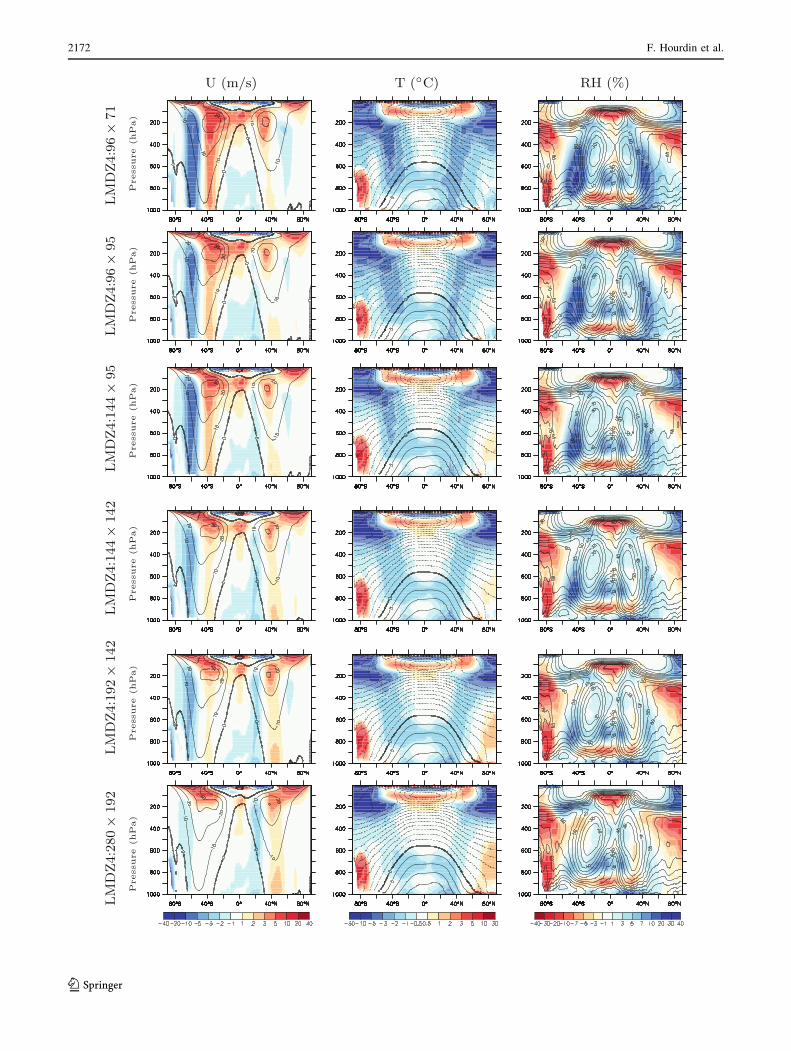
The changes in zonal winds shown in Fig. 4 are accom-

panied by systematic changes in the temperature and

humidity fields.

The mid-latitude tropopause (close to 200 hPa) moistens

when refining the horizontal grid, and becomes too moist

when compared to ERA-Interim for the finest grids. The

tropopause cold bias of the mid to high latitudes also

increases. These two trends are probably related to each

other since the cooling to space, a dominant term of the

radiative balance at this level, is strongly affected by

humidity as already discussed by Hourdin et al. (2006).

Overall, the mid-latitude tropopause is thus too high for the

finest grids explored.

The systematic dry bias of the tropical boundary layer

top (900 hPa) is a direct consequence of an underestimated

moisture vertical transport by the eddy-diffusion parame-

terization used in LMDZ4. It is therefore not affected by

the changes in horizontal resolution.

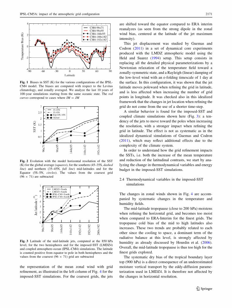
Fig. 1 Biases in SST (K) for the various configurations of the IPSL-

CM4 model. The biases are computed with respect to the Levitus

climatology, and zonally averaged. We analyze the last 10 years of

100-year simulations starting from the same oceanic state. The redcurves correspond to cases where IM = JM

Fig. 2 Evolution with the model horizontal resolution of the SST

(K) for the global average (squares), for the southern (45–35S, dashedline) and northern (35–45N, full line) mid-latitudes and for the

Equator (5S–5N, circles). The values from the coarsest grid

(96 9 71) are subtracted

Fig. 3 Latitude of the mid-latitude jets, computed at the 850 hPa

level, for the two hemispheres and for the imposed-SST (LMDZ4)

and coupled atmosphere-ocean (IPSL-CM4) simulations. The latitude

is counted positive from equator to pole in both hemispheres and the

values from the coarsest (96 9 71) grid are subtracted

IPSL-CM5A: impact of the atmospheric grid configuration 2171

123

2172 F. Hourdin et al.

123

Grid refinement leads to a systematic decrease of the

wet and cold bias of the mid-latitude troposphere. This

decrease of relative humidity is not just a consequence of

the warmer temperature since the specific humidity is

reduced as well, as illustrated in Fig. 5 a and b that show

differences between the 96 9 71 and 144 9 142 grids.

These changes can be interpreted as a shift toward the poles

of the dry anticyclonic regions of the sub-tropics, as seen

from the coincidence of the location of the maximum

drying with that of the maximum latitudinal gradient of

relative humidity (Fig. 5b).

The impact of the poleward displacement of the jet and

of the Hadley-cell boundary is also apparent in the water

budget. The difference of integrated meridional transport of

moisture between the 144 9 142 and 96 9 71 resolutions

is shown on Fig. 6 a (the transport of Lq is shown here

where L is the specific latent heat and q the specific

humidity). The Hadley circulation transports water toward

the equator (more water being transported in the lower

branch of the cell), while the Ferrel Cell and mid-latitude

eddies transport moisture toward the pole. A wider Hadley

cell will thus increase the equatorward transport near the

latitudinal edge of the cell, while the displacement of the

mid-latitude eddies will increase poleward transport in

higher latitudes. The differential transport with increased

resolution is therefore systematically away from the mid-

latitudes (40� N and 40�S) towards the equator and poles.

As a consequence, precipitation is reduced in the mid-

latitudes (Fig. 6 b), even though the evaporation increases

weakly because of the drier atmosphere.

2.5 Energy budget in the imposed-SST simulations

The changes in relative humidity illustrated in Fig. 5b

between resolutions 96 9 71 and 144 9 142 coincide with

large changes in cloud fraction (Fig. 5c). Specifically, the

cloud fraction exhibits a significant decrease near 40� lat-

itude in both hemispheres, and a systematic increase at the

tropopause.

The changes in clouds are associated with pronounced

changes in the Top-of-Atmosphere (TOA) radiative budget

(Fig. 6d). The short-wave (SW) Cloud-Radiative-Forcing

(CRF), defined as the difference of the TOA SW radiation

between all-sky and clear-sky conditions, is strongly

increased in the mid-latitudes, as a consequence of the

decrease of the fractional coverage of low and mid-level

clouds. For long-wave (LW) radiation, the effect of clouds

and the modification of clear-sky radiation partially cancel

each other. The change in SW CRF does not affect sig-

nificantly the atmospheric budget (red curve in Fig. 6c),

since the increase of down-welling SW radiation at surface

(red curve in Fig. 6e) is very close to that at TOA. Con-

versely, the decrease in low-level cloud cover and near

surface humidity in the mid latitudes reduces the LW

(a) Specific humidity : q/qΔ

Δ

Δ

(%)

Pre

ssur

e (h

Pa)

(b) Relative humiditiy : RH (%)

Pre

ssur

e (h

Pa)

(c) Cloud cover : f (%)

Pre

ssur

e (h

Pa)

Fig. 5 Zonal mean change of the latitude-pressure distribution of

moisture and clouds in LMDZ4 imposed-SST simulations associated

with grid refinement from 96 9 71 to 144 9 142: a relative differ-

ence in specific humidity (%), b difference in relative humidity (%)

and c difference in cloud fraction (%). The differences are in colorwhile the contours correspond to the mean value of the 144 9 142

simulation (resp. in g/kg, % and %)

Fig. 4 Ten-year average of the mean meridional structure of the

zonal wind (m/s, left), temperature (�C, middle) and relative humidity

(%, right) for the various imposed-SST simulations with LMDZ4

(L19). The contours correspond to the simulations and the colors to

the difference (bias) with ERAinterim re-analayzes

b

IPSL-CM5A: impact of the atmospheric grid configuration 2173

123

radiation of the atmosphere toward the surface (green

dashed curve in Fig. 6e). The change of net LW radiation

(full green curve) is almost identical to the change in

downweling LW radiation except in the northern mid and

high latitudes where continental surfaces respond to the

increased surface incoming SW radiation.

The sensible heat flux is reduced rather systematically by

about 1 W/m2 due to the warmer atmosphere. The latent heat

is reinforced in the mid latitudes but with a local minimum at

40� latitude. All together, the atmosphere is heated by dia-

batic processes in the mid-latitudes more than in the tropics,

which induces a reduction of the total latitudinal energy

transport (black curve in Fig. 6a). This decrease is however

weak, with a partial compensation between the transport of

Lq and that of the dry static energy CpT ? gz.

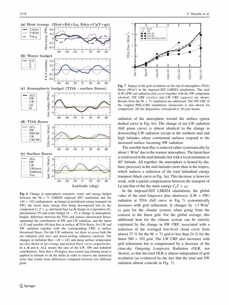
In the imposed-SST LMDZ4 simulations, the global

value of the total longwave plus shortwave (LW ? SW)

radiation at TOA (full curve in Fig. 7) systematically

increases with grid refinement. It changes by ?3 W/m2

(a gain for the climate system) when going from the

coarsest to the finest grid. For the global average, this

additional heat for the climate system can be entirely

explained by the change in SW CRF, associated with a

reduction of the averaged low-level cloud cover from

almost 27 % for the 96 9 71 grid to less than 24 % for the

finest 280 9 192 grid. The LW CRF also increases with

grid refinement but is compensated by a decrease of the

clear-sky Outgoing Longwave Radiation (OLR, not

shown), so that the total OLR is almost independent of grid

resolution (as evidenced by the fact that the total and SW

radiation almost coincide in Fig. 7).

(a)

(b)

(c)

(d)

(e)

Fig. 6 Change in atmospheric transport, water and energy budget

between the 96 9 71 LMDZ4 imposed SST simulation and the

144 9 142 configuration : a change in meridional energy transport (in

PW), the moist static energy Etot being decomposed into its dry

component Cp T ? gz and latent heat Lq; b change in evaporation (E),

precipitation (P) and water budget (E - P); c change in atmospheric

budget, difference between the TOA and surface (downward) fluxes,

separating the contribution of SW and LW radiation, and the latent

(L E) and sensible (H) heat flux at surface; d TOA fluxes, for LW and

SW radiation together with the corresponding CRF; e surface

downward fluxes. For the LW radiation, we show in green both the

net radiation (full line) and down-welling radiation (dashed). The

changes in turbulent flux -(H ? LE) and mean surface temperature

are also shown in (e) (orange and dashed black curves respectively).

In c, d and e, ALL means the sum of the LW, SW and turbulent

contributions. Note that a 20-degree area conserving running mean is

applied in latitude to all the fields in order to remove the numerical

noise that results from differences computed between two different

grids

Fig. 7 Impact of the grid resolution on the top-of-atmosphere (TOA)

fluxes (W/m2) in the imposed-SST LMDZ4 simulations. The total

(LW?SW) net radiation (full curve) together with the SW component

(dashed), SW CRF (circles) and LW CRF (squares) are shown.

Results from the 96 9 71 simulation are subtracted. The SW CRF of

the coupled IPSL-CM4 simulations (diamonds) is also shown for

comparison. All the diagnostics correspond to 10-year means

2174 F. Hourdin et al.

123

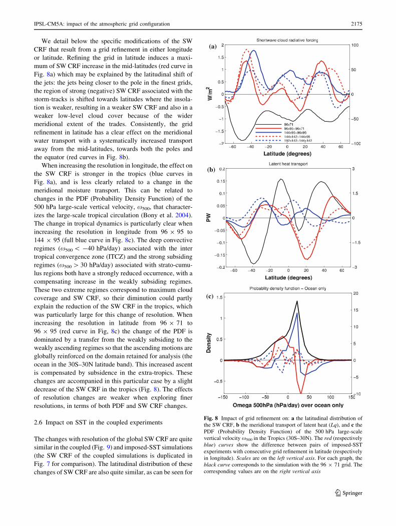
We detail below the specific modifications of the SW

CRF that result from a grid refinement in either longitude

or latitude. Refining the grid in latitude induces a maxi-

mum of SW CRF increase in the mid-latitudes (red curve in

Fig. 8a) which may be explained by the latitudinal shift of

the jets: the jets being closer to the pole in the finest grids,

the region of strong (negative) SW CRF associated with the

storm-tracks is shifted towards latitudes where the insola-

tion is weaker, resulting in a weaker SW CRF and also in a

weaker low-level cloud cover because of the wider

meridional extent of the trades. Consistently, the grid

refinement in latitude has a clear effect on the meridional

water transport with a systematically increased transport

away from the mid-latitudes, towards both the poles and

the equator (red curves in Fig. 8b).

When increasing the resolution in longitude, the effect on

the SW CRF is stronger in the tropics (blue curves in

Fig. 8a), and is less clearly related to a change in the

meridional moisture transport. This can be related to

changes in the PDF (Probability Density Function) of the

500 hPa large-scale vertical velocity, x500, that character-

izes the large-scale tropical circulation (Bony et al. 2004).

The change in tropical dynamics is particularly clear when

increasing the resolution in longitude from 96 9 95 to

144 9 95 (full blue curve in Fig. 8c). The deep convective

regimes (x500 \ -40 hPa/day) associated with the inter

tropical convergence zone (ITCZ) and the strong subsiding

regimes (x500 [ 30 hPa/day) associated with strato-cumu-

lus regions both have a strongly reduced occurrence, with a

compensating increase in the weakly subsiding regimes.

These two extreme regimes correspond to maximum cloud

coverage and SW CRF, so their diminution could partly

explain the reduction of the SW CRF in the tropics, which

was particularly large for this change of resolution. When

increasing the resolution in latitude from 96 9 71 to

96 9 95 (red curve in Fig, 8c) the change of the PDF is

dominated by a transfer from the weakly subsiding to the

weakly ascending regimes so that the ascending motions are

globally reinforced on the domain retained for analysis (the

ocean in the 30S–30N latitude band). This increased ascent

is compensated by subsidence in the extra-tropics. These

changes are accompanied in this particular case by a slight

decrease of the SW CRF in the tropics (Fig. 8). The effects

of resolution changes are weaker when exploring finer

resolutions, in terms of both PDF and SW CRF changes.

2.6 Impact on SST in the coupled experiments

The changes with resolution of the global SW CRF are quite

similar in the coupled (Fig. 9) and imposed-SST simulations

(the SW CRF of the coupled simulations is duplicated in

Fig. 7 for comparison). The latitudinal distribution of these

changes of SW CRF are also quite similar, as can be seen for

(a)

(b)

(c)

Fig. 8 Impact of grid refinement on: a the latitudinal distribution of

the SW CRF, b the meridional transport of latent heat (Lq), and c the

PDF (Probability Density Function) of the 500 hPa large-scale

vertical velocity x500 in the Tropics (30S–30N). The red (respectively

blue) curves show the difference between pairs of imposed-SST

experiments with consecutive grid refinement in latitude (respectively

in longitude). Scales are on the left vertical axis. For each graph, the

black curve corresponds to the simulation with the 96 9 71 grid. The

corresponding values are on the right vertical axis

IPSL-CM5A: impact of the atmospheric grid configuration 2175

123

resolutions 96 9 71 and 144 9 142 by comparing the

dashed red curves in Figs. 6d and 10d.

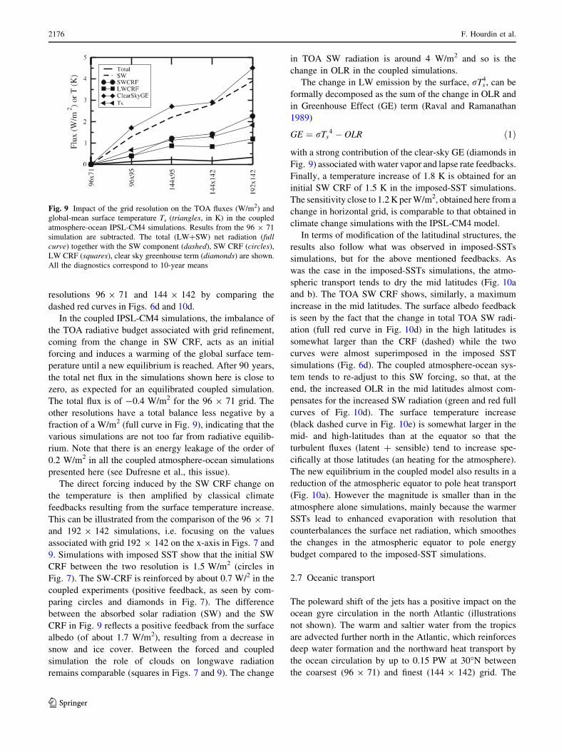
In the coupled IPSL-CM4 simulations, the imbalance of

the TOA radiative budget associated with grid refinement,

coming from the change in SW CRF, acts as an initial

forcing and induces a warming of the global surface tem-

perature until a new equilibrium is reached. After 90 years,

the total net flux in the simulations shown here is close to

zero, as expected for an equilibrated coupled simulation.

The total flux is of -0.4 W/m2 for the 96 9 71 grid. The

other resolutions have a total balance less negative by a

fraction of a W/m2 (full curve in Fig. 9), indicating that the

various simulations are not too far from radiative equilib-

rium. Note that there is an energy leakage of the order of

0.2 W/m2 in all the coupled atmosphere-ocean simulations

presented here (see Dufresne et al., this issue).

The direct forcing induced by the SW CRF change on

the temperature is then amplified by classical climate

feedbacks resulting from the surface temperature increase.

This can be illustrated from the comparison of the 96 9 71

and 192 9 142 simulations, i.e. focusing on the values

associated with grid 192 9 142 on the x-axis in Figs. 7 and

9. Simulations with imposed SST show that the initial SW

CRF between the two resolution is 1.5 W/m2 (circles in

Fig. 7). The SW-CRF is reinforced by about 0.7 W/2 in the

coupled experiments (positive feedback, as seen by com-

paring circles and diamonds in Fig. 7). The difference

between the absorbed solar radiation (SW) and the SW

CRF in Fig. 9 reflects a positive feedback from the surface

albedo (of about 1.7 W/m2), resulting from a decrease in

snow and ice cover. Between the forced and coupled

simulation the role of clouds on longwave radiation

remains comparable (squares in Figs. 7 and 9). The change

in TOA SW radiation is around 4 W/m2 and so is the

change in OLR in the coupled simulations.

The change in LW emission by the surface, rTs4, can be

formally decomposed as the sum of the change in OLR and

in Greenhouse Effect (GE) term (Raval and Ramanathan

1989)

GE ¼ rTs4 � OLR ð1Þ

with a strong contribution of the clear-sky GE (diamonds in

Fig. 9) associated with water vapor and lapse rate feedbacks.

Finally, a temperature increase of 1.8 K is obtained for an

initial SW CRF of 1.5 K in the imposed-SST simulations.

The sensitivity close to 1.2 K per W/m2, obtained here from a

change in horizontal grid, is comparable to that obtained in

climate change simulations with the IPSL-CM4 model.

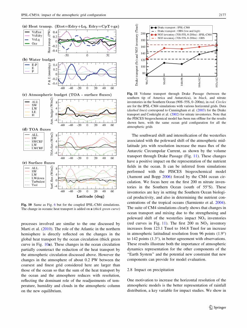
In terms of modification of the latitudinal structures, the

results also follow what was observed in imposed-SSTs

simulations, but for the above mentioned feedbacks. As

was the case in the imposed-SSTs simulations, the atmo-

spheric transport tends to dry the mid latitudes (Fig. 10a

and b). The TOA SW CRF shows, similarly, a maximum

increase in the mid latitudes. The surface albedo feedback

is seen by the fact that the change in total TOA SW radi-

ation (full red curve in Fig. 10d) in the high latitudes is

somewhat larger than the CRF (dashed) while the two

curves were almost superimposed in the imposed SST

simulations (Fig. 6d). The coupled atmosphere-ocean sys-

tem tends to re-adjust to this SW forcing, so that, at the

end, the increased OLR in the mid latitudes almost com-

pensates for the increased SW radiation (green and red full

curves of Fig. 10d). The surface temperature increase

(black dashed curve in Fig. 10e) is somewhat larger in the

mid- and high-latitudes than at the equator so that the

turbulent fluxes (latent ? sensible) tend to increase spe-

cifically at those latitudes (an heating for the atmosphere).

The new equilibrium in the coupled model also results in a

reduction of the atmospheric equator to pole heat transport

(Fig. 10a). However the magnitude is smaller than in the

atmosphere alone simulations, mainly because the warmer

SSTs lead to enhanced evaporation with resolution that

counterbalances the surface net radiation, which smoothes

the changes in the atmospheric equator to pole energy

budget compared to the imposed-SST simulations.

2.7 Oceanic transport

The poleward shift of the jets has a positive impact on the

ocean gyre circulation in the north Atlantic (illustrations

not shown). The warm and saltier water from the tropics

are advected further north in the Atlantic, which reinforces

deep water formation and the northward heat transport by

the ocean circulation by up to 0.15 PW at 30�N between

the coarsest (96 9 71) and finest (144 9 142) grid. The

Fig. 9 Impact of the grid resolution on the TOA fluxes (W/m2) and

global-mean surface temperature Ts (triangles, in K) in the coupled

atmosphere-ocean IPSL-CM4 simulations. Results from the 96 9 71

simulation are subtracted. The total (LW?SW) net radiation (fullcurve) together with the SW component (dashed), SW CRF (circles),

LW CRF (squares), clear sky greenhouse term (diamonds) are shown.

All the diagnostics correspond to 10-year means

2176 F. Hourdin et al.

123

processes involved are similar to the one discussed by

Marti et al. (2010). The role of the Atlantic in the northern

hemisphere is directly reflected on the changes in the

global heat transport by the ocean circulation (thick green

curve in Fig. 10a). These changes in the ocean circulation

partially counteract the reduction of the heat transport by

the atmospheric circulation discussed above. However the

changes in the atmosphere of about 0.2 PW between the

coarsest and finest grid considered here are larger than

those of the ocean so that the sum of the heat transport by

the ocean and the atmosphere reduces with resolution,

reflecting the dominant role of the readjustments of tem-

perature, humidity and clouds in the atmospheric column

on the new equilibrium.

The southward shift and intensification of the westerlies

associated with the poleward shift of the atmospheric mid-

latitude jets with resolution increase the mass flux of the

Antarctic Circumpolar Current, as shown by the volume

transport through Drake Passage (Fig. 11). These changes

have a positive impact on the representation of the nutrient

fields in the ocean. It can be inferred from simulations

performed with the PISCES biogeochemical model

(Aumont and Bopp 2006) forced by the CM4 ocean cir-

culation. We focus here on the first 200 m nitrate inven-

tories in the Southern Ocean (south of 55�S). These

inventories are key in setting the Southern Ocean biologi-

cal productivity, and also in determining the nutrient con-

centrations of the tropical oceans (Sarmiento et al. 2004).

The suite of CM4 simulations clearly shows that changes in

ocean transport and mixing due to the strengthening and

poleward shift of the westerlies impact NO3 inventories

(red curves in Fig. 11). The first 200 m NO3 inventory

increases from 123.1 Tmol to 164.8 Tmol for an increase

in atmospheric latitudinal resolution from 96 points (1.9�)

to 142 points (1.3�), in better agreement with observations.

These results illustrate both the importance of atmospheric

dynamics representation for the other components of the

‘‘Earth System’’ and the potential new constraint that new

components can provide for model evaluation.

2.8 Impact on precipitation

One motivation to increase the horizontal resolution of the

atmospheric models is the better representation of rainfall

distribution, a key variable for impact studies. We show in

(a)

(b)

(c)

(d)

(e)

Fig. 10 Same as Fig. 6 but for the coupled IPSL-CM4 simulations.

The change in oceanic heat transport is added on a (thick green curve)

Fig. 11 Volume transport through Drake Passage (between the

southern tip of America and Antarctica), in black, and nitrate

inventories in the Southern Ocean (90S–55S, 0–200m), in red. Circlesare for the IPSL-CM4 simulations with various horizontal grids. Data

(dashed lines) correspond to Cunningham et al. (2003) for the Drake

transport and Conkright et al. (2002) for nitrate inventories. Note that

the PISCES biogeochemical model has been run offline for the results

shown here, with the same ocean grid configuration for all the

atmospheric grids

IPSL-CM5A: impact of the atmospheric grid configuration 2177

123

GPCP climatology

LMDZ4 – 96 × 71

LMDZ4 – 280 × 192

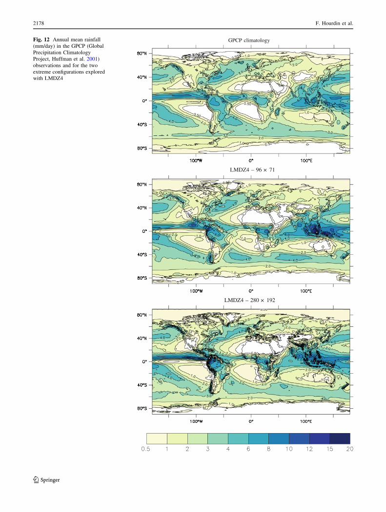
Fig. 12 Annual mean rainfall

(mm/day) in the GPCP (Global

Precipitation Climatology

Project, Huffman et al. 2001)

observations and for the two

extreme configurations explored

with LMDZ4

2178 F. Hourdin et al.

123

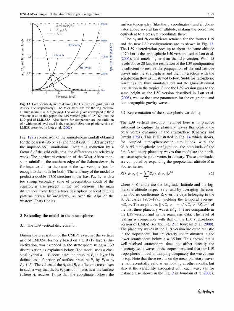
Fig. 12a a comparison of the annual-mean rainfall obtained

for the coarsest (96 9 71) and finest (280 9 192) grids for

the imposed-SST simulations. Despite a reduction by a

factor 8 of the grid cells area, the differences are relatively

weak. The northward extension of the West Africa mon-

soon rainfall at the southern edge of the Sahara desert, is

for instance almost the same in the two versions (not far

enough to the north for both). The tendency of the model to

predict a double ITCZ structure in the East Pacific, with a

too strong secondary zone of precipitation south of the

equator, is also present in the two versions. The main

differences come from a finer description of local rainfall

patterns driven by orography, as over the Alps or the

western Ghats (India).

3 Extending the model to the stratosphere

3.1 The L39 vertical discretization

During the preparation of the CMIP5 exercise, the vertical

grid of LMDZ4, formerly based on a L19 (19 layers) dis-

cretization, was extended in the stratosphere using a L39

discretization as explained below. The model uses a clas-

sical hybrid r - P coordinate: the pressure Pl in layer l is

defined as a function of surface pressure Ps by Pl = Al

Ps ? Bl. The values of the Al and Bl coefficients are chosen

in such a way that the Al Ps part dominates near the surface

(where Al reaches 1), so that the coordinate follows the

surface topography (like the r coordinates), and Bl domi-

nates above several km of altitude, making the coordinate

equivalent to a pressure coordinate there.

The Al and Bl coefficients retained for the former L19

and the new L39 configurations are as shown in Fig. 13.

The L39 discretization goes up to about the same altitude

of 70 km as the stratospheric L50 version used in Lott et al.

(2005), and much higher than the L19 version. With 15

levels above 20 km, the resolution of the L39 configuration

is sufficient to resolve the propagation of the mid-latitude

waves into the stratosphere and their interaction with the

zonal-mean flow as illustrated below. Sudden-stratospheric

warmings are thus simulated, but not the Quasi-Biennial

Oscillation in the tropics. Since the L39 version goes to the

same height as the L50 version described in Lott et al.

(2005), we use the same parameters for the orographic and

non-orographic gravity waves.

3.2 Representation of the stratospheric variability

The L39 vertical resolution retained here is in practice

sufficient to capture the planetary waves that control the

polar vortex dynamics in the stratosphere (Charney and

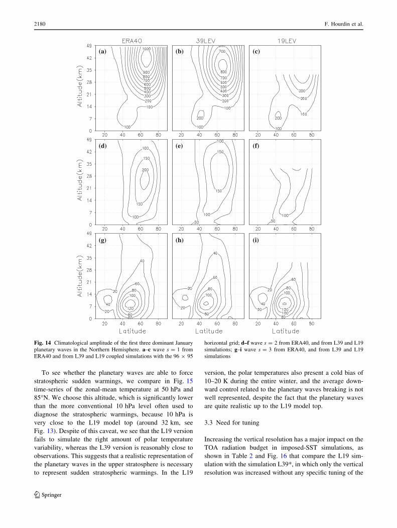
Drazin 1961). This is illustrated in Fig. 14 which shows,

for coupled atmosphere-ocean simulations with the

96 9 95 atmospheric configuration, the amplitude of the

first 3 stationary planetary waves that modulate the north-

ern stratospheric polar vortex in January. These amplitudes

are computed by expanding the geopotential altitude Z in

Fourier series,

Zðk;/; z; tÞ ¼X

s

Zsðs;/; z; tÞeisk ð2Þ

where k, /, and z are the longitude, latitude and the log-

pressure altitude respectively, and by averaging the com-

plex Fourier coefficients Zs over the days belonging to the

30 Januaries 1976–1995, yielding the temporal average

\Zs [. The amplitudes k\Zs [ k ¼ffiffiffiffiffiffiffiffiffiffiffiffiffiffiffiffiffiffiffiffiffiffiffiffiffiffiffiffiffiffiffiffi\Zs [ \Zs [ �p

of

the first three planetary waves (Fig. 14) are comparable in

the L39 version and in the reanalysis data. The level of

realism is comparable with that of the L50 stratospheric

version of LMDZ (see the Fig. 2 in Jourdain et al. 2008).

The planetary waves in the L19 version are quite realistic

in the troposphere, but are clearly underestimated in the

lower stratosphere below z = 35 km. This shows that a

well-resolved stratosphere does not affect directly the

planetary-scale waves in the troposphere, and that our L19

tropospheric model is damping adequately the waves near

its top. Note that these results on the mean planetary waves

remain essentially valid when looking at other months but

also at the variability associated with each wave (as for

instance also shown in the Fig. 2 in Jourdain et al. 2008).

Fig. 13 Coefficients Al and Bl defining the L39 vertical grid (dot and

dashes line respectively). The thick lines are for the log pressure

altitude in km: z = 7. log(Ps/Pl). The values given correspond to the 2

versions used in this paper: the L19 vertical grid of LMDZ4 and the

L39 grid of LMDZ5A. Also shown for comparison are the variation

of z with model level used in the standard L50 stratospheric version of

LMDZ presented in Lott et al. (2005)

IPSL-CM5A: impact of the atmospheric grid configuration 2179

123

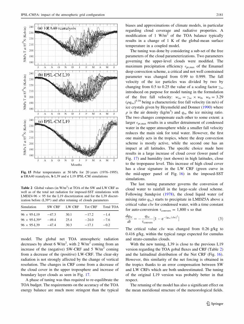
To see whether the planetary waves are able to force

stratospheric sudden warmings, we compare in Fig. 15

time-series of the zonal-mean temperature at 50 hPa and

85�N. We choose this altitude, which is significantly lower

than the more conventional 10 hPa level often used to

diagnose the stratospheric warmings, because 10 hPa is

very close to the L19 model top (around 32 km, see

Fig. 13). Despite of this caveat, we see that the L19 version

fails to simulate the right amount of polar temperature

variability, whereas the L39 version is reasonably close to

observations. This suggests that a realistic representation of

the planetary waves in the upper stratosphere is necessary

to represent sudden stratospheric warmings. In the L19

version, the polar temperatures also present a cold bias of

10–20 K during the entire winter, and the average down-

ward control related to the planetary waves breaking is not

well represented, despite the fact that the planetary waves

are quite realistic up to the L19 model top.

3.3 Need for tuning

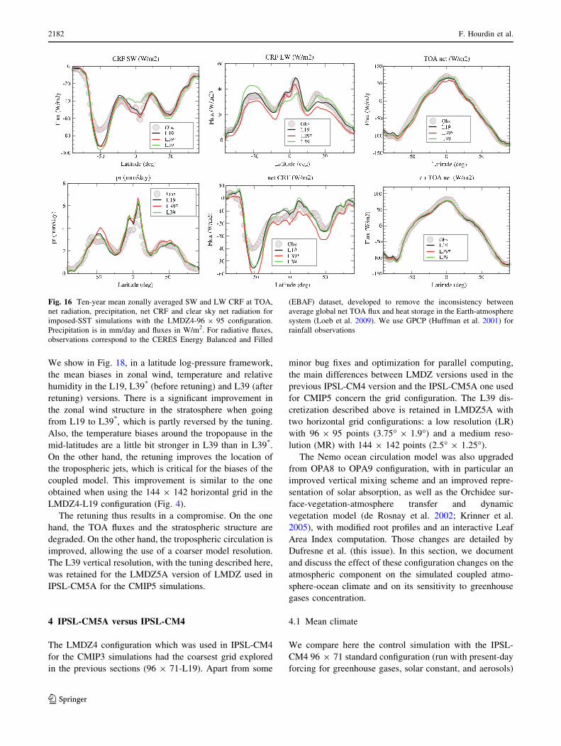
Increasing the vertical resolution has a major impact on the

TOA radiation budget in imposed-SST simulations, as

shown in Table 2 and Fig. 16 that compare the L19 sim-

ulation with the simulation L39*, in which only the vertical

resolution was increased without any specific tuning of the

(a) (b) (c)

(d) (e) (f)

(g) (h) (i)

Fig. 14 Climatological amplitude of the first three dominant January

planetary waves in the Northern Hemisphere. a–c wave s = 1 from

ERA40 and from L39 and L19 coupled simulations with the 96 9 95

horizontal grid; d–f wave s = 2 from ERA40, and from L39 and L19

simulations; g–i wave s = 3 from ERA40, and from L39 and L19

simulations

2180 F. Hourdin et al.

123

model. The global net TOA atmospheric radiation

decreases by about 6 W/m2, with 2 W/m2 coming from an

increase of the (negative) SW-CRF and 5 W/m2 coming

from a decrease of the (positive) LW-CRF. The clear-sky

radiation is not strongly affected by the change of vertical

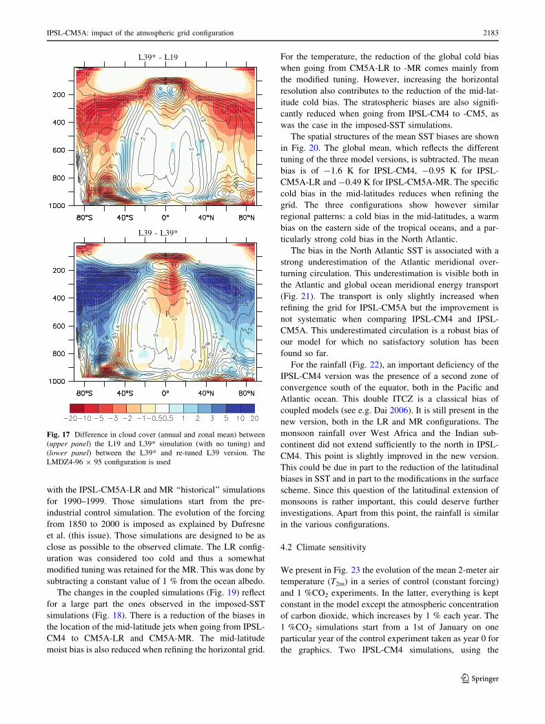
resolution. The changes in CRF come from a decrease of

the cloud cover in the upper troposphere and increase of

boundary layer clouds as seen in Fig. 17.

A phase of tuning was thus required to re-equilibrate the

TOA budget. The requirements on the accuracy of the TOA

energy balance are much more stringent than the typical

biases and approximations of climate models, in particular

regarding cloud coverage and radiative properties. A

modification of 1 W/m2 of the TOA balance typically

results in a change of 1 K of the global-mean surface

temperature in a coupled model.

The tuning was done by considering a sub-set of the free

parameters of the cloud parameterizations. Two parameters

governing the upper-level clouds were modified. The

maximum precipitation efficiency �pr;max of the Emanuel

deep convection scheme, a critical and not well constrained

parameter was changed from 0.99 to 0.999. The fall

velocity of the ice particles was divided by two by

changing from 0.5 to 0.25 the value of a scaling factor ciw

introduced on purpose for model tuning in the formulation

of the free fall velocity: wiw = ciw 9 w0, w0 = 3.29

(qqiw)0.16 being a characteristic free fall velocity (in m/s) of

ice crystals given by Heymsfield and Donner (1990) where

q is the air density (kg/m3) and qiw the ice mixing ratio.

The two changes compensate each other to some extent: a

larger �pr;max results in a smaller detrainment of condensed

water in the upper atmosphere while a smaller fall velocity

reduces the main sink for total water. However, the first

one mainly acts in the tropics, where the deep convection

scheme is mostly active, while the second one has an

impact at all latitudes. The specific choice made here

results in a large increase of cloud cover (lower panel of

Fig. 17) and humidity (not shown) in high latitudes, close

to the tropopause level. This increase of high cloud cover

has a clear signature in the LW CRF (green curve in

the mid-upper panel of Fig. 16) in the imposed-SST

simulations.

The last tuning parameter governs the conversion of

cloud water to rainfall in the large-scale cloud scheme.

Following Sundqvist (1978), the cloud liquid water (of

mixing ratio qlw) starts to precipitate in LMDZ5A above a

critical value clw for condensed water, with a time constant

for auto-conversion sconvers = 1,800 s so that

dqlw

dt¼ � qlw

sconvers

½1� e�ðqlw=clwÞ2 � ð3Þ

The critical value clw was changed from 0.26 g/kg to

0.416 g/kg, within the typical range expected for cumulus

and strato-cumulus clouds.

With the new tuning, L39 is close to the previous L19

version regarding the TOA gobal fluxes and CRF (Table 2)

and the latitudinal distribution of the Net CRF (Fig. 16).

However, this similarity of the net forcing is obtained in

the tropics thanks to an error compensation between SW

and LW CRFs which are both underestimated. The tuning

of the original L19 version was probably better in that

respect.

The retuning of the model has also a significant effect on

the mean meridional structure of the meteorological fields.

(a)

(b)

(c)

Fig. 15 Polar temperatures at 50 hPa for 20 years (1976–1995).

a ERA40 reanalysis, b L39 and c L19 IPSL-CM simulations

Table 2 Global values (in W/m2) at TOA of the SW and LW CRF as

well as of the total net radiation for imposed-SST simulations with

LMDZ4-96 9 95 for the L19 discretization and for the L39 discret-

ization before (L39*) and after retuning of clouds parameters

Simulation SW CRF LW CRF Tot CRF Total TOA

96 9 95-L19 -47.3 30.1 -17.2 -1.4

96 9 95-L39* -49.4 25.4 -24.0 -7.6

96 9 95-L39 -47.4 30.3 -17.1 -0.2

IPSL-CM5A: impact of the atmospheric grid configuration 2181

123

We show in Fig. 18, in a latitude log-pressure framework,

the mean biases in zonal wind, temperature and relative

humidity in the L19, L39* (before retuning) and L39 (after

retuning) versions. There is a significant improvement in

the zonal wind structure in the stratosphere when going

from L19 to L39*, which is partly reversed by the tuning.

Also, the temperature biases around the tropopause in the

mid-latitudes are a little bit stronger in L39 than in L39*.

On the other hand, the retuning improves the location of

the tropospheric jets, which is critical for the biases of the

coupled model. This improvement is similar to the one

obtained when using the 144 9 142 horizontal grid in the

LMDZ4-L19 configuration (Fig. 4).

The retuning thus results in a compromise. On the one

hand, the TOA fluxes and the stratospheric structure are

degraded. On the other hand, the tropospheric circulation is

improved, allowing the use of a coarser model resolution.

The L39 vertical resolution, with the tuning described here,

was retained for the LMDZ5A version of LMDZ used in

IPSL-CM5A for the CMIP5 simulations.

4 IPSL-CM5A versus IPSL-CM4

The LMDZ4 configuration which was used in IPSL-CM4

for the CMIP3 simulations had the coarsest grid explored

in the previous sections (96 9 71-L19). Apart from some

minor bug fixes and optimization for parallel computing,

the main differences between LMDZ versions used in the

previous IPSL-CM4 version and the IPSL-CM5A one used

for CMIP5 concern the grid configuration. The L39 dis-

cretization described above is retained in LMDZ5A with

two horizontal grid configurations: a low resolution (LR)

with 96 9 95 points (3.75� 9 1.9�) and a medium reso-

lution (MR) with 144 9 142 points (2.5� 9 1.25�).

The Nemo ocean circulation model was also upgraded

from OPA8 to OPA9 configuration, with in particular an

improved vertical mixing scheme and an improved repre-

sentation of solar absorption, as well as the Orchidee sur-

face-vegetation-atmosphere transfer and dynamic

vegetation model (de Rosnay et al. 2002; Krinner et al.

2005), with modified root profiles and an interactive Leaf

Area Index computation. Those changes are detailed by

Dufresne et al. (this issue). In this section, we document

and discuss the effect of these configuration changes on the

atmospheric component on the simulated coupled atmo-

sphere-ocean climate and on its sensitivity to greenhouse

gases concentration.

4.1 Mean climate

We compare here the control simulation with the IPSL-

CM4 96 9 71 standard configuration (run with present-day

forcing for greenhouse gases, solar constant, and aerosols)

Fig. 16 Ten-year mean zonally averaged SW and LW CRF at TOA,

net radiation, precipitation, net CRF and clear sky net radiation for

imposed-SST simulations with the LMDZ4-96 9 95 configuration.

Precipitation is in mm/day and fluxes in W/m2. For radiative fluxes,

observations correspond to the CERES Energy Balanced and Filled

(EBAF) dataset, developed to remove the inconsistency between

average global net TOA flux and heat storage in the Earth-atmosphere

system (Loeb et al. 2009). We use GPCP (Huffman et al. 2001) for

rainfall observations

2182 F. Hourdin et al.

123

with the IPSL-CM5A-LR and MR ‘‘historical’’ simulations

for 1990–1999. Those simulations start from the pre-

industrial control simulation. The evolution of the forcing

from 1850 to 2000 is imposed as explained by Dufresne

et al. (this issue). Those simulations are designed to be as

close as possible to the observed climate. The LR config-

uration was considered too cold and thus a somewhat

modified tuning was retained for the MR. This was done by

subtracting a constant value of 1 % from the ocean albedo.

The changes in the coupled simulations (Fig. 19) reflect

for a large part the ones observed in the imposed-SST

simulations (Fig. 18). There is a reduction of the biases in

the location of the mid-latitude jets when going from IPSL-

CM4 to CM5A-LR and CM5A-MR. The mid-latitude

moist bias is also reduced when refining the horizontal grid.

For the temperature, the reduction of the global cold bias

when going from CM5A-LR to -MR comes mainly from

the modified tuning. However, increasing the horizontal

resolution also contributes to the reduction of the mid-lat-

itude cold bias. The stratospheric biases are also signifi-

cantly reduced when going from IPSL-CM4 to -CM5, as

was the case in the imposed-SST simulations.

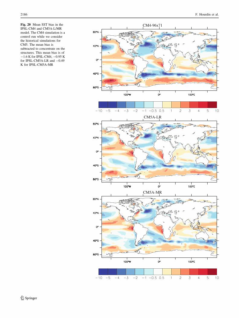
The spatial structures of the mean SST biases are shown

in Fig. 20. The global mean, which reflects the different

tuning of the three model versions, is subtracted. The mean

bias is of -1.6 K for IPSL-CM4, -0.95 K for IPSL-

CM5A-LR and -0.49 K for IPSL-CM5A-MR. The specific

cold bias in the mid-latitudes reduces when refining the

grid. The three configurations show however similar

regional patterns: a cold bias in the mid-latitudes, a warm

bias on the eastern side of the tropical oceans, and a par-

ticularly strong cold bias in the North Atlantic.

The bias in the North Atlantic SST is associated with a

strong underestimation of the Atlantic meridional over-

turning circulation. This underestimation is visible both in

the Atlantic and global ocean meridional energy transport

(Fig. 21). The transport is only slightly increased when

refining the grid for IPSL-CM5A but the improvement is

not systematic when comparing IPSL-CM4 and IPSL-

CM5A. This underestimated circulation is a robust bias of

our model for which no satisfactory solution has been

found so far.

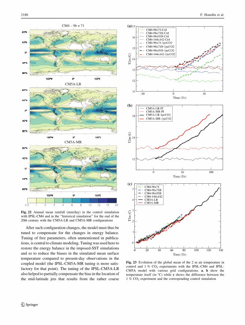
For the rainfall (Fig. 22), an important deficiency of the

IPSL-CM4 version was the presence of a second zone of

convergence south of the equator, both in the Pacific and

Atlantic ocean. This double ITCZ is a classical bias of

coupled models (see e.g. Dai 2006). It is still present in the

new version, both in the LR and MR configurations. The

monsoon rainfall over West Africa and the Indian sub-

continent did not extend sufficiently to the north in IPSL-

CM4. This point is slightly improved in the new version.

This could be due in part to the reduction of the latitudinal

biases in SST and in part to the modifications in the surface

scheme. Since this question of the latitudinal extension of

monsoons is rather important, this could deserve further

investigations. Apart from this point, the rainfall is similar

in the various configurations.

4.2 Climate sensitivity

We present in Fig. 23 the evolution of the mean 2-meter air

temperature (T2m) in a series of control (constant forcing)

and 1 %CO2 experiments. In the latter, everything is kept

constant in the model except the atmospheric concentration

of carbon dioxide, which increases by 1 % each year. The

1 %CO2 simulations start from a 1st of January on one

particular year of the control experiment taken as year 0 for

the graphics. Two IPSL-CM4 simulations, using the

L39* - L19

L39 - L39*

Fig. 17 Difference in cloud cover (annual and zonal mean) between

(upper panel) the L19 and L39* simulation (with no tuning) and

(lower panel) between the L39* and re-tuned L39 version. The

LMDZ4-96 9 95 configuration is used

IPSL-CM5A: impact of the atmospheric grid configuration 2183

123

coarsest horizontal grids (96 9 71 and 96 9 95), were

tuned by lowering the surface albedo (by subtracting 1 and

0.9 % respectively), so as to obtain an averaged global

mean temperature close to that of the 144 9 142 configu-

ration for the control simulations run with present-day

greenhouse gases concentrations. Those simulations are

called 96 9 71B and 96 9 95B. The 96 9 71B simulation

is still 0.5 K colder than 96 9 95B and 144 9 142

(Fig. 23a). Control simulations and climate sensitivity

experiments were done with both 96 9 71 and 96 9 71B

to check whether the tuning affects the climate sensitivity.

For the IPSL-CM5A model, the tuned (lowered) ocean

albedo also explains a large part of the difference between

the LR and MR configurations (Fig. 23b).

Despite those changes in grid configuration, in tuning or

in the mean temperature biases, the transient climate

response (defined as the difference between the 1 %CO2

and control experiments at time of CO2 doubling, i.e.

around year 70) is almost the same for all the model con-

figurations as illustrated in the lower panel of Fig. 23. The

ocean uptake is also comparable for all the simulations (not

shown). A rigorous climate sensitivity analysis based on

both 1 % CO2 and abrupt 4 9 CO2 experiments shows that

the climate sensitivity and feedback parameters differ by

less than 10 % between the IPSL-CM4, IPSL-CM5A-LR

and -MR models (see Dufresne et al., this issue).

The regional distribution of global warming (left part of

Fig. 24 for IPSL-CM4 and of Fig. 25 for -CM5A) also

shows quite consistent results between the different ver-

sions, and reflects the usual robust aspects of climate

change simulations: a stronger warming over the continents

(where evaporative cooling is limited) than over oceans, a

stronger warming in the (more continental) northern

hemisphere than in the southern one, and in high than in

low latitudes in the northern hemisphere. The simulations

also show, in a rather consistent way, a weak warming in

the Southern Ocean and in the North Atlantic.

The situation is a bit different for changes in the mean

rainfall. Some aspects appear to be quite robust, such as the

global increase of rainfall in the ITCZ/SPCZ region, and a

(TU (m/s) ° RH (%))C99

×99

- L

19

Pseu

do a

ltitu

de (

km)

99×

99 -

L39

*

Pseu

do a

ltitu

de (

km)

99×

99 -

L39

Pseu

do a

ltitu

de (

km)

Fig. 18 Mean meridional structure of the Zonal wind (m/s, left), temperature (�C, middle) and relative humidity for the L19, L39* and L39

forced simulations with the LR horizontal grid. The vertical axis is a pseudo-altitude (-H ln(p/ps), with H = 7 km)

2184 F. Hourdin et al.

123

relative drying at around 30–40 degrees latitude in both

hemispheres, also a rather robust feature of CMIP3 pro-

jections (Held and Soden 2006). However, when looking at

regional changes over the continents, results differ quite

significantly between IPSL-CM4 and CM5A. Generally

speaking, the CM4 configuration tends to predict a stronger

drying (in particular over Amazonia, central Africa, India)

than CM5A does, while, for each model, the results are

much more consistent when varying the horizontal reso-

lution. The differences between the CM4 and CM5A

results are probably due to some significant changes in the

Orchidee land-surface model between the two versions: a

bug fix which had a particularly strong impact in semi-arid

regions, a soil reservoir twice as deep in CM5A and the

activation of the CO2 cycle which influences the Leaf Area

Index (Dufresne et al., this issue). Whether one of those

changes is responsible for the changes observed is a

question which could deserve further investigations.

5 Conclusions

We have explored the impact of the horizontal and vertical

grid configuration of an atmospheric general circulation

model on the results of both imposed-SST and coupled

simulations, focusing on the representation of the mean

climate and on the climate sensitivity to greenhouse gases

concentration.

The refinement of the horizontal grid has a significant

and systematic impact on the model biases, in particular on

the latitude of the jets and on the humidity and temperature

in the mid latitudes. Refining the grid in latitude rather

than in longitude has a stronger impact on the latitude of

the mid-latitude jets in the dynamical core experiments

(Guemas and Codron 2011) and in the imposed-SST cli-

mate simulations, and a stronger impact on the reduction of

the cold mid-latitude SST bias with respect to Equator in

the coupled experiments.

(TU (m/s) ° RH (%))CIP

SL-C

M4

Pres

sure

(hP

a)

IPSL

-CM

5A-L

R

Pres

sure

(hP

a)

IPSL

-CM

5A-M

R

Pres

sure

(hP

a)

Fig. 19 Mean meridional structure of the Zonal wind (m/s, left),temperature (oC, middle) and relative humidity (%) for the IPSL-

CM4, IPSL-CM5A-LR and -MR simulations. The IPSL-CM4

simulation corresponds to a control run in present conditions while

we show for IPSL-CM5A-LR and -MR the 1990–1999 decade of

historical runs

IPSL-CM5A: impact of the atmospheric grid configuration 2185

123

CM4-96x71

CM5A-LR

CM5A-MR

Fig. 20 Mean SST bias in the

IPSL-CM4 and CM5A-L/MR

model. The CM4 simulation is a

control run while we consider

the historical simulations for

CM5. The mean bias is

subtracted to concentrate on the

structures. This mean bias is of

-1.6 K for IPSL-CM4, -0.95 K

for IPSL-CM5A-LR and -0.49

K for IPSL-CM5A-MR

2186 F. Hourdin et al.

123

The changes of atmospheric dynamics when refining the

grid are associated with significant changes in the meridi-

onal transport of heat and moisture. In mid-latitudes, grid

refinement (in particular in latitude) reduces systematically

a strong moist bias of the coarsest configurations, which

results in less low-level clouds. In imposed-SST simula-

tions, this decrease in cloudiness weakens the vertically

integrated tropospheric radiative cooling and thus reduces

the cold atmospheric bias in mid-latitudes. In coupled

atmosphere-ocean simulations, the reduced cloud cover

enhances the short-wave radiation at the surface in mid

latitudes, and thus contributes to reduce the cold SST bias

in that region. Changes in the tropical circulation are also

observed when increasing the resolution in longitude that

also contribute to reduce the low-level cloud cover.

Starting the explanation from the change of dynamics is

somewhat arbitrary since it is possible that the changes of

atmospheric transport at work in the full climate model are

influenced by other processes, coming for instance from a

direct sensitivity of the physical parameterizations to the

grid size. However, the fact that the jet displacement

mimics that observed in the idealized simulations with

newtonian cooling, and that we are able to derive a

complete and consistent explanation of the changes

observed apart from this initial change, suggests that it

could explain at least a large part of the modifications

observed. This point would deserve however additional

investigations, including for instance the use of idealized

water-like tracers in idealized simulations with newtonian

cooling.

It is shown also that the extension of the vertical grid to

higher levels improves the representation of the strato-

spheric mean flow and of stratospheric sudden warmings.

Changing the grid configuration also has an impact on the

global energy balance. Refinement of the horizontal grid

results in a warmer climate in the IPSL-CM model as a

consequence of the above mentioned decrease in low-level

cloud cover which induces weaker (less negative) SW-CRF.

The impact of refining the vertical grid is even stronger and is

mainly related to changes in high-level cloudiness. The

modifications are as large as 3 W/m2 when refining the

horizontal grid from 96 9 71 to 280 9 192, or about -6

W/m2 when changing the vertical discretization from L19 to

L39. In the coupled model, the model global radiation bal-

ance is restored through an increase of the global-mean near-

surface temperature, by about 1.2 K per W/m2.

Fig. 21 Global (top) and

Atlantic (bottom) total

meridional energy transport by

the ocean (in PW) in the IPSL-

CM4, IPSL-CM5A-LR and

IPSL-CM5A-MR simulations.

Heat transport estimates

(Ganachaud and Wunsch 2003)

are obtained by inversion or

hydrographic data from the

World ocean circulation

experiment

IPSL-CM5A: impact of the atmospheric grid configuration 2187

123

After such configuration changes, the model must thus be

tuned to compensate for the changes in energy balance.

Tuning of free parameters, often unmentioned in publica-

tions, is central to climate modeling. Tuning was used here to

restore the energy balance in the imposed-SST simulations

and so to reduce the biases in the simulated mean surface

temperature compared to present-day observations in the

coupled model (the IPSL-CM5A-MR tuning is more satis-

factory for that point). The tuning of the IPSL-CM5A-LR

also helped to partially compensate the bias in the location of

the mid-latitude jets that results from the rather coarse

CM4 – 96 × 71

CM5A-LR

CM5A-MR

Fig. 22 Annual mean rainfall (mm/day) in the control simulation

with IPSL-CM4 and in the ‘‘historical simulation’’ for the end of the

20th century with the CM5A-LR and CM5A-MR configurations

(a)

(b)

(c)

Fig. 23 Evolution of the global mean of the 2 m air temperature in

control and 1 % CO2 experiments with the IPSL-CM4 and IPSL-

CM5A model with various grid configurations. a, b show the

temperature itself (in �C) while c shows the difference between the

1 % CO2 experiment and the corresponding control simulation

2188 F. Hourdin et al.

123

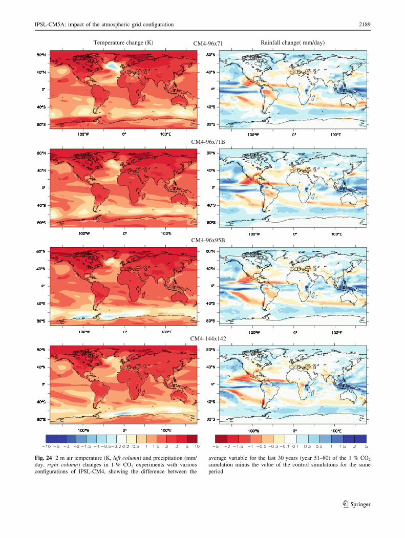
Rainfall change( mm/day)Temperature change (K) CM4-96x71

CM4-96x71B

CM4-96x95B

CM4-144x142

Fig. 24 2 m air temperature (K, left column) and precipitation (mm/

day, right column) changes in 1 % CO2 experiments with various

configurations of IPSL-CM4, showing the difference between the

average variable for the last 30 years (year 51–80) of the 1 % CO2

simulation minus the value of the control simulations for the same

period

IPSL-CM5A: impact of the atmospheric grid configuration 2189

123

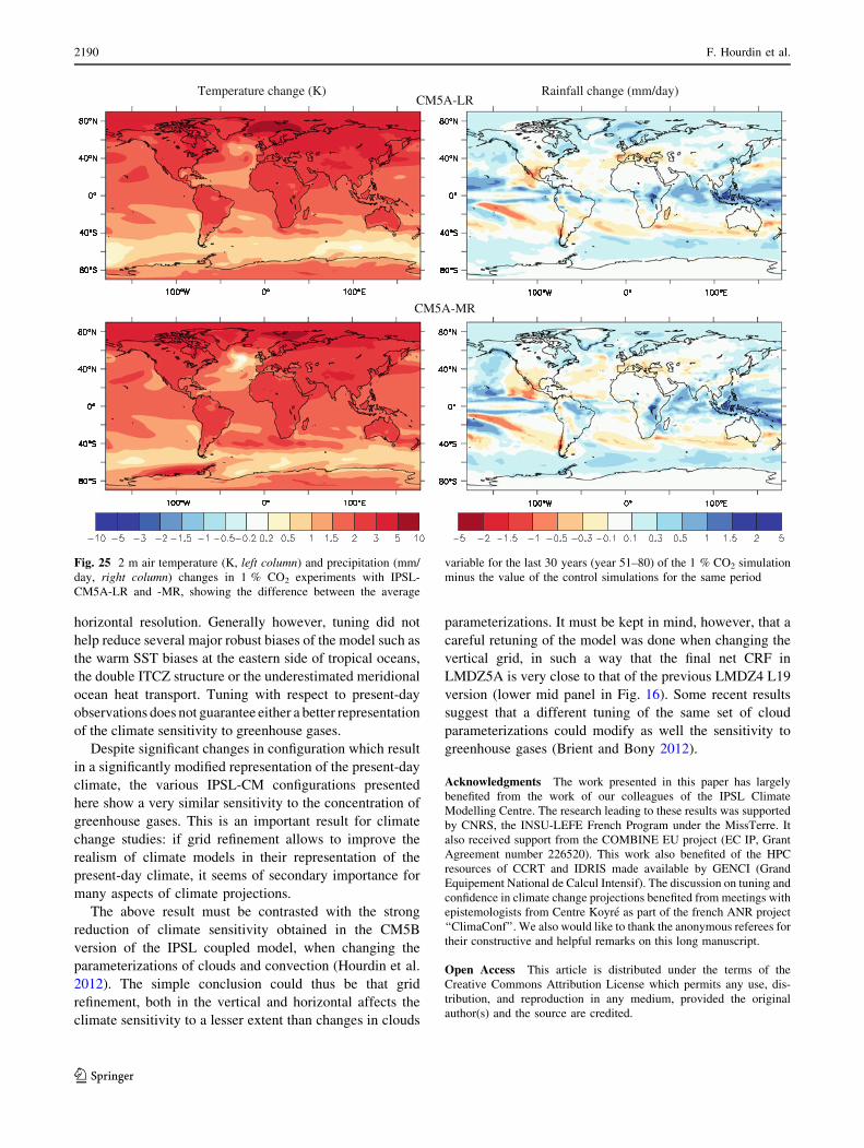
horizontal resolution. Generally however, tuning did not

help reduce several major robust biases of the model such as

the warm SST biases at the eastern side of tropical oceans,

the double ITCZ structure or the underestimated meridional

ocean heat transport. Tuning with respect to present-day

observations does not guarantee either a better representation

of the climate sensitivity to greenhouse gases.

Despite significant changes in configuration which result

in a significantly modified representation of the present-day

climate, the various IPSL-CM configurations presented

here show a very similar sensitivity to the concentration of

greenhouse gases. This is an important result for climate

change studies: if grid refinement allows to improve the

realism of climate models in their representation of the

present-day climate, it seems of secondary importance for

many aspects of climate projections.

The above result must be contrasted with the strong

reduction of climate sensitivity obtained in the CM5B

version of the IPSL coupled model, when changing the

parameterizations of clouds and convection (Hourdin et al.

2012). The simple conclusion could thus be that grid

refinement, both in the vertical and horizontal affects the

climate sensitivity to a lesser extent than changes in clouds

parameterizations. It must be kept in mind, however, that a

careful retuning of the model was done when changing the

vertical grid, in such a way that the final net CRF in

LMDZ5A is very close to that of the previous LMDZ4 L19

version (lower mid panel in Fig. 16). Some recent results

suggest that a different tuning of the same set of cloud

parameterizations could modify as well the sensitivity to

greenhouse gases (Brient and Bony 2012).

Acknowledgments The work presented in this paper has largely

benefited from the work of our colleagues of the IPSL Climate

Modelling Centre. The research leading to these results was supported

by CNRS, the INSU-LEFE French Program under the MissTerre. It

also received support from the COMBINE EU project (EC IP, Grant

Agreement number 226520). This work also benefited of the HPC

resources of CCRT and IDRIS made available by GENCI (Grand

Equipement National de Calcul Intensif). The discussion on tuning and

confidence in climate change projections benefited from meetings with

epistemologists from Centre Koyre as part of the french ANR project

‘‘ClimaConf’’. We also would like to thank the anonymous referees for

their constructive and helpful remarks on this long manuscript.

Open Access This article is distributed under the terms of the

Creative Commons Attribution License which permits any use, dis-

tribution, and reproduction in any medium, provided the original

author(s) and the source are credited.

Rainfall change (mm/day)Temperature change (K)CM5A-LR

CM5A-MR

Fig. 25 2 m air temperature (K, left column) and precipitation (mm/

day, right column) changes in 1 % CO2 experiments with IPSL-

CM5A-LR and -MR, showing the difference between the average

variable for the last 30 years (year 51–80) of the 1 % CO2 simulation

minus the value of the control simulations for the same period

2190 F. Hourdin et al.

123

References

Aumont O, Bopp L (2006) Globalizing results from ocean in situ iron

fertilization studies. Global Biogeochem Cycles 20:GB2017.

doi:10.1029/2005GB002591

Baldwin MP, Dunkerton TJ (1999) Propagation of the Arctic

oscillation from the stratosphere to the troposphere. J Geophys

Res 1043:30,937–30,946. doi:10.1029/1999JD900445

Baldwin MP, Gray LJ, Dunkerton TJ, Hamilton K, Haynes PH,

Randel WJ, Holton JR, Alexander MJ, Hirota I, Horinouchi T,

Jones DBA, Kinnersley JS, Marquardt C, Sato K, Takahashi M

(2001) The quasi-biennial oscillation. Rev Geophys 39:179–230.

doi:10.1029/1999RG000073

Bony S, Emanuel KA (2001) A parameterization of the cloudiness

associated with cumulus convection; evaluation using TOGA

COARE data. J Atmos Sci 58:3158–3183

Bony S, Dufresne JL, Le Treut H, Morcrette JJ, Senior C (2004) On

dynamic and thermodynamic components of cloud changes.

Clim Dyn 22:71–86. doi:10.1007/s00382-003-0369-6

Braconnot P, Hourdin F, Bony S, Dufresne JL, Grandpeix JY, Marti O

(2007) Impact of different convective cloud schemes on the

simulation of the tropical seasonal cycle in a coupled ocean-

atmosphere model. Clim Dyn 29:501–520

Brient F, Bony S (2012) Interpretation of the positive low-cloud

feedback predicted by a climate model under global warming.

Clim Dyn 6. doi:10.1007/s00382-011-1279-7

Byrkjedal O, Esau I, Kvamsto NG (2008) Sensitivity of simulated

wintertime Arctic atmosphere to vertical resolution in the

arpege/ifs model. Clim Dyn 30(7–8):687

Charney JG, Drazin PG (1961) Propagation of planetary-scale

disturbances from the lower into the upper atmosphere. J Geo-

phys Res 66:83–109. doi:10.1029/JZ066i001p00083

Conkright ME, Locarnini R, Garcia H, O’Brien T, Boyer T, Stephens C,

Antonov J (2002) World ocean atlas 2001: objective analyses, data

statistics and figures cd-romdocumentation. National Oceanographic

Data Center Internal Report 17, US Department of Commerce

Cunningham SA, Alderson SG, King BA, Brandon MA (2003)

Transport and variability of the Antarctic circumpolar current in

drake passage. J Geophys Res (Oceans) 108:8084. doi:10.1029/

2001JC001147

Dai A (2006) Precipitation characteristics in eighteen coupled climate

models. J Clim 19:4605–4630B. doi:10.1175/JCLI3884.1

de Rosnay P, Polcher J, Bruen M, Laval K (2002) Impact of a

physically based soil water flow and soil-plant interaction

representation for modeling large scale land surface processes.

J Geophys Res 107. doi:10.1029/2001JD000634

Deardorff JW (1966) The counter-gradient heat-flux in the lower

atmosphere and in the laboratory. J Atmos Sci 23:503–506

Deque M, Dreverton C, Braun A, Cariolle D (1994) The Arpege/IFS

atmosphere model: a contribution to the french community

climate modelling. Clim Dyn 10:249–266

Emanuel KA (1991) A scheme for representing cumulus convection

in large-scale models. J Atmos Sci 48:2313–2335

Ganachaud A, Wunsch C (2003) Large-scale ocean heat and

freshwater transports during the world ocean circulation exper-

iment. J Clim 16:696–705. doi:10.1175/1520-0442(2003)016

\0696:LSOHAF[2.0.CO;2

Guemas V, Codron F (2011) Differing impacts of resolution changes

in latitude and longitude on the mid-latitudes in the LMDZ

GCM. J Clim. doi:10.1175/2011JCLI4093.1

Hack JJ, Caron JM, Danabasoglu G, Oleson KW, Bitz C, Truesdale

JE (2006) Ccsm-cam3 climate simulation sensitivity to changes

in horizontal resolution. J Clim 19:2267–2289

Held IM, Soden BJ (2006) Robust responses of the hydrological cycle to

global warming. J Clim 19:5686–5699. doi:10.1175/JCLI3990.1

Held IM, Suarez MJ (1994) A proposal of the dynamical cores of

atmospehric general circulation models. Bull Am Meteor Soc

75(10):1825–1830

Heymsfield AJ, Donner LJ (1990) A scheme for parameterizing ice-

cloud water content in general circulation models. J Atmos Sci

47:1865–1877. doi:10.1175/1520-0469(1990)047\1865:ASFPIC[2.0.CO;2

Hourdin F, Musat I, Bony S, Braconnot P, Codron F, Dufresne JL,

Fairhead L, Filiberti MA, Friedlingstein P, Grandpeix JY,

Krinner G, Levan P, Li ZX, Lott F (2006) The LMDZ4 general

circulation model: climate performance and sensitivity to

parametrized physics with emphasis on tropical convection.

Clim Dyn 27:787–813. doi:10.1007/s00382-006-0158-0

Hourdin F, Grandpeix JY, Rio C, Bony S, Jam A, Cheruy F, Rochetin N,

Fairhead L, Idelkadi A, Musat I, Dufresne JL, Lahellec A, Lefebvre

MP, Roehrig R (2012) LMDZ5B: the atmospheric component of

the ipsl climate model with revisited parameterizations for clouds

and convection. doi:10.1007/s00382-012-1343-y

Huffman GJ, Adler RF, Morrissey MM, Bolvin DT, Curtis S, Joyce

R, McGavock B, Susskind J (2001) Global precipitation at

one-degree daily resolution from multisatellite observations.

J Hydrometeorol 2:36–50. doi:10.1175/1525-7541(2001)002

\0036:GPAODD[2.0.CO;2

Hurrell JW, Hack JJ, Shea D, Caron JM, Rosinski J (2008) A new sea

surface temperature and sea ice boundary dataset for the

community atmosphere model. J Clim 21:5145–5153. doi:

10.1175/2008JCLI2292.1

Jourdain L, Bekki S, Lott F, Lefevre F (2008) The coupled chemistry-

climate model LMDZ-REPROBUS: description and evaluation

of a transient simulation of the period 1980–1999. Ann Geophys

26:1391–1413. doi:10.5194/angeo-26-1391-2008

Kiehl JT, Williamson DL (1991) Dependence of cloud amount on

horizontal resolution in the National Center for Atmospheric

Research Community Climate Model. J Geophys Res 96(D6):

10,955–10,980. doi:10.1029/91JD00164

Kobayashi C, Sugi M (2004) Impact of horizontal resolution on the

simulation of the asian summer monsoon and tropical cyclones

in the jma global model. Clim Dyn 23:165–176

Krinner G, Viovy N, de Noblet-Ducoudre N, Ogee J, Polcher J,

Friedlingstein P, Ciais P, Sitch S, Prentice C (2005) A dynamic

global vegetation model for studies of the coupled atmosphere-

biosphere system. Glob Biogeochem Cyc 19:GB1015. doi:

10.1029/2003GB002199

Laval K, Sadourny R, Serafini Y (1981) Land surface processes in a

simplified general circulation model. Geophys Astrophys Fluid

Dyn 17:129–150

Loeb NG, Wielicki BA, Doelling DR, Smith GL, Keyes DF, Kato S,

Manalo-Smith N, Wong T (2009) Toward optimal closure of the

earth’s top-of-atmosphere radiation budget. J Clim 22(3):748–

766. doi:10.1175/2008JCLI2637.1

Lott F (1999) Alleviation of stationary biases in a GCM through a

mountain drag parameterization scheme and a simple represen-

tation of mountain lift forces. Mon Weather Rev 127:788–801.

doi:10.1175/1520-0493(1999)127\0788:AOSBIA[2.0.CO;2

Lott F, Fairhead L, Hourdin F, Levan P (2005) The stratospheric

version of LMDz: dynamical climatologies, arctic oscillation,

and impact on the surface climate. Clim Dyn 25:851–868

Louis JF (1979) A parametric model of vertical eddy fluxes in the

atmosphere. Boundary-Layer Meteorol 17:187–202

Marti O, Braconnot P, Dufresne J, Bellier J, Benshila R, Bony S,

Brockmann P, Cadule P, Caubel A, Codron F, de Noblet N,

Denvil S, Fairhead L, Fichefet T, Foujols M, Friedlingstein P,

Goosse H, Grandpeix J, Guilyardi E, Hourdin F, Idelkadi A,

Kageyama M, Krinner G, Levy C, Madec G, Mignot J, Musat I,

Swingedouw D, Talandier C (2010) Key features of the IPSL

IPSL-CM5A: impact of the atmospheric grid configuration 2191

123

ocean atmosphere model and its sensitivity to atmospheric

resolution. Clim Dyn 34:1–26. doi:10.1007/s00382-009-0640-6

Meehl GA, Covey C, Delworth T, Latif M, McAvaney B, Mitchell

JFB, Stouffer RJ (2007) The WCRP CMIP3 multi-model dataset:

a new era in climate change research. Bull Am Meteorol Soc

88(9):1383–1394. doi:10.1175/BAMS-88-9-1383

Morcrette J (1991) Radiation and cloud radiative properties in the

European centre for medium range weather forecasts forecasting

system. J Geophys Res 96:9121–9132

Navarra A, Gualdi S, Masina S, Behera S, Luo J-J, Masson S, Guilyardi

E, Delecluse P, Yamagata T (2008) Atmospheric horizontal

resolution affects tropical climate variability in coupled models.

J Clim 21(4):730-750. doi:10.1175/2007JCLI1406.1

Nikulin G, Lott F (2010) On the time-scales of the downward

propagation and of the tropospheric planetary wave response to

the stratospheric circulation. Ann Geophys 28:339–351. doi:

10.5194/angeo-28-339-2010

Pope VD, Stratton RA (2002) The processes governing horizontal

resolution sensitivity in a climate model. J Clim 14:3065–3085

Raval A, Ramanathan V (1989) Observational determination of the

greenhouse effect. Nature 342:758–761. doi:10.1038/342758a0

Roeckner E, Brokopf R, Esch M, Giorgetta M, Hagemann S,

Kornblueth L, Manzini E, Schlese U, Schulzweida U (2006)

Sensitivity of simulated climate to horizontal and vertical resolu-

tion in the echam5 atmosphere model. J Clim 19:3771–3791

Sadourny R (1975) The dynamics of finite-difference models of the

shallow-water equations. J Atmos Sci 32:680–689

Sadourny R, Laval K (1984) January and July performance of the

LMD general circulation model. In: Berger A, Nicolis C (eds)

New perspectives in climate modeling, Elsevier, Amsterdam,

pp 173–197

Sarmiento JL, Gruber N, Brzezinski MA, Dunne JP (2004) High-

latitude controls of thermocline nutrients and low latitude

biological productivity. Nature 427:56–60

Sundqvist H (1978) A parameterization scheme for non-convective

condensation including prediction of cloud water content. Q J R

Meteorol Soc 104:677–690. doi:10.1002/qj.49710444110

Swingedouw D, Braconnot P, Delecluse P, Guilyardi E, Marti O

(2007) The impact of global freshwater forcing on the thermo-

haline circulation: adjustment of North Atlantic convection sites

in a CGCM. Clim Dyn 28:291–305. doi:10.1007/s00382-006-

0171-3

Taylor KE, Stouffer RJ, Meehl GA (2012) An overview of CMIP5

and the experiment design. Bull Am Meteorol Soc. doi:

10.1175/BAMS-D-11-00094.1

Williamson DL, Kiehl JT, Hack JJ (1995) Climate sensitivity of the

NCAR Community Climate Model (CCM2) to horizontal

resolution. Clim Dyn 11:377–397

2192 F. Hourdin et al.

123