Embed Size (px)
Citation preview
LICENTIATE T H E S I S
Department of Civil, Environmental and Natural Resources Engineering1Division of Mining and Geotechnical Engineering
Impact of Water-Level Variations on Slope Stability
Jens Johansson
ISSN 1402-1757ISBN 978-91-7439-958-5 (print)ISBN 978-91-7439-959-2 (pdf)
Luleå University of Technology 2014
Jens Johansson Impact of W
ater-Level Variations on Slope Stability
ISSN: 1402-1757 ISBN 978-91-7439-XXX-X Se i listan och fyll i siffror där kryssen är

LICENTIATE THESIS
Impact of Water-Level Variations on Slope Stability
Jens M. A. Johansson
Luleå University of Technology Department of Civil, Environmental and Natural Resources Engineering
Division of Mining and Geotechnical Engineering

Printed by Luleå University of Technology, Graphic Production 2014
ISSN 1402-1757 ISBN 978-91-7439-958-5 (print)ISBN 978-91-7439-959-2 (pdf)
Luleå 2014
www.ltu.se
Preface
i
PREFACE
This work has been carried out at the Division of Mining and Geotechnical
Engineering at the Department of Civil, Environmental and Natural Resources, at
Luleå University of Technology. The research has been supported by the Swedish
Hydropower Centre, SVC; established by the Swedish Energy Agency, Elforsk and
Svenska Kraftnät together with Luleå University of Technology, The Royal Institute
of Technology, Chalmers University of Technology and Uppsala University.
I would like to thank Professor Sven Knutsson and Dr. Tommy Edeskär for their
support and supervision.
I also want to thank all my colleagues and friends at the university for contributing to
pleasant working days.
Jens Johansson, June 2014

Impact of water-level variations on slope stability
ii

Abstract
iii
ABSTRACT
Waterfront-soil slopes are exposed to water-level fluctuations originating from either
natural sources, e.g. extreme weather and tides, or from human activities such as
watercourse regulation for irrigation, freshwater provision, hydropower production
etc. Slope failures and bank erosion is potentially getting trees and other vegetation
released along with bank landslides. When floating debris is reaching hydropower
stations, there will be immediate risks of adverse loading on constructions, and
clogging of spillways; issues directly connected to as well energy production as dam
safety.
The stability of a soil slope is governed by slope geometries, stress conditions, and soil
properties. External water loading, pore-pressure changes, and hydrodynamic impact
from water flow are factors being either influencing, or completely governing the
actual soil properties. As a part of this study, knowledge concerning water-level
fluctuations has been reviewed; sources, geotechnical effects on slopes, and approaches
used for modelling, have been focused. It has been found a predominance of research
focused on coastal erosion, quantification of sediment production, bio-environmentally
issues connected to flooding, and effects on embankment dams subjected to rapid
drawdown. Though, also water-level rise has been shown to significantly influence
slope stability. There seems to be a need for further investigations concerning effects of
rapidly increased water pressures, loss of negative pore pressures, retrogressive failure
development, and long-term effects of recurring rise-drawdown cycling.
Transient water flow within soil structures affects pore-pressure conditions, strength,
and deformation behavior of the soil. This in turn does potentially lead to soil-material
migration, i.e. erosion. This process is typically considered in the context of
embankment dams. Despite the effects of transient water flow, the use of simple limit-
equilibrium methods for slope analysis is still widely spread. Though, improved
accessibility of high computer capacity allows for more and more advanced analyses to
be carried out. In addition, optimized designs and constructions are increasingly
demanded, meaning less conservative design approaches being desired. This is not at
least linked to economic as environmental aspects. One non-conservative view of
slope-stability analysis regards consideration of negative pore pressures in unsaturated
soils. In this study, three different approaches used for hydro-mechanical coupling in
FEM-modelling of slope stability, were evaluated. A fictive slope consisting of a well-
graded postglacial till was exposed to a series of water-level fluctuation cycles.
Modelling based on classical theories of dry/fully saturated soil conditions, was put
against two more advanced approaches with unsaturated-soil behavior considered. In
Impact of water-level variations on slope stability
iv
the classical modelling, computations of pore-pressures and deformations were run
separately, whereas the advanced approaches did allow for computations of pore-
pressures and deformation to be fully coupled. The evaluation was carried out by
comparing results concerning stability, vertical displacements, pore pressures, flow, and
model-parameter influence.
It was found that the more advanced approaches used did capture variations of pore
pressures and flow to a higher degree than did the classical, more simple approach.
Classical modelling resulted in smaller vertical displacements and smoother pore-
pressure and flow developments. Flow patterns, changes of soil density governed by
suction fluctuations, and changes of hydraulic conductivity, are all factors governing as
well water-transport (e.g. dissipation of excess pore pressures) as soil-material transport
(e.g. susceptibility to internal erosion to be initiated and/or continued). Therefore, the
results obtained underline the strengths of sophisticated modelling.
Abbreviations and symbols
v
ABBREVIATIONS AND SYMBOLS
Symbol/
Abbreviation Definition Unit
A1 Modelling approach 1 -
A2 Modelling approach 2 -
A3 Modelling approach 3 -
Cohesion ( ’ for drained conditions) kPa
Soil weight kN/m3
Saturated soil weight kN/m3
Shear strain -
Unsaturated soil weight kN/m3
Strain increment (major principal-stress direction) -
Volumetric strain increment -
Strain increment (x-direction) -
Elastic strain increment (x-direction) -
Plastic strain increment (x-direction) -
Volume change m3
, Displacements (x- and y-direction) m
Initial lengths (x- and y-direction) m
Head loss m
Flow length m
Horizontal side force kN
Horizontal side force, adjacent slice kN
Modulus, initial stiffness kPa
Modulus, secant (50% of deviatoric peak stress) kPa
Oedometer modulus kPa
Modulus, unloading/reloading kPa
Young´s modulus kPa
External water level -
Void ratio -
Deviatoric strain (engineering notation) -
Axial strain -
Deviatoric strain (triaxial shear strain) -
, Normal strains (x- and y-direction) -
Principal strains -
Volumetric strain -
Elastic strain -
Plastic strain -
Plastic strain rate 1/s

Impact of water-level variations on slope stability
vi
Visco-plastic strain rate 1/s
FE(M) Finite element (method) -
FOS Factor of safety -
( ) Yield function -
Shear modulus kPa
Ground surface -
Gruondwater table -
Acceleration of gravity m/s2
( ) Plastic potential function -
, , van Genuchten´s empirical parameters -
Suction pore-pressure head m
Sensitivity ratio -
Snesitivity score -
Hydraulic gradient -
Bulk modulus kPa
Water bulk modulus kPa
Hydraulic conductivity m/s
Saturated hydraulic conductivity m/s
Relative hydraulic conductivity -
Intrinsic hydraulic conductivity m2
Length of slice base m
LE(M) Limit-equilibrium (method) -
Dynamic viscosity kPa s
Normal force N
Porosity -
Poisson´s ratio -
Specific volume -
Effective normal force at slide base N
PSH Pumped-storage hydropower -
Gradient of the pore pressure kPa/m
Preconsolidation pressure kPa
Effective mean stress kPa
Deviatoric stress kPa
Specific discharge m/s
Horizontal flow m/day
Vertical flow m/day
Vertical flow, upward directed m/day
Vertical flow, downward directed m/day
Maximum flow m/day

Abbreviations and symbols
vii
Horizontal flow, rightward directed m/day
Particle roundness -
Rapid drawdown -
Radius of slip surface (Swedish method) m
Initial radius of slip surface (log-spiral method) m
Water density kg/m3
Shear force at slice base N
Slip surface -
Degree of saturation -
Effective degree of saturation -
Maximum degree of saturation -
Minimum degree of saturation -
Residual degree of saturation -
Saturated degree of saturation -
Deviatoric stresses components kPa
Total normal stress kPa
Effective normal stress kPa
Axial effective stress kPa
Viscous stress component kPa
Inviscid stress component kPa
Major principal effective stress kPa
Horizontal shear force N
Shear stress kPa
Maximum shear stress kPa
Shear strength kPa
Water-pressure force N
Pore pressure kPa
Pore-air pressure kPa
Pore-water pressure kPa
Vertical deformation m
Total volume m3
Pore volume m3
Volume of solids m3
Water volume m3
Water flow rate m/s
Slice weight N
Water load -
Water-level fluctuation cycle -
Angle of friction ( for drained conditions)

Impact of water-level variations on slope stability
viii
Mobilized friction angle
Friction angle at critical state Dilation component of the friction angle Geometrical interference component of friction angle
Particle-pushing component of friction angle
Inter-particle component of the friction angle
Vertical side force N
Vertical side force, adjacent slice N
Bishop´s parameter -
Dilatancy angle Gradient operator -
Table of Contents
ix
TABLE OF CONTENTS
PREFACE .............................................................................................. I
ABSTRACT ......................................................................................... III
ABBREVIATIONS AND SYMBOLS .................................................. V
TABLE OF CONTENTS ................................................................... IX
1 INTRODUCTION ....................................................................... 1
1.1 Background ............................................................................ 1 1.2 Objectives .............................................................................. 4
1.2.1 Aim and objectives ....................................................... 4
1.2.2 Method ........................................................................ 5
1.3 Scope and delimitations .......................................................... 5 1.4 Outline ................................................................................... 6
2 WATER-LEVEL VARIATION – SOURCES, EFFECTS, AND CONSIDERATION ...................................................................... 7
2.1 Sources ................................................................................... 7
2.1.1 Long-term water-level variations .................................. 7
2.1.2 Short-term water-level variations ................................. 7 2.2 Effects ................................................................................... 10
2.3 Consideration ....................................................................... 11
3 SLOPE ANALYSIS ...................................................................... 15 3.1 Introduction ......................................................................... 15
3.2 Description and classification of soil ...................................... 15
3.3 Stress and strength ................................................................ 16 3.3.1 Stress .......................................................................... 16
3.3.2 Particle arrangement................................................... 17
3.3.3 Strength and failure .................................................... 18 3.3.4 Angle of internal friction ............................................ 19
3.3.5 Factors governing internal friction –
changed properties ..................................................... 19
3.4 Slope-stability analysis ........................................................... 22 3.4.1 Introduction ............................................................... 22
3.4.2 Limit-equilibrium analysis ......................................... 23
3.4.3 Deformation analysis .................................................. 25
3.4.4 Drainage conditions ................................................... 26
4 MODELLING OF SOIL AND WATER .................................... 29
4.1 Constitutive description of soil ............................................. 29 4.1.1 Stress .......................................................................... 29

Impact of water-level variations on slope stability
x
4.1.2 Strain ......................................................................... 29 4.1.3 Elastic response .......................................................... 30
4.1.4 Unloading/reloading .................................................. 32
4.1.5 Plastic response .......................................................... 32
4.1.6 Mohr-Coulomb model .............................................. 35 4.2 Hydraulic modelling ............................................................. 38
4.2.1 Fundamentals ............................................................. 38
4.2.2 Unsaturated soil ......................................................... 38
4.2.3 Flow .......................................................................... 39 4.2.4 van Genuchten model ................................................ 40
4.3 Parameter sensitivity ............................................................. 41
5 FEM-MODELLING .................................................................... 43 5.1 Main aim .............................................................................. 43
5.2 Strategy ................................................................................ 43
5.3 Geometry, materials, and definition of changes ..................... 44 5.4 Models used ......................................................................... 45
6 RESULTS AND COMMENTS .................................................. 47 6.1 Evaluation of FEM-modelling approaches ............................ 47
6.1.1 General ...................................................................... 47
6.1.2 Stability ...................................................................... 47
6.1.3 Deformations, pore pressures and flow ....................... 48 6.2 Parameter influence .............................................................. 53
7 DISCUSSION .............................................................................. 57
8 CONCLUSIONS ........................................................................ 61
8.1 General................................................................................. 61 8.2 To be further considered ...................................................... 62
REFERENCES .................................................................................... 65
APPENDED PAPERS:
J. M. Johansson and T. Edeskär, “Effects of External Water-Level Fluctuations
on Slope Stability,” Electron. J. Geotech. Eng., vol. 19, no. K, pp. 2437–2463,
2014.
J. M. Johansson and T. Edeskär, “Modelling approaches considering impacts of
water-level fluctuations on slope stability” To be submitted.

Introduction
1
1 INTRODUCTION
1.1 Background
Regarding the fact that an external water pressure acts stabilizing to a
slope or to an embankment dam: “This is perhaps the o ly good thi g that
water a do to a slope” (J. M. Duncan & Wright, 2005)
There is a worldwide increasing need of land-use in costal/waterfront areas (e.g.
Singhroy, 1995 among others). This trend, together with continuously changing site-
specific conditions, brings more and more advanced and challenging geotechnical
issues. It is necessary to monitor sites, to properly analyze data, and to evaluate
potential risks concerning property, environmental, and human values. In case of
unstable watercourse bank slopes, trees and other vegetation are potentially released
along with bank landslides. In situations where the material released—floating debris—
reaches downstream hydropower stations, there will be potential risks of damaging
loads on constructions and clogging of spillways (e.g. Minarski, 2008; Åstrand &
Johansson, 2011).
The stability of a slope is utterly governed by soil properties, stress conditions, and
slope geometries. Any change taking place of at least one of these factors, means slope-
stability conditions being potentially affected. When it comes to changed soil
properties, there are different scales. At a micro scale, the inherent properties of a soil
are governed by its history; no matter if the soil is processed (crushed, filled etc.), or if
it is naturally occurring; i.e. formed by weathering of rock, transported by erosive
processes, and finally deposited from water, wind, or ice. Also at a larger scale—
considering the soil skeleton—many different processes are governing the properties of
the soil; e.g. particle-size distribution, soil-profile homogeneity, denseness etc. The
properties of a soil is continuously affected by long-term processes, including e.g.
transport and depositing (i.e. erosion and land-form development), and aging (i.e.
weathering or other changed chemical or physical conditions). Any soil volume is
continuously affected by hydrological conditions prevailing; present water is either
influencing or completely governing the actual soil properties. At the scale of bank
slopes and embankment dams, the structures are influenced by external water loads,
development of pore pressures, and hydrodynamic impact from internal and external
water flow. In Figure 1-1, some basic modes of water-level changes are defined; (A)

Impact of water-level variations on slope stability
2
external erosion due to small waves or streaming water, (B) water-level drawdown, (C)
water-level rise, and (D) water-level fluctuations.
Figure 1-1: Basic modes of water level change; streaming water (A), water level drawdown (B), raised
water level (C), and fluctuating water level (D). Water loads (WL), positions of the ground-water table (GWT), and the external water level (EWL), are shown.
Sources of water-level fluctuations (WLF’s) may e.g. include tidal water-level
variations (e.g. Ward, 1945; Li, Barry, & Pattiaratchi, 1997; Raubenheimer, Guza, &
Elgar, 1999), variations caused by wind waves (e.g. Bakhtyar, Barry, Li, Jeng, &
Yeganeh-Bakhtiary, 2009), variations caused by other weather-related events (as heavy
rainstorms and/or snow melting), and combinations of various phenomena (e.g.
Zhang, 2013). Natural phenomena do also include time-dependent soil degradation in
terms of e.g. weathering and structural changes. In addition, the stability of waterfront
slopes is influenced by processes caused and driven by human activities. One such
activity is regulation of watercourses, undertaken for water storage, enabling irrigation,
freshwater provision, and/or hydropower production (e.g. Mill et al., 2010; Solvang,
Harby, & Killingtveit, 2012). Despite the fact that regulation patterns seems to be
critically connected to the stability of the reservoir banks, there is a clearly seen
predominance of studies focusing on bio-environmental issues; i.e. endangered habitats
Introduction
3
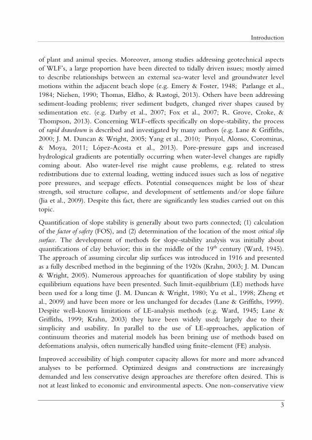
of plant and animal species. Moreover, among studies addressing geotechnical aspects
of WLF’s, a large proportion have been directed to tidally driven issues; mostly aimed
to describe relationships between an external sea-water level and groundwater level
motions within the adjacent beach slope (e.g. Emery & Foster, 1948; Parlange et al.,
1984; Nielsen, 1990; Thomas, Eldho, & Rastogi, 2013). Others have been addressing
sediment-loading problems; river sediment budgets, changed river shapes caused by
sedimentation etc. (e.g. Darby et al., 2007; Fox et al., 2007; R. Grove, Croke, &
Thompson, 2013). Concerning WLF-effects specifically on slope-stability, the process
of rapid drawdown is described and investigated by many authors (e.g. Lane & Griffiths,
2000; J. M. Duncan & Wright, 2005; Yang et al., 2010; Pinyol, Alonso, Corominas,
& Moya, 2011; López-Acosta et al., 2013). Pore-pressure gaps and increased
hydrological gradients are potentially occurring when water-level changes are rapidly
coming about. Also water-level rise might cause problems, e.g. related to stress
redistributions due to external loading, wetting induced issues such as loss of negative
pore pressures, and seepage effects. Potential consequences might be loss of shear
strength, soil structure collapse, and development of settlements and/or slope failure
(Jia et al., 2009). Despite this fact, there are significantly less studies carried out on this
topic.
Quantification of slope stability is generally about two parts connected; (1) calculation
of the factor of safety (FOS), and (2) determination of the location of the most critical slip
surface. The development of methods for slope-stability analysis was initially about
quantifications of clay behavior; this in the middle of the 19th century (Ward, 1945).
The approach of assuming circular slip surfaces was introduced in 1916 and presented
as a fully described method in the beginning of the 1920s (Krahn, 2003; J. M. Duncan
& Wright, 2005). Numerous approaches for quantification of slope stability by using
equilibrium equations have been presented. Such limit-equilibrium (LE) methods have
been used for a long time (J. M. Duncan & Wright, 1980; Yu et al., 1998; Zheng et
al., 2009) and have been more or less unchanged for decades (Lane & Griffiths, 1999).
Despite well-known limitations of LE-analysis methods (e.g. Ward, 1945; Lane &
Griffiths, 1999; Krahn, 2003) they have been widely used; largely due to their
simplicity and usability. In parallel to the use of LE-approaches, application of
continuum theories and material models has been brining use of methods based on
deformations analysis, often numerically handled using finite-element (FE) analysis.
Improved accessibility of high computer capacity allows for more and more advanced
analyses to be performed. Optimized designs and constructions are increasingly
demanded and less conservative design approaches are therefore often desired. This is
not at least linked to economic and environmental aspects. One non-conservative view

Impact of water-level variations on slope stability
4
in slope-stability analysis regards consideration of negative pore pressures in unsaturated
soils. Taking into account negative pore pressures is generally associated with counting
on extra contributions to the shear strength of the soil, resulting in extra slope stability.
Though, there are still many unanswered questions when it comes to effects of
considering peculiarities of unsaturated soil behavior (Sheng et al., 2013).
Due to a worldwide expansion of watercourse regulation, with operational patterns
directly governed by activities of energy balancing and freshwater provision, it is
important to find reliable methods for analysis of stability effects on areas being exposed
to the regulation.
1.2 Objectives
1.2.1 Aim and objectives
The aim of this study is to identify and enlighten potential impacts on waterfront slopes
subjected to water-level fluctuations, including evaluation of methods for slope-
stability analysis.
1. Provide a review of the overall topic, capturing:
Sources of water-level fluctuations and known effects on slope stability
Fundamentals of mechanical properties of coarse grained soils; this with an
emphasis on changes properties.
Advantages and disadvantages of methods available for slope-stability analysis
(applicable to problems focused in this study).
2. Investigate potential impacts on a slope subjected to water-level fluctuations;
this by FEM-modelling.
3. Evaluate approaches for FEM-modelling of impacts on a slope subjected to
water-level fluctuations.
4. Evaluate potential benefits provided by parameter-influence analysis carried out
in modelling work.
Introduction
5
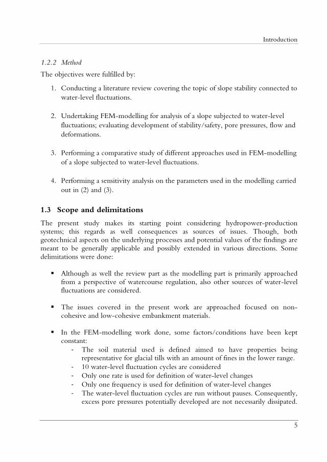
1.2.2 Method
The objectives were fulfilled by:
1. Conducting a literature review covering the topic of slope stability connected to
water-level fluctuations.
2. Undertaking FEM-modelling for analysis of a slope subjected to water-level
fluctuations; evaluating development of stability/safety, pore pressures, flow and
deformations.
3. Performing a comparative study of different approaches used in FEM-modelling
of a slope subjected to water-level fluctuations.
4. Performing a sensitivity analysis on the parameters used in the modelling carried
out in (2) and (3).
1.3 Scope and delimitations
The present study makes its starting point considering hydropower-production
systems; this regards as well consequences as sources of issues. Though, both geotechnical aspects on the underlying processes and potential values of the findings are
meant to be generally applicable and possibly extended in various directions. Some
delimitations were done:
Although as well the review part as the modelling part is primarily approached
from a perspective of watercourse regulation, also other sources of water-level
fluctuations are considered.
The issues covered in the present work are approached focused on non-
cohesive and low-cohesive embankment materials.
In the FEM-modelling work done, some factors/conditions have been kept
constant:
- The soil material used is defined aimed to have properties being representative for glacial tills with an amount of fines in the lower range.
- 10 water-level fluctuation cycles are considered
- Only one rate is used for definition of water-level changes
- Only one frequency is used for definition of water-level changes
- The water-level fluctuation cycles are run without pauses. Consequently, excess pore pressures potentially developed are not necessarily dissipated.
Impact of water-level variations on slope stability
6
This allows for soil conditions to be varying by an increased number of water-level fluctuations run, and also for secondary effects linked to these
non-constant conditions to be captured.
The modelling part is based on a fictive case, i.e. focused on relative changes and differences. Though, input data for the soil model and the hydraulic model
are based on values within ranges found representative. Since the result
evaluation is comparative the exact values of the parameters chosen are not
critical.
1.4 Outline
The introduction (chapter 1) covers the overall background and objectives of the
project. In chapter 2 the essence of the literature review regarding water-level
fluctuations; sources, potential effects on slope stability, and considerations taken, is
found (fully presented in Paper A). Chapter 3 covers some fundamentals on soil
mechanics and slope-stability analysis. In chapter 4 basics of constitutive description of
soils are presented along with details concerning the models used (in Paper B) for
description of as well soil behavior as hydraulic properties. In chapter 5 the modelling
work is described, and in chapter 6 the results are compiled. An overall discussion and
conclusions drawn are presented in chapter 7 and chapter 8, respectively. The
results/outcome from the review work is presented in chapter 7.
Paper A: A review concerning water-level fluctuations; sources, potential geotechnical
effects on slope stability, and considerations taken.
Paper B: A comparative study evaluating different approaches of hydro-mechanical
coupling in FEM-modelling of impacts on a slope subjected to water-level
fluctuations.
Besides what is presented in the present study, involvement in research on
quantification of soil-particle shape has taken place. Work on implementation of 2D-
image analysis on shape quantification was presented in (Rodriguez, Johansson, &
Edeskär, 2012).

Water-level variation – sources, effects, and consideration
7
2 WATER-LEVEL VARIATION – SOURCES, EFFECTS, AND CONSIDERATION
2.1 Sources
2.1.1 Long-term water-level variations
Sea-level rise is one of the most highlighted and debated direct effect of climate
changes. The Bruun-theory (Bruun, 1988) is a generally accepted mathematical model
developed for quantification of relationships between sea-level rise and coastal erosion.
The model is assuming a closed material balance system between the shore and the
offshore bottom profile. This kind of process is actually about the water-soil interface
itself—not necessarily driven by water level changes—but could also be a consequence
of water motion along the course; i.e. streaming/flowing. Though, a varied mean-level
brings changed water-level ranges within which the short-term variations are
occurring. In this sense, a rising sea level acts as an enabler of erosion (K. Zhang et al.,
2004), whereupon consideration also of long-term changes are of importance.
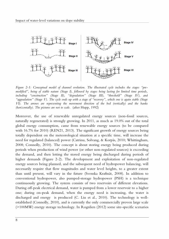
Hupp (1992) presented a channel-evolution cycle in a six-stage model describing the
development from stable conditions, via some time limited landform changing stages,
ending up with another stable state (Figure 2-1).
These examples of long-term effects—as well coastal erosion as channel evolution—are
showing clear consequences of water-soil interaction, entailing obvious effects on
beaches/banks. Though, henceforth short-term water level variations will be focused.
2.1.2 Short-term water-level variations
Energy provision – water storage
In the 1970s, the energy interest grew significantly due to uncertainties related to
provision of oil. This was partly due to a generally spread reluctance to become
dependent on other countries, partly due to concerns about the total global oil reserve
Bardi (2009). The use of energy is growing worldwide; the rate of increased use and
production is high as well in less developed countries, as in industrialized regions.
Impact of water-level variations on slope stability
8
Moreover, the use of renewable unregulated energy sources (non-fossil sources,
naturally regenerated) is strongly growing. In 2011, as much as 19.0% out of the total
global energy consumption, came from renewable energy sources (to be compared
with 16.7% for 2010) (REN21, 2013). The significant growth of energy sources being
totally dependent on the meteorological situation at a specific time, will increase the
need for regulated (balanced) power (Catrinu, Solvang, & Korpås, 2010; Whittingham,
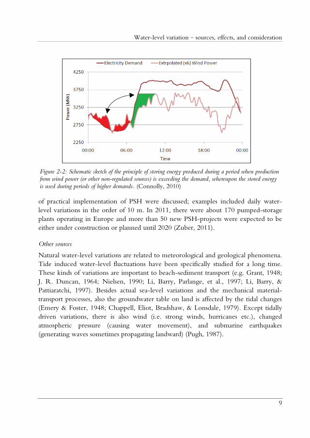
2008; Connolly, 2010). The concept is about storing energy being produced during
periods when production of wind power (or other non-regulated sources) is exceeding
the demand, and then letting the stored energy being discharged during periods of
higher demands (Figure 2-2). The development and exploitation of non-regulated
energy sources being planned, and the subsequent need of hydropower balancing, will
necessarily require that flow magnitudes and water level heights, to a greater extent
than until present, will vary in the future (Svenska Kraftnät, 2008). In addition to
conventional hydropower, also pumped-storage hydropower (PSH) is a technique
continuously growing. The system consists of two reservoirs of different elevations.
During off-peak electrical demand, water is pumped from a lower reservoir to a higher
one; during on-peak demand, when the energy need is increasing, the water is
discharged and energy is produced (C. Liu et al., 2010). The technology is well-
established (Connolly, 2010), and is currently the only commercially proven large scale
(>100MW) energy storage technology. In Rognlien (2012) some site-specific scenarios
Figure 2-1: Co eptual model o ha el evolutio . The illustrated y le i ludes the stages “pre-
modi ied”, bei g o stable ature (Stage I), ollowed by stages bei g lasti g or limited time periods, i ludi g “ o stru tio ” (Stage II), “degradatio ” (Stage III), “threshold” (Stage IV), a d “aggradation” (Stage V). The y le e ds up with a stage o “re overy”, whi h o e is agai stable (Stage VI). The arrows are representing the movement direction of the bed (vertically) and the banks (horizontally). The pictures are not to scale. (after Hupp, 1992)
Water-level variation – sources, effects, and consideration
9
of practical implementation of PSH were discussed; examples included daily water-
level variations in the order of 10 m. In 2011, there were about 170 pumped-storage
plants operating in Europe and more than 50 new PSH-projects were expected to be
either under construction or planned until 2020 (Zuber, 2011).
Other sources
Natural water-level variations are related to meteorological and geological phenomena.
Tide induced water-level fluctuations have been specifically studied for a long time.
These kinds of variations are important to beach-sediment transport (e.g. Grant, 1948;
J. R. Duncan, 1964; Nielsen, 1990; Li, Barry, Parlange, et al., 1997; Li, Barry, &
Pattiaratchi, 1997). Besides actual sea-level variations and the mechanical material-
transport processes, also the groundwater table on land is affected by the tidal changes
(Emery & Foster, 1948; Chappell, Eliot, Bradshaw, & Lonsdale, 1979). Except tidally
driven variations, there is also wind (i.e. strong winds, hurricanes etc.), changed
atmospheric pressure (causing water movement), and submarine earthquakes
(generating waves sometimes propagating landward) (Pugh, 1987).
Figure 2-2: Schematic sketch of the principle of storing energy produced during a period when production from wind power (or other non-regulated sources) is exceeding the demand, whereupon the stored energy is used during periods of higher demands. (Connolly, 2010)

Impact of water-level variations on slope stability
10
2.2 Effects
Drawdown of an external water level is usually impairing the stability of a slope. The
process rapid drawdown is described and investigated by many authors (e.g. Lane &
Griffiths, 2000; J. M. Duncan & Wright, 2005; Yang et al., 2010; Pinyol, Alonso,
Corominas, & Moya, 2011). Pore pressure gaps and increased hydraulic gradients are
potentially occurring as a consequence of rapid water-level changes. Such pore-
pressure gaps combined with a decreased or fully vanished supporting water load, may
lead to reduced slope stability. Studies on this phenomenon have been focused mostly
on earth-fill dams, rather than on waterfront slopes in general. This predominance
notwithstanding, the connection between rapid drawdown, vertical infiltration, and
slope stability was generally highlighted in Yang et al. (2010). The study was based on
laboratory testing of rapid drawdown in a column prepared with two soil layers; clayey
sand over medium sand. Pore-pressure development was logged by time. The soil
properties considered were—besides permeability—specific gravity, liquid limit,
plasticity index, dry density, void ratio, porosity, and water content at saturation. Some
of the results obtained are shown in Figure 2-3; pore pressures plotted against the
depth, with different curves for different times elapsed. The results did clearly confirm
potential outcomes of rapid drawdown; pore pressures remained high and increased
gradients occurred. Consequences of rapid drawdown, including the fact that pore
Figure 2-3: Results from column rapid drawdown tests performed through a soil sample consisting of a
finer soil layer (clayey sand) put over a coarser soil layer (medium sand). Pore-water pressures at different depths (elevations) are plotted at different times. The soil interface is represented by the dotted line. (Yang et al., 2010)
Water-level variation – sources, effects, and consideration
11
pressures are potentially delayed compared to the external water level, have been
shown to be outward seepage, tension cracks developed, and slope failure (Jia et al.,
2009).
Also rising of a water level might cause problems. In studies concerning the Three
Gorges Dam site (e.g. Cojean & Caï, 2011), reduced slope stability has been noticed
during periods of water-level rise. Generally, water-level rise has been shown to cause
stress redistributions due to external loading (as well increases as reductions, in various
directions), wetting induced issues such as loss of negative pore pressures, and seepage
effects. These changes have been shown to cause loss of shear strength, soil structure
collapse, development of settlements, and slope failure. In a large-scale slope model test
reported, with the external water level being varied, vertical settlements at the crest
were noticed (Jia et al., 2009). The deformation development was almost linear during
the first period of water-level rising, and then continuously declining. The vertical
settlements were assigned to wetting-induced soil collapse. Suction values did abruptly
drop immediately when the water level reached the measure points. The horizontal
total stresses were gradually increasing during the rise. In contrast, the vertical stresses
were gradually reduced; asymptotically leveling out until the end of the rise. The
authors suggested that the reduction of vertical stresses were caused by dissipation of
entrapped air, together with gradually reduced stress concentrations (which were
caused by the early observed differential settlements). The settlements were in turn
explained by the wetting; i.e. entrapped air being replaced by water. Loss of negative
pore-pressures and subsequent loss of shear strength did obviously immediately cause
soil structure collapse/failure. Total stress changes were assigned to homogenization of
the slope body; increased horizontal stresses caused by an increased water load, and
vertical stresses stabilized due to stress-concentration dissipation. It was emphasized that
a delayed change of pore pressure inside a slope—relative to the change of the adjacent
external water level—results in significant movements of water within the slope body.
Thus, the seepage forces were found to adversely affect the stability. The seepage-
instability relationship was also confirmed in Tohari, Nishigaki, & Komatsu (2007).
2.3 Consideration
The earliest tools used to take into account different degrees of submergence of a
slope, involved stability charts (Morgenstern, 1963). In the following decades further
investigations were done utilizing limit-equilibrium (LE) methods for expression of
safety factors (Lane & Griffiths, 2000; Huang & Jia, 2009). Later, these kinds of
problems have also been approached using finite-element (FE) tools (e.g. Lane &
Griffiths, 2000; Pinyol et al., 2011).
Impact of water-level variations on slope stability
12
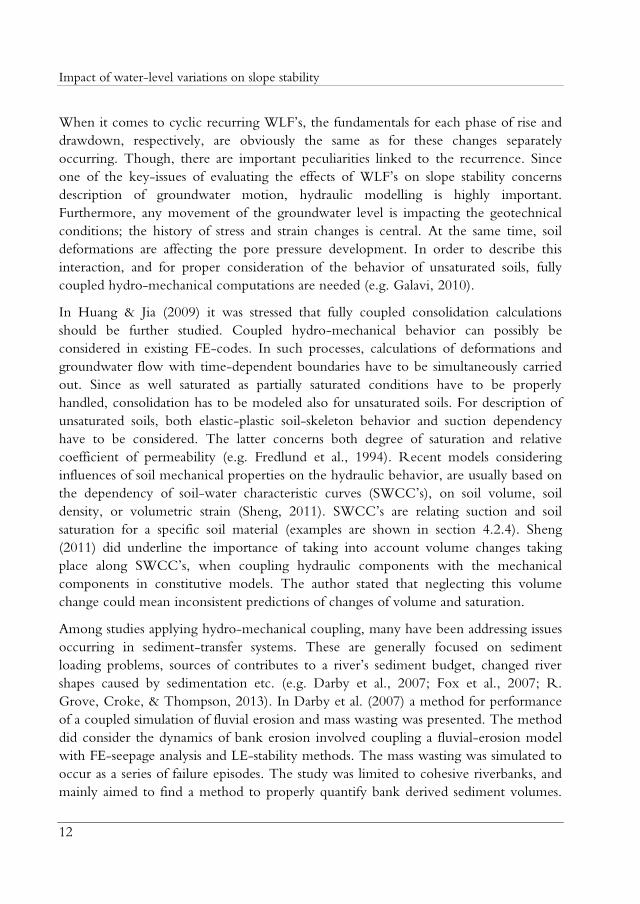
When it comes to cyclic recurring WLF’s, the fundamentals for each phase of rise and
drawdown, respectively, are obviously the same as for these changes separately
occurring. Though, there are important peculiarities linked to the recurrence. Since
one of the key-issues of evaluating the effects of WLF’s on slope stability concerns
description of groundwater motion, hydraulic modelling is highly important.
Furthermore, any movement of the groundwater level is impacting the geotechnical
conditions; the history of stress and strain changes is central. At the same time, soil
deformations are affecting the pore pressure development. In order to describe this
interaction, and for proper consideration of the behavior of unsaturated soils, fully
coupled hydro-mechanical computations are needed (e.g. Galavi, 2010).
In Huang & Jia (2009) it was stressed that fully coupled consolidation calculations
should be further studied. Coupled hydro-mechanical behavior can possibly be
considered in existing FE-codes. In such processes, calculations of deformations and
groundwater flow with time-dependent boundaries have to be simultaneously carried
out. Since as well saturated as partially saturated conditions have to be properly
handled, consolidation has to be modeled also for unsaturated soils. For description of
unsaturated soils, both elastic-plastic soil-skeleton behavior and suction dependency
have to be considered. The latter concerns both degree of saturation and relative
coefficient of permeability (e.g. Fredlund et al., 1994). Recent models considering
influences of soil mechanical properties on the hydraulic behavior, are usually based on
the dependency of soil-water characteristic curves (SWCC’s), on soil volume, soil
density, or volumetric strain (Sheng, 2011). SWCC’s are relating suction and soil
saturation for a specific soil material (examples are shown in section 4.2.4). Sheng
(2011) did underline the importance of taking into account volume changes taking
place along SWCC’s, when coupling hydraulic components with the mechanical
components in constitutive models. The author stated that neglecting this volume
change could mean inconsistent predictions of changes of volume and saturation.
Among studies applying hydro-mechanical coupling, many have been addressing issues
occurring in sediment-transfer systems. These are generally focused on sediment
loading problems, sources of contributes to a river’s sediment budget, changed river
shapes caused by sedimentation etc. (e.g. Darby et al., 2007; Fox et al., 2007; R.
Grove, Croke, & Thompson, 2013). In Darby et al. (2007) a method for performance
of a coupled simulation of fluvial erosion and mass wasting was presented. The method
did consider the dynamics of bank erosion involved coupling a fluvial-erosion model
with FE-seepage analysis and LE-stability methods. The mass wasting was simulated to
occur as a series of failure episodes. The study was limited to cohesive riverbanks, and
mainly aimed to find a method to properly quantify bank derived sediment volumes.
Water-level variation – sources, effects, and consideration
13
Though, the modelling did involve both particle-size characterization and soil-strength
consideration.
The shortfall notwithstanding, some studies on large-scale reservoir fluctuations are
found in the literature. For instance, it was found that the stability of a reservoir slope
consisting of sand and silt, was more directly governed by hydraulic conductivities than
by velocities of water-level changes (Liao et al., 2005). For evaluation of reservoir-
fluctuation effects on a silty slope, the importance of negative pore pressures, friction
resistance, and water-load support was highlighted in Zhan, Zhang, & Chen (2006). In
that study, saturated-unsaturated seepage analysis was combined with LE-stability
analysis. Also in Shen, Zhu, & Yao (2010) examination of “reservoir water-level
fluctuation” did include analysis of only one cycle of rise and drawdown, carried out
by means of LE-calculations. In Galavi (2010) hydro-mechanical theories used in FE-
modelling were presented. Comparisons and evaluations performed showed good
agreement between the results obtained from the numerical FE-computations
performed using the FE-code PLAXIS 2D and those from analytical solutions. In
Kaczmarek & Leśniewska (2011) effects of groundwater-level changes on a flood bank
core were modeled. Stability and seepage were considered by FE-analysis. Though, the
study was only briefly described and neither the input nor the outcomes were
satisfactorily presented.

Impact of water-level variations on slope stability
14

Slope analysis
15
3 SLOPE ANALYSIS
3.1 Introduction
Historically, methods for evaluation or determination of slope stability have been
largely focused on theories regarding fine-grained soils. During the 1840s—related to
the railway construction projects ran at that time—engineers were working on
determination of the shear strength of clay (Ward, 1945). The analysis approach of
assuming circular slip surfaces was introduced in 1916 (Petterson, 1955). Though, a
fully described method was presented by Fellenius in the beginning of the 1920s (e.g.
Krahn, 2003; J. M. Duncan & Wright, 2005). In 1945, Skempton was presenting a
study named “A slip in the west bank of Eau Brink Cut”, including an illustration of a
rotational slip surface within a slope mainly consisting of clay (Ward, 1945).
During the past decades, engineering and research studies have brought knowledge and
formulated theories within the area of soil mechanics. The understanding of different
factors affecting slope stability (e.g. time dependent changes of soil behavior), has been
continuously improved. This not at least due to known limitations of existing methods
for evaluation of soil strength (e.g. laboratory and in situ testing methods) and
development of new tools and instruments for measuring and observing slopes. All this
together has successively formed the now available collection of experience and
knowledge concerning slope behavior and slope failure. This applies for improved
understanding of basic principles of soil mechanics, and improved analysis procedures.
(J. M. Duncan & Wright, 2005)
3.2 Description and classification of soil
The soil skeleton consists of three components. The solids consist of mineral grains
and/or organic constituents. Moreover, free spaces between the solid grains—i.e. the
pores/voids—are exhibiting properties (size and shape) depending on the geometrical
properties of the solids. The pores are filled with fluids (often pore water), gas (often
air), or a mixture of these two. The geotechnical properties of a soil volume are
depending on minerals being present, content of organic material, content of water,
manner of which the water is present, denseness of the soil particle arrangement, and
size and shape of the particles. Different soil types are then grouped with respect to
these characteristics.
Impact of water-level variations on slope stability
16
Soils are usually divided into two main groups; fine-grained soil and coarse-grained soil.
This distinction is based upon the particle sizes; the diameters, d. The fractions clay and
silt are sorted as fine-grained soils, whereas sand and gravel are sorted as coarse-grained
soils. Soils are also classified based upon the kind of forces being contributing to the
soil strength. The grains in purely cohesive soils are held together by van der Walls
forces, hydrogen bonds, and electro-static forces; the resultant makes up cohesive
bonding. On the other hand, the strength of sand and gravel, i.e. frictional soils, is
coming from mechanical inter-granular friction. Silt is sometimes with respect to
strength properties called intermediate soils. (Craig, 2004)
3.3 Stress and strength
3.3.1 Stress
Classical theory
In contrast to fine-grained soils (with strength coming from cohesive forces), the
strength of a coarse grained soil mostly comes from contact forces between the
individual grains. The mass of the soil particles, together with any additional forces
from external loads, are getting normal forces acting at the particle contact areas. The
resultant forces acting on a soil element are to be transmitted through the soil skeleton
components, including also fluids and/or gases. The fundamental and well established
principle of effective stress, , presented by Terzhagi in the 1920th, is expressed as:
where is the total normal stress, and is the pore-water pressure. This equation is
based upon the assumption that there are only two situations; (1) there is a pore
pressure coming from the fully water filled pores, and (2) there is no pore pressure.
Unsaturated soil behavior
In the middle of the 1950th, Bishop proposed an effective stress expression, considering
also partially saturated or unsaturated soils:
( ) (3.2)
where is the pore-air pressure, the pore-water pressure, and an
experimentally determined matric-suction coefficient. This coefficient (Bishop’s
parameter) could be related to the degree of saturation, . The experimental
evidences of are sparse (Galavi, 2010), and the role of the parameter has been
(3.1)

Slope analysis
17
generally questioned (Fredlund, 2006). The often used assumption of letting the
matric-suction coefficient be replaced by the degree of saturation, i.e. , has been
shown to require care to be taken. The validity of the assumption is highly dependent
on the microstructure of the soil type being analyzed; more specifically the fraction of
water filling the micropores, (Pereira et al., 2010). The deviation has been shown
to be higher for fine-grained soils, especially those exhibiting high plasticity. Though,
in PLAXIS (2012) the matric-suction coefficient is substituted with the effective
degree of saturation, . Assuming air-pore pressure is being negligibly low, the
effective stress expression (equation (3.2) becomes:
(3.3)
Unsaturated soil behavior is further discussed in section 4.2.
A number of proposals have been presented aiming to improve the accuracy regarding
definition and description of stress-strain behavior and strength of unsaturated soils.
Limitations of existing effective stress expression were indicated by e.g. Burland &
Jennings (1962). The possibility to control the mechanical response of unsaturated soils
by considering two stress-state variables, namely (1) the net stress, i.e. the difference
between the total stress and the pore-air pressure, and (2) the suction, i.e. the
difference between the pore-air pressure and the pore-water pressure, was firstly
demonstrated by Fredlund & Morgenstern (1977). Moreover, a number of non-linear
elastic constitutive models were developed based upon this. Subsequently, also elastic-
plastic models have been proposed and developed (Sun et al., 2010). Many models are
developed based on the Basic Barcelona Model (Alonso, Gens, & Josa, 1990). The subject
of unsaturated soil was well reviewed in Sheng (2011).
3.3.2 Particle arrangement
At a loose soil-particle arrangement, only a small lateral force is needed to get the soil
particles rearranged into a denser configuration. Therefore, loose soils exhibit low
resistance to volume decrease (contractancy) and deformations. Horizontal shearing of a
dense coarse grained soil sample means stiff and almost elastic initial response. This
since the soil particles of a dense soil are forced to “climb” over each other (in the
direction against the applied vertical load), in order to get a rearrangement taking
place. The soil undergoes volume increase (dilatancy). The response of shear stress, at
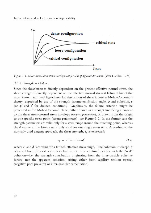
increased shear straining, is conceptually shown in Figure 3-1. When shearing
takes place without any further volume change, the critical state is reached.
Impact of water-level variations on slope stability
18
Figure 3-1: Shear stress/shear strain development for soils of different denseness. (after Hansbo, 1975)
3.3.3 Strength and failure
Since the shear stress is directly dependent on the present effective normal stress, the
shear strength is directly dependent on the effective normal stress at failure. One of the
most known and used hypotheses for description of shear failure is Mohr-Coulomb´s
theory, expressed by use of the strength parameters friction angle, and cohesion,
(or and for drained conditions). Graphically, the failure criterion might be
presented in the Mohr-Coulomb plane; either drawn as a straight line being a tangent
to the shear stress/normal stress envelope (tangent parameters), or drawn from the origin
to one specific stress point (secant parameters), see Figure 3-2. In the former case the
strength parameters are valid only for a stress range around the touching point, whereas
the ´-value in the latter case is only valid for one single stress state. According to the
normally used tangent approach, the shear strength, is expressed:
(3.4)
where c´ and ´ are valid for a limited effective stress range. The cohesion intercept, ’
obtained from the evaluation described is not to be confused neither with the “real”
cohesion—i.e. the strength contribution originating from the inter-particle cohesive
forces—nor the apparent cohesion, arising either from capillary tension stresses
(negative pore pressure) or inter-granular cementation.

Slope analysis
19
Figure 3-2: The bold solid curve connecting the plotted stress points shows the actual shear stress-normal stress combinations of a specific soil. The thin solid line represents the envelope used for tangent approach evaluation of the strength parameters, whereas the dashed line represents the secant approach. (after Craig, 2004)
3.3.4 Angle of internal friction
For a drained granular soil, the total angle of friction—i.e. the angle of friction
mobilized during shearing, —is actually consisting of two main parts:
(3.5)
where is the inter-particle sliding component and the geometrical interference
component. The geometrical component is, in turn, consisting of two parts, namely
coming from the dilation phenomenon (particle climbing), and coming from
particle pushing and rearrangement (Terzaghi et al., 1996).
The final expression is moreover:
(3.6)
3.3.5 Factors governing internal friction – changed properties
Mineral composition and crushing properties
The soil-particle minerals are affecting a coarse-grained soil by two factors; (1) the
friction of the particle surface is directly dependent on the surface roughness (affecting
the sliding component ), (2) the mineral hardness and strength is affecting the
crushing properties of the individual particles (affecting the component ) (Terzaghi
et al., 1996).
Impact of water-level variations on slope stability
20
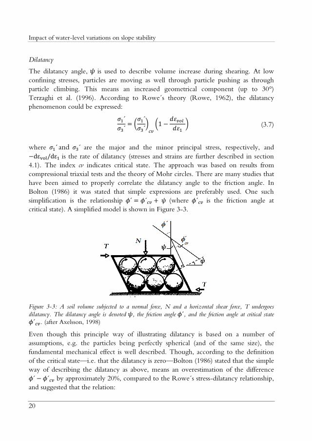
Dilatancy
The dilatancy angle, is used to describe volume increase during shearing. At low
confining stresses, particles are moving as well through particle pushing as through
particle climbing. This means an increased geometrical component (up to 30°)
Terzaghi et al. (1996). According to Rowe´s theory (Rowe, 1962), the dilatancy
phenomenon could be expressed:
(
)
(
) (3.7)
where and are the major and the minor principal stress, respectively, and
is the rate of dilatancy (stresses and strains are further described in section
4.1). The index cv indicates critical state. The approach was based on results from
compressional triaxial tests and the theory of Mohr circles. There are many studies that
have been aimed to properly correlate the dilatancy angle to the friction angle. In
Bolton (1986) it was stated that simple expressions are preferably used. One such
simplification is the relationship (where is the friction angle at
critical state). A simplified model is shown in Figure 3-3.
Figure 3-3: A soil volume subjected to a normal force, N and a horizontal shear force, T undergoes
dilatancy. The dilatancy angle is denoted , the friction angle , and the friction angle at critical state
. (after Axelsson, 1998)
Even though this principle way of illustrating dilatancy is based on a number of
assumptions, e.g. the particles being perfectly spherical (and of the same size), the
fundamental mechanical effect is well described. Though, according to the definition
of the critical state—i.e. that the dilatancy is zero—Bolton (1986) stated that the simple
way of describing the dilatancy as above, means an overestimation of the difference
by approximately 20%, compared to the Rowe´s stress-dilatancy relationship,
and suggested that the relation:
Slope analysis
21
(3.8)
fits Rowe´s stress-dilatancy relationship well. In PLAXIS (2012) the definition of
dilatancy angle is based on Rowe´s theory:
( )
(3.9)
where is the mobilized friction angle and is the friction angle at critial state.
Void ratio and grain size distribution
Depending on to what extent the particles are interlocked and clamped by each other,
the shearing resistance will vary. A simple measure of the soil-skeleton structure is the
void ratio, , defined as the ratio of pore volume, and the volume of the solids, .
At small void ratios of a coarse-grained soil, the total contact area between the particles
is large; the friction angle is high. Therefore, in well-graded soils (e.g. glacial-tills),
where smaller grains are filling the larger voids, friction angles are generally higher than
in poorly graded soils (e.g. uniform sands).
Particle shape
Since Wadell (1932)—one of the first to put attention on how particle shape is
affecting soil behavior—a number of studies have been carried out. In Krumbein
(1941) as well the importance of considering the particle shape, as some methods for
determination and analysis, were discussed. Connections and correlations between
particle shape and mechanical behavior of soils—strength, stiffness/deformations, and
hydraulic properties—are described and discussed in soil mechanics literature (e.g.
Terzaghi et al., 1996; Guimaraes, 2002; Santamarina & Cho, 2004; Mitchell & Soga,
2005; Cho, Dodds, & Santamarina, 2006).
Although there seems to be an agreement regarding the existing influence, the particle
shape is rarely considered in designing of geotechnical structures. Even though particle
shape—as an influencing factor—is mentioned in some guidelines and designing codes,
e.g. Eurocode 7 and RIDAS (Swedenergy, 2008), it is not clearly described how to
actually apply particle-shape information. (Johansson & Vall, 2011)
In literature, the term shape is found to be used some inconsequently and there are
significant variations in how different sub-quantities are used (Johansson & Vall, 2011).
One common approach used for handling the complexity of particle-shape description,
Impact of water-level variations on slope stability
22
is based on three sub-quantities of different geometric scales (Wadell, 1932; Krumbein,
1941; Mitchell & Soga, 2005). At large scale—i.e. when the particle diameters in
different directions are described—the term sphericity is used. At an intermediate
scale—for description of to what extent the particle boundary/perimeter is deviating
from a smooth circle or ellipse—the sub-quantity roundness is used. To describe the
smallest scale of the particle—the texture of the particle surface—roughness is used.
For description of connections between soil-particle shape and the influenced
properties, there are a number of empirical relationships developed. An often seen
expression relating particle shape with strength is:
(3.10)
where v
is the friction angle at critical state, and is a quantity describing the
roundness of the particles. This relation shows that the critical state friction angle is
decreasing with increased roundness of the soil particles (Santamarina & Cho, 2004;
Cho et al., 2006). Also void ratio is depending on the particle shape. At large strains,
when the particle displacements are coming from particle rotation and inter-particle
sliding, the void ratio is decreasing with increased roundness and increased sphericity
(Cho et al., 2006). Since the strength properties are linked to void ratio (and/or
porosity), also this relation affects the strength of the soil. The relevance of
relationships between particle shape and mechanical soil properties, including the
possibility to quantify the shape, was discussed in Rodriguez, Edeskär, & Knutsson
(2013).
3.4 Slope-stability analysis
3.4.1 Introduction
Among the factors causing reduced strength of a soils mass, increased pore pressure is very
important. In addition to pore-pressure increase, also seepage—i.e. water flowing
within the soil—might lead to washing out of soil particles, which moreover cause
undermining of the soil (Ward, 1945). A lot attention has been put on natural events
entailing an upward movement of the groundwater level; e.g. precipitation and
subsequent infiltration (e.g. Lim et al., 1996; Tohari et al., 2007). Another
phenomenon potentially resulting in strength loss is degradation and/or weathering;
physical, chemical, and biological processes breaking down soil particles, rearranging
the structures, and changing the properties of the entire soil mass (J. M. Duncan,
2005).
Slope analysis
23
The slope stability may also get reduced by increased shear stress due to changed loading
conditions. The shear stress could be increased by (1) increased stresses acting in
directions being driving; external loads at the top of the slopes, water pressure in cracks
at the top of the slope, increased soil weight due to increased water content etc. The
shear stress could also be increased by (2) factors making the resistant forces reduced;
any kind of removal of soil at the bottom of the slope, and drop in water level at the
slope base. (J. M. Duncan, 2005)
As mentioned in previous sections, there are different approaches available for
performance of stability analyses; limit-equilibrium methods, and deformation-analysis
methods.
3.4.2 Limit-equilibrium analysis
Limit-equilibrium (LE) methods have been used to analyze slope stability for a long
time (J. M. Duncan & Wright, 1980; Yu et al., 1998; Zheng et al., 2009). These
methods have been unchanged for decades (Lane & Griffiths, 1999). In J. M. Duncan
& Wright (1980) it was emphasized that all equilibrium methods for slope-stability
analysis have some characteristics in common: (1) The factor of safety (FOS) is defined
as the ratio between the shear strength, and the shear stress required for equilibrium,
. Using Mohr-Coulomb’s failure criterion and also applying Terzaghi´s expression for
effective stress, the factor of safety becomes:
( ) ( ) ⁄ (3.11)
where normal stress and pore pressure are denoted and u , respectively, and the
strength parameters friction angle, and cohesion (expressed in terms of effective
stresses, i.e. for drained situations) are denoted by , and , respectively. (2) It is to be
assumed that the stress-strain characteristics of the soils are non-brittle, and that the
same shear-strength value may be mobilized over a wide range of strains along the slip
surface. (3) Some (or all) of the equilibrium equations are used to determine the
average shear stress, and the slip surface normal stress; this in order to possibly use
Mohr-Coulomb’s failure criterion for shear strength calculation. (4) Since the number
of unknowns is larger than the number of equilibrium equations, explicit assumptions
are to be involved.
Among the single free-body procedures, i.e. the group of the LE-method that was first
used, there are in turn sub-procedures being based on different approaches; e.g. the
infinite slope procedure, the logarithmic spiral, and the Swedish circle method. For all of the
single-free body procedures, homogenous soil profiles are preferred. External water

Impact of water-level variations on slope stability
24
levels are considered as external loads, and the groundwater level determines from
what level the soil will get saturated conditions. In Figure 3-4 the principles of some
single free-body limit equilibrium procedures, are shown. In the infinite plane case, the
slope inclination, the soil weight, and the strength parameters are needed for
expression of the factor of safety. For the two other procedures, the shape of the
assumed slip surface, the mass of the soil block bounded by the slip surface and the
ground surface, and the location of the center, are to be determined. (J. M. Duncan &
Wright (2005)
(a) Infinite slope procedure (b) Logarithmic spiral
procedure
(c) Swedish circle procedure
Figure 3-4: Principle sketches of the basics of three single free-body limit-equilibrium procedures. The
ground surfaces, GS and slip surfaces, SS are shown. Moreover, also slope inclination for the infinite
slope case, ; the initial radius, for the logarithmic spiral case; and the constant radius, for the Swedish circle case, are presented.
Slice procedures
Slices procedures were introduced already in the end of the 19th century (Ward, 1945). In
order to simplify the process of determining the driving moments, and to make it
possible to consider slip surfaces of more complex geometries, the soil block could be
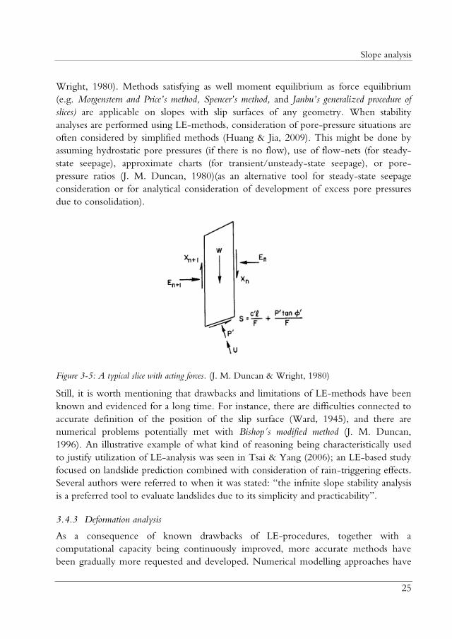
divided into vertical slices. Forces acting on a typical slice are weight, ; shear force
on the slice base, (defined as , where is the shear strength and is the
length of the slice base); effective normal force acting on the base, ; water pressure
force acting on the base, ; vertical side force, ; horizontal side force, (see Figure
3-5).
In the simplest slice procedure, often referred to as the ordinary method of slices, only
overall moment equilibrium is considered. In Bishop´s simplified method also the
equation of vertical force equilibrium of each slice is satisfied; in Bishop´s modified
method, also side forces are considered. All these methods are restricted to circular slip
surfaces. Moreover, there are methods where only the force equilibrium equations are
satisfied; e.g. a method presented by Lowe and Karafiath in 1960 (J. M. Duncan &
Slope analysis
25
Wright, 1980). Methods satisfying as well moment equilibrium as force equilibrium
(e.g. Morgenster a d Pri e’s method, Spe er’s method, and Ja bu’s ge eralized pro edure o
slices) are applicable on slopes with slip surfaces of any geometry. When stability
analyses are performed using LE-methods, consideration of pore-pressure situations are
often considered by simplified methods (Huang & Jia, 2009). This might be done by
assuming hydrostatic pore pressures (if there is no flow), use of flow-nets (for steady-
state seepage), approximate charts (for transient/unsteady-state seepage), or pore-
pressure ratios (J. M. Duncan, 1980)(as an alternative tool for steady-state seepage
consideration or for analytical consideration of development of excess pore pressures
due to consolidation).
Figure 3-5: A typical slice with acting forces. (J. M. Duncan & Wright, 1980)
Still, it is worth mentioning that drawbacks and limitations of LE-methods have been
known and evidenced for a long time. For instance, there are difficulties connected to
accurate definition of the position of the slip surface (Ward, 1945), and there are
numerical problems potentially met with Bishop´s modified method (J. M. Duncan,
1996). An illustrative example of what kind of reasoning being characteristically used
to justify utilization of LE-analysis was seen in Tsai & Yang (2006); an LE-based study
focused on landslide prediction combined with consideration of rain-triggering effects.
Several authors were referred to when it was stated: “the infnite slope stability analysis
is a preferred tool to evaluate landslides due to its simplicity and practicability”.
3.4.3 Deformation analysis
As a consequence of known drawbacks of LE-procedures, together with a
computational capacity being continuously improved, more accurate methods have
been gradually more requested and developed. Numerical modelling approaches have

Impact of water-level variations on slope stability
26
been most widely used based on finite-element (FE) methods; applied to the field of
soil mechanics in the 1960s (J. M. Duncan, 1996). When using FE-methods the
volume/area being analyzed is considered as a continuum whereupon it is discretized
to a finite number of sub-volumes/sub-areas (elements) forming a mesh. In contrast to
the fundamentals of LE-methods, a system analyzed with deformations-analysis
approaches is not considered to necessarily be in equilibrium; neither in terms of forces
nor moments. Besides consideration of stresses and geometrical conditions, stress-strain
relationships are to be described. This is done by use of constitutive models considering
different material properties. Moreover, the key-issue is to as reliably as possible define
these constitutive relationships for a certain soil.
When it comes to definition of stability in terms of safety factors, a procedure of
simulating reduced strength until failure occurs is used. This method was firstly used in
the 1970s (Zheng et al., 2009) and is usually referred to as the shear strength reduction
technique. In PLAXIS 2D 2012 this is mathematically handled by expressing ratios of
the strength parameters:
(3.12)
where is a controlling multiplier representing the safety factor; is the cohesion;
is the friction angle; and the index reduced indicates values being successively
decreased until failure occurs. For indication of global instability of soil slopes, the non-
convergence of solutions is often used. This is indicated by the condition when a stress state at which the failure criterion and the global equilibrium can be simultaneously
satisfied, is not found (Lane & Griffiths, 2000).
The method is usable for constitutive models utilizing strength parameters that can be
reduced. The safety factor is principally defined as in LE-approaches, i.e. by the ratio
between the available shear strength and the shear stress at failure.
3.4.4 Drainage conditions
Since soil strength is directly dependent on the presence of water and the interaction
between the soil and the water, consideration of draining conditions is crucial for proper
evaluation of different soil-mechanical behavior patterns. In a situation with fixed
conditions—i.e. concerning water level, loading, inherent soil properties, and
geometry—the pore pressure is hydrostatic. At occurrence of any changes, the pore-
pressure situation is potentially affected. In coarse-grained soils, water is easily moving.

Slope analysis
27
This means that loading could be allowed without the pore-pressure state being
changed; drained analysis is performed. In fine-grained soils, low permeability might
mean a rate of drainage being lower than the rate of total stress change, meaning
potential development of increased (excess, non-hydrostatic) pore pressures.
Analogously, this could also be the case in coarse-grained soil if the total-stress is
changed rapidly enough. In the two latter situations, undrained analysis is to be
performed. Depending on what kinds of changes being expected and for what time-
perspective the stability is assessed, either drained or undrained conditions are most
critical. Therefore, both cases are to be considered; combined analysis is performed.

Impact of water-level variations on slope stability
28
Modelling of soil and water
29
4 MODELLING OF SOIL AND WATER
4.1 Constitutive description of soil
4.1.1 Stress
For each specific stress state there are orthogonal stress directions in which the normal
stresses display their maximum and minimum values; principal stresses, acting in the
principal stresses directions. At the planes directed perpendicular to the principal stress
directions, no shear stresses are acting. In two-dimensional (plane stress) situations there
are two principal stresses; the major principal stress, and the minor principal stress,
. In a three-dimensional situation the minor stress is denoted , and the
intermediate principal stress gets the denotation .
The average value of the principal stresses acting in a specific point within the soil mass
is governing the volume change of a soil unit. It is termed mean pressure, p´, expressed
as:
( ) (4.1)
The stress measure deviatoric stress is governing the shape change of a soil volume, for
the triaxial case expressed :
√
(
) (4.2)
where , and are the deviatoric normal stresses components; each defined as the
difference between the mean pressure and the corresponding principal stress.
4.1.2 Strain
Normal strain, which indicates the displacement in a specific direction, e.g. in the x-
direction, is—according to engineering notations—defined as:

Impact of water-level variations on slope stability
30
(4.3)
where is the strain, is the displacement, and is the initial length. Strains in
other directions are analogously expressed. The shear strains are moreover (for small
strains)—again according to engineering notation—determined by summing the ratios
of displacements and initial dimensions perpendicular to the measured displacements,
e.g.:
⁄ ⁄ (4.4)
where is the shear strain component in the x:y-plane, is the displacement
in the direction perpendicular to the length/dimension , ( and analogously
related).
In order to capture volume changes governed by isotropic compression, the volumetric
strain increment, is expressed as:
(4.5)
where the ratio of a negative change of the specific volume, and the initial
specific volume, , is defined as a positive volumetric strain. Specific volume is
defined as (where is the void ratio). The total volumetric strain is
expressed as a sum of the principal strains ( ) or as a ratio of the
volume change and the total volume ( ⁄ ).
Deviatoric normal strains are associated with shape changes. In the x-direction, is
expressed as:
(4.6)
with the variables defined above. Deviatoric normal strains in other directions are
analogously expressed. In case of triaxial loading—with an axial strain, deviating
from the two radial strains , the deviatoric axial strain, (also denoted ) becomes:
( )
(4.7)
4.1.3 Elastic response
Stress-strain relationships for a soil are different for compression (volume change) and
shearing (shape change). At axial or isotropic compression, axial (index: a) and/or
Modelling of soil and water
31
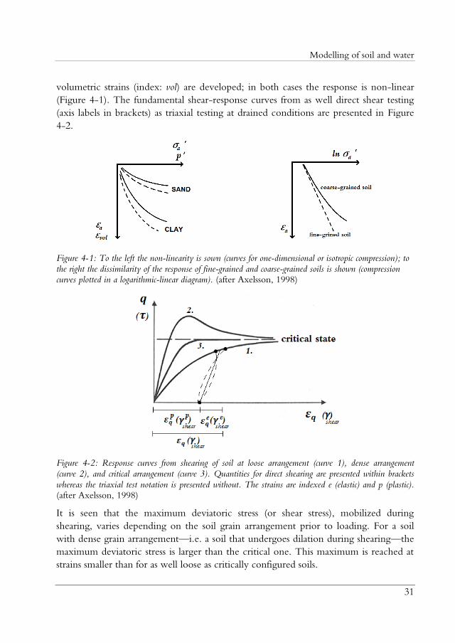
volumetric strains (index: vol) are developed; in both cases the response is non-linear
(Figure 4-1). The fundamental shear-response curves from as well direct shear testing
(axis labels in brackets) as triaxial testing at drained conditions are presented in Figure
4-2.
Figure 4-1: To the left the non-linearity is sown (curves for one-dimensional or isotropic compression); to the right the dissimilarity of the response of fine-grained and coarse-grained soils is shown (compression curves plotted in a logarithmic-linear diagram). (after Axelsson, 1998)
Figure 4-2: Response curves from shearing of soil at loose arrangement (curve 1), dense arrangement (curve 2), and critical arrangement (curve 3). Quantities for direct shearing are presented within brackets
whereas the triaxial test notation is presented without. The strains are indexed e (elastic) and p (plastic). (after Axelsson, 1998)
It is seen that the maximum deviatoric stress (or shear stress), mobilized during
shearing, varies depending on the soil grain arrangement prior to loading. For a soil
with dense grain arrangement—i.e. a soil that undergoes dilation during shearing—the
maximum deviatoric stress is larger than the critical one. This maximum is reached at
strains smaller than for as well loose as critically configured soils.

Impact of water-level variations on slope stability
32
The resistance against elastic straining is described by stiffness moduli. The description
used in the Mohr-Coulomb’s elastic-perfectly plastic model, is presented in section
4.1.6.
4.1.4 Unloading/reloading
Once a soil is unloaded, it will undergo swelling (corresponding to elastic
deformations). The subsequent reloading of the same soil will result in a stress-strain
response that coincides with the unloading path. To curve 1 in Figure 4-2 an
unloading/reloading-curve (dashed), and a straight line that approximately represents
the unloading/reloading-curve, is added.
4.1.5 Plastic response
For stresses high enough, compression or shearing of a soil ends up with irreversible
(plastic) strains. In such a situation, the total strains developed due to loading consist of
as well elastic as plastic strain contributions (see Figure 4-2). The response is therefore
said to be elastic-plastic. In the x-direction this is expressed as:
(4.8)
where the total strain increment, consists of the elastic increment, and the
plastic increment,
. The strain increments in other directions are analogously
expressed.
The soil behavior related to elastic-plastic deformation is captured by the theory of
plasticity. In order to properly take into account both elastic and plastic strains when
analyzing or modelling soil behavior, the stress states at which plastic strains are
developed, have to be defined. This limit—the yield criterion—is expressed by a yield
function, f defining the stress limits in one, two, or multiple dimensions. For instance,
regarding one-dimensional (or isotropic) compression, the yield function is depending
on the effective mean pressure, ; more specifically the preconsolidation pressure, .
For stresses higher than the preconsolidation pressure, there will be plastic strains
developed. For multiaxial stress states, the yield functions can be expressed as e.g.
( ) or ( ) Geometrically, the yield criteria in the stress plane
and the stress space are represented by a yield locus, and a yield surface, respectively. The
yield criteria are expressed in different ways in different elastic-plastic constitutive
models. Though, stress states entailing yield function values mean development
of only elastic deformations. For these states the strains are determined using elastic
stiffness moduli, in addition to values of mean stress and deviatoric stress.

Modelling of soil and water
33
At stress states causing the yield criteria being reached ( )—i.e. when plastic strains
are developed—the strain magnitude is to be determined using a flow rule based on the
gradient of the so called plastic potential function, . Moreover, the plastic strain increment,
is expressed as a function of the partial differential of the plastic potential function,
(differentiated with respect to the stress). Depending on the type of deformation
being of interest, the strain increments are expressed in different ways. In Table 4-1
common strain-increment expressions are presented; including the plastic potential
functions related to each expression.
Table 4-1: Strain-increment expressions and plastic potential functions for different stress quantities. The plastic potential functions contain at least the variables presented in the table.
Stress quantity Strain
increment 1) Plastic potential function, 2)
Normal stress
(engineering notation)
( )
3)
Normal stress
(tensor notation)
( )
4)
Mean pressure
( )
Deviatoric stress
( )
1) The plastic multiplier, determines the magnitude of the plastic straining. 2) The plastic potential functions are depending on at least the variables presented in the table.
Different constitutive models may involve addition variables. 3) Increments in other directions are analogously expressed by substitution of x. 4) General tensor notation. The partial differential of the plastic potential function is determining
the direction of plastic straining.
Since as well the yield function as the plastic potential function are functions of the
stress state, there might be cases when . This special case is termed associated flow.
This kind of flow is used when contractancy response is significant (e.g. in normally
consolidated clays). Still, the general case—when , i.e. non-associated flow—is
frequently used to describe the behavior of coarse-grained soil where both
contractancy and dilatancy are possibly occurring.
For elastic-plastic models there are different approaches for definition of the yield
function. The classical way of describing elastic-plasticity is based on so called elastic-
perfectly plastic theory. In these approaches the yield functions are assumed to be fixed,
i.e. not influenced by the plastic straining itself. In contrast to this, there are also more
sophisticated models which are considering yield property changes related to

Impact of water-level variations on slope stability
34
development of plastic strains. As a consequence of strain dependency of the yield
function, the stress limit at which plastic strains are initiated, changes. This means that
the elastic range will either grow or shrink as a result of developed plastic strains. For as
well one-dimensional as isotropic compression, hardening (grown elastic range) is
simply described by an increased preconsolidation pressure, . This means that the
yield function is also dependent on this quantity, i.e. ( ).
Time dependent strain
In order to fully describe plastic yielding, time related phenomena are to be
considered. This kind of yielding—i.e. permanent deformations developed over time,
under constant effective stresses—is usually referred to as creep. In Tatsuoka (2007) it
was emphasized that an increment of plastic strain, is caused by three phenomena;
(1) plastic yielding, (2) viscous deformation (i.e. time-dependent yielding), and (3)
inviscid cyclic loading effect. usually called creep. Historically, the viscous deformation
part (creep) has mostly been considered as an issue in fine-grained soils; especially in
highly plastic clays. For fine-grained soils creep is mainly caused by volumetric
yielding; usually explained by “secondary consolidation”. However, when it comes to
coarse-grained soils—i.e. where the deformations are mainly caused by shear
yielding—the research has been relatively limited. The lack of studies performed on
sand has been noticed and expressed by many authors, e.g. Murayama, Michihiro, &
Sakagami (1984), Lade & Liu (1998) and Kuwano & Jardine (2002).
Though, in the late 70s and early 80s, some researchers were carrying out experimental
studies on creep characteristics of sand. Rheological models were formulated and
evaluated, and it was suggested that creep behavior of sands could be expressed in
terms of stresses and stress ratios; the findings were presented in e.g. Murayama et al.
(1984). During recent years there have been some more studies carried out on time-
dependent deformation on coarse-grained soils. Kuhn & Mitchell (1993) did propose a
distinction to be made between two main groups of mechanisms to be considered
when it comes to creep rate changing with time; deformation-dependent mechanisms and
intrinsically time-dependent processes. Di Benedetto, Tatsuoka, & Ishihara (2002) presented
how to consider also viscosity (i.e. creep behavior) in an elastic-plastic model used for
description of the behavior of sand. As a fundamental part of the model presented, a
distinction was made not only between elastic and plastic strains, but also between
time-independent and time-dependent stresses. The instantaneous stress, was
expressed as:
(4.9)
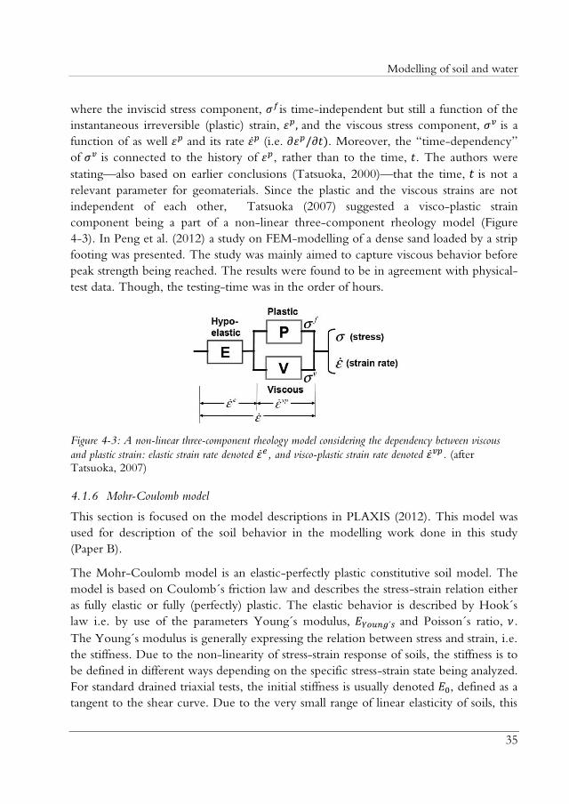
Modelling of soil and water
35
where the inviscid stress component, is time-independent but still a function of the
instantaneous irreversible (plastic) strain, and the viscous stress component, is a
function of as well and its rate (i.e. ). Moreover, the “time-dependency”
of is connected to the history of , rather than to the time, . The authors were
stating—also based on earlier conclusions (Tatsuoka, 2000)—that the time, is not a
relevant parameter for geomaterials. Since the plastic and the viscous strains are not
independent of each other, Tatsuoka (2007) suggested a visco-plastic strain
component being a part of a non-linear three-component rheology model (Figure
4-3). In Peng et al. (2012) a study on FEM-modelling of a dense sand loaded by a strip
footing was presented. The study was mainly aimed to capture viscous behavior before
peak strength being reached. The results were found to be in agreement with physical-
test data. Though, the testing-time was in the order of hours.
Figure 4-3: A non-linear three-component rheology model considering the dependency between viscous
and plastic strain: elastic strain rate denoted , and visco-plastic strain rate denoted . (after Tatsuoka, 2007)
4.1.6 Mohr-Coulomb model
This section is focused on the model descriptions in PLAXIS (2012). This model was
used for description of the soil behavior in the modelling work done in this study
(Paper B).
The Mohr-Coulomb model is an elastic-perfectly plastic constitutive soil model. The
model is based on Coulomb´s friction law and describes the stress-strain relation either
as fully elastic or fully (perfectly) plastic. The elastic behavior is described by Hook´s
law i.e. by use of the parameters Young´s modulus, and Poisson´s ratio, .
The Young´s modulus is generally expressing the relation between stress and strain, i.e.
the stiffness. Due to the non-linearity of stress-strain response of soils, the stiffness is to
be defined in different ways depending on the specific stress-strain state being analyzed.
For standard drained triaxial tests, the initial stiffness is usually denoted , defined as a
tangent to the shear curve. Due to the very small range of linear elasticity of soils, this

Impact of water-level variations on slope stability
36
modulus is not properly describing the stiffness of loaded soils. Therefore, the modulus
is instead used. This is a secant modulus intersecting the shear curve at the
deviatoric stress corresponding to 50% of the peak value. Moreover, elastic
unloading/reloading is described by the modulus . In Figure 4-4, the definitions of
the moduli are principally shown.
Figure 4-4: The initial stiffness , the often used secant stiffness, , and the unloading/reloading
stiffness, , defined. The unloading/reloading curve is represented with the long-dashed line. (modified after PLAXIS, 2012)
Poisson´s ratio, expresses the ratio of strains developed perpendicularly to each other.
For triaxial compression, the parameter expresses the ratio between lateral and axial
strains. For one-dimensional compression, the relationship between Poisson´s ratio,
and the horizontal and vertical effective stresses, is expressed as:
(4.10)
The stiffness can alternatively be described and defined by the shear modulus,
defined as:
( ) (4.11)
or by the oedometer modulus, defined as:
( )
( )( ) (4.12)
Modelling of soil and water
37
Since the failure line defines the ultimate state up to which the developed strains are
elastic, this fixed line is also representing the yield function, separating the two types of
strain response (elastic and plastic). The full three-dimensional yield criterion consists
of six yield functions; two functions in each plane of stress pairs. In terms of principal
stresses, and with the major and the minor principal stresses ( and ), the yield
functions are expressed as:
( )
( ) ( ) ( ) (4.13)
and
( )
( ) ( ) ( ) (4.14)
Moreover, there are another four equations needed (analogously expressed, with all
combinations of and ) to fully define the yield surface in three dimensions.
The surface has the shape of a hexagonal cone, illustrated in Figure 4-5.
In the plastic potential functions, which are parts of the flow rule (see Table 4-1) an
additional plasticity parameter is used; the dilatancy angle, (discussed in section
3.3.5). The plastic potential functions are expressed as:
( )
( ) ( ) (4.15)
and
( )
( ) ( ) (4.16)
Moreover, there are another four equations needed (analogously expressed, with all
combinations of and ) for definition the whole yield surface.
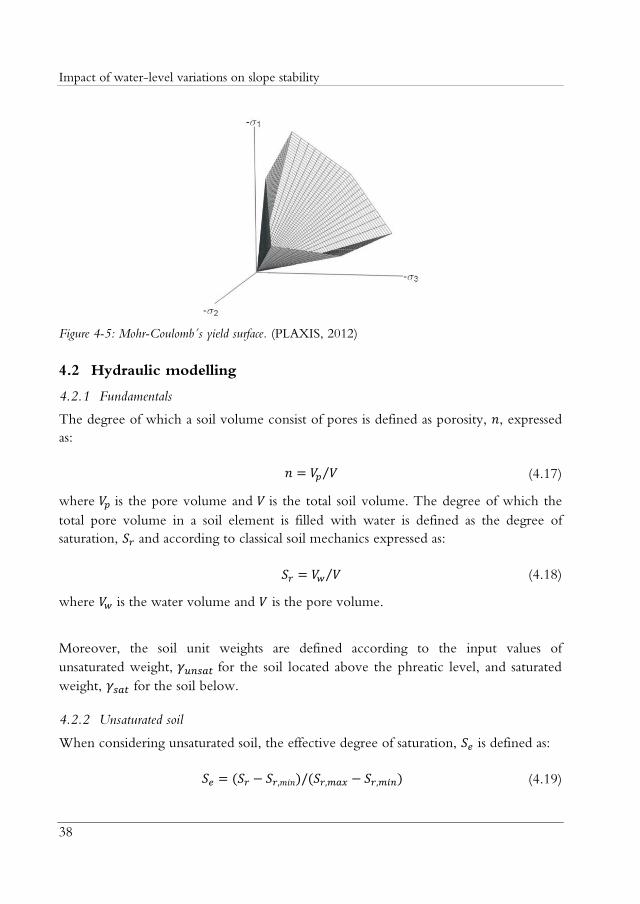
Impact of water-level variations on slope stability
38
Figure 4-5: Mohr-Coulomb´s yield surface. (PLAXIS, 2012)
4.2 Hydraulic modelling
4.2.1 Fundamentals
The degree of which a soil volume consist of pores is defined as porosity, , expressed
as:
⁄ (4.17)
where is the pore volume and is the total soil volume. The degree of which the
total pore volume in a soil element is filled with water is defined as the degree of
saturation, and according to classical soil mechanics expressed as:
⁄ (4.18)
where is the water volume and is the pore volume.
Moreover, the soil unit weights are defined according to the input values of
unsaturated weight, for the soil located above the phreatic level, and saturated
weight, for the soil below.
4.2.2 Unsaturated soil
When considering unsaturated soil, the effective degree of saturation, is defined as:
( ) ( ) (4.19)
Modelling of soil and water
39
where is the degree of saturation and the indices max and min denote maximum and
minimum values. The effective degree of saturation is used also for definition of actual
soil unit weight, :
( )
(4.20)
where the indices denote unsaturated and saturated conditions.
4.2.3 Flow
The rate of water flow, in saturated soil is according to Darcy´s law defined as:
(4.21)
where is the hydraulic gradient (defined as the ratio between head loss, and the
flow length ), ( ⁄ ), is the water density, is the acceleration of
gravity, is the intrinsic permeability, and is the dynamic viscosity of the fluid (the
water).
In unsaturated soils, the hydraulic conductivity is reduced due to air present in the
pores. This reduction is in PLAXIS 2D 2012 (Galavi, 2010) considered by expressing
the specific discharge, , as:
( ) (4.22)
where is the gradient of the pore pressure causing the flow; is the vector of
acceleration of gravity; and is the relative permeability, defined as:
⁄ (4.23)
where is the tensor of permeability at a given saturation. Moreover, is in van
Genuchten model computed according to the dependency on , see equation (4.27).
Starting with the continuity equation—involving mass concentration ( ) and the
divergence of the mass flux density of the residual water ( )—neglecting the
compression of the solid particles as well as of the overall soil structure, the expression
for transient flow becomes:
Impact of water-level variations on slope stability
40
(
)
[
( )] (4.24)
where is the bulk modulus of water, and other parameters as above. In case of
steady-state flow there is no time dependence of the pore-pressure change, whereupon
the left term in equation (4.24) is eliminated.
4.2.4 van Genuchten model
For description of hydraulic behavior in the soil, va Ge u hte ’s model (van
Genuchten, 1980) was used in the modelling work done in this study (Paper B).
The important role of the hydraulic model is to properly define the degree of
saturation, as a function of suction pore-pressure head, . This relation is expressed
as:
( ) ( )[ ( | |)
] (4.25)
where is the residual degree of saturation, is the saturated degree of saturation,
is an empirical parameter describing air entry, and is an empirical parameter
related to the water extraction from the soil (Galavi, 2010). The suction pore pressure
head is defined as:
⁄ (4.26)
where is the suction pore pressure and is the weight of the water. The relative
permeability is expressed as:
( ) [ (
)
]
(4.27)
where is an empirical parameter. The hydraulic properties of a soil are often
presented in soil-water characteristic curves (SWCC). In Figure 4-6 and Figure 4-7,
SWCC’s for different values of the empirical parameters in van Genuchten´s hydraulic
model are shown.
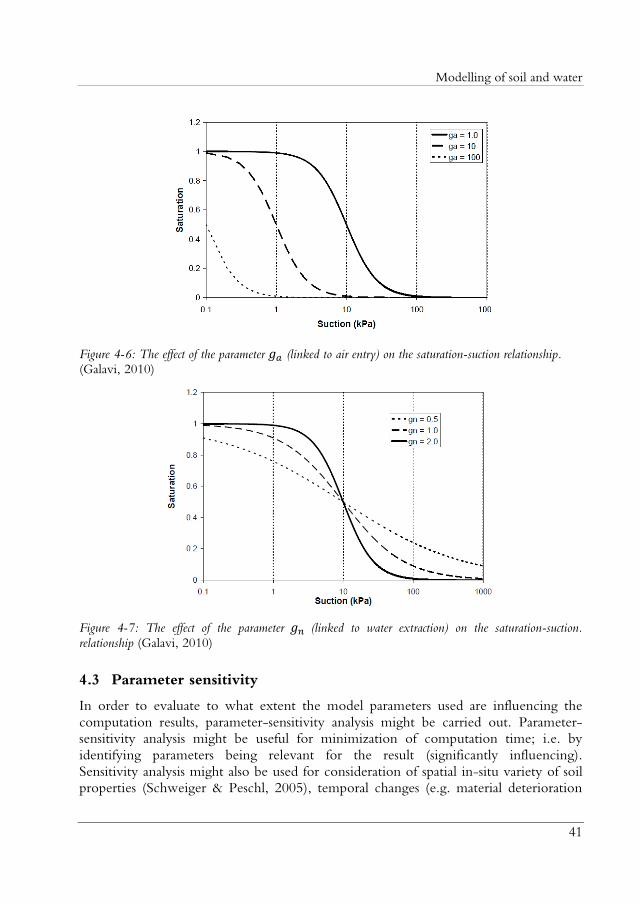
Modelling of soil and water
41
Figure 4-6: The effect of the parameter (linked to air entry) on the saturation-suction relationship. (Galavi, 2010)
Figure 4-7: The effect of the parameter (linked to water extraction) on the saturation-suction. relationship (Galavi, 2010)
4.3 Parameter sensitivity
In order to evaluate to what extent the model parameters used are influencing the
computation results, parameter-sensitivity analysis might be carried out. Parameter-sensitivity analysis might be useful for minimization of computation time; i.e. by
identifying parameters being relevant for the result (significantly influencing).
Sensitivity analysis might also be used for consideration of spatial in-situ variety of soil properties (Schweiger & Peschl, 2005), temporal changes (e.g. material deterioration
Impact of water-level variations on slope stability
42
due to loading and aging), and/or uncertainties connected to the actual quantification (e.g. laboratory tests and field tests).
In the stability-modelling performed in this study (Paper B), sensitivity analysis was
used for comparison of the three analysis approaches evaluated. The parameter
influence was investigated with respect to changed stability (FOS). For each parameter, a maximum and a minimum value were defined setting up an interval within which
the reference value for each parameter was located. The theories used are based on the
ratio of the percentage change of the result, and the percentage change of input
(creating the output change); explained in e.g. U.S. EPA (1999). The sensitivity ratio –sometimes called elasticity (e.g. U.S. EPA, 2001)—is expressed as:
( ( ) ( )
( )) (
)⁄ (4.28)
where the output values are functions, of the input values , for which no index
represents the reference input values and the indices U,L represents the changed ones;
upper/lower. In order to increase the robustness of the analysis (PLAXIS, 2012) the
sensitivity ratio was weighted by a normalized variability measure. This was done using
a sensitivity score, , defined as the ratio of the range itself (or the standard deviation)
and the reference value (U.S. EPA, 2001):
(
) (4.29)
where and defines the range limits, and is the mean (reference) value.
The total sensitivity was then calculated as:
(
∑ ( )) (4.30)
where and
are the sensitivity scores connected to the upper and lower
parameter value, respectively, and ∑ is the sum the sensitivity scores of all
parameter combinations. Five model parameters were considered. In addition to the
reference computation, one computation was run for each range boundary for each
parameter (keeping the other parameters fixed), meaning 11 computations per stability
case.

FEM-Modelling
43
5 FEM-MODELLING
5.1 Main aim
The modelling work done (Paper B) was aimed to (1) investigate potential impacts on
watercourse slopes subjected to recurring water-level fluctuations, (2) to find out
whether there are important dissimilarities between a well-established modelling
approach (based on the classical theory of saturated soil) and approaches that also
consider unsaturated soil behavior, and (3) to analyze potential parameter-influence
changes coming from the water-level changes. More details are presented in Paper B.
5.2 Strategy
The following modelling strategies were used:
Approach 1 (A1): Computations were performed using Terzaghi's definition of stress.
Flow computations were run prior to the deformation computations; the results were
then used in the deformation computations for the corresponding time step. The
consolidation computations were based on excess pore pressures.
Approach 2 (A2): For the fully coupled approach Bishop’s effective-stress equation was
used. The consolidation computations were based on the Biot’s theory of consolidation
(Biot, 1941); i.e. using total pore pressures with no distinction made between steady
state and excess pore pressures.
Approach 3 (A3): Computations were run like in A2, but with stability computations
run without consideration of negative pore pressures.
A fictive waterfront bank slope consisting of a well-graded postglacial till was simulated
to be subjected to a series of water-level-fluctuation cycles (WLFC’s). Development of
stability (in terms of factors of safety, FOS), vertical displacements, pore pressures, flow,
and model-parameter influence, was investigated for an increased number of WLFC’s.
The modelling was performed by use of the software PLAXIS 2D 2012 (PLAXIS,
2012), allowing for consideration of transient flow and performance of coupled hydro-
mechanical computations. This FEM-code was used since it is well-established, and
providing what is needed. Moreover, parameter-influence analysis was performed with

Impact of water-level variations on slope stability
44
respect to FOS’s computed using the strength reduction technique. The parameter-
influence development with an increased number of WLFC’s, was investigated.
The bank was assumed to be infinite in the direction perpendicular to the model plane;
i.e. 2D plain-strain conditions were assumed. The initial stress situation was
determined by a Gravity loading computation; providing initial stresses generated based
on the volumetric weight of the soil (this since the non-horizontal upper model
boundary means that the K0-procedure is not suitable). Then a plastic nil-step was run,
solving existing out-of-balance forces and restoring stress equilibrium. The WLFC’s
were defined in separate calculation steps; one drawdown-rise cycle in each. Each
WLFC was followed by a FOS-computation. In A3, each FOS-computation was
preceded by a plastic nil-step; this to reset the stress situation in order to omit
consideration of negative pore pressures. Sensitivity analysis was carried out for the
three approaches. Five parameters were considered. Ranges used are presented in
Table 5-2.
5.3 Geometry, materials, and definition of changes
The model geometry was defined aimed to represent one half of a watercourse cross
section. The model dimensions and mesh conditions were defined aimed to avoid (1)
errors due to disturbances by the boundaries (due to too small model), (2) errors due to
too coarse mesh, and (3) unreasonably time consuming computations due to too fine
mesh. The slope height was set to 30 m, and the slope inclination to 1:2 (26.6°)
(Figure 5-1); both measures considered to be representative for a watercourse slope
consisting of a well-graded postglacial till, for Swedish conditions (properties presented
in Table 5-1). 15-noded triangular elements were used. The mesh density was
optimized by mesh quality checks done with the built in tool available in PLAXIS
(2012) (the average element quality was 97%). Since the area around the position
where the slope face and the external water level intersect was assumed to be most
critical, extra care was taken regarding mesh density and quality in this region.
The vertical model boundaries were set to be horizontally fixed and free to move
vertically, whereas the bottom boundary was completely fixed. The left vertical
boundary was assumed to have properties of a symmetry line, and the model bottom to
represent a material being dense and stiff relative to the soil above. Therefore, as well
the left vertical hydraulic boundary as the horizontal bottom, were defined as closed
(impermeable). The right vertical boundary was defined to be assigned pore pressures
by the head, simulating allowed in/out flow. Data-collection points were placed where
interesting changes would be expected; at the crest, down along the slope surface, and

FEM-Modelling
45
along a vertical line below the crest. The initial water-level position was set to
+22.0 m (with the level of the watercourse bottom at ± 0 m), the level-change
magnitude to 5.0 m (linearly lowered and raised), and the rate to 1.0 m/day. The
water-level changes were run continuously; i.e. without allowing pore pressures to
even out. Since the study was comparative, this was not mainly intended to reflect
frequently occurring real situations.
5.4 Models used
The soil was described using Mohr Coulomb´s model. This model was chosen for
three reasons; (1) it is well-established and widely used by engineers, (2) as soon as the
stability analysis is started (performed using the strength reduction technique), any
model defined with the same strength parameters would behave like the Mohr-
Coulomb model (i.e. stress dependent stiffness is excluded), (3) the study is
comparative whereupon differences between the modelling approaches evaluated were
focused rather than the accuracy of the soil description.
The hydraulic properties were defined using the van Genuchten´s model (van
Genuchten, 1980). The model is widely recognized and integrated in PLAXIS.
Both models were described in chapter 4.
Figure 5-1: Model geometry. Dimensions, initial water level (𝑊𝐿𝑖𝑛𝑖𝑡𝑖𝑎𝑙), and the pre-defined data-collection points (A) at the crest, and (B) at the level +22 m, are shown in the figure.
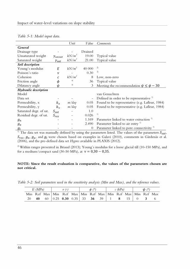
Impact of water-level variations on slope stability
46
Table 5-1: Model input data.
Unit Value Comments
General
Drainage type - - Drained
Unsaturated weight kN/m3 19.00 Typical value
Saturated weight kN/m3 21.00 Typical value
Soil description
Young´s modulus kN/m2 40 000 2)
Poisson´s ratio - 0.30 2)
Cohesion kN/m2 8 Low, non-zero
Friction angle ° 36 Typical value
Dilatancy angle ° 3 Meeting the recommendation
Hydraulic description
Model
van Genuchten
Data set - - - Defined in order to be representative 1)
Permeability, x m/day 0.05 Found to be representative (e.g. Lafleur, 1984)
Permeability, y m/day 0.05 Found to be representative (e.g. Lafleur, 1984)
Saturated degr. of sat. - 1.0
Residual degr. of sat. - 0.026 1)
- - 1.169 Parameter linked to water extraction 1)
- - 2.490 Parameter linked to air entry 1)
- - 0 Parameter linked to pore connectivity 1) 1) The data set was manually defined by using the parameters listed. The values of the parameters ,
, , , and were chosen based on examples in Galavi (2010), comments in Gärdenäs et al. (2006), and the pre-defined data set Hypres available in PLAXIS (2012).
2) Within ranges presented in Briaud (2013); Young´s modulus for a loose glacial till (10-150 MPa), and
for a medium/compact sand (30-50 MPa), at .
NOTE: Since the result evaluation is comparative, the values of the parameters chosen are not critical.
Table 5-2: Soil parameters used in the sensitivity analysis (Min and Max), and the reference values.
E (MPa) v (-) (°) c (kPa) (°)
Min Ref Max Min Ref Max Min Ref Max Min Ref Max Min Ref Max
20 40 60 0.25 0.30 0.35 33 36 39 1 8 15 0 3 6

Results and comments
47
6 RESULTS AND COMMENTS
6.1 Evaluation of FEM-modelling approaches
6.1.1 General
More details are presented in Paper B.
6.1.2 Stability
In Figure 6-1 the failure plots from the three modelling approaches are shown;
conditions at the initial stage (Init.), after one rapid drawdown (RDD), and after one
WLFC (1); corresponding FOS-changes are presented in Figure 6-2; and FOS-
developments at further cycling are presented in Figure 6-3.
Init. RDD 1
A1
A2
A3
Figure 6-1: Failure surfaces for the initial condition, after one rapid drawdown, and after one WLFC.

Impact of water-level variations on slope stability
48
Figure 6-2: FOS-values for initial conditions (Init.), after one rapid drawdown (RDD), and after one WLFC (1).
Figure 6-3: FOS-developme t by i reased umber o WLFC’s.
For all approaches the FOS-values were significantly decreasing due to the rapid
drawdown, slightly increasing due to the first rise, and ending up exhibiting further
increased values after 10 WLFC’s (with the initial conditions as reference values).
Lower FOS-values were obtained using the approach assuming saturated conditions
below the water-level, dry conditions above, and taking into account neither pore-
pressure changes due to deformations, nor suction (A1), than using fully coupled flow-
deformation computations, considering also suction forces (A2). Though, the lowest
FOS-values were obtained using fully coupled flow-deformation computations, but
with the negative pore pressures not considered in the stability analysis (A3).
6.1.3 Deformations, pore pressures and flow
In Figure 6-4, vertical deformations developed at the crest (point A, Figure 5-1) are
plotted. The values were registered in the middle of each WLFC, i.e. at the end of
each drawdown.
1.30
1.40
1.50
1.60
1.70
1.80
Init. RDD 1
FOS
A1
A2
A3
1.65
1.70
1.75
1.80
1.85
1 2 3 4 5 6 7 8 9 10
FOS
WLFC
A1
A2
A3
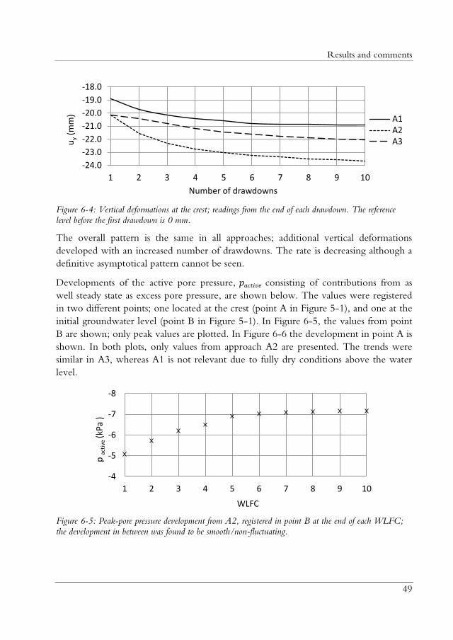
Results and comments
49
Figure 6-4: Vertical deformations at the crest; readings from the end of each drawdown. The reference level before the first drawdown is 0 mm.
The overall pattern is the same in all approaches; additional vertical deformations
developed with an increased number of drawdowns. The rate is decreasing although a
definitive asymptotical pattern cannot be seen.
Developments of the active pore pressure, consisting of contributions from as
well steady state as excess pore pressure, are shown below. The values were registered
in two different points; one located at the crest (point A in Figure 5-1), and one at the
initial groundwater level (point B in Figure 5-1). In Figure 6-5, the values from point
B are shown; only peak values are plotted. In Figure 6-6 the development in point A is
shown. In both plots, only values from approach A2 are presented. The trends were
similar in A3, whereas A1 is not relevant due to fully dry conditions above the water
level.
Figure 6-5: Peak-pore pressure development from A2, registered in point B at the end of each WLFC; the development in between was found to be smooth/non-fluctuating.
-24.0
-23.0
-22.0
-21.0
-20.0
-19.0
-18.0
1 2 3 4 5 6 7 8 9 10
uy
(mm
)
Number of drawdowns
A1A2A3
-8
-7
-6
-5
-4
1 2 3 4 5 6 7 8 9 10
p a
ctiv
e (k
Pa )
WLFC

Impact of water-level variations on slope stability
50
Figure 6-6: Pore-pressure development from A2, registered in point A.
In Figure 6-7 a picture of the flow region—the area where the external water level and
the slope surface intersect—is shown. Total (resultant) flow is represented by arrows.
The picture shows the conditions prevailing after the first WLFC was run, but is
qualitatively characteristic for the endpoints of all WLFC’s.
Figure 6-7: A sample picture of the area where the external water level and the slope intersect, showing the hydraulic conditions prevailing immediately after the first WLFC run in A1. The external water level is located at +22 m whereas the groundwater table within the slope is lower. The flow directions are presented by arrows.
-80.4
-80.3
-80.2
-80.1
-80.0
-79.9
-79.8
-79.7
-79.6
0 1 2 3 4 5 6 7 8 9 10
p a
ctiv
e (k
Pa
)
WLFC

Results and comments
51
In Figure 6-8 - Figure 6-13 flow conditions registered immediately after each WLFC
are presented. Since the readings were taken at the end of each cycle, the external
water level and the groundwater table are almost coinciding, meaning small absolute
magnitudes of the flow values registered. The flow condition for each stage is
presented as the deviation from the average value of the 10 cycles. Maximum total
flow, and horizontal flow directed inwards (in to the slope), is presented
in Figure 6-8 and Figure 6-9, whereas maximum vertical flow (upward, , and
downward, ) is shown in Figure 6-10 and Figure 6-11. All of the maximum
and minimum values are originating from the region being marked in Figure 6-7,
except the values of . The latter ones are registered just below the groundwater
table, approximately 10 m right (inwards) from the slope surface.
Figure 6-8: Maximum total flow; average ~0.1 m/day.
Figure 6-9: Rightward directed horizontal flow; average ~0.08 m/day.
-60%
-30%
0%
30%
60%
90%
1 2 3 4 5 6 7 8 8 10
|qm
ax|(
dev
iati
on
fro
m
aver
age)
WLFC
A1
A2
A3
-100%
-50%
0%
50%
100%
150%
1 2 3 4 5 6 7 8 9 10qx,
rig
ht (
dev
iati
on
fro
m
aver
age)
WLFC
A1
A2
A3
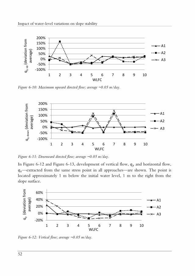
Impact of water-level variations on slope stability
52
Figure 6-10: Maximum upward directed flow; average ~0.05 m/day.
Figure 6-11: Downward directed flow; average ~0.05 m/day.
In Figure 6-12 and Figure 6-13, development of vertical flow, and horizontal flow,
—extracted from the same stress point in all approaches—are shown. The point is
located approximately 1 m below the initial water level, 1 m to the right from the
slope surface.
Figure 6-12: Vertical flow; average ~0.05 m/day.
-100%
-50%
0%
50%
100%
150%
200%
1 2 3 4 5 6 7 8 9 10
qy,
up (
dev
iati
on
fro
m
aver
age)
WLFC
A1
A2
A3
-100%
-50%
0%
50%
100%
150%
200%
1 2 3 4 5 6 7 8 9 10
qy,
do
wn (
dev
iati
on
fro
m
aver
age)
WLFC
A1
A2
A3
-20%
0%
20%
40%
60%
1 2 3 4 5 6 7 8 9 10
qy
(d
evia
tio
n f
rom
av
erag
e)
WLFC
A1
A2
A3
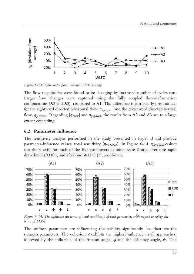
Results and comments
53
Figure 6-13: Horizontal flow; average ~0.05 m/day.
The flow magnitudes were found to be changing by increased number of cycles run.
Larger flow changes were captured using the fully coupled flow-deformation
computations (A2 and A3), compared to A1. The difference is particularly pronounced
for the rightward directed horizontal flow, and the downward directed vertical
flow, . Regarding and the results from A2 and A3 are to a large
extent coinciding.
6.2 Parameter influence
The sensitivity analysis performed in the study presented in Paper B did provide
parameter-influence values; total sensitivity ( ). In Figure 6-14 -values
(on the y-axis) for each of the five parameters at initial state (Init.), after one rapid
drawdown (RDD), and after one WLFC (1), are shown.
(A1) (A2) (A3)
Figure 6-14: The influence (in terms of total sensitivity) of each parameter, with respect to safety (in terms of FOS).
The stiffness parameters are influencing the stability significantly less than are the
strength parameters. The cohesion, exhibits the highest influence in all approaches;
followed by the influence of the friction angle, and the dilatancy angle, . The
-20%
0%
20%
40%
60%
1 2 3 4 5 6 7 8 9 10
qx
(d
evia
tio
n f
rom
av
erag
e)
WLFC
A1
A2
A3
0%
10%
20%
30%
40%
50%
60%
70%
ν c φ ψ E0%
10%
20%
30%
40%
50%
60%
70%
ν c φ ψ E0%
10%
20%
30%
40%
50%
60%
70%
ν c φ ψ E
Init.
RDD
1

Impact of water-level variations on slope stability
54
influence of as well Poisson’s ratio, as of Young’s modulus, is slightly increasing
during further cycling; though remaining below 3% and 2%, respectively. Therefore,
the stiffness parameters are excluded from the presentation of the further sensitivity
development, presented in Figure 6-15 - Figure 6-17.
Figure 6-15: Sensitivity development for cohesion, c. The dotted lines are showing the initial values for each modelling approach (A10, A20, and A30).
Figure 6-16: Sensitivity development for friction angle, . The dotted lines are showing the initial values for each modelling approach (A10, A20, and A30).
50%
52%
54%
56%
58%
60%
1 2 3 4 5 6 7 8 9 10
Sen
siti
vity
(co
hes
ion
)
WLFC
A1
A2
A3
A30
A10
A20
30%
32%
34%
36%
38%
40%
1 2 3 4 5 6 7 8 9 10
Sen
siti
vity
(fr
icti
on
an
gle)
WLFC
A1
A2
A3
A30
A10
A20

Results and comments
55
Figure 6-17. Sensitivity development for dilatancy angle, . The dotted lines are showing the initial values for each modelling approach (A10, A20, and A30).
It is clear that the sensitivity values are depending on the stage at which the safety is
evaluated, i.e. on the numbers of WLFC’s run. For cohesion, the qualitative trend is
the same in all cases; maximum influence at drawdown and then declining with
increased number of WLFC’s. In A1 the sensitivity of cohesion gets lower than the
initial value after 5 WLFC’s; in A2 this occurs at 2 WLFC’s, and in A3 the initial value
is not reached at all during the 10 cycles. For the friction angle, the pattern is
opposite; minimum values at drawdown and then increasing. For this parameter, the
initial values are exceeded in all approaches; in A1 and A2 after 3 WLFC’s, and in A3
after 6 WLFC’s. The total change of the influence of cohesion during 10 cycles, seems
to be similar in all approaches. The increase of the friction-angle influence in A2 seems
to be fading out slower than in A1 and A3. When it comes to the dilatancy angle,
the patterns are more scattered. In all cases the sensitivity values are decreased after the
first drawdown (Figure 6-14), whereas the further development is almost constant.
Though, the absolute magnitudes (and the variations) of the dilatancy-angle influence
are very small, and further conclusions are not reasonably drawn.
5%
6%
7%
8%
9%
1 2 3 4 5 6 7 8 9 10Sen
siti
vity
(d
ilata
ncy
an
gle)
WLFC
A1
A2
A3
A30 A10 A20

Impact of water-level variations on slope stability
56
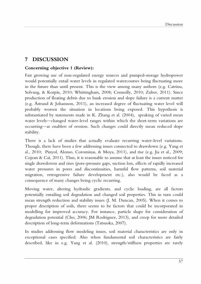
Discussion
57
7 DISCUSSION
Concerning objective 1 (Review):
Fast growing use of non-regulated energy sources and pumped-storage hydropower
would potentially entail water levels in regulated watercourses being fluctuating more
in the future than until present. This is the view among many authors (e.g. Catrinu,
Solvang, & Korpås, 2010; Whittingham, 2008; Connolly, 2010; Zuber, 2011). Since
production of floating debris due to bank erosion and slope failure is a current matter
(e.g. Åstrand & Johansson, 2011), an increased degree of fluctuating water level will
probably worsen the situation in locations being exposed. This hypothesis is
substantiated by statements made in K. Zhang et al. (2004), speaking of varied mean
water levels—changed water-level ranges within which the short-term variations are
occurring—as enablers of erosion. Such changes could directly mean reduced slope
stability.
There is a lack of studies that actually evaluate recurring water-level variations.
Though, there have been a few addressing issues connected to drawdown (e.g. Yang et
al., 2010; Pinyol, Alonso, Corominas, & Moya, 2011), and rise (e.g. Jia et al., 2009;
Cojean & Caï, 2011). Thus, it is reasonable to assume that at least the issues noticed for
single drawdowns and rises (pore-pressure gaps, suction loss, effects of rapidly increased
water pressures in pores and discontinuities, harmful flow patterns, soil material
migration, retrogressive failure development etc.), also would be faced as a
consequence of many changes being cyclic recurring.
Moving water, altering hydraulic gradients, and cyclic loading, are all factors
potentially entailing soil degradation and changed soil properties. This in turn could
mean strength reduction and stability issues (J. M. Duncan, 2005). When it comes to
proper description of soils, there seems to be factors that could be incorporated in
modelling for improved accuracy. For instance, particle shape for consideration of
degradation potential (Cho, 2006; JM Rodriguez, 2013), and creep for more detailed
description of long-term deformations (Tatsuoka, 2007).
In studies addressing flow modeling issues, soil material characteristics are only in
exceptional cases specified. Also when fundamental soil characteristics are fairly
described, like in e.g. Yang et al. (2010), strength/stiffness properties are rarely

Impact of water-level variations on slope stability
58
considered. Therefore, the coupling between soil deformation, pore-pressure
development, and water flow conditions are often overlooked and/or missed.
Given the important and critical connections involving pore pressures, soil strength,
soil-deformation development, (and so on)—stated in Huang & Jia (2009), Galavi
(2010), and Sheng (2011)—it seems to be unreasonable to use simple limit-
equilibrium methods for analysis of slopes subjected to water-level fluctuations.
Concerning objective 2 (Impacts on a slope subjected to water-level
fluctuations—FEM-modelling):
The modelling performed in this study—given the specific conditions of soil
properties, slope geometry, and pattern of water-level changes—showed that the
water-level fluctuations resulted in growing stability and development of vertical
deformations at the slope crest. The stability increase is to assign to the fact that the
groundwater table is dropping (remained at a lower level) for each WLFC. Though,
since rapid changes of pore pressures and flow rates were noticed within the slope,
other upcoming issues could probably occur as well suddenly as in the long term.
The development of the pore-pressure peak values (registered at the initial water level,
point B in Figure 5-1) shows how the pore pressure at the end of each WLFC, slowly
becomes more and more negative. This increase of the negative pore pressure indicates
that the groundwater table is dropping for each cycle, contributing to an increased
stability. This in turn means that equilibrium between groundwater level and external
water level was not reached during the ten cycles. If such fluctuations are taking place
for a long time, negative pore pressures could falsely remain high. If then the
fluctuation stops, the water levels would go back to equilibrium, and the extra shear
strength would be lost. This phenomenon of suction loss would potentially get
consequences similar to those noticed in situations of wetting-induced strength loss
presented in e.g. (Jia et al. (2009). The pore-pressure development registered both in
point A and B did show asymptotic patterns. Also the deformation increase was fading
out. This might indicate that the slope was approaching a state where only elastic
strains were developed at further WLFC’s.
In situations where internal erosion is taking place, the soil is definitely getting changed
properties. Since e.g. hydraulic conductivity has been shown to significantly affect the
stability of reservoir slopes consisting of sand and silt (Liao et al., 2005), material
changes would be preferably considered in long-term modelling.
Despite the fact that the absolute magnitudes of differences identified in this study were
small—FOS-values, pore pressures, flows etc.—these do nonetheless demonstrate
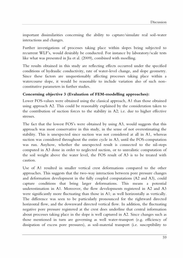
Discussion
59
important dissimilarities concerning the ability to capture/simulate real soil-water
interactions and changes.
Further investigations of processes taking place within slopes being subjected to
recurrent WLF’s, would desirably be conducted. For instance by laboratory/scale tests
like what was presented in Jia et al. (2009), combined with moelling.
The results obtained in this study are reflecting effects occurred under the specified
conditions of hydraulic conductivity, rate of water-level change, and slope geometry.
Since these factors are unquestionably affecting processes taking place within a
watercourse slope, it would be reasonable to include variation also of such non-
constitutive parameters in further studies.
Concerning objective 3 (Evaluation of FEM-modelling approaches):
Lower FOS-values were obtained using the classical approach, A1 than those obtained
using approach A2. This could be reasonably explained by the consideration taken to
the contribution of suction forces to the stability in A2; i.e. due to higher effective
stresses.
The fact that the lowest FOS’s were obtained by using A3, would suggests that this
approach was most conservative in this study, in the sense of not overestimating the
stability. This is unexpected since suction was not considered at all in A1, whereas
suction was considered throughout the entire cycle in A3, until the FOS-computation
was run. Anyhow, whether the unexpected result is connected to the nil-steps
computed in A3 done in order to neglected suction, or to unrealistic computation of
the soil weight above the water level, the FOS result of A3 is to be treated with
caution.
Use of A1 resulted in smaller vertical crest deformations compared to the other
approaches. This suggests that the two-way interaction between pore pressure changes
and deformation development in the fully coupled computations (A2 and A3), could
capture conditions that bring larger deformations. This means a potential
underestimation in A1. Moreover, the flow developments registered in A2 and A3
were significantly more fluctuating than those in A1; as well horizontally as vertically.
The difference was seen to be particularly pronounced for the rightward directed
horizontal flow, and the downward directed vertical flow. In addition, the fluctuating
negative pore pressure registered at the crest does underline that central information
about processes taking place in the slope is well captured in A2. Since changes such as
those mentioned in turn are governing as well water-transport (e.g. efficiency of
dissipation of excess pore pressures), as soil-material transport (i.e. susceptibility to

Impact of water-level variations on slope stability
60
internal erosion to be initiated and/or continued), modelling approaches not being
fully coupled are probably not suitable for analysis of processes being governed by
fluctuating flows, altering hydraulic gradients, unloading/reloading etc. In that sense—
in agreement with what was concluded in Sheng et al. (2013)—there seems to be
situations where approaches considering unsaturated soil behavior is not necessarily less
conservative than are classical ones.
Since hydraulic models do rely on empirical soil-specific parameters, there are potential
uncertainties connected to the level of accuracy at which these have been quantified.
Still, this uncertainty is to be related to the extra information possibly obtained at
consideration of specific features of unsaturated soils.
Concerning objective 4 (Parameter-sensitivity analysis):
The parameter-sensitivity analysis results obtained using A1 seems to be quantitatively
more comparable to those obtained using A3 than to those obtained using A2. This
suggests that consideration of suction at stability computation (only true in A2), does
directly affect the parameter influence on the results. However, major differences were
not found. Since the sensitivity was computed with respect to FOS determined by
using the strength reduction technique, the low and insignificantly changing sensitivity
values of the stiffness parameters were expected. The non-constant sensitivity values of
the dilatancy angle, might indicate that the occurrences of plastic strains are somewhat
different in the different stages.
It might be useful to consider parameter influence for evaluation of the accuracy
needed for definition of model input data; as well absolute magnitudes, as the
development patterns. Moreover, when making up modelling/design strategies, parameter changes (e.g. by time or by external changes taking place), could be valuably
included.
Conclusions
61
8 CONCLUSIONS
8.1 General
Concerning objective 1 (Review):
It seems to be consensus among researchers and experts that the fast growing use
of non-regulated energy sources and pumped-storage hydropower, will entail
water levels in regulated watercourses being fluctuating more in the future than
until present.
Water-level changes have been shown to significantly influence slope stability;
failure due to suction loss, effects of rapidly increased water pressures (as well in
pores as in discontinuities), potentially harmful flow patterns, internal erosion,
and retrogressive failure development.
Moving water, altering hydraulic gradients, soil-material transport, and cyclic
external loading, are all factors potentially entailing soil degradation, property
changes, strength reduction, and stability issues.
Given the important and critical connections involving pore pressures, soil
strength, and soil-deformation development, it is not reasonable to use simple
limit-equilibrium methods for analysis of slopes subjected to water-level
fluctuations.
Concerning objective 2 (Impacts on a slope subjected to water-level
fluctuations—FEM-modelling):
Water-level fluctuations resulted in growing stability, development of vertical
deformations at the slope crest, and rapidly fluctuating flows (as well horizontal
as vertical) within the slope.
Even though the stability might remain unchanged or even increase due to
fluctuations of an external water level, rapid changes of pore pressures and flow
within the slope, could mean upcoming issues as well suddenly as in the long
term.
Concerning objective 3 (Evaluation of FEM-modelling approaches):
Modelling assuming strictly saturated or dry conditions resulted in—restricted to
slope stability in terms of safety factors—higher conservatism compared to

Impact of water-level variations on slope stability
62
modelling considering also the behavior of unsaturated soil and fully hydro-
mechanical coupling.
Modelling considering the behavior of unsaturated soil and fully hydro-
mechanical coupling, but with suction neglected at stability computation, was
shown to give safety factors even lower than did classical modelling. Whether
this was due to the saturation-suction relation in the hydraulic model used, or
due to the nil-steps run prior to the FOS-computations, the importance of
being careful when complex situations are designed, is however underlined.
Advanced modelling seems to allow for rapid changes of pore pressures and
flow to be more realistically described than do classical modelling. Since such
changes in turn are governing as well water-transport (i.e. the efficiency of
dissipation of excess pore pressures), as soil-material transport (i.e. susceptibility
to internal erosion to be initiated and/or continued), simplified modelling
approaches are not suitable for analysis of processes being governed by
fluctuating flows, altering hydraulic gradients, unloading/reloading etc.
Concerning objective 4 (Parameter-sensitivity analysis):
The influence of the parameters on the slope stability was found to be changing
as a result of WLFC’s taking place.
For evaluation of the accuracy needed for modelling-input data, it might be
useful to consider parameter influence; as well total values, as the development
patterns. Moreover, when making up modelling/design strategies, inclusion of
parameter changes (e.g. by time or by external changes taking place), could be
valuable.
8.2 To be further considered
In order to properly simulate groundwater flow—capturing also effects besides critical
development of pore-pressures, flow patterns, and subsequent stability changes—consideration should be taken to:
Use of a more advanced constitutive soil model (e.g. the Hardening soil model
PLAXIS, 2012) would potentially reduce inaccuracy coming from e.g.
improper description of plastic deformations and stiffness changes. The water-
level fluctuation effects would also be investigated using models based on the
Basic Barcelona Model (Alonso, Gens, & Josa, 1990).
Incorporate varied hydraulic conductivity in sensitivity analyses.
Conclusions
63
Vary frequencies and rates of water-level changes, slope geometries etc. (in
previous studies simple approaches are used focusing on one or a few cycles), for
further investigation.
Design a modelling approach for application to long-term effects of WLF’s on
potential debris production along regulated watercourses.
Indirect consider internal-erosion in embankments (dams and/or watercourse
banks), by incorporating parameter changes in the modelling.
Further investigate processes taking place within slopes being subjected to
recurrent WLF’s, e.g. by laboratory/scale tests like what was presented in Jia et
al. (2009) .

Impact of water-level variations on slope stability
64
References
65
REFERENCES
Alonso, E. E., Gens, A., & Josa, A. (1990). A constitutive model for partially saturated soils.
Géotechnique, vol. 40, no. 3, pp. 405–430.
Axelsson, K. (1998). Introduktion till Jordmekaniken jämte jordmaterialläran. Luleå:
Division of Mining and Geotechnical Engineering, Luleå University of Technology.
Bakhtyar, R., Barry, D. A., Li, L., Jeng, D. S., & Yeganeh-Bakhtiary, A. (2009). Modeling
sediment transport in the swash zone: A review. Ocean Engineering, vol. 36, no. 9-10, pp.
767–783.
Bardi, U. (2009). Peak oil: The four stages of a new idea. Energy, vol. 34, no. 3, pp. 323–
326.
Biot, M. A. (1941). General Theory of Three-Dimensional Consolidation. Journal of Applied
Physics, vol. 12, no. 2, pp. 155.
Bolton, M. D. (1986). The strength and dilatancy of sands. Geotechnique, , no. I.
Briaud, J. (2013). Geotechnical Engineering: Unsaturated and Saturated Soils. John Wiley
& Sons, Inc.
Bruun, P. (1988). The Bruun rule of erosion by sea-level rise: a discussion on large-scale
two-and three-dimensional usages. Journal of Coastal Research, vol. 4, no. 4, pp. 627–
648.
Burland, J. B., & Jennings, J. E. B. (1962). Limitations to the Use of Effective Stresses in
Partly Saturated Soils. Géotechnique, vol. 12, no. 2, pp. 125–144.
Catrinu, M. D., Solvang, E., & Korpås, M. (2010). Pe spectives on hyd opowe ’ s ole to
balance non-regulated renewable power production in Northern and Western Europe. In
HYDRO 2011, okt 17 - okt 20. Prague.
Chappell, J., Eliot, I., Bradshaw, M., & Lonsdale, E. (1979). Experimental control of beach
face dynamics by watertable pumping. Engineering Geology, vol. 14, no. 1, pp. 29–41.
Cho, G.-C., Dodds, J., & Santamarina, J. C. (2006). Particle Shape Effects on Packing
Density, Stiffness, and Strength: Natural and Crushed Sands. Journal of Geotechnical and
Geoenvironmental Engineering, vol. 132, no. 5, pp. 591–602.
Cojean, R., & Caï, Y. J. (2011). Analysis and modeling of slope stability in the Three-Gorges
Dam reservoir (China) — The case of Huangtupo landslide. Journal of Mountain Science,
vol. 8, no. 2, pp. 166–175.
Connolly, D. (2010). A Review of Energy Storage Technologies - For the integration of
fluctuating renewable energy. PhD thesis, University of Limerick., Limerick, Ireland.
Craig, R. F. (2004). C aig’s soil mechanics. CRC Press.
Darby, S. E., Rinaldi, M., & Dapporto, S. (2007). Coupled simulations of fluvial erosion and
mass wasting for cohesive river banks. Journal of Geophysical Research, vol. 112, no. F3,
pp. F03022.

Impact of water-level variations on slope stability
66
Di Benedetto, H., Tatsuoka, F., & Ishihara, M. (2002). Time-dependent shear deformation
characteristics of sand and their constitutive modelling. Soils and foundations, vol. 42, no.
2, pp. 1–22.
Duncan, J. M. (1996). State of the Art: Limit Equilibrium and Finite-Element Analysis of
Slopes. Journal of Geotechnical Engineering, vol. 122, no. 7, pp. 577–596.
Duncan, J. M., & Wright, S. G. (1980). The accuracy of equilibrium methods of slope
stability analysis. Engineering Geology, vol. 16, no. 1-2, pp. 5–17.
Duncan, J. M., & Wright, S. G. (2005). Soil Strength and Slope Stability. Hoboken, New
Jersey: John Wiley & Sons, Inc.
Duncan, J. R. (1964). The effects of water table and tide cycle on swash-backwash sediment
distribution and beach profile development. Marine Geology, vol. 2, no. 3, pp. 186–197.
Emery, K., & Foster, J. (1948). Water tables in marine beaches. Journal of Marine Research,
vol. 7, pp. 644–654.
Fox, G. A., Wilson, G. V, Simon, A., Langendoen, E. J., Akay, O., & Fuchs, J. W. (2007).
Measuring streambank erosion due to ground water seepage: correlation to bank pore
water pressure, precipitation and stream stage. Earth Surface Processes and Landforms,
vol. 32, no. 10, pp. 1558–1573.
Fredlund, D. G. (2006). Unsaturated Soil Mechanics in Engineering Practice. Journal of
Geotechnical and Geoenvironmental Engineering, vol. 132, no. 3, pp. 286–321.
Fredlund, D. G., & Morgenstern, N. (1977). Stress state variables for unsaturated soils.
Journal of Geotechnical and Geoenvironmental Engineering, vol. 103, no. GT5, pp. 447–
466.
Fredlund, D. G., Xing, A., & Huang, S. (1994). Predicting the permeability function for
unsaturated soils using the soil-water characteristic curve. Canadian Geotechnical
Journal, vol. 31, no. 4, pp. 533–546.
Galavi, V. (2010). Internal Report - Groundwater flow, fully coupled flow deformation and
undrained analyses in PLAXIS 2D and 3D.
Grant, U. (1948). Influence of the water table on beach aggradation and degradation.
Journal of Marine Research, vol. 7, pp. 650–655.
Guimaraes, M. (2002). Crushed stone fines and ion removal from clay slurries - fundamental
studies. Georgia Institute of Technology.
Gärdenäs, A. I., Šimůnek, J., Jarvis, N., & van Genuchten, M. T. (2006). Two-dimensional
modelling of preferential water flow and pesticide transport from a tile-drained field.
Journal of Hydrology, vol. 329, no. 3-4, pp. 647–660.
Hansbo, S. (1975). Jordmateriallära. Uppsala: Almqvist & Wiksell.
Huang, M., & Jia, C.-Q. (2009). Strength reduction FEM in stability analysis of soil slopes
subjected to transient unsaturated seepage. Computers and Geotechnics, vol. 36, no. 1-2,
pp. 93–101.
Hupp, C. (1992). Riparian vegetation recovery patterns following stream channelization: a
geomorphic perspective. Ecology, vol. 73, no. 4, pp. 1209–1226.
References
67
Jia, G. W., Zhan, T. L. T., Chen, Y. M., & Fredlund, D. G. (2009). Performance of a large-
scale slope model subjected to rising and lowering water levels. Engineering Geology,
vol. 106, no. 1-2, pp. 92–103.
Johansson, J. M. A., & Vall, J. (2011). Friktionsjords kornform. pure.ltu.se. Luleå Univeristy
of Technology, Luleå.
Kaczmarek, J., & Leśniewska, D. (2011). Modelling Events Occurring in the Core of a Flood
Bank and Initiated by Changes in the Groundwater Level, Including the Effect of Seepage.
Technical Sciences, vol. 14, no. 14.
Krahn, J. (2003). The 2001 R.M. Hardy Lecture: The limits of limit equilibrium analyses.
Canadian Geotechnical Journal, vol. 40, no. 3, pp. 643–660.
Krumbein, W. C. (1941). Measurement and Geological Significance of Shape and Roundness
of Sedimentary Particles. SEPM Journal of Sedimentary Research, vol. Vol. 11, no. 2, pp.
64–72.
Kuhn, M. R., & Mitchell, J. K. (1993). New Perspectives on Soil Creep. Journal of
Geotechnical Engineering, vol. 119, no. 3, pp. 507–524.
Kuwano, R., & Jardine, R. (2002). On measuring creep behaviour in granular materials
through triaxial testing. Canadian Geotechnical Journal, vol. 1074, pp. 1061–1074.
Lade, P. V., & Liu, C.-T. (1998). Experimental Study of Drained Creep Behavior of Sand.
Journal of Engineering Mechanics, vol. 124, no. 8, pp. 912–920.
Lafleur, J. (1984). Filter testing of broadly graded cohesionless tills. Canadian Geotechnical
Journal, vol. 21, no. 4, pp. 634–643.
Lane, P. A., & Griffiths, D. V. (1999). Slope stability analysis by finite elements.
Géotechnique, vol. 49, no. 3, pp. 387–403.
Lane, P. A., & Griffiths, D. V. (2000). Assessment of Stability of Slopes under Drawdown
Conditions. Journal of Geotechnical and Geoenvironmental Engineering, vol. 126, no. 5,
pp. 443–450.
Li, L., Barry, D. A., Parlange, J.-Y., & Pattiaratchi, C. B. (1997). Beach water table
fluctuations due to wave run-up: Capillarity effects. Water Resources Research, vol. 33,
no. 5, pp. 935–945.
Li, L., Barry, D. A., & Pattiaratchi, C. B. (1997). Numerical modelling of tide-induced beach
water table fluctuations. Coastal Engineering, vol. 30, no. 1-2, pp. 105–123.
Liao, H., Ying, J., Gao, S., & Sheng, Q. (2005). Numerical Analysis on Slope Stability under
Variations of Reservoir Water Level. In Landslides (pp. 305–311). Springer Berlin
Heidelberg.
Lim, T., Rahardjo, H., Chang, M., & Fredlund, D. G. (1996). Effect of rainfall on matric
suctions in a residual soil slope. Canadian Geotechnical Journal, vol. 33, no. 4, pp. 618–
628.
Liu, C., Li, F., Ma, L.-P., & Cheng, H.-M. (2010). Advanced materials for energy storage.
Advanced materials, vol. 22, no. 8, pp. E28–E62.
López-Acosta, N. P., Fuente de la, H. A., & Auvinet, G. (2013). Safety of a protection levee
under rapid drawdown conditions. Coupled analysis of transient seepage and stability. In

Impact of water-level variations on slope stability
68
Proceedings of the 18th International Conference on Soil Mechanics and Geotechnical
Engineering, Paris 2013 (pp. 3305–3308).
Mill, O., Dahlbäck, A., Wörman, S., Knutsson, S., Johansson, F., Andreasson, P., …
Glavatskih, S. (2010). Analysis and Development of Hydro Power Research - Synthesis
within Swedish Hydro Power Centre. Stockholm.
Minarski, R. (2008). Assessment of the potential amount of floating debris in Lule river.
Luleå University of Technology.
Mitchell, J., & Soga, K. (2005). Fundamentals of soil behavior. John Wiley & Sons, Inc.
Morgenstern, N. (1963). Stability Charts for Earth Slopes During Rapid Drawdown.
Géotechnique, vol. 13, no. 2, pp. 121–131.
Murayama, S., Michihiro, K., & Sakagami, T. (1984). Creep characteristics of sand. Soils
and foundations, vol. 24, no. 5.
Nielsen, P. (1990). Tidal dynamics of the water table in beaches. Water Resources Research,
vol. 26, no. 9, pp. 2127–2134.
Parlange, J., Stagnitti, F., Starr, J., & Braddock, R. (1984). Free-surface flow in porous
media and periodic solution of the shallow-flow approximation. Journal of Hydrology,
vol. 70, no. 1-4, pp. 251–263.
Peng, F.-L., Tan, K., & Tan, Y. (2012). Simulating the Viscous Behavior of Sandy Ground by
FEM. In GeoCongress 2012 (pp. 2167–2176). Reston, VA: American Society of Civil
Engineers.
Pereira, J.-M., Coussy, O., Alonso, E. E., Vaunat, J., & Olivella, S. (2010). Is the degree of
sat ation a good candidate fo Bishop’s pa amete ? In A. Gens (Ed.), Alonso, E.E.,
Gens, A. (eds.) Unsaturated Soils—Proceedings of 5th International Conference on
Unsaturated Soils (pp. 913–919). Geophysics, Barcelona, Spain, September 2010: CRC
Press.
Petterson, K. E. (1955). The Early History of Circular Sliding Surfaces. Géotechnique, vol. 5,
no. 4, pp. 275–296.
Pinyol, N. M., Alonso, E. E., Corominas, J., & Moya, J. (2011). Canelles landslide:
modelling rapid drawdown and fast potential sliding. Landslides, vol. 9, no. 1, pp. 33–51.
PLAXIS. (2012). PLAXIS 2D 2012. Delft, Netherlands.: Available at: http://www.plaxis.nl/.
Pugh, D. T. (1987). Tides, Surges and Mean Sea-Level. Marine and Petroleum Geology (Vol.
5, p. 301). John Wiley & Sons, Inc.
R. Grove, J., Croke, J., & Thompson, C. (2013). Quantifying different riverbank erosion
processes during an extreme flood event. Earth Surface Processes and Landforms, vol.
1406, no. February, pp. n/a–n/a.
Ramalho, R. S., Quartau, R., Trenhaile, A. S., Mitchell, N. C., Woodroffe, C. D., & Ávila, S.
P. (2013). Coastal evolution on volcanic oceanic islands: A complex interplay between
volcanism, erosion, sedimentation, sea-level change and biogenic production. Earth-
Science Reviews, vol. 127, pp. 140–170.
Raubenheimer, B., Guza, R. T., & Elgar, S. (1999). Tidal water table fluctuations in a sandy
ocean beach. Water Resources Research, vol. 35, no. 8, pp. 2313–2320.
REN21. (2013). Renewables 2013: Global Status Report.

References
69
Rodriguez, J., Edeskär, T., & Knutsson, S. (2013). Particle Shape Quantities and
Measurement Techniques–A Review. Electronical Journal of Geotechnical Engineering,
vol. 18, pp. 169–198.
Rodriguez, J., Johansson, J., & Edeskär, T. (2012). Particle shape determination by two-
dimensional image analysis in geotechnical engineering. In Nordic Geotechnical Meeting,
NGM 2012, 16, 9-12 May, 2012. (pp. 207–218).
Rognlien, L. M. (2012). Pumped storage hydropower development in Øvre Otra, Norway.
Norwegian University of Science and Technology.
Rowe, P. W. (1962). The Stress-Dilatancy Relation for Static Equilibrium of an Assembly of
Particles in Contact. Proceedings of the Royal Society A: Mathematical, Physical and
Engineering Sciences, vol. 269, no. 1339, pp. 500–527.
Santamarina, J. C., & Cho, G. C. (2004). Soil behavio : he ole of pa ticle shape, pp. 1–
14.
Schweiger, H. F., & Peschl, G. M. (2005). Reliability analysis in geotechnics with the
random set finite element method. Computers and Geotechnics, vol. 32, no. 6, pp. 422–
435.
Shen, Y., Zhu, D., & Yao, H. (2010). Critical slip field of slope in process of reservoir water
level fluctuations. Rock and Soil Mechanics, vol. 31, no. S2, pp. 179–183.
Sheng, D. (2011). Review of fundamental principles in modelling unsaturated soil behaviour.
Computers and Geotechnics, vol. 38, no. 6, pp. 757–776.
Sheng, D., Zhang, S., & Yu, Z. (2013). Unanswered questions in unsaturated soil mechanics.
Science China Technological Sciences, vol. 56, no. 5, pp. 1257–1272.
Singhroy, V. (1995). Sar integrated techniques for geohazard assessment. Advances in Space
Research, vol. 15, no. 11, pp. 67–78.
Smith-Konter, B., & Pappalardo, R. T. (2008). Tidally driven stress accumulation and shear
fail e of ncelad s’s tige st ipes. Icarus, vol. 198, no. 2, pp. 435–451.
Solvang, E., Harby, A., & Killingtveit, Å. (2012). Increasing balance power capacity in
Norwegian hydroelectric power stations.
Sun, D., Sun, W., & Xiang, L. (2010). Effect of degree of saturation on mechanical
behaviour of unsaturated soils and its elastoplastic simulation. Computers and
Geotechnics, vol. 37, no. 5, pp. 678–688.
Swedenergy. (2008). RIDAS.
Svenska Kraftnät. (2008). Storskalig utbyggnad av vindkraft (Vol. 1).
Tatsuoka, F. (2000). Some new aspects of time effects on the stress-strain behaviour of stiff
geomaterials, Keynote Lecture. The Geotechnics of Hard Soils-Soft Rocks, Proc. of
Second Int. Conf. on Hard Soils and Soft Rocks, Napoli, 1998, vol. 2, pp. 1285–1371.
Tatsuoka, F. (2007). Inelastic deformation characteristics of geomaterial. In Soil Stress-
Strain Behavior: Measurement, Modeling and Analysis (Vol. 146, pp. 1–108). Springer
Netherlands.
Terzaghi, K., Peck, R., & Mesri, G. (1996). Soil mechanics in engineering practice (p. 1565).
Impact of water-level variations on slope stability
70
Thomas, A., Eldho, T. I., & Rastogi, a. K. (2013). A comparative study of point collocation
based MeshFree and finite element methods for groundwater flow simulation. ISH Journal
of Hydraulic Engineering, , no. January 2014, pp. 1–10.
Tohari, A., Nishigaki, M., & Komatsu, M. (2007). Laboratory Rainfall-Induced Slope
Failure with Moisture Content Measurement. Journal of Geotechnical and
Geoenvironmental Engineering, vol. 133, no. 5, pp. 575–587.
Tsai, T.-L., & Yang, J.-C. (2006). Modeling of rainfall-triggered shallow landslide.
Environmental Geology, vol. 50, no. 4, pp. 525–534.
U.S. EPA. (1999). TRIM, Total Risk Integrated Methodology, TRIM FATE Technical Support
Document, Volume I: Description of Module.
U.S. EPA. (2001). Risk Assessment Guidance for Superfund (RAGS) Volume III - Part A:
Process for Conducting Probabilistic Risk Assessment (2001) - Appendix A (Vol. 3, pp. 1–
37).
Wadell, H. (1932). Volume, Shape, and Roundness of Rock Particles. The Journal of
Geology, vol. 40, no. 5, pp. 443–451.
Van Genuchten, M. T. (1980). A Closed-form Equation for Predicting the Hydraulic
Conductivity of Unsaturated Soils. Soil Science Society of America Journal, vol. 44, no. 5,
pp. 892–898.
Ward, W. H. (1945). The Stability of Natural Slopes. The Geographical Journal, vol. 105, no.
5/6, pp. 170.
Whittingham, M. (2008). Materials challenges facing electrical energy storage. Mrs
Bulletin, vol. 33, no. 04, pp. 411–419.
Yang, H., Rahardjo, H., & Xiao, D. (2010). Rapid Drawdown of Water Table in Layered Soil
Column. In Geoenvironmental engineering and geotechnics: progress in modeling and
applications (pp. 202–209). Shanghai, China: American Society of Civil Engineers
(ASCE).
Yu, H. S., Salgado, R., Sloan, S. W., & Kim, J. M. (1998). Limit Analysis versus Limit
Equilibrium for Slope Stability. Journal of Geotechnical and Geoenvironmental
Engineering, vol. 124, no. 1, pp. 1–11.
Zhan, T., Zhang, W., & Chen, Y. (2006). Influence of reservoir level change on slope
stability of a silty soil bank. In The Fourth International Conference on Unsaturated Soils,
ASCE, April 2–4 (pp. 463–472).
Zhang, C. (2013). Non-Tidal Water Level Variability in Lianyungang Coastal Area.
Advanced Materials Research, vol. 610, pp. 2705–2708.
Zhang, K., Douglas, B. C., & Leatherman, S. P. (2004). Global Warming and Coastal
Erosion. Climatic Change, vol. 64, no. 1-2, pp. 41–58.
Zheng, H., Sun, G., & Liu, D. (2009). A practical procedure for searching critical slip
surfaces of slopes based on the strength reduction technique. Computers and Geotechnics,
vol. 36, no. 1-2, pp. 1–5.
Zuber, M. (2011). Renaissance for Pumped Storage in Europe. RenewableEnergyWorld.com
(publ. augusti 20, 2011). Retrieved October 02, 2012, from
References
71
http://www.renewableenergyworld.com/rea/news/article/2011/08/renaissance-for-
pumped-storage-in-europe
Åstrand, S., & Johansson, N. (2011). Drivgods vid extrema tillfällen, Elforsk, Rapport 11:32.
Stockholm.


Paper A
Effects of External Water-Level Fluctuations on Slope
Stability
J. M. Johansson and T. Edeskär
Electronic Journal of Geotechnical Engineering vol. 19, no. K, pp. 2437–2463, 2014.

Jens M. A. Johansson
Tommy Edeskär
ABSTRACT
KEYWORDS:
- 2437 -

Vol. 19 [2014], Bund. K 2438
INTRODUCTION
Vol. 19 [2014], Bund. K 2439
WATER LEVEL VARIATION – MODES AND SOURCES
General
Long-term natural variations
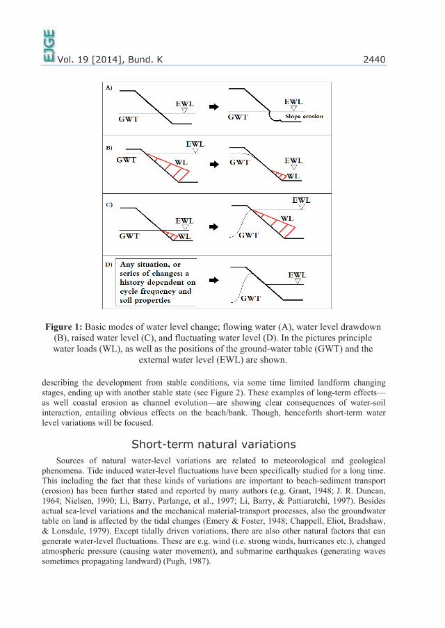
Vol. 19 [2014], Bund. K 2440
Short-term natural variations
Figure 1:
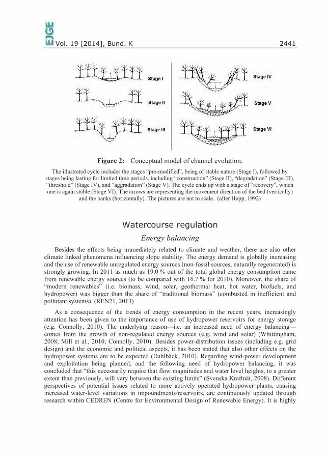
Vol. 19 [2014], Bund. K 2441
Watercourse regulation
Figure 2:

Vol. 19 [2014], Bund. K 2442
WATER-LEVEL VARIATION AND SLOPE STABILITY – EFFECTS AND CONSIDERATIONS
Analysis of slope stability

Vol. 19 [2014], Bund. K 2443
= ´= = + ( ) tan ( )
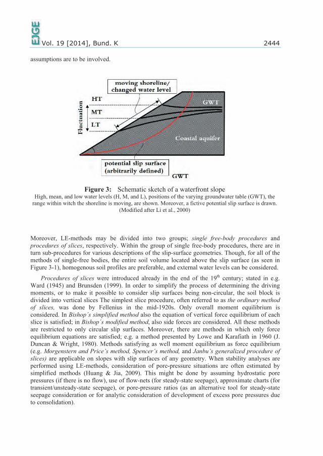
Vol. 19 [2014], Bund. K 2444
Figure 3:
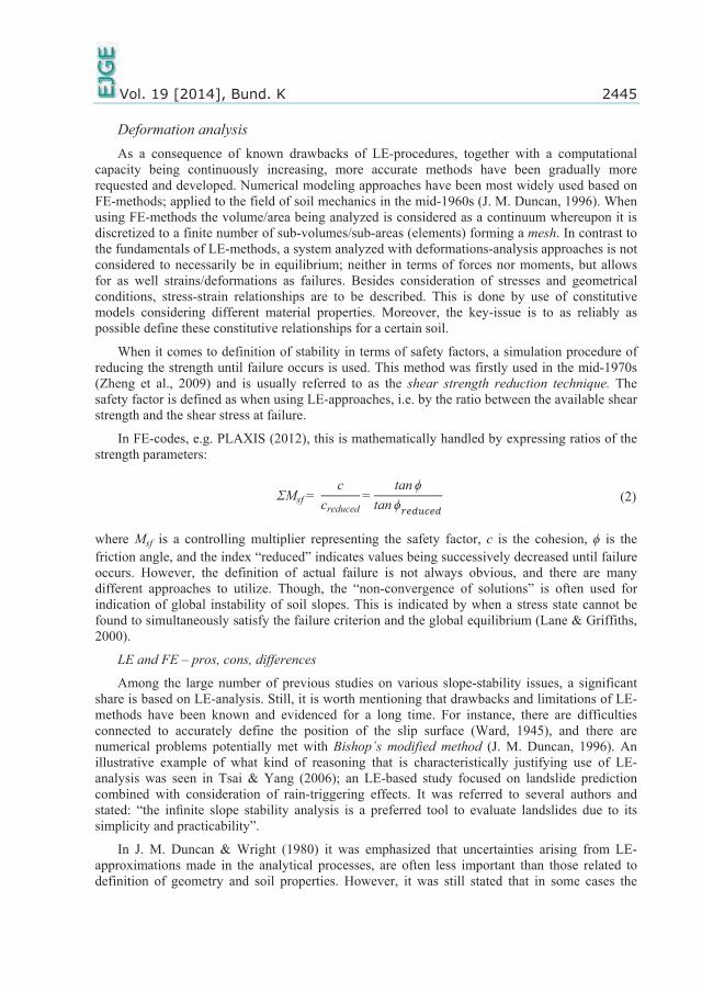
Vol. 19 [2014], Bund. K 2445
Vol. 19 [2014], Bund. K 2446
Water-level drawdown

Vol. 19 [2014], Bund. K 2447
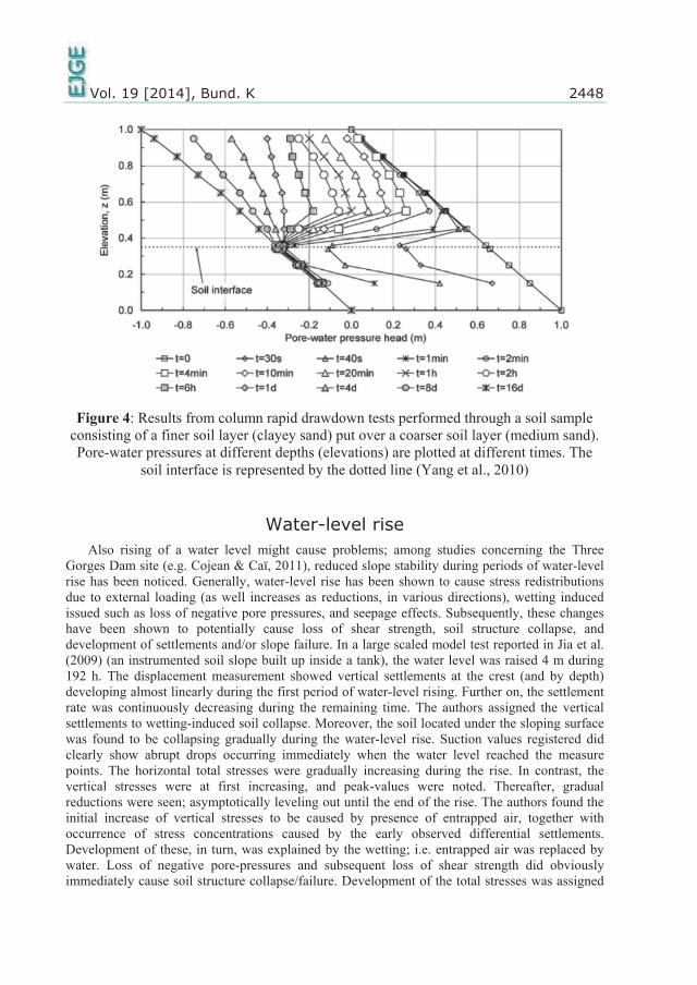
Vol. 19 [2014], Bund. K 2448
Water-level rise
Figure 4

Vol. 19 [2014], Bund. K 2449
Water-level fluctuation: drawdown-rise combinations
Hydrological modeling
Vol. 19 [2014], Bund. K 2450

Vol. 19 [2014], Bund. K 2451
Seepage – internal erosion
Vol. 19 [2014], Bund. K 2452
Vol. 19 [2014], Bund. K 2453
Vol. 19 [2014], Bund. K 2454
CONCLUDING DISCUSSION

Vol. 19 [2014], Bund. K 2455

Vol. 19 [2014], Bund. K 2456
ASPECTS TO BE FURTHER CONSIDERED
Vol. 19 [2014], Bund. K 2457
ACKNOWLEDGEMENTS
REFERENCES

Vol. 19 [2014], Bund. K 2458

Vol. 19 [2014], Bund. K 2459
Vol. 19 [2014], Bund. K 2460

Vol. 19 [2014], Bund. K 2461
Vol. 19 [2014], Bund. K 2462

Vol. 19 [2014], Bund. K 2463


Paper B
Modelling approaches considering impacts of water-level
fluctuations on slope stability
J. M. Johansson and T. Edeskär
To be submitted

1
Modelling approaches considering impacts of water-level fluctuations
on slope stability
Jens M.A. Johansson1; Tommy Edeskär
2
Abstract
Waterfront slopes are affected by water-level fluctuations originating from as well natural sources (e.g. tides and wind
waves), as non-natural sources such as watercourse regulation involving daily or hourly recurring water-level
fluctuations. Potentially instable slopes in populated areas means risks for as well property as human lives. In this
study, three different approaches used for hydro-mechanical coupling in FEM-modelling of slope stability, have been
evaluated. A fictive slope consisting of a till-like soil material has been modeled to be exposed to a series of water-
level fluctuation cycles (WLFC’s). Modelling based on assuming fully saturated conditions, and with computations of
flow and deformations separately run, has been put against two approaches being more sophisticated, with
unsaturated-soil behavior considered and with computations of pore-pressures and deformations simultaneously run.
Development of stability, vertical displacements, pore pressures, flow, and model-parameter influence, has been
investigated for an increased number of WLFC’s. It was found that more advanced approaches did allow for capturing
larger variations of flow and pore pressures. Classical modelling resulted in smaller vertical displacements, and
smoother development of pore-pressure and flow. Flow patterns, changes of soil density (linked to volume changes
governed by suction fluctuations), and changes of hydraulic conductivity, are all factors governing as well water-
transport (e.g. efficiency of dissipation of excess pore pressures) as soil-material transport (i.e. susceptibility to
internal erosion to be initiated and/or continued). Therefore, the results shown underline potential strengths of
sophisticated modelling. Parameter influence was shown to change during water-level cycling.
Key words: Hydro-mechanical coupling; Water-level fluctuations; Slope stability; Unsaturated soil; FEM-analysis;
Parameter influence
1 Introduction
When it comes to recurring water-level fluctuations in watercourses and reservoirs, effects of hydrological
changes on slope stability are often overlooked. There is a predominance of studies focused on
bioenvironmental issues [1]. The activity of watercourse regulation for water storage, enabling irrigation,
freshwater provision, and hydropower production, often means occurrence of water-level fluctuations (e.g.
[2–4]). The growing use of non-regulated energy sources (e.g. wind and solar) [5, 2, 6, 7]—bringing
significant emphasis put on wind-power development and exploitation—entails a need of energy balancing
by water storage in reservoirs. According to [8], this will necessarily require that flow magnitudes and
water level heights, to a greater extent than until present, will vary in the future. It is highly expected to get
increased variations of the reservoir water levels; hour to hour, day to day and/or seasonally [9, 2, 4].
The process of rapid drawdown is described and investigated by many authors e.g. [10–13]. Also water-
level rise might cause problems. In studies concerning the Three Gorges Dam site (e.g. [14]), slope stability
reductions registered during periods of water-level rise, have been reported. Rise of water levels has been
shown to cause stress redistributions due to external loading, wetting induced loss of negative pore
pressures, and seepage effects. Subsequently, these changes have been shown to potentially cause loss of
shear strength, soil structure collapse, and development of settlements and/or slope failure [15]. It has been
emphasized that a delayed change of pore water pressure inside a slope—relative to the external water
level—may result in significant movements of water within the slope; creating seepage forces being
adversely affecting the stability [15].
Despite well-known limitations of limit-equilibrium methods (LEM) (e.g. [11, 16]), these are well
established and widely used. For capturing important relations between pore pressure, soil strength, and
1 Department of Civil, Environmental and Natural Resources Engineering, Luleå University of Technology 2 Department of Civil, Environmental and Natural Resources Engineering, Luleå University of Technology
2
soil-deformation development, the use of finite-element methods (FEM) have been more and more spread.
Long-term perspectives are important for consideration of altering hydraulic gradients, stress-strain
changes, and development of influenced waterfront zones. Still, reliable relationships between soil
deformation, pore-pressure development, and unsteady water-flow conditions are often deliberately
overlooked or incidentally missed [1]. Though, improved accessibility of high computer capacity allows for
more and more advanced analyses to be performed. In addition, optimized designs and constructions are
increasingly demanded and less conservative design approaches are therefore often desired. This is not at
least linked to economic and environmental aspects. One non-conservative view in slope-stability analysis
regards consideration of negative pore pressures in unsaturated soils. Taking into account negative pore
pressures is generally associated with counting on extra contributions to the shear strength of the soil,
resulting in extra slope stability. The well-known and widely used Terzaghi´s equation of effective-stress
( – u) is simply based upon the difference between the total stress, and the pore pressure, u. The
equation implies that there are only two possible soil conditions; (1) presence of pore pressure coming from
fully water filled pores, and (2) no pore pressure. The validity of this expression is widely accepted in
saturated soil mechanics, but has since a long time been found to not be applicable for partly saturated
conditions, e.g. [17]. The possibility to control the mechanical response of unsaturated soils by considering
two stress-state variables—(1) net stress, i.e. the difference between the total stress and the pore-air
pressure, and (2) suction, i.e. the difference between the pore-air pressure and the pore-water pressure—was
firstly demonstrated by [18]. Though, the earliest effective-stress equation for consideration of a varying
degree of saturation and suction was presented by Bishop in the end of the 1950th. For description of the
amount of water being present in unsaturated soils, soil-water characteristic curves (SWCC) are important.
The degree of saturation, (among other alternatively use quantities) appears to most closely control the
behavior of unsaturated soil [19]. For proper consideration of the behavior of unsaturated soils, fully
coupled hydro-mechanical computations are needed (e.g. [20–22]).
Among studies with hydro-mechanical approaches applied, many are addressing sediment-loading
problems; sources, changed river shapes caused by sedimentation etc. (e.g. [23–25]). Consequently, the
slope-stability part is often either absent or considered by using LEM-approaches (e.g. [26–28]). There are
a few studies addressing effects of large-scale reservoir water-level fluctuations on slope stability; e.g. [29]
where saturated-unsaturated seepage analysis was combined with LEM-stability analysis, and [30] where
evaluation of the approach of analyzing stability using critical slip fields. The complexity of how factors
such as drawdown rate, permeability, and slope height actually do influence the stability of a slope
subjected to drawdown, was discussed in [20].
In [31] it was emphasized the misconception concerning that analysis approaches considering principles
of unsaturated soil mechanics are always less conservative than are classical ones. It was stated that the
overall subject is at its early stage, that there are numerous areas in which practical application of the
principles of unsaturated soil mechanics are central, and that as well experimental as theoretical advances
are expected.
The present study is aimed to evaluate results from three approaches of hydro-mechanical coupling in
FEM-modelling of slope stability; (1) semi-coupled modelling, (2) fully coupled modelling, and (3) fully
coupled modelling, but with negative pore pressures neglected in stability computations. In (1) flow
computations were run prior to those of deformations, and Terzaghi’s effective-stress definition was used.
In (2) pore-pressure development and deformations were simultaneously computed, utilizing Bishop’s
effective-stress definition, considering also the behavior of unsaturated soils. Approach (3) is similar to (2),
but with suction effects in stability computation neglected. A fictive waterfront bank slope consisting of a
well-graded postglacial till, typical for Swedish conditions, was modeled to be subjected to a series of
water-level-fluctuation cycles (WLFC’s). Development of stability (in terms of factors of safety, FOS),
vertical displacements, pore pressures, flow, and model-parameter influence, was investigated for an
increased number of WLFC’s. The modelling was performed by use of the software PLAXIS 2D 2012 [32],
allowing for consideration of transient flow and performance of coupled hydro-mechanical computations.
Moreover, parameter-influence analysis was performed with respect to FOS’s calculated using the strength
reduction technique; i.e. the parameter-influence development with an increased number of WLFC’s was
investigated.

3
2 Methodology
2.1 Model design and preparations
2.1.1 Geometry, materials, and definition of changes
The model geometry was defined aimed to represent one half of a watercourse cross section. The slope
height was set to 30 m, and the slope inclination to 1:2 (26.6°) (Figure 2-1); both measures considered to be
representative for a watercourse slope consisting of a well-graded till, typical for Swedish conditions
(properties presented in Table 1). 15-noded triangular elements were used.
The vertical model boundaries were set to be horizontally fixed and free to move vertically, whereas the
bottom boundary was completely fixed. The left vertical boundary was assumed to have properties of a
symmetry line, and the model bottom to represent a material being dense and stiff relative to the soil above.
Therefore, as well the left vertical hydraulic boundary as the horizontal bottom, were defined as closed
(impermeable). The right vertical boundary was defined to be assigned pore pressures by the head,
simulating allowed in/out flow. Data-collection points were placed where interesting changes would be
expected; at the crest, down along the slope surface, and along a vertical line below the crest.
The initial water-level position was set to +22.0 m (with the level of the watercourse bottom at ± 0 m), the
level-change magnitude to 5.0 m (linearly lowered and raised), and the rate to 1.0 m/day. In [33] situations
with daily magnitudes of water-level variations in pumped-storage hydropower (PSH) in the order of 10 m
were discussed, and in [20] a rate of 1 m/day was used in rapid drawdown analysis. Since this study is
comparative, the rate used was chosen in order to create a stability reduction at drawdown, avoid failure,
and still be within a relevant and representative range. The water-level changes were run continuously; i.e.
without allowing pore pressures to even out.
Figure 2-1: Model geometry. Dimensions, initial water level (WLinitial), and the pre-defined data-collection
points—one at the crest (A) and one at the level +22 m (B)—are shown in the figure.

4
Table 1: Model input data used.
Unit Value Comments
General Drainage type - - Drained
Unsaturated weight kN/m3 19.00 Typical value
Saturated weight kN/m3 21.00 Typical value
Soil description
Young´s modulus kN/m2 40 000 2)
Poisson´s ratio - 0.30 2)
Cohesion kN/m2 8 Low, non-zero
Friction angle ° 36 Typical value
Dilatancy angle ° 3 Meeting the recommendation
Hydraulic description
Model
van Genuchten
Data set - - - Defined in order to be representative 1)
Permeability, x m/day 0.05 Found to be representative (e.g. Lafleur, 1984)
Permeability, y m/day 0.05 Found to be representative (e.g. Lafleur, 1984)
Saturated degr. of sat. - 1.0
Residual degr. of sat. - 0.026 1)
- - 1.169 Parameter linked to water extraction 1)
- - 2.490 Parameter linked to air entry 1)
- - 0 Parameter linked to pore connectivity 1)
1)
The data set was manually defined by using the parameters listed. The values of the parameters , , , ,
and were chosen based on examples in [22], comments in [35], and the pre-defined data set Hypres available in
PLAXIS 2D 2012 [36]. 2)
Within ranges presented in [37]; Young´s modulus for a loose glacial till (10-150 MPa), and for a medium/compact
sand (30-50 MPa), at - .
NOTE: Since the result evaluation is comparative, the values of the parameters chosen are not critical.
2.2 Modelling strategy
2.2.1 Approaches evaluated
Approach 1 (A1):
The computations were performed using Terzaghi's definition of stress, i.e. [ ], where is the
normal stress, is the effective normal stress, and is the pore pressure consisting of steady-state pore
pressure (from the phreatic level or groundwater flow computations) and excess pore pressure (coming
from undrained behavior or consolidation; i.e. temporal pore-pressure changes governed by the WLF’s and
captured by consideration of transient water flow). In this semi-coupled approach, flow computations were
run prior to the deformation computations. Pore pressures from the flow computations were, for each time
step, used in the deformation computation for the corresponding time step. The consolidation computations
were based on excess pore pressures.
Approach 2 (A2): For the fully coupled approach Bishop’s effective-stress equation was used. The consolidation
computations were based on the Biot’s theory of consolidation [38]; i.e. using total pore pressures with no
distinction made between steady state and excess pore pressures.
Approach 3 (A3):
Computations run like in A2, but with stability computations run without consideration of negative pore
pressures.
5
2.2.2 Behavior of unsaturated soil
For the fully coupled approaches (A2 and A3), Bishop’s effective-stress equation was used, allowing for
capturing the unsaturated soil behavior:
( ) (2.1)
where is the pore-air pressure, the pore-water pressure, and the experimentally determined matric-
suction coefficient being related to the degree of saturation, . The experimental evidences of are sparse
[22], and the role of the parameter has been generally questioned [19]. In PLAXIS 2D 2012 the matric-
suction coefficient is substituted with the effective degree of saturation, , defined as:
( ) ( ) (2.2)
where is the degree of saturation and the indices max and min denote maximum and minimum values.
Moreover, in this study the air-pore pressure is assumed to be negligibly low, whereupon the effective
stress is simply expressed as:
(2.3)
The effective degree of saturation is used also for definition of actual soil unit weight, :
( ) (2.4)
where the indices denote unsaturated and saturated conditions.
2.2.3 Models used
The constitutive behavior of the soil was described by Mohr-Coulomb’s elastic-perfectly plastic model.
This model was chosen for three reasons; (1) it is well-established and widely used by engineers, (2) as
soon as the stability analysis is started (performed using the strength reduction technique), any model
defined with the same strength parameters would behave like the Mohr-Coulomb model (i.e. stress
dependent stiffness is excluded), (3) the study is comparative whereupon differences between the modelling
approaches evaluated are focused rather than the accuracy of the soil description. For other
permissions/claims, models like e.g. the Hardening soil model [32] (allowing for description of more
realistic elastic-plastic behaviors), or the Basic Barcelona Model [39] (specifically developed for
description of the stress-strain behavior in unsaturated soils), could have been used. The soil was defined by
the variables listed in Table 1. The elastic behavior is described by the parameters Young´s modulus, and
Poisson´s ratio, . The full three-dimensional yield criterion consists of six yield functions; two functions in
each plane of stress pairs. Each yield function depends on one stress pair (one combination of the principal
effective stresses), the friction angle, and the cohesion, . These are defining the ultimate state up to
which the strains are elastic; for stress conditions entailing that the yield function is reached, the strain
response becomes perfectly plastic. For these conditions the strain magnitudes are determined using flow
rules based on plastic potential functions. These are—similar to the yield functions—depending on the
stress state, but are consisting of three plastic parameters; in addition to the friction angle, and the
cohesion, , also the dilatancy angle, . This parameter is used for description of additional resistance
against shearing, originating from dilatant behavior.
For description of hydraulic behavior in the soil, van Genuchten’s model [40] was used. The important
role of the hydraulic model is to properly define the degree of saturation, as a function of suction pore-
pressure head, . This relation, often presented in soil-water characteristic curves (SWCC), is expressed:
( ) ( )[ ( | |)
] (2.5)

6
where is the residual degree of saturation, is the saturated degree of saturation, is an empirical
parameter describing air entry, and is an empirical parameter related to the water extraction from the
soil. The relative permeability, ( ) is expressed as:
( ) [ (
)
]
(2.6)
where is an empirical parameter. The relative permeability is in the flow computation reducing the
permeability according to ( ⁄ ) where is the saturated permeability.
2.2.4 Factor of safety
The strength reduction (or phi/c-reduction) technique is based on FOS’s defined as the ratio between the
available shear strength and the shear stress at failure. In PLAXIS 2D 2012 this is mathematically handled
by expressing ratios of the strength parameters:
(2.7)
where is a controlling multiplier representing the safety factor; c is the cohesion; is the friction
angle; and the index reduced indicates values being successively decreased until failure occurs. For
indication of global instability of soil slopes, the non-convergence of solutions is often used. This is
indicated by the condition when a stress state at which the failure criterion and the global equilibrium can
be simultaneously satisfied, is not found [10].
2.2.5 Parameter-sensitivity analysis
The parameter influence was investigated with respect to changed FOS. For each parameter, a maximum
and a minimum value were defined spanning a representative interval within which the reference value for
each parameter (presented in Table 1) was located. The theories used are based on the ratio of the
percentage change of the result, and the percentage change of input (creating the output change); explained
in e.g. [41]. The sensitivity ratio [42] is expressed as:
( ( ) ( )
( )) (
)⁄ (2.8)
where the output values are functions, of the input values, for which no index represents the reference
input values and the index U,L represents the changed ones; upper/lower. In order to increase the
robustness [32] of the analysis, the sensitivity ratio was weighted by a normalized variability measure. This
was done using a sensitivity score, , defined as the ratio of the range itself and the variable mean value
[42]:
(
) (2.9)
where and define the range limits, and is the mean (reference) value. The total sensitivity
was then calculated as:
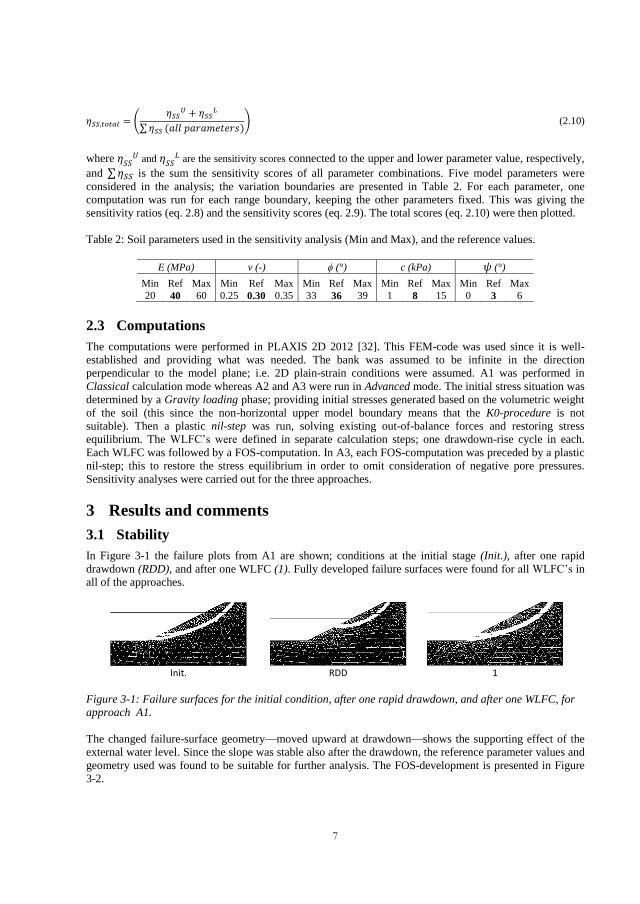
7
(
∑ ( )) (2.10)
where and
are the sensitivity scores connected to the upper and lower parameter value, respectively,
and ∑ is the sum the sensitivity scores of all parameter combinations. Five model parameters were
considered in the analysis; the variation boundaries are presented in Table 2. For each parameter, one
computation was run for each range boundary, keeping the other parameters fixed. This was giving the
sensitivity ratios (eq. 2.8) and the sensitivity scores (eq. 2.9). The total scores (eq. 2.10) were then plotted.
Table 2: Soil parameters used in the sensitivity analysis (Min and Max), and the reference values.
E (MPa) v (-) (°) c (kPa) (°)
Min Ref Max Min Ref Max Min Ref Max Min Ref Max Min Ref Max
20 40 60 0.25 0.30 0.35 33 36 39 1 8 15 0 3 6
2.3 Computations
The computations were performed in PLAXIS 2D 2012 [32]. This FEM-code was used since it is well-
established and providing what was needed. The bank was assumed to be infinite in the direction
perpendicular to the model plane; i.e. 2D plain-strain conditions were assumed. A1 was performed in
Classical calculation mode whereas A2 and A3 were run in Advanced mode. The initial stress situation was
determined by a Gravity loading phase; providing initial stresses generated based on the volumetric weight
of the soil (this since the non-horizontal upper model boundary means that the K0-procedure is not
suitable). Then a plastic nil-step was run, solving existing out-of-balance forces and restoring stress
equilibrium. The WLFC’s were defined in separate calculation steps; one drawdown-rise cycle in each.
Each WLFC was followed by a FOS-computation. In A3, each FOS-computation was preceded by a plastic
nil-step; this to restore the stress equilibrium in order to omit consideration of negative pore pressures.
Sensitivity analyses were carried out for the three approaches.
3 Results and comments
3.1 Stability
In Figure 3-1 the failure plots from A1 are shown; conditions at the initial stage (Init.), after one rapid
drawdown (RDD), and after one WLFC (1). Fully developed failure surfaces were found for all WLFC’s in
all of the approaches.
Init. RDD 1
Figure 3-1: Failure surfaces for the initial condition, after one rapid drawdown, and after one WLFC, for
approach A1.
The changed failure-surface geometry—moved upward at drawdown—shows the supporting effect of the
external water level. Since the slope was stable also after the drawdown, the reference parameter values and
geometry used was found to be suitable for further analysis. The FOS-development is presented in Figure
3-2.

8
Figure 3-2: FOS-values for initial conditions (Init.), after one rapid drawdown (RDD), and after one
WLFC (1) (picture to the left); and development by additional WLFC’s (picture to the right).
For all approaches—with the initial conditions as references—the FOS-values were significantly decreasing
due to the rapid drawdown (about 17% for A1, and 16% for A2 and A3), slightly increasing due to the first
WLFC (3% for A1 and 2% for A2 and A3), and ending up exhibiting further increased values after 10
WLFC’s (a total increase of 6 % for A1, and 5% for A2 and A3). The results show that the stability growth
continues during the entire period studied.
Lower FOS-values were obtained using the approach assuming saturated conditions below the water-
level, dry conditions above, and taking into account neither pore-pressure changes due to deformations, nor
suction (A1), than using fully coupled flow-deformation computations, considering also suction forces
(A2). This is reasonably explained by the consideration taken to the contribution of suction forces to the
stability. The lowest FOS-values were obtained in A3; i.e. fully coupled flow-deformation computations,
but with the negative pore pressures not considered in the stability analysis. These FOS-values were found
to be even lower than those obtained in A1; this although suction was neglected also in A1.
3.2 Deformations, pore pressures and flow
In Figure 3-3, vertical deformations developed at the crest (point A, see Figure 2-1) are presented. The
values were registered in the middle of each WLFC, i.e. at the end of each drawdown.
Figure 3-3: Vertical deformations at the crest; readings from the end of each drawdown. The reference
level before the first drawdown is 0 mm.
The overall pattern is the same in all approaches; additional vertical deformations are developed with an
increased number of drawdowns. The rate is decreasing although a definitive asymptotical pattern cannot
be seen. Utilization of A1 seems to give less deformations developed compared to both A2 and A3. This
was found to be true at all depths vertically below point A (see Figure 2-1).
The development of the active pore pressure, (consisting of contributions from as well steady
state as excess pore pressure) measured in A2, is shown in Figure 3-4. The developments were registered in
two different points; one located at the crest (point A in Figure 2-1), and one at the initial groundwater level
(point B in Figure 2-1).
1.30
1.40
1.50
1.60
1.70
1.80
Init. RDD 1
FOS A1
A2
A3 1.65
1.70
1.75
1.80
1.85
1 2 3 4 5 6 7 8 9 10
FOS
WLFC
A1A2A3
-24.0-23.0-22.0-21.0-20.0-19.0-18.0
1 2 3 4 5 6 7 8 9 10
uy
(mm
)
Number of drawdowns
A1
A2
A3
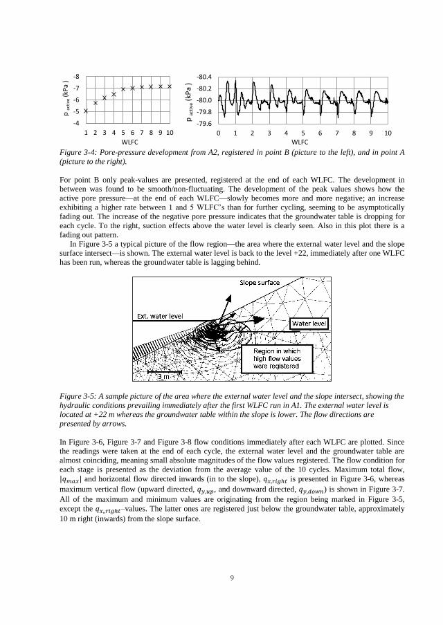
9
Figure 3-4: Pore-pressure development from A2, registered in point B (picture to the left), and in point A
(picture to the right).
For point B only peak-values are presented, registered at the end of each WLFC. The development in
between was found to be smooth/non-fluctuating. The development of the peak values shows how the
active pore pressure—at the end of each WLFC—slowly becomes more and more negative; an increase
exhibiting a higher rate between 1 and 5 WLFC’s than for further cycling, seeming to be asymptotically
fading out. The increase of the negative pore pressure indicates that the groundwater table is dropping for
each cycle. To the right, suction effects above the water level is clearly seen. Also in this plot there is a
fading out pattern.
In Figure 3-5 a typical picture of the flow region—the area where the external water level and the slope
surface intersect—is shown. The external water level is back to the level +22, immediately after one WLFC
has been run, whereas the groundwater table is lagging behind.
Figure 3-5: A sample picture of the area where the external water level and the slope intersect, showing the
hydraulic conditions prevailing immediately after the first WLFC run in A1. The external water level is
located at +22 m whereas the groundwater table within the slope is lower. The flow directions are
presented by arrows.
In Figure 3-6, Figure 3-7 and Figure 3-8 flow conditions immediately after each WLFC are plotted. Since
the readings were taken at the end of each cycle, the external water level and the groundwater table are
almost coinciding, meaning small absolute magnitudes of the flow values registered. The flow condition for
each stage is presented as the deviation from the average value of the 10 cycles. Maximum total flow,
and horizontal flow directed inwards (in to the slope), is presented in Figure 3-6, whereas
maximum vertical flow (upward directed, , and downward directed, ) is shown in Figure 3-7.
All of the maximum and minimum values are originating from the region being marked in Figure 3-5,
except the –values. The latter ones are registered just below the groundwater table, approximately
10 m right (inwards) from the slope surface.
-8
-7
-6
-5
-4
1 2 3 4 5 6 7 8 9 10
p a
ctiv
e (
kPa
)
WLFC
-80.4
-80.2
-80.0
-79.8
-79.6
0 1 2 3 4 5 6 7 8 9 10
p a
ctiv
e (k
Pa
)
WLFC
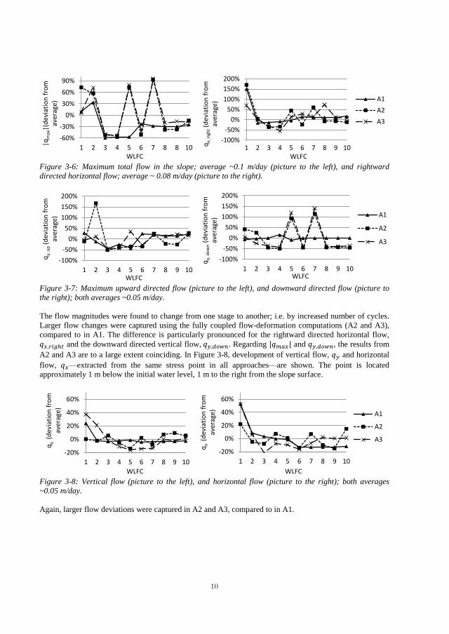
10
Figure 3-6: Maximum total flow in the slope; average ~0.1 m/day (picture to the left), and rightward
directed horizontal flow; average ~ 0.08 m/day (picture to the right).
Figure 3-7: Maximum upward directed flow (picture to the left), and downward directed flow (picture to
the right); both averages ~0.05 m/day.
The flow magnitudes were found to change from one stage to another; i.e. by increased number of cycles.
Larger flow changes were captured using the fully coupled flow-deformation computations (A2 and A3),
compared to in A1. The difference is particularly pronounced for the rightward directed horizontal flow,
and the downward directed vertical flow, . Regarding and , the results from
A2 and A3 are to a large extent coinciding. In Figure 3-8, development of vertical flow, and horizontal
flow, —extracted from the same stress point in all approaches—are shown. The point is located
approximately 1 m below the initial water level, 1 m to the right from the slope surface.
Figure 3-8: Vertical flow (picture to the left), and horizontal flow (picture to the right); both averages
~0.05 m/day.
Again, larger flow deviations were captured in A2 and A3, compared to in A1.
-60%
-30%
0%
30%
60%
90%
1 2 3 4 5 6 7 8 8 10
|qm
ax|(
dev
iati
on
fro
m
aver
age)
WLFC
-100%
-50%
0%
50%
100%
150%
200%
1 2 3 4 5 6 7 8 9 10qx,
rig
ht (
dev
iati
on
fro
m
aver
age)
WLFC
A1
A2
A3
-100%
-50%
0%
50%
100%
150%
200%
1 2 3 4 5 6 7 8 9 10
qy,
up (
dev
iati
on
fro
m
aver
age)
WLFC
-100%
-50%
0%
50%
100%
150%
200%
1 2 3 4 5 6 7 8 9 10
qy,
do
wn (
dev
iati
on
fro
m
aver
age)
WLFC
A1
A2
A3
-20%
0%
20%
40%
60%
1 2 3 4 5 6 7 8 9 10
qy (
dev
iati
on
fro
m
aver
age)
WLFC
-20%
0%
20%
40%
60%
1 2 3 4 5 6 7 8 9 10
qx (
dev
iati
on
fro
m
aver
age)
WLFC
A1
A2
A3
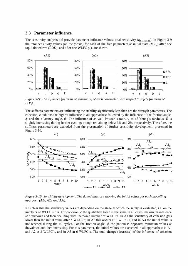
11
3.3 Parameter influence
The sensitivity analysis did provide parameter-influence values; total sensitivity ( ). In Figure 3-9
the total sensitivity values (on the y-axis) for each of the five parameters at initial state (Init.), after one
rapid drawdown (RDD), and after one WLFC (1), are shown.
(A1) (A2) (A3)
Figure 3-9: The influence (in terms of sensitivity) of each parameter, with respect to safety (in terms of
FOS).
The stiffness parameters are influencing the stability significantly less than are the strength parameters. The
cohesion, exhibits the highest influence in all approaches; followed by the influence of the friction angle,
and the dilatancy angle, . The influence of as well Poisson’s ratio, as of Young’s modulus, is
slightly increasing during further cycling; though remaining below 3% and 2%, respectively. Therefore, the
stiffness parameters are excluded from the presentation of further sensitivity development, presented in
Figure 3-10. ( ) ( ) ( )
Figure 3-10: Sensitivity development. The dotted lines are showing the initial values for each modelling
approach (A10, A20, and A30).
It is clear that the sensitivity values are depending on the stage at which the safety is evaluated, i.e. on the
numbers of WLFC’s run. For cohesion, the qualitative trend is the same in all cases; maximum influence
at drawdown and then declining with increased number of WLFC’s. In A1 the sensitivity of cohesion gets
lower than the initial value after 5 WLFC’s; in A2 this occurs at 2 WLFC’s, and in A3 the initial value is
not reached during the 10 cycles. For the friction angle, the pattern is opposite; minimum values at
drawdown and then increasing. For this parameter, the initial values are exceeded in all approaches; in A1
and A2 at 3 WLFC’s, and in A3 at 6 WLFC’s. The total change (decrease) of the influence of cohesion
0%
20%
40%
60%
80%
ν c φ ψ E
0%
20%
40%
60%
80%
ν c φ ψ E0%
20%
40%
60%
80%
ν c φ ψ E
Init.
RDD
1
50%
52%
54%
56%
58%
60%
1 2 3 4 5 6 7 8 9 10
Sen
siti
vity
WLFC
A30
A10
A20
30%
32%
34%
36%
38%
40%
1 2 3 4 5 6 7 8 9 10WLFC
A1 A2 A3
A30
A10
A20
5%
6%
7%
8%
9%
1 2 3 4 5 6 7 8 9 10
WLFC
A30 A10
A20
12
(during 10 cycles) seems to be similar in all approaches, whereas the increase of the friction-angle influence
in A2 seems to be fading out slower than in A1 and A3. When it comes to the dilatancy angle, the
patterns are more scattered. In all cases the sensitivity values are decreased after the first drawdown, whilst
the further development is almost constant. Though, the absolute magnitudes (and the variations) of the
dilatancy-angle influence are very small, and further conclusions are not reasonably drawn.
4 Discussion
Despite the fact that the absolute magnitudes of differences identified in this study were small—FOS-
values, pore pressures, flows etc.—these do nonetheless demonstrate important dissimilarities concerning
the ability to capture/simulate real soil-water interactions and changes. The results of FOS-development
show that the stability growth continues during the entire period studied; though not smoothly. The stability
increase is to assign to the fact that the groundwater table is dropping (remained at a lower level) for each
WLFC; this was also confirmed by the pore-pressure developments discussed. Lower FOS-values were
obtained using the classical approach, A1 than those obtained using approach A2. This could be reasonably
explained by the consideration taken to the contribution of suction forces to the stability in A2. The fact that
the lowest FOS’s were obtained by using A3, would suggests that this approach is most conservative in this
study, in the sense of not overestimating the stability. This is unexpected since suction was not considered
at all in A1, whereas suction was considered throughout the entire cycle in A3, until the FOS-computation
was run. Anyhow, whether the unexpected result is connected to the nil-steps computed in A3 done in order
to neglected suction, or to unrealistic computation of the soil weight above the water level, the FOS result
of A3 is to be treated with caution.
Use of A1 resulted in smaller vertical crest deformations compared to the other approaches. This
suggests that the two-way interaction between pore pressure changes and deformation development in the
fully coupled computations (A2 and A3), could capture conditions that bring larger deformations. This
means a potential underestimation in A1. Moreover, the flow developments registered in A2 and A3 were
significantly more fluctuating than those in A1; as well horizontally as vertically. The difference was seen
to be particularly pronounced for the rightward directed horizontal flow, and the downward directed
vertical flow. In agreement with what was stated in [31], also the outcomes from the present study show
that there seems to be situations where computations taking into account unsaturated soil behavior, is not
necessarily less conservative than are classical ones.
The parameter-sensitivity analysis results obtained using A1 seems to be quantitatively more
comparable to those obtained using A3 than to those using A2. This suggests that consideration of suction
at stability computation (only true in A2), does directly affect the parameter influence on the results.
However, major differences were not found. Since the sensitivity was computed with respect to FOS
determined by using the strength reduction technique, the low and insignificantly changing sensitivity
values of the stiffness parameters were expected. The non-constant sensitivity values of the dilatancy angle,
might indicate that the occurrences of plastic strains are somewhat different in the different stages. Though,
the influence is significantly lower than for friction angle and cohesion, and also less changing.
It might be useful to consider parameter influence for evaluation of the accuracy needed for definition of
model input data; as well absolute magnitudes, as the development patterns. Moreover, when making up
modelling/design strategies, parameter changes (e.g. by time or by external changes taking place), could be
valuably included.
The results obtained in this study are reflecting effects occurred under the specified conditions of
hydraulic conductivity, rate of water-level change, and slope geometry. Since these factors are
unquestionably affect processes taking place within a watercourse slope, it would be reasonable to include
variation also of such non-constitutive parameters in further studies.
Since fully coupled flow-soil deformation modelling to a higher degree describes real soil-water
interaction, results from semi-coupled approaches (like A1) are probably not optimal for analysis of
processes being governed by fluctuating flows, altering hydraulic gradients, unloading/reloading etc. Since
hydraulic models do partly rely on empirical soil-specific parameters there are potential uncertainties
connected to the level of accuracy of these. Still, this uncertainty is to be related to the extra information

13
possibly obtained at consideration of specific features of unsaturated soils. Flow patterns, changes of
denseness, and non-constant values of the hydraulic conductivity, are all factors being valuable for proper
modelling. Not at least since such changes in turn are governing as well water-transport (i.e. the efficiency
of dissipation of excess pore pressures), as soil-material transport (i.e. susceptibility to internal erosion to
be initiated and/or continued).
5 Concluding remarks
The soil structure seems to become more stable due to the first WLFC, and the stability growth
continues during the entire period studied. This for all approaches.
Modelling assuming strictly saturated or dry conditions (classical, like in A1) resulted in—restricted to
slope stability in terms of safety factors—higher conservatism compared to modelling considering also
the behavior of unsaturated soil and fully hydro-mechanical coupling (advanced, like in A2).
Modelling considering the behavior of unsaturated soil and fully hydro-mechanical coupling, but with
suction neglected at stability computation (A3) resulted in lower safety factors even compared to
classical modelling (A1). This might be explained by errors due to the saturation-suction relation in the
hydraulic model used, or to the nil-step computations run in order to get the negative pore pressure
neglected.
Advanced modelling seems to allow for rapid changes of pore pressures and flow to be more
realistically captured compared to classical modelling. Such changes in turn are governing as well
water-transport (i.e. the efficiency of dissipation of excess pore pressures), as soil-material transport
(i.e. susceptibility to internal erosion to be initiated and/or continued).
The influence of the parameters were changing as a result of WLFC’s taking place; decreased influence
of cohesion, increased influence of the friction angle, scattered patterns of the influence of the
dilatancy angle.
5.1 To be further considered
In order to capture effects of water-level variation frequencies, rates, slope geometries etc., on slope
stability, investigations should be performed using advanced modelling approaches, and considering real
long-term perspectives. Use of a more advanced constitutive soil model (e.g. the Hardening soil model
[32]) would potentially reduce inaccuracy coming from e.g. improper description of plastic deformations
and stiffness changes. The water-level fluctuation effects would also be investigated using models based on
the Basic Barcelona Model [39]. Parameter influence would be preferably considered when evaluating the
accuracy needed for modelling-input data, as well as when making up modelling/design strategies.
Investigations of processes taking place within slopes being subjected to recurrent WLF’s, would desirably
be conducted. For instance by laboratory/scale tests combined with modelling.
6 Acknowledgements
The research has been supported by the Swedish Hydropower Centre, SVC; established by the Swedish
Energy Agency, Elforsk and Svenska Kraftnät together with Luleå University of Technology, The Royal
Institute of Technology, Chalmers University of Technology and Uppsala University. Participating
agencies, companies and industry associations are: Alstom Hydro Sweden, Andritz Hydro,
Energimyndigheten, E.ON Vattenkraft Sverige, Falu Energi och Vatten, Fortum Generation, Holmen
Energi, Jämtkraft, Jönköping Energi, Karlstads Energi, Mälarenergi, Norconsult, Pöyry SwedPower,
Skellefteå Kraft, Sollefteåforsens, Statkraft Sverige, SveMin, Svenska Kraftnät, Sweco Infrastructure,
Sweco Energuide, Umeå Energi, Vattenfall Vattenkraft, VG Power, WSP and ÅF.
14
7 References
[1] J. M. A. Johansson and T. Edeskär, “Effects of External Water-Level Fluctuations on Slope Stability,” Electron. J. Geotech. Eng., vol. 19, no. K, pp. 2437–2463, 2014.
[2] O. Mill, A. Dahlbäck, S. Wörman, S. Knutsson, F. Johansson, P. Andreasson, J. Yang, U. Lundin, J.-O. Aidanpää, H. Nilsson, M. Cervantes, and S. Glavatskih, “Analysis and Development of Hydro Power Research - Synthesis within Swedish Hydro Power Centre,” Stockholm, 2010.
[3] N. Dahlbäck, “Utvecklingsbehov inom reglerkraftsområdet ur ett vattenkraftperspektiv,” Stockholm, 2010. [4] E. Solvang, A. Harby, and Å. Killingtveit, “Increasing balance power capacity in Norwegian hydroelectric power
stations,” 2012. [5] M. Whittingham, “Materials challenges facing electrical energy storage,” Mrs Bull., vol. 33, no. 04, pp. 411–419,
Jan. 2008. [6] D. Connolly, “A Review of Energy Storage Technologies - For the integration of fluctuating renewable energy,”
PhD thesis, University of Limerick., Limerick, Ireland, 2010. [7] REN21, “Renewables 2013: Global Status Report,” 2013. [8] Svenska Kraftnät, “Storskalig utbyggnad av vindkraft,” 2008. [9] Svenska Energimyndigheten, “Vattenkraften och energisystemet-ER 2008:24,” Eskilstuna, Sweden, 2008. [10] P. A. Lane and D. V. Griffiths, “Assessment of Stability of Slopes under Drawdown Conditions,” J. Geotech.
Geoenvironmental Eng., vol. 126, no. 5, pp. 443–450, May 2000. [11] J. M. Duncan and S. G. Wright, Soil Strength and Slope Stability. Hoboken, New Jersey: John Wiley & Sons, Inc.,
2005. [12] H. Yang, H. Rahardjo, and D. Xiao, “Rapid Drawdown of Water Table in Layered Soil Column,” in
Geoenvironmental engineering and geotechnics: progress in modeling and applications, 2010, pp. 202–209. [13] N. M. Pinyol, E. E. Alonso, J. Corominas, and J. Moya, “Canelles landslide: modelling rapid drawdown and fast
potential sliding,” Landslides, vol. 9, no. 1, pp. 33–51, May 2011. [14] R. Cojean and Y. J. Caï, “Analysis and modeling of slope stability in the Three-Gorges Dam reservoir (China) —
The case of Huangtupo landslide,” J. Mt. Sci., vol. 8, no. 2, pp. 166–175, Mar. 2011. [15] G. W. Jia, T. L. T. Zhan, Y. M. Chen, and D. G. Fredlund, “Performance of a large-scale slope model subjected to
rising and lowering water levels,” Eng. Geol., vol. 106, no. 1–2, pp. 92–103, May 2009. [16] J. Krahn, “The 2001 R.M. Hardy Lecture: The limits of limit equilibrium analyses,” Can. Geotech. J., vol. 40, no. 3,
pp. 643–660, Jun. 2003. [17] J. B. Burland and J. E. B. Jennings, “Limitations to the Use of Effective Stresses in Partly Saturated Soils,”
Géotechnique, vol. 12, no. 2, pp. 125–144, Jan. 1962. [18] D. G. Fredlund and N. Morgenstern, “Stress state variables for unsaturated soils,” J. Geotech. Geoenvironmental Eng.,
vol. 103, no. GT5, pp. 447–466, Jul. 1977. [19] D. G. Fredlund, “Unsaturated Soil Mechanics in Engineering Practice,” J. Geotech. Geoenvironmental Eng., vol. 132,
no. 3, pp. 286–321, Mar. 2006. [20] M. M. Berilgen, “Investigation of stability of slopes under drawdown conditions,” Comput. Geotech., vol. 34, no. 2,
pp. 81–91, Mar. 2007. [21] M. Huang and C.-Q. Jia, “Strength reduction FEM in stability analysis of soil slopes subjected to transient
unsaturated seepage,” Comput. Geotech., vol. 36, no. 1–2, pp. 93–101, Jan. 2009. [22] V. Galavi, “Internal Report - Groundwater flow, fully coupled flow deformation and undrained analyses in
PLAXIS 2D and 3D,” 2010. [23] S. E. Darby, M. Rinaldi, and S. Dapporto, “Coupled simulations of fluvial erosion and mass wasting for cohesive
river banks,” J. Geophys. Res., vol. 112, no. F3, p. F03022, Aug. 2007. [24] G. A. Fox, G. V Wilson, A. Simon, E. J. Langendoen, O. Akay, and J. W. Fuchs, “Measuring streambank erosion
due to ground water seepage: correlation to bank pore water pressure, precipitation and stream stage,” Earth Surf. Process. Landforms, vol. 32, no. 10, pp. 1558–1573, Sep. 2007.
[25] J. R. Grove, J. Croke, and C. Thompson, “Quantifying different riverbank erosion processes during an extreme flood event,” Earth Surf. Process. Landforms, vol. 1406, no. February, p. n/a–n/a, Feb. 2013.
[26] M. Rinaldi and N. Casagli, “Stability of streambanks formed in partially saturated soils and effects of negative pore water pressures: the Sieve River (Italy),” Geomorphology, pp. 253–277, 1999.
[27] A. Simon, A. Curini, S. E. Darby, and E. J. Langendoen, “Bank and near-bank processes in an incised channel,” Geomorphology, vol. 35, no. 3–4, pp. 193–217, Nov. 2000.
[28] a. Samadi, E. Amiri-Tokaldany, and S. E. Darby, “Identifying the effects of parameter uncertainty on the reliability of riverbank stability modelling,” Geomorphology, vol. 106, no. 3–4, pp. 219–230, May 2009.
[29] T. Zhan, W. Zhang, and Y. Chen, “Influence of reservoir level change on slope stability of a silty soil bank,” in The Fourth International Conference on Unsaturated Soils, ASCE, April 2–4, 2006, pp. 463–472.

15
[30] Y. Shen, D. Zhu, and H. Yao, “Critical slip field of slope in process of reservoir water level fluctuations,” Rock Soil Mech., vol. 31, no. S2, pp. 179–183, 2010.
[31] D. Sheng, S. Zhang, and Z. Yu, “Unanswered questions in unsaturated soil mechanics,” Sci. China Technol. Sci., vol. 56, no. 5, pp. 1257–1272, Apr. 2013.
[32] PLAXIS, “PLAXIS 2D 2012.” Available at: http://www.plaxis.nl/, Delft, Netherlands., 2012. [33] L. M. Rognlien, “Pumped storage hydropower development in Øvre Otra, Norway,” Norwegian University of
Science and Technology, 2012. [34] J. Lafleur, “Filter testing of broadly graded cohesionless tills,” Can. Geotech. J., vol. 21, no. 4, pp. 634–643, Nov.
1984. [35] A. I. Gärdenäs, J. Šimůnek, N. Jarvis, and M. T. van Genuchten, “Two-dimensional modelling of preferential
water flow and pesticide transport from a tile-drained field,” J. Hydrol., vol. 329, no. 3–4, pp. 647–660, Oct. 2006. [36] PLAXIS, “PLAXIS 2D 2012,” PLAXIS Material Models Manual 2012, 2012. [Online]. Available:
http://www.plaxis.nl/files/files/2D2012-3-Material-Models.pdf. [Accessed: 15-Mar-2014]. [37] J. Briaud, Geotechnical Engineering: Unsaturated and Saturated Soils. John Wiley & Sons, Inc., 2013. [38] M. A. Biot, “General Theory of Three-Dimensional Consolidation,” J. Appl. Phys., vol. 12, no. 2, p. 155, 1941. [39] E. E. Alonso, A. Gens, and A. Josa, “A constitutive model for partially saturated soils,” Géotechnique, vol. 40, no. 3,
pp. 405–430, Jan. 1990. [40] M. T. van Genuchten, “A Closed-form Equation for Predicting the Hydraulic Conductivity of Unsaturated Soils,”
Soil Sci. Soc. Am. J., vol. 44, no. 5, pp. 892–898, 1980. [41] U.S. EPA, “TRIM, Total Risk Integrated Methodology, TRIM FATE Technical Support Document, Volume I:
Description of Module,” 1999. [42] U.S. EPA, “Risk Assessment Guidance for Superfund (RAGS) Volume III - Part A: Process for Conducting
Probabilistic Risk Assessment (2001) - Appendix A,” 2001.