IMPACTS OF CARBON SEQUESTRATION ON LIFE CYCLE EMISSIONS IN

MIDWESTERN USA BEEF FINISHING SYSTEMS

By

Paige L. Stanley

A THESIS

Submitted to

Michigan State University

in partial fulfillment of the requirements

for the degree of

Animal Science – Master of Science

2017

ABSTRACT

IMPACTS OF CARBON SEQUESTRATION ON LIFE CYCLE EMISSIONS IN

MIDWESTERN USA BEEF FINISHING SYSTEMS

By

Paige L. Stanley

Beef cattle have been identified as the largest contributor to greenhouse gas (GHG)

emissions from the livestock sector. Through life cycle analysis (LCA), studies have concluded

that grass-fed beef production systems have a higher GHG intensity than feedlot-finished (FL)

beef. However, these studies have only used one grazing management system, continuous

grazing, to model the environmental impacts of grass-fed production. Adaptive multi-paddock

(AMP) grazing is a management system with improved animal and forage productivity, as well

as potential soil carbon (SOC) sequestration, compared with continuous grazing through high

animal stocking on short grazing intervals with pasture recovery periods. To examine the impacts

of AMP grazing and SOC sequestration on net GHG emissions, a comparative LCA was

executed for two finishing systems in the Upper Midwest: AMP grazing and FL using, on-farm

data from the Lake City AgBioResearch Center. Impact scope included GHG emissions from

enteric CH4, feed and mineral supplement production, manure, and on-farm energy use and

transportation, as well the potential C sink arising from SOC sequestration. Across-farm SOC

data showed a four-year C sequestration rate of 3.59 Mg C ha=1 yr-1. After including SOC into

the GHG footprint, emissions from the AMP system were reduced from 9.62 to -7.92 kg CO2-e

kg CW-1, while FL emissions remained at 7.02 kg CO2-e kg CW-1. This indicates that AMP

grazing might offset emissions through soil C sequestration and therefore that the finishing stage

may be a net C sink. More long-term research is needed to confirm soil C sequestration in other

ecoregions and its potential impact on GHG mitigation in beef production system.

iii

ACKNOWLEDGEMENTS

I am fortunate enough to have many people to thank for helping me throughout this

process. First and foremost, I would like to thank my advisor, Dr. Jason Rowntree for

responding to my cold-call email more than two years ago, albeit a few months delayed. If not

for your appreciation of my passion for sustainable agriculture (which, I hope translated through

that email) and willingness to accept a non-traditional graduate student into the Animal Science

Department, I would not be where I am now. I would also like to thank Dr. Beede, who played a

vital role in making it possible for me to join this program. I will forever be grateful for your

kindness, understanding, and generosity. Both of you have made me into a better scientist and

have inspired me beyond words. I can only hope that this work has made both of you proud and

not regret the risk you took on me two years ago.

I would also like to thank my other committee members, Drs. DeLonge, Siegford, and

Hamm. Dr. Marcia DeLonge, thank you so much for taking the time to provide your insight,

wisdom and experience during my research. You were absolutely vital to my project, and I

cannot thank you enough for the opportunities you provided. Dr. Siegford, thank you for always

being willing to listen and being open minded about my project. I learned so much about animal

welfare through you. The opportunities you provided during my time at MSU are so

appreciated. Dr. Hamm, I sincerely appreciate your logistical and philosophical support and

helping in getting this project off the ground. You truly are a trailblazer. It is only through

standing on the shoulders of giants like all of you, that people like me are able to achieve

success.

iv

Without a doubt, my family deserves an award for all they have done for me during my

master’s research. To my mom, and my biggest fan: I cannot begin to find the words in my heart

to tell you how much I appreciate you. You have supported my crazy ideas and demanding

academic career from the second I started on this journey, even when it continues to put

hundreds of miles between us. For listening to me vent, encouraging me when I thought there

was no way I could do it, and reminding me that great things do not come without sacrifice,

thank you. Thank you so much to my grandparents, who’s support has been unwavering

throughout this time. I am unworthy of such an amazing and encouraging family. Lastly, I

would like to thank Zachary Yongue, who has constantly challenged me and made me a better

version of myself. The little things (cooked dinners, late night glasses of wine, and laughs when

I was at my brink) have not gone unnoticed. Thank you for your patience and for being my

much, much more laid back and better half.

v

TABLE OF CONTENTS

LIST OF TABLES ........................................................................................................................ vii

LIST OF FIGURES ..................................................................................................................... viii

KEY TO ABBREVIATIONS ........................................................................................................ ix

CHAPTER 1 LITERATURE REVIEW ......................................................................................... 1

1.1. Introduction .......................................................................................................................... 2

1.2. Life cycle analysis (LCA) as a tool...................................................................................... 3

1.3. Comparison and selection criteria ........................................................................................ 5

1.4. Overall consensus of literature............................................................................................. 6

1.4.1. LCA data consensus ...................................................................................................... 6

1.4.2. GHG footprint literature ranges .................................................................................... 7

1.4.3. Methane (CH4) emission ranges and sources................................................................ 8

1.4.4. Nitrous oxide (N2O) emission ranges and sources ..................................................... 10

1.4.5. Other emissions sources .............................................................................................. 12

1.4.6. Other impacts: land use change, eutrophication, acidification and soil erosion ......... 13

1.5. Differences among LCAs .................................................................................................. 15

1.6. Missing pieces contributing to uncertainty ........................................................................ 17

1.6.1. IPCC modeling limitations ......................................................................................... 17

1.6.2. GHG mitigation and ecosystem services through improved grazing ......................... 17

1.7. Areas for improvement ...................................................................................................... 24

1.8. Conclusions ........................................................................................................................ 26

LITERATURE CITED ............................................................................................................. 28

CHAPTER 2 IMPACTS OF CARBON SEQUESTRATION ON LIFE CYCLE

EMISSIONS IN MIDWESTERN USA BEEF FINISHING SYSTEMS ..................................... 35

2.1. Introduction ........................................................................................................................ 36

2.2. Materials and Methods ....................................................................................................... 38

2.2.1. System boundaries ...................................................................................................... 38

2.2.2. Finishing systems ........................................................................................................ 39

2.2.2.1 Adaptive multi-paddock grazing........................................................................... 39

2.2.2.2 Feedlot................................................................................................................... 40

2.2.3 Enteric methane, manure methane and nitrous oxide emissions ................................. 41

2.2.4 Feed Production ........................................................................................................... 42

2.2.5 On-farm fuel use and transportation ............................................................................ 45

2.2.6 Soil carbon ................................................................................................................... 45

2.2.6.1 Sample collection and carbon analysis ................................................................. 45

2.2.6.2 Soil erosion ........................................................................................................... 46

2.2.6.3. Soil carbon equivalent flux .................................................................................. 47

vi

2.3. Results and Discussion ...................................................................................................... 47

2.3.1. Animal production ...................................................................................................... 47

2.3.2 GHG Emissions ........................................................................................................... 48

2.3.3. Soil C sequestration .................................................................................................... 52

2.3.4. Net GHG flux .............................................................................................................. 54

2.4. Conclusions ........................................................................................................................ 57

APPENDIX ............................................................................................................................... 59

LITERATURE CITED ............................................................................................................. 63

CHAPTER 3 CONCLUSIONS AND FUTURE RESEARCH .................................................... 69

vii

LIST OF TABLES

Table 2.1. Animal production characteristics...............................................................................48

Table 2.2. Greenhouse gas emissions (kg CO2-e) associated with one steer for both

adaptive multi-paddock (AMP) grazing and feedlot (FL) finishing stages for all impact

categories and their percentage of total emissions.........................................................................51

Table 2.3. Differences in soil C stock by year and soil type (top) and 4-year soil C

sequestration rates by and across soil types (bottom)....................................................................54

Table A.1. Feedlot simulation, broken down into three, 57-day intervals for both 2015 and

2016. ..............................................................................................................................................71

Table A.2. Actual on-farm feed components. Feed composition and weights fed during the

90-day trial were scaled up based on the projected feed needed for each interval of the

simulation and multiplied by the percentage that each feed component represented in the

original ration... ................................................................ ............................................................71

Table A.3. Enteric CH4 sensitivity analysis. Enteric CH4 emissions calculated using IPCC

default Ym (6.5) was compared with emissions resulting from a 1.0 reduction to Ym= 5.5.

Additionally, enteric CH4 from default IPCC methods was compared with on-farm enteric

CH4 data collected in 2012 using SF6 tracer gas............................................................................72

Table A.4. Conversions and calculations of soil erosion (tons soil acre-1 yr-1) into GHG

emissions (CO2-e). ........................................................................................................................72

viii

LIST OF FIGURES

Figure 2.1. GHG emissions (kg CO2-e kg CW-1) presented by emissions category for

feedlot (FL) and adaptive multi-paddock (AMP) grazing systems...............................................52

Figure 2.2. Emissions for each finishing strategy, adaptive multi-paddock (AMP) grazing

and feedlot (FL), are reported for before and after soil C flux is considered. Bars on the

left represent all emissions calculated through the LCA. Bars on the right represent net

GHG flux after incorporation of soil carbon sequestration sinks and soil erosion additions

on a CO2-e basis.............................................................................................................................56

ix

KEY TO ABBREVIATIONS

ADG……………………………………….………..Average daily gain

AMP………….…………………………….……….Adaptive multi-paddock grazing

C………….………………………………...……….Carbon

CEC………….…………….…………….………….Cation exchange capacity

CH4………….…………………….…….….………Methane

CO2………….…………………….….……………Carbon dioxide

CO2-e………….…………...……….……………..Carbon dioxide equivalent

CW………….……………………………………..Carcass weight

CL………….………………………………………Clay loam soil

DDGs………….……………………………...…...Dried distillers grains with solubles

DMI………….………………………………...….Dry matter intake

DM………….……………………….………….…Dry matter

ECS………….…………………………………….Elemental combustion system

EF………….……………………………………....Emission factor

FL………….…………………………...…..……...Feedlot

Fracleach………….…………………….…………...Fraction of nitrogen leached

GHG………….…………………………………....Greenhouse gas

GWP………….……………………...…………….Global warming potential

HMC………….……………………………...…….High moisture corn

IPCC………….………………….………………...Intergovernmental Panel on Climate Change

ISO………….………….………………………….International Organization for Standardization

Kg………….………………………………………Kilogram

x

LCA………….……………………………………Life cycle analysis

LW………….……………………………………..Live weight

MIG………….…………………………………....Management-intensive grazing

Mg………….………………………………….….Megagram or ton

MMt………….……………………………..……..Millions of metric tons

MSU………….……………………………………Michigan State University

N………….……………………………………….Nitrogen

N-eq………….…………………………………….Nitrogen equivalent

NEg………….…………………………………….Net energy for gain

NEm………….……………………………………Net energy for maintenance

Next………….……………………………………..Nitrogen excreted

NH3………….…………………………………….Ammonia

NO………….……………………………………..Nitric oxide

NOx………….…………………………………….Nitrogen oxide species

NRC………….……………………………………National Research Council

N2O………….…………………………………….Nitrous oxide

O2………….………………………………………Oxygen gas

P………….………………………………………..Phosphorus

P-eq………….……………………………..……...Phosphorus equivalent

PE………….………………………………………Potential evapotranspiration

S………….………………………………………..Sandy soil

SF6………….……………………………………...Sulfur hexafluoride

SL………….………………………………………Sandy Loam soil

xi

SOC………….…………………………………….Soil organic carbon

SOM………….…………………………………....Soil organic matter

TMR………….…………………………………....Total mixed ration

VFA………….…………………………………….Volatile fatty acid

WHC………….……………………………………Water holding capacity

Ym………….………………………………………Enteric methane conversion factor

1

CHAPTER 1

LITERATURE REVIEW

2

1.1. Introduction

The purpose of this review is to survey and critically evaluate relevant literature about

beef production life cycle analysis (LCA) and determine relative strengths and weaknesses of

each model. Subsequently, emerging areas of research that may warrant inclusion into beef

LCAs will be identified. By doing this, we aim to gain a clearer understanding of the

environmental impacts of beef production in a variety of systems, and also to address the gaps in

knowledge and science that need to be filled in the future. Overall, the goal of this review and

assessment is to advance knowledge and aid in creating better understanding of opportunities for

beef production systems to work in concert with nature and the environment to provide food for

mankind.

In recent years, much attention has been called to the greenhouse gas (GHG) intensity of

beef production. In 2006, Livestock’s Long Shadow, a keystone report by the Food and

Agriculture Organization (FAO et al., 2006), estimated that livestock are responsible for 18% of

all GHG emissions, and cites livestock production as one of the top three most significant

contributors to environmental degradation. Alternatively, and considerably less in comparison,

the EPA estimated that in entirety, US agriculture contributed 8.3% of all domestic GHG

emissions (EPA, 2016). While the methodology and validity of Livestock’s Long Shadow’s

estimates have come under scrutiny (Pitesky et al., 2009), the report spawned much research in

recent years to attempt overall system cost-benefit analysis of livestock, especially beef.

Despite its large contribution to GHG emissions and global warming, the livestock sector

is an important source of income for more than 1.3 billion people, and provides food protein

products for people across the globe, and food security in impoverished areas (Herrero et al.,

3

2013). When considering cropland used to feed livestock, cattle production is a driver behind

land-use on nearly 80% of all agricultural land (FAO, 2016).

To determine where research and potential GHG mitigation strategies should focus with

respect to beef production, life cycle analyses (LCAs) can be used to assess the “cradle-to-gate”

environmental impact of production systems (ISO, 2006). To date, these efforts for beef systems

have yielded variable, inconsistent, and confusing results, and there is no consensus about the

best environmental management practices.

1.2. Life cycle analysis (LCA) as a tool

Life cycle analyses are used to identify the cradle-to-gate environmental impacts

associated with a product. For agriculture, and more specifically, livestock, impacts include

airborne gas emissions from all stages of the animal’s life and emissions associated with feed,

fuel, and processes indirectly related to the animal during its life. These emissions are expressed

in the common functional unit, kg CO2-e kg carcass weight-1 , where: CO2-e is the CO2

equivalents representing the impacts of different GHGs relative to that of CO2 incorporating their

respective different global warming potentials (GWP). Global warming potential defines how

much heat each specific gas can trap in the atmosphere over a period of time relative to CO2,

which has a GWP of 1 (EPA, 2016a). The gases commonly considered include CO2, CH4, and

N2O, with GWPs of 1, 34, and 298, respectively (EPA, 2016a).

The LCA model outcomes assess system strengths and weaknesses from an

environmental perspective. Principles and frameworks have been developed by the International

Organization for Standardization and aid in the definition and scope for designing a LCA for any

given system (ISO, 2006).

4

While LCAs are a useful tool for both identification and comparison of environmental

impacts, their application to a complex industry such as beef production presents challenges.

Variability in management (IPCC, 2006; Pitesky et al., 2009), animal genetics (IPCC, 2006;

Pitesky et al., 2009), regionality (Pitesky et al., 2009; Stackhouse-Lawson et al., 2012), and

predictive equations (IPCC, 2006) can create significant and impactful differences in outcomes

(Pitesky et al., 2009). Because of this, Stackhouse et al. (2012) and Halberg (2005) indicate that

LCAs should be conducted and applied in a regional context, specific to management and

climate of the respective area. Additionally, other environmental assessment tools have been

utilized, including ecological footprint analysis (EFA), land-based versus product-based

accounting, simulation programs (i.e., DAYCENT), and on-farm tools such as green accounts,

ecopoints, and the DIALECTE method (Halberg et al., 2005).

While IPCC-compliant livestock LCAs contain the same common “key categories,” such as

emissions from enteric fermentation, feed production, and manure management, methods of

accounting and addition of other non-key emissions categories (i.e., on-farm emissions) vary

significantly among studies. Limited data availability has also been influential in producing

differing results. For example, in lieu of region-specific or on-farm data that are not often

available, IPCC Tier 1 accounting methods are commonly used, which employ default values

that can be applied based on previous supporting research. In some cases, however, such as the

IPCC default enteric methane conversion factor Ym, these default values contribute significant

uncertainty to the model outcome (IPCC, 2006; Rowntree et al., 2016).

Although LCAs are imperfect in both accounting methods and identification of all

environmental impacts, they are currently the most common tool for delineating overall

environmental impacts from beef production.

5

1.3. Comparison and selection criteria

While it is clear that agriculture plays a significant role in GHG emissions and climate

change, results from studies attempting to quantify these emissions from beef finishing systems

are variable. The variation surrounding these results stem from not only different quantification

methods and variations in location and management practices, but also because many studies fail

to recognize relevant interactions involving carbon (C) flow within the ecosystem as a whole.

Several life cycle analyses (LCA) have been conducted on beef production models in order to

evaluate environmental and production tradeoffs associated with different management practices

(ISO, 2006). Areas of LCA examination have included different stages of production, differing

levels of intensification, combination dairy-beef production systems, and origin of feed products,

amongst others (Vries et al., 2015). However, even LCAs that evaluate similar production

systems may have very different outcomes based on internal assumptions and methodological

anomalies (Vries et al., 2015).

Therefore, the focus of this effort was to review the current beef LCA literature, highlight

how key assumption and methodological differences contribute to differing results among

different beef production LCAs, and identify major gaps that may present significant uncertainty

in our overall conclusions regarding beef production systems.

One major area of comparison investigated by beef production LCAs is finishing

strategy. As of 2017, 96% of cattle in the U.S. were finished in feedlots and 4% were broadly

“grass finished” (Cheung, 2017; USDA, 2014). Because differences in finishing system also

heavily impact calculated emissions from feed production, second only to enteric methane (CH4)

as the largest contributor to net GHG emissions from beef cattle, this selection category was an

important identifier (Herrero et al., 2016; Lupo et al., 2013; Pelletier et al., 2010). Additionally,

6

feed production is the primary energy consumer in cradle-to-gate beef cattle life cycles (Pelletier

et al., 2010; Pimentel, 2008).

Based on the criteria of comparing feedlot to grass-fed beef cattle finishing systems and

reporting cradle-to-gate emissions, eight LCAs were selected for comparative evaluation

(Capper, 2012; Cardoso et al., 2016; Casey and Holden, 2006; Dudley et al., 2014; Lupo et al.,

2013; Pelletier et al., 2010; Stackhouse-Lawson et al., 2012; Stewart et al., 2009). These LCAs

represented the Upper Midwest (Pelletier et al., 2010), Northern Great Plains (Lupo et al., 2013),

Canada (Stewart et al., 2009), Ireland (Casey and Holden, 2006), California (Stackhouse-Lawson

et al., 2012), Brazil (Cardoso et al., 2016), and two non-region specific scenarios (Capper, 2012;

Dudley et al., 2014).

1.4. Overall consensus of literature

1.4.1. LCA data consensus

It is indisputable that livestock contribute significantly to GHG emissions (FAO, 2012).

Overall, it is estimated that livestock are responsible for 14.5% of global GHG emissions, with

cattle alone contributing about 65% of that (Gerber, 2013). Per unit of beef produced, LCAs

estimate cradle-to-gate emissions ranging from 14.50 to 29.40 kg CO2-e per kg carcass weight

and 24.30 to 34.9 kg CO2-e per kg carcass weight for grain and grass-fed systems, respectively

(Capper, 2012; Pelletier et al., 2010). On average, LCAs reported that enteric methane is the

largest system emission, contributing an estimated 40 to 70% of overall emissions from beef

production (Gerber, 2013; Herrero et al., 2013; Herrero et al., 2016; Lupo et al., 2013; Pelletier

et al., 2010; Powers, 2014; Ripple et al., 2014; Stackhouse-Lawson et al., 2012; Stewart et al.,

2009; Wang et al., 2015). Feed production is the second largest emissions source category;

however, the contribution varies largely depending upon management and production system.

7

Feed production is estimated to be responsible for between 0 to 45% of overall emissions,

depending upon feed input and fertilization practices (Gerber, 2013). Methane and nitrous oxide

(N2O) emissions arising from manure management represent between 10 to 20% of emissions,

and emissions associated with on-farm energy use contribute less than 5% (FAO et al., 2006;

Herrero et al., 2016; Lupo et al., 2013).

1.4.2. GHG footprint literature ranges

Unanimously, all LCAs examined in this review concluded that grass-fed cattle have a

greater cradle-to-gate GHG footprint than grain-fed cattle, largely due to higher enteric CH4

production in the grass-fed production system. The LCAs investigated showed average

emissions of 23.28 and 30.80 kg CO2-e per kg of carcass weight for conventional feedlot

finished and grass-fed systems, respectively. Grass-fed cattle emit more enteric CH4, in general,

than grain-fed cattle for two reasons: they consume lower energy, higher fiber diets and require

more time to reach market weight as a consequence. Diet effect on enteric CH4 production is

discussed in a later section. More influential than diet is overall time to finish. Conventional

feedlots commonly finish steers in 18 months whereas grass-finished steers may take 6-10

additional months to reach market weight. However, this is highly dependent on animal genetics

and management, with finishing times ranging from 18-20 months on high quality pastures

(Rowntree et al., 2016) to 28 months on low quality pastures (Capper, 2012; Pelletier et al.,

2010). Overall, models indicate that these factors contribute to greater CH4 production in grass-

fed beef production systems, and therefore greater overall GHG footprints than grain-finishing

systems (Powers, 2014).

8

1.4.3. Methane (CH4) emission ranges and sources

Enteric CH4 production is quite easily the most substantial GHG contributor from beef

production, representing an estimated average of 40 to 80% of the total GHG footprint. While

manure CH4 contributes less than 3% of total emissions (Broucek, 2014; Powers, 2014), cow-calf

and pasture finishing contribute more enteric CH4 due to greater utilization of more fibrous

feedstuffs, longer lifetime, and lower finishing weight compared with feedlot production

(Capper, 2012; Cardoso et al., 2016; Lupo et al., 2013; McAllister et al., 1996; Pelletier et al.,

2010; Stackhouse-Lawson et al., 2012).

Enteric CH4 emissions are often modeled using IPCC Tier 2 methodologies. These

equations represent enteric CH4 as a function of gross energy (determined by bomb calorimetry)

of feeds, animal characteristics, and a default CH4 conversion factor (Ym). Some factors that are

not included in this calculation that potentially can contribute to significant differences in

estimates of enteric methane production include breed, effects of environmental temperature and

associated depression in digestibility, forage quality, diet composition, and variability in rumen

microbiota (IPCC, 2006; McAllister et al., 1996; Pitesky et al., 2009). Additionally, the validity

of default values for IPCC Ym has come under scrutiny. The default Ym recommended by the

IPCC is 3.0% and 6.5% for feedlot and grazing cattle, respectively. Studies suggest that Ym can

overestimate enteric CH4 emissions for forage based and grass-fed beef production systems as

much as 20%, while concurrently underestimating CH4 production from feedlot cattle by up to

35% (Cardoso et al., 2016; Kebreab et al., 2008; Rowntree et al., 2016; Stackhouse-Lawson et

al., 2012).

Dietary carbohydrate sources (concentrate versus forages) differ mainly in their extent of

digestibility (concentrates are potentially considerably more digestible than forages depending

9

upon plant maturity at harvest) and in the different profile end products of ruminal fermentation

that are made available to the animal post-absorption for metabolizable energy utilization.

Ruminal metabolism of diets high in concentrates differs dramatically from that of mainly

forage-based diets, and thus the amount of enteric CH4 produced per unit of dry feed mass.

Thus, differences in estimates of Ym are based on rumen metabolism of the different respective

feed types. When ruminants are fed high concentrate diets, ruminal production of the volatile

fatty acid (VFA) proprionate (three-carbon molecule) is favored. Because microbial fermentation

of carbohydrate feed to produce proprionate conserves more available carbons, less CH4 is

produced, and more digestible and metabolizable energy is conserved compared with high-forage

diets (more fibrous) in which ruminal production of the VFA acetate is favored. When fibrous

carbohydrates are fermented, the predominate VFA is acetate (two-carbon molecule), and some

CO2 is produced and converted to CH4 in the rumen. The carbons converted to CO2 and CH4 are

“lost” in terms of supplying metabolizable energy for animal productivity (Church, 1993;

Johnson and Johnson, 1995). This typically lengthens the time to finished weight for forage-fed

compared with concentrate-fed beef cattle.

Across studies, Stewart (2009) indicated that enteric CH4 emissions accounted for 60 to

70% of the total beef production GHG footprint. Lupo et al. (2013), Casey and Holden (2006),

Stackhouse et al. (2012), and Capper (2012) reported similar contributions, whereas lower

proportions (~40%) were reported by Pelletier (2010) and Dudley (2014), and higher

contributions (~80%) were reported by Cardoso (2016).

Studies suggest enteric CH4 mitigation opportunities through the use of higher quality

(more digestible) forages and pastures, including incorporation of legumes and use of feed

additives that may directly reduce ruminal CH4 production such as ionophores and fats, thus

10

increasing efficiency of feed utilization to produce beef (Capper, 2012; Johnson and Johnson,

1995; Stewart et al., 2009).

1.4.4. Nitrous oxide (N2O) emission ranges and sources

In beef production systems, N2O emissions arise from two primary sources: feed crop

fertilization and manure management. From either source, nitrous oxide is produced through

both direct and indirect pathways. Direct N2O is the result of nitrification and denitrification of

N in livestock manure and in land-applied synthetic fertilizer. Nitrous oxide emerges indirectly

from two pathways: volatilization of nitrogen (N) from manure or fertilizer to ammonia (NH3)

and nitrogen oxide species (NOx), which have downstream effects on soil and waterways, and

leached manure-N from manure or fertilizer into runoff water (EPA, 2016b).

Nitrous oxide (N2O) from feed crop production is the second most predominant emission

category for beef production quantitatively. Mainly, this is attributable to large amounts of N2O

from fertilizer application. Because N2O has a GWP 265 to 298 times greater than that of CO2

and can last in the environment for over 100 years, it is considered a potent and impactful GHG.

Camargo (2013), using the Farm Energy Analysis Tool (FEAT), indicated that across several

different crop species, N fertilizer had the highest impact (44%) on overall footprint, which was

also supported by Stewart (2009) and Stackhouse (2012). Additionally, corn grain and corn

silage had the largest GHG impact among a number of crop species examined (Gustavo et al.,

2013). In this way, N2O emissions arising from beef production can greatly alter the overall CO2-

e footprint of a beef production system, and therefore must be accounted for properly.

Nitrous oxide also represents a significant portion of manure emissions, which is the third

leading emissions category in beef production. In the feedlot during manure handling, organic N

and NH3 are transformed to N2O first by aerobic, and then anaerobic processes. Chemically,

11

NOx is oxidized to NO, with N2O produced as a byproduct. Therefore, direct N2O emissions

from cattle manure is most likely to occur when it is handled as a solid. While much of beef

cattle manure in the U.S. is handled as a solid, either on pasture or in a dry lot, some larger

feedlot operations practice liquid manure management (EPA, 2016b; Pitesky et al., 2009). In

total, these direct emissions account for only an estimated 5% of total N2O emissions in 2013

(EPA, 2013). Once manure is spread onto cropland, a common fertilization method, indirect

N2O emissions predominate via volatilization and leaching (EPA, 2016b). From both direct and

indirect sources, N2O from domestic beef cattle manure management accounted for an estimated

7.8 MMT CO2-e, more than any other livestock category (EPA, 2016b).

Unfortunately, while N2O emissions included in beef LCAs vary widely based on cattle

diet, climate, soil health, N application rate, and type of crop, many researchers use default

emissions factors because of a lack of regional data (IPCC, 2006). This contributes to significant

uncertainty, as the amount of N excreted by the animal depends on N content of the diet, and the

extent and rate of N runoff and leaching affected by regional moisture levels, and the level of

aeration that can largely affect the overall emission.

Management decisions such as high levels of fertilizer application and irrigation can

increase the proportion of N2O in the overall beef CO2-e footprint, representing in some cases

37.5 to 65% of the total (Stewart et al., 2009). Additionally, Stewart (2009) reported that pasture

fertilizer reduction resulted in the largest decrease (30%) in modelled overall emissions from

beef production. This conclusion was supported by Casey (2006), who indicated significant

correlations between fertilizer application rate on feedstuffs and total GHG emissions, primarily

because of an increased N2O contribution. These results estimated up to a 26% decrease in N2O

emissions when using “organic” cropping methods versus conventional due to restrictions on use

12

of fertilizer in the organic system. However, this was accompanied by a slight increase in

manure-derived N2O emissions due to aerobic manure conditions in the organic system (Casey

and Holden, 2006). Comparing grass-fed production to conventional beef production with

feedlot finishing, Lupo et al., (2013) demonstrated that manure N2O emissions were nearly six-

fold greater in the conventional system, with more than half of the total arising from the feedlot

finishing stage. When examining contribution to indirect N2O emissions via NH3, Stackhouse et

al., (2012) indicated that the feedlot phase contributed approximately 30% more than the cow-

calf (grazing) phase due to diet and manure management differences.

In some studies (Casey and Holden, 2006; Lupo et al., 2013; Pelletier et al., 2010), data

for N2O were not explicitly represented, making it impossible to determine the total N2O impact.

1.4.5. Other emissions sources

Carbon dioxide is produced from fossil fuel use during transportation of livestock and

feed products, production of fertilizer and mineral supplements, and on-farm energy use.

Although these CO2 emissions represent a relatively small proportion of overall emissions, they

must be accounted for to accurately estimate the full environmental impact of beef production in

life cycle analysis (Pitesky et al., 2009). Animal respiration also results in CO2 production,

however it is not included in LCA calculations because it is assumed to be in balance and

equalized with plant C assimilation (IPCC, 2006).

Generally, the total CO2 contribution to GHG footprint in beef systems is less than 5%

(Lupo et al., 2013; Pelletier et al., 2010; Stackhouse-Lawson et al., 2012). Because CO2

emissions vary widely by farm practices (i.e., irrigation, type of vehicles used) data are often

limited, and occasionally many key CO2 contributing processes are excluded from LCA

accounting (Dudley et al., 2014).

13

1.4.6. Other impacts: land use change, eutrophication, acidification and soil erosion

In addition to GHG emissions, there are other widely accepted environmental impacts

associated with beef production, including land use change, eutrophication and diminished water

quality, terrestrial acidification and soil erosion. The current lack of data and complexity in

correctly modeling contributing mechanisms are the primary reasons that many of these impacts

are not included in LCA accounting. However, many have indicated that exclusion of these

factors contributes to significant uncertainty in conclusions drawn from LCAs, and may generate

much more robust and conclusive results if they are included (Dudley et al., 2014; Janzen, 2011;

Lupo et al., 2013; Pelletier et al., 2010).

Beef production remains a global driver of land use change (FAO, 2012). Accordingly,

deforestation related emissions can drastically alter the GHG footprint of beef production and

represent the highest degree of uncertainty in beef production emissions (Dudley et al., 2014;

Rivera-Ferre et al., 2016). As indicated by Dudley (2014), including land-use change (LUC) in a

corn-ethanol system based on the government mandated increase in ethanol demand can result in

an 500% increase in the GHG intensity of grain-based beef production, due to both conversion of

alternative land-uses into cropland, and through the high GHG intensity of ethanol products.

Similarly, in arid climates, desertification due to overgrazing is an important consequence of

livestock production and management. Because arid ecosystems account for more than 45% of

global land surface, soil degradation through overgrazing and subsequent C loss to the

atmosphere may contribute to significant C emissions; however, it is difficult to accurately

estimate how much (Pitesky et al., 2009).

In addition to agriculturally derived GHG emissions, soil erosion is a further negative

externality. It is estimated that 15 million acres of “prime farmland” were lost between 1982 and

14

2012 primarily due to soil erosion, even though erosion declined by 44% over the same

timeframe (USDA, 2015). Because 33% of all arable cropland is used to produce feed for cattle,

it is inherent that beef production is responsible for a portion of soil erosion from cultivated soils

(FAO, 2012; Pitesky et al., 2009). Therefore, these losses should be accounted for in LCAs

representing beef production as a true cost.

Due to excess nutrients (N) and phosphorus (P) introduced into agroecosystems via

manure management and feed production as well as associated soil loss, beef production also

contributes to eutrophication in waterways and water bodies and can have deleterious effects on

human and ecosystem health. Excess N and P entering waterbodies can result directly from

manure, either on pasture or applied to cropland, or indirectly from fertilization of feed crops

(Lupo et al., 2013; Pelletier et al., 2010). Because corn is the most aggressively fertilized crop in

the U.S. and is also the dominant feed component in grain-based feedlot beef production

systems, beef production can sometimes give rise to significant algal blooms resulting from

excess P coupled with an O2 deficit (Lupo et al., 2013; Pelletier et al., 2010; Pitesky et al., 2009;

W. Teague et al., 2016). Furthermore, N and P-loaded drainage water from largely corn-

producing Midwestern states has created a hypoxic zone in the Gulf of Mexico now referred to

as the “Dead Zone,” which is a site of extensive fish and marine life losses (Rabalais et al., 2002;

W. Teague et al., 2016). Predictions suggest that this hypoxic zone will grow to 24,901 km2 by

2017, roughly equal to the land area of Vermont (Turner, 2017). Eutrophication values used

vary by study based on assumptions (primarily N-leaching factors), but have ranged from 2.48 g

P-eq and 79.4g N-eq per kg of carcass weight for potential freshwater and marine eutrophication

in the Northern Great Plains to 189g PO43-eq in Iowa, respectively (Lupo et al., 2013; Pelletier et

al., 2010). These studies also suggest that grass-fed beef production may reduce marine and

15

freshwater eutrophication by 2-17% in non-fertilized pastures due to overall lower N inputs,

however ammonia volatilization from manure also leads to terrestrial soil acidification, which is

the reduction in soil pH resulting from the atmosphere-soil transfer of environmental pollutants.

Because generally less N is contained in grass-fed systems, this type of management may reduce

potential terrestrial acidification by approximately 9% (Lupo et al., 2013).

1.5. Differences among LCAs

Differences in results among the beef production LCAs in the literature are attributable to

three main areas: regionality, pasture and manure management, and accounting methods. In

several studies examined, discrepancy in estimated N2O emissions were found between grass and

feedlot-finishing methods. Because of the very high GWP associated with N2O (nearly 300

times that of CO2), it is highly impactful on overall GHG footprint when expressed on a CO2-eq

basis. Three studies (Cardoso et al., 2016; Lupo et al., 2013; Stewart et al., 2009) concluded that

grass-finishing resulted in lower overall N2O emissions; whereas two studies reported the

contrary (Capper, 2012; Pelletier et al., 2010). Outcomes suggesting lower N2O from grass-

finishing were the result of lower N inputs on pasture versus cropland used for production of

concentrate feeds, and lower manure-contributing N volatilization and leaching resulting from

the forage-based diets. In some cases, N2O emissions were more than two times greater for

feedlot-finishing than grass-finishing strategies (Cardoso et al., 2016). The alternative, according

to Pelletier (2010), was attributable to a low forage utilization rate, which ultimately required a

large area of managed pasture. However, the high leaching factor and pasture fertilization

assumptions, in combination with double counting of manure leaching (once in the feedlot and

again for land application) are likely to have contributed to this conclusion (Lupo et al., 2013).

Similarly, Capper (2012) concluded that N2O emissions in the grass-fed scenario were 54%

16

greater than the feedlot-finishing scenario; however, there is great difficulty in assessing why,

based on their stated study assumptions. In general, worth noting is the 50 to 100% uncertainty

associated with the utilization of IPCC default N2O emission factors, which certainly plays a

significant role in strongly contrasting results (IPCC, 2006).

Regionality and climate differences also play a part in discrepancies among LCAs. In the

tropical climates such as Brazil, forages grow year-round and dramatically reduce the need for

off-farm forage inputs in grass-finishing systems (Cardoso et al., 2016). Alternatively, in

temperate climates such as the Upper Midwest, the long winter season requires feed to be

mechanically harvested during the growing season or imported from other regions for some part

of the year, which may contribute to a higher GHG impact (Pelletier et al., 2010). These

discrepancies are exacerbated further by temporal and seasonal weather differences, such as

precipitation. This was stated by Cardoso (2016), who suggested that N leaching can vary

significantly not only between wet and dry regions in the Cerrado region of Brazil, but also

between fecal and urine excreta, although a single emission factor is suggested by IPCC (2006).

Perhaps even more responsible for reported differences is choice of accounting method

between studies. Some use IPCC Tier I methods due to lack of regional or specific data, as was

the case with enteric CH4 estimates (Dudley et al., 2014), manure N2O and CH4 emissions

(Capper, 2012; Dudley et al., 2014; Lupo et al., 2013; Pelletier et al., 2010), and field level feed

production emissions (Capper, 2012; Pelletier et al., 2010). Furthermore, some studies opted to

use IPCC default emissions factors (EFs) where others substituted site-specific data. For

example, although Lupo (2013) utilized IPCC Tier 1 accounting for manure emissions, the

fraction of N leached (Fracleach) was calculated using regional potential evapotranspiration data.

Additionally, several different modeling tools and databases were utilized to compile and

17

calculate emissions, including the Integrated Farm System Model (Stackhouse-Lawson et al.,

2012), EcoInvent (Lupo et al., 2013), SimaPro (Lupo et al., 2013; Pelletier et al., 2010) and

@Risk (Dudley et al., 2014) as well as a variety of literature.

1.6. Missing pieces contributing to uncertainty

1.6.1. IPCC modeling limitations

There are limitations to the IPCC guidelines with respect to the real-life complexity of

agroecosystems, especially for livestock production systems. For example, IPCC does not set

specific guidelines for estimating emissions from all processes, such as feed mineral production

(Lupo et al., 2013). Additionally, the influence of feed properties (i.e., digestible energy, energy

for maintenance and gain) on Ym, and their impact on overall CH4 production is largely absent

from IPCC calculations (IPCC, 2006). Moreover, literature suggests that SOC can play a vital

role in nutrient cycling (Ontl, 2012). Because IPCC calculations do not consider the effects of

ranging SOM on N leaching, which is further influenced by soil erosion and water infiltration, it

likely does not accurately depict the impacts of beef production on N cycling.

1.6.2. GHG mitigation and ecosystem services through improved grazing

Arguably, the lack of representation of diverse grazing system management in LCAs is an

area of major concern. All grass-fed production systems included in the LCAs thus far published

were largely characteristic of a single type of grazing- extensive continuous grazing. Grazing

management became commonplace with “rational grazing” and “holistic planned grazing” in the

mid to late 20th century (Savory, 1998). Currently, grass-fed beef production systems operate

under a variety of different management strategies, such as mob grazing (Chiavegato et al.,

2015a), rotational grazing, and management intensive grazing (MIG) (UGA, 2015) which is also

referred to as adaptive multi-paddock grazing (AMP), or various integrations of these.

18

Besides food-provisioning, recent literature has suggested that improved grazing

management may contribute other societal benefits, such as improved C cycling, reduced

competition for arable cropland, increased biodiversity, and reduced energy use (Herrero et al.,

2013; Rivera-Ferre et al., 2016; Vries et al., 2015). Particularly, adaptive multi-paddock (AMP)

grazing, can result in a myriad of environmental benefits when compared with continuous

grazing (Conant, 2010; W. Teague et al., 2016; W. R. Teague et al., 2011). Because

continuously grazed cattle often exhibit chronic, intensive selection of specific species within a

pasture, species composition is negatively impacted which can further reduce productivity by

continuously removing photosynthetic leaf area (Briske et al., 2008). This is largely defined as

overgrazing, which exposes the pasture to extensive soil erosion, nutrient runoff, reduced SOC,

depletion of root biomass, and reduction of aboveground biomass productivity, even leading to

desertification in arid environments (Rayburn, 2000; W. Teague et al., 2016; W. R. Teague et al.,

2011; Wang et al., 2015). For these reasons, it is widely accepted that continuous excessive

grazing can be detrimental to plant communities (Conant, 2010). However, unilateral use of

continuous grazing to model “grass-fed” beef production in LCAs largely ignores the differing

environmental impacts that may arise from AMP grazing.

Adaptive multi-paddock grazing is different from continuous grazing in several aspects. This

grazing strategy involves high animal stocking on adaptive short-duration grazing intervals

where recovery periods are implemented for forage re-growth. These characteristics allow the

pastures to be grazed more uniformly due to less species selection resulting from high stocking

densities, which in turn prevents invasive, woody, and lignified species with poor palatability

and digestibility by cattle from outcompeting high-quality grasses (G. Oates, Jackson, R., 2015;

W. Teague et al., 2016; W. R. Teague et al., 2011; UGA, 2015). By ensuring that enough leaf

19

area is left on forages to photosynthesize, rotation decisions can be made on-farm to prevent

overgrazing and ensure pasture rest and recovery (W. Teague et al., 2016; W. R. Teague et al.,

2011; UGA, 2015). Further, reintroducing cattle into a given paddock before forages reach a

reproductive phase (during which lignin is added to the cell wall) can significantly improve

digestibility and reduce concomitant enteric CH4 production (L. G. Oates et al., 2011; Stewart et

al., 2009). In addition to overgrazing prevention and improved animal performance, AMP

grazing has been correlated with improved soil C sequestration, with the reported capability of

sequestering between 0.33 to 1.76 Mg-C ha-1 yr-1 (Franzluebbers, 2010; McSherry and Ritchie,

2013; Wang et al., 2015). Considering that soils are the greatest land-based C reservoir (with

approximately 2,300 Pg of SOM globally), C sequestration represents a considerable strategy for

GHG mitigation in beef production systems and elsewhere (Machmuller et al., 2015). According

to Silveira (2015), “Reports indicate an increase (or loss) of only 1% of the soil C in the top 4

inches of grazing-land soils is equivalent to the total C emissions from all U.S. cropland

agriculture.”

Managed grazing can also provide regulating and supporting ecosystem services through soil

organic matter (SOM) (Bruce et al., 1999; Hancock, 2016; Machmuller et al., 2015). Because

SOM is approximately 58% SOC, increasing the rate of soil C sequestration plays a vital role in

overall soil health and vitality (Hancock, 2016; Machmuller et al., 2015; NRCS, 2009; W. R.

Teague et al., 2011). Soil that is high in SOM has increased microbial biodiversity, increased

water-holding capacity, and improved drought tolerance (Bruce et al., 1999; Machmuller et al.,

2015). Higher SOM contents in the soil results in greater cation exchange capacities (CEC),

which defines nutrient availability for plant uptake and reduces nutrient leaching and runoff

(Brown, 2016; Kaiser et al., 2008). Soil organic matter also directly impacts the water-holding

20

capacity (WHC) of the soil; every 1% increase in SOM can hold approximately the equivalent of

an additional acre-inch of water, or 16,500 gallons (Gould, 2015; Hancock, 2016). Increased

WHC directly impacts the resiliency of the system against drought and mitigates runoff, nutrient

loss and soil erosion during heavy rainfalls (Conant, 2010; Russelle et al., 2007). One study

reported CEC and WHC increases of 95 and 34%, respectively, after five-year conversion of

cropland to intensively grazed pastures, indicating potential for significant soil quality

improvements (Machmuller et al., 2015).

The potential of AMP grazing as a GHG mitigation strategy through soil C sequestration is a

growing body of study and knowledge. Compared with continuously grazed pastures, Conant

(2003) indicated that pastures in the Southeast U.S. converted to AMP grazing for at least three

years had 22% greater total soil C, with sequestration rates averaging 0.41 Mg C ha-1 yr-1.

Similarly, sequestration rates of 0.60 Mg C ha-1 yr-1 in the Northern Great Plains (Liebig et al.,

2010) and 0.44 Mg C ha-1 yr-1 in the Southern Great Plains (Wang et al., 2015) under AMP

grazing have been reported. However, significantly greater sequestration rates have been

reported for AMP-managed pastures previously converted from other land uses, averaging 8.0

Mg C ha-1 yr-1 after five years of conversion from cropland in Georgia (Machmuller et al., 2015). When

comparing different grazing management transitions, (Wang et al., 2015) reported that

conversion from light-continuous grazing and heavy-continuous grazing to AMP grazing

generated 0.660 and 3.530 Mg C ha-1 yr-1 sequestered over 10 years and 0.330 and 1.765 Mg C

ha-1 yr-1, over 20 years, respectively.

Overall, grassland C sequestration literature indicates that intensively managed grazing

systems may serve to mitigate GHG emissions from beef production. Comparing grass to

feedlot finishing, Lupo (2013) and Pelletier (2010) did not did not include C sequestration in

21

their respective LCA boundaries, however sensitivity analyses were conducted with respect to

GHG mitigation response to C sequestration. With a C sequestration rate of 0.41 Mg C ha-1 yr-1,

Lupo (2013) illustrated that cradle-to-gate grass-fed emissions were reduced by 24%, but

ultimately still had a larger GHG footprint that feedlot-finished beef. On the contrary, Pelletier

(2010) indicated that with C sequestration rates of 0.12 Mg C ha-1 yr-1 during the cow-calf phase

and 0.4 Mg C ha-1 yr-1 during the grass-finishing phase, grass-finished beef would be 15% less

GHG intensive than feedlot-finished beef. Some studies even suggest that AMP grazing systems

may be an overall CO2-e sink (after including animal emissions), with values ranging from -

0.310 to -3.180 Mg C ha-1 yr-1 on a land basis (Liebig et al., 2010; Wang et al., 2015) and -26 to

-145 kg CO2-e per kg of weight gain on an animal production basis (Liebig et al., 2010);

negative values presenting actual C sequestration in soils. Across grazing management systems

in Europe, Soussana et al. (2007) reported average net sink of -0.880 kg CO2-e m-2 year-1 (-240 g

C m-2 year-1). Lastly, Machmuller (2015) demonstrated that rapid increases in soil C following

crop-pasture conversion yielded an overall net GHG sink of -1.6 Mg CO2-e ha-1 yr-1 in an

intensively grazed dairy system. In addition to C sequestration, improved exchange of CH4 with

methanotropic bacteria within the soil can provide a minor CH4-CO2-e sink in some grazing

systems (Chiavegato et al., 2015a; Jones et al., 2005; Liebig et al., 2010; Soussana et al., 2007).

These studies establish a connection between grazing management, C sequestration, water

conservation, and a systems-perspective net GHG impact.

Despite the mounting evidence in support of soil C sequestration, little is known about the

potential for these rates to be maintained over time. Some have found that C can be sequestered

for many years in lower soil depths, whereas others argue that there is a C saturation limit of

soils across depths. In a study by Soussana et al. (2007) that contrasted full GHG accounting of

22

soils across Europe, results did not support the common literature assumption of C sink

saturation. Instead, results showed that even unmanaged grasslands tended to sequester C for

many years, although location and management practices of managed grasslands varied in their

sequestration rates and storage amounts.

Others indicate diminishing rates of SOC sequestration over time, but have not necessarily

observed a saturation limit. Franzeluebbers (2010) commented that after 25 years of pasture

establishment, approximately 80% of the maximum C storage will be reached. Similarly,

Machmuller (2015) found that rates can decline at about 6.5 years following pasture conversion

from cropland, although neither study argued for a C saturation limit. Instead, they theorize that

rates decline as C takes longer to reach lower soil depths (Franzluebbers, 2010; Machmuller et

al., 2015). At minimum, the potential for grassland C sequestration to act as a short-term GHG

mitigation for beef production must be carefully and critically evaluated.

The vast majority of beef LCAs to-date have operated under the assumption of soil C

equilibrium (zero net C sequestration). Therefore, much of the potential GHG mitigation via C

sequestration in grass-based beef production system is overlooked, which consequently

misrepresents overall net GHG impacts between grass and feedlot finishing systems. To better

account for overall system GHG flux, and therefore provide more robust conclusions, a regional,

systems-based approach will be crucial in the future (Janzen, 2011).

Animal performance characteristics are also improved under AMP grazing compared

with continuous grazing systems, which contribute to lower GHG impact. In continuously

grazed systems, reduced forage quality can contribute to a significantly longer finishing time

(greater than 200 d) compared with what is possible in feedlot-finishing systems (Pelletier et al.,

2010). However, Cardoso (2016) demonstrated that, compared with continuously grazed

23

pastures in Brazil, AMP grazing on improved pastures reduced overall land area needed by two-

thirds. Additionally, enteric CH4 emissions were reduced by 54%, while only increasing N2O

emissions by 1.08 kg CO2-e per kg of carcass weight. In contrast, N2O emissions were increased

by 5 kg CO2-e per kg of carcass weight in the feedlot finishing system compared with the

continuous grazing system (Cardoso et al., 2016). Overall, the AMP grazing scenario showed a

50% decrease in GHG footprint compared with the continuously grazed system, resulting in an

overall equal footprint to the feedlot-finishing system. These benefits were most likely the result

of increased productivity (and a concomitant reduction in finishing time), as indicated by Oates

(2011), who demonstrated significant increases in both forage quality and quantity under AMP

grazing versus continuous grazing (L. G. Oates et al., 2011).

As human population growth continues to increase in the future, a reduction in

competition for arable cropland in livestock production may be considered an ecosystem service

and an important indicator of sustainability (Machmuller et al., 2015). If current meat

consumption and production patterns continue, 6% more arable cropland and 33% more cattle

(1.39 to 1.85 billion cattle) will be needed, and agricultural GHG emissions will increase 27% by

the year 2050 (Schader et al., 2015). Considering that cattle, at present, are the end-users of one-

third of global arable grain production and contribute significantly to agriculture GHG footprint,

there are, and will continue to be, significant trade-offs for food production. Schader et al.

(2015) indicated that if livestock feed components that compete with direct human-food crop

production (food-competing feedstuffs) were reduced to 0%, benefits would include a 22%

reduction in use of arable cropland, a 22% reduction in N-surplus and a 5% reduction in overall

agriculture GHG footprint. Overall, ruminant numbers would only decrease marginally, if

grassland-based production was employed versus cropland for concentrate finishing. Despite the

24

greater GHG footprint of grass-fed beef production systems currently indicated by the literature

(Capper, 2012; Lupo et al., 2013; Pelletier et al., 2010; Stackhouse-Lawson et al., 2012), benefits

of grass-land based beef production due to reduced use of arable cropland may outweigh the

productivity losses (Schader et al., 2015). West et al. (2014) reported that this reduced

competition for arable cropland through grass-fed beef production could provide enough land to

grow food for an additional four billion people.

1.7. Areas for improvement

This review identified three areas of improvement for future beef production LCA research:

1) improved assumption transparency, site-specificity, and consistency; 2) inclusion of

alternative ecosystem services as relevant impact categories; and, 3) expanding grass-fed beef

models to reflect different management and more accurately depict environmental impacts,

especially as related to the great potential for soil C sequestration in properly managed systems.

Above, we provided relevant literature that indicates many other environmental impacts

associated with beef production aside from GHG footprint. These include soil erosion,

desertification, water-holding capacity, cation-exchange capacity, and competition for arable

land. While these impact categories cannot all be reflected on a CO2-e basis, they too are

indicative of a system’s sustainability and should be addressed in future research.

Secondly, unclear assumptions of LCAs make it difficult to identify how results materialized.

Furthermore, differing assumptions, regionality and lack of consistency make it very difficult to

compare results across different LCAs. For example, levels of GHG inclusion from secondary

and tertiary processes vary widely in LCA GHG accounting. A “true” and complete LCA would

ideally account for all the GHGs associated with beef production, including far removed

processes and energy needed to create inputs for supporting processes (i.e. energy needed to

25

make the tractor to till the land to grow the corn to feed the cattle). However, this all-inclusive

accounting is not practical. It has been suggested that designating LCAs with a numerical suffix

indicating the “degree of separation” would be a helpful method. As described originally by Lal

(2004), denoting LCAs by primary, secondary, and tertiary would help identify how remote the

GHG accounting is in each model (Lal, 2004).

Also, management varies by region with climate and cultural nuances, for example, leading

to different levels of fertilizer application, manure management and subsequent land application,

feed components, and handling of cattle (i.e. inclusion of a stockering/backgrounding phase in

some regions). Therefore, these production systems must be studied independently to better

understand the site-specific environmental consequences (Pitesky et al., 2009; Stackhouse-

Lawson et al., 2012). Lastly, representation of resulting emissions is inconsistent across LCAs.

Although the most common functional unit is kg CO2-e per kg of carcass weight, others have

expressed emissions on a live-weight basis (Dudley et al., 2014), or tonnes of CO2-e per 1.0 x

109 kg of beef (Capper, 2012), amplifying the difficulty in comparing LCA results.

In the last section of this review, the divergence of alternative grazing mechanisms such as

AMP grazing from continuous grazing was explored. Because continuous grazing is largely the

only grazing strategy explored by LCAs, this represents a narrowly focused approach.

Developing LCAs for different kinds of grazing systems is an important and critical area for

study and improvement in the future. It is possible that modeling AMP grazing and its

contribution to both GHG emissions and other ecosystem services will result in different

outcomes than indicated in previous LCAs utilizing a continuous grazing model.

26

1.8. Conclusions

The GHG emissions from the livestock sector vary widely by management practice, regional

climate, and LCA accounting methods. While it is clear that promising and significant

mitigation techniques and technologies exist, including AMP grazing, their widespread adoption

and overall potential have yet to be thoroughly studied or realized. According to the literature,

this is due to a number of things, including adoption barriers, cost of adoption of sustainable

methods, lack of investment, and lack of political action to incentivize sustainability and promote

healthy levels of consumption of livestock products (Herrero et al., 2016). To promote the

movement into more sustainable livestock practices, effective, long-term agricultural policies

should aim to support ecologically resilient and pastoral ecosystems, mitigate GHG emissions,

address the interface among agriculture, society, the economy, and culture, and avoid unintended

consequences from production (W. Teague et al., 2016).

The expanding population presents an additional complexity to the realm of sustainable

livestock production. The combination of mitigation techniques with a reduction in overall meat

consumption in diets seems to be necessary in developed countries. However, in developing and

low-income countries where meat and milk products are main sources of income and calories

alike, reduction in consumption and production does not seem a likely option. Currently,

however, “The continuing trend of increasing global consumption of meat is not compatible with

reducing GHG emissions from agriculture,” (Herrero et al., 2016).

Some have argued that attention would be better allocated to reducing emission from the

cow-calf stage of production rather that the feedlot/end-stage of cattle (Stackhouse-Lawson et al.,

2012). Arguably, the findings from Capper (2012), Lupo (2013), and Pelletier (2010) would

support this conclusion. However, others have shown that not only are there potential mitigation

27

opportunities to be realized within the finishing stage, but beef finishing could become a C sink

rather than an emission source- helping to offset emissions from the cow-calf stage. One such

mitigation strategy, as explored by this review, is AMP grazing. Additionally, another option to

be considered is a dual purpose meat-milk production system (Gerber, 2013).

What can be stated confidently after a thorough review of the literature is that cattle can be

both an environmental detriment and a key in environmental stewardship. At any given time in

any given place, which position they take depends on management practices. To ensure food

security, the production of healthy protein products, and environmental quality in the near future,

actions must be taken to not only limit GHG emissions from the livestock sector, but also repair

and restore the ecosystems that have already been damaged.

28

LITERATURE CITED

29

LITERATURE CITED

Brilli, L., Bechini, L., Bindi, M., Carozzi, M., Cavalli, D., Conant, R., . . . Farina, R. (2017).

Review and analysis of strengths and weaknesses of agro-ecosystem models for

simulating C and N fluxes. Science of the Total Environment, 598, 445-470.

Briske, D. D., Derner, J., Brown, J., Fuhlendorf, S., Teague, W., Havstad, K., . . . Willms, W.

(2008). Rotational grazing on rangelands: reconciliation of perception and experimental

evidence. Rangeland Ecology and Management, 61(1), 3-17.

Broucek, J. (2014). Production of Methane Emissions from Ruminant Husbandry: A Review.

Journal of Environmental Protection, 5(15), 1482-1493.

Brown, K., Lemon, J. (2016). Cations and Cation Exchange Capacity. Retrieved from

http://www.soilquality.org.au/factsheets/cation-exchange-capacity

Bruce, J. P., Frome, M., Haites, E., Janzen, H., Lal, R., and Paustian, K. (1999). Carbon

sequestration in soils. Journal of Soil and Water Conservation, 54(1), 382-389.

Capper, J. L. (2012). Is the Grass Always Greener? Comparing the Environmental Impact of

Conventional, Natural and Grass-Fed Beef Production Systems. Animals: an open access

journal from MDPI, 2(2), 127-143.

Cardoso, A. S., Berndt, A., Leytem, A., Alves, B. J. R., de Carvalho, I. d. N. O., de Barros

Soares, L. H., . . . Boddey, R. M. (2016). Impact of the intensification of beef production

in Brazil on greenhouse gas emissions and land use. Agricultural Systems, 143, 86-96.

Casey, J. W., and Holden, N. M. (2006). Greenhouse gas emissions from conventional, agri-

environmental scheme, and organic Irish suckler-beef units. Journal of Environmental

Quality, 35(1), 231-239.

Cheung, R., McMahon, P. (2017). Back to Grass: The Market Potential for U.S. Grassfed Beef.

Retrieved from

http://www.stonebarnscenter.org/images/content/3/9/39629/Grassfed-MarketStudy-F.pdf

Chiavegato, M. B., Rowntree, J., Powers, W. J., and Carmichael, D. (2015a). Pasture-derived

greenhouse gas emissions in cow-calf production systems. Journal of Animal Science,

93(3), 1350.

Church, D. C. (1993). The Ruminant Animal: Digestive Physiology and Nutrition (2 ed.):

Prentice-Hall.

Conant, R. T. (2010). Challenges and opportunities for carbon sequestration in grassland

systems: FAO.

30

Dudley, Q. M., Liska, A. J., Watson, A. K., and Erickson, G. E. (2014). Uncertainties in life

cycle greenhouse gas emissions from US beef cattle. Journal of Cleaner Production, 75,

31-39.

EPA. (2013). Overview of Greenhouse Gases. Climate Change. Retrieved from

http://www3.epa.gov/climatechange/ghgemissions/gases/n2o.html

EPA. (2016a). Greenhouse Gas Emissions- Understanding Global Warming Potentials.

Retrieved from https://www.epa.gov/ghgemissions/understanding-global-warming-

potentials

EPA. (2016b). Inventory of U.S. Greenhouse Gas Emissions and Sinks: 1990-2014. Retrieved

from https://www.epa.gov/ghgemissions/inventory-us-greenhouse-gas-emissions-and-

sinks

FAO. (2012). Livestock and Landscapes. Food and Agriculture Organization of the United

Nations.

FAO. (2016). Animal Production. Retrieved from http://www.fao.org/animal-

production/en/?%DC%98%E0%07=

FAO, Steinfeld, H., Gerber, P., Wassenaar, T. D., Castel, V., Rosales M, M., and Haan, C. d.

(2006). Livestock's long shadow: environmental issues and options.. Rome: Food and

Agriculture Organization of the United Nations.

Franzluebbers, A. J. (2010). Grassland Carbon Sequestration: Management, Policy and

Economics Vol. 11. Chapter VIII: Soil organic carbon in managed pastures of the

southeastern United States of America

Gerber, P. J., Steinfeld, H., Henderson, B., Mottet, A., Opio, C., Dijkman, J., Falcucci, A. and

Tempio, G. (2013). Tackling climate change through livestock: a global assessment of

emissions and mitigation opportunities.

Gould, M. C. (2015). Compost increases the water holding capacity of droughty soils. Retrieved

from

http://msue.anr.msu.edu/news/compost_increases_the_water_holding_capacity_of_droug

hty_soils

Gustavo, G. T. C., Ryan, M. R., and Richard, T. L. (2013). Energy Use and Greenhouse Gas

Emissions from Crop Production Using the Farm Energy Analysis Tool. BioScience,

63(4), 263-273.

Halberg, N., van der Werf, H. M. G., Basset-Mens, C., Dalgaard, R., and de Boer, I. J. M.

(2005). Environmental assessment tools for the evaluation and improvement of European

livestock production systems. Livestock Production Science, 96(1), 33-50.

31

Hancock, D. (2016). Storing Carbon (Presentation at the Grassfed Exchange ed.). Presntation at

the 2016 Grassfed Exchange Conference, Perry, GA.

Herrero, M., Havlík, P., Valin, H., Notenbaert, A., Rufino, M. C., Thornton, P. K., . . .

Obersteiner, M. (2013). Biomass use, production, feed efficiencies, and greenhouse gas

emissions from global livestock systems. Proceedings of the National Academy of

Sciences of the United States of America, 110(52), 20888-20893.

Herrero, M., Henderson, B., Havlík, P., Thornton, P. K., Conant, R. T., Smith, P., . . . Gill, M.

(2016). Greenhouse gas mitigation potentials in the livestock sector. Nature Climate

Change.

IPCC. (2006). IPCC Guidelines for Greenhouse Gas Inventories. Retrieved from

http://www.ipcc-

nggip.iges.or.jp/public/2006gl/pdf/4_Volume4/V4_10_Ch10_Livestock.pdf

ISO. (2006). 14040 Environmental management- Life cycle assessment principles and

framework: International Organization for Standardizations.

Janzen, H. H. (2011). What place for livestock on a re-greening earth? Animal Feed Science and

Technology, 166, 783-796.

Johnson, K. A., and Johnson, D. E. (1995). Methane emissions from cattle. Journal of Animal

Science, 73(8), 2483-2492.

Jones, S. K., Rees, R. M., Skiba, U. M., and Ball, B. C. (2005). Greenhouse gas emissions from a

managed grassland. Global and Planetary Change, 47(2), 201-211.

Kaiser, M., Ellerbrock, R. H., and Gerke, H. H. (2008). Cation exchange capacity and

composition of soluble soil organic matter fractions. Soil Science Society of America

Journal, 72(5), 1278-1285.

Kebreab, E., Johnson, K. A., Archibeque, S. L., Pape, D., and Wirth, T. (2008). Model for

estimating enteric methane emissions from United States dairy and feedlot cattle. Journal

of Animal Science, 86(10), 2738-2748.

Lal, R. (2004). Carbon emission from farm operations (Vol. 30, pp. 981-990). OXFORD:

Elsevier Ltd.

Liebig, M. A., Gross, J. R., Kronberg, S. L., Phillips, R. L., and Hanson, J. D. (2010). Grazing

management contributions to net global warming potential: a long-term evaluation in the

Northern Great Plains. Journal of Environmental Quality, 39(3), 799-809.

Lupo, C. D., Clay, D. E., Benning, J. L., and Stone, J. J. (2013). Life-Cycle Assessment of the

Beef Cattle Production System for the Northern Great Plains, USA. Jounral of

Environmental Quality, 42(5), 1386-1394.

32

Machmuller, M. B., Kramer, M. G., Cyle, T. K., Hill, N., Hancock, D., and Thompson, A.

(2015). Emerging land use practices rapidly increase soil organic matter. Nature

Communications, 6, 6995.

McAllister, T., Cheng, K.-J., Okine, E., and Mathison, G. (1996). Dietary, environmental and

microbiological aspects of methane production in ruminants. Canadian Journal of

Animal Science, 76(2), 231-243.

McSherry, M. E., and Ritchie, M. E. (2013). Effects of grazing on grassland soil carbon: a global

review. Global Change Biology, 19(5), 1347-1357.

NRCS, USDA. (2009). Soil Quality Indicators.

Oates, G., Jackson, R. (2015). Potential carbon sequestration and forage gains with management-

intensive rotational grazing. Retrieved from https://www.cias.wisc.edu/potential-carbon-

sequestration-and-forage-gains-with-management-intensive-rotational-grazing-research-

brief-95/

Oates, L. G., Undersander, D. J., Gratton, C., Bell, M. M., and Jackson, R. D. (2011).

Management-Intensive Rotational Grazing Enhances Forage Production and Quality of

Subhumid Cool-Season Pastures. Crop ScienceE, 51(2), 892-901.

Ontl, T. A. S., L. A. (2012). Soil Carbon Storage. Nature Education Knowledge, 3(10).

Pelletier, N., Pirog, R., and Rasmussen, R. (2010). Comparative life cycle environmental impacts

of three beef production strategies in the Upper Midwestern United States. Agricultural

Systems, 103(6), 380-389.

Pimentel, D., Pimentel, M. (2008). Food, Energy, and Society (Third ed.): CRC Press; Taylor

and Francis Group.

Pitesky, M. E., Stackhouse, K. R., and Mitloehner, F. M. (2009). Clearing the Air: Livestock's

Contribution to Climate Change (Vol. 103, pp. 1-40).

Powers, W., B. Auvermann, A. Cole, C. Gooch, R. Grant, J. Hatfield, P. Hunt, K. Johnson, A.

Leytem, W. Liao, J. M. Powell. (2014). Chapter 5: Quantifying Greenhouse Gas Sources

and Sinks in Animal Production Systems. In Quantifying Greenhouse Gas Fluxes in

Agriculture and Forestry: Methods for Entity‐Scale Inventory. Retrieved from Office of

the Chief Economist, U.S. Department of Agriculture.

Rabalais, N. N., Turner, R. E., and Wiseman Jr, W. J. (2002). Gulf of Mexico hypoxia, AKA"

The dead zone". Annual Review of Ecology and Systematics, 235-263.

Rayburn, E. (2000). Overgrazing Can Hurt Environment, Your Pocketbook. Retrieved from West

Virginia Farm Bureau News: https://www.wvu.edu/~agexten/forglvst/overgraz.htm

33

Ripple, W. J., Smith, P., Haberl, H., Montzka, S. A., McAlpine, C., and Boucher, D. H. (2014).

Ruminants, climate change and climate policy. Nature Climate Change, 4(1), 2.

Rivera-Ferre, M. G., López-i-Gelats, F., Howden, M., Smith, P., Morton, J. F., and Herrero, M.

(2016). Re-framing the climate change debate in the livestock sector: mitigation and

adaptation options: Mitigation and adaptation options in the livestock sector. Wiley

Interdisciplinary Reviews: Climate Change.

Rowntree, J. E., Ryals, R., DeLonge, M., Teague, W. R., Chiavegato, M., Byck, P., . . . Xu, S.

(2016). Potential mitigation of midwest grass-finished beef production emissions with

soil carbon sequestration in the United States of America. Future of Food: Journal on

Food, Agriculture and Society, 4(3), 31-38.

Russelle, M. P., Entz, M. H., and Franzluebbers, A. J. (2007). Reconsidering integrated crop-

livestock systems in north America. Agronomy Journal, 99(2), 325-334.

Savory, A., Butterfield, J. (1998). Holistic Management: A New Framework for Decision Making

(2nd ed.): Island Press.

Schader, C., Muller, A., Scialabba, N. E.-H., Hecht, J., Isensee, A., Erb, K.-H., . . . Niggli, U.

(2015). Impacts of feeding less food-competing feedstuffs to livestock on global food

system sustainability. Journal of the Royal Society, Interface / the Royal Society, 12(113).

Soussana, J. F., Allard, V., Pilegaard, K., Ambus, P., Amman, C., Campbell, C., . . . Valentini, R.

(2007). Full accounting of the greenhouse gas (CO 2, N 2O, CH 4) budget of nine

European grassland sites. Agriculture, Ecosystems and Environment, 121(1), 121-134.

Stackhouse-Lawson, K. R., Rotz, C. A., Oltjen, J. W., and Mitloehner, F. M. (2012). Carbon

footprint and ammonia emissions of California beef production systems. Journal of

Animal Science, 90(12), 4641-4655.

Stewart, A. A., Little, S. M., Ominski, K. H., Wittenberg, K. M., and Janzen, H. H. (2009).

Evaluating greenhouse gas mitigation practices in livestock systems: an illustration of a

whole-farm approach. The Journal of Agricultural Science, 147(4), 367-382.

Teague, W., Apfelbaum, S., Lal, R., Kreuter, U., Rowntree, J., Davies, C., . . . Wang, T. (2016).

The role of ruminants in reducing agriculture's carbon footprint in North America.

Journal of Soil and Water Conservation, 71(2), 156-164.

Teague, W. R., Dowhower, S. L., Baker, S. A., Haile, N., DeLaune, P. B., and Conover, D. M.

(2011). Grazing management impacts on vegetation, soil biota and soil chemical,

physical and hydrological properties in tall grass prairie. Agriculture, Ecosystems and

Environment, 141(3), 310-322.

34

Turner, R. E., Rabalais, R.N. (2017). 2017 Forecast: Summer Hypoxic Zone Site Northern Gulf

of Mexico. Louisiana State University Department of Oceanography and Coastal

Services.

UGA. (2015). What Is Management-Intensive Grazing? Retrieved from

http://www.caes.uga.edu/topics/sustainag/grazing/

USDA. (2014). Cattle Final Estimates 2009-2013. Retrieved from

http://usda.mannlib.cornell.edu/usda/nass/SB1034/sb1034.pdf.

USDA. (2015). Summary Report: 2012 National Resources Inventory. Center for Survey

Statistics and Methodology.

Vries, d. M., Middelaar, v. C. E., and Boer, d. I. J. M. (2015). Comparing environmental impacts

of beef production systems: A review of life cycle assessments. Livestock Science, 178,

279-288.

Wang, T., Teague, W. R., Park, S. C., and Bevers, S. (2015). GHG Mitigation Potential of

Different Grazing Strategies in the United States Southern Great Plains. Sustainability,

7(10), 13500-13521.

35

CHAPTER 2

IMPACTS OF CARBON SEQUESTRATION ON LIFE CYCLE EMISSIONS IN

MIDWESTERN USA BEEF FINISHING SYSTEMS

36

2.1. Introduction

Beef production can be an environmentally deleterious process. While livestock as a whole

contribute about 14.5% of all global anthropogenic greenhouse gas (GHG) emissions, beef cattle

alone account for more than half of this total, more than any other livestock category (Gerber,

2013). The United States is the leading beef producer and is among the top beef consumers

globally, producing 19% of the world’s total and consuming an average 25 kg of beef per person

per year in 2017 (Beef2Live, 2017; OECD, 2016). Therefore, beef production is an area of

interest for both global and domestic reductions in GHG intensity. Life cycle analysis (LCA)

modelling is the most common approach to GHG emissions accounting, and has been used to

estimate the environmental impacts of beef production.

In previous beef LCA literature, grass-fed or grass-finished systems are often modeled using

continuous grazing parameters, a simplistic management strategy in which cattle are left to graze

in a pasture continuously through a grazing season. This approach, while still the most common

strategy, disallows plant regrowth and recovery and is low in terms of production. However,

grazing management techniques are highly variable, ranging from continuous to light rotational

to intensively managed. Accordingly, the land, ecosystem, and GHG impacts resulting from

beef production are highly dependent on the type of management system utilized for finishing

(Brilli et al., 2017; Rowntree et al., 2016). Additionally, because grass-fed beef production has

been increasing as a response to consumer demand in recent years, it would be useful to examine

the differing environmental impacts among alternative grazing systems. Some literature has

pointed to beneficial ecosystem services resulting from the adoption of adaptive multi-paddock

(AMP) grazing (Conant et al.). This type of grazing was originally characterized by Andre

Voisin in the 1950’s (Voisin, 1959). Then termed “rational grazing,” it has since undergone

37

iterations as “holistic planned grazing” (Savory, 1998) and “management-intensive grazing

(Gerrish, 2004). Potential AMP benefits include reduction in overgrazing and soil erosion,

improved forage utilization and animal production, and soil carbon sequestration, which may

reduce overall net emissions. Soil carbon sequestration is an important ecosystem service in

grasslands, which can be maximized using AMP livestock grazing according to some studies

(Liebig et al., 2010; McSherry and Ritchie, 2013; Wang et al., 2015). However, few studies

have captured the results of soil C change over time, and existing data are variable (Olson et al.,

2017). For these reasons, soil C equilibrium is often assumed in beef LCAs. However,

considering that the terrestrial C pool is three times greater than the atmospheric pool, and since

grazing animals occupy much of this land, grassland sinks may represent a significant GHG

mitigation strategy and should be included in beef production models (Olson et al., 2017).

Previous LCAs that have compared grass-fed to feedlot finishing models have

unilaterally concluded that feedlot finishing systems have lower cradle-to-gate GHG emissions

due to high enteric methane emissions attributed to the higher fiber diets and concomitant longer

finishing time in grass-fed systems (Pelletier et al., 2010; Capper, 2012; Stackhouse et al., 2012;

Lupo et al., 2013). However, some have suggested that emissions arising from feedlot finishing

may be underestimated due to the lack of representation of soil characteristics during feed

production, such as soil erosion (Janzen, 2011). Even though soil erosion declined by 44% from

1982-2012, 15 million acres of “prime farmland” were lost over the same time frame, and 4.60

tons of soil acre-1 are still lost annually from cropland (USDA, 2012, 2015b). Because soil

organic matter (SOM) consists of 58% C, soil erosion also contributes to GHG emissions.

Furthermore, cattle consume one-third of all grain produced in the U.S. (FAO, 2012; Schader et

al., 2015). For these reasons, soil erosion is an important indicator of sustainability and should

38

be incorporated into LCA accounting. Additionally, emissions arising from grass-fed systems

may be highly variable due to regional and on-farm practices. For example, assumptions about

fertilization rate on pasture have resulted in a five-fold difference in N2O emissions (Lupo et al.,

2013; Pelletier et al., 2010). Studies have identified these gaps and variation and researchers

have called for more robust research and soil C inclusion in future LCA models (Lupo et al.,

2013; Pelletier et al., 2010).

Considering the variability in grazing strategies and research gaps in soil C presented

above, the goal of this research was to develop a model to estimate environmental impacts

associated with feedlot finishing compared with an alternative grazing technique, AMP, with the

inclusion of robust soil C accounting. To do this, an ISO compliant partial life cycle analysis

was conducted for the finishing stage of cattle production in the Upper Midwest and combined

with soil C sequestration rates, which were determined from four-year on-farm soil data, to

determine net system GHG emissions.

2.2. Materials and Methods

2.2.1. System boundaries

Because much of beef production system variability is concentrated within the finishing

stage, this model was confined to the finishing stage only. Two different finishing schemes

common to the Upper Midwest, feedlot and AMP grazing, were modeled using a combination of

on-farm data and literature information. All common emissions categories, including enteric

methane (CH4), manure, feed production, and on-farm energy use were included. Tertiary

emissions, including those emitted from production of machines, equipment, and infrastructure

were not included based on their assumed minor contribution (Lupo et al., 2013). Gasses were

converted to carbon dioxide equivalents (CO2-e) using their 100-year global warming potentials

39

as reported by the IPCC 2014 Fifth Assessment Report (CO2=1, CH4=34, N2O=298) (IPCC,

2014). For continuity and comparison with previous beef LCAs, the functional unit was set at kg

CO2-e per kg of carcass weight (kg CO2-e kg CW-1).

2.2.2. Finishing systems

2.2.2.1 Adaptive multi-paddock grazing

Five year (2012-2016) on-farm data from MSU Lake City AgBioResearch center were used for

the AMP grazing finishing system. Red Angus steers (n=210) were weaned on-farm in mid-May

and AMP grazed until mid-November, with exact dates varying year-to-year depending on

occurrence of frost, weather and forage quality. Off-farm hay was offered with stockpiled forage

until slaughter in early-to-mid December. On average, steers finished at 528 kg (σ=47 kg) live

weight in 200 days (average 180 days grazing and 20 days fed hay), which is 150 days shorter

than the grass-finishing time assumed by Lupo et al. (2013). Steers were grazed on high-quality

cool season grass and alfalfa mix pastures at an average stocking rate of 2.7 steers/hectare (1.1

steers/acre) and rotated according to forage availability and quality. Detailed botanical

composition is given by Chiavegato et al. (2016b). Rotation frequency was focused on

prevention of overgrazing and assurance of forage recovery; therefore, allowing appropriate

regrowth before being grazed again. Pastures were not fertilized, irrigated or treated for pests for

greater than seven years prior to this management implementation in 2010. The five-year

average annual rainfall during the months of study was 34.52 inches ± 2.40 inches. Average

daily gain (ADG) was calculated from actual animal data, while dry matter intake (DMI) and net

energy for maintenance (NEm) were calculated using equations derived from the beef cattle NRC

(NRC, 2016), and feed conversion efficiency was calculated following Cassady et al. (2016).

40

Average dressing percentage calculated from steer carcass data was 53% across all five years and

was calculated with steer carcass data.

2.2.2.2 Feedlot

The feedlot (FL) finishing system was based on two-year data (2015-2016) from a research trial

at the MSU Beef Center, where Red Angus steers (n=16) were feedlot finished for 90 days

(Minasny et al., 2017). Steers were subsampled from the same herd at Lake City AgBioResearch

Center, and therefore had the same genetic background as steers in the AMP grazing system.

Because 90 days is not a representative timeline for actual on-farm feedlot-finishing, the research

data were used to simulate an extension from 90-days on-feed to 170-days on-feed (Table A.1.).

This 170-day period is a common time-to-finish in the Upper Midwest and is similar to the

average time spent in feedlot (NRC, 2016). The beef cattle NRC (2016) and on-farm ration data

were used to simulate feedlot performance, including DMI, ADG, and energy partitioning. Feed

required for maintenance was calculated to determine net energy for gain (NEg) required for

production using table 12-1 (NRC, 2016). Production measures were calculated at three, 57-day

intervals to allow for fluctuations in DMI and ADG due to changing energy partitioning as the

steers grew larger with time. Mean finishing weight was 654 kg, similar to the 2015 average

reported by (USDA, 2016b). Calculated DMI, ADG, and feed conversion efficiency were all

within +/- 0.1 kg of the actual study values reported by (Cassady et al., 2016), indicating that the

simulation method was justified for the feedlot system. Dressing percentage was assumed to be

63% based on average yield grade of 3. Because the system boundary was limited to the

finishing stage only, cow-calf and backgrounding stages were not included.

41

2.2.3 Enteric methane, manure methane and nitrous oxide emissions

Although on-farm data using SF6 tracer gas for enteric CH4 emissions from the Lake City

AgBioResearch center AMP grazing system were available (Chiavegato et al., 2015a), enteric

CH4 emissions were modelled using IPCC (2006) Tier 2 for consistency with other LCA

literature. Gross energies (bomb calorimeter-derived total combustion energy contents) were

calculated using actual feed components and animal characteristics from farm data for both

systems. Default methane conversion factors (Ym) of 3% and 6.5% for feedlot and grazed cattle,

respectively, were applied.

Manure CH4 and N2O were estimated using IPCC (2006) Tier 2 methodologies. During

feedlot finishing at the MSU Beef Center, manure was collected beneath the slatted floors in the

confinement pens for approximately one year before being pumped out and spread on nearby

wheat fields in late July-early August. Therefore, emissions were calculated and summed for the

liquid/slurry phase during manure management at the feedlot, and for the land application phase.

All manure during AMP grazing finishing at the MSU Lake City AgBioResearch center was

deposited on pasture, and therefore emissions were coordinated using IPCC models for

emissions from managed soils (IPCC, 2006). Soil N dynamics for the pasture itself were not

modeled under the assumption that these emissions are not directly attributable to the animal

production. Nitrogen soil dynamics from feed production (i.e. from synthetic fertilizer) were

accounted for in feed emissions. Fertilizer offsets were not considered in this model because all

collected manure from the feedlot was land applied to crops not used for the livestock feed.

However, considering animal manure as a fertilizer offset would reduce the overall N2O

emissions from feed production.

42

Manure CH4 emissions were calculated as a function of volatile solids composition in the

manure according to dietary gross and digestible energies from both feedlot and the AMP

grazing finishing system. Because on-farm and regional data were available, direct and indirect

manure N2O were calculated using IPCC (2006) Tier 2 methods. Using actual weight gain,

dietary NEg and crude protein, excreted nitrogen (Next) was calculated and used to determine

direct N2O emissions from manure. Volatized N, which contributes to indirect N2O, was

calculated using the default EF4 of 0.10 kg N2O-N because of the relatively low range of

uncertainty (+/- 0.002-0.05) (IPCC, 2006). Indirect N2O emissions arising from leaching and

runoff (NH3 and NOx) were calculated using the regression equation proposed by Rochette et al.

(2008), using a relationship between precipitation (P) and potential evapotranspiration (PE). Data

for P and PE were collected from the MSU Enviro-weather database and were averaged for the

2015 and 2016 growing seasons (May 15 - Oct 15). Fracleach was therefore calculated as 0.28 kg

N leached per kg N excreted, which is double the value calculated by (Lupo et al., 2013), likely

because of the higher P and PE values for the Upper Midwest compared with the Northern Great

Plains.

Manure CH4 and direct and indirect N2O were converted to a CO2-e basis for both

finishing strategies, and summed across the two manure management systems for the feedlot

finished cattle.

2.2.4 Feed Production

Emissions arising from FL-feed inputs were estimated using the actual ration

components’ nutrient and energy composition and dietary proportions from the Michigan State

University Beef Center. Accordingly, five agricultural products were included: corn grain, high

moisture corn (HMC), corn silage, alfalfa hay, and dried distillers grains with solubles (DDGs)

43

(Table A.2.). Crop yields were derived from Michigan specific crop data according to (USDA,

2015a), except for HMC, which originated from (Schroeder, 2012) because of data availability.

The ration varied between years, with more corn grain included in 2015 and more HMC in 2016.

Because HMC is a high yielding commodity crop, the acreage needed was much smaller in 2016.

Therefore, the acreage was averaged between years to obtain a more standard representative.

While it would have been ideal to have emissions data from cultivation and

manufacturing of feed products, these data were not available and therefore we elected to use

existing feed emissions data from Gustavo et al., (2013) for all feed components except for

DDGs. Because this study represented a robust analysis of feed-crop emissions using the Farm

Energy Analysis tool (FEAT) calibrated with an extensive literature reviewed database, we

believe that it contributed to our model in a representative manner. Emissions resulting from

transportation of feed from farm to manufacturing facility, drying, on-farm fuel use, and

application of insecticide, herbicide, lime, K2O, P2O5, and synthetic N were included. Because

we were unable to identify the GHG footprint of HMC in the literature, emissions were modeled

in the same way as corn grain. Emissions from production of DDGs was taken from a Michigan

model (Kim and Dale, 2008), because of the proximity of the study to Lake City AgBioResearch

center, which included corn crop production and dry-milling, but not ethanol distillation.

Because some studies use co-product allocation as a GHG offset for DDGs (because of its dual-

purpose for ethanol production), it is likely that these emissions may be underestimated as

pointed out by Hall et al. (2011). It was estimated that each 25.4 kg (56 lb) bushel of corn used

in dry-mill ethanol production generates 7.89 kg (17.4 lbs) of DDGs (USDA, 2016a).

Emissions from crop irrigation were not included because <10% of all cropland is

irrigated in Michigan according to the 2012 USDA Census of Agriculture (USDA, 2014).

44

However, in the Western US where irrigation is more predominant, irrigation might represent an

important source of GHG emissions. According to (Sloggett, 1992), 23% of the on-farm energy

used for crop production in the US was for on-farm pumping of water. Additionally, emissions

associated from land use change, either for feed production or grazing land, were not considered

under the assumption that feed crops were produced from existing cropland and grass-fed cattle

were grazed on existing pasture/grassland in Michigan or other regions of the Upper Midwest.

Pastures for the AMP grazing system were not irrigated, fertilized or treated for pests,

and therefore no GHG emissions were generated from those processes. Emissions resulting from

off-farm alfalfa hay used during the non-grazing season were taken from Gustavo et al. (2013).

Emissions from the production of mineral supplements in the ration were simulated using

methodology by Lupo et al. (2013), and were scaled to represent the difference in finishing time

for both production systems.

Total area (ha) needed to produce feed to finish a steer in each system was then

calculated using their respective feed component amounts. The total mixed ration (TMR) of the

FL was broken down into the dry matter (DM) weight of each feed component fed to each steer,

and land area was calculated retrospectively by determining the hectares needed per feed

component based on USDA crop data for Michigan (USDA, 2015a). Similarly, land area was

calculated for AMP grazing using alfalfa yield (USDA, 2015a) for grazed pastures and locally

sourced off-farm hay, and an assumed 70% grazing forage utilization rate at the MSU Lake City

AgBioResearch center, based on on-farm observations (Doug Carmichael, manager, personal

communication).

45

2.2.5 On-farm fuel use and transportation

Similar to Pelletier et al. (2010) on-farm energy use per head of cattle was taken from

(Ryan and Tiffany, 1998) in the absence of current or on-farm data. Energy use was converted

to GHG emissions via the EPA, (2015) calculations approach. Transportation of inputs (i.e.,

fertilizer and pesticides) and transportation of feed from farm to manufacturer (if applicable) was

accounted for in feed emissions. However, transportation of feed inputs from manufacturer (or

from original farm) to beef production farm was accounted for in this section. All feed-inputs for

both systems were assumed to be transported 30 km by truck, except for DDGs which was

assumed to be 60 km to account for both transportation between manufacturers and to the

feedlot, with a load capacity of 36,000 kg/load (Rowntree et al., 2016). Only energy consumed

during the delivery load was included to account for an empty return (Lupo et al., 2013).

2.2.6 Soil carbon

2.2.6.1 Sample collection and carbon analysis

To determine four-year soil carbon sequestration, soil samples were collected at the Lake

City AgBioResearch center. In 2012, soils in three sandy-loam (SL) replicate sites were sampled

for soil C (Chiavegato et al., 2015c). In 2016, soils were also sampled across farm at nine GPS

sites, representing three soil types: sandy (S), clay loam (CL) and SL. Sandy loam soils makes up

approximately 70% of all soil types across the farm at the Lake City AgBioResearch center.

While two 2016 SL sites were adjacent to 2012 sample sites (< 50 m), one SL site was farther

(>100 m). For each site, 10 soil sub-samples were collected at four different depths (0-5, 5-10,

10-20, and 20-30 cm), and combined by depth. In both 2012 and 2016, samples were collected in

the fall of each year.

46

For soil C stock determination, analysis was conducted as reported in Chiavegato et al.,

(2015c). Combined samples from each depth were sieved at 2mm and then dried at 50˚C

separately by depth until reaching a constant weight. Soils were then ground using a Ball Mill

and analyzed for carbon (C) using an ECS 4010 CHNSO Elemental Combustion System

(Costech, Valencia, CA).

During soil collection, to determine bulk density, an additional three 30 cm samples per

site were collected using a 9120-Rap Powerprobe hydraulic soil sampler (AMS, American Falls,

ID). A 5.08 cm2 core was drilled the entire 0-30 cm depth and cut into their respective depth

fractions to prevent soil compaction. The soils were weighed and then dried to a constant weight

and reweighed. Bulk density was calculated by dividing the dry weight by the hydraulic core

volume of each soil sample after the removal of rocks.

Once soil C stocks were calculated, we used the 2012 SL as a baseline for sequestration

from 2012-2016. For overall SOC sequestration, we compared each 2016 soil type, S, SL and CL

to the 2012 baseline to generate an estimated sequestration relative to the 2012 SL soils within

each soil type sampled in 2016. For overall SOC sequestration, we aggregated mean soil C stock

from the nine replicate sites in 2016, and compared these back to the 2012 SL mean soil C stock.

Carbon content in SL soils was centric compared to C content of S and CL soils, therefore this

method was conservative relative to comparing C stocks only between SL soil types.

2.2.6.2 Soil erosion

In lieu of on-farm data for soil erosion and SOM from cropland used to grow feed inputs,

representative literature values were used. According to the USDA NRCS, average sheet and rill

soil erosion on cropland in Michigan equals 3.29 Mg acre-1 yr-1. Characteristic SOM data were

taken from long-term ecological research at the Michigan State University Kellogg Biological

47

Station (Syswerda et al., 2011). Average C content for soils under conventionally managed

corn-soybean-wheat rotation, which is typical in the Upper Midwest, was 10.4 g C kg-1 soil

(Syswerda et al., 2011). Soil erosion rate was multiplied by C content to get total C loss, which

was then converted to a CO2-e basis (Table A.4.). The resulting kg CO2-e from soil erosion was

then added to the total GHG emission footprint.

2.2.6.3. Soil carbon equivalent flux

To combine soil C sequestration with emissions of the beef production systems to

estimate net emissions, soil C mass (Mg C/ha) was composited for the entire 0-30 cm depth,

differences were taken from 2012-2016, and then divided by four years to get Mg C sequestered

ha-1 yr-1. This value was then divided by the land area needed (kg CW/ha feed) for animal

production (which included grazed land and land needed for supplemental hay), and converted to

CO2-e. The net C sequestered, on a CO2 basis, was then subtracted from total emissions from

beef production.

2.3. Results and Discussion

2.3.1. Animal production

Animal production characteristics resulting from the simulation and five-year averaged

data are presented for FL and AMP in Table 2.1, respectively. On average, cattle in the FL

system finished in 30 less days and with 31% greater carcass weights than AMP grazed cattle.

Average daily gain was 49% greater in the FL scenario, whereas DMI and feed conversion ratios

were 8% and 228% lower in the FL scenario compared with the AMP scenario. Average

finishing weights for the FL cattle were similar to those reported in other literature (Capper,

2012; Lupo et al., 2013; Pelletier et al., 2010), whereas AMP finishing weights were 10-20%

heavier and finished in 51% less time than their grass-fed models (Capper, 2012; Lupo et al.,

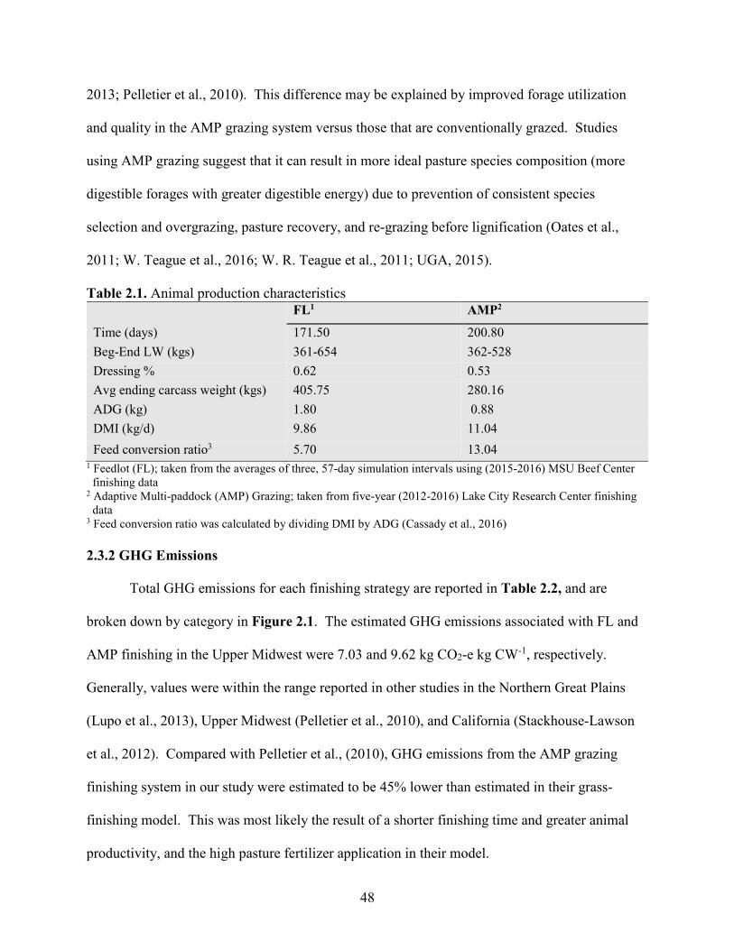
48

2013; Pelletier et al., 2010). This difference may be explained by improved forage utilization

and quality in the AMP grazing system versus those that are conventionally grazed. Studies

using AMP grazing suggest that it can result in more ideal pasture species composition (more

digestible forages with greater digestible energy) due to prevention of consistent species

selection and overgrazing, pasture recovery, and re-grazing before lignification (Oates et al.,

2011; W. Teague et al., 2016; W. R. Teague et al., 2011; UGA, 2015).

Table 2.1. Animal production characteristics FL1 AMP2

Time (days) 171.50 200.80

Beg-End LW (kgs) 361-654 362-528

Dressing % 0.62 0.53

Avg ending carcass weight (kgs) 405.75 280.16

ADG (kg) 1.80 0.88

DMI (kg/d) 9.86 11.04

Feed conversion ratio3 5.70 13.04 1 Feedlot (FL); taken from the averages of three, 57-day simulation intervals using (2015-2016) MSU Beef Center

finishing data 2 Adaptive Multi-paddock (AMP) Grazing; taken from five-year (2012-2016) Lake City Research Center finishing

data 3 Feed conversion ratio was calculated by dividing DMI by ADG (Cassady et al., 2016)

2.3.2 GHG Emissions

Total GHG emissions for each finishing strategy are reported in Table 2.2, and are

broken down by category in Figure 2.1. The estimated GHG emissions associated with FL and

AMP finishing in the Upper Midwest were 7.03 and 9.62 kg CO2-e kg CW-1, respectively.

Generally, values were within the range reported in other studies in the Northern Great Plains

(Lupo et al., 2013), Upper Midwest (Pelletier et al., 2010), and California (Stackhouse-Lawson

et al., 2012). Compared with Pelletier et al., (2010), GHG emissions from the AMP grazing

finishing system in our study were estimated to be 45% lower than estimated in their grass-

finishing model. This was most likely the result of a shorter finishing time and greater animal

productivity, and the high pasture fertilizer application in their model.

49

Similar to other studies, enteric CH4 contributed the most to overall emissions (Figure

2.1) in AMP. Compared with FL finishing, the AMP grazing scenario generated double the

enteric CH4 emissions, highlighted in Figure 2.1. This emphasizes the benefits of higher energy

feeds and shorter lifetime, resulting in productivity gains in our FL model. Despite the heavy

uncertainty associated with IPCC CH4 accounting, specifically with regards to the use of default

Ym values (Stackhouse-Lawson et al., 2012; Rowntree et al., 2016), we used this method for

consistency with other literature. If, however, we had used the results of Chiavegato et al.

(2015b) estimated from data collected at the MSU Lake City AgBioResearch center, the enteric

CH4 footprint in our AMP grazing model would have been reduced by 35%, representing a

decrease from 1,434 to 1,030 kg CO2-e steer-1 (Table A.3.). Similarly, if Ym had been reduced

from the default of 6.5+/-1 to 5.5 to reflect improved forage quality, enteric CH4 emissions from

the AMP scenario would have been reduced by 15% (Table A.3.). Therefore, it is likely that the

use of IPCC (2006) enteric CH4 accounting methodology overestimates actual enteric CH4

emissions, especially when high quality forages are grazed. This overestimation has also been

reported in other studies (Rowntree et al., 2016; Stackhouse-Lawson et al., 2012), and reflects

the uncertainty embedded in the use of IPCC methodology to represent a wide variety of diets.

Although less total manure emissions were estimated for the AMP grazing system than

for the FL scenario (6.9 vs 7.3 Mg CO2-e), when reflected on an animal productivity basis (CO2-

e kg CW-1), manure emissions were actually greater than the FL scenario. This is the result of an

elevated DMI and lower overall carcass weight. Manure CH4 and N2O for the FL scenario

estimated by this study were greater than reported by others (Lupo et al., 2013; Pelletier et al.,

2010). Likely, this is attributable to the use of IPCC Tier 2 methodology in the current study

50

instead of Tier 1 employed in other studies, greater precipitation in our study area compared with

others, and handling of manure in the FL as a liquid instead of a solid.

Our feed production emissions in the FL were slightly greater than feed production

emissions reported by Lupo et al. (2013) and Pelletier et al. (2010), likely because our feedlot

ration did not include a high proportion of legume forages and contained a larger portion of

DDGs and corn grains, which according to Gustavo et al. (2013) have greater emissions

compared with other feedstuffs. Additionally, the model employed by Gustavo et al., (2013)

included additional inputs and processes not included in conventional beef production LCAs; for

example, pest management and transportation of inputs. Fertilizer offsets from animal manure is

a common assumption in many beef LCAs, however, they were not included in this study

because all manure collected from the FL was spread on non-feed component cropland.

Considering fertilizer offsets would have reduced our overall GHG footprint from feed

production, and may consequently account for some of the deviation compared with other

studies. Emissions from on-farm energy use and transportation and mineral supplement

production represented a very small portion of total emissions, accounting for <2.5% and

<0.05% of total GHG footprint, respectively.

51

Table 2.2. Greenhouse gas emissions (kg CO2-e) associated with one steer for both adaptive

multi-paddock (AMP) grazing and feedlot (FL) finishing stages for all impact categories and

their percentage of total emissions. GHG emissions (kg CO2-e steer-1) % of total

AMP 2694.64

Enteric CH4 1434.18 53.22%

Manure Emissions 1 688.27 25.54%

Feed Emissions 2 511.95 19.00%

Mineral Supplement Emissions 3 0.76 0.03%

On-farm energy and transportation 59.47 2.21%

kg CW 280.16

Total (kg CO2-e kg CW-1) 9.62

FL 2853.22

Enteric CH4 776.96 27.23%

Manure Emissions 1 732.66 25.68%

Feed Emissions 2 1288.20 45.15%

Mineral Emissions 3 1.34 0.05%

On-farm energy and transportation 54.06 1.89%

kg CW 405.75

Total (kg CO2-e kg CW-1) 7.03

1 Predominately indirect N2O, but also contains manure derived CH4 2 Calculated from respective feed components using Gustavo et al., (2013) 3 Calculated using data from Lupo et al., (2013).

52

Figure 2.1. GHG emissions (kg CO2-e kg CW-1) presented by emissions category for feedlot

(FL) and adaptive multi-paddock (AMP) grazing systems.

2.3.3. Soil C sequestration

When compared with the 2012 baseline (33.97 +/- 0.71 Mg C ha-1 in the top 30 cm,

measured in SL soils), the 2016 soil C stock increased by 15.18, 8.16, and 19.75 Mg C ha-1 in

SL, S, and CL, suggesting a four-year sequestration rate of 3.79, 2.04, and 4.94 Mg C ha-1 yr-1

within the three soil types, respectively. When S, SL and CL soil C stocks were aggregated, and

compared back to 2012 baseline, the mean sequestration rate is 3.59 Mg C ha-1 yr-1 (Table 2.3).

Ideally, we would have preferred to have SOC across each soil type in 2012, but those data were

not available. However, given that the 2016 SL mean C contents are centric to overall on-farm

SOC stocks when comparing to S and CL, we assumed for the purposes of this analysis that the

SL soil C contents from 2012 were representative of the overall farm. Further, estimating

sequestration rates using average values across all soil types from 2016 yielded a slightly lower

0 1 2 3 4 5 6 7 8 9 10 11

Total

Mineral Emissions

On-farm energy and transportation

Manure Emissions

Feed Emissions

Enteric CH₄

GHG Emissions (kg CO2-e kg CW-1 )

FL AMP

53

rate than when using the 2016 SL data only. Therefore, we determined that using the 2012 SL

samples as a baseline for the full field is more conservative and robust for our estimations.

Our estimated sequestration rate (3.59 Mg C ha-1 yr-1 ) is considerably greater than the

mean C sequestration rate of 0.41 Mg C ha-1 yr-1 for improved grazing reported by Conant et al.,

(2003). However, as indicated by Minasny et al. (2017), these numbers are more than 14 years

old and may not accurately represent new understanding of soil C based on more dynamic soil

and grazing models. Similar to the management in our study, Wang et al. (2015) reported 3.53

Mg C ha-1 yr-1 C sequestration for pastures transitioned from heavy continuous to AMP grazing

in Northern Texas. This value is more consistent with our four-year sequestration rate of 3.59

Mg C ha-1 yr-1.

Studies indicating projected saturation rates based on older soil C stock data suggest that

our soils in the Upper Midwest are approaching saturation based on existing soil C stocks.

However, because soils that are farther away from soil C saturation will accumulate C more

quickly than soils near saturation, and because our estimated soil C sequestration rate is much

higher than the 0.41 Mg C ha-1 yr-1 indicated by Conant et al. (2003), we hypothesize that our

soils will continue to sequester C efficiently for an extended period before reaching saturation

(Minasny et al., 2017; Stewart et al., 2007).

Alternatively, for the FL scenario, there was no C sequestration because intensively

cropped soils associated with feed production are often heavily eroded (Olson et al., 2017).

However, there is considerable opportunity for sustainability improvements on these croplands

through different agronomic practices such as leaving crop residues, increased perennials in

rotations, conservation and no-till, cover crops, and increased use of organic amendments such as

compost (Chambers et al., 2016; Minasny et al., 2017). If adopted, these practices may also

54

promote soil C sequestration (Chambers et al., 2016). Nevertheless, studies indicate that in

general, grasslands continue to sequester C at higher rates than improved cropland, and that

transitions from cropland to grassland show the greatest rates of C sequestration, in some cases

as high as 8.0 Mg C ha-1 yr-1 (Machmuller et al., 2015; Mathew et al., 2017; Minasny et al.,

2017; Powlson et al., 2011).

Table 2.3. Differences in soil C stock by year and soil type (top) and 4-year soil C sequestration

rates by and across soil types (bottom). Soil C Stock (Mg C ha1)

20122 20163

Soil Type4 Mean Std Error Mean Std Error

S - - 42.13 1.59

SL 33.97 0.71 49.15 6.55

CL

Across Type

-

-

-

-

53.72

48.33

7.33

1.95

Soil C Sequestration (Mg C ha=1 yr-1)

Soil Type5 4-year difference Sequestration rate Mean Std Error

S 8.16 2.04 - -

SL 15.18 3.79 - -

CL

Across Type

19.75

14.36

4.94

3.59

-

3.59

-

0.84

1 Represents the average composited 0-30 cm depth of all three replicates, for which ten subsamples were taken

for each replicate and depth 2 All samples collected in 2012 were from sandy loam soils. Average was taken for 2012 Period 2, SysA (data not

shown) from (Chiavegato et al., 2015c) 3 Farm samples from all three soil types were collected 4 SL represents sandy loam, S represents sandy, and CL represents clay loam soil types 5 Compared with the soil stock of sandy loam soils in 2012

2.3.4. Net GHG flux

Soil erosion contributed an additional 113.81 kg CO2-e (0.17 kg CO2 kg CW-1) to the FL

model. Zero soil erosion was assumed for the AMP scenario because our data indicated active C

sequestration over the four-year interval measured in the land associated with this management.

According to (Olson et al., 2016) soil that is not part of a stable aggregate and is eroding cannot

be actively sequestering C. Although soil erosion only contributed modestly to GHG emissions,

soil erosion magnified by intensive cropping systems has important negative impacts on other

55

ecosystem services that are vital to food production, water quality, nutrient cycling and habitat

support (Olson et al., 2017).

On a CO2-e basis, total sequestration equaled -17.54 kg CO2-e for the AMP grazing

finishing scenario. Combined with 9.62 kg CO2-e kg CW-1 in emissions, this resulted in a net

GHG sink of -7.92 kg CO2-e kg CW-1 (Figure 2.2). Subsequently, the 7.03 kg CO2-e kg CW-1 of

FL emissions combined with 0.17 kg CO2-e kg CW-1 from erosion resulted in a net emission of

7.20 kg CO2-e kg CW-1 for the FL scenario (Figure 2.2). In beef LCA studies from the Northern

Great Plains and the Upper Midwest where soil C sensitivity was included, sequestration rates of

0.41 and 0.12 Mg C ha-1 yr-1 reduced emissions of grass-fed beef production by 24 and 30%,

respectively (Lupo et al., 2013; Pelletier et al., 2010). While these studies were models

generated from the literature, our model used five years of actual finishing data derived from

Lake City AgBioResearch center, and four years of soil C data in paddocks where cattle were

managed by AMP grazing. Therefore, long-term grazing-finishing projections in the Upper

Midwest could be considerably more sustainable than previously thought. This calls into

question the common assumption that intensification reduces overall GHG footprint through

higher productivity. This study shows that when full consideration of land impacts is given to

the GHG emissions in both grain and grazing-based production, the environmental benefits may

outweigh the productivity losses.

56

Figure 2.2. Emissions for each finishing strategy, adaptive multi-paddock (AMP) grazing and

feedlot (FL), are reported for before and after soil C flux is considered. Bars on the left represent

all emissions calculated through the LCA. Bars on the right represent net GHG flux after

incorporation of soil carbon sequestration sinks and soil erosion additions on a CO2-e basis.

Generally, because of the large enteric CH4 footprint, grazing systems have been pointed

to as the greatest area for attention in terms of GHG footprint in beef production. However,

measurements of actual SOC have not been factored into these outcomes. In fact, if soil C

sequestration is achieved through best management practices, enteric CH4 from the finishing

stage can be substantially mitigated. We demonstrate this based on soil C collection from Lake

City AgBioResearch center from 2012-2016, which indicates a -7.92 kg CO2-e kg CW-1 sink.

Therefore, our results in Figure 2.2 are considerably different than current literature and

document the need to consider emissions and sinks from the entire system, including the soil

ecosystem, when modelling beef production systems.

9.6

2

-7.9

2

7.0

3

7.2

0

-10

-8

-6

-4

-2

0

2

4

6

8

10

12

Without Soil C Flux With Soil C flux

kg C

O2-e

kg C

W-1

Net GHG Flux

AMP FL

57

2.4. Conclusions

Using a standard LCA approach in combination with inclusion of soil C accounting, this

study calculated net GHG emissions of two beef finishing systems in the Upper Midwest: feedlot

and adaptive multi-paddock grazing. There are several important literature contributions arising

from this. First, the incorporation of environmental influence of AMP grazing compared with

continuous grazing, the common grass-fed management system utilized by most LCAs, yields

considerably greater food provisioning with different environmental outcomes including a

significant C-sink, which can offset enteric CH4. Second, integrating on-farm soil C data within

the studied management system contributes significantly to the current gap in the literature. To

date, this is the first study that aims to address this gap. In doing so, our results show that not

only can adoption of improved grazing management support soil C sequestration, but that this

production system may serve as an overall GHG sink, likely for years into the future.

There are considerable implications emerging from this study, both for beef production

and for climate change policy. According to West et al., (2014), an additional four billion people

could be fed globally if livestock did not compete for arable cropland that could be used directly

to produce human-edible food. However, existing beef LCAs suggest movement into grass-

based beef production would drastically reduce energy efficiency and food production, while

significantly increasing CH4 emissions and needed land-area (Capper, 2012). Our results are

contrary to this view. Potentially, an AMP grazing system can be a win-win scenario with

marked increased in beef production per unit land when compared to LCAs in the existing

literature, while also improving ecosystem services. Therefore, AMP has great potential to meet

food production challenges as population projections increase while potentially improving the

natural resource base human life depends on.

58

Continued investigation of AMP grazing in large-scale landscape trials across multiple

ecoregions differing in climate and plant species mixes is warranted and necessary to best apply

this strategy to local and regional conditions.

59

APPENDIX

60

A.1. Feedlot Simulation Calculations

An extension from a 90-day finishing research experiment to an industry representative

170-day finishing period was simulated (Table A.1). Dry matter intake (DMI) was calculated

from NRC (2016) Eq. 10-4 as

���,��

�= 3.830 + 0.0143 � ����

where ISBW is initial shrunk body weight (kg), calculated from live weight upon entrance into

the FL. This equation is used for steers fed high-grain diets with NEg greater than 1.4 Mcal kg

NEg-1. This equation was chosen for our methods because the NEg used in our feedlot ration was

1.46 Mcal kg NEg-1. NEm required was calculated following NRC (2016) Eq. 11-1 as

��� = 0.077 ����.��

where SBW is shrunk body weight. This was divided by actual NEm consumed in the ration to

determine feed required for maintenance. Thus, NEg required was calculated as

��� ��� !��� "#� �$!% = &��� − "��� ��� !��� "#� �$!%(�%$%)�* � ��� )#%+ ���

where feed required for maintenance is in kg DM. Average daily gain (ADG) was extrapolated

from NRC (2016) table 12-1 using the NRC (1984) equation

��� = 0.0493 � ��.��� -�./.�0�

where W is weight (kg) and LWG is live weight gain.

Therefore, for each 57-day interval, weight gain was calculated, added to the weight at

the beginning of the interval, and used as the beginning weight for the next interval. Feed

composition is represented in Table A.2.

61

Table A.1. Feedlot simulation, broken down into three, 57-day intervals for both 2015 and 2016.

F1: Days 1-57 F2: Days 58-114 F3: Days 115-171

Production Measure 2015 2016 2015 2016 2015 2016

Entry SBW1 351.41 343.57 458.00 451.87 560.60 554.47

NEg consumed2 (Mcal kg d-1) 1.45 1.48 1.45 1.48 1.45 1.48

DMI3 (kg d-1) 8.41 8.29 9.93 9.84 11.40 11.31

NEm required4 (Mcal kg d-1) 6.25 6.14 7.62 7.55 8.87 8.80

NEm consumed2 (Mcal kg DM-1) 2.13 2.16 2.13 2.16 2.13 2.16

Feed req. for maintenance (kg DM) 2.93 2.85 3.57 3.50 4.16 4.08

NEg required5 (Mcal d-1) 7.97 8.05 9.25 9.38 10.53 10.69

Shrunk ADG6 (kg) 1.87 1.90 1.80 1.80 1.70 1.70

Weight gained (kg) 106.59 108.30 102.60 102.60 96.90 96.90

End weight (kg) 458.00 451.87 560.60 554.47 657.50 651.37

1 Represents liveweight at entry into the feedlot (on-farm data) minus 4% conversion to shrunk body weight (SBW) 2 Energy composition of actual TMR 3 Calculated using NRC (2016) Eq. 10-4 4 Calculated using NRC (2016) Eq. 11-1 5 Calculated using NRC (2016), pg. 190 6 Calculated using NRC (2016) table 12-1

Table A.2. Actual on-farm feed components. Feed composition and weights fed during the 90-

day trial were scaled up based on the projected feed needed for each interval of the simulation

and multiplied by the percentage that each feed component represented in the original ration.

Year

Feed component (kg DM) 2015 2016

Corn silage 158.56 282.38

DDGs 760.98 208.22

HMC 311.00 1144.65

Corn grain1 399.59

Alfalfa hay 64.55 43.03

Total 1694.67 1678.29 1 Corn grain was only fed in 2015. In 2016, this was compensated with increased corn silage and HMC.

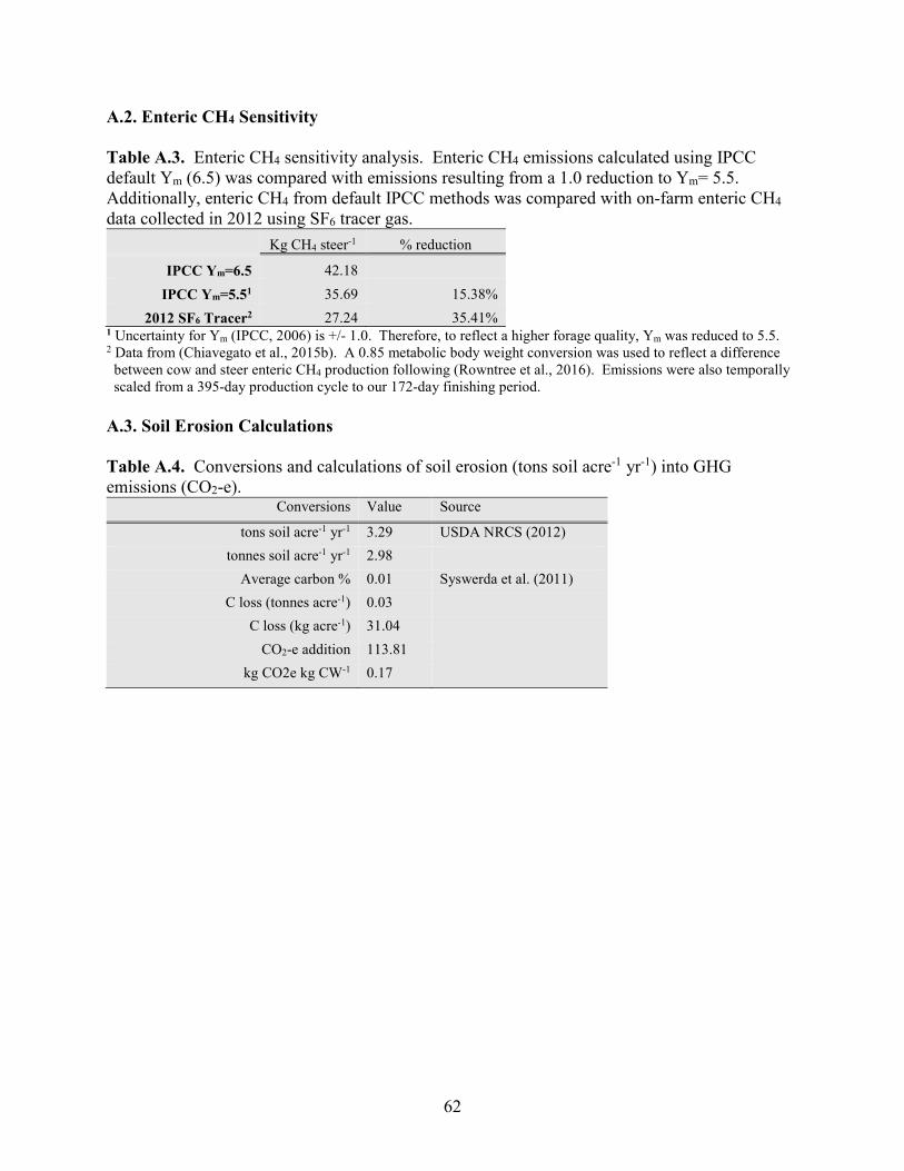
62

A.2. Enteric CH4 Sensitivity

Table A.3. Enteric CH4 sensitivity analysis. Enteric CH4 emissions calculated using IPCC

default Ym (6.5) was compared with emissions resulting from a 1.0 reduction to Ym= 5.5.

Additionally, enteric CH4 from default IPCC methods was compared with on-farm enteric CH4

data collected in 2012 using SF6 tracer gas.

Kg CH4 steer-1 % reduction

IPCC Ym=6.5 42.18

IPCC Ym=5.51 35.69 15.38%

2012 SF6 Tracer2 27.24 35.41% 1 Uncertainty for Ym (IPCC, 2006) is +/- 1.0. Therefore, to reflect a higher forage quality, Ym was reduced to 5.5. 2 Data from (Chiavegato et al., 2015b). A 0.85 metabolic body weight conversion was used to reflect a difference

between cow and steer enteric CH4 production following (Rowntree et al., 2016). Emissions were also temporally

scaled from a 395-day production cycle to our 172-day finishing period.

A.3. Soil Erosion Calculations

Table A.4. Conversions and calculations of soil erosion (tons soil acre-1 yr-1) into GHG

emissions (CO2-e). Conversions Value Source

tons soil acre-1 yr-1 3.29 USDA NRCS (2012)

tonnes soil acre-1 yr-1 2.98

Average carbon % 0.01 Syswerda et al. (2011)

C loss (tonnes acre-1) 0.03

C loss (kg acre-1) 31.04

CO2-e addition 113.81

kg CO2e kg CW-1 0.17

63

LITERATURE CITED

64

LITERATURE CITED

Beef2Live. (2017). World Beef Production: Ranking Of Countries. Retrieved from

http://beef2live.com/story-world-beef-production-ranking-countries-0-106885

Brilli, L., Bechini, L., Bindi, M., Carozzi, M., Cavalli, D., Conant, R., . . . Farina, R. (2017).

Review and analysis of strengths and weaknesses of agro-ecosystem models for

simulating C and N fluxes. Science of the Total Environment, 598, 445-470.

Capper, J. L. (2012). Is the Grass Always Greener? Comparing the Environmental Impact of

Conventional, Natural and Grass-Fed Beef Production Systems. Animals: an open access

journal from MDPI, 2(2), 127-143.

Cassady, C. J., Felix, T. L., Beever, J. E., and Shike, D. W. (2016). Effects of timing and

duration of test period and diet type on intake and feed efficiency of Charolais-sired

cattle. Journal of Animal Science, 94(11), 4748.

Chambers, A., Lal, R., & Paustian, K. (2016). Soil carbon sequestration potential of US

croplands and grasslands: Implementing the 4 per Thousand Initiative. Journal of Soil

and Water Conservation, 71(3), 68A-74A.

Chiavegato, M. B., Rowntree, J., Powers, W. J., and Carmichael, D. (2015a). Pasture-derived

greenhouse gas emissions in cow-calf production systems. Journal of Animal Science,

93(3), 1350.

Chiavegato, M. B., Rowntree, J., Powers, W. J., and Carmichael, D. (2015b). Enteric methane

from lactating beef cows managed with high- and low-input grazing systems. Journal of

Animal Science, 93(3), 1365-1375.

Chiavegato, M. B., Rowntree, J., Powers, W. J., and Carmichael, D. (2015c). Carbon flux

assessment in cow-calf grazing systems. Journal of Animal Science, 93(8), 4189-4199.

Conant, R. T., Six, J., and Paustian, K. (2003). Land use effects on soil carbon fractions in the

southeastern United States. I. Management-intensive versus extensive grazing. Biology

and Fertility of Soils, 38(6), 386-392.

Cook, R., and Weller, D. (2004). In defense of crop monoculture. Paper presented at the

Proceedings 4th International Crop Science Congress’.(The Regional Institute Ltd:

Gosford, NSW) Available at:

www.cropscience.org.au/icsc2004/symposia/2/1/1128_cookrj. htm.

FAO. (2012). Livestock and Landscapes. Food and Agriculture Organization of the United

Nations.

65

Gerber, P. J., Steinfeld, H., Henderson, B., Mottet, A., Opio, C., Dijkman, J., Falcucci, A. and

Tempio, G. (2013). Tackling climate change through livestock: a global assessment of

emissions and mitigation opportunities. Retrieved from Rome.

Gerrish, J. (2004). Management-Intensive Grazing: The Grassroots of Grass Farming: Green

Park Press.

Gustavo, G. T. C., Ryan, M. R., and Richard, T. L. (2013). Energy Use and Greenhouse Gas

Emissions from Crop Production Using the Farm Energy Analysis Tool. BioScience,

63(4), 263-273.

Hall, C. A. S., Pimentel, D., and Dale, B. E. (2011). Seeking to Understand the Reasons for

Different Energy Return on Investment (EROI) Estimates for Biofuels. Sustainabilitty,

3(12), 2413-2432.

IPCC. (2006). IPCC Guidelines for Greenhouse Gas Inventories. Retrieved from

http://www.ipcc-

nggip.iges.or.jp/public/2006gl/pdf/4_Volume4/V4_10_Ch10_Livestock.pdf

IPCC. (2014). Anthropogenic and Natural Radiative Forcing. In G. Myhre, D. Shindell, F.-M.

Bréon, W. Collins, J. Fuglestvedt, J. Huang, D. Koch, J.-F. Lamarque, D. Lee, B.

Mendoza, and A. R. T. Nakajima, G. Stephens, T. Takemura and H. Zhang (Eds.),

Climate Change 2013: The Physical Science Basis. Contribution of Working Group I to

the Fifth Assessment Report of the Intergovernmental Panel on Climate Change:

Cambridge University Press.

Janzen, H. H. (2011). What place for livestock on a re-greening earth? Animal Feed Science and

Technology, 166, 783-796.

Kim, S., and Dale, B. E. (2008). Life cycle assessment of fuel ethanol derived from corn grain

via dry milling. Bioresource Technology, 99(12), 5250-5260.

Liebig, M. A., Gross, J. R., Kronberg, S. L., Phillips, R. L., and Hanson, J. D. (2010). Grazing

management contributions to net global warming potential: a long-term evaluation in the

Northern Great Plains. Journal of Environmental Quality, 39(3), 799-809.

Lupo, C. D., Clay, D. E., Benning, J. L., and Stone, J. J. (2013). Life-Cycle Assessment of the

Beef Cattle Production System for the Northern Great Plains, USA. Journal of

Environmental Quality, 42(5), 1386-1394.

Machmuller, M. B., Kramer, M. G., Cyle, T. K., Hill, N., Hancock, D., and Thompson, A.

(2015). Emerging land use practices rapidly increase soil organic matter. Nature

Communications, 6, 6995.

66

Mathew, I., Shimelis, H., Mutema, M., and Chaplot, V. (2017). What crop type for atmospheric

carbon sequestration: Results from a global data analysis. Agriculture Ecosystems &

Environment, 243, 34-46.

McSherry, M. E., and Ritchie, M. E. (2013). Effects of grazing on grassland soil carbon: a global

review. Global Change Biology, 19(5), 1347-1357.

Minasny, B., Malone, B. P., McBratney, A. B., Angers, D. A., Arrouays, D., Chambers, A., . . .

Winowiecki, L. (2017). Soil carbon 4 per mille. Geoderma, 292, 59-86.

National Academies of Sciences, E. a. M. (2016). Nutrient Requirements of Beef Cattle (Vol.

Eighth Revised Edition). Washington, DC: National Academies Press.

Oates, L. G., Undersander, D. J., Gratton, C., Bell, M. M., and Jackson, R. D. (2011).

Management-Intensive Rotational Grazing Enhances Forage Production and Quality of

Subhumid Cool-Season Pastures. Crop Science, 51(2), 892-901.

OECD. (2016). Meat Consumption. Retrieved from https://data.oecd.org/agroutput/meat-

consumption.htm

Olson, K. R., Al-Kaisi, M., Lal, R., and Cihacek, L. (2016). Impact of soil erosion on soil

organic carbon stocks. Journal of Soil and Water Conservation, 71(3), 61-67A.

Olson, K. R., Al-Kaisi, M., Lal, R., and Morton, L. W. (2017). Soil ecosystem services and

intensified cropping systems. Journal of Soil and Water Conservation, 72(3), 64A-69A.

Pelletier, N., Pirog, R., and Rasmussen, R. (2010). Comparative life cycle environmental impacts

of three beef production strategies in the Upper Midwestern United States. Agricultural

Systems, 103(6), 380-389.

Powlson, D. S., Whitmore, A. P., and Goulding, K. W. T. (2011). Soil carbon sequestration to

mitigate climate change: a critical re-examination to identify the true and the false.

European Journal of Soil Science, 62(1), 42-55.

Rochette, P., Worth, D. E., Lemke, R. L., McConkey, B. G., Pennock, D. J., Wagner-Riddle, C.,

and Desjardins, R. (2008). Estimation of N2O emissions from agricultural soils in

Canada. I. Development of a country-specific methodology. Canadian Journal of Soil

Science, 88(5), 641-654.

Rowntree, J. E., Ryals, R., DeLonge, M., Teague, W. R., Chiavegato, M., Byck, P., . . . Xu, S.

(2016). Potential mitigation of midwest grass-finished beef production emissions with

soil carbon sequestration in the United States of America. Future of Food: Journal on

Food, Agriculture and Society, 4(3), 31-38.

Ryan, B., and Tiffany, D. G. (1998). Energy use in Minnesota agriculture. Minnesota

Agricultural Economist(693), 1, 4-7.

67

Savory, A., Butterfield, J. (1998). Holistic Management: A New Framework for Decision Making

(2nd ed.): Island Press.

Schader, C., Muller, A., Scialabba, N. E.-H., Hecht, J., Isensee, A., Erb, K.-H., . . . Niggli, U.

(2015). Impacts of feeding less food-competing feedstuffs to livestock on global food

system sustainability. Journal of the Royal Society, Interface / the Royal Society, 12(113).

Schroeder, J. W. (2012). Weights and Measures of Common Feeds. Retrieved from

https://www.ag.ndsu.edu/pubs/ansci/livestoc/as1282.pdf

Sloggett, G. (1992). Estimating Energy Use in World Irrigation. In R. Fluck (Ed.), Energy in

Farm Production (Vol. 6): Institute of Food and Agricultural Sciences.

Stackhouse-Lawson, K. R., Rotz, C. A., Oltjen, J. W., and Mitloehner, F. M. (2012). Carbon

footprint and ammonia emissions of California beef production systems. Journal of

Animal Science, 90(12), 4641-4655.

Stewart, C. E., Paustian, K., Conant, R. T., Plante, A. F., and Six, J. (2007). Soil Carbon

Saturation: Concept, Evidence and Evaluation. Biogeochemistry, 86(1), 19-31.

Syswerda, S. P., Corbin, A. T., Mokma, D. L., Kravchenko, A. N., and Robertson, G. P. (2011).

Agricultural Management and Soil Carbon Storage in Surface vs. Deep Layers. Soil

Science Society of America Journal, 75(1), 92-101.

Teague, W., Apfelbaum, S., Lal, R., Kreuter, U., Rowntree, J., Davies, C., . . . Wang, T. (2016).

The role of ruminants in reducing agriculture's carbon footprint in North America.

Journal of Soil and Water Conservation, 71(2), 156-164.

Teague, W. R., Dowhower, S. L., Baker, S. A., Haile, N., DeLaune, P. B., and Conover, D. M.

(2011). Grazing management impacts on vegetation, soil biota and soil chemical,

physical and hydrological properties in tall grass prairie. Agriculture, Ecosystems and

Environment, 141(3), 310-322.

UGA. (2015). What Is Management-Intensive Grazing? Retrieved from

http://www.caes.uga.edu/topics/sustainag/grazing/

USDA. (2012). Sheet, Rill and Wind Erosion.

USDA. (2014). 2012 Census of Agriculture.

USDA. (2015a). Crop Production. National Agricultural Statistics Service.

USDA. (2015b). Summary Report: 2012 National Resources Inventory. Center for Survey

Statistics and Methodology.

68

USDA. (2016a). Corn Background. Retrieved from

http://www.ers.usda.gov/topics/crops/corn/background.aspx

USDA. (2016b). Overview of the United States Cattle Industry.

Voisin, A. (1959). Grass Productivity: Island Press.

Wang, T., Teague, W. R., Park, S. C., and Bevers, S. (2015). GHG Mitigation Potential of

Different Grazing Strategies in the United States Southern Great Plains. Sustainability,

7(10), 13500-13521.

West, P. C., Gerber, J. S., Engstrom, P. M., Mueller, N. D., Brauman, K. A., Carlson, K. M., . . .

Siebert, S. (2014). Leverage points for improving global food security and the

environment. Science (New York, N.Y.), 345(6194), 325-328.

69

CHAPTER 3

CONCLUSIONS AND FUTURE RESEARCH

70

The results of this study indicate that AMP grazing can potentially sequester SOC and

offset GHG emissions for the finishing stage of beef production in the Upper Midwest.

However, other stages of cattle production also emit GHGs and can have negative environmental

impacts. Namely, the cow-calf stage contributes most to cradle-to-gate emissions. Although we

only examined the impacts of AMP grazing compared with the feedlot system in the finishing

stage, this production strategy can also be implemented in the cow-calf stage and therefore may

result in further GHG mitigation. Studies examining the environmental impacts for the entire

cradle-to-gate lifespan of cattle using AMP grazing throughout would be warranted.

In this study, we were lucky to have one of the few longer term SOC data sets including

baseline SOC stocks for our perusal. Moving forward, to continue to include SOC as an

environmental indicator into beef-cattle LCAs in other eco-regions, more robust SOC accounting

and datasets will be absolutely vital. It is possible that the sequestration rate observed in this

study may not apply in other climates (i.e., in more arid regions), other soil types, and different

plant species combinations where SOC sequestration capacity is limited. Results of such

information could influence the regionality of beef production in the future, and possibly be

instrumental in creating production systems in which beef production is only sustained in areas

where its environmental impacts may be more optimally compensated for with SOC

sequestration.

Another important area of further research is the study of additional ecosystem services

that are underrepresented by the current LCA literature. Aside from GHG emissions, beef

production can result in environmental impacts that include deforestation and land-use change,

soil health impacts such as water holding capacity, biodiversity and cation exchange capacity,

marine and freshwater eutrophication, and soil erosion and sedimentation. These ecosystem

71

services are often hard to understand and may have a variety of effects, making them both

difficult to study and to include in LCA. However, considering that these ecosystem services

have a multitude of both environmental and economic benefits (i.e., food provisioning, nutrient

cycling, water infiltration and ecosystem resiliency), they represent an important area of needed

study in the future. Full-cost accounting is one method to incorporate these impacts.

Monetization of externalized costs borne by beef production and antecedent feed production may

present an opportunity to examine these impacts on a dollar basis, which may generate a holistic

indicator of sustainability further than what can be deduced currently based only on GHG

emissions.

Lastly, the environmental improvements that may be generated through AMP grazing are

strictly hypothetical if this practice is not more widely adopted in the future. Even though we

have some evidence, scientifically, what these practices may contribute to environmental

preservation and GHG mitigation, policy implications are hard to understand and are often not

the focus of implicative research. It is vital for scientific findings, such as those presented in this

study, to influence environmental and agricultural policy in the future. Currently, continuous

grazing is the most common “grass-fed” technique, globally, while conventional feedlot

finishing is the most common production technique domestically. However, if one goal is to

increase the scale of adoption of regenerative and less environmentally harmful practices, such as

AMP grazing, we must better understand two things: 1) how these research findings may

translate into policy; and, 2) how these policies will impact food security, consumer perception,

and farmer adoptability.

Knowledge gained from more robust soil C datasets and ecosystem service dynamics will

help formulate sound policy regarding beef production practices. Additionally, future research

72

may give light to cropping mechanisms and systems that may result in greater soil formation and

SOC sequestration. Even if soil C saturation does limit the time-scale that AMP grazing will

provide a GHG sink, the possibility that it may serve as a short-run mitigation technique while

better renewable energy technologies are developed, remains a critically important consideration

and potentially viable alternative.