Embed Size (px)
Citation preview
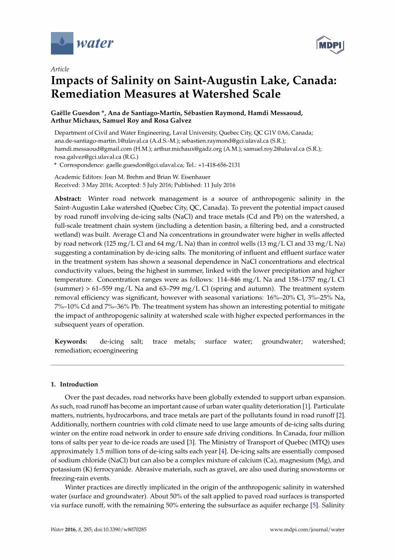
water
Article
Impacts of Salinity on Saint-Augustin Lake, Canada:Remediation Measures at Watershed ScaleGaëlle Guesdon *, Ana de Santiago-Martín, Sébastien Raymond, Hamdi Messaoud,Arthur Michaux, Samuel Roy and Rosa Galvez
Department of Civil and Water Engineering, Laval University, Quebec City, QC G1V 0A6, Canada;[email protected] (A.d.S.-M.); [email protected] (S.R.);[email protected] (H.M.); [email protected] (A.M.); [email protected] (S.R.);[email protected] (R.G.)* Correspondence: [email protected]; Tel.: +1-418-656-2131
Academic Editors: Joan M. Brehm and Brian W. EisenhauerReceived: 3 May 2016; Accepted: 5 July 2016; Published: 11 July 2016
Abstract: Winter road network management is a source of anthropogenic salinity in theSaint-Augustin Lake watershed (Quebec City, QC, Canada). To prevent the potential impact causedby road runoff involving de-icing salts (NaCl) and trace metals (Cd and Pb) on the watershed, afull-scale treatment chain system (including a detention basin, a filtering bed, and a constructedwetland) was built. Average Cl and Na concentrations in groundwater were higher in wells affectedby road network (125 mg/L Cl and 64 mg/L Na) than in control wells (13 mg/L Cl and 33 mg/L Na)suggesting a contamination by de-icing salts. The monitoring of influent and effluent surface waterin the treatment system has shown a seasonal dependence in NaCl concentrations and electricalconductivity values, being the highest in summer, linked with the lower precipitation and highertemperature. Concentration ranges were as follows: 114–846 mg/L Na and 158–1757 mg/L Cl(summer) > 61–559 mg/L Na and 63–799 mg/L Cl (spring and autumn). The treatment systemremoval efficiency was significant, however with seasonal variations: 16%–20% Cl, 3%–25% Na,7%–10% Cd and 7%–36% Pb. The treatment system has shown an interesting potential to mitigatethe impact of anthropogenic salinity at watershed scale with higher expected performances in thesubsequent years of operation.
Keywords: de-icing salt; trace metals; surface water; groundwater; watershed;remediation; ecoengineering
1. Introduction
Over the past decades, road networks have been globally extended to support urban expansion.As such, road runoff has become an important cause of urban water quality deterioration [1]. Particulatematters, nutrients, hydrocarbons, and trace metals are part of the pollutants found in road runoff [2].Additionally, northern countries with cold climate need to use large amounts of de-icing salts duringwinter on the entire road network in order to ensure safe driving conditions. In Canada, four milliontons of salts per year to de-ice roads are used [3]. The Ministry of Transport of Quebec (MTQ) usesapproximately 1.5 million tons of de-icing salts each year [4]. De-icing salts are essentially composedof sodium chloride (NaCl) but can also be a complex mixture of calcium (Ca), magnesium (Mg), andpotassium (K) ferrocyanide. Abrasive materials, such as gravel, are also used during snowstorms orfreezing-rain events.
Winter practices are directly implicated in the origin of the anthropogenic salinity in watershedwater (surface and groundwater). About 50% of the salt applied to paved road surfaces is transportedvia surface runoff, with the remaining 50% entering the subsurface as aquifer recharge [5]. Salinity
Water 2016, 8, 285; doi:10.3390/w8070285 www.mdpi.com/journal/water

Water 2016, 8, 285 2 of 19
has a significant impact on water ecosystems, producing toxicity to benthic and other freshwaterorganisms and affecting invertebrate reproduction [6]. As reported by Novotny and Stefan [7], de-icingsalts can modify lake stratification and indirectly aggravate lake eutrophication processes by extendinganoxia conditions and allowing the release of phosphates from organic sediment. The increase of saltconcentration in groundwater is a concern for drinking water [8]. A high proportion of salts can alsobe accumulated in roadside soils and vegetation [9], which can affect soil physicochemical properties,biogeochemical cycles, and soil ecology. In addition, road runoff includes toxic trace metals such as Cdand Pb [10]. Indeed de-icing salts have a strong ability to increase trace metal mobility [11]. In addition,long-term use of de-icing salts can induce problems associated with chloride-induced corrosion ofautomobiles and road infrastructure (highway components, steel reinforcement bars, and concrete)and accelerates pavement deterioration due to freezing and thawing cycles [12]. Despite de-icing saltsnegative impact on the environment in the short and long term [13,14], at present it is difficult to stopor reduce its use for safety reasons. Therefore, strategies are aimed at preventing the potential impactcaused from road runoff by reducing pollutant concentration. Nowadays, there are various strategiesincluding constructed wetlands, oil and grit separators, and storm-water ponds, which are normallypart of a treatment chain system [15]. However, few of these systems target the removal of de-icingsalts from road runoff.
The 1970s construction of a road section of the Felix-Leclerc Highway A40 near Quebec City(Canada) has greatly contributed to water quality degradation in the Saint-Augustin Lake watershed.Several studies show that Saint-Augustin Lake water quality is being compromised by theincreased human settlements around the watershed [16–18]. The proximity of the Highway A40to Saint-Augustin Lake has induced surface water, groundwater, and sediment pollution by roadde-icing salts and trace metals. Indeed, different water and sediment quality changes in Saint-AugustinLake were observed after the Highway A40 construction: (i) high electrical conductivity (0.7–1.3 dS/m)in surface water was recorded with a positive relation with Na and Cl ions [10]; (ii) saltwater algaespecies are now present in the lake [17]; and (iii) high trace metal concentrations were measured insediments [19]. Moreover, after the construction of the Highway A40, high electrical conductivityvalues and NaCl concentrations in groundwater were reported [20]. In order to mitigate the impacts ofde-icing salts on water quality in the Saint-Augustin Lake watershed, a full-scale chain system to treatroad runoff from Highway A40 was constructed. The treatment chain system was built in 2011 andincludes a detention basin, an active filtering bed and an adapted constructed wetland.
This work concerns a field research project that includes the design of the system, its constructionand monitoring program to evaluate groundwater and surface water quality in the Saint-AugustinLake watershed, as well as system performance in the first and second years of operation. Specificdiscussion is made on the temporal variation patterns of NaCl and trace metals (Cd and Pb), and otherwater quality indicators (temperature, pH, electrical conductivity, and suspended solids).
2. Materials and Methods
2.1. Site Description
The water quality monitoring was conducted from spring 2012 to autumn 2013 in Saint-AugustinLake watershed (flood plain of St. Laurent River, Saint-Augustin-de-Desmaures, QC, Canada), locatedin the municipal limit of Saint-Augustin-de-Desmaures (40 m altitude). The Saint-Augustin Lakewatershed is located about 15 km in the west of Quebec City (Canada) and has an area of 7.64 km2
(Figure 1). Saint-Augustin Lake has a maximum dimension of 2.1 km in length, 0.3 km in width [21] anda depth average of 3.5 m [19]. The water renewal rate is estimated at 6 months and it is mainly driven bygroundwater inflow [10]. Average annual temperature is 5.1 ˝C and total annual precipitation (rainfall+ water equivalent of the total snow) is 1109 mm/year for the 1998–2012 period (Station Jean Lesage,Quebec City, QC, Canada) [22]. The Saint-Augustin Lake watershed is included in two geologicalformations of the Paleozoic. The north-northwest of the watershed, including the lake is in the St.

Water 2016, 8, 285 3 of 19
Lawrence Platform formation, upper and middle Ordovician. This formation is characterized by arock composed of Mudrock, slate, dolomite and sandstone. The south part of the watershed is in theAppalachians Province, Ordovician to lower Silurian characterized by a rock composed of shale.
Water 2016, 8, 285 3 of 19
formation is characterized by a rock composed of Mudrock, slate, dolomite and sandstone. The south
part of the watershed is in the Appalachians Province, Ordovician to lower Silurian characterized by
a rock composed of shale.
Figure 1. Groundwater sampling wells in Saint‐Augustin Lake watershed (Quebec) and geological
context. Red stars represent groundwater sampling wells: G1 (road control); G2 (residential control);
and G3 to G5 (study wells affected by road and residential areas). Pilot site to runoff desalination is
also indicated in the picture.
From 1960 onwards, population and land use have markedly changed. Conversion of forest to
residential zones has become the dominant land use change. Currently, main land uses are
agriculture, forestry, and residential, being 20%–25%, 20%, and 30% of the total area, respectively. In
1974, a section of Felix‐Leclerc Highway A40 was constructed through part of the watershed (Figure 1)
resulting in an increase in road traffic. Currently, the annual average daily traffic on this section is
around 72,000 vehicles [23], which corresponds to a medium highway [2]. This construction was
accompanied by increased population in the municipality [17]. In last decades, the electrical
conductivity in water of Saint‐Augustin Lake highly increased, coincident with the use of de‐icing
road salts on Highway A40 [10]. With the aim to deal with salt pollution in runoff water, in 2011 an
environmental management solution (hereafter named pilot site) was constructed [24].
2.2. Pilot Site Characteristic
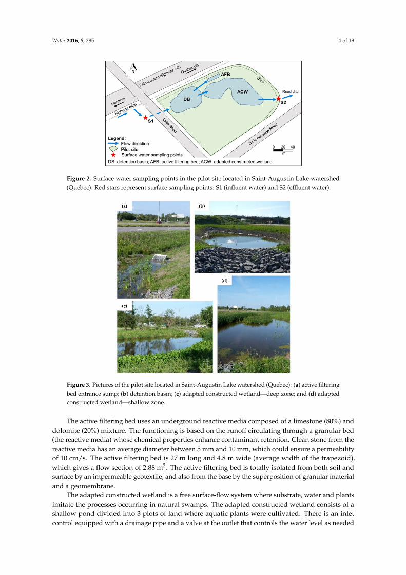
The pilot site is a treatment chain system composed of three units (Figure 2): (1) detention basin;
(2) active filtering bed; and (3) free surface‐flow adapted constructed wetland. The units were
designed and constructed in 2011 in order to collect and treat approximately 25% of the Saint‐
Augustin Lake watershed’s runoff water.
The pilot site was constructed within the limits of the Highway A40 ramp at the north of Saint‐
Augustin Lake. The site is compact and well integrated into the landscape with an area of 22,500 m2.
Runoff is collected in a highway drainage ditch and accumulated in the detention basin before being
redirected to the active filtering bed and/or the adapted constructed wetland (Figure 3).
The detention basin plays a role in the homogenization of the water collected from the highway
ditch and in the regulation of flow water to the adapted constructed wetland and the active filtering
bed. The detention basin accumulates road runoff and removes sediments and particles. The
detention basin surface area is 340 m2 and the volume is 880 m3.
Figure 1. Groundwater sampling wells in Saint-Augustin Lake watershed (Quebec) and geologicalcontext. Red stars represent groundwater sampling wells: G1 (road control); G2 (residential control);and G3 to G5 (study wells affected by road and residential areas). Pilot site to runoff desalination isalso indicated in the picture.
From 1960 onwards, population and land use have markedly changed. Conversion of forest toresidential zones has become the dominant land use change. Currently, main land uses are agriculture,forestry, and residential, being 20%–25%, 20%, and 30% of the total area, respectively. In 1974, a sectionof Felix-Leclerc Highway A40 was constructed through part of the watershed (Figure 1) resultingin an increase in road traffic. Currently, the annual average daily traffic on this section is around72,000 vehicles [23], which corresponds to a medium highway [2]. This construction was accompaniedby increased population in the municipality [17]. In last decades, the electrical conductivity in waterof Saint-Augustin Lake highly increased, coincident with the use of de-icing road salts on HighwayA40 [10]. With the aim to deal with salt pollution in runoff water, in 2011 an environmental managementsolution (hereafter named pilot site) was constructed [24].
2.2. Pilot Site Characteristic
The pilot site is a treatment chain system composed of three units (Figure 2): (1) detention basin;(2) active filtering bed; and (3) free surface-flow adapted constructed wetland. The units were designedand constructed in 2011 in order to collect and treat approximately 25% of the Saint-Augustin Lakewatershed’s runoff water.
The pilot site was constructed within the limits of the Highway A40 ramp at the north ofSaint-Augustin Lake. The site is compact and well integrated into the landscape with an area of22,500 m2. Runoff is collected in a highway drainage ditch and accumulated in the detention basinbefore being redirected to the active filtering bed and/or the adapted constructed wetland (Figure 3).
The detention basin plays a role in the homogenization of the water collected from the highwayditch and in the regulation of flow water to the adapted constructed wetland and the active filteringbed. The detention basin accumulates road runoff and removes sediments and particles. The detentionbasin surface area is 340 m2 and the volume is 880 m3.
Water 2016, 8, 285 4 of 19
Water 2016, 8, 285 4 of 19
Figure 2. Surface water sampling points in the pilot site located in Saint‐Augustin Lake watershed
(Quebec). Red stars represent surface sampling points: S1 (influent water) and S2 (effluent water).
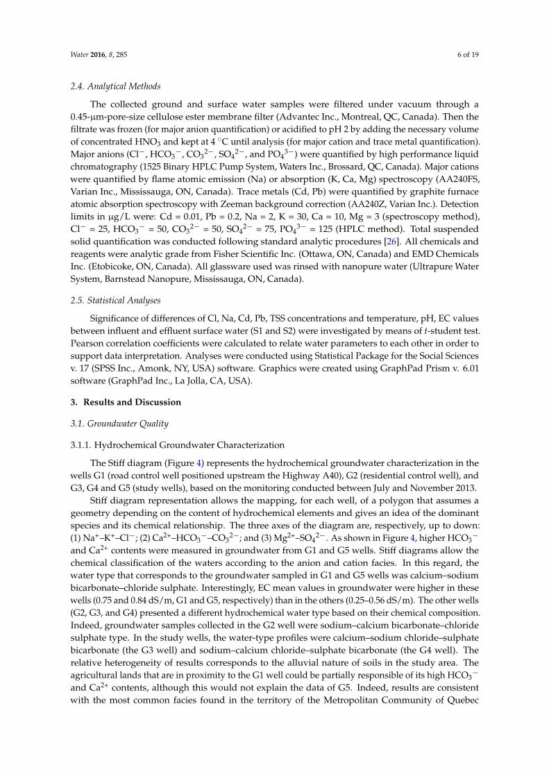
Figure 3. Pictures of the pilot site located in Saint‐Augustin Lake watershed (Quebec): (a) active
filtering bed entrance sump; (b) detention basin; (c) adapted constructed wetland—deep zone; and
(d) adapted constructed wetland—shallow zone.
The active filtering bed uses an underground reactive media composed of a limestone (80%) and
dolomite (20%) mixture. The functioning is based on the runoff circulating through a granular bed
(the reactive media) whose chemical properties enhance contaminant retention. Clean stone from the
reactive media has an average diameter between 5 mm and 10 mm, which could ensure a
permeability of 10 cm/s. The active filtering bed is 27 m long and 4.8 m wide (average width of the
trapezoid), which gives a flow section of 2.88 m2. The active filtering bed is totally isolated from both
soil and surface by an impermeable geotextile, and also from the base by the superposition of
granular material and a geomembrane.
The adapted constructed wetland is a free surface‐flow system where substrate, water and plants
imitate the processes occurring in natural swamps. The adapted constructed wetland consists of a
shallow pond divided into 3 plots of land where aquatic plants were cultivated. There is an inlet
control equipped with a drainage pipe and a valve at the outlet that controls the water level as needed
Figure 2. Surface water sampling points in the pilot site located in Saint-Augustin Lake watershed(Quebec). Red stars represent surface sampling points: S1 (influent water) and S2 (effluent water).
Water 2016, 8, 285 4 of 19
Figure 2. Surface water sampling points in the pilot site located in Saint‐Augustin Lake watershed
(Quebec). Red stars represent surface sampling points: S1 (influent water) and S2 (effluent water).
Figure 3. Pictures of the pilot site located in Saint‐Augustin Lake watershed (Quebec): (a) active
filtering bed entrance sump; (b) detention basin; (c) adapted constructed wetland—deep zone; and
(d) adapted constructed wetland—shallow zone.
The active filtering bed uses an underground reactive media composed of a limestone (80%) and
dolomite (20%) mixture. The functioning is based on the runoff circulating through a granular bed
(the reactive media) whose chemical properties enhance contaminant retention. Clean stone from the
reactive media has an average diameter between 5 mm and 10 mm, which could ensure a
permeability of 10 cm/s. The active filtering bed is 27 m long and 4.8 m wide (average width of the
trapezoid), which gives a flow section of 2.88 m2. The active filtering bed is totally isolated from both
soil and surface by an impermeable geotextile, and also from the base by the superposition of
granular material and a geomembrane.
The adapted constructed wetland is a free surface‐flow system where substrate, water and plants
imitate the processes occurring in natural swamps. The adapted constructed wetland consists of a
shallow pond divided into 3 plots of land where aquatic plants were cultivated. There is an inlet
control equipped with a drainage pipe and a valve at the outlet that controls the water level as needed
Figure 3. Pictures of the pilot site located in Saint-Augustin Lake watershed (Quebec): (a) active filteringbed entrance sump; (b) detention basin; (c) adapted constructed wetland—deep zone; and (d) adaptedconstructed wetland—shallow zone.
The active filtering bed uses an underground reactive media composed of a limestone (80%) anddolomite (20%) mixture. The functioning is based on the runoff circulating through a granular bed(the reactive media) whose chemical properties enhance contaminant retention. Clean stone from thereactive media has an average diameter between 5 mm and 10 mm, which could ensure a permeabilityof 10 cm/s. The active filtering bed is 27 m long and 4.8 m wide (average width of the trapezoid),which gives a flow section of 2.88 m2. The active filtering bed is totally isolated from both soil andsurface by an impermeable geotextile, and also from the base by the superposition of granular materialand a geomembrane.
The adapted constructed wetland is a free surface-flow system where substrate, water and plantsimitate the processes occurring in natural swamps. The adapted constructed wetland consists of ashallow pond divided into 3 plots of land where aquatic plants were cultivated. There is an inletcontrol equipped with a drainage pipe and a valve at the outlet that controls the water level as needed

Water 2016, 8, 285 5 of 19
by the plants. The adapted constructed wetland dimensions are: 850 m3 volume and 5/1 length/width.The bottom is impermeable, made from a bentonite geomembrane. Planted were typical wetlandplants, such as Typha angustifolia and Eleocharis palustris. Moreover, halophyte plants were planted, suchas Atriplex patula, Spergularia canadensis, and Salicornia europaea. Halophyte plants are an interestingalternative to plants traditionally used to treat the road effluents: (i) they are resistant to strong salinity;(ii) they can accumulate moderate to high quantities of salt in its biomass; and (iii) they can reduce theload of trace metals by bioaccumulation and biostabilisation [9,24].
2.3. Sampling Strategy
2.3.1. Groundwater
A strategic sampling has been set up to characterize and monitor groundwater based on thelocation of the A40 highway, the rainwater drainage, and the piezometric and well network installedin the study area. Indeed, several sampling wells and piezometers are installed in the Saint-AugustinLake watershed as part of previous research studies [20,25]. Based on these studies, several wells tocollect groundwater samples were selected (Figure 1): piezometer G1 (road control); monitoring wellG2 (residential control); and monitoring wells G3, G4, and G5 (study wells). Special attention wasplaced on the geological composition and land use of sites where selected wells are installed were assimilar and comparable as possible. The piezometer G1 is located upstream of the Highway A40. Inthis area groundwater is not affected by runoff pollution from Highway A40. The G2 groundwater wellis located in a residential area but away from the road area. In this area, groundwater is not affectedby runoff pollution but by residences. Therefore, G1 and G2 are considered as reference monitoringpoints not affected by road de-icing salts due to its location. In contrast, the G3 to G5 groundwaterwells are located upstream of Saint-Augustin Lake and placed in a North-West/South-East axis, beingaffected by both road and residential areas. Groundwater samples in duplicate were taken, with asingle valve bailer, once a week from July to November 2013 (135 days) in order to monitor Cl and Naconcentrations. Other major cations and anions (K+, Ca2+, Mg2+, HCO3
´, CO32´, SO4
2´, and PO43´),
as well as trace metals (Cd and Pb), were also monitored in this period. Some water quality indicators(temperature, pH, and electrical conductivity (EC)) were measured in situ using a multiprobe meter(Model YSI 6600 V2, YSI Inc., Yellow Springs, OH, USA). Water level was measured with an electricalprobe called “Deep water level”.
2.3.2. Surface Water
Surface water was sampled and monitored in all cases at two points at the pilot site (Figure 2).The first sampling point (S1) is located in a Highway A40 ditch at the entrance of the pilot sitecorresponding to influent water. The second sampling point (S2) is located at the exit of the pilot sitecorresponding to treated water or effluent water. Pilot site construction and plantation were finishedduring summer 2011. Between July and October 2011 some water quality indicators were measured insitu (temperature, pH, and EC) or in the laboratory (total suspended solids (TSS)). Then, the systemwas allowed to stabilize until spring 2012 (snow-melting period), when the monitoring was conducted.Surface water samples were taken once a week from March to November 2012 (238 days) in order tomonitor Cl and Na concentrations, water quality indicators (temperature, pH, EC, and TSS), as well astrace metal concentrations (Cd and Pb). Removal efficiency (%) of Na, Cl, Cd, and Pb was calculated interms of concentration by the following Equation (1):
Removal e f f iciency “Cin ´ Cout
Cinˆ 100 (1)
where Cin and Cout are the average influent and effluent concentrations, respectively, of Na, Cl, Cd, orPb (mg/L).
Water 2016, 8, 285 6 of 19
2.4. Analytical Methods
The collected ground and surface water samples were filtered under vacuum through a0.45-µm-pore-size cellulose ester membrane filter (Advantec Inc., Montreal, QC, Canada). Then thefiltrate was frozen (for major anion quantification) or acidified to pH 2 by adding the necessary volumeof concentrated HNO3 and kept at 4 ˝C until analysis (for major cation and trace metal quantification).Major anions (Cl´, HCO3
´, CO32´, SO4
2´, and PO43´) were quantified by high performance liquid
chromatography (1525 Binary HPLC Pump System, Waters Inc., Brossard, QC, Canada). Major cationswere quantified by flame atomic emission (Na) or absorption (K, Ca, Mg) spectroscopy (AA240FS,Varian Inc., Mississauga, ON, Canada). Trace metals (Cd, Pb) were quantified by graphite furnaceatomic absorption spectroscopy with Zeeman background correction (AA240Z, Varian Inc.). Detectionlimits in µg/L were: Cd = 0.01, Pb = 0.2, Na = 2, K = 30, Ca = 10, Mg = 3 (spectroscopy method),Cl´ = 25, HCO3
´ = 50, CO32´ = 50, SO4
2´ = 75, PO43´ = 125 (HPLC method). Total suspended
solid quantification was conducted following standard analytic procedures [26]. All chemicals andreagents were analytic grade from Fisher Scientific Inc. (Ottawa, ON, Canada) and EMD ChemicalsInc. (Etobicoke, ON, Canada). All glassware used was rinsed with nanopure water (Ultrapure WaterSystem, Barnstead Nanopure, Mississauga, ON, Canada).
2.5. Statistical Analyses
Significance of differences of Cl, Na, Cd, Pb, TSS concentrations and temperature, pH, EC valuesbetween influent and effluent surface water (S1 and S2) were investigated by means of t-student test.Pearson correlation coefficients were calculated to relate water parameters to each other in order tosupport data interpretation. Analyses were conducted using Statistical Package for the Social Sciencesv. 17 (SPSS Inc., Amonk, NY, USA) software. Graphics were created using GraphPad Prism v. 6.01software (GraphPad Inc., La Jolla, CA, USA).
3. Results and Discussion
3.1. Groundwater Quality
3.1.1. Hydrochemical Groundwater Characterization
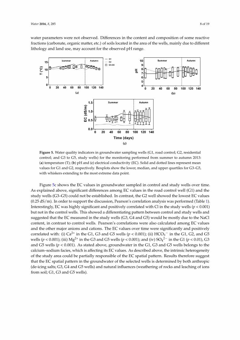
The Stiff diagram (Figure 4) represents the hydrochemical groundwater characterization in thewells G1 (road control well positioned upstream the Highway A40), G2 (residential control well), andG3, G4 and G5 (study wells), based on the monitoring conducted between July and November 2013.
Stiff diagram representation allows the mapping, for each well, of a polygon that assumes ageometry depending on the content of hydrochemical elements and gives an idea of the dominantspecies and its chemical relationship. The three axes of the diagram are, respectively, up to down:(1) Na+–K+–Cl´; (2) Ca2+–HCO3
´–CO32´; and (3) Mg2+–SO4
2´. As shown in Figure 4, higher HCO3´
and Ca2+ contents were measured in groundwater from G1 and G5 wells. Stiff diagrams allow thechemical classification of the waters according to the anion and cation facies. In this regard, thewater type that corresponds to the groundwater sampled in G1 and G5 wells was calcium–sodiumbicarbonate–chloride sulphate. Interestingly, EC mean values in groundwater were higher in thesewells (0.75 and 0.84 dS/m, G1 and G5, respectively) than in the others (0.25–0.56 dS/m). The other wells(G2, G3, and G4) presented a different hydrochemical water type based on their chemical composition.Indeed, groundwater samples collected in the G2 well were sodium–calcium bicarbonate–chloridesulphate type. In the study wells, the water-type profiles were calcium–sodium chloride–sulphatebicarbonate (the G3 well) and sodium–calcium chloride–sulphate bicarbonate (the G4 well). Therelative heterogeneity of results corresponds to the alluvial nature of soils in the study area. Theagricultural lands that are in proximity to the G1 well could be partially responsible of its high HCO3
´
and Ca2+ contents, although this would not explain the data of G5. Indeed, results are consistentwith the most common facies found in the territory of the Metropolitan Community of Quebec

Water 2016, 8, 285 7 of 19
City (Ca2+–HCO3´ and Na+–Cl´, associated with recharge areas), and show the typical intrinsic
heterogeneity in the spatial distribution of geological deposits of glaciofluvial origin [27]. Thesefacies are found almost exclusively on the north shore of the St. Lawrence River, in the St. LawrencePlatform formation.Water 2016, 8, 285 7 of 19
Figure 4. Stiff diagram of the groundwater of sampling wells (G1, road control; G2, residential control;
and G3 to G5, study wells). For each ion, data are expressed as mean values (meq/L) of the monitoring
performed from summer to autumn 2013. EC: electrical conductivity.
Overall, the groundwater sampled in the study wells (G3 to G5) is much more loaded in Cl than
in G1 and G2 control wells: 54% (G3), 67% (G4), and 42% (G5) of the sum of ions. As discussed below,
results suggest that the road runoff loaded with Cl from de‐icing salts leached into the soil and
reached the groundwater downstream of the road network. In contrast, Na was not always the
predominant cation in the study wells. This is probably because of Na ions are more easily retained
in soils than Cl ions and, therefore, lower Na concentrations in groundwater are expected. If we
consider the predominant ions: HCO3− was the predominant anion (>50% of the sum of anions) in
groundwater in G1, G2, and G5 wells, and Cl in G3 and G4 wells. Considering the cations, Ca was
predominant in G1, G3, and G5 wells, but Na in G2 and G4 wells.
Within the groundwater characterization, trace metal (Cd and Pb) concentration was also
monitored. However, Cd and Pb concentrations were in all cases below the detection limit.
3.1.2. Water Quality Indicators
Groundwater quality indicators (temperature, pH and EC) in G1, G2, G3, G4 and G5 wells were
monitored during summer and autumn seasons and are presented in Figure 5.
The groundwater temperatures ranged from 10 °C to 13 °C (Figure 5a). An increase in
groundwater temperature was observed during the summer period, with a decrease in autumn. The
highest temperatures were measured in the G1 well, road control (during the summer period), and
the smallest values in the G2 well, residential control. The temperatures in groundwater in the G3 to
G5 wells were intermediaries.
Regarding pH (Figure 5b), no clear temporal variation pattern was observed. Values fluctuated
from 5.6 to 8.3 in the G3 to G5 wells. In the case of control wells, the pH values in G1 were neutral
(around 7) while pHs tended to basicity in the G2 with values ≥ 8. The lowest pH values were
measured in the G4 and G5 study wells. Relationships between the pH values and the other measured
water parameters were not observed. Differences in the content and composition of some reactive
fractions (carbonate, organic matter, etc.) of soils located in the area of the wells, mainly due to
different lithology and land use, may account for the observed pH range.
Figure 4. Stiff diagram of the groundwater of sampling wells (G1, road control; G2, residential control;and G3 to G5, study wells). For each ion, data are expressed as mean values (meq/L) of the monitoringperformed from summer to autumn 2013. EC: electrical conductivity.
Overall, the groundwater sampled in the study wells (G3 to G5) is much more loaded in Cl thanin G1 and G2 control wells: 54% (G3), 67% (G4), and 42% (G5) of the sum of ions. As discussed below,results suggest that the road runoff loaded with Cl from de-icing salts leached into the soil and reachedthe groundwater downstream of the road network. In contrast, Na was not always the predominantcation in the study wells. This is probably because of Na ions are more easily retained in soils thanCl ions and, therefore, lower Na concentrations in groundwater are expected. If we consider thepredominant ions: HCO3
´ was the predominant anion (>50% of the sum of anions) in groundwater inG1, G2, and G5 wells, and Cl in G3 and G4 wells. Considering the cations, Ca was predominant in G1,G3, and G5 wells, but Na in G2 and G4 wells.
Within the groundwater characterization, trace metal (Cd and Pb) concentration was alsomonitored. However, Cd and Pb concentrations were in all cases below the detection limit.
3.1.2. Water Quality Indicators
Groundwater quality indicators (temperature, pH and EC) in G1, G2, G3, G4 and G5 wells weremonitored during summer and autumn seasons and are presented in Figure 5.
The groundwater temperatures ranged from 10 ˝C to 13 ˝C (Figure 5a). An increase ingroundwater temperature was observed during the summer period, with a decrease in autumn.The highest temperatures were measured in the G1 well, road control (during the summer period),and the smallest values in the G2 well, residential control. The temperatures in groundwater in the G3to G5 wells were intermediaries.
Regarding pH (Figure 5b), no clear temporal variation pattern was observed. Values fluctuatedfrom 5.6 to 8.3 in the G3 to G5 wells. In the case of control wells, the pH values in G1 were neutral(around 7) while pHs tended to basicity in the G2 with values ě 8. The lowest pH values weremeasured in the G4 and G5 study wells. Relationships between the pH values and the other measured
Water 2016, 8, 285 8 of 19
water parameters were not observed. Differences in the content and composition of some reactivefractions (carbonate, organic matter, etc.) of soils located in the area of the wells, mainly due to differentlithology and land use, may account for the observed pH range.Water 2016, 8, 285 8 of 19
Figure 5. Water quality indicators in groundwater sampling wells (G1, road control; G2, residential
control; and G3 to G5, study wells) for the monitoring performed from summer to autumn 2013: (a)
temperature (T); (b) pH and (c) electrical conductivity (EC). Solid and dotted lines represent mean
values for G1 and G2, respectively. Boxplots show the lower, median, and upper quartiles for G3–G5,
with whiskers extending to the most extreme data point.
Figure 5c shows the EC values in groundwater sampled in control and study wells over time.
As explained above, significant differences among EC values in the road control well (G1) and the
study wells (G3–G5) could not be established. In contrast, the G2 well showed the lowest EC values
(0.25 dS/m). In order to support the discussion, Pearson’s correlation analysis was performed (Table
1). Interestingly, EC was highly significant and positively correlated with Cl in the study wells
(p < 0.001) but not in the control wells. This showed a differentiating pattern between control and
study wells and suggested that the EC measured in the study wells (G3, G4 and G5) would be mostly
due to the NaCl content, in contrast to control wells. Pearson’s correlations were also calculated
among EC values and the other major anions and cations. The EC values over time were significantly
and positively correlated with: (i) Ca2+ in the G1, G3 and G5 wells (p < 0.001); (ii) HCO3− in the G1, G2,
and G5 wells (p < 0.001); (iii) Mg2+ in the G3 and G5 wells (p < 0.001); and (iv) SO42− in the G1 (p < 0.01),
G3 and G5 wells (p < 0.001). As stated above, groundwater in the G1, G3 and G5 wells belongs to the
calcium–sodium facies, which is affecting its EC values. As described above, the intrinsic
heterogeneity of the study area could be partially responsible of the EC spatial pattern. Results
therefore suggest that the EC spatial pattern in the groundwater of the selected wells is determined
by both anthropic (de‐icing salts; G3, G4 and G5 wells) and natural influences (weathering of rocks
and leaching of ions from soil; G1, G3 and G5 wells).
Figure 5. Water quality indicators in groundwater sampling wells (G1, road control; G2, residentialcontrol; and G3 to G5, study wells) for the monitoring performed from summer to autumn 2013:(a) temperature (T); (b) pH and (c) electrical conductivity (EC). Solid and dotted lines represent meanvalues for G1 and G2, respectively. Boxplots show the lower, median, and upper quartiles for G3–G5,with whiskers extending to the most extreme data point.
Figure 5c shows the EC values in groundwater sampled in control and study wells over time.As explained above, significant differences among EC values in the road control well (G1) and thestudy wells (G3–G5) could not be established. In contrast, the G2 well showed the lowest EC values(0.25 dS/m). In order to support the discussion, Pearson’s correlation analysis was performed (Table 1).Interestingly, EC was highly significant and positively correlated with Cl in the study wells (p < 0.001)but not in the control wells. This showed a differentiating pattern between control and study wells andsuggested that the EC measured in the study wells (G3, G4 and G5) would be mostly due to the NaClcontent, in contrast to control wells. Pearson’s correlations were also calculated among EC valuesand the other major anions and cations. The EC values over time were significantly and positivelycorrelated with: (i) Ca2+ in the G1, G3 and G5 wells (p < 0.001); (ii) HCO3
´ in the G1, G2, and G5wells (p < 0.001); (iii) Mg2+ in the G3 and G5 wells (p < 0.001); and (iv) SO4
2´ in the G1 (p < 0.01), G3and G5 wells (p < 0.001). As stated above, groundwater in the G1, G3 and G5 wells belongs to thecalcium–sodium facies, which is affecting its EC values. As described above, the intrinsic heterogeneityof the study area could be partially responsible of the EC spatial pattern. Results therefore suggestthat the EC spatial pattern in the groundwater of the selected wells is determined by both anthropic(de-icing salts; G3, G4 and G5 wells) and natural influences (weathering of rocks and leaching of ionsfrom soil; G1, G3 and G5 wells).

Water 2016, 8, 285 9 of 19
Table 1. Pearson’s correlation coefficients among groundwater parameters at each well.
Well Parameters T pH EC WL Cl´ Na+ Ca2+ Mg2+ K+ HCO3´ SO4
2´
G1
T 1 0.674 ** 0.788 *** 0.611 * ´0.458 ´0.252 0.696 ** 0.506 0.588 * 0.813 *** 0.472pH 1 0.549 * 0.234 ´0.395 ´0.192 0.553 * 0.458 0.251 0.368 0.416EC 1 0.368 ´0.514 * ´0.224 0.968 *** 0.366 0.708 ** 0.879 *** 0.660 **WL 1 0.075 0.057 0.176 0.680 ** 0.568 * 0.535 * 0.067Cl´ 1 0.547 * ´0.544 * ´0.398 ´0.252 ´0.437 ´0.438Na+ 1 ´0.321 ´0.344 0.056 ´0.336 0.092
G2
T 1 0.309 ´0.220 0.167 0.021 ´0.367 ´0.105 ´0.247 ´0.260 ´0.122 0.330pH 1 ´0.593 * 0.474 0.413 ´0.146 ´0.503 ´0.672 ** ´0.207 ´0.593 * ´0.145EC 1 ´0.109 0.232 0.335 0.532 * 0.520 * 0.356 0.930 *** ´0.157WL 1 0.506 ´0.162 ´0.201 ´0.168 0.350 ´0.137 ´0.009Cl´ 1 0.307 ´0.269 ´0.150 0.258 0.063 ´0.085Na+ 1 ´0.048 0.230 0.311 0.014 0.024
G3
T 1 ´0.270 0.472 0.554 * 0.563 * 0.148 0.392 0.400 ´0.440 ´0.198 0.283pH 1 ´0.876 *** ´0.727 ** ´0.903 *** ´0.442 ´0.871 *** ´0.725 ** 0.100 0.350 ´0.905 ***EC 1 0.808 *** 0.951 *** 0.405 0.968 *** 0.889 *** ´0.201 ´0.076 0.916 ***WL 1 0.822 *** 0.337 0.769 ** 0.668 ** ´0.087 ´0.226 0.778 **Cl´ 1 0.508 0.889 *** 0.754 ** ´0.288 ´0.293 0.872 ***Na+ 1 0.304 0.143 ´0.089 ´0.518 * 0.466
G4
T 1 ´0.259 ´0.349 0.334 ´0.323 ´0.133 ´0.499 ´0.185 0.378 ´0.328 0.412pH 1 0.615 * 0.618 * 0.605 * 0.542 * 0.399 0.283 ´0.238 0.258 ´0.446EC 1 0.280 0.787 *** 0.881 *** 0.495 0.447 ´0.219 0.591 * ´0.510WL 1 0.251 0.387 0.035 0.366 0.046 0.035 ´0.438Cl´ 1 0.551 * 0.367 0.458 ´0.466 0.120 ´0.342Na+ 1 0.295 0.534 * ´0.109 0.469 ´0.530 *
G5
T 1 0.059 0.287 0.454 0.287 0.156 0.302 0.255 0.138 0.233 0.238pH 1 ´0.661 ** ´0.600 * ´0.694 ** ´0.510 ´0.660 ** ´0.681 ** 0.059 ´0.528 * ´0.689 **EC 1 0.946 *** 0.973 *** 0.818 *** 0.989 *** 0.950 *** 0.295 0.937 *** 0.978 ***WL 1 0.941 *** 0.704 ** 0.930 *** 0.905 *** 0.145 0.897 *** 0.886 ***Cl´ 1 0.751 ** 0.944 *** 0.952 *** 0.276 0.888 *** 0.952 ***Na+ 1 0.788 *** 0.777 ** 0.318 0.700 ** 0.833 ***
Notes: T: Temperature; EC: Electrical conductivity; WT: Water level. * p < 0.05; ** p < 0.01; *** p < 0.001, statistical significance at these probability levels (n = 15).

Water 2016, 8, 285 10 of 19
Regarding the temporal pattern, although mean EC values in control wells remained almostconstant throughout the study period (0.68–0.89 dS/m in G1 and 0.21–0.29 dS/m in G2), a differentpattern was observed in the study wells (G3, G4 and G5). Thus, the range of variation is much largerin autumn (linked with more precipitation) than in summer. When the EC values in groundwater areevaluated separately taking into account each of the study wells, it was observed that EC: decreases(from 0.64 to 0.36 dS/m in G3), is almost constant (from 0.53 to 0.63 dS/m in G4), or increases (from0.58 to 1.17 dS/m in G5) over time. Results were compared to the water levels measured at each wellover time (data not shown). Pearson correlation analysis showed significant and positive correlationsbetween EC values and the water level in the G3 and G5 wells (p < 0.001) (Table 1). Results thereforeshowed that the higher the water level, the higher the EC in groundwater and that this pattern wasnot apparently seasonally dependent. Nonetheless, the longer residence time of groundwater thanthat of surface water could be offsetting the seasonal pattern. Higher infiltration of water charged insalts during the increase of water levels may account for the positive correlation obtained between theEC values and the water level, which deserves further studies.
3.1.3. NaCl Concentration
The concentration of Cl and Na in groundwater (G1 to G5 wells) has been monitored from summerto autumn 2013 (Figure 6).
Water 2016, 8, 285 10 of 19
Regarding the temporal pattern, although mean EC values in control wells remained almost
constant throughout the study period (0.68–0.89 dS/m in G1 and 0.21–0.29 dS/m in G2), a different
pattern was observed in the study wells (G3, G4 and G5). Thus, the range of variation is much larger
in autumn (linked with more precipitation) than in summer. When the EC values in groundwater are
evaluated separately taking into account each of the study wells, it was observed that EC: decreases
(from 0.64 to 0.36 dS/m in G3), is almost constant (from 0.53 to 0.63 dS/m in G4), or increases (from
0.58 to 1.17 dS/m in G5) over time. Results were compared to the water levels measured at each well
over time (data not shown). Pearson correlation analysis showed significant and positive correlations
between EC values and the water level in the G3 and G5 wells (p < 0.001) (Table 1). Results therefore
showed that the higher the water level, the higher the EC in groundwater and that this pattern was
not apparently seasonally dependent. Nonetheless, the longer residence time of groundwater than
that of surface water could be offsetting the seasonal pattern. Higher infiltration of water charged in
salts during the increase of water levels may account for the positive correlation obtained between
the EC values and the water level, which deserves further studies.
3.1.3. NaCl Concentration
The concentration of Cl and Na in groundwater (G1 to G5 wells) has been monitored from
summer to autumn 2013 (Figure 6).
Figure 6. Concentration of Cl and Na in groundwater sampling wells (G1, road control; G2, residential
control; and G3 to G5, study wells) for the monitoring performed from summer to autumn 2013:
(a) Cl and (b) Na. Solid and dottedlines represent mean values for G1 and G2, respectively. Boxplots
show the lower, median, and upper quartiles for G3–G5, with whiskers extending to the most extreme
data point.
The Cl concentration in groundwater in the two control wells (4 and 22 mg/L in G1 and G2
respectively, ~13 mg/L on average) was in all cases lower than that quantified in the study wells (from
39 to 222 g/L, 125 mg/L on average, G3–G5). Interestingly, results showed that even though major ion
concentrations (Figure 4) and EC values (Figure 5) are elevated in G1 well, Na and Cl concentrations
are very low (Figure 6). The higher Cl concentrations obtained in G2 with respect to G1 can be
explained by the residential character of the area. Indeed, septic tanks are possible sources of
groundwater salinization [8]. The higher Cl concentration in groundwater in the study wells (G3 to
G5) than in the control wells (G1 and G2) indicates that the road network and de‐icing salts impact
the groundwater chemical composition. This observation was also stated by Daley et al. [8], which
reported that sewage and water softeners accounted for only 7% of the Na and Cl input to a single
Figure 6. Concentration of Cl and Na in groundwater sampling wells (G1, road control; G2, residentialcontrol; and G3 to G5, study wells) for the monitoring performed from summer to autumn 2013: (a) Cland (b) Na. Solid and dottedlines represent mean values for G1 and G2, respectively. Boxplots show thelower, median, and upper quartiles for G3–G5, with whiskers extending to the most extreme data point.
The Cl concentration in groundwater in the two control wells (4 and 22 mg/L in G1 and G2respectively, ~13 mg/L on average) was in all cases lower than that quantified in the study wells(from 39 to 222 g/L, 125 mg/L on average, G3–G5). Interestingly, results showed that even thoughmajor ion concentrations (Figure 4) and EC values (Figure 5) are elevated in G1 well, Na and Clconcentrations are very low (Figure 6). The higher Cl concentrations obtained in G2 with respect to G1can be explained by the residential character of the area. Indeed, septic tanks are possible sources ofgroundwater salinization [8]. The higher Cl concentration in groundwater in the study wells (G3 toG5) than in the control wells (G1 and G2) indicates that the road network and de-icing salts impactthe groundwater chemical composition. This observation was also stated by Daley et al. [8], whichreported that sewage and water softeners accounted for only 7% of the Na and Cl input to a single

Water 2016, 8, 285 11 of 19
rural watershed in New Hampshire, whereas NaCl used for de-icing accounted for 91%. RegardingNa, the same pattern was observed as in the case of Cl. Thus, Na concentration in groundwater inthe two control wells (G1 and G2) showed the lowest values (33 mg/L on average). In the case of thestudy wells (64 mg/L Na on average, G3–G5), the maximum Na values even reached up to 112 mg/L.This showed the importance of the Highway and road network on the contamination of groundwater.As it was observed for EC, the range of variability in Cl concentration in the study wells was higher inautumn than in summer, attributed to the cooler temperatures and higher precipitation rates duringautumn, which facilitates flushing of salts through groundwater. A relationship with the water levelwas also observed (Table 1). Thus, significant and positive correlations among the water level wereobtained with Cl in the G3 and G5 wells (p < 0.001) and with Na in the G5 well (p < 0.01). As statedabove, EC and Cl and Na ions were significantly positively correlated to each other in the study wells(p < 0.001) but not in the control wells. These results are in accordance with the study conducted byGalvez-Cloutier et al. [20] for the same lake and season.
Groundwater is an important source of drinking water. According to McConnell and Lewis [28],25% to 50% of road de-icing salt may reach groundwater, increasing the salinity of drinking watersources in public distribution networks. Data on drinking water from several Canadian provincesindicate that the Cl concentrations are generally less than 10 mg/L [29]. In the present study, resultsshowed that Cl concentrations in study wells (G3–G5) are very high, up to 22 times higher than10 mg/L. In the case of Na, the concentration ranges in both the control wells (28–30 mg/L Na) andthe study wells (37–112 mg/L Na) were within the normal ranges for groundwater in Canada (from6 to 130 mg/L) [30]. The concentrations of Cl and Na remained in all cases below the drinking waterquality standards of Canada: 250 mg/L and 200 mg/L, respectively [31]. However, results highlightthat the highest NaCl concentration is found in the groundwater from the areas of the watershedaffected by the road network (study wells), which makes it essential to perform long term monitoring.
3.2. Surface Water Quality
3.2.1. Water Quality Indicators
Table 2 shows the water quality indicators measured in influent (S1) and effluent (S2) surfacewater at the pilot site during summer and autumn, 2011, after its construction. During the first periodof operation (from mid-2011), no significant differences were observed on water quality indicatorsbetween S1 and S2 sampling points. Nonetheless, a trend to decrease was observed on EC (from1.9 dS/m at S1 to 1.1 dS/m at S2) with higher values during the summer period. A decreasing trendon the concentration of TSS was also observed, from 194.5 µg/L (S1) to 24.1 µg/L (S2), suggesting theretention of particles by the system.
Table 2. Water quality indicators (mean and range) measured in influent (S1) and effluent (S2) surfacewater in the pilot site after its construction, from late summer to autumn 2011.
ParametersInfluent (S1) Effluent (S2)
Units Min Max Mean SEM Min Max Mean SEM
T ˝C 9.1 17.5 14.1 1.8 8.9 19.2 16.3 2.5pH - 7.4 8.2 7.8 0.1 7.1 8.2 7.7 0.2EC dS/m 0.7 2.8 1.9 0.4 0.6 2.2 1.1 0.3TSS µg/L 2.2 386.8 194.5 192.3 12.4 35.8 24.1 11.7
Notes: SEM: Standard error of mean; T: Temperature; EC: Electrical conductivity; TSS: Total suspended solids.
A comprehensive monitoring was completed between March and November in 2012. Data onclimatic conditions (ambient temperature, and total precipitation) during this period are shown inFigure 7. Surface water quality indicators (water temperature, pH, EC, and TSS) in S1 and S2 samplingpoints along the performed monitoring are shown in Figure 8.

Water 2016, 8, 285 12 of 19Water 2016, 8, 285 12 of 19
Figure 7. Precipitation and temperature from spring to autumn 2012 (Station Jean Lesage, Quebec).
Figure 8. Water quality indicators in influent (S1) and effluent (S2) surface water along the monitoring
performed in the pilot site from spring to autumn 2012: (a) temperature (T); (b) pH; (c) electrical
conductivity (EC) and (d) total suspended solids (TSS).
Depending on the season, water temperature ranged from 8.6 °C (spring) to 26.2 °C (summer)
(Figure 8a), and was generally related to the ambient temperature (Figure 7) with no differences from
S1 to S2 sampling points. Water pH values were from neutral to moderately alkaline, between 6.9
and 8.3 (Figure 8b), suitable to permit the existence of most living organisms [32]. No pattern on pH
values according to the season was observed, and no differences between influent and effluent water
(S1 and S2). The values of EC in surface water (Figure 8c) were highly variable over time, as
previously reported for road runoff [5,33]. The EC values ranged from 0.5 to 5.4 dS/m (S1) and from
Figure 7. Precipitation and temperature from spring to autumn 2012 (Station Jean Lesage, Quebec).
Water 2016, 8, 285 12 of 19
Figure 7. Precipitation and temperature from spring to autumn 2012 (Station Jean Lesage, Quebec).
Figure 8. Water quality indicators in influent (S1) and effluent (S2) surface water along the monitoring
performed in the pilot site from spring to autumn 2012: (a) temperature (T); (b) pH; (c) electrical
conductivity (EC) and (d) total suspended solids (TSS).
Depending on the season, water temperature ranged from 8.6 °C (spring) to 26.2 °C (summer)
(Figure 8a), and was generally related to the ambient temperature (Figure 7) with no differences from
S1 to S2 sampling points. Water pH values were from neutral to moderately alkaline, between 6.9
and 8.3 (Figure 8b), suitable to permit the existence of most living organisms [32]. No pattern on pH
values according to the season was observed, and no differences between influent and effluent water
(S1 and S2). The values of EC in surface water (Figure 8c) were highly variable over time, as
previously reported for road runoff [5,33]. The EC values ranged from 0.5 to 5.4 dS/m (S1) and from
Figure 8. Water quality indicators in influent (S1) and effluent (S2) surface water along the monitoringperformed in the pilot site from spring to autumn 2012: (a) temperature (T); (b) pH; (c) electricalconductivity (EC) and (d) total suspended solids (TSS).
Depending on the season, water temperature ranged from 8.6 ˝C (spring) to 26.2 ˝C (summer)(Figure 8a), and was generally related to the ambient temperature (Figure 7) with no differencesfrom S1 to S2 sampling points. Water pH values were from neutral to moderately alkaline, between6.9 and 8.3 (Figure 8b), suitable to permit the existence of most living organisms [32]. No pattern onpH values according to the season was observed, and no differences between influent and effluentwater (S1 and S2). The values of EC in surface water (Figure 8c) were highly variable over time, aspreviously reported for road runoff [5,33]. The EC values ranged from 0.5 to 5.4 dS/m (S1) and from0.7 to 4.0 dS/m (S2), consistent with the data obtained by Galvez-Cloutier et al. [20] in road side ditchesat the same section of the Highway A40. In contrast to that observed for groundwater, in the case of

Water 2016, 8, 285 13 of 19
surface water, the highest EC values were measured in summer and the lowest in both autumn and theearly spring. Thus EC values in August and September (3.3–5.4 dS/m) were up to four times higherthan in April and May (0.8–2.4 dS/m). Low precipitation, associated with higher ambient temperature,increases salt concentration in water and hence EC. Indeed, this seasonal pattern observed on EC insurface water in both S1 and S2 points (Figure 8c) is consistent with the low total precipitation andhigh temperatures recorded from mid to late summer (Figure 7). In the fall, EC gradually declinedaccording to the lowest ambient temperature, reaching values similar to those of early spring. Electricalconductivity at S2 was 25% lower than at S1 during August and September, in accordance to thatobserved in 2011 (Table 2), thus suggesting salt removal by the system during this period.
Regarding particulate matter (Figure 8d), high fluctuations on TSS concentrations were observedin surface water in both S1 and S2 sampling points, with a range from 0.6 mg/L (minimum inS2) to 165.6 mg/L (maximum in S1). Values were low taking into account the traffic intensity ofHighway A40 [34] and when compared with the TSS concentration ranges reported for road runoffin other studies: 18–3165 mg/L [33], 13–4800 mg/L [35], and 1–5100 mg/L [2]. Regarding rainfall,a positive relation was observed among the peaks in TSS concentration (Figure 8d) and the peaksin total precipitation (Figure 7), but significant correlations could not be established (Table 3). Theconcentration of TSS in road runoff is dependent on a number of factors including storms events,rainfall intensity and duration, an antecedent dry weather period, wind, traffic volume and type,traffic during storms, watershed extension, land use in surrounding areas (residential, urban, andagricultural), TSS particle size, and so on [35–38]. The complexity of interactions among these factorsmay account for the lack of significant correlations between TSS concentration and the climatic data.When comparing the annual average concentration of TSS between S1 and S2 points, a slight overalldecrease was observed.
Table 3. Pearson’s correlation coefficients among influent (S1) and effluent (S2) surfacewater parameters.
SamplingPoints Parameters T pH EC TSS Cl Na Cd Pb
S1 vs. S1
T 1 0.224 0.169 0.292 0.221 0.308 0.481 ´0.069pH 1 ´0.230 0.149 0.002 ´0.063 0.059 ´0.293EC 1 0.153 0.787 *** 0.880 *** 0.606 ** 0.857 ***TSS 1 0.092 0.155 ´0.120 ´0.045Cl 1 0.922 *** 0.852 *** 0.611 *Na 1 0.766 *** 0.810 ***Cd 1 0.481Pb 1
S2 vs. S2
T 1 0.094 0.073 ´0.321 ´0.014 0.122 0.117 0.292pH 1 ´0.033 ´0.025 ´0.303 ´0.352 ´0.282 ´0.190EC 1 0.358 0.913 *** 0.914 *** 0.670 * 0.810 ***TSS 1 0.226 0.227 ´0.066 0.140Cl 1 0.908 *** 0.757 ** 0.701 **Na 1 0.775 *** 0.843 ***Cd 1 0.514Pb 1
S1 vs. S2
T 0.925 *** ´0.034 0.177 ´0.383 0.119 0.264 0.426 0.313pH 0.335 0.815 ** 0.108 0.046 ´0.223 ´0.201 0.005 ´0.083EC 0.026 ´0.349 0.898 *** 0.384 0.770 *** 0.843 *** 0.726 ** 0.807 ***TSS 0.372 ´0.077 0.118 0.376 0.059 0.233 ´0.081 0.189Cl 0.109 ´0.110 0.852 *** 0.329 0.850 *** 0.871 *** 0.869 *** 0.718 **Na 0.157 ´0.231 0.902 *** 0.277 0.859 *** 0.918 *** 0.862 *** 0.824 ***Cd 0.201 ´0.229 0.607 * ´0.188 0.698 ** 0.679 ** 0.914 *** 0.356Pb ´0.132 ´0.269 0.820 *** 0.222 0.755 ** 0.763 ** 0.699 * 0.846 ***
Notes: T: Temperature; EC: Electrical conductivity; TSS: total suspended solids. * p < 0.05; ** p < 0.01; *** p < 0.001,statistical significance at these probability levels (n = 26).

Water 2016, 8, 285 14 of 19
3.2.2. NaCl Concentration and Removal Efficiency
The concentration of Cl and Na in surface water (S1 and S2 points) along the monitoring performedin the pilot site from spring to autumn 2012 is shown in Figure 9.
Water 2016, 8, 285 14 of 19
The concentration of Cl and Na in surface water (S1 and S2 points) along the monitoring
performed in the pilot site from spring to autumn 2012 is shown in Figure 9.
Figure 9. Concentration of Cl and Na in influent (S1) and effluent (S2) surface water along the
monitoring performed in the pilot site from spring to autumn 2012: (a) Cl and (b) Na.
Overall, the Cl and Na concentrations measured in influent water (S1) were high and ranged
from 63 to 1757 mg/L Cl and from 61 to 846 mg/L Na. Values were in the same magnitude order as
the concentrations reported prior to the pilot site construction [20] which suggests that the amount
of de‐icing salts used on Highway A40 (and in the road network around the highway) during winter
road maintenance has not decreased in the last years. Data also revealed a salt pollution problem that
may impacts the ecosystem services provided by surface water in the watershed [6]. The extreme salt
concentration fluctuations (mostly in summer) can have severe impacts on the aquatic biota [5].
Indeed in 61% of influent water samples both Cl and Na concentrations exceeded the surface water
quality criteria established by Quebec Environment Ministry for the prevention of contamination in
water and aquatic organisms (250 mg/L Cl, 200 mg/L Na) [39]. Likewise, in 65% of samples, Cl
concentrations exceeded the US Environmental Protection Agency chronic effect standard (230 mg/L Cl)
and in 23% the acute exposure standard (860 mg/L Cl) for aquatic life in fresh water [40]. Data within
the ranges are often reported for road runoff: 17–10,400 mg/L Na [33], 1–298 mg/L Na and
1–573 mg/L Cl [8]. Nonetheless, the very high NaCl concentration fluctuations due to different site‐
specific and climatic conditions make comparability with other studies limited.
Positive and highly significant correlations (p < 0.001) between Cl and Na concentrations and EC
values were obtained (Table 3). Indeed, Cl and Na concentrations and EC values in surface water,
both in influent (S1) and effluent (S2), showed the same temporal pattern (Figures 8 and 9): increase
in the mid and late summer, then decrease in autumn. Seasonal NaCl concentration ranges (both S1
and S2) were as follows: 61–559 mg/L Na and 101–799 mg/L Cl (spring) < 114–846 mg/L Na and 158–
1757 mg/L Cl (summer) > 71–449 mg/L Na and 63–569 mg/L Cl (autumn). Higher NaCl concentrations
in winter during de‐icing salt applications [5,33] or in spring after snow‐melting [41] are often
expected. However, data from the present study showed a clear increase of NaCl concentration in
summer. The temporal pattern of NaCl concentration is linked to climatic conditions: the highest
Figure 9. Concentration of Cl and Na in influent (S1) and effluent (S2) surface water along themonitoring performed in the pilot site from spring to autumn 2012: (a) Cl and (b) Na.
Overall, the Cl and Na concentrations measured in influent water (S1) were high and rangedfrom 63 to 1757 mg/L Cl and from 61 to 846 mg/L Na. Values were in the same magnitude order asthe concentrations reported prior to the pilot site construction [20] which suggests that the amount ofde-icing salts used on Highway A40 (and in the road network around the highway) during winterroad maintenance has not decreased in the last years. Data also revealed a salt pollution problem thatmay impacts the ecosystem services provided by surface water in the watershed [6]. The extreme saltconcentration fluctuations (mostly in summer) can have severe impacts on the aquatic biota [5]. Indeedin 61% of influent water samples both Cl and Na concentrations exceeded the surface water qualitycriteria established by Quebec Environment Ministry for the prevention of contamination in water andaquatic organisms (250 mg/L Cl, 200 mg/L Na) [39]. Likewise, in 65% of samples, Cl concentrationsexceeded the US Environmental Protection Agency chronic effect standard (230 mg/L Cl) and in23% the acute exposure standard (860 mg/L Cl) for aquatic life in fresh water [40]. Data within theranges are often reported for road runoff: 17–10,400 mg/L Na [33], 1–298 mg/L Na and 1–573 mg/LCl [8]. Nonetheless, the very high NaCl concentration fluctuations due to different site-specific andclimatic conditions make comparability with other studies limited.
Positive and highly significant correlations (p < 0.001) between Cl and Na concentrations andEC values were obtained (Table 3). Indeed, Cl and Na concentrations and EC values in surface water,both in influent (S1) and effluent (S2), showed the same temporal pattern (Figures 8 and 9): increasein the mid and late summer, then decrease in autumn. Seasonal NaCl concentration ranges (bothS1 and S2) were as follows: 61–559 mg/L Na and 101–799 mg/L Cl (spring) < 114–846 mg/L Naand 158–1757 mg/L Cl (summer) > 71–449 mg/L Na and 63–569 mg/L Cl (autumn). Higher NaClconcentrations in winter during de-icing salt applications [5,33] or in spring after snow-melting [41] are

Water 2016, 8, 285 15 of 19
often expected. However, data from the present study showed a clear increase of NaCl concentrationin summer. The temporal pattern of NaCl concentration is linked to climatic conditions: thehighest concentrations of NaCl in water at higher temperature and lower precipitation, i.e., highertemperature/precipitation ratio, as occurs in summer [42]. Indeed, as discussed above for EC,evaporation processes occurring during summer involve a decrease in surface water flow and then anincrease in salt concentration in water. Therefore, our study suggests that high Cl and Na concentrationsmay be expected in the Saint-Augustin Lake watershed in summer. Chloride soluble concentrations insurface water were generally higher than Na concentrations (2–3 fold) (Figure 9). The Cl ions are verysoluble and less favourable to be adsorbed onto soil colloids than Na ions which can be adsorbed dueto cation exchange reactions by displacing cations such as Ca2+ and Mg2+ [42,43]. The different affinityof Cl and Na for particle sorption may account for the molar imbalance observed between Cl and Nain surface water.
The seasonal performance of the pilot site (including detention basin, active filtering bed,and adapted constructed wetland units) was evaluated by calculating the Cl and Na removalefficiency considering the concentration difference between influent (S1) and effluent (S2) surfacewater (Equation (1)). The seasonal removal efficiency was as follows: 16% Cl and 10.6% Na (spring),18.1% Cl and 24.5% Na (summer), and 19.7% Cl and 3% Na (autumn). Data corresponds to thefirst year of operation (2012). Higher performance is expected in the subsequent years with thematuration of the system due to growth and development of vegetation and the increase of micro- andmacroorganism biomass and activity, as previously reported in adapted constructed wetland undercold climate [44]. Data showed a different removal pattern depending on the element, Cl or Na. ThusCl removal remained almost constant over the pilot site operational period. However, in the case ofNa, the performance of the system was higher during summer, followed by spring, which deservesfurther studies.
3.2.3. Trace Metal Concentration and Removal Efficiency
The concentration of dissolved Cd and Pb in surface water (S1 and S2 points) along the monitoringperformed from spring to summer 2012 is shown in Figure 10.
Water 2016, 8, 285 15 of 19
concentrations of NaCl in water at higher temperature and lower precipitation, i.e., higher
temperature/precipitation ratio, as occurs in summer [42]. Indeed, as discussed above for EC,
evaporation processes occurring during summer involve a decrease in surface water flow and then
an increase in salt concentration in water. Therefore, our study suggests that high Cl and Na
concentrations may be expected in the Saint‐Augustin Lake watershed in summer. Chloride soluble
concentrations in surface water were generally higher than Na concentrations (2–3 fold) (Figure 9).
The Cl ions are very soluble and less favourable to be adsorbed onto soil colloids than Na ions which
can be adsorbed due to cation exchange reactions by displacing cations such as Ca2+ and Mg2+ [42,43].
The different affinity of Cl and Na for particle sorption may account for the molar imbalance observed
between Cl and Na in surface water.
The seasonal performance of the pilot site (including detention basin, active filtering bed, and
adapted constructed wetland units) was evaluated by calculating the Cl and Na removal efficiency
considering the concentration difference between influent (S1) and effluent (S2) surface water
(Equation (1)). The seasonal removal efficiency was as follows: 16% Cl and 10.6% Na (spring), 18.1%
Cl and 24.5% Na (summer), and 19.7% Cl and 3% Na (autumn). Data corresponds to the first year of
operation (2012). Higher performance is expected in the subsequent years with the maturation of the
system due to growth and development of vegetation and the increase of micro‐ and macroorganism
biomass and activity, as previously reported in adapted constructed wetland under cold climate [44].
Data showed a different removal pattern depending on the element, Cl or Na. Thus Cl removal
remained almost constant over the pilot site operational period. However, in the case of Na,
the performance of the system was higher during summer, followed by spring, which deserves
further studies.
3.2.3. Trace Metal Concentration and Removal Efficiency
The concentration of dissolved Cd and Pb in surface water (S1 and S2 points) along the
monitoring performed from spring to summer 2012 is shown in Figure 10.
Figure 10. Concentration of trace metals in influent (S1) and effluent (S2) surface water along the
monitoring performed in the pilot site from spring to summer 2012: (a) Cd and (b) Pb. Figure 10. Concentration of trace metals in influent (S1) and effluent (S2) surface water along themonitoring performed in the pilot site from spring to summer 2012: (a) Cd and (b) Pb.

Water 2016, 8, 285 16 of 19
Cadmium and Pb concentration in autumn was not presented because it was below detection limit.Trace metal concentration in both S1 and S2 points ranged as follows: 0.2–3.2 µg/L Cd (0.98 µg/L mean)and 0.3–67.8 µg/L Pb (16.6 µg/L mean). In all cases, Cd concentration was under the surface waterquality criteria established by the Quebec Environment Ministry for the prevention of contamination inwater and aquatic organisms (5 µg/L Cd) [39]. In contrast, in 56% of water samples, Pb concentrationsexceeded the same quality criteria (10 µg/L Pb). However, according to USEPA [40], in 97% (Cd) and71% (Pb) of water samples the chronic effect standard for aquatic life in fresh water (0.25 µg/L Cdand 2.5 µg/L Pb) was exceeded, as well as in 15% (Cd) and 3% (Pb) of the acute exposure standard(2 µg/L Cd and 65 µg/L Pb). The ranges of Cd and Pb concentration quantified in the present studywere expectedly high because of the high daily traffic density in the Highway A40. High metalconcentrations can also be related to the high amount of de-icing salts spread [45,46] and the increasedtear, wear, and corrosion due to the application of gravel at cold weather conditions [33]. Values are inline with those reported in other studies in road runoff: 0.02–6.1 µg/L dissolved Cd (0.2 µg/L mean)and 0.2–414 µg/L dissolved Pb (5.4 µg/L mean) in urban and non-urban highways [2]; 1.5–72.3 µg/Ltotal Pb in urban highways during storm events [47]; 400 µg/L event mean Pb concentration inhighways with >30,000 vehicles/day [48].
Significant positive correlations among Cd, Pb, Na, and Cl concentrations were obtained(p < 0.001 Cd and Pb vs. Na, p < 0.01 Cd and Pb vs. Cl) (Table 3). Indeed, temporal patternsin Cd, Pb, Na, and Cl concentrations in surface water (both in S1 and S2) were similar: increasefrom mid to late summer, then a decrease in autumn (Figures 9 and 10). As discussed above, thehigher temperature/precipitation ratio occurring in summer can explain this result (Figure 7). Thepositive correlations may also be related to metal mobilization processes by the formation of metallicchlorocomplexes, favoured at pHs of the present study [41,49]. In this regard, Bäckström et al. [11]studied the seasonal variations of trace metals in soil solution as a function of the distance from theroad in Sweden. They observed that the dominant speciation of Cd and Pb at 4 m from the road was:(i) Cd2+, CdCl+ and CdCl2 (for Cd); and (ii) Pb2+, PbCl+ and PbCO3 (for Pb). In road runoff, particulatematter is considered as one of the major pollutants since many pollutants are attached to it and washedoff [37]. In the present study, significant Pearson correlations between Cd and Pb concentrationsand TSS were not found (nor between TSS and Cl and Na), even taking into account each seasonseparately (Table 3). Despite Cd and Pb in road runoff are often associated with suspended solids, Cdand Pb adsorption can be far different depending on the fraction sizes, peaking at the fine particles(<40 µm) [48]. In this regard, climatic conditions could play an important role. Westerlund et al. [50]observed that metals during snow-melting were more particulate bound than during the rainy periodswith a higher percentage of the dissolved fraction. Nevertheless, at low ambient temperature theaccumulation of metals in particles decreases [49]. Further studies considering the seasonal pattern ofTSS particle size and trace metal distribution could be of great interest.
The seasonal performance of the pilot site was evaluated by Cd and Pb removal efficiency(Equation (1)). The seasonal removal efficiency in the first year of operation was as follows: 10.3% Cdand 6.8% Pb (spring), and ´6.7% Cd and 35.8% Pb (summer). As for NaCl, higher performance isexpected in the subsequent years. The negative removal rate of Cd in summer could be the result ofpollutants entering the pilot site outlet, considering its proximity to the Highway A40 [34,47].
4. Conclusions
From this research project, conclusions about the groundwater and surface water monitoringconducted in the Saint-Augustin Lake watershed can be established. The concentrations of Cl andNa in groundwater were higher in study wells (affected by road network) than in control wells. Ourfindings suggest therefore that de-icing salts spread in the watershed roads impact the groundwaterchemical composition. Regarding surface water, the pilot site (composed of a detention basin, anactive filtering bed and an adapted constructed wetland) has been proposed as a solution to reducethe concentrations of NaCl, as well as trace metals (Cd and Pb), at a watershed scale. Monitoring of

Water 2016, 8, 285 17 of 19
water surface showed that both NaCl concentrations and EC values follow a seasonal dependence.Thus, NaCl concentrations and EC values increased in mid and late summer (linked with the lowestprecipitation and highest temperature recorded), and then decrease in autumn. The removal efficiencyof Na by the pilot site was also dependent of the season, being the highest in summer, but constant inthe case of Cl. Cadmium and Pb concentrations were consistent with the traffic density and followeda similar temporal pattern to that observed for NaCl and EC. The highest Pb removal was found insummer. The pilot site has shown to be a useful strategy to mitigate the impact of anthropogenicsalinity at watershed scale, although it would take a few years of operation to observe its optimalperformance. It should also be considered that the data are limited as an aggregate comparison ofupstream/downstream of the pilot site, which is comprised of three units. This study deserves to bepursued and taken further in order to complete the data and to determine long-term conclusions.
Acknowledgments: The authors especially wish to thank Luke Pettet for English revisions. We thank the editorand the anonymous referees for helpful suggestions.
Author Contributions: Rosa Galvez conceived and designed the experiments; Hamdi Messaoud, Arthur Michauxand Samuel Roy performed the experiments; Gaëlle Guesdon, Ana de Santiago-Martín and Sébastien Raymondanalyzed the data and wrote the paper.
Conflicts of Interest: The authors declare no conflict of interest.
References
1. Zhang, W.; Zhang, S.; Wan, C.; Yue, D.; Ye, Y.; Wang, X. Source diagnostics of polycyclic aromatichydrocarbons in urban road runoff, dust, rain and canopy throughfall. Environ. Pollut. 2008, 153, 594–601.[CrossRef] [PubMed]
2. Kayhanian, M.; Singh, A.; Suverkropp, C.; Borroum, S. Impact of annual average daily traffic on highwayrunoff pollutant concentrations. J. Environ. Eng. 2003, 129, 975–990. [CrossRef]
3. Environment Canada. Five-Year Review of Progress: Code of Practice for the Environmental Management of RoadSalts. March 31; Environment Canada: Gatineau, QC, Canada, 2012.
4. Gouvernement du Québec. Stratégie Québécoise Pour une Gestion Environnementale des sels de Voirie. BilanQuébécois Annuel 2012–2013; Gouvernement du Québec: Quebec City, QC, Canada, 2014.
5. Meriano, M.; Eyles, N.; Howard, K.W.F. Hydrogeological impacts of road salt from Canada’s busiest highwayon a Lake Ontario watershed (Frenchman’s Bay) and lagoon, City of Pickering. J. Contam. Hydrol. 2009, 107,66–81. [CrossRef] [PubMed]
6. Cañedo-Argüelles, M.; Kefford, B.J.; Piscart, C.; Prat, N.; Schäfer, R.B.; Schulz, C.-J.J. Salinisation of rivers:An urgent ecological issue. Environ. Pollut. 2013, 173, 157–167. [CrossRef] [PubMed]
7. Novotny, E.V.; Stefan, H.G. Road Salt Impact on Lake Stratification and Water Quality. J. Hydraul. Eng. 2012,346, 1069–1080. [CrossRef]
8. Daley, M.L.; Potter, J.D.; McDowell, W.H. Salinization of urbanizing New Hampshire streams andgroundwater: Effects of road salt and hydrologic variability. J. N. Am. Benthol. Soc. 2009, 28, 929–940.[CrossRef]
9. Morteau, B.; Triffault-Bouchet, G.; Galvez, R.; Martel, L.; Leroueil, S.; Galvez, R.; Dyer, M.; Dean, S.W.Treatment of Salted Road Runoffs Using Typha latifolia, Spergularia canadensis, and Atriplex patula:A Comparison of their Salt Removal Potential. J. ASTM Int. 2009, 6. [CrossRef]
10. Galvez-Cloutier, R.; Saminathan, S.K.M.; Boillot, C.; Triffaut-Bouchet, G.; Bourget, A.; Soumis-Dugas, G. AnEvaluation of Several In-Lake Restoration Techniques to Improve the Water Quality Problem (Eutrophication)of Saint-Augustin Lake, Quebec, Canada. Environ. Manag. 2012, 49, 1037–1053. [CrossRef] [PubMed]
11. Bäckström, M.; Karlsson, S.; Bäckman, L.; Folkeson, L.; Lind, B. Mobilisation of heavy metals by deicing saltsin a roadside environment. Water Res. 2004, 38, 720–732. [CrossRef] [PubMed]
12. Kelting, D.L.; Laxson, C.L. Review of Effects and Costs of Road De-Icing with Recommendations for Winter RoadManagement in the Adirondack Park; Paul Smith’s College: Saranac Lake, NY, USA, 2010.
13. Mayer, T.; Snodgrass, W.J.; Morin, D. Spatial characterization of the occurrence of road salts and theirenvironmental concentrations as chlorides in Canadian surface waters and benthic sediments. Water Qual.Res. J. Can. 1999, 34, 545–574.

Water 2016, 8, 285 18 of 19
14. Environment Canada and Health Canada. Canadian Environmental Protection Act, 1999. Priority SubstancesList Assessment Report. Road Salts; Environment Canada and Health Canada: Ottawa, ON, Canada, 2001.
15. Marsalek, J. Road salts in urban stormwater: An emerging issue in stormwater management in cold climates.Water Sci. Technol. 2003, 48, 61–70. [PubMed]
16. Boillot, C.; Triffault-Bouchet, G.; Soumis-Dugas, G.; Martel, L.; Galvez, R. Évaluation de la CompatibilitéEcologique d’une Technique de Restauration Pour lacs Eutrophes vis-à-vis du lac Saint-Augustin et de la BaieMissisquoi. Ministère du Développement Durable, de l’Environnement et des Parcs du Québec et Université Laval;Laval University: Quebec City, QC, Canada, 2010.
17. Pienitz, R.; Roberge, K.; Vincent, W.F. Three hundred years of human-induced change in an urban lake:Paleolimnological analysis of Lac Saint-Augustin, Québec City, Canada. Can. J. Bot. 2006, 84, 303–320.[CrossRef]
18. Bergeron, M.; Corbeil, C.; Arsenault, S. Diagnose Ecologique du lac Saint-Augustin. Document Préparé pour laMunicipalité de Saint-Augustin-de-Desmaures par EXXEP Environnement, Québec, 70 Pages et 6 Annexes; EXXEPEnvironnement: Quebec City, QC, Canada, 2002.
19. Galvez-Cloutier, R.; Brin, M.-E.; Dominguez, G.; Leroueil, S.; Arsenault, S. Quality evaluation of eutrophicsediments at St Augustin Lake, Quebec, Canada. ASTM Int. 2003, 1442, 35–52.
20. Galvez-Cloutier, R.; Leroueil, S.; Pérez-Arzola, J.C. Le lac Saint-Augustin, sa Problématique d’eutrophisationet le lien avec les produits d’entretien de l’autoroute Félix-Leclerc. Rapport technique final 03605’3_06 présenté auministère des Transports du Quebec. Volet II: Évaluation de la qualité des eau; Laval University: Quebec City, QC,Canada, 2006.
21. Roberge, K.; Pienitz, R.; Arsenault, S. Eutrophisation rapide du lac Saint-Augustin, Québec: Étudepaléolimnologique pour une reconstitution de la qualité de l’eau. Nat. Can. 2002, 126, 68–82.
22. Gouvernment of Canada. Historical Data. Available online: http://climate.weather.gc.ca/historical_data/search_historic_data_e.html (accessed on 16 March 2013).
23. Consortium Dessau-Soprin. Étude D’opportunité de L’autoroute Félix-Leclerc sur le Territoire de la Ville de Québec;Dessau-Soprin: Quebec City, QC, Canada, 2004.
24. Galvez, R.; Leroueil, S.; Triffault-Bouchet, G.; Martel, L.; Morteau, B. Natural geo-filter bed and halophytewetland: An eco-engineering system to mitigate saline highway runoff impacts. In IASTED TechnologyConferences; Alhajj, S.S., Leung, V.C.M., Petela, R., Saif, M., Thring, R., Eds.; ACTA Press: Banff, AB,Canada, 2010.
25. Messaoud, H. Aspects Hydrogéologiques et Suivi de la Qualité des Eaux Souterraines du Bassin Versantdu lac Saint-Augustin: Impacts des sels de Déglaçage. Master’s Thesis, Laval University, Quebec City, QC,Canada, 2015.
26. American Public Health Association (APHA). Standard Methods for the Examination of Water and Wastewater,20th ed.; American Public Health Association: Washington, DC, USA, 1998.
27. Talbot Poulin, M.C.; Comeau, G.; Tremblay, Y.; Therrien, R.; Nadeau, M.M.; Lemieux, J.M.; Molson, J.;Fortier, R.; Therrien, P.; Lamarche, L.; et al. Projet D’acquisition de Connaissances sur les Eaux Souterrainesdu Territoire de la Communauté Métropolitaine de Québec, Rapport Final; Laval University: Quebec City, QC,Canada, 2013.
28. McConnell, H.H.; Lewis, J. Add Salt to Taste. Environ. Sci. Policy Sustain. Dev. 1972, 14, 38–44. [CrossRef]29. Government of Canada. Guidelines for Canadian Drinking Water Quality: Guideline Technical
Document—Chloride; Health Canada: Ottawa, ON, Canada, 1987.30. Government of Canada. Guidelines for Canadian Drinking Water Quality: Guideline Technical Document—Sodium;
Health Canada: Ottawa, ON, Canada, 1992.31. Health Canada. Guidelines for Canadian Drinking Water Quality—Summary Table. Water and Air Quality Bureau,
Healthy Enviroments and Consumer Safety Branch; Health Canada: Ottawa, ON, Canada, 2014.32. Tchobanoglous, G.; Burton, F.L.; Stensel, H.D.; Eddy, M.; Metcalf & Eddy, Inc. Wastewater Engineering.
Treatment and Reuse, 4th ed.; McGraw-Hil: New York, NY, USA, 2003.33. Helmreich, B.; Hilliges, R.; Schriewer, A.; Horn, H. Runoff pollutants of a highly trafficked urban
road—Correlation analysis and seasonal influences. Chemosphere 2010, 80, 991–997. [CrossRef] [PubMed]34. Kuoppamäki, K.; Setälä, H.; Rantalainen, A.-L.; Kotze, D.J. Urban snow indicates pollution originating from
road traffic. Environ. Pollut. 2014, 195, 56–63. [CrossRef] [PubMed]
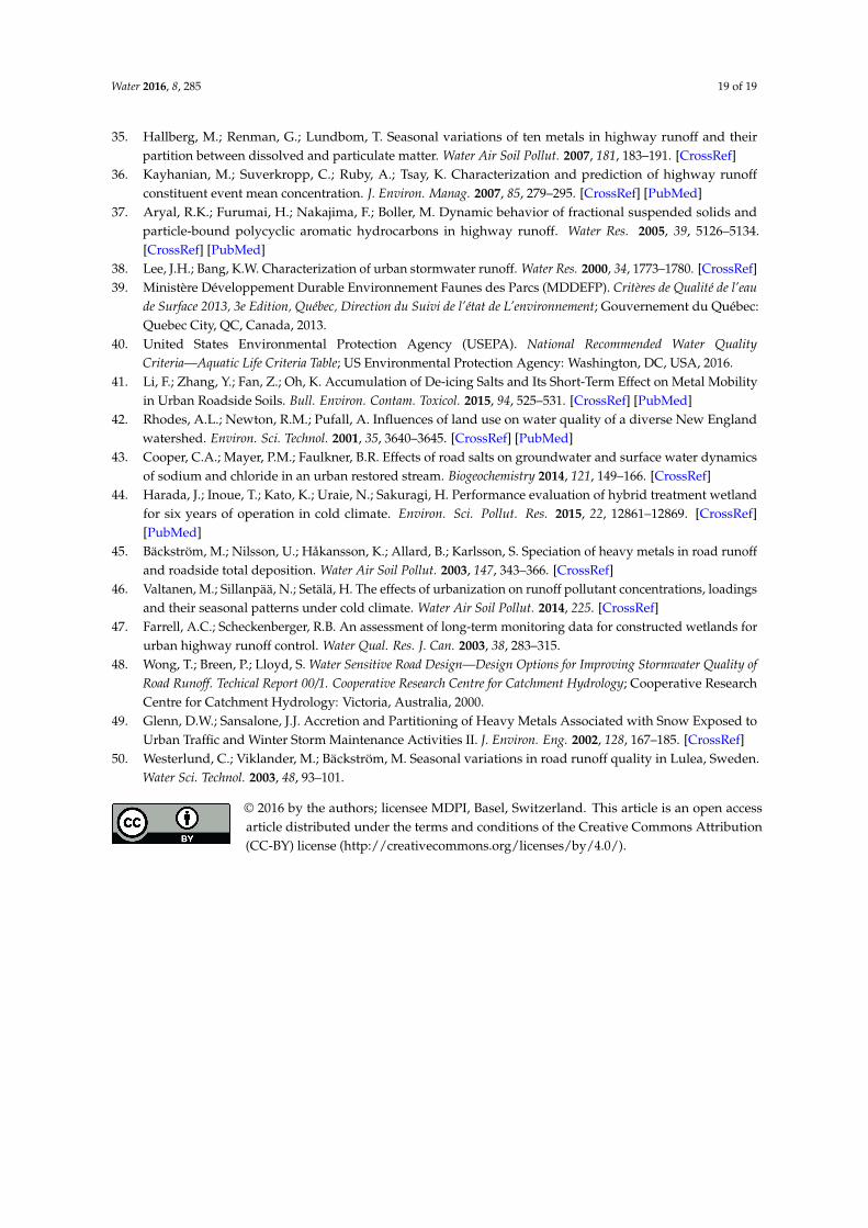
Water 2016, 8, 285 19 of 19
35. Hallberg, M.; Renman, G.; Lundbom, T. Seasonal variations of ten metals in highway runoff and theirpartition between dissolved and particulate matter. Water Air Soil Pollut. 2007, 181, 183–191. [CrossRef]
36. Kayhanian, M.; Suverkropp, C.; Ruby, A.; Tsay, K. Characterization and prediction of highway runoffconstituent event mean concentration. J. Environ. Manag. 2007, 85, 279–295. [CrossRef] [PubMed]
37. Aryal, R.K.; Furumai, H.; Nakajima, F.; Boller, M. Dynamic behavior of fractional suspended solids andparticle-bound polycyclic aromatic hydrocarbons in highway runoff. Water Res. 2005, 39, 5126–5134.[CrossRef] [PubMed]
38. Lee, J.H.; Bang, K.W. Characterization of urban stormwater runoff. Water Res. 2000, 34, 1773–1780. [CrossRef]39. Ministère Développement Durable Environnement Faunes des Parcs (MDDEFP). Critères de Qualité de l’eau
de Surface 2013, 3e Edition, Québec, Direction du Suivi de l’état de L’environnement; Gouvernement du Québec:Quebec City, QC, Canada, 2013.
40. United States Environmental Protection Agency (USEPA). National Recommended Water QualityCriteria—Aquatic Life Criteria Table; US Environmental Protection Agency: Washington, DC, USA, 2016.
41. Li, F.; Zhang, Y.; Fan, Z.; Oh, K. Accumulation of De-icing Salts and Its Short-Term Effect on Metal Mobilityin Urban Roadside Soils. Bull. Environ. Contam. Toxicol. 2015, 94, 525–531. [CrossRef] [PubMed]
42. Rhodes, A.L.; Newton, R.M.; Pufall, A. Influences of land use on water quality of a diverse New Englandwatershed. Environ. Sci. Technol. 2001, 35, 3640–3645. [CrossRef] [PubMed]
43. Cooper, C.A.; Mayer, P.M.; Faulkner, B.R. Effects of road salts on groundwater and surface water dynamicsof sodium and chloride in an urban restored stream. Biogeochemistry 2014, 121, 149–166. [CrossRef]
44. Harada, J.; Inoue, T.; Kato, K.; Uraie, N.; Sakuragi, H. Performance evaluation of hybrid treatment wetlandfor six years of operation in cold climate. Environ. Sci. Pollut. Res. 2015, 22, 12861–12869. [CrossRef][PubMed]
45. Bäckström, M.; Nilsson, U.; Håkansson, K.; Allard, B.; Karlsson, S. Speciation of heavy metals in road runoffand roadside total deposition. Water Air Soil Pollut. 2003, 147, 343–366. [CrossRef]
46. Valtanen, M.; Sillanpää, N.; Setälä, H. The effects of urbanization on runoff pollutant concentrations, loadingsand their seasonal patterns under cold climate. Water Air Soil Pollut. 2014, 225. [CrossRef]
47. Farrell, A.C.; Scheckenberger, R.B. An assessment of long-term monitoring data for constructed wetlands forurban highway runoff control. Water Qual. Res. J. Can. 2003, 38, 283–315.
48. Wong, T.; Breen, P.; Lloyd, S. Water Sensitive Road Design—Design Options for Improving Stormwater Quality ofRoad Runoff. Techical Report 00/1. Cooperative Research Centre for Catchment Hydrology; Cooperative ResearchCentre for Catchment Hydrology: Victoria, Australia, 2000.
49. Glenn, D.W.; Sansalone, J.J. Accretion and Partitioning of Heavy Metals Associated with Snow Exposed toUrban Traffic and Winter Storm Maintenance Activities II. J. Environ. Eng. 2002, 128, 167–185. [CrossRef]
50. Westerlund, C.; Viklander, M.; Bäckström, M. Seasonal variations in road runoff quality in Lulea, Sweden.Water Sci. Technol. 2003, 48, 93–101.
© 2016 by the authors; licensee MDPI, Basel, Switzerland. This article is an open accessarticle distributed under the terms and conditions of the Creative Commons Attribution(CC-BY) license (http://creativecommons.org/licenses/by/4.0/).