Impedance boundaryconditions for general transient

hemodynamics and other things

Will Cousins (MIT)

Rachael Brag and Pierre Gremaud (NCSU)

Vera Novak (BIDMC), Daniel Tartakovsky (UCSD)

July 14, 2014

Overview

Long term goal: non-invasive continuous measurement ofcerebral blood flow (CBF)

• “cheap" measurements: Transcranial Doppler to measureblood flow velocity (BFV)

• patient database and analysis thereof• computational hemodynamics

Challenges

In increasing order of “stochasticity"

• closures for hemodynamics models:how to model what isn’t in the computational domain (BCs)

• uncertainties in models, geometries and parameters• uncertainties in data:

lack of gold standard method, patient biases

We need error bars to our predictions

This talk

• impedance boundary conditions (outflow)• machine learning for CBF data (inflow)

Example: systemic arterial tree

Outflow BCs are fundamental

• inflow vessels: few and "easy" to measure⇐ DATA• outflow vessels: many and hard to measure⇐ MODEL• vasculature is reactive (autoregulation)

Arterial flow model: single vessel

approach• not interested in flow details but in vascular networks

"throughput"• one-d is often (but not always!) good enough

• computational justification (Grinberg et al., ABE, (2011))• derived BCs are general: can be adapted to multi-d

Arterial flow model: single vessel

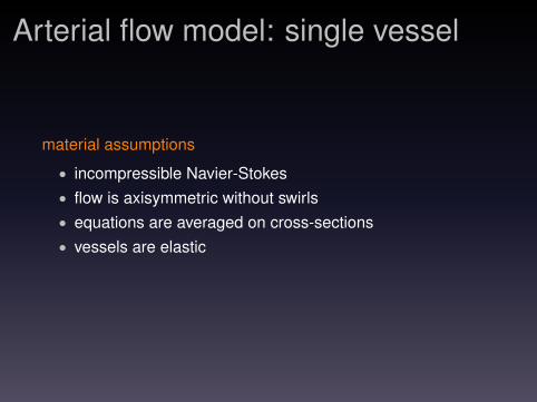
material assumptions

• incompressible Navier-Stokes• flow is axisymmetric without swirls• equations are averaged on cross-sections• vessels are elastic

Arterial flow model: single vessel

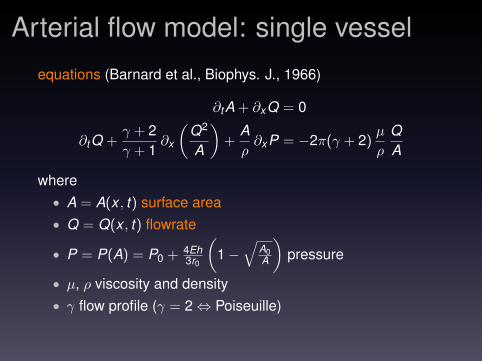
equations (Barnard et al., Biophys. J., 1966)

∂tA + ∂xQ = 0

∂tQ +γ + 2γ + 1

∂x

(Q2

A

)+

Aρ∂xP = −2π(γ + 2)

µ

ρ

QA

where• A = A(x , t) surface area• Q = Q(x , t) flowrate

• P = P(A) = P0 + 4Eh3r0

(1−

√A0A

)pressure

• µ, ρ viscosity and density• γ flow profile (γ = 2⇔ Poiseuille)

Arterial flow model: single vessel

Above equations are a system of hyperbolic balance lawsAt operating regime• solutions are smooth (no shock!)• Jacobian has one positive and one negative eigenvalue

We need

• one inflow condition (measured velocity)• one outflow condition

At junctions

• conservation of mass• continuity of pressure

Outflow BCs must

• mimic the part of the vasculature that is not modeled(downstream from computational domain)

• not create numerical artifacts• be cheap to run• be simple to implement• require a minimum of calibration

Outflow BCs: the classics

• Dirichlet (or Neumann) BC• impose a relationship between P and Q

• resistance:P = R Q

• RCR Windkessel:

P + R2 C ∂tP = (R1 + R2)Q + R1R2C ∂tQ

R. Saouti et al., Euro. Respir. Rev., 2010

Outflow BCs: the classics

• Dirichlet (or Neumann) BC• impose a relationship between P and Q

• resistance:P = R Q

• RCR Windkessel:

P + R2 C ∂tP = (R1 + R2)Q + R1R2C ∂tQ

Issues

• limited physiological basis• determination of parameter values

Impedance bc• takes the form of a convolution• zj ’s: impedance weights

Pn =n∑

j=0

zjQn−j + Pterm

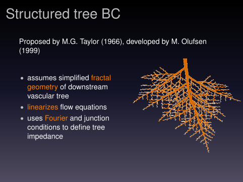
Structured tree BC

Proposed by M.G. Taylor (1966), developed by M. Olufsen(1999)

• assumes simplified fractalgeometry of downstreamvascular tree

• linearizes flow equations• uses Fourier and junction

conditions to define treeimpedance

New impedance BC

• Fourier→ Laplace:allows general flows (instead of just periodic ones)

• fractal structure→ effective tiered structure:greatly reduces need for calibration

• can be used in lieu of calibration for other BCs• better termination criterion

Tree geometry

Governed by four rules

rule 0: there are only bifurcationsrule 1: rd1 = α rp, rd2 = β rp

rule 2: ` = λ rrule 3: terminate vessel if r < rmin

where r is radius, ` is length and p and di are parent/daughters

Potential issue• scaling parameters are not constant (more later)

Linearization (in A about A0)

C ∂tP + ∂xQ = 0

∂tQ +A0

ρ∂xP = −2π(γ + 2)

µ

ρ

QA0

where C = dA/dP is the vessel compliance.

We Laplace transform and solve exactly

Q(0, s) = sdsCP(`, s) sinh(`

ds

)+ Q(`, s) cosh

(`

ds

)P(0, s) = P(`, s) cosh

(`

ds

)+

1sdsC

Q(`, s) sinh(`

ds

)

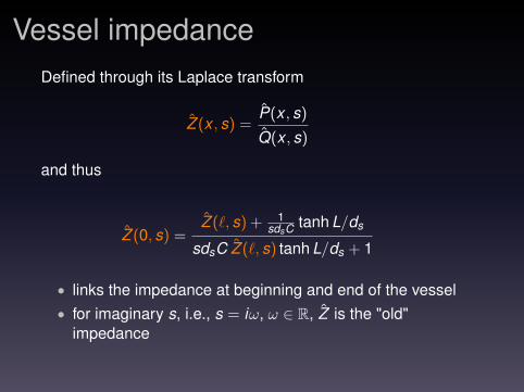
Vessel impedanceDefined through its Laplace transform

Z (x , s) =P(x , s)

Q(x , s)

and thus

Z (0, s) =Z (`, s) + 1

sdsC tanh L/ds

sdsC Z (`, s) tanh L/ds + 1

• links the impedance at beginning and end of the vessel• for imaginary s, i.e., s = iω, ω ∈ R, Z is the "old"

impedance

Tree impedance

can be defined recursively using junction conditions

• conservation of mass: Qp(`, t) = Qd1(0, t) + Qd2(0, t)• continuity of pressure: Pp(`, t) = Pd1(0, t) = Pd2(0, t)

⇒ 1Zpa(`, s)

=1

Zd1(0, s)+

1Zd2(0, s)

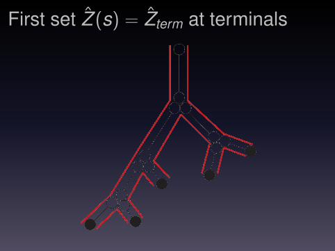
First set Z (s) = Zterm at terminals

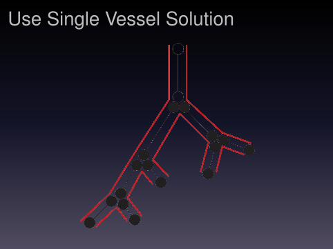
Use Single Vessel Solution

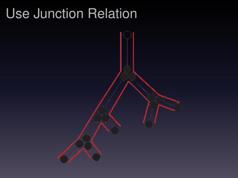
Use Junction Relation

Use Single Vessel Solution

Use Junction Relation

Use Single Vessel Solution

Use Single Vessel Solution

Use Junction Relation

Use Single Vessel Solution

Use Junction Relation

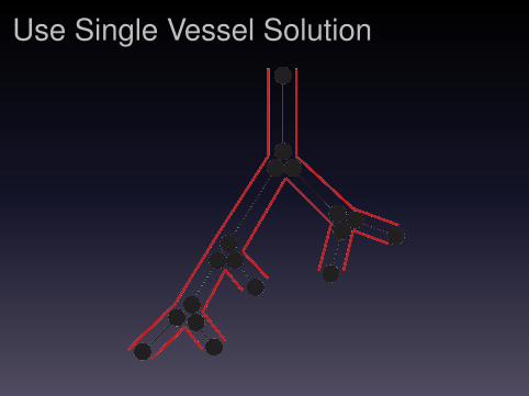
Use Single Vessel Solution

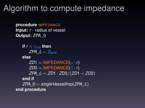
Algorithm to compute impedance

procedure IMPEDANCE

Input: r - radius of vesselOutput: ZPA_0

if r < rmin thenZPA_L = Zterm

elseZD1 = IMPEDANCE(α · r )ZD2 = IMPEDANCE(β · r )ZPA_L = ZD1 · ZD2/(ZD1 + ZD2)

end ifZPA_0 = singleVesselImp(ZPA_L)

end procedure

Implementation: intro

• we have just computed Z (s)

• convolution⇒ P(t) =∫ t

0 Z (τ) Q(t − τ) dτ

Problem: we need Z = L−1(Z ) and

L−1 is an ill-posed numerical nightmare

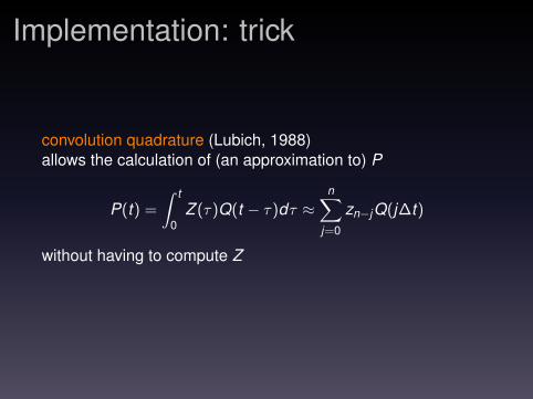
Implementation: trick

convolution quadrature (Lubich, 1988)allows the calculation of (an approximation to) P

P(t) =

∫ t

0Z (τ)Q(t − τ)dτ ≈

n∑j=0

zn−jQ(j∆t)

without having to compute Z

Implementation: CQ details

• Mellin’s inversion formula Z (τ) = 12πi

∫ ν+i∞ν−i∞ Z (λ)eλτ dλ

• Theorem If Zterm has nonnegative real part, then Z (s) isanalytic for all <s ≥ 0 except at s = 0, where it has aremovable singularity

• P(t) = 12πi

∫ ν+i∞ν−i∞ Z (λ) y(λ; t) dλ, y(λ; t) =

∫ t0 eλtQ(t − τ) dτ

• y as solution to ODE• discretize ODE through multistep method• re-express integral and efficient quadratures for Cauchy

integrals...

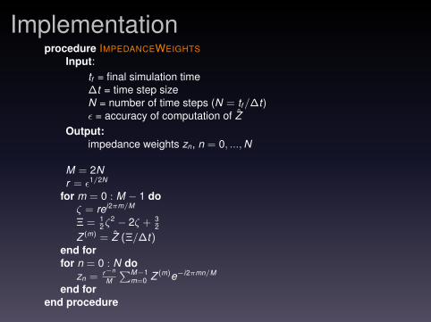
Implementationprocedure IMPEDANCEWEIGHTS

Input:tf = final simulation time∆t = time step sizeN = number of time steps (N = tf/∆t)ε = accuracy of computation of Z

Output:impedance weights zn, n = 0, ...,N

M = 2Nr = ε1/2N

for m = 0 : M − 1 doζ = rei2πm/M

Ξ = 12ζ

2 − 2ζ + 32

Z (m) = Z (Ξ/∆t)end forfor n = 0 : N do

zn = r−n

M

∑M−1m=0 Z (m)e−i2πmn/M

end forend procedure

Implementation: cost

• impedance weights computed for each outflow prior tosimulation

• requires 2N evaluations of Z• one eval. of Z = O((#generations)2) operations (a few

thousand)• in short: it is cheap

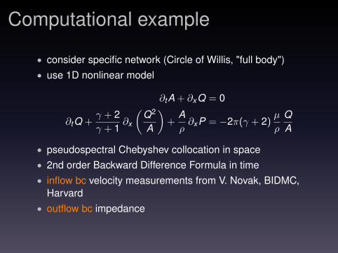
Computational example

• consider specific network (Circle of Willis, "full body")• use 1D nonlinear model

∂tA + ∂xQ = 0

∂tQ +γ + 2γ + 1

∂x

(Q2

A

)+

Aρ∂xP = −2π(γ + 2)

µ

ρ

QA

• pseudospectral Chebyshev collocation in space• 2nd order Backward Difference Formula in time• inflow bc velocity measurements from V. Novak, BIDMC,

Harvard• outflow bc impedance

Look Ma’ No calibration!

Some implementation details

• rmin taken as 30µm• Zterm = 0 is a terrible idea

Can be corrected through

Pn =n∑

j=0

zjQn−j + Pterm

with Pterm ≈ 45 mmHg

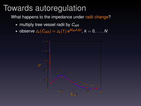
Towards autoregulationWhat happens to the impedance under radii change?

• multiply tree vessel radii by CAR

• observe zk (CAR) ≈ zk (1) eMARk∆t , k = 0, . . . ,N

Towards autoregulation (2)

• match has been checked over wide range of parameters• “memory" of structured tree ≈ .25 sec• time scale of autoregulation responses ≈ 5-20 sec• ⇒ auto-regulation induced microvascular changes

zk (MAR(t)) = zkeMAR(t)k∆t , k = 0, . . . ,N.

• scalar (!) MAR is obtained from specific autoregulationmodel

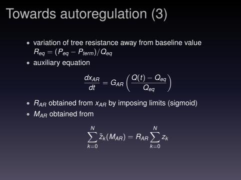
Towards autoregulation (3)

• variation of tree resistance away from baseline valueReq = (Peq − Pterm)/Qeq

• auxiliary equation

dxAR

dt= GAR

(Q(t)−Qeq

Qeq

)• RAR obtained from xAR by imposing limits (sigmoid)• MAR obtained from

N∑k=0

zk (MAR) = RAR

N∑k=0

zk

Towards autoregulation (4)• impose P(t) = Pbaseline(t)f (t) at aorta• 20% drop in MAP• immediate flow decrease followed by return to baseline

0 5 10

10

15

20

25

30

35

40

Time (s)

CB

V (cm

/ s

)

0 5 10

60

70

80

90

100

110

120

Time (s)

AP

(m

mH

g)

0 5 103

2.5

2

1.5

1

0.5

0

Time (s)

xA

R

0 5 10

0.8

0.85

0.9

0.95

1

Time (s)

RA

R

Database from BIDMC

total male femaleparticipants 167 86 81age 66.5±8 65.6±9 67.3±8.group hyper % no hyper % total %control 14 8.4 48 28.7 62 37.1stroke 26 15.6 16 9.6 42 25.1DM 36 21.6 27 16.2 63 37.7

Database from BIDMC (2)

For each patient: MCA data

BFV post-processed from Trans Cranial Doppler (TCD)CBF from CASL MRIHCT, CO2 from labage, height, weight from labhead size (front to back and side to side) from labgender, diabetes (y/n), hypertension (y/n) from labradius R from imagesinsonation angle θ from images

M territory mass from “maps" and post processing

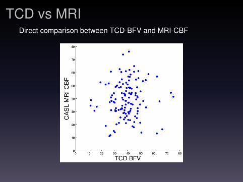
TCD vs MRIDirect comparison between TCD-BFV and MRI-CBF

TCD vs MRI (2)Direct estimate: CBFTCD = πR2

Mv

2 cos θ

Sources of uncertainties, TCD

• insonation angle• velocity profile• vessel radius• territory mass

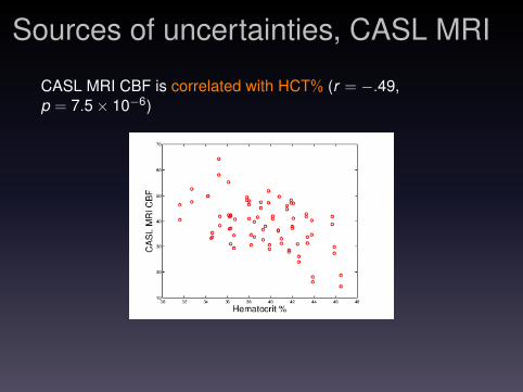
Sources of uncertainties, CASL MRI

CASL MRI CBF is correlated with HCT% (r = −.49,p = 7.5× 10−6)

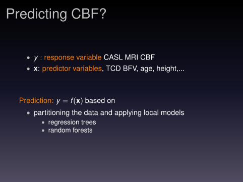
Predicting CBF?

• y : response variable CASL MRI CBF• x: predictor variables, TCD BFV, age, height,...

Prediction: y = f (x) based on

• partitioning the data and applying local models• regression trees• random forests

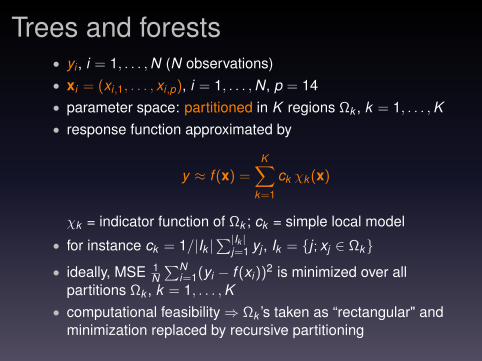
Trees and forests• yi , i = 1, . . . ,N (N observations)• xi = (xi,1, . . . , xi,p), i = 1, . . . ,N, p = 14• parameter space: partitioned in K regions Ωk , k = 1, . . . ,K• response function approximated by

y ≈ f (x) =K∑

k=1

ck χk (x)

χk = indicator function of Ωk ; ck = simple local model

• for instance ck = 1/|Ik |∑|Ik |

j=1 yj , Ik = j ; xj ∈ Ωk

• ideally, MSE 1N∑N

i=1(yi − f (xi))2 is minimized over allpartitions Ωk , k = 1, . . . ,K

• computational feasibility⇒ Ωk ’s taken as “rectangular" andminimization replaced by recursive partitioning

Trees and forests (2)Trees as above can be unstable. Improvements:

• consider an ensemble of trees (bootstrapping)• consider fixed number of predictive variables for splitting

⇒ decreases tree correlation and estimate variance

0

0.1

0.2

0.3

0.4

0.5

0.6

0.7

0.8

0.9

1 2 3 4 5 6 7 8 9 10 11 12 13Number of Randomly Selected Fitting Variables m

Cor

rela

tion

Betw

een

Tree

s

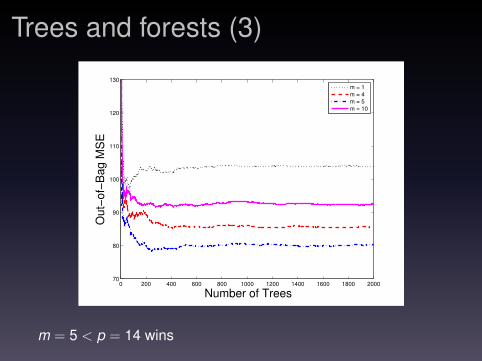
Trees and forests (3)

0 200 400 600 800 1000 1200 1400 1600 1800 200070

80

90

100

110

120

130

Number of Trees

Ou

t−of−

Ba

g M

SE

m = 1

m = 4

m = 5

m = 10

m = 5 < p = 14 wins

Some results: correlation

0 10 20 30 40 50 60 70 80 900

10

20

30

40

50

60

70

80

90

CBF out−of−bag prediction

CA

SL M

RI

Some results: variable importance

−0.2 −0.1 0 0.1 0.2 0.3 0.4 0.5 0.6

TCD BFVC02

WeightAge

Head WidthTerr. Mass

HCT %HeightAngle

GenderDiabetes

Head LengthArea

Hypertension

Average Error Increase

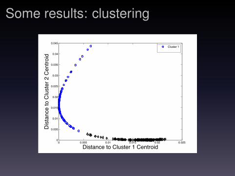
Some results: clustering

0 0.005 0.01 0.015 0.02 0.0250

0.005

0.01

0.015

0.02

0.025

0.03

0.035

0.04

0.045

Distance to Cluster 1 Centroid

Dis

tanc

e to

Clu

ster

2 C

entro

id

Cluster 1Cluster 2

Future work

• organ specific BCs• analysis of role played by calibration• efficient uncertainty representation in comp.

hemodynamics• local regression methods for patient clustering

references

• W. Cousins, P. Gremaud, Boundary conditions forhemodynamics: The structured tree revisited, J. Comput.Phys., 231 (2012), pp. 6068–6096.

• W. Cousins, P. Gremaud, D. Tartakovsky, A newphysiological boundary condition for hemodynamics, SIAMJ. Appl. Math., 73 (2013), pp. 1203–1223.

• W. Cousins, P. Gremaud, Impedance boundary conditionsfor general transient hemodynamics, Int. J. Numer. Meth.Biomed. Eng., in press.

• R. Bragg, P. Gremaud, V. Novak, Cerebral blood flowmeasurements: intersubject variability using MRI andTranscranial Doppler, in preparation