Embed Size (px)
Citation preview

Imperative-Program Transformation by
Instrumented-Interpreter Specialization†
Søren Debois ([email protected])IT University of Copenhagen‡; Programming, Logic, and Semantics Group
Abstract. We describe how to implement strength reduction, loop-invariant codemotion and loop quasi-invariant code motion by specializing instrumented inter-preters. To curb code duplication intrinsic to such specialization, we introduce anew program transformation, rewinding , which uses Moore-automata minimizationto remove duplicated code.
Keywords: Partial evaluation, interpretive approach, imperative program transfor-mation, code duplication, Moore automata.
CCS Codes: D.3.4, F.3.2.
1. Introduction
In this paper, we describe how to implement the imperative programtransformations strength reduction, loop-invariant code motion, andloop quasi-invariance hoisting (Song et al., 2000) by specializing instru-mented interpreters. Further, we introduce a novel program transforma-tion, rewinding, which uses Moore-automata minimization to removecode duplication.
This contribution is significant for at least the following reasons.First, we provide simple alternative implementations for well-known,non-trivial imperative program transformations. Second, implement-ing program transformation by instrumented interpreter specialization,also known as the interpretive approach (Gluck and Jørgensen, 1994), isnot well-studied for imperative languages. We provide insight into thestrengths and weaknesses of the interpretive approach in this setting.Finally, we provide both theoretical insight into the nature of codeduplication as well as rewinding as a practical remedy.
Our specializer is standard except for the rewinding transformation,which is straightforward to implement as a variant of Moore automataminimization. The relative simplicity of our interpreters thus suggeststhat constructing and specializing instrumented interpreters might bea feasible way to construct optimizing compilers for domain-specific
† This paper is a revised and extended version of the conference paper (Debois,2004).
‡ Rued Langgaardsvej 7, 2300 Copenhagen S, Denmark
c© 2006 Kluwer Academic Publishers. Printed in the Netherlands.
hosc06.tex; 7/03/2006; 12:47; p.1

2
languages. In this way our results complement recent findings (Thibaultet al., 2000) that compiling domain-specific languages by specializationcan yield target programs performing comparably to hand-coded low-level programs.
How does the interpretive approach apply in an imperative setting?We instrument an interpreter to collect statically available informationas it runs, thus establishing an execution history, which is subsequentlyused to justify transformations. For example, an interpreter may per-form loop-invariant code motion on an assignment x := <exp> bychecking whether a particular execution of the assignment could changethe value of x. If it would not, the interpreter simply skips the as-signment. The interpreter uses the execution history to approximatewhether executing the assignment would change x.
If a program point is reachable in more than one way, there may bemore than one possible history for it. Thus, polyvariant specializationof history-collecting interpreters sometimes introduces code duplica-tion, much the same way that polyvariant specialization of programswith dead static variable does (Gomard and Jones, 1991; Jones et al.,1993; Jones, 2004). This duplication is intrinsic to our methods; wecannot prevent it. Instead, we apply our rewinding transformation tothe residual program, thereby removing duplication. Rewinding of aprogram proceeds by translating the program into a Moore automa-ton, minimizing that Moore automaton, and translating the minimizedautomaton back into a program. We shall see (Corollary 15, page 23)that rewinding preserves semantics.
We believe that ours is the first substantial application of the inter-pretive approach to an imperative language (although (Thibault et al.,2000) contain an application to a domain-specific imperative language).For functional languages, the interpretive approach has been used todo constant propagation and higher-order removal (Sperber and Thie-mann, 1996), super-compilation (Gluck and Jørgensen, 1994; Gluck andJørgensen, 1994) and deforestation (Gluck and Jørgensen, 1994).
We expect the reader to have a basic proficiency in partial eval-uation, corresponding to the level of (Jones et al., 1993). A passingfamiliarity with the interpretive approach (Gluck and Jørgensen, 1994)and automata theory (Hopcroft and Ullman, 1979) would be helpful,but is not required.
This paper is organized as follows. In Section 2, we introduce theFlowchart language, a Flowchart interpreter, and a Flowchart special-izer; in Section 3, we describe how to implement loop-invariant codemotion and loop quasi-invariant hoisting; in Section 4, we describe howto implement strength reduction; in Section 5, we investigate codeduplication; in Section 6, we define rewinding and prove it semantic
hosc06.tex; 7/03/2006; 12:47; p.2

3
preserving; and in Section 7, we discuss our methods and give directionsfor future work.
2. Preliminaries
We use a variant of the Flowchart language of (Gomard and Jones,1991; Jones et al., 1993). Syntax for the language is given in Figure1; Id is the set of identifiers (variable names). A program is a list ofinput variables and a sequence of basic blocks, each of which is a seriesof assignments followed by a jump (goto), a conditional jump (if) orprogram termination (return). Notice that the flowchart language doesnot encompass pointer variables.
Program ::= Input Block+
Input ::= read Id∗
Block ::= Label Asgns Jump
Jump ::= goto Label
| if Param then Label else Label
| return Param
Asgns ::= Asgn∗
Asgn ::= Id := Expr
Expr ::= Op Param+
| Param
Param ::= Id
| ‘ SExp
SExp ::= atom
| ( SExp∗ )
Op ::= hd | tl | cons | + | - | = | < | . . .
Figure 1. The Flowchart Language
We assume throughout that there are no jumps to undefined labels,that the label of each basic block is unique, and that each operatorapplication has the correct number of parameters. We allow as syn-tactic sugar if, while, and case; compound expressions; infix cons
operator ::; short-circuiting boolean expressions; macros; labels insidebasic blocks; and anonymous entry blocks. See Figure 4 for a simpleexample program.
Values for the Flowchart language are the S-expressions of LISP;that is, values are either atoms or pairs of values, atoms being eitherstrings or numbers. The semantics of the Flowchart is as expected withexecution commencing at the first basic block, the entry block.
hosc06.tex; 7/03/2006; 12:47; p.3

4
Definition 1. (Semantics of Flowchart) Let P be a Flowchart pro-gram, and let l be a label of P . We write blc to mean the basic block of P
with label l. Let V be some non-empty set of values with False ∈ V .An environment is a finite map σ : Id → V ; we write IE for the set of allenvironments. We assume total functions J·KA : Asgns → IE → IE, forexecuting assignments; and J·KP : Param→ IE → V , for evaluating pa-rameters. (The simple interpreter of Figure 3 implements J·KA and J·KP
in the natural way.) Define a function J·KJ : Jump → IE → Label × IE
by
Jgoto lKJ σ = (l, σ)
Jif p then l1 else l2KJ σ =
{
(l2, σ) if JpKP σ = False
(l1, σ) otherwise
Jreturn pKJ σ = (•, σ[Y ← JpKP σ]),
where • is different from all labels and Y is different from all vari-able names. Define a total function J·KB : Block → IE → Label × IE
by Jl Asgns JumpKB σ = JJumpKJ (JAsgnsKA σ). A run of length n of P
on environment σ1 is a sequence (l1, σ1) . . . (ln, σn) such that li 6= •for 1 ≤ i < n, (li, σi) = Jbli−1cKB σi−1 for 1 < i ≤ n, and l1 is the labelof the entry block of P . We say that P terminates on σ1 with value v
if there exists a run (l1, σ1) . . . (ln, σn) such that ln = • and σn(Y ) = v.We define a semantic function JP K : IE → V⊥ by
JP Kσ =
{
v if P terminates on σ with value v
⊥ otherwise.
Two programs P and P ′ are semantically equivalent iff JP K = JP ′K.
We implement Flowchart interpreters in Flowchart itself extendedwith an indexed store construct, which is handy for implementingenvironments in Flowchart self-interpreters. The extended language,Flowchart+, has the two extra constructs shown in Figure 2: A new
...Asgn ::= . . .
| [ Param ] := Param...
Op ::= . . . | load
Figure 2. The Flowchart+ Language
assignment form allows the assignment of a value to a store location,
hosc06.tex; 7/03/2006; 12:47; p.4
5
and a new operator allows the retrieval of a value from a store location.We use ‘[Param]’ as syntactic sugar for ‘load Param’.
A Flowchart-interpreter written in Flowchart+ is given in Figure 3.Programs are represented in the obvious manner: a program is a list ofblocks, a block is a 3-tuple, and so forth. Execution commences at line 9;the first 8 lines include convenient macros (relegated to Appendix A)and define a macro for evaluating parameters. The interpreter movesthe actual parameters into the store (lines 11–15) and proceeds to thebasic-block executing loop (lines 18–63). The basic block to be executedis fetched and split into constituent parts (lines 19–20), whereafter theassignments of the current block are executed (lines 21–47) by evaluat-ing the parameters (lines 26–32), and applying the appropriate operatorto the values of the parameters (lines 33–45). Finally, the jump of thebasic block is executed (lines 48–63). (The label next-asgn is not usedbefore we instrument the interpreter in the next section.)
The Specializer To do our experiments, we have implemented a rudi-mentary polyvariant, transition-compressing, program-point specializerfrom Flowchart+ to Flowchart, as described in (Jones et al., 1993).We restrict our attention to Flowchart+-programs in which every storeaccess is to a statically known location; this restriction ensures thatstore locations can be replaced by variable accesses in the residual pro-gram. Naturally, all of our interpreters are in this class of Flowchart +
programs.Our specializer applies the rewinding transformation after speciali-
zation proper, to remove code duplication in residual programs. (Wediscuss rewinding in detail in Sections 5 and 6.) All the residual pro-grams exhibited in this paper are actual output of our specializer.
A note on terminology To avoid the awkward phrase “P is the re-sult of specializing interpreter int w.r.t. program P ′” we shall say“P ′ transformed by int yields P”. This slight abuse of language em-phasizes the intuition that an instrumented interpreter implements atransformation.
3. Loop-Invariant Code Motion
Loop-invariant code motion (Muchnick, 1997) identifies computationsin loops that yield the same value on every iteration and moves suchcomputations out of the loop. Consider the program in Figure 4. Givena positive natural number n, this program computes (2n − 1)!. Theassignment t := 2 * n in line 5 is recomputed on each iteration of
hosc06.tex; 7/03/2006; 12:47; p.5

6
1 include "macros.i"macro eval-param (p) :
case hd p of4 ‘quote: return tl p;
‘id: return [tl p];default: return ‘(malformed param);end;
8 endread pgm, data;
formals := tl (hd pgm);while formals != ‘() do
12 [hd formals] := hd data;formals := tl formals;data := tl data;
end;16 bbs := hd (tl pgm);
next := hd (hd bbs);exec-bb:
bb := lookup (next, bbs);20 asgns := hd bb; jump := tl bb;
while asgns != ‘() doasgn := hd asgns; asgns := tl asgns;id := hd asgn; exp := tl asgn;
24 op := hd exp; params := tl exp;param1 := ‘(); param2 := ‘();if params != ‘() do
param1 := eval-param (hd params);28 params := tl params;
end;if params != ‘() do
param2 := eval-param (hd params);32 end;
case op of‘hd: [id] := hd param1;‘tl: [id] := tl param1;
36 ‘not: [id] := ! param1;‘base: [id] := param1;‘eq: [id] := param1 = param2;‘cons: [id] := cons (param1,param2);
40 ‘add: [id] := param1 + param2;‘mult: [id] := param1 * param2;‘less: [id] := param1 < param2;default:
44 return ‘(bad operator);end;
next-asgn:end;
48 case hd jump of‘goto:
next := tl jump;‘return:
52 return eval-param (tl jump);‘if:
param := hd (tl jump);labtrue := hd (tl (tl jump));
56 labfalse := tl (tl (tl jump));if eval-param (param) do
next := labtrue;else
60 next := labfalse;end;
end;goto exec-bb;
Figure 3. A simple interpreter for Flowchart.
hosc06.tex; 7/03/2006; 12:47; p.6

7
1 read n;f := 1;i := 1;
4 loop:t := 2 * n;again := i < t;if again then body else done;
8 body:f := f * i;i := i + 1;goto loop;
12 done:return f;
Figure 4. Program fac.
the loop, even though the value of n never changes. We shall see howtransforming fac by an instrumented interpreter may yield the programin Figure 7.
Executing an assignment x := <exp> cannot change the value of xif (a) the previous assignment to x were also x := <exp> and (b) thevariables used in <exp> were not updated in the meantime. If theseconditions are satisfied, we say that the assignment x := <exp> isavailable.
Maintaining a list of available assignments is easy in an interpreter.Every time an assignment x := <exp> has been executed, we removeall assignments that use or define x from the available assignments list.Then we add the assignment x := <exp> to the list, provided <exp>
does not reference x. The available assignments are a subset of theassignments of the input program, so the available assignments listis of bounded static variation (Jones et al., 1993). Thus, recordingavailable assignments does not introduce extra specialization-time non-termination in the interpreter.
A code fragment maintaining the available assignments list is givenin Figure 5. The fragment is inserted immediately after the code for
1 tmp := ‘();while available != ‘() do
asgn’ := hd available;4 if !(member (id, use (asgn’)) || def (asgn’) = id) do
tmp := cons (asgn’, tmp);end;available := tl available;
8 end;available := reverse (tmp);if !(member (id, use (asgn))) do
available := cons (asgn, available);12 end;
Figure 5. Implementation of available assignments analysis.
execution of an assignment — that is, between line 45 and line 46in Figure 3. Suppose an assignment id := <exp> has just been exe-
hosc06.tex; 7/03/2006; 12:47; p.7

8
cuted. First, any previously available assignments that use or define idare removed from the list (lines 1–9). Then the current assignment isadded to the list of available assignments, provided it is not a self-assignment (lines 10–12). The macros reverse, member, use and def
compute list reversal, list membership, the list of variables referenced inan assignment and the variable defined by an assignment, respectively.
The code fragment in Figure 6 skips execution of superfluous assign-ments. It is inserted immediately before the code for assignment execu-tion — that is, between line 24 and line 25 of Figure 3. The fragmentsearches the list of available assignments for the current assignment,which is skipped if found.
1 tmp := available;while tmp != ‘() do
asgn’ := hd tmp;4 if asgn = asgn’ do goto next-asgn; end;
tmp := tl tmp;end;
Figure 6. Implementation of superfluous assignment skipping.
Augmenting the simple interpreter of Figure 3 with these fragments,we obtain the hoisting interpreter. Transforming the fac program ofFigure 4 by the hoisting interpreter yields the program in Figure 7.The non-contiguous label names L0, L3 and L4 are an artifact of our
1 read data;L0:
n := hd data;4 f := 1;
i := 1;t := 2 * n;again := i < t;
8 if again then L3 else L4;L3:
f := f * i;i := i + 1;
12 again := i < t;if again then L3 else L4;
L4:return f;
Figure 7. Transformation of fac (Figure 4) by the hoisting interpreter.
specializer applying rewinding to remove code duplication; refer toSection 5 for details.
The test part of the loop (lines 5–7 of the original program in Fig-ure 4) has been unrolled once in the residual program in Figure 7: inthe first iteration (lines 6–8), t := 2 * n is computed; in subsequentiterations (lines 12–13), it is skipped. This unrolling occurs becausethe value of the variable available is static: Each basic block of theinput program occurs in the output program once for each possible
hosc06.tex; 7/03/2006; 12:47; p.8

9
value of available. For the fac program, the value of available atthe first iteration of loop is
[i := 1, f := 1],
whereas on the second iteration onwards it is
[t := 2 * n].
(The statement again := i < t is not available because of subsequentassignment to i; similarly, the statements f := f * i and i := i +
1 are not available because they are self-assignments.) Thus, the loop
block occurs twice in the output: in lines 5–8 and lines 12–13.However, the assignment t := 2 * n appears only in the first oc-
curence, not in the second. On the second iteration of loop, the in-terpreter skips the execution of t := 2 * n precisely because it is inavailable (see Figure 6); hence, that statement does not occur in theoutput program.
The transformation achieved by the hoisting interpreter is slightlydifferent from what is usually understood by loop-invariant code mo-tion: Rather than moving the invariant assignment t := 2 * n outsideof the loop, we have instead unrolled the loop, in the process removingthe redundant computation from the second iteration onwards. Un-rolling the loop reduces loop-invariant code motion to a trivial case ofcommon-subexpression elimination.
This implementation also does loop quasi-invariant hoisting (Songet al., 2000). This is a loop optimization in which one recognizes thatafter some finite number of iterations, an assignment in the loop be-comes invariant. Figure 8 contains an example. The basic blocks loop
1 read n;i := 0;sum := 0;
4 x1 := 0;x2 := 0;
loop:t := i < n;
8 if t then body else done;body:
x3 := x2 + 1;x2 := x1 + 1;
12 x1 := 2 * n;sum := sum + x3;i := i + 1;goto loop;
16 done:return sum;
Figure 8. Opportunity for loop quasi-invariance code motion.
and body forms a loop, in which x1 is constant from the second itera-tion, x2 is constant from the third iteration, and x3 is constant from the
hosc06.tex; 7/03/2006; 12:47; p.9

10
iteration available
1 [x2 := 0, x1 := 0, sum := 0, i := 0]
2 [x1 := 2 * n]
3 [x2 := x1 + 1, x1 := 2 * n]
4 [x3 := x2 + 1, x2 := x1 + 1, x1 := 2 * n]
Figure 9. The value of available at the block loop.
fourth iteration. We would expect a clever optimizing compiler to unrollthe loop precisely four times, successively removing the loop-invariantcomputations of x1, x2 and x3.
Our implementation does loop quasi-invariance hoisting. On the sec-ond iteration of the loop, the hoisting interpreter skips x1 := 2 * n
because it is available. Thus x1 is not modified, so x2 := x1 + 1 isavailable on the third iteration. Similarly, x3 is avilable on the fourthiteration, on which available stabilizes. (The values of available forloop are listed in Figure 3.) Thus, the block loop occurs four times inthe output: once for each value of available.
Transforming the program of Figure 8 by the hoisting interpreteryields the program in Figure 10. The loop has been unrolled four timeswith the assignments to x1, x2 and x3 successively eliminated.
Although the program of Figure 8 is admittedly contrived, it is sug-gested in (Song et al., 2000) that opportunities for loop quasi-invarianthoisting are not uncommon in automatically generated programs.
4. Strength Reduction
Consider the program div of Figure 11. This program computes thefunction
f(n, e) = 3
⌈
n
3e
⌉
, n, e ∈ IN,
where dxe is the least integer greater than or equal to x. The vari-able j will assume the values 0, 3e, 6e, 9e, . . ., so we may replace line 9with j := j + (3 * e). The expression 3 * e is loop-invariant, so ifwe compute it outside of the loop and store the result in some freshvariable, say, v0 := 3 * e, we can change line 9 to j := j + v0. Ifaddition is faster than multiplication, this transformation may be anoptimization. Automatically converting multiplications to additions iscalled strength reduction (Muchnick, 1997).
In the above example, we replace i * e with j + (3 * e). Towardsinstrumenting an interpreter to do strength reduction, we consider the
hosc06.tex; 7/03/2006; 12:47; p.10

11
1 read data;L0:
n := hd data;4 i := 0;
sum := 0;x1 := 0;x2 := 0;
8 t := i < n;if t then L1 else L4;
L1:x3 := x2 + 1;
12 x2 := x1 + 1;x1 := 2 * n;sum := sum + x3;i := i + 1;
16 t := i < n;if t then L3 else L4;
L3:x3 := x2 + 1;
20 x2 := x1 + 1;sum := sum + x3;i := i + 1;t := i < n;
24 if t then L5 else L4;L4:
return sum;L5:
28 x3 := x2 + 1;sum := sum + x3;i := i + 1;t := i < n;
32 if t then L7 else L4;L7:
sum := sum + x3;i := i + 1;
36 t := i < n;if t then L7 else L4;
Figure 10. Transformation of the program of Figure 8 by the hoisting interpreter.
1 read n, e;i := 0;j := 0;
4 loop:t := j < n;if t then body else done;
body:8 i := i + 3;
j := i * e;goto loop;
done:12 return i;
Figure 11. Program div.
relationship of these variables when we are about to evaluate i * e.Using i, e and j to denote the values of i, e and j, respectively, andusing i′ to denote the previous value of i, we find
j = i′e
i = i′ + 3(1)
Thusie = (i′ + 3)e = i′e + 3e = j + 3e. (2)
hosc06.tex; 7/03/2006; 12:47; p.11

12
Because i * e evaluates to ie, we may substitute j + (3 * e) for it,provided the values of i, j and e are related by some value i′ as specifiedin (1). Obviously, we can generalize the “3” to an arbitrary constant c.In this case
j = i′e
i = i′ + c(3)
andie = (i′ + c)e = i′e + ce = j + ce.
Thus, for any constant c, we may replace i * e with j + (c * e),provided the values i, e and j are related by some i′ as specified by (3)This condition is quite general; for example, it says neither that i and j
should occur within a loop, nor that the value i′ should be the previousvalue of i.
We restrict our attention to a simple case sufficient to do strengthreduction on the div program. Consider a sequence of assignments
j := i * e, . . . , i := i + c, . . . , j := i * e. (4)
Any such sequence produces values satisfying (3), provided that e isconstant throughout it and that it contains no other definitions of iand j. By recording a history of recent assignments, an interpretercan check whether the assignments executed so far constitute such asequence; we call this history the reaching definitions. The reaching def-initions differ from the available assignments of the hoisting interpreterin that they may contain assignments that are no longer available.
The interpreter variable that stores the reaching definitions must beof bounded static variation. We ensure this boundedness by recording atmost one assignment for each variable of the input program, replacingolder assignments with newer ones as we go.
The actual strength reduction is performed by the interpreter re-placing the statement j := i * e with the statements v0 := c * e
and j := j + v0, where v0 is some fresh variable name. Loop-invarianthoisting can then move the former statement out of the loop.
When j := i * e has been strength reduced to j := j + e, wemust be careful to put the original assignment j := i * e in thereaching definitions. If we insert the strength-reduced alternative as-signments, then on the next iteration of the loop, the interpreter willfind the reaching definitions sequence
j := j + e, . . . , i := i + c, . . . , j := i * e.
This sequence does not have the form (4), so there will be no strengthreduction. In the implementations below, the revision variable recordsthe necessity of revising the reaching definitions.
hosc06.tex; 7/03/2006; 12:47; p.12

13
Strength reduction is implemented in Figure 12 (collecting reachingdefinitions) and 13 (recognizing sequences of the form (4) and actuallyperforming strength reduction). The former is to be inserted along withthe available assignments computation (Figure 5) between line 45 andline 46 of the simple interpreter (Figure 3), the latter is to be insertedalong with the hoisting implementation (Figure 6) between line 25 andline 26.
1 if revision != ‘() doasgn’ := hd revision;revision := tl revision;
4 elseasgn’ := asgn;
end;left := reaching;
8 right := ‘();while left != ‘() do
asgn’’ := hd left;if def (asgn’’) = def (asgn’) then
12 cutoff;right := cons (asgn’’, right);left := tl left;
end;16 cutoff:
reaching := asgn’ :: reverse (right);
Figure 12. Implementation of reaching definitions analysis.
The implementation of strength reduction in Figure 13 derives itscomplexity mostly from the unsuitability of Flowchart for list process-ing. The implementation simply scans the reaching definitions, startingat the most recent one, checking if they are on the form (4).
Note the construction of a name for the necessary temporary variablein line 36. Exploiting that variable names, as represented in the inter-preter, are not restricted to atoms (i.e., the value of a cons-expressionis a legal variable name), the interpreter produces a name for thetemporary by concatenating the label of the current basic block withthe assignments remaining in the current basic block. Together, thesetwo uniquely identify an assignment in the input program. (Whenoutputting the residual program, our partial evaluator converts non-atomic variable names to strings of the form vn not otherwise presentin the residual program.)
Altogether, we have constructed the strength-reducing interpreter.Transforming the div program by the strength-reducing interpreteryields the program of Figure 14. Note the unrolling of the main loop:the first iteration establishes the preconditions, the second iterationcomputes the loop-invariant multiplication, and subsequent iterationsare strength reduced.
hosc06.tex; 7/03/2006; 12:47; p.13

14
1 if hd exp = ‘mult &&hd (param1Of (asgn)) = ‘id &&hd (param2Of(asgn)) = ‘id
4 doj := def (asgn);i := tl (param1Of (asgn));e := tl (param2Of (asgn));
8 rs := reaching;while rs != ‘() doasgn’ := hd rs; rs := tl rs;if i = def (asgn’) do
12 if ‘add = hd (tl asgn’) &&(‘id :: i) = param1Of (asgn’) &&‘quote = hd (param2Of (asgn’))
do16 c := tl (param2Of (asgn’));
goto found-incr;elsegoto abort-strength-reduction;
20 end;end;if j = def (asgn’) || e = def (asgn’) thenabort-strength-reduction;
24 end;goto abort-strength-reduction;
found-incr:while rs != ‘() do
28 asgn’ := hd rs; rs := tl rs;if asgn = asgn’then do-strength-reduction;
if i = def (asgn’) || e = def (asgn’)32 then abort-strength-reduction;
end;goto abort-strength-reduction;
do-strength-reduction:36 tmp := next :: asgns;
mult := mkBinOpAsgn (tmp, ‘mult,‘quote :: c,‘id :: e);
40 asgn’ := mkBinOpAsgn (j, ‘add,‘id :: j,‘id :: tmp);
asgns := mult :: asgn’ :: asgns;44 revision := mult :: asgn :: ‘();
goto next-asgn;abort-strength-reduction:
end;
Figure 13. Implementation of strength reduction.
5. Code Duplication
Consider the program count of Figure 15. Given an integer n and aninteger list xs, this program counts the number of elements of xs greaterthan n.
If we transform the count program by the hoisting interpreter, butomit post-specialization rewinding, we get the program in Figures 16and 17; the latter figure represents the program graphically, solid edgescorresponding to then-branches and dashed edges to else-branches.
hosc06.tex; 7/03/2006; 12:47; p.14

15
1 read data;L0:
n := hd data;4 data := tl data;
e := hd data;i := 0;j := 0;
8 t := j < n;if t then L1 else L2;
L1:i := i + 3;
12 j := i * e;t := j < n;if t then L3 else L2;
L2:16 return i;
L3:i := i + 3;v0 := 3 * e;
20 j := j + v0;t := j < n;if t then L9 else L2;
L9:24 i := i + 3;
j := j + v0;t := j < n;if t then L9 else L2;
Figure 14. Transformation of div (Figure 11) by the strength-reducing interpreter.
1 read n, xs;start:
i := 0;4 goto loop;
loop:t := xs = ‘();if t then done else body;
8 body:x := hd xs;xs := tl xs;t := n < x;
12 if t then inc else loop;inc:
i := i + 1;goto loop;
16 done:return i;
Figure 15. Program count.
The transformed program clearly contains redundant blocks. Com-paring it to the original, we see that the block L0 corresponds tothe concatenation of the start and loop blocks, modulo labels andargument-reading artifacts of the interpreter. This concatenation is aresult of transition compression. Moving on, L1 corresponds to done, L2to body, L3 to the concatenation of inc and loop (again concatenatedby transition compression) and L4 to loop. Altogether, the blocks L0
through L4 correspond to the entire input program, so we would preferthat there were no more blocks in the transformed program. Alas, thereare.
hosc06.tex; 7/03/2006; 12:47; p.15

16
1 read data;L0:
n := hd data;4 data := tl data;
xs := hd data;i := 0;t := xs = ‘();
8 if t then L1 else L2;L1:
return i;L2:
12 x := hd xs;xs := tl xs;t := n < x;if t then L3 else L4;
16 L3:i := i + 1;t := xs = ‘();if t then L5 else L6;
20 L4:t := xs = ‘();if t then L1 else L2;
L5:24 return i;
L6:x := hd xs;xs := tl xs;
28 t := n < x;if t then L7 else L8;
L7:i := i + 1;
32 t := xs = ‘();if t then L5 else L6;
L8:t := xs = ‘();
36 if t then L5 else L6;
Figure 16. Transformation of count (Figure 15) by the hoisting interpreter, omittingpost-specialization rewinding.
The blocks L3 and L4 both end with code corresponding to loop,so we would expect L3 and L4 to branch to the same continuations.However, they do not. Whereas the L4 block returns to either L1 or L2,the L3 block branches to either L5 and L6.
Both L1 and L5 correspond to done, and both L2 and L6 correspondto body. Similarly, both L7 and L3 correspond to the concatenationof inc and loop, and both L8 and L4 correspond to loop block.
Altogether, the transformation of count by the hoisting interpreterhas caused the main loop formed by loop, body and inc to be dupli-cated into the blocks L1 through L4 and the blocks L5 through L8.
Why is this? The available assignments at the loop block dependon the path taken to reach loop. If we arrive via start, then theassignment i := 0 is available. If we arrive via inc, then no assignmentto i is available, because of the self-assignment i := i + 1 in inc.Finally, if we arrive via body, then the available assignments for i
depends on the path taken to reach the body block, because the body
block does not itself change the availability of i.
hosc06.tex; 7/03/2006; 12:47; p.16

17
(L0)
n := hd data;data := tl data;xs := hd data;i := 0;t := xs = ‘();if t then L1 else L2;
(L1) return i;
(L2)
x := hd xs;xs := tl xs;t := n < x;if t then L3 else L4;
(L3)i := i + 1;t := xs = ‘();if t then L5 else L6;
(L4) t := xs = ‘();if t then L1 else L2;
(L6)
x := hd xs;xs := tl xs;t := n < x;if t then L7 else L8;
(L7)i := i + 1;t := xs = ‘();if t then L5 else L6;
(L8) t := xs = ‘();if t then L5 else L6;
(L5) return i;
Figure 17. Flowgraph representation of the program of Figure 16.
hosc06.tex; 7/03/2006; 12:47; p.17

18
Although the difference in available assignments does not affectthe hoisting interpreter’s subsequent actions, specialization is still per-formed once for each possible history — hence, code duplication. In theblocks L1 through L4, the assignment i := 0 is available, whereas inL5 through L8, no assignment for i is available.
The histories for i follow a pattern common to most loops: a variableis initialized to some value (one history), and subsequently updatedfor each iteration of a loop (a second history). The resulting codeduplication is compounded by consecutive loops, possibly leading toa residual program exponentially larger than the original program.
This duplication has the flavor of the dead static variable prob-lem (Gomard and Jones, 1991; Jones, 2004; Jones et al., 1993). Whereasthe dead static variable problem is easily solved by reclassifying deadstatic variables as dynamic, there is no simple way to avoid recordinguseless available assignments without defeating the purpose of easilyimplementing transformations. Thus, we settle for removing redun-dancy after specialization.
Looking at the duplicated blocks L1 and L5, we see that they areequivalent in the sense that they execute the same assignments, per-form the same test, and branch to similarly equivalent blocks. Thisnotion of equivalence resembles equivalence of states in Moore au-tomata (i.e., deterministic finite automata with labelled states). Inturn, this resemblance hints at a method for removing code duplica-tion in a program P : translate P to a Moore automaton, minimizethat automaton, and translate the minimized automaton back to aprogram P ′. We call this procedure rewinding. Without rewinding, theoutput programs exhibited in Sections 3 and 4 would contain variousdegrees of duplication.
In the next section, we define these translations; prove that theycommute with semantic equivalence and automata equivalence, respec-tively; and define rewinding formally. But first, let us see rewinding inaction: Applying the rewinding transformation to the residual programin Figure 16 and 17 yields the program in Figure 18. Note how theblocks L1 – L4 have been removed.
6. Rewinding & Moore Automata
In this section we translate programs to Moore automata and viceversa. The encodings are mutually inverse and ensure that equivalenceof Moore automata entail semantic equivalence of their correspondingprograms.
hosc06.tex; 7/03/2006; 12:47; p.18

19
1 read data;L0:
n := hd data;4 data := tl data;
xs := hd data;i := 0;t := xs = ‘();
8 if t then L5 else L6;L5:
return i;L6:
12 x := hd xs;xs := tl xs;t := n < x;if t then L7 else L8;
16 L7:i := i + 1;t := xs = ‘();if t then L5 else L6;
20 L8:t := xs = ‘();if t then L5 else L6;
Figure 18. Transformation of count (Figure 15) by the hoisting interpreter,including post-specialization rewinding.
We begin by recalling the definition of a Moore automaton (Hopcroftand Ullman, 1979). Intuitively, a Moore automaton is a deterministicfinite automaton where each state has a label, which is output uponvisiting that state.
Definition 2. (Moore automaton) A Moore automaton is a six-tuple(S, Σ, ∆, δ, λ, s0) of finite states S, input alphabet Σ, output alpha-bet ∆, transition function δ : S × Σ→ S, labeling function λ : S → ∆and initial state s0. We extend transition functions δ to sequences of in-put symbols by taking δ(ε) = s0 and δ(a1 . . . an) = δ(δ(a1 . . . an−1), an).
The meaning of a Moore automaton m is the function JmK : Σ∗ →∆+ given by JmK(ε) = λ(s0) and JmK(a1 . . . an) = JmK(a1 . . . an−1) ·λ(δ(a1 . . . an)). Moore automata m, m′ are equivalent iff JmK = Jm′K.
The encodings φ (programs to Moore automata) and φ−1 (Moore au-tomata to programs) will be given in Definitions 9 and 10, respectively.First, we define rewinding and state its correctness. We remove codeduplication in a program P by translating P to a Moore automaton,minimizing that automaton, and translating the minimized automatonback to a program P ′; this procedure is rewinding1.
1 This formulation of rewinding is equivalent to the one given in (Debois, 2004):Simply observe that for deterministic automata, language equivalence coincides withbisimulation equivalence. Indeed, implementing rewinding as defined in the presentpaper, but suppressing the translation to automata (working instead directly on thebasic blocks) would lead to the same implementation as the one for rewinding asdefined in (Debois, 2004). Hence, we have simply reused the latter implementation
hosc06.tex; 7/03/2006; 12:47; p.19

20
Definition 3. (Rewinding) Let min be the function that minimizesMoore automata. Given a program P , the rewinding of P is the pro-gram φ−1(min(φ(P ))).
To prove that rewinding preserves semantics, we will need the followingtheorem.
THEOREM 4. If m and m′ are equivalent Moore automata, then theirtranslations φ−1(m) and φ−1(m′) are semantically equivalent programs.
Because minimization of a Moore automaton yields an equivalent au-tomaton (Denning et al., 1978), Theorem 4 implies that rewinding is asemantics-preserving transformation.
COROLLARY 5 (Correctness of rewinding). Let P be any program P .Then P and the rewinding φ−1(min(φ(P ))) of P are semantically equiv-alent.
Proof. By definition, the Moore automata min(φ(P )) and φ(P ) areequivalent. Thus, by Theorem 4, the programs φ−1(min(φ(P ))) and P
are semantically equivalent.
The remainder of this section serves to define the translations φ andφ−1 and to prove Theorem 4. We will need some notation before wecan define the translations φ and φ−1. First, it will prove convenient tohave names for the labels in the branch targets of a basic block.
Definition 6. (Successors) Let b be a basic block and let Jump be thejump of b. We define the 0-, 1- and (–)-successor of b by
succ(b,−) = l iff Jump = goto l.
succ(b, 0) = l iff Jump = if p then x else l
succ(b, 1) = l iff Jump = if p then l else x
Code duplication results in basic blocks that differs only in theirlabels. To capture such duplication, we abstract away from actual labelsin our automata representation of programs, using automata transitionsrather than textual labels to represent control flow. We make precisethe notion of “abstracting away from actual labels” in the followingnotion of “anonymization” and “anonymous basic blocks”.
for the present paper. The reason we have chosen a different formulation at all isthat the automata-based definition catches the intuition behind the transformationexplicitly: it states that we abstract away from labels.
hosc06.tex; 7/03/2006; 12:47; p.20
21
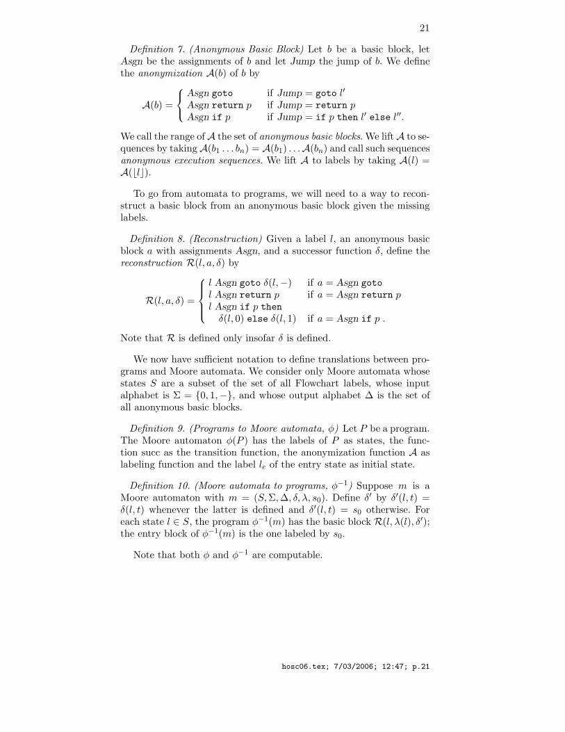
Definition 7. (Anonymous Basic Block) Let b be a basic block, letAsgn be the assignments of b and let Jump the jump of b. We definethe anonymization A(b) of b by
A(b) =
Asgn goto if Jump = goto l′
Asgn return p if Jump = return p
Asgn if p if Jump = if p then l′ else l′′.
We call the range ofA the set of anonymous basic blocks. We liftA to se-quences by takingA(b1 . . . bn) = A(b1) . . .A(bn) and call such sequencesanonymous execution sequences. We lift A to labels by taking A(l) =A(blc).
To go from automata to programs, we will need to a way to recon-struct a basic block from an anonymous basic block given the missinglabels.
Definition 8. (Reconstruction) Given a label l, an anonymous basicblock a with assignments Asgn, and a successor function δ, define thereconstruction R(l, a, δ) by
R(l, a, δ) =
l Asgn goto δ(l,−) if a = Asgn goto
l Asgn return p if a = Asgn return p
l Asgn if p then
δ(l, 0) else δ(l, 1) if a = Asgn if p .
Note that R is defined only insofar δ is defined.
We now have sufficient notation to define translations between pro-grams and Moore automata. We consider only Moore automata whosestates S are a subset of the set of all Flowchart labels, whose inputalphabet is Σ = {0, 1,−}, and whose output alphabet ∆ is the set ofall anonymous basic blocks.
Definition 9. (Programs to Moore automata, φ) Let P be a program.The Moore automaton φ(P ) has the labels of P as states, the func-tion succ as the transition function, the anonymization function A aslabeling function and the label le of the entry state as initial state.
Definition 10. (Moore automata to programs, φ−1) Suppose m is aMoore automaton with m = (S, Σ, ∆, δ, λ, s0). Define δ′ by δ′(l, t) =δ(l, t) whenever the latter is defined and δ′(l, t) = s0 otherwise. Foreach state l ∈ S, the program φ−1(m) has the basic block R(l, λ(l), δ′);the entry block of φ−1(m) is the one labeled by s0.
Note that both φ and φ−1 are computable.
hosc06.tex; 7/03/2006; 12:47; p.21
22
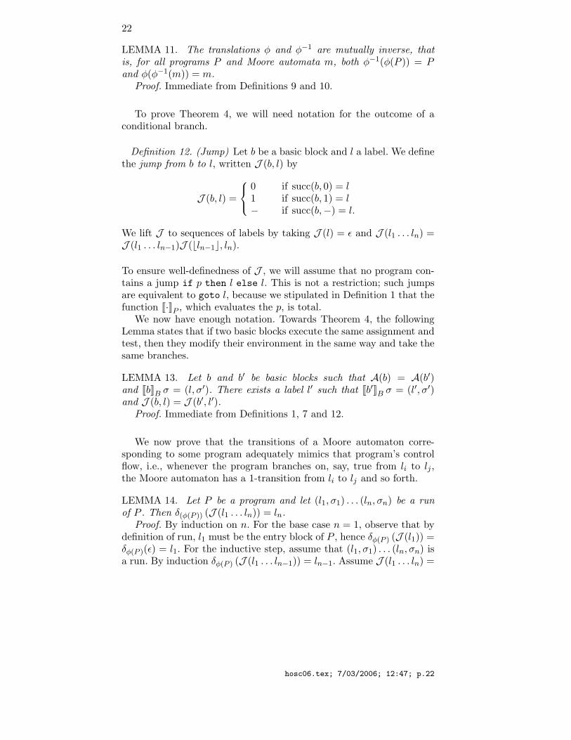
LEMMA 11. The translations φ and φ−1 are mutually inverse, thatis, for all programs P and Moore automata m, both φ−1(φ(P )) = P
and φ(φ−1(m)) = m.Proof. Immediate from Definitions 9 and 10.
To prove Theorem 4, we will need notation for the outcome of aconditional branch.
Definition 12. (Jump) Let b be a basic block and l a label. We definethe jump from b to l, written J (b, l) by
J (b, l) =
0 if succ(b, 0) = l
1 if succ(b, 1) = l
− if succ(b,−) = l.
We lift J to sequences of labels by taking J (l) = ε and J (l1 . . . ln) =J (l1 . . . ln−1)J (bln−1c, ln).
To ensure well-definedness of J , we will assume that no program con-tains a jump if p then l else l. This is not a restriction; such jumpsare equivalent to goto l, because we stipulated in Definition 1 that thefunction J·KP , which evaluates the p, is total.
We now have enough notation. Towards Theorem 4, the followingLemma states that if two basic blocks execute the same assignment andtest, then they modify their environment in the same way and take thesame branches.
LEMMA 13. Let b and b′ be basic blocks such that A(b) = A(b′)and JbKB σ = (l, σ′). There exists a label l′ such that Jb′KB σ = (l′, σ′)and J (b, l) = J (b′, l′).
Proof. Immediate from Definitions 1, 7 and 12.
We now prove that the transitions of a Moore automaton corre-sponding to some program adequately mimics that program’s controlflow, i.e., whenever the program branches on, say, true from li to lj ,the Moore automaton has a 1-transition from li to lj and so forth.
LEMMA 14. Let P be a program and let (l1, σ1) . . . (ln, σn) be a runof P . Then δ(φ(P )) (J (l1 . . . ln)) = ln.
Proof. By induction on n. For the base case n = 1, observe that bydefinition of run, l1 must be the entry block of P , hence δφ(P ) (J (l1)) =δφ(P )(ε) = l1. For the inductive step, assume that (l1, σ1) . . . (ln, σn) isa run. By induction δφ(P ) (J (l1 . . . ln−1)) = ln−1. Assume J (l1 . . . ln) =
hosc06.tex; 7/03/2006; 12:47; p.22

23
t1 . . . tn−1. We compute
δφ(P )(J (l1 . . . ln)) = δφ(P )(t1 . . . tn−1)
= δφ(P )(δφ(P )(t1 . . . tn−2), tn−1)
= δφ(P )(δφ(P )(J (l1 . . . ln−1)), tn−1)
= δφ(P )(ln−1, tn−1)
= ln.
The last equality follows from the definition of φ(P ).
It follows that each abstract execution sequence corresponds to theoutput of an automaton.
COROLLARY 15. Suppose that P is a program and that there is arun (l1, σ1) . . . (ln, σn) of P . Then A(l1 . . . ln) = Jφ(P )K (J (l1 . . . ln)).
Proof. It is sufficient to note that for 1 ≤ i ≤ n,
A(li) = A(blic) = λφ(P )(li) = λφ(P )(δφ(P )(J (l1 . . . li))).
We can now prove that equivalent Moore automata yield equivalentprograms.
LEMMA 16. Let m, m′ be equivalent Moore automata. Consider asequence σ1 . . . σn of environments.
1. There is a run (l1, σ1) . . . (ln, σn) of φ−1(m) if and only if there isa run (l′1, σ1) . . . (l′n, σn) of φ−1(m′).
2. If the above runs exist, they induce identical jump sequences andidentical abstract execution sequences:
J (l1 . . . ln) = J (l′1 . . . l′n)
A(l1 . . . ln) = A(l′1 . . . l′n)Proof. We proceed by induction on n. The base case is trivial. For
the inductive step, assume (l1, σ1) . . . (ln, σn) is a run of φ−1(m). Byinduction, there is a run (l′1, σ1) . . . (l′n−1, σn−1) such that
J (l1 . . . ln−1) = J (l′1 . . . l′n−1)
A(l1 . . . ln−1) = A(l′1 . . . l′n−1) (5)
Because (l1, σ1) . . . (ln, σn) is a run, Jbln−1cKB = (ln, σn). By (5) wehave A(ln−1) = A(l′n−1). We invoke Lemma 13 and find an l′n suchthat Jbl′n−1cKB
= (l′n, σn) and J (ln−1 ln) = J (l′n−1 ln). Hence there
hosc06.tex; 7/03/2006; 12:47; p.23

24
is a run (l′1, σ1) . . . (l′n, σn) of φ−1(m′) and J (l1 . . . ln) = J (l′1 . . . l′n).Using Corollary 15, we compute
A(l1 . . . ln) = Jφ(φ−1(m))K (J (l1 . . . ln))
= JmK (J (l1 . . . ln))
= Jm′K(
J (l′1 . . . l′n))
= Jφ(φ−1(m′))K(
J (l′1 . . . l′n))
= A(l′1 . . . l′n).
Finally, we have a proof of Theorem 4.
Proof of Theorem 4. Immediate from Lemma 16.
7. Discussion & Future Work
When one of our instrumented interpreters considers some basic blockfor transformation, it bases its decision on the particular execution pathtaken to reach that basic block. This accounts for the ease with whichwe have implemented otherwise complicated analyses and transforma-tions: Reasoning about a single execution path is inherently simplerthan reasoning about all possible execution paths.
However, this simplicity comes at a price. We are restricted to trans-formations that can be justified by inspecting only a single executionpath. Consider constant propagation (Muchnick, 1997). Offhand, con-stant propagation seems an easy transformation to implement by theinterpretive approach. Skip assignments x := c (where c is a constant),but do record x := c in a constant-propagation history; clear entries inthe constant-propagation history when variables are reassigned; thentry consulting the constant-propagation history before looking up vari-ables in the store. Presto, constants are propagated. However, considerthe effect of this implementation on the following fragment
if ... dox := 0;
elsex := 1;
end;
<more code>
Here, there are no opportunities for constant propagation, becausethe value of x at the <more code> program point is not staticallyknown. However, the suggested implementation would yield
hosc06.tex; 7/03/2006; 12:47; p.24

25
if ... do<more code, specialized to x := 0>
else<more code, specialized to x := 1>
end;
This transformation is correct, but much more aggressive than con-stant propagation — it more resembles partial evaluation. Tradition-ally, constant propagation implementations check whether an assign-ment x := c is available in all predecessors. When using the interpre-tive approach, we can work with only a single path of execution, so theinterpreter simply cannot inspect all the predecessors simultaneously.There seem to be no simple way to avoid this over-optimization. Weexpect that implementing copy propagation and dead-code eliminationwill prove similarly difficult. For the latter, there is the added compli-cation that liveness is a property of the future, whereas our interpreterscan only collect information about the past.
Future Work We see five major directions for future work.
1. Prove correctness of our implementations. Assuming correctness ofthe specializer, it is sufficient to prove our interpreters semanticallyequivalent. Such a proof would connect our results to ongoing workin provably correct compiler construction (Lacey et al., 2002; Lerneret al., 2003; Benton, 2004).
2. Explore more transformations. One challenge is to overcome theabove-mentioned difficulties with constant propagation, copy prop-agation and dead-code elimination. Another is to investigate lan-guages with pointers, requiring aliasing analysis.
3. Explore construction of optimizing compilers for domain-specificlanguages. Our specializer is standard except for rewinding, whichis merely a variant of Moore automaton minimization, so we canreasonably hope to feasibly construct such optimizing compilers byspecialization.
4. Integrate rewinding with specialization. Currently, we may pro-duce exponentially large residual programs only to cut them backdown with rewinding, incurring correspondingly exponential timeconsumption.
5. Formulate rewinding for functional languages, in particular higher-order functional languages.
hosc06.tex; 7/03/2006; 12:47; p.25

26
8. Acknowledgments
The author wishes to thank Torben Mogensen for useful discussions. Inaddition, the author gratefully acknowledges detailed and constructivecomments from Mads Sig Ager, Jakob Grue Simonsen, Lars Birkedaland the anonymous referees.
References
Benton, N.: 2004, ‘Simple relational correctness proofs for static analyses and pro-gram transformations’. In: POPL ’04: Proceedings of the 31st ACM SIGPLAN-
SIGACT symposium on Principles of programming languages. New York, NY,USA, pp. 14–25, ACM Press.
Debois, S.: 2004, ‘Imperative program optimization by partial evaluation’. In: PEPM
’04: Proceedings of the 2004 ACM SIGPLAN symposium on Partial evaluation
and semantics-based program manipulation. New York, NY, USA, pp. 113–122,ACM Press.
Denning, P. J., J. B. Dennis, and J. E. Qualitz: 1978, Machines, languages, and
computation. Prentice Hall.Gluck, R. and J. Jørgensen: 1994, ‘Generating optimizing specializers’. In: Proceed-
ings of the 1994 IEEE International Conference On Computer Languages. pp.183–194, IEEE Computer Society Press.
Gluck, R. and J. Jørgensen: 1994, ‘Generating transformers for deforestation and su-percompilation.’. In: SAS ’94: Proceedings of the 1st international Static analysis
symposium, Vol. 864 of Lecture Notes in Computer Science. pp. 432–448.Gomard, C. K. and N. D. Jones: 1991, ‘Compiler generation by partial evaluation:
a case study’. Structured Programming 12, 123–144.Hopcroft, J. E. and J. D. Ullman: 1979, Introduction to automata theory, languages
and computation. Addison–Wesley.Jones, N. D.: 2004, ‘Transformation by interpreter specialisation’. Science of
Computer Programming 52, 307–339.Jones, N. D., C. K. Gomard, and P. Sestoft: 1993, Partial evaluation and automatic
program generation. Prentice Hall.Lacey, D., N. D. Jones, E. V. Wyk, and C. C. Frederiksen: 2002, ‘Proving correctness
of compiler optimizations by temporal logic’. In: POPL ’02: Proceedings of
the 29th ACM SIGPLAN-SIGACT symposium on Principles of programming
languages. New York, NY, USA, pp. 283–294, ACM Press.Lerner, S., T. Millstein, and C. Chambers: 2003, ‘Automatically proving the correct-
ness of compiler optimizations’. In: PLDI ’03: Proceedings of the ACM SIGPLAN
2003 conference on Programming language design and implementation. NewYork, NY, USA, pp. 220–231, ACM Press.
Muchnick, S. S.: 1997, Advanced compiler design & implementation. MorganKaufmann Publishers.
Song, L., Y. Futamura, R. Gluck, and Z. Hu: 2000, ‘Loop quasi-invariance codemotion’. IEICE Transactions on Information and Systems E83-D(10), 1841–1850.
Sperber, M. and P. Thiemann: 1996, ‘Realistic compilation by partial evaluation’. In:PLDI ’96: Proceedings of the ACM SIGPLAN 1996 conference on Programming
language design and implementation. pp. 206–214, ACM Press.
hosc06.tex; 7/03/2006; 12:47; p.26

27
Thibault, S., C. Consel, J. L. Lawall, R. Marlet, and G. Muller: 2000, ‘Static anddynamic program compilation by interpreter specialization’. Higher-Order and
Symbolic Computation 13(3), 161–178.
Appendix
A. Macros
1 # Determine if elem is a an element of listmacro member (elem, list) :
tmp := list;4 while tmp != ‘() do
if hd tmp = elem doreturn ‘true;
end;8 tmp := tl tmp;
end;return ‘();
end12
# Assuming ’list’ is associative and has key ’key’, find the# corresponding value.macro lookup (key, list) :
16 tmp := list;while ‘true do
if hd (hd tmp) = key doreturn tl (hd tmp);
20 end;tmp := tl tmp;
end;return ‘(bad lookup);
24 end
# Reverse xs.macro reverse (xs) :
28 left := xs;right := ‘();
while left != ‘() do32 right := cons(hd left, right);
left := tl left;end;
36 return right;end
# Return first argument of the expression of assignment.40 macro param1Of (asgn) :
return hd (tl (tl asgn));end
44 # Assuming there is one, return second argument# of expression of assignment.macro param2Of (asgn) :
return hd (tl (tl (tl asgn)));48 end
# Construct assignment ’id := op (arg1, arg2)’.macro mkBinOpAsgn (id, op, param1, param2) :
52 return cons (id, cons (op,cons (param1,
cons (param2, ‘()))));end
hosc06.tex; 7/03/2006; 12:47; p.27

28
56# Return assignments target variable.macro def (asgn) :
return hd asgn;60 end
# Return list of identifiers referenced by assignment.macro use (asgn) :
64 ids := ‘();
if ‘id = hd (param1Of (asgn)) doids := cons (tl (param1Of (asgn)), ids);
68 end;
has2Args := tl (tl (tl asgn));if has2Args do
72 if ‘id = hd (param2Of (asgn)) doids := cons (tl (param2Of (asgn)), ids);
end;end;
76return ids;
end
Address for Offprints: IT University of CopenhagenRued Langgaardsvej 72300 Copenhagen SDenmark
hosc06.tex; 7/03/2006; 12:47; p.28