Embed Size (px)
Citation preview
Research Division Federal Reserve Bank of St. Louis Working Paper Series
Imperfect Competition and Sunspots
Pengfei Wang and
Yi Wen
Working Paper 2006-015A http://research.stlouisfed.org/wp/2006/2006-015.pdf
March 2006
FEDERAL RESERVE BANK OF ST. LOUIS Research Division
P.O. Box 442 St. Louis, MO 63166
______________________________________________________________________________________
The views expressed are those of the individual authors and do not necessarily reflect official positions of the Federal Reserve Bank of St. Louis, the Federal Reserve System, or the Board of Governors.
Federal Reserve Bank of St. Louis Working Papers are preliminary materials circulated to stimulate discussion and critical comment. References in publications to Federal Reserve Bank of St. Louis Working Papers (other than an acknowledgment that the writer has had access to unpublished material) should be cleared with the author or authors.
Imperfect Competition and Sunspots�
Pengfei WangDepartment of Economics
Cornell University
Yi WenResearch Department
Federal Reserve Bank of St. Louis
March 21, 2006
Abstract
This paper shows that imperfect competition can be a rich source of sunspots equilibria and
coordination failures. This is demonstrated in a dynamic general equilibrium model that has no
major distortions except imperfect competition. In the absence of fundamental shocks, the model
has a unique certainty (fundamental) equilibrium. But there is also a continuum of stochastic
(sunspots) equilibria that are not mere randomizations over fundamental equilibria. Markup is
always counter-cyclical in sunspots equilibria, which is consistent with empirical evidence. The
paper provides a justi�cation for exogenous variations over time in desired markups, which play
an important role as a source of cost-push shocks in the monetary policy literature. We show that
�uctuations driven by self-ful�lling expectations (or sunspots) look very similar to �uctuations
driven by technology shocks, and we prove that such �uctuations are welfare reducing.
Keywords: Sunspots, Self-ful�lling Expectations, Imperfect Competition, Imperfect Infor-
mation, Indeterminacy, Real Business Cycles, Marginal Costs, Counter-cyclical Markup.
JEL codes: E31, E32.
�We thank Jess Benhabib, Karl Shell, and seminar participates at Cornell University for comments, and JohnMcAdams for research assistance. The views expressed in the paper and any errors that may remain are the authors�alone. Correspondence: Yi Wen, Research Department, Federal Reserve Bank of St. Louis, St. Louis, MO, 63144.Phone: 314-444-8559. Fax: 314-444-8731. Email: [email protected].
1
1 Introduction
The work of Benhabib and Farmer (1994) has triggered a fast growing interest in studying expectations-
driven �uctuations. The major reason for this is that it makes quantitative analysis of the business-
cycle e¤ects of sunspots possible within the popular framework of Kydland and Prescott (1982).1
The Benhabib-Farmer model can be cast in two versions, one with production externalities or ex-
ternal increasing returns to scale, and one with monopolistic competition with internal increasing
returns to scale at the �rm level. Benhabib and Farmer show that if the returns to scale are su¢ -
ciently larger than one �either at the aggregate level or at the �rm level �then the steady state
of the model can become indeterminate and there can be in�nitely many equilibrium paths con-
verging to the same steady state. This multiplicity of equilibria can give rise to �uctuations driven
by purely extrinsic uncertainty (sunspots) or self-ful�lling expectations in this class of dynamic
stochastic general equilibrium (DSGE) models.
The Benhabib-Farmer model has been criticized by many as unrealistic because it relies on re-
turns to scale that are empirically implausible. Later developments in this literature, however, have
been able to bring the degree of returns-to-scale required for indeterminacy down to an empirically
plausible range (see, e.g., Benhabib and Farmer, 1996, and Wen, 1998a). Despite this, indetermi-
nacy in these types of models is still sensitive to the values of other structural parameters, such as
the output elasticity of capital and the elasticity of labor supply (e.g., it requires the elasticity of
labor supply to be close to in�nity). This is so because these structural parameters and returns to
scale jointly a¤ect the eigenvalues of the model. Local indeterminacy would not arise in this class
of models, for example, if there were adjustment costs in capital or labor (see Georges 1995, and
Wen 1998b).2 Due to these restrictions on structural parameters in the Benhabib-Farmer model,
the Keynesian idea of �uctuations driven by animal spirits (or sunspots) has not gained su¢ cient
popularity in the real business cycle (RBC) circle, where technology shocks are still viewed as the
dominate force behind economic �uctuations.
This paper shows that there exists an entirely di¤erent source of sunspots equilibria in the
Benhabib-Farmer model. This new source of sunspots equilibria can arise naturally in standard
dynamic stochastic general equilibrium models, and is robust to the choice of parameter values in
production technologies and utility functions. In other words, we show that in order to generate
sunspots equilibria in the class of in�nite-horizon, calibrated RBC (or DSGE) models, returns to
scale are completely irrelevant and unnecessary. The key condition required for sunspots equilibria,
1For a literature review, see Benhabib and Farmer (1999). For early contributions to the sunspots literature, seeShell (1977), Azariadis (1981), Cass and Shell (1983), and Woodford (1986), among others.
2A common feature of the requirements on the parameter values for indeterminacy is that they must facilitategreater �exibility of factor mobility and enhance the temporal/intertemporal substitutability of factors, so that theshort-run returns to labor can exceed one. Adjustment costs tend to work against these e¤ects. Gali (1994) presentsa di¤erent model that does not rely on increasing returns to scale to generate local indeterminacy. However, theparameter region of indeterminacy in Gali�s model is also sensitive to the values of structural parameters.
2
or for expectations to be self-ful�lling, is imperfect competition with di¤erentiated products. As
is shown by Blanchard and Kiyotaki (1987), product di¤erentiation can lead to externalities of its
own �demand externalities.3 We show that this type of demand externality is a rich source of
sunspots equilibria under imperfect competition. Furthermore, we show that �uctuations driven
by sunspots behave very much like those driven by technology shocks.4
The nature of the sunspots equilibria arising under the demand externalities di¤ers from that
arising under the production externalities studied by Benhabib and Farmer in two important as-
pects: 1) sunspots are global instead of local, hence they have nothing to do with the topological
properties of the steady state, as they do not require the steady state to be a sink as in Benhabib
and Farmer (1994); 2) sunspots equilibria under our speci�cation are not based on mere random-
izations over fundamental equilibria, in sharp contrast to the sunspots equilibria studied in the
literature using the Benhabib-Farmer framework.5
Because of property (1), sunspots are more pervasive than is currently known since multiplicity
of equilibria no longer depends on the structural parameters that a¤ect the eigenvalues of the
model, as in the Benhabib-Farmer model. Consequently, the multiplicity is robust �any economic
environment featuring the Dixit-Stiglitz type of imperfect competition is a potential source of
sunspots and hence can be subject to sunspots-driven �uctuations, regardless of utility functions and
production technologies. Because of property (2), sunspots equilibria can arise in a dynamic model
with a unique saddle-path fundamental equilibrium. This property is important because it makes
the classic Keynesian notion of animal spirits more convincing. In this regard, our �nding extends
the classical analysis of sunspots equilibria by Cass and Shell (1983) into a new dimension �the
analysis of sunspots-driven �uctuations can be conducted in standard, in�nite-horizon RBC/DSGE
models with constant returns to scale and a unique fundamental equilibrium.
The intuition behind our �ndings is simple. When there are multiple �rms in the economy and
each �rm�s optimal action depends on other �rms�actions, there exists strategic complementar-
ity among �rms�behaviors. Such strategic complementarity can lead to multiple equilibria and
coordination failures, as is shown by Cooper and John (1988). Strategic complementarity arises
naturally in the Dixit-Stiglitz type of imperfect competition models due to the imperfect substi-
tutability among the intermediate goods produced by monopolistic �rms, which gives rise to an
endogenous demand externality (as argued by Blanchard and Kiyotaki, 1987). The externality is
endogenous because it is not imposed from outside as in the Benhabib-Farmer framework. Since
3This refers to the case where demand for an individual �rm�s output depends on demand for other �rms�outputdue to imperfect substitutability among �rms�output.
4Since perfect competition can be represented as a limiting case of imperfect competition, our results also applyto models with perfect (or near-perfect) competition, as in the set up of Alvarez and Lucas (2004). See Proposition1 in the text.
5See, e.g., Farmer and Guo (1994).
3
many representative-agent DSGE models can be easily mapped into models with decentralized de-
cision making featuring the Dixit-Stiglitz type of competition among �rms,6 sunspots equilibria
can therefore exist in a wide class of real business cycle models as well as in Keynesian sticky-price
models, including the monopolistic competition version of the Benhabib-Farmer model (regardless
of the production externalities or increasing returns to scale).
The demand externality is a necessary but not su¢ cient condition for the rise of sunspots
equilibria in models with imperfect competition. Another crucial condition needed for sunspots
equilibria is imperfect information. That is, individual monopolistic �rms make price decisions
without knowing the level of aggregate demand �because they do not know how the other �rms
will set their prices. Hence, �rms must each form expectations about the aggregate conditions of
the economy when setting prices. Such expectations can be self-ful�lling because of the strategic
complementarities among �rms�actions. Monopolistic competition has been studied extensively
in the literature. The reason that the possibility of sunspots equilibria has gone unnoticed in the
literature is that standard DSGE models of imperfect competition always implicitly assume perfect
information �that each �rm knows precisely the level of aggregate demand when setting its prices.
This assumption of perfect information rules out multiple-sunspots Nash equilibria. However, if
�rms each choose a price (taking as given the prices set by other �rms) and quantities of demand
are subsequently determined at these prices, then it is more natural to assume that prices are set
based on expected demand, not on realized demand.7
Our �ndings can be viewed as a natural extension of the analysis of Cooper and John (1988). Our
main contribution in this paper, compared to Cooper and John, is to show the existence of multiple
equilibria in calibrated, in�nite horizon, DSGE models. This class of models is the workhorse
of theoretical and applied macroeconomics in the study of business cycles and monetary policy.
Although the Dixit-Stiglitz (1977) imperfect competition model belongs to the class of models
considered by Cooper and John in a broad sense, they do not analyze the conditions of multiple
equilibria in a dynamic-general-equilibrium framework. The theorems proposed by Cooper and
John for multiple equilibria are therefore insu¢ cient for characterizing the existence of multiple
equilibria in the class of dynamic models we study. For example, the models we study meet the
conditions for multiple fundamental equilibria speci�ed by Cooper and John, yet we show that the
fundamental equilibrium is nonetheless unique in our models. The only type of sunspots equilibria
that can arise in the models studied by Cooper and John are randomizations over fundamental
equilibria, whereas sunspots equilibria studied in this paper are not mere randomizations over
fundamental equilibria. As such, Cooper and John do not prove the existence of multiple equilibria
6See Proposition 2 in this paper.7We are not the �rst to link imperfect competition and imperfect information to sunspots equilibria. For the early
literature, see Peck and Shell (1991), Woodford (1991), and Gali (1994), among others.
4
in the class of dynamic models we study and do not show how to construct stochastic sunspots
equilibria in an environment where there is a unique fundamental equilibrium.8
Our �ndings provide an interesting contribution to the literature because the Dixit-Stiglitz
imperfect competition framework is widely used in economic analysis. The fast growing New Key-
nesian sticky-price literature is just one of the many noticeable areas that relies on this framework
for business-cycle studies and monetary policy analyses. Yet this literature has been assuming
unique equilibrium all the way along, while in fact there may be multiple equilibria and severe
coordination-failure problems in such models. In addition, since the most celebrated neoclassical
business-cycle model of Kydland and Prescott (1982) can be cast as a limiting case of the Dixit-
Stiglitz imperfect competition model, and since �uctuations driven by technology shocks look sim-
ilar to those driven by sunspots shocks, business cycles in general may not be the optimal response
of the market economy to exogenous shocks (as accepted by the RBC literature), but instead may
be �uctuations driven by self-ful�lling expectations and coordination failures. Such �uctuations are
highly ine¢ cient, as we prove in this paper. Hence, designing policies that can dampen �uctuations
and prevent the coordination failures is central to business cycle studies, and such analysis can be
conducted using the framework we provide in this paper.
Another important contribution of the paper is that it provides a justi�cation for exogenous
variations over time in desired markups, which play an important role as a source of cost-push
shocks in the monetary policy literature (see, e.g., Clarida, Gali, and Gertler, 1999 and 2001;
Walsh, 1999; Steinsson, 2003; Ravenna and Walsh, 2004; and Lane, Devereux, and Xu, 2005,
among many others). This literature shows that there exist in�ation-output trade-o¤s for the
design of optimal monetary policies when there are independent shocks to �rms�marginal costs
or markups. To justify autonomous shifts in �rms�marginal costs, the literature has been relying
mainly on the ad hoc assumption that the elasticity of substitution across intermediate inputs in the
�nal-good production technology is random. This paper shows that marginal costs can be driven
by purely extrinsic uncertainty or sunspots without changes in the fundamentals, hence providing
a justi�cation for the independent random movements in marginal costs.
The rest of the paper is organized as follows. Section 2 presents a general equilibrium model
of imperfect competition and proves the uniqueness of the fundamental equilibrium in the model.
Section 2 shows the existence of sunspots equilibria, and that �uctuations driven by sunspots
behave similar to those driven by technology shocks. Section 4 studies the welfare properties of
8A fundamental equilibrium is an equilibrium in the absence of extrinsic uncertainty. Blanchard and Kiyotakiare able to construct multiple fundamental equilibria in a model similar to ours under the additional assumption ofmenu costs. Kiyotaki (1988) also uses a similar set up with Dixit-Stiglitz imperfect competition to generate multiplefundamental equilibria in a two-period dynamic setting. However, Kiyotaki requires increasing-returns-to-scale as anecessary condition for multiple equilibria. An important distinction between our paper and this literature is that thetype of sunspots equilibria we construct are not mere randomizations over fundamental equilibria. There is alwaysa unique fundamental equilibrium in our model and we do not rely on menu costs or increasing returns to scale toconstruct sunspots equilibria.
5
sunspots equilibria and proves that sunspots-driven �uctuations are ine¢ cient. Section 5 studies
the robustness of sunspots equilibria in models with money and sticky prices. Finally, Section 6
concludes the paper.
2 The Benchmark Model
2.1 Firms
Suppose there is a continuum of intermediate good producers indexed by i �[0; 1]; with each pro-
ducing a single di¤erentiated good Y (i). The price of Y (i) is denoted P (i). These intermediate
goods are used as inputs to produce a �nal good according to the technology,
Y =
0@ 1Z0
Y (i)��1� (i)di
1A�
��1
; (1)
where � > 1 measures the elasticity of substitution among the intermediate goods. The �nal good
industry is assumed to be perfectly competitive. The price of the �nal good, P , is normalized to
one. Pro�t maximization by the �nal good producer yields the demand function for intermediate
goods:
Y (i) = P (i)��Y: (2)
Notice that the demand for good i depends not only on the relative price of the good, but also
on the aggregate demand Y . There are thus demand externalities in the model as pointed out by
Blanchard and Kiyotaki (1987). It is important to emphasize that the demand externality arises
endogenously within the model due to the complementarity of production factors (intermediate
goods) in the �nal good industry, as opposed to being exogenously imposed from outside as in
the case of the production externalities assumed in the Benhabib-Farmer model. Substituting
the demand functions into the �nal-good production function (1) gives the aggregate price index,
P (= 1) =�R 10 P (i)
1��di�1=(1��)
:
The production technology for intermediate goods has constant returns to scale and is given by
Y (i) = K(i)�N(i)1��: (3)
Intermediate good producers have monopoly power in the output market but are perfectly compet-
itive in the factor markets. Given the production technology, the cost function of an intermediate
good �rm can be derived by solving a cost-minimization problem, min fWN(i) +RK(i)g, subject
toK(i)�N(i)1�� � Y (i), whereW and R denote the real wage and the real rental rate, respectively.
6
Letting � denote the marginal cost (which is the Lagrangian multiplier for the constraint of the
�rm�s cost minimization problem), we have the factor demand functions for labor and capital for
each �rm i: W = (1 � �)�(i) Y (i)N(i) and R = ��(i) Y (i)K(i) : Combining these factor demand functions
and the production function (1), we have � =�W1��
�1�� �R�
��as the unit cost function of the �rm.
This shows that marginal cost is the same across all �rms in the model. Since � is the shadow
cost of increasing �rm i�s output by one unit, in general equilibrium its correlation with aggregate
demand is nonnegative: cov(�; Y ) � 0.A key feature of the model is that intermediate good �rms each choose a price while taking
as given the prices set by other �rms, with quantities being then determined by demand at these
prices in general equilibrium. This sequential feature of the model permits imperfect information.
This is so because, in each period t, intermediate good �rms must set prices without knowing the
aggregate economic conditions (such as aggregate demand) that may prevail in period t. These
aggregate economic conditions depend crucially on the actions of the other �rms over which an
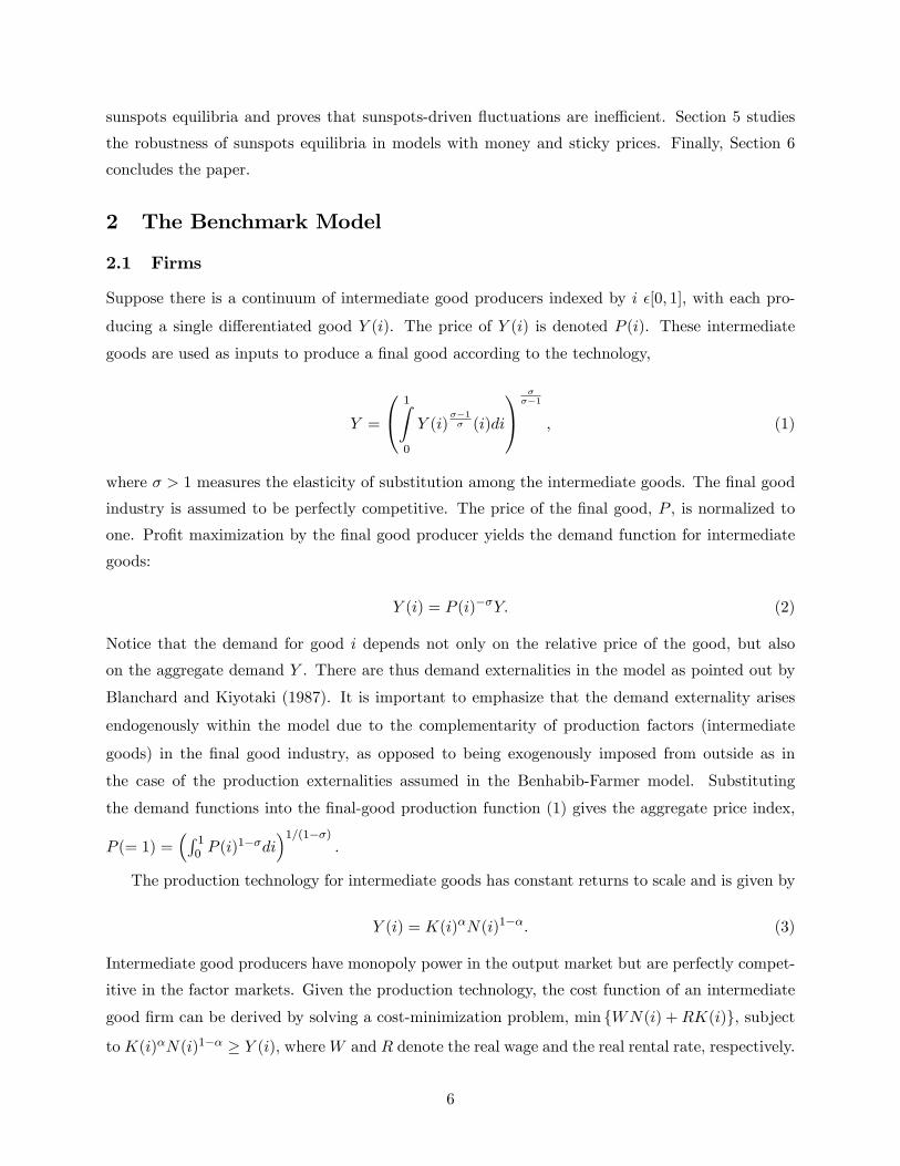
individual �rm has no in�uence. Figure 1 illustrates the sequence of events in the model economy.
)(ipt
t 1+t
Sunspots },,,,,,{ 1 ttttttt RWKNCY φ+
)(1 ipt+
Fig. 1. Timing of Sunspots.
De�ne ~t as the information set available to price setting �rms in period t; which includes the
entire history of the economy up to period t except the realizations of sunspots (if any) in period
t. Denote t as the information set that includes ~t and any realization of sunspots in period t.
Thus we have t � ~t � t�1. Since we do not consider fundamental shocks in this paper, we have
7
~t = t�1. Extension of the analysis to including fundamental shocks is straightforward.9 Based
on this de�nition of information sets, each individual �rm i chooses price Pt(i) in the beginning of
period t to maximize expected pro�ts by solving
maxEt�1 f(Pt(i)� �t)Yt(i)g ; (4)
subject to the downward sloping demand function, Y (i) =�P (i)P
���Y , where Et�1 denotes expec-
tations conditioned on the information set t�1(= ~t).10
The optimal monopolistic price is given by
Pt(i) =�
� � 1Et�1 (�tYt)
Et�1Yt; (5)
where ���1 � 1. In the limiting case where � !1, the model converges to a perfectly competitive
economy. Our analysis of sunspots equilibria is independent of �, hence it applies equally to
perfectly (or near-perfectly) competitive economies where �rms set prices equal to marginal cost
with zero markup in the steady-state. The optimal pricing rule shows that an individual �rm sets
prices according the expected aggregate cost-to-revenue ratio, where both the �rm�s revenue and its
costs depend on expected aggregate demand. Equation (5) indicates a potential source of multiple
Nash-sunspots equilibria. To see this, suppose we close the model by specifying an aggregate labor
supply curve, Nt = N(Wt); which implies that in general equilibrium the aggregate output is a
function of the marginal cost (since the real wage depends on the marginal cost), Yt = Y (�t;Kt):
In a symmetric equilibrium, P (i) = P = 1, and assuming that the aggregate capital stock is known
to �rms at the moment of price setting, Equation (1) becomes
�
� � 1Et�1 [�tY (�t;K)]
Et�1Y (�t;K)= 1: (50)
This equation may permit sunspots solutions for the marginal cost, �t(K), which are not mere ran-
domizations of fundamental equilibria. Suppose there is no extrinsic uncertainty (i.e., there is per-
fect information about the level of aggregate demand, Y ); then Equation (50) implies ���1Et�1�t =
1. Since by assumption Y (�t;K) is known to the �rms at the time of price setting, the marginal
cost �t must also be known to the �rms in period t based on the information set t�1. Hence a
9Notice that our de�nition of information sets does not necessarily imply sticky prices. Prices can be allowedto respond immediately to any fundamental shocks in the model. That is, the information set ~t can includefundamental shocks realized in period t. As such, prices can respond to money shocks one for one. However, withrespect to sunspots shocks, the price setting behavior in our model is in spirit similar to the sticky price literature(e.g., Yun 1996) and the sticky information literature (e.g., Mankiw and Reis, 2002). In reality, it is often the casethat �rms set prices before observing demand and demand decisions are often made based on observed prices.10The reason that an individual �rm needs to form expectations when maximizing pro�ts is because the pro�ts
depend on the aggregate demand, which in turn depends on the prices set by other �rms in the economy.
8
constant marginal cost, � = ��1� ; is the only fundamental-equilibrium solution to Equation (50).
Given �, aggregate demand is then fully determined in period t at the level Y (��1� ;K). However,
with extrinsic uncertainty or imperfect information, a random process �t could also constitute a
solution for Equation (50). To see this, let Y be a separable function, Y (�;K) = g(�)f(K). Then
Equation (50) becomes ���1
E[�g(�)]Eg(�) = 1. This implies Eg(�)
�E�� ��1
�
�= �cov(�; g(�)) � 0.11
Hence, any random process f�tg satisfying E� � ��1� may constitute an equilibrium in which the
level of aggregate demand is given by Y (�t;K).
The source of the stochastic multiple equilibria for the marginal cost comes from the fact
that each individual �rm does not know how the other �rms will behave, and hence must form
expectations for the status of the aggregate economy when making price decisions. Due to the
endogenous demand externalities among �rms� actions, such expectations can be self-ful�lling.
This possibility is analyzed in more detail in what follows.
2.2 Households
Suppose there is a representative household in the economy, whose objective is to maximize its
lifetime utility,
U = E0
1Xt=0
�tu(ct; lt); 0 < � < 1; (6)
where c and l are the household�s consumption and leisure time, u(�; �) is an increasing and concaveperiod-utility function, and � is the time discount rate. The household is endowed with one unit
of time in each period, so its labor supply in each period is n = 1 � l. The household�s budgetconstraint in period t is given by
ct + kt+1 =Wtnt + (1 +Rt � �)kt +Dt; (7)
where kt is the household�s existing stock of capital, which depreciates at the rate � 2 (0; 1],
Wtnt + Rtkt is the household�s real income from labor and renting capital to �rms, and Dt is the
real pro�ts distributed from �rms.
2.3 General Equilibrium
A general equilibrium is de�ned as the set of prices and quantities, fW;R; �; P (i); Y (i); N(i);K(i); c; k; ng; such that �rms maximize pro�ts and the household maximizes utility subject to their11The marginal cost � also measures the e¢ ciency of the aggregate economy. A higher value of � implies less
monopolistic distortion to the economy and thus more output. Hence cov(�; Y ) � 0; or likewise @Y@�� 0.
9
respective technological and budget constraints, and all markets clear:
nt = Nt �ZNt(i)di (8)
kt = Kt �ZKt(i)di (9)
ct +Kt+1 � (1� �)Kt = Yt: (10)
We analyze symmetric equilibria where all intermediate good �rms choose the same prices and
produce the same equilibrium quantities. The sunspots equilibria we construct are pure Nash
equilibria.
Since all �rms face the same problem in each period, they set the same prices according to (5).
Hence, in a symmetric equilibrium, we have P (i) = 1 and ���1
Et�1(�tYt)Et�1Yt
= 1: Given that Pt(i) = 1
in equilibrium, the supply function for �rm i becomes
Yt(i) = Yt; (11)
which is the same across all �rms. That is, in equilibrium, how much each individual �rm produces
depends on how much the rest of the economy produces. This type of externality can give rise to
multiple equilibria because each �rm may opt to produce more if they all expect that the other
�rms will produce more. That is, expectations can be self-ful�lling.
However, as will become clear shortly, the demand externality is a necessary but not su¢ cient
condition for multiple equilibria in the dynamic general equilibrium model. In order to obtain
multiple equilibria in the model, we need another key element � imperfect information. That
is, �rms determine prices without knowing the prices set by other �rms and hence must form
expectations for the equilibrium marginal cost and aggregate demand, which serve as indicators for
the aggregate economic conditions.
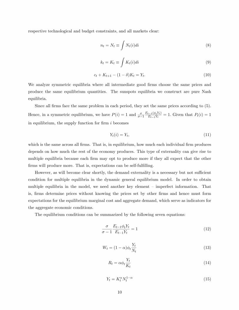
The equilibrium conditions can be summarized by the following seven equations:
�
� � 1Et�1�tYtEt�1Yt
= 1 (12)
Wt = (1� �)�tYtNt
(13)
Rt = ��tYtKt
(14)
Yt = K�t N
1��t (15)
10
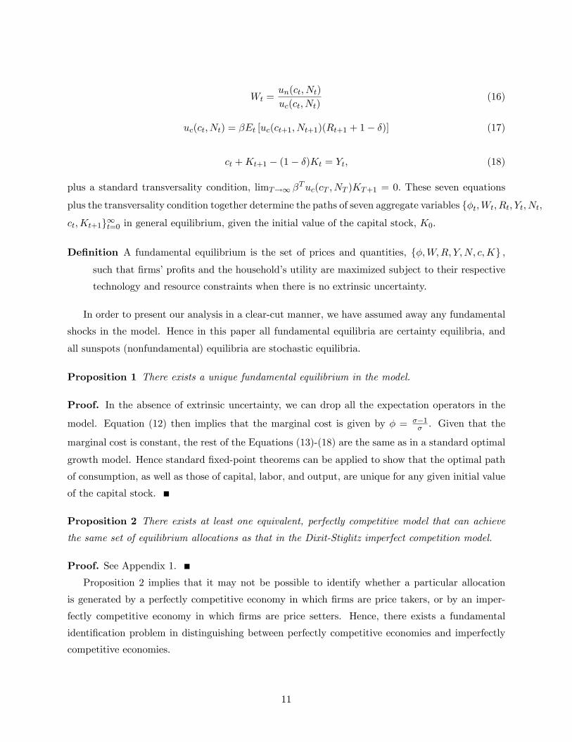
Wt =un(ct; Nt)
uc(ct; Nt)(16)
uc(ct; Nt) = �Et [uc(ct+1; Nt+1)(Rt+1 + 1� �)] (17)
ct +Kt+1 � (1� �)Kt = Yt; (18)
plus a standard transversality condition, limT!1 �Tuc(cT ; NT )KT+1 = 0: These seven equations
plus the transversality condition together determine the paths of seven aggregate variables f�t;Wt; Rt; Yt; Nt;
ct;Kt+1g1t=0 in general equilibrium, given the initial value of the capital stock, K0.
De�nition A fundamental equilibrium is the set of prices and quantities, f�;W;R; Y;N; c;Kg ;such that �rms�pro�ts and the household�s utility are maximized subject to their respective
technology and resource constraints when there is no extrinsic uncertainty.
In order to present our analysis in a clear-cut manner, we have assumed away any fundamental
shocks in the model. Hence in this paper all fundamental equilibria are certainty equilibria, and
all sunspots (nonfundamental) equilibria are stochastic equilibria.
Proposition 1 There exists a unique fundamental equilibrium in the model.
Proof. In the absence of extrinsic uncertainty, we can drop all the expectation operators in the
model. Equation (12) then implies that the marginal cost is given by � = ��1� . Given that the
marginal cost is constant, the rest of the Equations (13)-(18) are the same as in a standard optimal
growth model. Hence standard �xed-point theorems can be applied to show that the optimal path
of consumption, as well as those of capital, labor, and output, are unique for any given initial value
of the capital stock.
Proposition 2 There exists at least one equivalent, perfectly competitive model that can achieve
the same set of equilibrium allocations as that in the Dixit-Stiglitz imperfect competition model.
Proof. See Appendix 1.
Proposition 2 implies that it may not be possible to identify whether a particular allocation
is generated by a perfectly competitive economy in which �rms are price takers, or by an imper-
fectly competitive economy in which �rms are price setters. Hence, there exists a fundamental
identi�cation problem in distinguishing between perfectly competitive economies and imperfectly
competitive economies.
11
3 Sunspots Equilibria
3.1 Without Capital
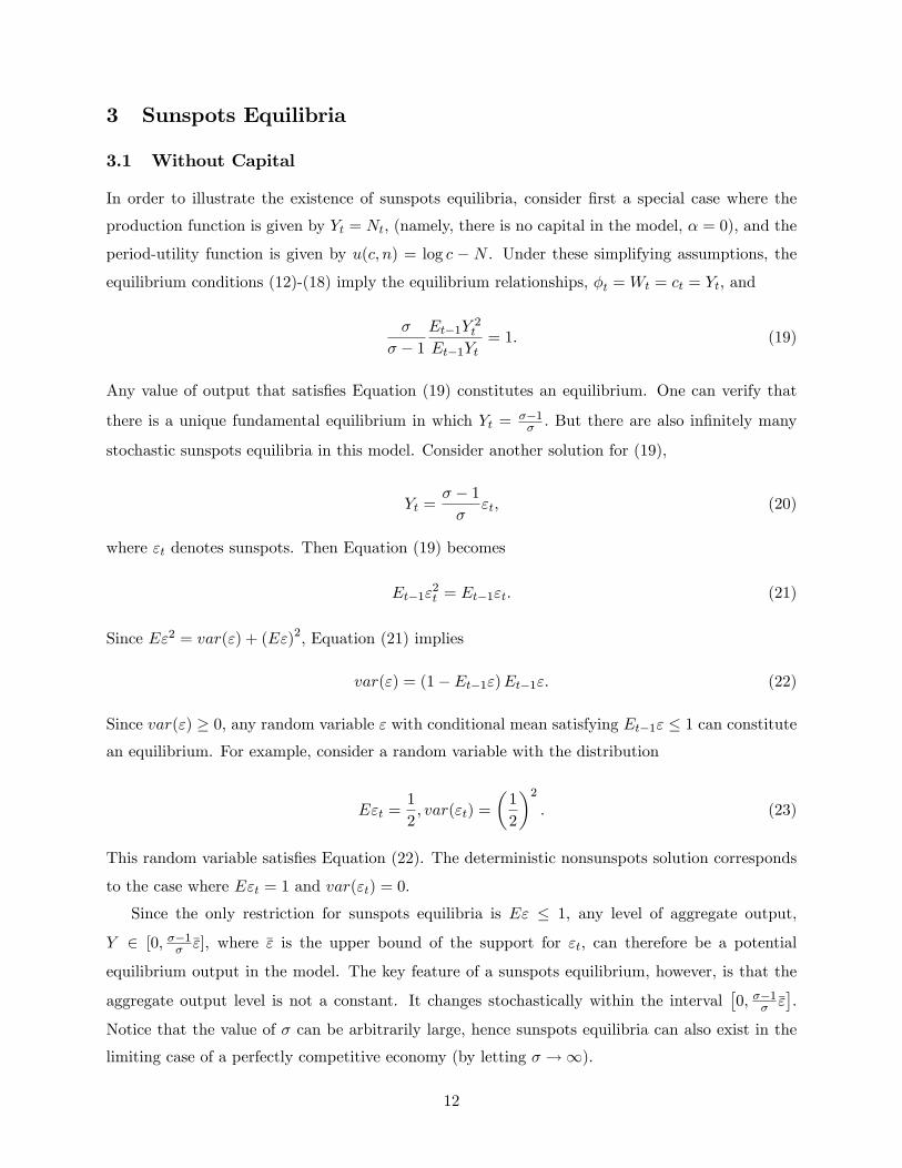
In order to illustrate the existence of sunspots equilibria, consider �rst a special case where the
production function is given by Yt = Nt; (namely, there is no capital in the model, � = 0), and the
period-utility function is given by u(c; n) = log c � N . Under these simplifying assumptions, theequilibrium conditions (12)-(18) imply the equilibrium relationships, �t =Wt = ct = Yt; and
�
� � 1Et�1Y 2tEt�1Yt
= 1: (19)
Any value of output that satis�es Equation (19) constitutes an equilibrium. One can verify that
there is a unique fundamental equilibrium in which Yt = ��1� : But there are also in�nitely many
stochastic sunspots equilibria in this model. Consider another solution for (19),
Yt =� � 1�
"t; (20)
where "t denotes sunspots. Then Equation (19) becomes
Et�1"2t = Et�1"t: (21)
Since E"2 = var(") + (E")2, Equation (21) implies
var(") = (1� Et�1")Et�1": (22)
Since var(") � 0, any random variable " with conditional mean satisfying Et�1" � 1 can constitutean equilibrium. For example, consider a random variable with the distribution
E"t =1
2; var("t) =
�1
2
�2: (23)
This random variable satis�es Equation (22). The deterministic nonsunspots solution corresponds
to the case where E"t = 1 and var("t) = 0.
Since the only restriction for sunspots equilibria is E" � 1, any level of aggregate output,
Y 2 [0; ��1� �"], where �" is the upper bound of the support for "t; can therefore be a potential
equilibrium output in the model. The key feature of a sunspots equilibrium, however, is that the
aggregate output level is not a constant. It changes stochastically within the interval�0; ��1� �"
�.
Notice that the value of � can be arbitrarily large, hence sunspots equilibria can also exist in the
limiting case of a perfectly competitive economy (by letting � !1).
12
These equilibria are clearly Pareto ranked since the household�s utility function depends monoton-
ically on the aggregate output Y . The maximum expected output is ��1� , which can be achieved
only in the certainty (nonsunspots) equilibrium (recall that E" = 1 implies var(") = 0 by Equation
22). As such, sunspots are welfare reducing in this simpli�ed model. A general statement on the
welfare properties of sunspots will be provided later.
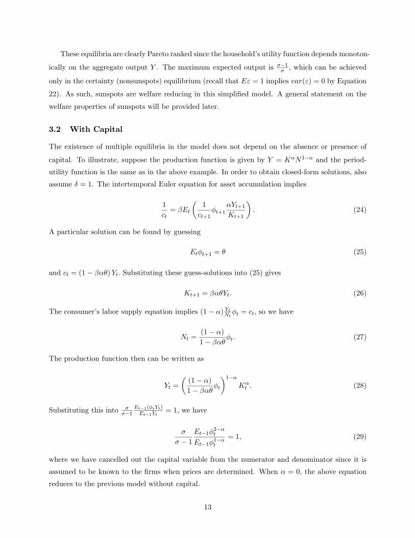
3.2 With Capital
The existence of multiple equilibria in the model does not depend on the absence or presence of
capital. To illustrate, suppose the production function is given by Y = K�N1�� and the period-
utility function is the same as in the above example. In order to obtain closed-form solutions, also
assume � = 1. The intertemporal Euler equation for asset accumulation implies
1
ct= �Et
�1
ct+1�t+1
�Yt+1Kt+1
�: (24)
A particular solution can be found by guessing
Et�t+1 = � (25)
and ct = (1� ���)Yt: Substituting these guess-solutions into (25) gives
Kt+1 = ���Yt: (26)
The consumer�s labor supply equation implies (1� �) YtNt�t = ct, so we have
Nt =(1� �)1� ����t: (27)
The production function then can be written as
Yt =
�(1� �)1� ����t
�1��K�t : (28)
Substituting this into ���1
Et�1(�tYt)Et�1Yt
= 1, we have
�
� � 1Et�1�
2��t
Et�1�1��t
= 1; (29)
where we have cancelled out the capital variable from the numerator and denominator since it is
assumed to be known to the �rms when prices are determined. When � = 0, the above equation
reduces to the previous model without capital.
13
A constant marginal cost, � = ��1� , is the only fundamental equilibrium in the model. There
are also many stochastic sunspots equilibria in the model. Any dynamic process of the marginal
cost satisfying (25) and (29) constitutes a rational-expectations sunspots equilibrium. For example,
a solution that takes the form
�t =� � 1�
"t; (30)
with the sunspots variable " satisfying
Et�1"2��t = Et�1"
1��t (31)
and Et�1"t equalling a constant, constitutes an equilibrium. For example, the distribution
"t =
8<:0 with probability p
1 with probability 1� p(32)
will satisfy these conditions for any p 2 [0; 1]. In this case, the equilibrium value of � is given
by � = ��1� (1 � p): Notice that the sunspots shock to the marginal cost, ", represents a shock
to the expected aggregate demand because the marginal cost is the Lagrangian multiplier for the
constraint, K�N1�� � Y , in the cost-minimization problem of the �rms. The marginal cost
increases if and only if the demand increases.
Since p 2 [0; 1], we have just constructed a continuum of sunspots equilibria that are not mere
randomizations over fundamental equilibria. Each value of p 2 (0; 1) corresponds to one particularstochastic sunspots equilibrium. The certainty equilibrium corresponds to the case of p = 0. There
are also other types of sunspots equilibria in the model. For example, we can assume that the
probability p is a time-varying random variable with a constant mean (�p 2 (0; 1)),
pt = �p+ �t; (33)
where �t is a stationary mean-reverting random process with zero mean and support [��p; 1� �p].Since �t can be serially correlated in a complicated manner, the sunspots equilibria can have very
complicated dynamic properties.
It is important to emphasize that the type of sunspots equilibria in the model is global and
robust. It is global because it is not based on a local linearization, hence it is independent of the
topological properties of the steady state. It is robust because it is independent of the model�s
structural parameters, as opposed to the case analyzed by Benhabib and Farmer. The results hold
regardless of the utility functions and the output elasticities of capital and labor. They hold even in
the limiting case of (near) perfect competition (i.e., when � !1). The real business cycle model
14
of Kydland and Prescott (1982) can be cast into this framework by properly decentralizing it in a
way similar to Benhabib and Farmer (1994) and then taking the limit, � !1.
3.3 A Calibration Exercise
Let the period-utility function be given by u(c;N) = log(c) � anN1+
1+ . When � 6= 1 and 6= 0,
closed-form solutions are not obtainable, but approximate solutions can be found by linearizing
the model around a deterministic steady state where the long-run value of the marginal cost is a
constant, �� = ��1� . Denote a circum�ex variable as xt � logXt � log �X, where �X denotes the
long-run value of X for a deterministic steady state. Log-linearizing the equilibrium conditions
(12)-(18) around the deterministic steady state, after substituting out fw; r; yg we have
Et�1�t = 0 (34)
(�+ ) nt = �t + �kt � ct (35)
ct = Etct+1 � (1� �(1� �))Eth�t+1 + (�� 1) kt+1 + (1� �)nt+1
i(36)
(1� si)ct + si�1
�kt+1 �
1� ��kt
�= �kt + (1� �)nt; (37)
where si = ����
1��(1��) is the long-run saving rate in the deterministic steady state.
Notice that the model is reduced to a standard RBC model without sunspots if �t = 0 for all t
(i.e., if �t is constant). However, �t does not have to be constant. Firms�price setting behavior only
implies that the expected value of �t is constant in this linearized version of the model (Equation
34). Thus, the above system clearly suggests that we can treat the marginal cost �t as an exogenous
forcing variable of the model economy. Let �t be an i:i:d: random variable with mean zero; the
above system of equations can be reduced to
Et
�kt+1ct+1
�=M
�ktct
�+ ��t: (38)
The saddle-path property of the model implies that the coe¢ cient matrix M has exactly one
explosive eigenvalue and one stable eigenvalue. Hence the optimal consumption level can be solved
by the method of Blanchard and Kahn (1980) to get the saddle-path solution, ct = 1kt+ 2�t; where
15
f 1; 2g denote coe¢ cients. Since the marginal cost �t is indeterminate, any i:i:d: representation
of �t with zero conditional mean can constitute an equilibrium path for consumption.12
Following the existing RBC literature (e.g., Kydland and Prescott, 1982), we calibrate the
model as follows: the time period is a quarter, the time discounting factor � = 0:99, the rate of
depreciation � = 0:025, the inverse labor supply elasticity = 0:25, and capital�s share in aggregate
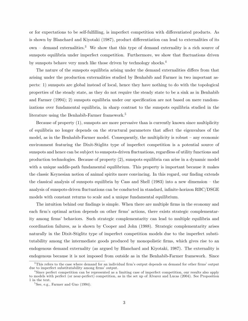
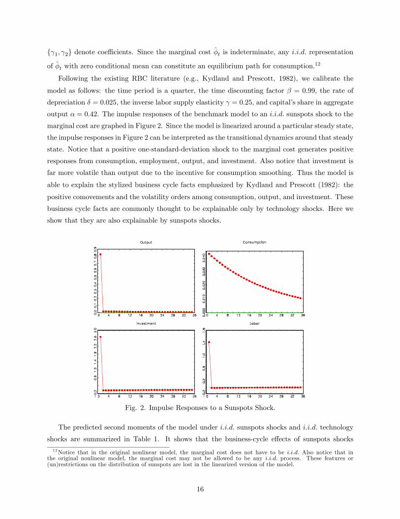
output � = 0:42. The impulse responses of the benchmark model to an i:i:d: sunspots shock to the
marginal cost are graphed in Figure 2. Since the model is linearized around a particular steady state,
the impulse responses in Figure 2 can be interpreted as the transitional dynamics around that steady
state. Notice that a positive one-standard-deviation shock to the marginal cost generates positive
responses from consumption, employment, output, and investment. Also notice that investment is
far more volatile than output due to the incentive for consumption smoothing. Thus the model is
able to explain the stylized business cycle facts emphasized by Kydland and Prescott (1982): the
positive comovements and the volatility orders among consumption, output, and investment. These
business cycle facts are commonly thought to be explainable only by technology shocks. Here we
show that they are also explainable by sunspots shocks.
Fig. 2. Impulse Responses to a Sunspots Shock.
The predicted second moments of the model under i:i:d: sunspots shocks and i:i:d: technology
shocks are summarized in Table 1. It shows that the business-cycle e¤ects of sunspots shocks
12Notice that in the original nonlinear model, the marginal cost does not have to be i:i:d: Also notice that inthe original nonlinear model, the marginal cost may not be allowed to be any i:i:d: process. These features or(un)restrictions on the distribution of sunspots are lost in the linearized version of the model.
16
and technology shocks are identical for all of the variables except hours worked: the volatility of
hours worked relative to output is smaller under technology shocks than under sunspots shocks. The
reason is that sunspots shocks do not a¤ect aggregate productivity while technology shocks do. The
intuition for the similarity is that the marginal cost measures the increase in production cost when
�rms�output demand increases by one unit. As such, sunspots shocks to the marginal cost re�ect
shocks to expected demand. Due to strategic complementarity under the demand externalities,
such demand-side shocks are e¤ectively the same as shocks to individual �rm�s marginal revenue.
Thus, they look like productivity shocks except that they do not change aggregate productivity.13
Table 1. Predicted Second Moments�
Volatility (�x�y ) Correlation with y Autocorrelationc i n c i n y c i n
Sunspots 0:18 3:22 1:72 0:35 0:99 0:99 0:02 0:96 -0:01 -0:02Technology 0:18 3:22 0:76 0:35 0:99 0:98 0:02 0:96 -0:01 -0:01�y: output; c: consumption; i: investment; n: labor.
3.4 Discussion
An important implication of sunspots equilibria is that markup is counter-cyclical, which is in line
with the empirical evidence.14 In the model, markup is given by the inverse of the marginal cost,1� . When expected demand is high, �rms opt to produce more, and the marginal cost increases,
leading to lower markup. This implication of counter-cyclical markup is in sharp contrast to the
cases with fundamental shocks. Under fundamental shocks only (i.e., without extrinsic uncertainty),
the markup is always constant in the model. More importantly, notice that counter-cyclical markup
is obtained regardless of the monopoly power, since the same results hold even as � !1. In thiscase, although markup is zero in the steady state, it �uctuates under sunspots shocks due to �rms�
price-setting behavior. Thus, even though the markets are perfectly (or near-perfectly) competitive
and �rms set prices to expected marginal cost, because the expected marginal cost co-moves with
expected aggregate demand, markup can be countercyclical during the business cycle, regardless
of the degree of imperfect competition or market power.
13However, if a variable capital utilization rate is allowed in the model, then shocks to the marginal cost also increasethe total factor productivity via their impact on capacity utilization. For example, let the production function ofintermediate goods be given by Y (i) = [e(i)K(i)]�N(i)1��, where e(i) is the rate of capital utilization that a¤ectsthe rate of capital depreciation of �rm i according to �(i) = 1
ve(i)v (v > 1). It can be shown that this leads to a
reduced-form production function at the optimal rate of capital utilization,
Y (i) = (��(i))�
v�� K(i)�v�1v��N(i)(1��)
vv�� :
Hence the marginal cost a¤ects the total factor productivity just like technology shocks in an RBC model.14The stylized fact of counter-cyclical markup has been documented extensively in the empirical literature. See,
e.g., Bils (1987), Rotemberg and Woodford (1991,1999), Martins, Scapetta, and Pilat (1996), among others.
17
4 Welfare Implications of Sunspots
Economic �uctuations driven by sunspots are ine¢ cient in the imperfect competition model. The
following proposition shows that sunspots equilibria are dominated by the fundamental equilibrium
in terms of welfare.
Proposition 3 Sunspots equilibria are Pareto inferior to the fundamental equilibrium.
Proof. See Appendix 2.
The intuition behind Proposition 3 can be understood from the �rms�pricing rule,
E�tyt =� � 1�
Eyt; (39)
where �y = Wn + Rk is the household�s variable income received from labor supply and capital
rental. The variable income can be controlled by the household by changing labor supply and
investment, whereas the distributed pro�t D is a �xed income that is not controlled by the house-
hold. Note that E�tyt = E�tEyt + cov(�t; yt). Hence the average variable income can exceed the
variable income under an invariant marginal cost, E�tEyt, provided that the covariance between
the marginal cost and production, cov(�; y); is positive.15 Hence, depending on the variation in
the marginal cost, the expected variable income (E�y) could be high enough to more than com-
pensate the potential losses in utility due to variations in consumption and hours worked if there
were no further restrictions on the variability of the marginal cost. However, the �rms�pricing
rule e¤ectively imposes a constraint on the level of the variable income E�y: it cannot exceed��1� Eyt. Note that if the household�s variable income is given by ��1
� Ey, then there is no gain by
varying the production level y since the household is better o¤ keeping production constant under
the concavity of the utility function and the production function (given the constant marginal cost
��1� ). Therefore, welfare under sunspots is lower than under constant marginal cost simply because
of constraint (39), which is the result of imperfect competition.
5 Nominal Price Setting and Sunspots
This section shows that if there is money in the economy and if �rms set prices in nominal terms,
then money may be able to help eliminate sunspots equilibria. However, we also show that money�s
e¤ectiveness in serving such a role is model-dependent. In many cases, money is completely inef-
fective for eliminating sunspots equilibria.
15As the proof in Appendix 1 shows, a higher value of � implies higher marginal returns to labor and capital. Thuscov(�; Y ) � 0.
18
When �rms set nominal prices instead of real prices to maximize pro�ts, the level of aggregate
money supply may be able to help determine the output level by determining aggregate demand,
thereby eliminating indeterminacy and sunspots equilibria in the model. This is similar to the
traditional Keynesian IS-LM model where the equilibrium conditions from both the goods market
(the IS curve) and the money market (the LM curve) are needed in order to uniquely pin down the
equilibrium output level.
To illustrate, consider the general model in Section 2 and let intermediate good �rms choose
nominal prices P (i) to maximize expected pro�ts, Et�1n�
Pt(i)Pt
� �t�Yt(i)
o; subject to the down-
ward sloping demand function, Y (i) =�P (i)P
���Y . The optimal price is given by
Pt(i)
Pt=
�
� � 1Et�1 (�tYt)
Et�1Yt: (40)
Recall that the aggregate price satis�es P =�RP (i)1��di
�1=(1��); hence we have P = P (i) in a
symmetric equilibrium. As such, the aggregate price is determined as soon as the intermediate
good prices are set, before any realizations of sunspots. Thus, if there is a money demand equation
that relates the aggregate price level to aggregate income, then that equation may potentially help
pin down the output level in equilibrium, ruling out sunspots. For example, suppose money enters
the model via a cash-in-advance constraint on the household and suppose that the constraint binds
in equilibrium,
Yt =�M
Pt: (41)
In this case, given that the aggregate price level is determined before the realization of sunspots,
aggregate income (Y ) cannot be a¤ected by sunspots shocks. That is, sunspots do not matter.
However, this result is not general. There also exist economic environments where sunspots cannot
be ruled out by money. We provide several examples below to illustrate this point.
5.1 Predetermined Money Demand
Let the household choose money demand before the realization of sunspots in each period.16 Con-
sider a slightly modi�ed version of the household�s objective in (6) with money in the utility. The
household chooses money demand, M , consumption, c, the next-period capital stock, k0, and labor
16This implies that the money market opens before the realizations of sunspots in each period. Thus, if there aremoney supply shocks in the model, the shocks are observed before sunspots shocks.
19
supply, n, to solve
maxfMtg
E�1
(max
fct;nt;kt+1gE0
( 1Xt=0
�t
log ct � an
n1+ t
1 + + am log
Mt
Pt
!))(42)
subject to
ct + kt+1 +Mt
Pt�Wtnt + (Rt + 1� �)kt +
Mt�1Pt
+Dt: (43)
Since money demand is chosen before realizations of sunspots, the intertemporal Euler equation
for money demand is given by
Et�11
ct= �Et�1
1
ct+1
PtPt+1
+ammt; (44)
wheremt is the real money balance in period t. Notice that the aggregate price, Pt =�RP (i)1��di
� 1��1 ;
is determined before realizations of sunspots given that �rms choose prices based on the informa-
tion set t�1. Assuming that money supply is constant (Mt = �M), using the real money balance
relationship, Pt = Mmt, to replace the prices in the above Euler equation, we have
mtEt�11
ct= �Et�1
�mt+1
�Et
1
ct+1
��+ am (45)
where the left-hand side has utilized the law of iterated expectations.
The �rm�s optimization problem is the same as before. Hence all of the �rst-order conditions are
the same as in (12)-(18) except there is an additional money demand function (45). To construct
sunspots equilibria, consider the simpler case where there is no capital and let = 0 and an =
am = 1. Hence in a symmetric equilibrium we have Yt = Nt = Wt = �t = ct and���1
Et�1�2tEt�1�t
= 1.
Notice that the only fundamental equilibrium is still given by � = ��1� . Consider a sunspots
equilibrium in which the expected marginal utility is constant, Et�1 1�t = �. We then have mt =
�Et�1mt+1 +1� : Solving this equation forward gives mt =
1(1��)� : Any stochastic process f�tg that
satis�es ���1
Et�1�2tEt�1�t
= 1 (with Et�1 1�t constant) constitutes a sunspots equilibrium. For example,
let �t =��1� "t; where "t satis�es the distribution,
"t =
8<:"1 with probability p
"2 with probability 1� p; (46)
20
where "1 2 (0; 1] and "2 2 [1;1). In this case, there is a continuum of sunspots equilibria. To see
this, note that ���1
Et�1�2tEt�1�t
= 1 implies
"1 � "21 = �(1� p)p
�"2 � "22
�; (47)
which implies a solution
"2 =1
2
�1 +
r1 + 4
p
1� p�"1 � "21
��: (48)
Notice that for any "1 2 (0; 1], we can always �nd a "2 � 1 using the above equation for any
given value of p 2 [ "2�1"2�"1 ; 1].17 Hence the set of sunspots equilibria is at least as large as the set
f" : " 2 (0; 1]g.
5.2 Without Predetermined Money Demand
Even if the household�s money demand decision is made after sunspots are realized, there are still
cases where money cannot eliminate sunspots. For example, let the utility function be given by
E0
1Xt=0
�t
"u
ct �
n1+ t
1 +
!+ v
�Mt
Pt
�#(49)
where u(�) is concave and > 0. The Euler equation for money demand is given by
u0c
ct �
n1+ t
1 +
!= �Etu
0c
ct+1 �
n1+ t+1
1 +
!PtPt+1
+ v0�Mt
Pt
�: (50)
It is easy to check that the unique fundamental equilibrium is still given by �t =��1� in this model.
To construct sunspots equilibria, notice that as long as there exist equilibrium paths of consumption
and labor such that the marginal utility, u0(x), is constant, the money demand function (50) cannot
provide information to pin down the output level. Hence, money is not e¤ective in ruling out
sunspots equilibria. To illustrate this, again consider the case of no capital, Y = N; and let = 1.
Under these assumptions, the �rst-order conditions of the �rm imply � =W = c = Y = N and
�
� � 1Et�1Y 2tEt�1Yt
= 1: (51)
The argument in the marginal utility, u0(x), is then given by xt = Yt� 12Y
2t . Consider an equilibrium
such that Yt = fY1; Y2g (Y1 6= Y2) with probabilities of fp; 1� pg ; respectively. According to (54),17Since we also require E" � 1, this implies p � "2�1
"2�"1 .
21
we then have ���1 [pY
21 p+ (1� p)Y 22 ] = pY1 + (1� p)Y2; which implies
Y1 ��
� � 1Y21 = �
(1� p)p
�Y2 �
�
� � 1Y22
�(52)
To satisfy the requirement that u0(x) is constant, we also have the following restriction,
Y1 �Y 212= Y2 �
Y 222: (53)
To ensure positive utility, we also need Y � 12Y
2 > 0 or Y 2 (0; 2). Any pair of fY1; Y2g (with Y1 6=
Y2) satisfying the above two equations in the domain of (0; 2) constitutes a sunspots equilibrium.
Proposition 4 For each value of � 2 (1;1), there exists a continuum of sunspots equilibria.
Proof. Equation (53) implies a solution of
Y2 = 1�q1�
�2Y1 � Y 21
�: (54)
Since the function 2Y1 � Y 21 has a unique maximum at Y1 = 1 and two zeros at Y1 = f0; 2g, for
any Y1 2 (1; 2) the above solution gives Y2 2 (0; 1): On the other hand, Equation (52) implies asolution of
Y2 =1
2
0@� � 1�
+
s�� � 1�
�2+ 4
p
1� p
�� � 1�
Y1 � Y 21�1A : (55)
Since the function ��1� Y1�Y 21 has a unique maximum at Y1 = 1
2��1� and two zeros at Y1 =
�0; ��1�
,
for any Y1 2�0; ��1�
�; the above solution gives Y2 > ��1
� for any p 2 (0; 1). Notice that as
p ! 1, we have Y2 ! 1. Thus, there must exist a value p 2 (0; 1) such that Y2 2 (��1� ; 2).
Combining Equations (54) and (55) implies that the set of sunspots equilibria is identical to the
set�Y : Y 2
�0; ��1�
�, which is a subset of (0; 1).
5.3 Sunspots under Sticky Prices
In this section, we show that sunspots equilibria are robust to sticky prices. Hence, self-ful�lling
business cycles can also be a natural feature of the new Keynesian sticky-price models. For example,
in a standard Calvo (1983) type sticky price model, the optimal price set by intermediate good
�rms (who can adjust their prices in period t) is given by
22
P �t =
�1Xs=0
(��)sEt�1�t+sP �t+sYt+s�t+s
(� � 1)1Xs=0
(��)sEt�1�t+sP��1t+s Yt+s
; (56)
where �t+s is the ratio of marginal utilities in period t + s and period t, and � is the fraction of
�rms that cannot adjust their prices in period t. This equation is reduced to Equation (5) when
s = 0.
Consider �rst the money-in-the-utility model without capital as in the previous section. Notice
that the only certainty equilibrium is still given by Yt = ct = Nt = �t =��1� (also, mt =
��1(1��)� and
pt = �M (1��)���1 ). Consider a sunspots equilibrium in which the sunspots are serially independent.
Due to zero serial correlation in sunspots shocks, the expected marginal utility is constant, Et�1 1ct =
z. So the real money demand is also a constant, mt =1
(1��)z . Given that the money supply is �xed,
this implies that prices are constant: P �t = Pt. Exploiting this fact, the price equation implies
1 =
�
1Xs=0
(��)sEt�1�t�t+s
(� � 1)1Xs=0
(��)sEt�1�t
: (57)
Note that for any s � 1, Et�1�t�t+s = Et�1�tEt�1�t+s = (Et�1�t)2. The above equation can thenbe simpli�ed to
�
� � 1
h(1� ��)Et�1�2t + �� (Et�1�t)
2i= Et�1�t: (58)
As before, let �t =��1� "t, where "t represents sunspots. Using this de�nition to substitute out �
in the above equation, we have
(1� ��) var(") = Et�1"t(1� Et�1"t): (59)
Clearly, any distribution of " such that Et�1"t � 1 and Et�1"t is constant constitutes a sunspotsequilibrium. For example, the distribution
"t =
8<:14 with probability p
12 with probability 1� p
; (60)
23
will satisfy these conditions for any p 2 [0; 1]. In this case, Et�1� = ��1�
2�p4 < ��1
� and z �
Et�11ct= �
��12(1 + p):
When there is capital in the model, a closed-form solution is no longer possible. Hence we solve
the model by a log-linear approximation around the certainty equilibrium. In the linearized model,
the �rm�s optimal price is given by the well-known New-Keynesian Phillips relationship,
�t = �Et�1�t+1 +(1� �)(1� ��)
�Et�1�t; (61)
where �t = PtPt�1
denotes the gross in�ation rate. Note that Et�1�t = �t since period-t prices are
determined before realizations of sunspots in period t. We can denote the sunspots shocks to the
marginal cost as "t = �t � Et�1�t. The household�s problem is the same as problem (42). Details
of solving the sticky-price model are provided in Appendix 3.
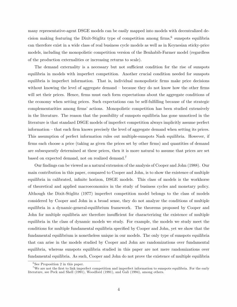
The impulse responses of the sticky-price model to a sunspots shock are reported in Figure 3.
It shows that sunspots have similar e¤ects in the sticky-price model compared to the real model
in the impact period: output, consumption, investment, and employment all increase in the initial
period. But sunspots have dramatically di¤erent e¤ects in the sticky-price model in the following
periods. In particular, consumption drops rapidly in the second period after the shock and is hence
less smooth in the sticky price model. The intuition is that when an unanticipated sunspots shock
is realized, marginal cost increases due to a self-ful�lling expected increase in aggregate demand.
Since prices are set in advance before the sunspots shocks and the sunspots are not anticipated, the
�rst period response of the model is similar to that of a real model. After the realization of sunspots,
though, prices must drop in order to maintain a high level of real balances that matches the level
of consumption. This is not possible due to sticky prices and a �xed money supply, thus forcing
consumption demand to decrease sharply. This leads �rms to reduce production and demand for
capital. Table 2 reports standard business-cycle statistics of the sticky-price model. It shows that
the markup, ��, is counter-cyclical and in�ation is procyclical. These predictions are qualitativelyconsistent with the empirical evidence.
24
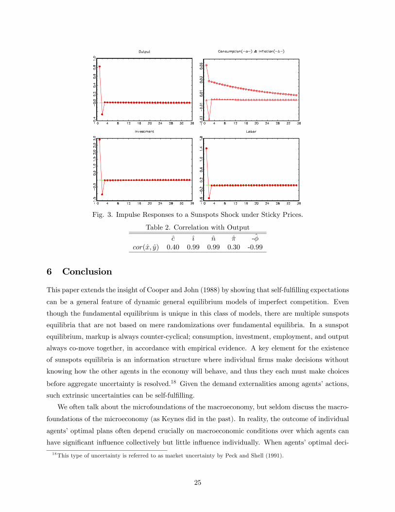
Fig. 3. Impulse Responses to a Sunspots Shock under Sticky Prices.
Table 2. Correlation with Output
c { n � -�cor(x; y) 0:40 0:99 0:99 0:30 -0:99
6 Conclusion
This paper extends the insight of Cooper and John (1988) by showing that self-ful�lling expectations
can be a general feature of dynamic general equilibrium models of imperfect competition. Even
though the fundamental equilibrium is unique in this class of models, there are multiple sunspots
equilibria that are not based on mere randomizations over fundamental equilibria. In a sunspot
equilibrium, markup is always counter-cyclical; consumption, investment, employment, and output
always co-move together, in accordance with empirical evidence. A key element for the existence
of sunspots equilibria is an information structure where individual �rms make decisions without
knowing how the other agents in the economy will behave, and thus they each must make choices
before aggregate uncertainty is resolved.18 Given the demand externalities among agents�actions,
such extrinsic uncertainties can be self-ful�lling.
We often talk about the microfoundations of the macroeconomy, but seldom discuss the macro-
foundations of the microeconomy (as Keynes did in the past). In reality, the outcome of individual
agents�optimal plans often depend crucially on macroeconomic conditions over which agents can
have signi�cant in�uence collectively but little in�uence individually. When agents�optimal deci-
18This type of uncertainty is referred to as market uncertainty by Peck and Shell (1991).
25
sions must be conditioned on their expectations of such macroeconomic conditions, such expecta-
tions can be self-ful�lling when synchronized. We show that �uctuations driven by self-ful�lling
expectations look very similar to those driven by technology shocks. Given that such �uctuations
are welfare reducing (as shown in this paper), interventionary policies are called for. The design
of optimal �scal and monetary policies to counter sunspots-driven �uctuations is a promising topic
which can be pursued in future research using the framework provided in this paper. This is par-
ticularly relevant to the fast growing New Keynesian literature of monetary policy analysis. This
literature shows that cost-push shocks to �rms�marginal cost can generate a painful in�ation-
output trade-o¤ that complicates the design of optimal monetary policies (see, e.g., Clarida, Gali,
and Gertler, 1999; Woodford, 2001; and Gali, 2002). We show in this paper that sunspots and
self-ful�lling expectations are a natural source of cost-push shocks under imperfect competition.
Appendix 1: Proof of Proposition 2
The equilibrium paths of the marginal cost in the imperfect competition model, f�tg1t=0, are
determined by the price setting behavior of the monopolistic �rms given in Equation (12). Given
a path of �, Equations (13)-(18) (plus the transversality condition) fully determine the equilibrium
allocation of the imperfect competition model. Since the utility functions and production functions
are concave, a competitive model can achieve the same equilibrium allocation if and only if it has
the same set of �rst-order conditions (but not necessarily the same production functions) as those
in the imperfect competition model.
Let the utility functions be the same in both models. Let the production function of intermediate
goods in the Dixit-Stiglitz model be denoted by y = g(k; n). Hence Equations (13) and (14) can
be expressed as w = �gn = ��nyn and r = �gk = ��r
yk ; where fw; rg denote the real wage and real
rental rate, f�n; �kg denote output elasticities of labor and capital, and � denotes the marginal cost.Consider a competitive RBC model featuring a representative �rm with the aggregate production
technology, y = f(k; n): Pro�t maximization by the representative �rm gives w = (1 � �)fn =
(1 � �)"n yn and r = (1 � �)fk = (1 � �)"n yk ; where � 2 [0; 1] denotes the income tax rate, and
f"n; "kg denote the output elasticities of labor and capital in this model. We assume that thegovernment can use lump-sum transfers to redistribute the revenue from the income tax (if any)
back to the household, so that the budget constraint of the household in the competitive model is
the same as that in the imperfect competitive model (Equation 18).
Given that the utility function and production functions are concave in both models, the two
models have the same set of equilibrium allocations if and only if the real wage and real interest rate
are the same in both models �namely, if and only if the following conditions hold: (1� �)"n = ��n;
26
(1��)"k = ��k; and (1��)("n+"k) = �(�n+�k): For example, if both models have constant returnsto scale technologies (i.e., "n+"k = 1 = �n+�k), then � = 1�� and f(�) = g(�) are the requirementsfor equivalence. Notice that the equivalence holds for any path of f�g. If � is constant (as in thefundamental equilibrium), it is then also possible to achieve equivalence without an income tax(
� = 0) in the competitive model. For example, let the production functions be Cobb-Douglas in
both models, and let �n+ �k = 1 and � = 0. In this case, a diminishing returns to scale production
technology in the competitive model with "n = ��n; "k = ��k; and "n+"k = � are the requirements
for equivalence.19�
Appendix 2: Proof of Proposition 3
Since sunspots give rise to allocations that di¤er across di¤erent sunspot states within any
period, the key of the proof is to show that in any given period, any state-dependent allocations
for consumption, hours worked, the capital stock, and the marginal cost are not optimal. As such,
the household prefers the certainty equilibrium to sunspots equilibria in the imperfect competition
model.
The �rst step in the proof is to transform the imperfect competition model to an equivalent,
representative-agent model with distortionary income taxation:
maxfct;nt;kt+1g
E0
1Xt=0
�tu(ct; 1� nt) (62)
subject to
ct + kt+1 � (1� �)kt � �tyt +Dt (63)
Et�1�tyt =� � 1�
Et�1yt; (64)
where yt = k�t n1��t is the aggregate production technology, �t is one minus the income tax rate, and
Dt = (1� �t)yt is a lump-sum government transfer which the agent takes as parametric. One can
easily verify that this representative-agent model of income taxation is equivalent to the imperfect
competition model by comparing the �rst-order conditions of the two models. This equivalence
implies that one minus the marginal cost (1 � �) in the imperfect competition model serves as adistortionary income tax in the representative agent model. This is intuitive because 1 � � is ameasure of the markup in the imperfect competition model.
In the absence of extrinsic uncertainty, constraint (64) implies � = ��1� . Given this, the optimal
paths for consumption, hours worked, and the capital stock are denoted by�c�t ; n
�t ; k
�t+1
1t=0, which
is the unique optimal allocation in the certainty equilibrium.19We assume that pro�ts (if any) are redistributed back to the representative household in both models.
27
Next, consider the case where the agent is given the option of having a random marginal cost
that is state dependent, �t(x); at the beginning of any period t and for that period only. We show
that the representative agent is worse o¤ in welfare by facing the state-dependent random marginal
cost. Let there be a continuum of states, x, in period t. Without loss of generality, assume that
x has a uniform distribution over [0; 1]. Starting at the beginning of period t, the representative
agent�s problem is to solve
max1Xs=0
�sZu (ct+s(x); 1� nt+s(x)) dx (65)
subject toZ[ct+s(x) + kt+s+1(x)� (1� �)kt+s(x)] dx �
Z ��t+s(x)yt+s(x) +Dt+s(x)
�dx (66)
Z ��t+s(x)yt+s(x)
�dx =
� � 1�
Zyt+s(x)dx (67)
Notice that constraint (66) is weaker than the constraint
ct+s(x) + kt+s+1(x)� (1� �)kt+s(x) � �t+s(x)yt+s(x) +Dt+s(x): (660)
The household�s income is constant (risk free) in constraint (66) while it is stochastic in constraint
(660). However, in a state-independent allocation, these two constraints are the same. Substituting
the equality in the second constraint (67) into the �rst constraint (66), the period-budget constraint
becomesZ[ct+s(x) + kt+s+1(x)� (1� �)kt+s(x)] dx �
� � 1�
Zyt+s(x)dx+
ZDt+s(x)dx: (68)
In period t, let ct =Z 1
0ct(x)dx and nt =
R 10 nt(x)dx. It is clear that the state-independent
allocation fct; ntg satis�es the budget constraint (68) in period t:
ct +
Zkt+1(x)dx� (1� �)kt � � � 1
�
Zyt(x)dx+
ZDt(x)dx (69)
� � � 1�
k�t n1��t +
ZDt(x)dx; (70)
where kt is independent of x because it is determined in the last period t � 1, and the secondinequality (70) is based on the concavity of the production function. By the concavity of the utility
function, we have
28
Zu(ct(x); 1� nt(x))dx � u(ct; 1� nt): (71)
Hence, the state-independent allocation fct; ntg gives higher welfare by increasing the agent�s utilityand output in period t. As such, there are no state-dependent allocations for consumption and hours
worked in period t that can yield higher welfare than the allocation fct; ntg. Since the optimal hours
worked, nt; is state-independent, it follows that yt(x) = k�t n1��t is also state-independent in period
t. Hence Dt(x) = 1�yt(x) is also state-independent.
In the next period, the concavity of the production function f(k; n) implies that a state-
independent allocation, fkt+1; nt+1g =�Rkt+1(x)dx;
Rnt+1(x)dx
, can yield at least as much
output as any state-dependent allocation fnt+1(x); kt+1(x)g:
f(kt+1; nt+1) �Zf(kt+1(x); nt+1(x))dx: (72)
For the same reason, we have Dt+1 �RDt+1(x)dx in equilibrium. It is also clear that the state-
independent capital stock, kt+1 =Rkt+1(x)dx, can cost no more resources in period t than the
expected capital stockRkt+1(x)dx. Hence a state-independent allocation for kt+1 is optimal and
it satis�es the budget constraints in both period t and period t+ 1 simultaneously. Therefore, the
state-independent allocation fct; nt; kt+1g is both feasible and optimal in period t. Since the utilityfunction is increasing in ct, the period-t budget constraint binds with equality under the optimal
allocation fct; nt; kt+1g:
ct + kt+1 � (1� �)kt =� � 1�
yt +Dt: (73)
The same logic applies to periods t+ 1; t+ 2; :::; and so on, ad in�nitum. Therefore, the state-
independent allocation fct+s; nt+s; kt+s+1g1s=0 is better than any random allocation. Under the
state-independent allocation, the resource constraints (73) for all t are the same as the resource
constraints speci�ed in (63) (which hold with equality when � = ��1� ). Hence, the state-independent
allocation is also equivalent to the allocation�c�t ; n
�t ; k
�t�11t=0
under the certainty equilibrium.�
Appendix 3: Solving the Sticky-Price Model
Using circum�ex variables to denote deviations in log, x = log(xt=�x), the log-linearized �rst-
order conditions of the sticky-price model are summarized below:
(�+ )nt = �t + �kt � ct (74)
29
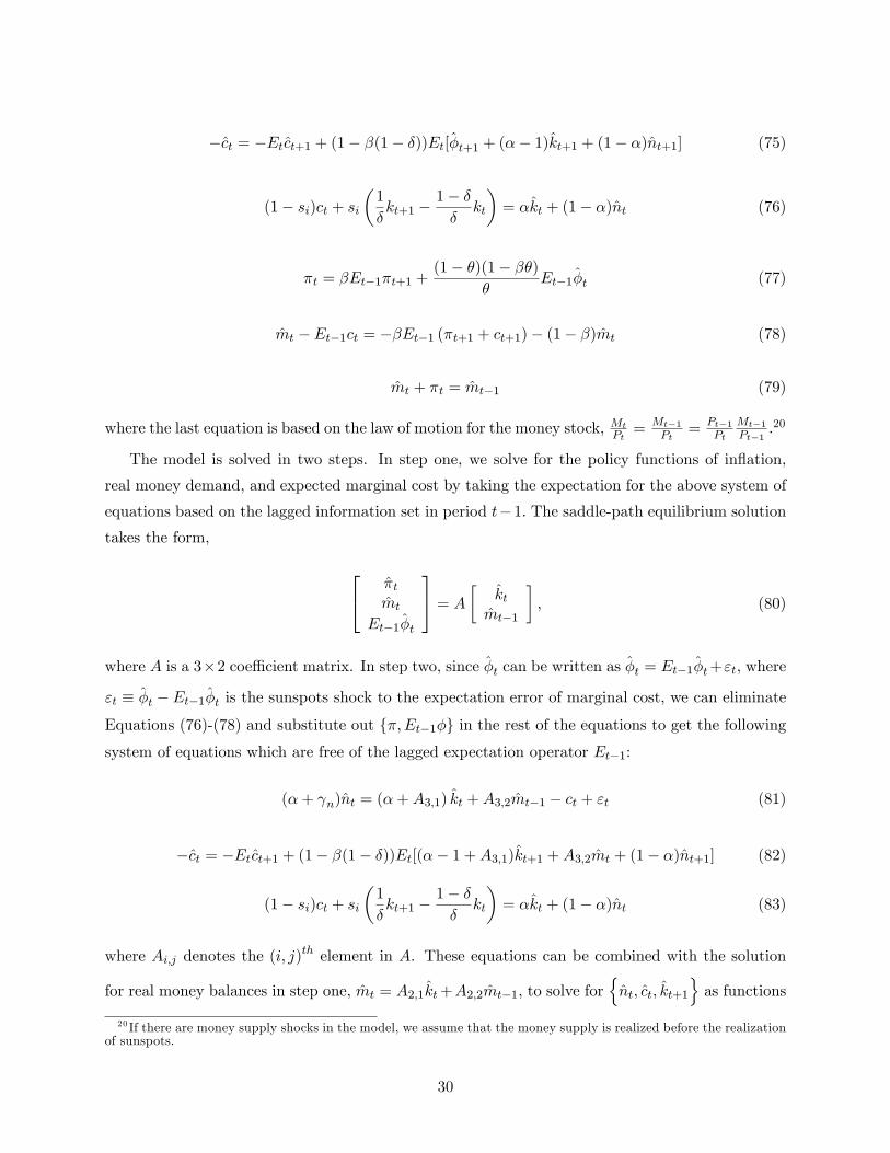
�ct = �Etct+1 + (1� �(1� �))Et[�t+1 + (�� 1)kt+1 + (1� �)nt+1] (75)
(1� si)ct + si�1
�kt+1 �
1� ��kt
�= �kt + (1� �)nt (76)
�t = �Et�1�t+1 +(1� �)(1� ��)
�Et�1�t (77)
mt � Et�1ct = ��Et�1 (�t+1 + ct+1)� (1� �)mt (78)
mt + �t = mt�1 (79)
where the last equation is based on the law of motion for the money stock, MtPt= Mt�1
Pt= Pt�1
Pt
Mt�1Pt�1
.20
The model is solved in two steps. In step one, we solve for the policy functions of in�ation,
real money demand, and expected marginal cost by taking the expectation for the above system of
equations based on the lagged information set in period t�1: The saddle-path equilibrium solutiontakes the form,
24 �tmt
Et�1�t
35 = A � ktmt�1
�; (80)
where A is a 3�2 coe¢ cient matrix. In step two, since �t can be written as �t = Et�1�t+"t, where
"t � �t � Et�1�t is the sunspots shock to the expectation error of marginal cost, we can eliminateEquations (76)-(78) and substitute out f�;Et�1�g in the rest of the equations to get the followingsystem of equations which are free of the lagged expectation operator Et�1:
(�+ n)nt = (�+A3;1) kt +A3;2mt�1 � ct + "t (81)
�ct = �Etct+1 + (1� �(1� �))Et[(�� 1 +A3;1)kt+1 +A3;2mt + (1� �)nt+1] (82)
(1� si)ct + si�1
�kt+1 �
1� ��kt
�= �kt + (1� �)nt (83)
where Ai;j denotes the (i; j)th element in A. These equations can be combined with the solution
for real money balances in step one, mt = A2;1kt+A2;2mt�1, to solve fornnt; ct; kt+1
oas functions
20 If there are money supply shocks in the model, we assume that the money supply is realized before the realizationof sunspots.
30
of the states,nkt; mt�1; "t
o. The fact that there is a unique fundamental equilibrium in this class
of models implies that there are just enough explosive eigenvalues as control variables to solve for
the saddle-path decision rules.
31
References
[1] Alvarez, F. and R. E. Lucas, Jr., 2004, General equilibrium analysis of the Eaton-Kortum
model of international trade, Working Paper, University of Chicago.
[2] Azariadis, C., 1981, Self-ful�lling prophecies, Journal of Economic Theory 25(3), 380-396.
[3] Benhabib, J. and R. Farmer, 1994, Indeterminacy and increasing returns, Journal of Economic
Theory 63(1), 19-41.
[4] Benhabib, J. and R. Farmer, 1996, Indeterminacy and sector-speci�c externalities, Journal of
Monetary Economics 37(3), 421-443.
[5] Benhabib, J. and R. Farmer, 1999, Indeterminacy and sunspots in macroeconomics, Handbook
of Macroeconomics, eds. John Taylor and Michael Woodford, North-Holland, New York, vol.
1A, 387-448.
[6] Bils, M., 1987, The cyclical behavior of marginal cost and price, American Economic Review
77(5), 838-855.
[7] Blanchard, O. and N. Kiyotaki, 1987, Monopolistic competition and the e¤ects of aggregate
demand, American Economic Review 77(4), 647-666.
[8] Blanchard, O. and C. Kahn, 1980, The solution of linear di¤erence models under rational
expectations, Econometrica 48(5), 1305-1312.
[9] Calvo, G., 1983, Staggered prices in a utility-maximizing framework, Journal of Monetary
Economics 12 (3), 383-398.
[10] Cass, D. and K. Shell, 1983, Do sunspots matter? Journal of Political Economy 91(2), 193-227.
[11] Clarida, R., J. Gali, and M. Gertler, 1999, The science of monetary policy: A New Keynesian
perspective, Journal of Economic Literature 37 (4), 1661-1707.
[12] Clarida, R., J. Gali, and M. Gertler, 2001, Optimal Monetary Policy in Open versus Closed
Economies: An Integrated Approach, The American Economic Review.
[13] Cooper, R. and A. John, 1988, Coordinating coordination failures in Keynesian models, The
Quarterly Journal of Economics 103(3), 441-463.
[14] Dixit, A. and J. Stiglitz, 1977, Monopolistic competition and optimum product diversity,
American Economic Review 67(3), 297-308.
32
[15] Farmer, R., 1999, Macroeconomics of Self-ful�lling Prophecies, Second Edition, Cambridge,
MA: The MIT Press.
[16] Farmer, R. and Guo, J., 1994, Real business cycles and the animal spirits hypothesis, Journal
of Economic Theory 63(1), 42-72.
[17] Gali, J., 1994, Monopolistic competition, business cycles, and the composition of aggregate
demand, Journal of Economic Theory 63(1), 73-96.
[18] Gali, J., 2002, New perspectives on monetary policy, in�ation, and the business cycle, NBER
Working Paper 8767.
[19] Georges, C., 1995, Adjustment costs and indeterminacy in perfect foresight models, Journal
of Economic Dynamics and Control 19(1-2), 39-50.
[20] Kiyotaki, N., 1988, Multiple expectational equilibria under monopolistic competition, The
Quarterly Journal of Economics 103(4), 695-713.
[21] Kydland, F. and E. Prescott, 1982, Time to build and aggregate �uctuations, Econometrica
50(6), 1345-70.
[22] Lane, P.R., M.B. Devereux, and J. Xu, 2005, Cost-Push Shocks and Monetary Policy in Open
Economics, Working Paper, University of British Columbia.
[23] Mankiw, N.G. and R. Reis, 2002, Sticky information versus sticky prices: A proposal to replace
the New Keynesian Phillips Curve, The Quarterly Journal of Economics 117(4), 1295-1328.
[24] Martins, J., S. Scapetta, and D. Pilat, 1996, Mark-up pricing, market structure and the
business cycle, OECD Economic Studies 27, 71-105.
[25] Peck, J. and K. Shell, 1991, Market uncertainty: Correlated and sunspot equilibria in imper-
fectly competitive economies, The Review of Economic Studies 58(5), 1011-1029.
[26] Ravenna, F. and C. Walsh, 2004, Optimal Monetary Policy with the Cost Channel, Journal
of Monetary Economics, forthcoming.
[27] Rotemberg, J. and M. Woodford, 1991, Markups and the business cycle, in O.J. Blanchard and
S. Fischer (eds.), NBER Macroeconomic Annual 1991, Cambridge, MA: MIT Press, 63-129.
[28] Rotemberg, J. and M. Woodford, 1999, Markups and the business cycle, in Taylor, J.B. and
M. Woodford (eds.), Handbook of Macroeconomics, Vol. 1(B), Amsterdam: North-Holland.
33
[29] Shell, K., 1977, Monnaie et allocation intertemporelle, Mimeo, Séminaire Roy-Malinvaud,
Centre National de la Recherche Scienti�que, Paris, November.
[30] Steinsson, J., 2003, Optimal monetary policy in an economy with in�ation persistence, Working
Paper, Harvard University.
[31] Walsh, C., 1999, Monetary Policy Trade-O¤s in the Open Economy, Working Paper, University
of California, Santa Cruz.
[32] Wen, Y., 1998a, Capacity utilization under increasing returns to scale, Journal of Economic
Theory 81(1), 7-36.
[33] Wen, Y., 1998b, Indeterminacy, dynamic adjustment costs, and cycles, Economics Letters
59(1), 213-216.
[34] Woodford, M., 1986, Stationary sunspot equilibria in a �nance constrained economy, Journal
of Economic Theory 40(1), 128-137.
[35] Woodford, M., 1991, Self-ful�lling expectations and �uctuations in aggregate demand. In:
N.G. Mankiw and D. Romer (eds.), New Keynesian Economics: Coordination Failures and
Real Rigidities, Vol. 2, Cambridge, MA: MIT Press, 77-110.
[36] Woodford, M., 2001, In�ation stabilization and welfare, NBER Working Paper 8071.
[37] Yun, T., 1996, Nominal price rigidity, money supply endogeneity, and business cycles, Journal
of Monetary Economics 37(2), 345�370.
34