Impes Examples

TPG4160 Reservoir Simulation 2015 Hand-out note 7

Norwegian University of Science and Technology Professor Jon Kleppe Department of Petroleum Engineering and Applied Geophysics 26/1/15

page 1 of 11

SATURATED OIL-GAS SIMULATION - IMPES SOLUTION The major difference between two-phase oil-water flow and two-phase, saturated oil-gas flow is that the solution gas terms have to be included in the flow equations. Recall from the previous review of Black Oil PVT behavior that the oil density at reservoir conditions is defined as:

ρo =ρoS + ρgSRso

Bo

First of all, for a saturated oil-gas system, the oil pressure is per definition equal to the bubble point pressure, or saturation pressure: Po = Pbp and, in addition, So ≥ 0. The implication of these definitions, is that the formation volume factor and the solution gas-oil ratio are functions of oil pressure only,

Bo = f (Po )

Rso = f (Po )

Thus, for saturated oil, the solution gas term is no longer constant and will not be canceled out of the oil equation, as it did in single phase flow and in oil-water flow. We will, for mass balance purposes, separate the oil density into two parts, one that remains liquid at the surface and one that becomes gas:

ρo =ρoS + ρgSRso

Bo=ρoSBo

+ρgSRsoBo

= ρoL + ρoG

We will write the oil mass balance so that its continuity equation includes the liquid part only, while the gas mass balance includes both free gas and solution gas in the reservoir, and thus all free gas at the surface:

−∂∂x

ρoLuo( ) = ∂∂t

φρoLSo( )

−∂∂x

ρgug +ρoGuo( ) = ∂∂t

φ ρgSg +ρoGSo( )[ ] .

In the gas equation, the solution gas will of course flow with the rest of the oil in the reservoir, at oil relative permeability, viscosity and pressure. The Darcy equations for the two phases are:

uo = −kkroµo

∂Po∂x

ug = −kkrgµg

∂Pg∂x

.

Substituting Darcy's equations and the liquid oil density and the solution gas density definitions, together with the standard free gas density definition,



page 2 of 11

ρg =ρgSBg

into the continuity equations, and including production/injection terms in the equations, results in the following flow equations for the two phases:

∂∂x

kkroµo Bo

∂Po∂x

⎛

⎝ ⎜

⎞

⎠ ⎟ − ′ q o =

∂∂t

φSoBo

⎛

⎝ ⎜

⎞

⎠ ⎟

and

∂∂x

kkrg

µ gBg

∂Pg

∂x+ Rso

kkroµoBo

∂Po∂x

⎛

⎝ ⎜

⎞

⎠ ⎟ − ′ q g − Rso ′ q o =

∂∂t

φSg

Bg+ Rso

φSoBo

⎛

⎝ ⎜

⎞

⎠ ⎟ ,

where

Pcog = Pg − Po So + Sg = 1 .

Relative permeabilities and capillary pressure are functions of gas saturation, while formation volume factors, viscosities and porosity are functions of pressures. Fluid properties are defined by the standard Black Oil model for saturated oil, as we have reviewed previously. Before proceeding, we shall also review the relative permeabilities and capillary pressure relationships for oil-gas systems. Review of oil-gas relative permeabilities and capillary pressure Normally, only drainage curves are required in gas-oil systems, since gas displaces oil. However, sometimes reimbibition of oil into areas previously drained by gas displacement may happen. Reimbibition phenomena may be particularly important in gravity drainage processes in fractured reservoirs. Starting with the porous rock completely filled with oil, and displacing by gas, the drainage relative permeability and capillary pressure curves will be defined:

If the process is reversed when all mobile oil has been displaced, by injecting oil to displace the gas, imbibition curves are defined as:

So1.0

Kr

SoSorg 1-Sgc

gasoilSo=1

Drainageprocess

Sorg

Pdog

Pcog



page 3 of 11

The shape of the gas-oil curves will of course depend on the surface tension properties of the system, as well as on the rock characteristics. Discretization of flow equations The discretization procedure for oil-gas equations is very much similar to the one for oil-water equations. In fact, for the oil equation, it is identical, with a small exception for the saturation, which now is for gas and not water. Thus, the discretized oil equation may be written:

Txoi +1 2 Poi+1 − Poi( ) + Txoi−1 2 Poi−1 − Poi( ) − ′ q oi

= Cpooi Poi − Poit( ) + Csgoi Sgi − Sgi

t( ), i = 1,N

Definitions of the terms in the equation are given below:

Txoi+1 2 =2λoi+1 2

ΔxiΔxi+1ki+1

+Δxiki

⎛

⎝ ⎜

⎞

⎠ ⎟

Txoi−1 2 =2λoi−1 2

ΔxiΔxi−1ki−1

+Δxiki

⎛

⎝ ⎜

⎞

⎠ ⎟

where

λo =kroµoBo

and the upstream mobilities are selected as:

λoi+1/ 2 =λoi+1 if Poi+1 ≥ Poiλoi if Poi+1 < Poi

⎧ ⎨ ⎩

λoi−1/ 2 =λoi−1 if Poi−1 ≥ Poiλoi if Poi−1 < Poi

⎧ ⎨ ⎩

The right side coefficients are:

Cpooi =φi (1− Sgi )

ΔtcrBo

+d (1/ Bo )dPo

⎡

⎣ ⎢

⎤

⎦ ⎥ i

Csgoi = −φ i

BoiΔti

oil

So

Kr

SoSorg 1-Sgro

oilgasSo=Sor

Imbibitionprocess

Sorg

Pcog

1-Sgro

oil gas



page 4 of 11

Left hand side of gas equation For the gas equation, we will partly use similar approximations as for the oil equation, and also introduce new approximations for the solution gas terms. First,

∂∂x

kkrgµ gBg

∂Pg∂x

+ Rsokkro

µoBo

∂Po∂x

⎛

⎝ ⎜

⎞

⎠ ⎟ =

∂∂x

kkrgµg Bg

∂Pg∂x

⎛

⎝ ⎜

⎞

⎠ ⎟ +

∂∂x

Rsokkro

µoBo

∂Po∂x

⎛

⎝ ⎜

⎞

⎠ ⎟

Then, we use similar approximations for the free gas term as we did for oil and for water:

∂∂x

kkrgµg Bg

∂Pg∂x

⎛

⎝ ⎜

⎞

⎠ ⎟ i

≈ Txgi+1 / 2 (Pgi+1 − Pgi ) + Txgi−1/ 2 (Pgi−1 − Pgi )

where the gas transmissibilities are defined as:

Txgi+1 2 =2λgi+1 2

ΔxiΔxi+1ki+1

+Δxiki

⎛

⎝ ⎜

⎞

⎠ ⎟

Txgi−1 2 =2λgi−1 2

ΔxiΔxi−1ki−1

+Δxiki

⎛

⎝ ⎜

⎞

⎠ ⎟

where

λg =krgµg Bg

and the upstream mobilities are selected as:

λgi+1/ 2 =λgi+1 if Pgi+1 ≥ Pgiλgi if Pgi+1 < Pgi

⎧ ⎨ ⎩

λgi−1/ 2 =λgi−1 if Pgi−1 ≥ Pgiλgi if Pgi−1 < Pgi

⎧ ⎨ ⎩

The solution gas term may be approximated as the oil flow term, with the exception that the solution term has to be included as follows:

∂∂x

Rsokkro

µo Bo

∂Po∂x

⎛

⎝ ⎜

⎞

⎠ ⎟ i

≈ RsoTxo( )i+1 / 2 (Poi+1 − Poi ) + RsoTxo( )i−1/ 2(Poi−1 − Poi )

For the solution gas-oil ratios, we will again use the upstream principle, just as for the mobilities:

Rsoi+1/ 2 =Rsoi+1 if Poi+1 ≥ PoiRsoi if Poi+1 < Poi

⎧ ⎨ ⎩

Rsoi−1/ 2 =Rsoi−1 if Poi−1 ≥ PoiRsoi if Poi−1 < Poi

⎧ ⎨ ⎩



page 5 of 11

Right hand side of gas equation The right hand side of the gas equation consists of a free gas term and a solution gas term:

∂∂t

φSgBg

+φRsoSoBo

⎛

⎝ ⎜

⎞

⎠ ⎟ =

∂∂t

φSgBg

⎛

⎝ ⎜

⎞

⎠ ⎟ +

∂∂t

φRsoSoBo

⎛

⎝ ⎜

⎞

⎠ ⎟

Using similar approximations as for water for the free gas term, we may write:

∂∂t

φSgBg

⎛

⎝ ⎜

⎞

⎠ ⎟ ≈

φ i SgiΔt

crBg

+d (1/ Bg )dPg

⎛

⎝ ⎜

⎞

⎠ ⎟ i

(Poi − Poit ) +

dPcogdSg

⎛

⎝ ⎜

⎞

⎠ ⎟ i

(Sgi − Sgit )

⎡

⎣ ⎢ ⎢

⎤

⎦ ⎥ ⎥

+φ iBgiΔt

(Sgi − Sgit ) .

The solution gas term may be expanded into:

∂∂t

φRsoSoBo

⎛

⎝ ⎜

⎞

⎠ ⎟ = Rso

∂∂t

φSoBo

⎛

⎝ ⎜

⎞

⎠ ⎟ +

φSoBo

∂Rso∂t

The first term is identical to the right hand side of the oil equation, multiplied by Rso. Thus,

Rso∂∂t

φSoBo

⎛

⎝ ⎜

⎞

⎠ ⎟

⎡

⎣ ⎢

⎤

⎦ ⎥ i

≈ RsoiCpooi + RsoiCsgoi

For the second term, the following approximation may be used:

φSoBo

∂Rso∂t

⎛

⎝ ⎜

⎞

⎠ ⎟ i

=φSoBo

dRsodPo

∂Po∂t

⎛

⎝ ⎜

⎞

⎠ ⎟ i

≈1Δt

φSoBo

dRsodPo

⎛

⎝ ⎜

⎞

⎠ ⎟ i

Poi − Poit( )

Then, combining the terms, the approximation of the gas equation becomes:

Txgi +1 2 Poi+1 − Poi( ) + Pcogi +1 − Pcogi( )[ ] + Txgi−1 2 Poi−1 − Poi( ) + Pcogi−1 − Pcogi( )[ ] − ′ q gi

+ RsoTxo( )i +1 2 Poi+1 − Poi( ) + RsoTxo( )i−1 2 Poi−1 − Poi( ) − Rso ′ q o( ) i

= Cpogi Poi − Poit( ) + Csggi Sgi − Sgi

t( ), i = 1,N

where

Cpogi =φ iΔ t

SgcrBg

+d(1/ Bg )dPg

⎛

⎝ ⎜

⎞

⎠ ⎟ + Rso (1 − Sg )

crBo

+d(1/ Bo)dPo

⎛

⎝ ⎜

⎞

⎠ ⎟ +

(1− Sg)Bo

dRsodPo

⎡

⎣ ⎢ ⎢

⎤

⎦ ⎥ ⎥ i

and

Csggi =φiΔt

SgcrBg

+d(1/ Bg )dPg

⎛

⎝ ⎜

⎞

⎠ ⎟ dPcogdSg

−RsoBo

+1Bg

⎡

⎣ ⎢ ⎢

⎤

⎦ ⎥ ⎥ i

The derivative terms appearing in the expressions above:

d (1/ Bo )dPo

⎛

⎝ ⎜

⎞

⎠ ⎟ i

,d (1/ Bg )dPg

⎛

⎝ ⎜

⎞

⎠ ⎟ i

,dRsodPo

⎛

⎝ ⎜

⎞

⎠ ⎟ i

anddPcogdSg

⎛

⎝ ⎜

⎞

⎠ ⎟ i

are all computed numerically for each time step based on the input table to the model.



page 6 of 11



page 7 of 11

Boundary conditions The boundary conditions for oil-gas systems are similar to those of oil-water systems. Normally, we inject gas in a grid block at constant surface rate or at constant bottom hole pressure, and produce oil and gas from a grid block at constant bottom hole pressure, or at constant surface oil rate. As for oil-water flow, we may sometimes want to specify constant reservoir voidage rate, where either the rate of injection of gas is to match a specified rate of oil and gas production at reservoir conditions, so that average reservoir pressure remains constant, or the reservoir production rate is to match a specified gas injection rate. Constant gas injection rate Again, as for water injection, a gas rate term is already included in the gas equation. Thus, for a constant surface gas injection rate of Qgi (negative) in a well in grid block i : ′ q gi = Qgi /(AΔxi ) . Then, at the end of a time step, after having solved the equations, the bottom hole injection pressure for the well may be calculated using the well equation: )( ibhiggiigi PPWCQ −= λ . The well constant in the equation above is defined just as for oil-water flow:

WCi =2πkih

ln( rerw)

,

where rw is the well radius and the drainage radius is theoretically defined as:

re =ΔyΔxiπ

.

As for water injection, we will use the sum of the mobilities of the fluids present in the injection block in the well equation. Thus, the following well equation is used for the injection of gas in an oil-gas system:

QgiBgi = WCikroiµoi

+krgiµ gi

⎛

⎝ ⎜

⎞

⎠ ⎟ (Pgi − Pbhi ),

or

Qgi = WCiBoiBgi

λoi +λgi⎛

⎝ ⎜

⎞

⎠ ⎟ (Pgi − Pbhi )

If the injection wells are constrained by a maximum bottom hole pressure, to avoid fracturing of the formation, this should be checked at the end of each time step, and, if necessary, be followed by a reduction of the injection rate, or by conversion of the well to a constant bottom hole pressure injection well. Just as for the water injection case, capillary pressure is normally neglected in the well equation, particularly in the case of field scale simulation, so that the well equation becomes:

Qgi = WCiBoiBgi

λoi +λgi⎛

⎝ ⎜

⎞

⎠ ⎟ (Poi − Pbhi ) .

For gas-oil flow, the capillary pressure is normally small, so that even in simulation of cores used in laboratory experiments, the errors resulting from neglecting capillary pressure in the well equation will be small.



page 8 of 11

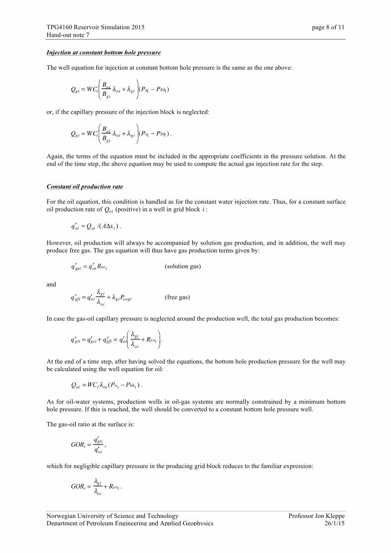
Injection at constant bottom hole pressure The well equation for injection at constant bottom hole pressure is the same as the one above:

Qgi = WCiBoiBgi

λoi +λgi⎛

⎝ ⎜

⎞

⎠ ⎟ (Pgi − Pbhi )

or, if the capillary pressure of the injection block is neglected:

Qgi = WCiBoiBgi

λoi +λgi⎛

⎝ ⎜

⎞

⎠ ⎟ (Poi − Pbhi ) .

Again, the terms of the equation must be included in the appropriate coefficients in the pressure solution. At the end of the time step, the above equation may be used to compute the actual gas injection rate for the step. Constant oil production rate For the oil equation, this condition is handled as for the constant water injection rate. Thus, for a constant surface oil production rate of Qoi (positive) in a well in grid block i : )/( ioioi xAQq Δ=′ . However, oil production will always be accompanied by solution gas production, and in addition, the well may produce free gas. The gas equation will thus have gas production terms given by:

isooigsi Rqq ′=′ (solution gas)

and

′ q gfi = ′ q oiλgi

λoi+λgiPcogi (free gas)

In case the gas-oil capillary pressure is neglected around the production well, the total gas production becomes:

′ q gti = ′ q gsi + ′ q gfi = ′ q oiλgi

λoi+ Rsoi

⎛

⎝ ⎜

⎞

⎠ ⎟ .

At the end of a time step, after having solved the equations, the bottom hole production pressure for the well may be calculated using the well equation for oil: )( ibhiooiioi PPWCQ −= λ . As for oil-water systems, production wells in oil-gas systems are normally constrained by a minimum bottom hole pressure. If this is reached, the well should be converted to a constant bottom hole pressure well. The gas-oil ratio at the surface is:

GORi =

′ q gti

′ q oi,

which for negligible capillary pressure in the producing grid block reduces to the familiar expression:

GORi =

λgiλoi

+ Rsoi .



page 9 of 11

Frequently, well rates are constrained by maximum GOR levels, due to limitations in process equipment. If a maximum gas-oil ratio level is exceeded for a well, the highest GOR grid block may be shut in, in case more than one gridblocks are perforated, or the production rate may have to be reduced. Production at constant reservoir voidage rate As for the oil-water system, the total production of fluids from a well in block i , at reservoir conditions, is to match the reservoir injection volume so that the reservoir pressure remains approximately constant. Thus, injginjggigioioi BQBQBQ −=+ , which, again assuming that capillary pressure is negligible, leads to:

′ q oi =λoi

λoiBoi + λgiBgi(−QgiBginj) /(AΔxi )

and

′ q gi =λgi

λoiBoi + λgiBgi(−QgiBginj ) /(AΔxi ) .

The solution gas rate term thus becomes:

Rsoi ′ q oi =Rsoiλoi

λoiBoi + λgiBgi(−QgiBginj ) /(AΔxi )

Production at constant bottom hole pressure Using a production well in grid block i with constant bottom hole pressure, Pbhi , as an example, we have an oil rate of:

Qgi = WCiλoi(Poi − Pbhi ) and a free gas rate of: Qgi = WCiλgi(Pgi − Pbhi ) . Substituting into the flow terms in the flow equations, the oil rate becomes:

′ q oi =WCiAΔxi

λoi(Poi − Pbhi ) ,

and the free gas rate:

′ q gi =WCiAΔxi

λgi(Pgi − Pbhi )

and finally the solution gas rate:

Rsoi ′ q oi = RsoiWCiAΔxi

λoi(Poi − Pbhi )

Again, the flow rate terms have to be included in the appropriate matrix coefficients when solving for pressures. At the end of each time step, actual rates are computed by the equations above, and GOR is computed as in the previous cases.



page 10 of 11



page 11 of 11

Solution by IMPES method The procedure for IMPES solution is similar to the oil-water case. Thus, we make the same assumptions in regard to the coefficients:

tcog

tsgg

tsgo

tpog

tpoo

txg

txo

P

CC

CC

TT

,

,

,

.

Having made these approximations, the discretized flow equations become:

Txoi +1/ 2t Poi +1 − Poi( ) + Txoi−1/ 2

t Poi−1 − Poi( ) − ′ q oi

= Cpooit Poi − Poi

t( ) + Csgoit Sgi − Sgi

t( ), i = 1,N

Txgi +1/ 2

t Poi +1 − Poi( ) + Pcogi+1 − Pcogi( ) t[ ]+Txgi−1 / 2

t Poi−1 − Poi( ) + Pcogi−1 − Pcogi( ) t[ ] − ′ q gi

+ RsoTxo( )i +1/ 2t Poi +1 − Poi( ) + RsoTxo( ) i−1 / 2

t Poi−1 − Poi( ) − Rso ′ q o( ) i

= Cpogit Poi − Poi

t( ) + Csggit Sgi − Sgi

t( ), i = 1,N

IMPES pressure solution The pressure equation for the saturated oil-gas becomes:

Txoi+1 / 2t +α i Txgi +1/ 2

t + RsoTxo( ) i+1 / 2t[ ]{ } Poi +1 − Poi( ) +

Txoi−1 / 2t +α i Txgi−1/ 2

t + RsoTxo( ) i−1 / 2t[ ]{ } Poi−1 − Poi( )

+α iTxgi+1 / 2t Pcogi +1 − Pcogi( ) t +α iTxgi−1/ 2

t Pcogi−1 − Pcogi( )t

− ′ q oi −α i ′ q g + Rsot ′ q oi( ) i

=

Cpooit +α iCpogi

t( ) Poi − Poit( ), i = 1, N

where α i = −Csgoi

t /Csggit .

The pressure equation may now be rewritten as:

NidPcPbPa iioiioiioi ,1,11 ==++ +−

where

ai = Txoi−1/ 2t +α i Tsg+ RsoTxo( )i−1/ 2

t ci = Txoi+1 / 2

t +α i Tsg+ RsoTxo( ) i+1 / 2t

bi = −Txoi−1/ 2

t − Txoi+1 / 2t −Cpooi

t −α i Txg+ RsoTxo( ) i−1/ 2t + Txg + RsoTxo( )i+1 / 2

t +Cpogit[ ]



page 12 of 11

di = −(Cpooi

t +α iCpogit )Poi

t + ′ q oi +α i ′ q g + Rso ′ q o( ) i

−α iTxgi +1/ 2t (Pcogi+1 − Pcogi )

t −α iTxgi−1/ 2t (Pcogi−1 − Pcogi )

t

Modifications for boundary conditions Again, all rate specified well conditions are included in the rate terms ′ q oi , ′ q gi and Rsoi ′ q oi . With the coefficients involved at old time level, coefficients, these rate terms are already appropriately included in the di term above. For injection of gas at bottom hole pressure specified well conditions, the following expression applies (again using the case of neglected capillary pressure as example; however, capillary pressure can easily be included):

Qgi = WCiBoiBgi

λoi +λgi⎛

⎝ ⎜

⎞

⎠ ⎟ t

(Poi − Pbhi ).

In a block with a well of this type, the following matrix coefficients are modified (assuming that there is not a production well in the injection block):

bi = −Txoi−1/ 2t − Txoi+1 / 2

t −Cpooit

−α iWCiAΔxi

BoiBgi

λoi +λgi⎛

⎝ ⎜

⎞

⎠ ⎟ t

+ Txg + RsoTxo( )i−1/ 2t + Txg+ RsoTxo( ) i+1 / 2

t +Cpogit

⎡

⎣ ⎢ ⎢

⎤

⎦ ⎥ ⎥

di = −(Cpooi

t +α iCpogit )Poi

t −α iWCiΔxi

BoiBgi

λoi + λgi⎛

⎝ ⎜

⎞

⎠ ⎟ t

Pbhi

−α iTxgi+1/ 2t (Pcogi+1 − Pcogi )

t −α iTxgi−1/ 2t (Pcogi−1 − Pcogi )

t

For production at bottom hole pressure specified well conditions, we have the following expressions:

′ q oi =WCiAΔxi


′ q gi =WCiAΔxi

λgi(Pgi − Pbhi )

and

Rsoi ′ q oi =WCiAΔxi

Rsoiλoi(Poi − Pbhi ) .

In a block with a well of this type, the following matrix coefficients are modified:

bi = −Txoi−1/ 2t − Txoi+1 / 2

t −Cpooit −

WCiAΔxi

λoit

−α iWCiAΔxi

Rsoiλoi +λgi( )t + Txg + RsoTxo( )i−1/ 2t + Txg + RsoTxo( )i+1/ 2

t + Cpogit⎡

⎣ ⎢ ⎤ ⎦ ⎥

di = −(Cpooit +α iCpogi

t )Poit − WCi

Δxiλoi

t Pbhi −α iWCi

Δxiλgi + Rso ′ q o( ) i

tPbhi

−α iTxgi +1/ 2t (Pcogi+1 − Pcogi )

t +α iTxgi−1/ 2t (Pcogi−1 − Pcogi )

t

As for oil-water, the pressure equation may now be solved for oil pressures by using Gaussian elimination.



page 13 of 11

IMPES saturation solution Having obtained the oil pressures above, we need to solve for gas saturations using either the oil equation or the gas equation. In the following we will use the oil equation for this purpose:

Txoi +1/ 2

t Poi +1 − Poi( ) + Txoi−1/ 2t Poi−1 − Poi( ) − ′ q oi

= Cpooit Poi − Poi

t( ) + Csgoit Sgi − Sgi

t( ), i = 1,N

Again, since gas saturation only appears as an unknown in the last term on the right side of the oil equation, we may solve for it explicitly:

Sgi = Sgit +

1Csgoi

t Txoi+1 / 2t Poi +1 − Poi( ) + Txoi−1/ 2

t Poi−1 − Poi( ) − ′ q oi −Cpooit Poi − Poi

t( )[ ], i = 1,N

For grid blocks having pressure specified production wells, we make appropriate modifications, as discussed previously:

Sgi = Sgit + 1

Csgoit Txoi+1/ 2

t Poi+1 − Poi( ) +Txoi−1/ 2t Poi−1 − Poi( ) − WCi

AΔxiλoit Poi − Pbhi

t( ) − Cpooit Poi − Poit( )⎡ ⎣ ⎢

⎤ ⎦ ⎥

i = 1,N Having obtained oil pressures and water saturations for a given time step, well rates or bottom hole pressures may be computed, if needed, from, from the following expression for an injection well:

′ q gi =WCiAΔxi

BoiBgi

λoi + λgi⎛

⎝ ⎜

⎞

⎠ ⎟ (Poi − Pbhi ),

and for a production well:

′ q oi =WCiAΔxi


′ q gi =WCiAΔxi

λgi(Pgi − Pbhi )

and

Rsoi ′ q oi =WCiAΔxi

Rsoiλoi(Poi − Pbhi ) .

The surface gas-oil ratio is computed as:

GORi =

′ q gi + Rsoi ′ q oi

′ q oi.

Required adjustments in well rates and well pressures, if constrained by upper or lower limits are made at the end of each time step, before all coefficients are updated and we can proceed to the next time step. Applicability of IMPES method Applicability of the IMPES method for oil-gas systems is fairly much as for oil-water systems. However, since saturation changes in gas-oil systems generally are more rapid than for oil-water systems, due to the fact that the gas viscosity is much smaller than for liquids, smaller time step sizes may be required.

Textbook: Chapter 6, p. 57-62, Appendix B, p. 132-139, Appendix C, p. 140-144



page 14 of 11

Documents

Impes Examples