Implementation and analysis of

a multi-channel dynamic-range compressor

Johannes Käsbach s081558 Lyngby, June 26th 2009

2

Table of contents Abstract .................................................................................................................................................. 3 List of Symbols ...................................................................................................................................... 5 1. Introduction ........................................................................................................................................ 6 2. Implementation of a FIR filterbank ................................................................................................... 6 3. Testing the signal reconstruction ..................................................................................................... 11 4. Implementation of a single-channel compressor ............................................................................. 14 5. Analysis of the compressor .............................................................................................................. 17

5.1 Analysis of the single – channel dynamic range compressor................................................ 17 5.2 Analysis of the multi – channel dynamic range compressor ................................................. 25

6. Conclusion ....................................................................................................................................... 28 References ............................................................................................................................................ 29 List of Figures ...................................................................................................................................... 30 Appendix .............................................................................................................................................. 31

3

Abstract

Dynamic-range control is often applied to adjust the dynamic range of an audio/speech signal to the dynamic range of a receiving or post-processing system. In the case of digital hearing aids, the dynamic range is adjusted to the reduced dynamic range of the impaired auditory system. Amplification (or expansion) is required at low signal levels to make soft signals audible, compression is required to compensate for modified loudness perception (i.e. loudness recruitment), and limiting is required to protect the impaired listener from aching loud sounds. The goal of the present project is to implement and analyse a basic multi-channel feed-forward dynamic range compressor as commonly used in digital hearing aids.

4

Implementation and analysis of a multi-channel dynamic-range compressor

5 ECTS points

Supervisors: Jörg Buchholz, James-Harte, and Peter Søndergaard

Dynamic-range control is often applied to adjust the dynamic range of an audio/speech signal to the dynamic range of a receiving or post-processing system. In the case of digital hearing aids, the dynamic range is adjusted to the reduced dynamic range of the impaired auditory system. Amplification (or expansion) is required at low signal levels to make soft signals audible, compression is required to compensate for modified loudness perception (i.e. loudness recruitment), and limiting is required to protect the impaired listener from aching loud sounds. The goal of the present project is to implement and analyse a basic multi-channel feed-forward dynamic range compressor as commonly used in digital hearing aids.

The project will be divided into the following parts:

1. Reading relevant literature 2. Implementing a linear-phase filterbank with one critical band (ERB) wide filters (Breebaart, 2001, p.

93), using the MATLAB filter design tool. 3. Testing the signal reconstruction (i.e. channel summation) after filterbank processing, by considering

a delta impulse as input. This part should be finished June 12. 4. Implementing a single-channel compressor and applying it separately to all frequency channels

(Kates, 2008, pp 221-241). 5. Analysing the effect of the compressor on the input signal by considering a single-channel output to

a (“stepped”) tone at low and high frequencies. The dynamic behaviour as well as the introduced distortions should be taken into account (Elliott and Harte, 2003, pp. 1-23).

Starting date: June 3, 2009

Ending date: June 29, 2009

References:

Breebaart, J, (2001). “Modeling binaural signal detection”. PhD thesis, Technical University of Eindhoven, the Netherlands.

Kates, J. M. (2008). “Digital Hearing Aids”. Plural Publishing, San Diego.

Elliott, S. J. and Harte, J. M. (2003). “Models for Compressive Nonlinearities in the Cochlea”. Report from the Institute of Sound and Vibration Research, University of South Hampton.

Zölzer, U. (1997). Digital Audio Signal Processing. John Wiley & Sons, Inc.

5

List of Symbols

Symbol Denotation Unit

n Bit -

N Number of taps, order of the filter, number of samples

-

Sampling frequency Hz

Center frequency Hz

Center frequency rad/Hz

Passband overshoot -

Stopband overshoot -

Passband overshoot in dB dB

Stopband overshoot in dB dB

beta Shape parameter -

attack Attack time parameter -

release Release time paramter -

CR General ratio for compression or expansion

-

Compression or expansion ratio -

d0 Threshold for compression or expansion

V,dB,-

Time constant ms

Attack time ms

6

1. Introduction

This project is divided into two parts. The first part comprises the implementation and analysis of an auditory filterbank with critical band wide filters. The filterbank consists of 37 channels in the audible frequency range (sampling frequency 44.1 kHz) and is realized by a window filter design method using Kaiser windows. A maximum error of 0.01 dB is achieved in the signal reconstruction.

The second part deals with the implementation and analysis of a single-channel dynamic range compressor. The different stages of the compressor peak detector, gain function and compressor output are explained and illustrated. The analysis of the compressor is concerned with the total harmonic distortion and the time constants of the system as well as the compromise that has to be made between these two effects.

Finally the single-channel compressor is applied to the individual channels of the auditory filterbank and two standard test signals as well as a music signal quantify the systems behavior.

2. Implementation of a FIR filterbank

In order to be able to process an input signal with a digital effect like a compressor in individual frequency channels the signal must be split up in different frequency bands. The separation into different bands should influence the original signal as less as possible and the addition of all channels should in an optimal processing system reconstruct the original signal without errors.

In this part a linear-phase filterbank is implemented where the bandwidth of one filter corresponds to one critical band (ERB). The implementation is realized by making use of the MATLAB filter design toolbox.

In general a discrete-time LTI system such as a discrete filter can be classified into FIR (finite impulse response) or IIR (infinite impulse response) systems [Orfanidis (1996), p. 108]. The transfer function of a discrete IIR filter is expressed by the ratio of two polynomials of degrees L and M, which define the order of the filter [Orfanidis (1996), p. 226]. In the z-domain the transfer function is given by

(2.1)

The transfer function for a FIR filter is achieved when the denominator D(z) is set to unity. The coefficients aM and bL are referred as filter coefficients or filter taps.

7

Since a linear phase behavior is required over the entire Nyquist interval1

The implementation is realized in MATLAB and all relevant functions are listed in the Appendix and are available on the supplemented CD.

FIR filters are chosen. Another advantage of FIR filters is their guaranteed stability. A potential disadvantage of this filter type can be relatively long resulting filter lengths when sharp filters are specified, which increases their computational costs [Orfanidis (1996), p. 541].

ERB

The bandwidth of the filters should correspond to the bandwidth of the auditory filters found in human beings. According to Glasberg and Moore (1990), the equivalent rectangular bandwidth ERB of the auditory filters as a function of frequency is given by [Breebaart (2001), p.93]:

. (2.2)

In order to get the cutoff frequencies of the adjoining filter cascade the lower and upper frequency limit of the total frequency range can be transformed into the ERB-frequency domain and filters that are exactly one critical band wide (one filter per ERB) are created in that domain consecutively. The desired cutoff frequencies are then achieved by transforming back into the frequency domain. This algorithm is implemented in the function transformERB.m.

The frequency range is chosen corresponding to the audible frequency range of human beings, i.e. 20 Hz to 20 kHz. The sampling frequency is chosen as 44100 Hz which results into a Nyquist frequency of = 22050 Hz and determines the upper frequency limit.

Bandpass, Lowpass, Highpass

The filterbank consists of consecutive adjoining bandpass-filters (H2 until HL-1) in the specified frequency range, where the lower frequency limit is extended by a lowpass filter (H1) and the upper frequency limit by a highpass filter (HL) in order to cover the whole specified frequency range. The filterbank is illustrated in Figure 2.1:

1 The Nyquist interval covers the frequencies from 0 up to the Nyquist frequency that is half of the sampling frequency. The interval is often normalized to the Nyquist frequency.

8

Figure 2.1 Illustration of the filterbank

The frequency range is chosen from 100 Hz to 20 kHz as an input to the function transformERB.m which results into a frequency range covered by adjoining bandpass filters of 100 to 19027 Hz. These frequencies are hence the cutoff frequencies of the lowpass and highpass filter respectively.

Ideal filter

The chosen FIR digital filter design method is the window method, which is well suited for simple frequency response shapes, such as ideal lowpass, highpass, bandpass and stoppass filters [Orfanidis (1996), chapter 10]. Ideal filters are defined over an infinite range and therefore have to be truncated. The problem of most concern during a filter design is how well the resulting filter approximates the desired ideal case. An appropriate window has to be chosen in order to optimise the approximation. The final FIR filter b(n) (windowed digital filter coefficients) then results by multiplying the impulse response of the ideal filter d(n) with the window w(n):

(2.3)

where the filter is assumed to be causal.

The impulse response of an ideal infinite lowpass, highpass and bandpass filter are given in the following according to [Orfanidis (1996), p. 543]:

(lowpass)

(highpass) (2.4)

(bandpass) ,

9

where denotes the unit impulse. One important feature of these filters is that they are complementary when their cutoff frequencies ( ) are chosen appropriately, i.e. that the sum of their impulse responses results into a unit impulse which corresponds to a frequency response of unity. Hence, the desired filterbank with adjoining filters should fulfil this feature which will be proofed in the next chapter.

The magnitude and phase response of a FIR digital filter are given by

, (2.5)

where , which is zero or one depending on the sign of the truncated

ideal transfer function of the filter [Orfanidis (1996), p. 547].

Choice of an appropriate window

Rectangular window

When considering a simple rectangular window ripples in the frequency response of the window can be observed. They are introduced by the spectrum of a rectangular window, that is a signum function, when convolving the ideal filter with the spectrum of the window. The approximation to the ideal filter is good for frequencies well inside the specified passband or stopband that are regions of continuity. Between these regions in the so-called transition width which is a region of discontinuity the Gibbs phenomenon of Fourier series occurs and causes a bad approximation regardless of the order N of the filter [Orfanidis (1996), p. 547].

The effect of increasing the order N of the filter is according to [Orfanidis (1996), p. 549]:

1. The passband and the stopband become flatter (size of ripples decreases) 2. The transition width decreases. 3. The largest ripples occur at the passband-to-stopband discontinuity from both sides. By

increasing N the ripples are clustered around the cutoff frequency , but the size remains constant. For rectangular windows this overshoot is about 8.9 %.

Hamming Window

The amount of overshoot and the ripple effect are reduced by a Hamming window, which tappers off gradually at its endpoints. The maximum overshoot is reduced to constant 0.2%, but the price is the loss of resolution, reflected into a wider transition width.

10

Kaiser Window

A more flexible set of specifications for the digital filter design is given with a Kaiser window, where the amount of overshoot and the transition width can be chosen and are not fixed. There are other windows with adjustable shape parameters available, such as the Dolph-Chebyshev window or the Saramäki window, but the Kaiser window has the most simplest implementation and has near-optimum performance, in the sense of minimizing the sidelobe energy of the window [Orfanidis (1996), p. 551/552]. Therefore this window has been chosen.

The Kaiser window is defined as follows [Orfanidis (1996), p. 553]:

, (2.6)

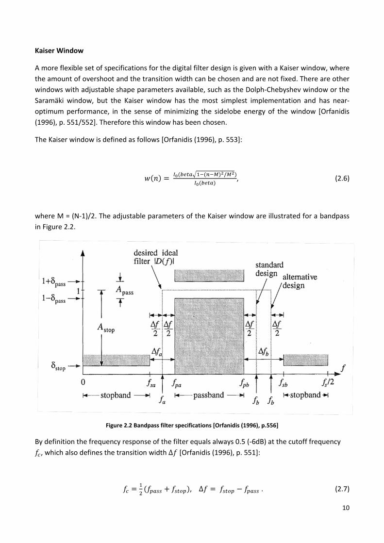
where M = (N-1)/2. The adjustable parameters of the Kaiser window are illustrated for a bandpass in Figure 2.2.

Figure 2.2 Bandpass filter specifications [Orfanidis (1996), p.556]

By definition the frequency response of the filter equals always 0.5 (-6dB) at the cutoff frequency , which also defines the transition width [Orfanidis (1996), p. 551]:

, . (2.7)

11

The passband and stopband overshoots in dB are given by

, . (2.8)

A helpful tool for filter design is the fdatool in MATLAB. The minimum filter order and the filter coefficients are calculated by mainly specifying the transition width, the sampling frequency, the sidelobe attenuation and the type of window. Also the shape parameter beta will be calculated which is another way of expressing the sidelobe attenuation. Higher beta widens the mainlobe and decreases the sidelobe amplitude.

The parameters beta, , , and N are linked with each other by the following equations

[Orfanidis (1996), p. 554]:

0.1102( ), (for ) (2.9)

and

. (2.10)

The transition width has been chosen to be 40 Hz. By requiring an attenuation of = 80 dB this will give N = 5534 number of filter taps and a value of beta = 7.857 results. In turn, by defining beta, N and as stated the implemented function createKaiser.m gives appropriate bandpass filters windowed with a Kaiser window according to the cutoff frequencies specified with transformERB.m by making use of the MATLAB function fir1. The resulting filters are saved in the variable b_vec. The final filters have equal passband and stopband ripples . In the same way the lowpass and the highpass filter are designed by specifying the parameter for the filter type ‘low’ or ‘high’ respectively. The implementation is given by the function createLowHigh.m. Note that the MATLAB function fir1.m automatically creates filters that are 1 tap longer then specified in N, due to the windowing. For the highpass filter N must be an even value.

3. Testing the signal reconstruction

In this part the quality of the signal reconstruction, which is the summation of the individual channels after filterbank processing, is validated.

First of all the feature of a complementary spectrum is proofed. In Figure 3.1 the frequency response of the transfer function of the filterbank is shown in magnitude and phase.

12

Figure 3.1 Magnitude and phase of the filterbank transfer function

The magnitude response shows a flat spectrum around the 0 dB line as expected. A maximum error at low frequencies of 0.01 dB is well below the desirable error of 0.1 dB. The number of bits of N = 5534 are required in order to achieve this low error.

The phase response is linear according to equation (2.5) (with = 0), which results into a constant phase and group delay2

The impulse response reflects directly the filter coefficients and is hence according to the complementary spectrum a delta impulse as verified with Figure 3.2. Note that the system is causal, thus the peak occurs with the above mentioned delay.

of = = -(N-1)/2 = -2767 samples. This feature is only

prevailed when using the same number of filter taps for all filters.

2 The phase delay is defined as the phase response divided by , and the group delay is defined as

the derivative of the phase response with respect to . [Orfanidis (1996), p. 235]

0 0.1 0.2 0.3 0.4 0.5 0.6 0.7 0.8 0.9 1-5

-4

-3

-2

-1

0x 10

5

Normalized Frequency (×π rad/sample)

Pha

se (

degr

ees)

0 0.1 0.2 0.3 0.4 0.5 0.6 0.7 0.8 0.9 1-5

0

5

10

15x 10

-3

Normalized Frequency (×π rad/sample)

Mag

nitu

de (

dB)

Filterbank transfer function

13

Figure 3.2 Impulse response of the filterbank

Furthermore the filterbank has been tested by processing a wav-file (classic1.wav). The original time signal and difference-error that is made after processing are shown in Figure 3.3:

Figure 3.3 Original time-signal and difference-error after processing

The difference-error has a maximum value of 1.8 10-4 and a mean value of -1.76 10-8 with a standard deviation of 3.31 10-5, which is very small. When listening to the processed file no difference to the original file is noticeable.

The chosen order of the filter N is handable for the convolution algorithm in sense of computational costs. For optimising the length of the filter an equiripple FIR design can be chosen, which is optimal in the sense that the maximum error between the desired frequency response and the actual frequency response is minimized.

0.062 0.0625 0.063 0.0635

0

0.2

0.4

0.6

0.8

1X: 0.06277Y: 1

time [s]

Mag

nitu

de

IR of filterbank

0 2 4 6 8 10 12 14-1

-0.8

-0.6

-0.4

-0.2

0

0.2

0.4

0.6

0.8

1wav-file classic1.wav

time[s]

norm

aliz

ed a

mpl

itude

0 2 4 6 8 10 12 140

1

x 10-4 Error between the original and the processed signal

time[s]

abs(

diff

eren

ce in

am

plitu

de)

14

The auditory filterbank is generated by calling the MATLAB function auditoryFilterbank.m (listed in the Appendix) and tests of the filterbank are implemented in testingFilterbank.m

4. Implementation of a single-channel compressor

Compressors and Expanders are dynamic processors and adjust the dynamic range of a signal to that of a post-processing system, for example to the reduced dynamic range of an impaired auditory system. In the following a single-channel feed-forward dynamic range compressor is implemented and then applied to each channel of the filterbank in order to achieve a multi-channel system as commonly used in digital hearing aids.

Compression rule

The operation of the compressor is implemented in two steps according to [Kates (2008), p.227 to 236] and [Orfanidis (1996), p.384 to 388]. First the signal’s level is analyzed by a peak detector (also called level detector) that is then used to calculate the compression gain.

The compression rule describes the compressor’s output as a function of the detector’s output. The attenuation of strong signals is the property of the compressor whereas an expander increases the dynamic range, so that weak signals are attenuated. A limiter and a noise gate are the extreme cases of compression and expansion respectively. Figure 4.1 illustrates the compression rules for the four cases where defines the compression or expansion ratio and x0 the threshold according to equation [Orfanidis (1996), p. 384]:

(4.1)

Figure 4.1 Compression rule for compressor or expander

15

Feedforward implementation of the Automatic Gain Control (AGC)

The automatic gain control (AGC) algorithm is implemented as a feed-forward compression system, as it is typical for digital hearing aids, and is shown in Figure 4.2

Figure 4.2 Block diagram of a compression hearing aid using feed-forward compression control [Kates (2008), p.232]

The volume control for gain positions A,B and C have not been implemented according to the assumption that wide-dynamic-range control sets a comfortable listening level for every sound [Kates (2008), p.231] and are therefore not considered in the analysis.

Peak detector

There are different ways of calculating the detector signal depending of the type of compressor, where the most common ones are [Orfanidis (1996), p. 385]

1. the instantaneous peak value , 2. the root-mean-square value of or 3. the envelope of .

The chosen detector tracks the instantaneous peak value according to [Kates (2008), p. 233]. The detector basically compares in each time step the instantaneous, absolute value of the input signal with the previous detector signal and uses equation 4.2a when the input signal is greater and equation 4.2b in the other case.

(4.2a)

(4.2b)

The difference equation (4.2a) provides a lowpass filter followed by a rectifier and equation (4.2b) is just a low pass filter. The time constant and therefore the cut-off frequency of each lowpass filter can be set with the two parameters attack and release and define the time to rise or fall to a new input level. By definition the attack time constant is the time to rise to a level above the threshold

16

and the release time constant is the time to fall below the threshold, where the threshold indicates the level where the compressor is active.[Orfanidis (1996), p. 385]. For the special case of attack = 0 the detector becomes a pure instantaneous peak detector, which is useful when the compressor is used as a limiter. The level detector provides an adaptive process with equation (4.2a) and (4.2b) as adaptation equation, where the time constant parameters attack and release are the “learning” time constants of the system [Orfanidis (1996), p. 386].

Gain rule

The input to the gain processor is the output of the peak detector and therefore forms the compression rule. The function describing the gain is nonlinear and is given for a compressor

( ) by

(4.3a)

and for an expander ( ) by

, (4.3b)

where d0 is the desired threshold and CR is the general ratio that defines the compression or expansion ratio.

The final output signal of the Compressor is then calculated by multiplying the original input signal x with the estimated gain:

. (4.4)

Possible improvements in the implementation to eliminate some of the overshoots are a delay in the main signal path or an additional lowpass filter that smoothes the nonlinear gain function.

17

These improvements are described in [Orfanidis (1996), p.386] and in [Zölzer (1997), p.211], but have not been implemented in this project.

The single-channel compressor has been implemented as the MATLAB function matrixCompressor.m and is able to process all channels (of the filterbank) at once. It is listed in the Appendix.

5. Analysis of the compressor

The analysis of the dynamic-range compressor comprises the effect of the compressor on input test-signals for a single-channel and for the total system, that is applying the compressor to all channels of the auditory filterbank with uniform parameter settings for the individual channels. In a second step complex audio signals such as music or speech are processed by the system and qualified.

5.1 Analysis of the single – channel dynamic range compressor

Dynamic behavior

In order to ensure correct processing by the single-channel compressor a first analysis is realized according to [Orfanidis (1996), p.386/387]. Therefore a test-signal consisting of three stepped sinusoidal signals, each with a frequency of 2 kHz, is used. The amplitude of the three sinusoids changes from A1 = 2 to A2 = 4 and then to A3 = 0.5. The number of samples is chosen to N = 200 for each sinusoid and the sampling frequency is throughout all following analyses. The threshold of the compressor is d0 = 0.5 and the compressor ratio is with CR = 2, . The attack time is chosen to be attack = 0.9 [Orfanidis (1996), p.386] and the release time release = 0.97 [Kates (2008), p.233]. Figure 5.1.1 shows the input signal, the detector’s output, the gain rule and the compressor output.

18

Figure 4.1.1 Input signal, detector output, gain function and compressor output for attack = 0.9 and release = 0.97

Considering the compressor output it is obvious that the first two sinusoids are compressed because their amplitudes lie above the specified threshold whereas the third sinusoid’s amplitude is unchanged. The attack time and the release time define how fast the detector can track the original signal. This influences the detection in the steady part of the signal as well as in transient parts, that is the abrupt change of amplitude in this case. Considering first the steady part, the detector output does not represent the amplitude of the signal exactly due to the specific set of the time constants. The gain function is obtained by using the detector signal as the input according to equation (4.3a). Therefore this function reflects the opposite movement of the detector when the threshold is passed in a level range from naught to unity and leaves signal parts below the threshold unaffected (gain = 1).

In transient parts of the input signal, that is around n = 200 and n = 400, the influence of the time constants is illustrated in the detector output. Increasing the amplitude abruptly shows the effect of the attack time and the effect of the release time is prominent when the amplitude drops down. By lowering the value of the parameters attack and release the time of the system it takes to react to these changes decreases appropriately. Figure 5.1.2 shows the effect on the

0 100 200 300 400 500 600-4

-3

-2

-1

0

1

2

3

4Input signal

samples n

x(n)

0 100 200 300 400 500 6000

0.5

1

1.5

2

2.5

3

3.5Detector output

samples n

d(n)

0 100 200 300 400 500 6000

0.2

0.4

0.6

0.8

1

Gain

samples n

gain

(n)

0 100 200 300 400 500 600-2

-1.5

-1

-0.5

0

0.5

1

1.5

2compressor output

samples n

y(n)

19

compressor output when lowering one parameter while keeping the value of the other constant. A lower attack time improves the amount of overshoot and a lower release time improves the time to reach the steady state level A3. At the same time lowering the parameters enhances other effects like distortion, where these two parameters also influence each other. It is therefore important to find the right tradeoff between the response time and the introduced distortion [Elliott/Harte (2003), p.17]. This analysis is carried on in the following. The results obtained in this part coincide with those in [Orfanidis (1996), p.386/387] and therefore ensure the correct implementation of the compressor.

The MATLAB function singleCompressor.m comprehends this analysis.

Figure 5.1.2 Compressor output for attack = 0.6 and release = 0.97 (left); attack = 0.9 and release = 0.6 (right)

Estimating the lowpass filter’s time constant

According to [Zölzer (1997), p. 212] the time constant and attack time of a continuous-time system can be found by considering its step response given with

, (5.1)

where is the time constant of the system. The attack time is defined as follows and can be related to the time constant with

, (5.2)

0 100 200 300 400 500 600-1.5

-1

-0.5

0

0.5

1

1.5

2compressor output

samples n

y(n)

0 100 200 300 400 500 600-2.5

-2

-1.5

-1

-0.5

0

0.5

1

1.5

2

2.5compressor output

samples n

y(n)

20

where and declare the times where the signal reaches 90% and 10% of its initial value respectively.

In order to estimate the lowpass filter’s time constant [compare Elliott/Harte (2003), p.14-17] of equation (4.2a) a numerical estimation of this constant has been implemented. Therefore the step function is applied to the compressor with a release parameter of release = 0.97 and a varying attack parameter from 0.01 to 0.99 in 0.01 steps. The result is shown in Figure 5.1.3 (solid line) and links the parameter attack to the time constant . It is remarkable that a attack parameter below 0.6 does not enhance the time constant, but from this value on the time constant increases exponentially.

Figure 5.1.3 Time constant as a function of parameter attack for 3 different step functions

Additionally, two stepped sinusoidal signals with a frequency of 2000 Hz and 100 Hz have also been applied to the compressor in order to proof a dependency of the system on the signal’s frequency. The results are presented in the same Figure. The sinusoid with a high frequency follows the results of the step function whereas the sinusoid with lower frequency results in a time constant that is 9 times higher as in the two other cases. The exponential increase in the time constant for the low frequency signal starts at an attack value of 0.8. The fact that the high-frequency signal follows the results of the step function underlines that the detector follows the envelope of the signal for high frequencies whereas it follows the fine structure for low frequency components. Hence, the frequency of the signal is an additional parameter that influences the dynamics of the system. A similar analysis can be done for the release parameter, where an inversed step that jumps from 1 to 0 has to be applied.

0 0.1 0.2 0.3 0.4 0.5 0.6 0.7 0.8 0.9 10

0.1

0.2

0.3

0.4

0.5

0.6

0.7

0.8

0.9

1x 10

-3 Low-pass filter´s time constant TL as a function of the parameter attack

attack (parameter)

time

cons

tant

TL

[s]

step functionstepped sinusoid with f = 2000 Hzstepped sinusoid with f = 100 Hz

21

Nonlinear Distortion

The nonlinear distortion introduced by the compressor is mainly harmonic distortion as it is shown in the following. Harmonic distortion refers to the property of the system to generate harmonics when a pure tone is applied to the system. Harmonic distortion is most easily studied in a power series representation, where the output y(t) is related to the input x(t) by

. (5.3)

The first term refers to a linear system in the case where only this term is present. All harmonics are possible in the output when both even and odd powers of the input are contained in the power series and no specific symmetry can be obtained in this case. The spectrum contains just even-numbered harmonics for a even-numbered power series and introduces also a DC term to the output. In the case where the system has only odd powers in the power series, accordingly only odd-number harmonics will occur in the spectrum and no DC term arises. The phase of the sinusoidal signal is not important in harmonic distortion described by a power series.

The power series is a memoryless representation of a nonlinear input-output characteristic and therefore does not account for linear filters, such as a lowpass filter, in which case the output depends on the input at previous times. The latter case refers to the dynamical representation of nonlinear distortion. For gross nonlinearities such as half-wave rectification the power series representation is not a good model of choice. [Hartmann (1998), p.491-497]

The origin of nonlinear distortion in the present compressive system are in a first stage introduced by the peak detector since wave rectification (absolute value of the input signal), that introduces spectral splatter due to the sharp transitions in the time signal after the rectification, and lowpass filterering are applied to the signal. In a second stage the gain rule describes a nonlinear compressive function.

The analysis of the nonlinear distortion focuses on the numerical estimation of the total harmonic distortion and therefore no comparison to a model study will be done in the frame of this project.

Total harmonic distortion (THD)

As already mentioned by decreasing the time constants the distortion of the compressor on the input signal will be increased. The degree of distortion can be quantified with the total harmonic distortion that is defined as [Elliott/Harte (2003), p.6]

22

. (5.4)

The total harmonic distortion of the automatic gain control system has been estimated by applying a pure tone (sinusoid with a frequency of 2 kHz and an amplitude of A = 2) of steady amplitude to the system. The spectra of the input signal x(t) and the output y(t) are evaluated at a steady part of the signal, that means in a part where overshoots are completely declined and no longer present. The power spectrum after the compression is then used, by identifying the peaks, to calculate the THD according to equation (5.4). The parameter settings of the compressor are unchanged to the previous ones. Figure 5.1.4 illustrates the power spectra of each stage of the compressor.

Figure 5.1.4 Powerspectra of the different stages of the AGC

The first spectrum shows the ideal sinusoid at 2 kHz at 6 dB with a noise floor of -300 dB (internal machine noise is not shown in the graph). Considering the signal after compression the

0 0.5 1 1.5 2

x 104

-100

-90

-80

-70

-60

-50

-40

-30

-20

-10

0

10

frequency [Hz]

Mag

nitu

de in

dB

Powerspectrum of the signal

0 0.5 1 1.5 2

x 104

-100

-90

-80

-70

-60

-50

-40

-30

-20

-10

0

10

frequency [Hz]

Mag

nitu

de in

dB

Powerspectrum of the detector output

0 0.5 1 1.5 2

x 104

-100

-90

-80

-70

-60

-50

-40

-30

-20

-10

0

10

frequency [Hz]

Mag

nitu

de in

dB

Powerspectrum of the gain

0 0.5 1 1.5 2

x 104

-100

-90

-80

-70

-60

-50

-40

-30

-20

-10

0

10

frequency [Hz]

Mag

nitu

de in

dB

Powerspectrum of the signal after compression

23

fundamental frequency is unchanged at 2 kHz with a reduced amplitude of 1.5 dB. In addition to the fundamental frequency odd-number harmonics corresponding to odd powers of the input in the power series of equation (5.3) are generated with decaying amplitude. Another effect that is prominent is the amplitude modulation of the signal indicated by the sidebands placed with a distance of ± (modulation frequency) from each harmonic with a reduced amplitude. The spectrum of the gain function is a compressed version in amplitude of the spectrum of the detector output. It is remarkable that the fundamental frequency is missing in these two plots and just even-numbered harmonics are present. This is due to the wave rectification applied in the peak detector. The rectification can be seen as a doubling in frequency and therefore only even-number harmonics occur. There is also a peak at f = 0 Hz corresponding to the DC term that is always accompanied with this (even) kind of power series. Since the output signal is obtained by multiplying the input signal with the gain function in the time domain, this corresponds to a convolution in the frequency domain and hence the output spectrum is obtained by convolving the input spectrum with the gain spectrum. This operation shifts the spectrum of the gain function about ones the fundamental frequency, thus the resulting output spectrum contains odd-numbered harmonics. The regions between the harmonics can be interpreted as an increased noise floor, but by looking closer these areas represent a regular pattern, so that they can also be interpreted as weak even-number harmonics that are also introduced and accompanied by amplitude modulation.

THD as a function of amplitude

It is now interesting to know how the total harmonic distortion changes as a function of the amplitude of the signal. Therefore a 2 kHz - sinusoid and a 100 Hz - sinusoid are used by varying them in amplitude from A = 0.1 to 2 in 0.1 steps. The results are presented in Figure 5.1.5.

Figure 5.1.5 THD of a sinusoid with f = 2 kHz (left graph) and with f = 100 Hz (right graph) varying the amplitude from A = 0.1 to 2.

0 0.2 0.4 0.6 0.8 1 1.2 1.4 1.6 1.8 20

0.5

1

1.5

2

2.5

Amplitude

TH

D [

%]

THD as function of amplitude

0 0.2 0.4 0.6 0.8 1 1.2 1.4 1.6 1.8 20

2

4

6

8

10

12

14

16

18

Amplitude

THD

[%

]

THD as function of amplitude

24

As expected there is no distortion below the threshold of d0 = 0.5 in both cases. Above this threshold the THD increases fast to a constant value of 2.1 % irrespective of further increase of the amplitude for the high frequency signal. The low frequency signal converges steadily to a THD of 16 %. Therefore it can be stated that low frequency signals generate much higher distortion than high frequency components.

This analysis is available in the MATLAB script singleCompressor_steady_THD.m

THD as a function of attack time or release time

The afore introduced change of the time constants influences the total harmonic distortion. This is illustrated in the following four graphs in Figure 5.1.6, where one parameter is varied for two different constant values of the other parameter. The used test signals are two sinusoids with frequency 2 kHz and 100 Hz both with a amplitude of A = 2.

Figure 5.1.6 THD as a function of parameter attack (left plots: release = 0.97 (upper plot), release = 0.5 (lower plot)) or release (right plots: attack = 0.9 (upper plot), attack = 0.5 (lower plot)) for a 2 kHz – sinusoid (solid line) and a 100 Hz – sinusoid (dashed line).

0 0.1 0.2 0.3 0.4 0.5 0.6 0.7 0.8 0.9 10

2

4

6

8

10

12

14

16

18

attack time (parameter)

THD

[%

]

THD as function of attack time

0 0.1 0.2 0.3 0.4 0.5 0.6 0.7 0.8 0.9 10

2

4

6

8

10

12

14

16

18

release time (parameter)

TH

D [

%]

THD as function of release time

0 0.1 0.2 0.3 0.4 0.5 0.6 0.7 0.8 0.9 10

2

4

6

8

10

12

14

16

18

20

attack time (parameter)

THD

[%

]

THD as function of attack time

0 0.1 0.2 0.3 0.4 0.5 0.6 0.7 0.8 0.9 10

5

10

15

20

25

release time (parameter)

THD

[%

]

THD as function of release time

25

For the high frequency signal in general the THD decreases when the appropriate time constant parameter is increased. By setting one value to 0.5 results in a very high distortion (up to 20 %) when also the other parameter is lowered. For the lower left graph the THD even decreases again from its maximum value at 0.5 (18 %) of around 2 %. For the low frequency signal the THD is constant of 15 % to 17 % up to a parameter value of release = 0.97 (right graphs) and attack = 0.8 (left graphs) before the curve drops down. The left graphs show a peak value that is 3 % higher (18%) than the constant value before the curve drops. By comparing the different frequencies the low frequency arises in general much higher distortion, which is in agreement with the previous observations. A high frequency signal generates higher distortion for a low constant time parameter below a value of around 0.7 (lower right graph: up to 23 %) to 0.8 (lower left graph).

As can be seen from Figure 5.1.3 it is pointless to choose an attack parameter below 0.6 for high frequency signals, since below these values the time constant of the system is not improved. On the other hand for low frequency signals the time constant parameter should be chosen below 0.8 since the distortion can have a peak above this value and also the time constant is lowered. A good set of parameters is found for attack = 0.6 and release = 0.97 with a resulting total harmonic distortion of under 5 % for high frequencies. These graphs describe a tendency of the system for low and high frequencies, but since this system is nonlinear the full frequency range should be analyzed with all different combinations of time constant parameters in order to ensure these tendencies. The analysis of this part is implemented in the MATLAB function singleCompressor_steady_THD_att.m.

5.2 Analysis of the multi – channel dynamic range compressor

In this part the single-channel dynamic compressor is applied to all channels with uniform parameter settings in each individual channel, so that the complete digital signal processing system of a multi-channel dynamic range compressor is achieved. The resulting system is implemented in mainMultiCompressor.m that calls all relevant functions and is listed in the Appendix.

The analysis of the multi-channel compressor is carried on according to the analysis in [Kates (2008), p.236-241]

26

ANSI test

The first test uses a standardized ANSI test signal according to ANSI S3.22 (2003) test for compression dynamic behavior. The test signal is stepped sinusoidal signal with a frequency of 2 kHz and jumps 35 dB in amplitude after 200 ms and returns to the original level at 500 ms. This test signal is implemented in the MATLAB function inputANSI.m. The test signal is applied to the multi-channel system with attack = 0.65, release = 0.97 and CR = 2 and the results are shown in Figure 5.2.1.

Figure 5.2.1 Different stages of the multi-channel compressor for the ANSI S3.22 (2003) test signal

The most prominent observation is the overshoots at both sides of the step of the output of the compressor as well as in the output of the detector. The spikes at the transition areas are the in [Kates (2008), p.238] described consequences at other frequencies caused by the change in amplitude in one band. The multi-channel compression amplifies the out-of-band transients. The jump in amplitude generates a large amount of spectral content in other frequency bands that is than amplified by the high gain in these channels that was established for the low initial input levels.

0 0.1 0.2 0.3 0.4 0.5 0.6 0.7-40

-30

-20

-10

0

10

20

30

40Input signal

time (s)

x(n)

0 0.1 0.2 0.3 0.4 0.5 0.6 0.70

0.2

0.4

0.6

0.8

1

1.2

1.4Detector output

time (s)

d(n)

0 0.1 0.2 0.3 0.4 0.5 0.6 0.70.99

0.992

0.994

0.996

0.998

1

1.002Gain

time (s)

gain

(n)

0 0.1 0.2 0.3 0.4 0.5 0.6 0.7-40

-30

-20

-10

0

10

20

30

40compressor output

time (s)

y(n)

27

Chirp test

The second test uses a swept sinusoid starting at 200 Hz up to 8 kHz and has a duration of 3 ms. This test refers to [Kates (2008), p.240/241]. The compressor settings are unchanged to the previous test and the result is presented in Figure 5.2.2.

Figure 5.2.2 Multi-channel compressor output for a swept sinusoid

The obtained peaks are due to filter gain at the band edges interacting with the compression amplification as described in [Kates (2008), p.240]. The filters have a gain of -6 dB at their edges. Therefore a signal is attenuated. By adding all channels consecutive channels compensate for this attenuation, but only if no compression is applied. In this case there is additional compressor gain in the edges of the filters and therefore increases the amplitude of the signal at these areas. The peaks correspond to a level difference of 2.5 dB.

Processing a wav-file

The last test uses a music signal (gspi.wav). The file contains a recording of a simple melody played on a glockenspiel and therefore has a time signal with sharp impulsive components. The different stages of the multi-channel compressor are presented in Figure 5.2.3.

An extreme setting of parameters has to be chosen for the compressor in order to achieve a gain-function apart from unity. These settings are attack = 0.1, release = 0.97, CR = 4 and d0 = 0.01. When listening to the processed file no distortion is audible. When the release time is also decreased a high degree of distortion is observed at the impulses, due to the fact that the glockenspiel contains high

0 0.5 1 1.5 2 2.5 3-1.5

-1

-0.5

0

0.5

1

1.5compressor output

time (s)

y(n)

28

frequency components, which fits to the previous observations. The processing time for such a high quality recording (16 bits, 44.1 kHz, duration: 6 s) is about 38 seconds.

Figure 5.2.3 Different stages of the multi-channel compressor for the wav-file gspi.wav

6. Conclusion In this project a multi-channel dynamic-range compressor has been implemented and analysed. The analysis of the system has been applied on the basis of [Kates (2008), pp. 221-241], [Elliott and Harte (2003), pp. 1-23] and [Orfanidis (1996), chapter 10 and pp. 384-388] and well-known properties of the system could be verified and outlined. The auditory filterbank comprises 37 channels depending on the specified frequency range, where the bandpass filers are critical band wide and are adjoined by a lowpass and a highpass filter at the edges of the spectrum. The chosen filter design method uses Kaiser windows with a uniform

0 1 2 3 4 5 6-1

-0.8

-0.6

-0.4

-0.2

0

0.2

0.4

0.6

0.8

1Input signal

time (s)

x(n)

0 1 2 3 4 5 60

0.005

0.01

0.015

0.02

0.025

0.03

0.035

0.04

0.045Detector output

time (s)d(

n)

0 1 2 3 4 5 6

0.65

0.7

0.75

0.8

0.85

0.9

0.95

1Gain

time (s)

gain

(n)

0 1 2 3 4 5 6-1

-0.8

-0.6

-0.4

-0.2

0

0.2

0.4

0.6

0.8

1Input signal

time (s)

x(n)

29

number of samples of N = 5534 samples in order to achieve a linear phase response and a signal reconstruction with an error of 0.01 dB. The analysis of the single-channel compressor shows the tradeoff between a fast attack time constant and the resulting total harmonic distortion. The influence of the time constants on each other as well as the additional influence of the signals frequency have been outlined and illustrated by varying these parameters. In future work it would be interesting to make a full 2 dimensional analysis of the two parameters attack and release for all possible combinations in the whole frequency range in order to ensure the tendencies of the system that have been evaluated.

References

[1] Breebaart, J, (2001). “Modeling binaural signal detection”. PhD thesis, Technical University of Eindhoven, the Netherlands.

[2] Kates, J. M. (2008). “Digital Hearing Aids”. Plural Publishing, San Diego.

[3] Elliott, S. J. and Harte, J. M. (2003). “Models for Compressive Nonlinearities in the Cochlea”. Report from the Institute of Sound and Vibration Research, University of South Hampton.

[4] Zölzer, U. (1997). ”Digital Audio Signal Processing”. John Wiley & Sons, Inc.

[5] Sophocles J., Orfanidis (1996). ”Introduction to Signal Processing”. Prentice-Hall, Inc., New Jersey.

[6] Hartmann, William M. (1998). “Signals, Sound and Sensation”. Springer-Verlag New York, Inc.

30

List of Figures

Figure 2.1 Illustration of the filterbank, p.8

Figure 2.2 Bandpass filter specifications [Orfanidis (1996), p.556], p.10

Figure 3.2 Magnitude and phase of the filterbank transfer function, p.12

Figure 3.3 Impulse response of the filterbank, p.13

Figure 3.4 Original time-signal and difference-error after processing, p.13

Figure 4.1 Compression rule for compressor or expander, p.14

Figure 4.2 Block diagram of a compression hearing aid using feed-forward compression control [Kates (2008), p.232], p.15

Figure 5.1.1 Input signal, detector output, gain function and compressor output for attack = 0.9 and release = 0.97, pp. 17-18

Figure 5.1.3 Time constant as a function of parameter attack for 3 different step functions, p.20

Figure 5.1.4 Power spectra of the different stages of the AGC, p.22

Figure 5.1.5 THD of a sinusoid with f = 2 kHz (left graph) and with f = 100 Hz (right graph) varying the amplitude from A = 0.1 to 2, p.23

Figure 5.1.6 THD as a function of parameter attack (left plots: release = 0.97 (upper plot), release = 0.5 (lower plot)) or release (right plots: attack = 0.9 (upper plot), attack = 0.5 (lower plot)) for a 2 kHz – sinusoid (solid line) and a 100 Hz – sinusoid (dashed line), p.24

Figure 5.2.1 Different stages of the multi-channel compressor for the ANSI S3.22 (2003) test signal, p.26

Figure 5.2.2 Multi-channel compressor output for a swept sinusoid, p.27

Figure 5.2.3 Different stages of the multi-channel compressor for the wav-file gspi.wav, pp.28

31

Appendix %transformERB.m function f0 = transformERB(f_low,f_high) %Transforms the frequency domain into the ERB-frequency-domain z_low = 1/.11*log(.00437*f_low+1); %f_low-frequency transformed to ERB-scale z_high = 1/.11*log(.00437*f_high+1); %f_high-frequency transformed to ERB-scale z0 = z_low:1:z_high; %one auditory filter per ERB (linear distribution of filters

on ERB-scale) f0 = (exp(0.11*z0)-1)/.00437; %frequency vector in [Hz] %EOF %createKaiser.m %Creates a bandpass with specified parameters; window: Kaiser function filter = createKaiser(Fs,N,Fc1,Fc2) % Fs: Sampling Frequency % N: Order % Fc1: First Cutoff Frequency % Fc: Second Cutoff Frequency flag = 'scale'; % Sampling Flag Beta = 7.857; % Window Parameter % Create the window vector for the design algorithm. win = kaiser(N+1, Beta); % Calculate the coefficients using the FIR1 function. filter = fir1(N, [Fc1 Fc2]./(Fs/2), 'bandpass', win, flag); % [EOF] %createLowHigh.m %Creates either a lowpass or a highpass filter dependend on specified %parameters; window: Kaiser function filter = createLowHigh(Fs,N,Fc,wintype) % Fs: Sampling Frequency % N: Order % Fc: Cutoff Frequency % wintype: highpass('high')/lowpass('low') flag = 'scale'; % Sampling Flag Beta = 7.857; % Window Parameter % Create the window vector for the design algorithm. win = kaiser(N+1, Beta); % Calculate the coefficients using the FIR1 function. filter = fir1(N, Fc/(Fs/2), wintype, win, flag);

32

%%%%%%%%%%%%%%%%%%%%%%%%%%%%%%%%%%%%%%%%%%%%%%%%%%%%%%%%%%%%%%%%%%%%%%%%%%%% %% Implementation and analysis of a multi-channel dynamic-range compressor % %%%%%%%%%%%%%%%%%%%%%%%%%%%%%%%%%%%%%%%%%%%%%%%%%%%%%%%%%%%%%%%%%%%%%%%%%%%% % by Johannes Käsbach, DTU, Acoustic Technology, June 2009 %% Part 1: Auditory Filterbank %auditoryFilterbank.m %This file creates an auditory filterbank where the bandwidth of the %filters corresponds to one ERB function fbank = auditoryFilterbank(fs,N,beta,range) % %Definitions % fs = 44100; %Sampling frequency [Hz] % N = 5534; %Number of filter taps (order of the filter) % beta = 7.857; %defining the sidelobes % range = [100 16000]; %lower and upper limit of bandpass filters %Implementation %center-frequencies and ERB-bandwidths f0 = transformERB(range(1),range(2)); %gives the cut-off frequencies of the bands. f0's are exactly one ERB spaced %lower and upper cut-off-frequency (according to Orfandis, p.556) fa = round(f0(1,1:end-1)); fb = round(f0(1,2:end)); %Calculate a ERB-wide bandpass-filter(window: Kaiser) for all channels channels = length(fa); %Number of channels;length(f0)-1 band_vec = zeros(N+1,channels); %Allocation for ch = 1 : channels band_vec(:,ch) = createKaiser(fs,N,fa(1,ch),fb(1,ch),beta); end %Calculate a low-pass filter at the low-frequency limit of the %filterbank spectrum fc_low = fa(1); lowpass(:,1) = createLowHigh(fs,N,fc_low,beta,'low'); %Calculate a high-pass filter at the upper-frequency limit of the %filterbank spectrum fc_high = fb(end); highpass(:,1) = createLowHigh(fs,N,fc_high,beta,'high'); %the complete auditory filterbank fbank = [lowpass band_vec highpass]; %[EOF]

33

%%%%%%%%%%%%%%%%%%%%%%%%%%%%%%%%%%%%%%%%%%%%%%%%%%%%%%%%%%%%%%%%%%%%%%%%%%%% %% Implementation and analysis of a multi-channel dynamic-range compressor % %%%%%%%%%%%%%%%%%%%%%%%%%%%%%%%%%%%%%%%%%%%%%%%%%%%%%%%%%%%%%%%%%%%%%%%%%%%% % by Johannes Käsbach, DTU, Acoustic Technology, June 2009 %% Part 2: Single-channel compressor %matrixCompressor.m %This file creates a single channel compressor using feed-forward %compression control that can be applied by each channel of the %auditory filterbank (auditoryFilterbank.m) function [d gain y] = matrixCompressor(x,fs,attack,release,CR,thresh) %Definitions % x: input signal (N x channels) % fs: Sampling frequency in [Hz] % attack: attack time constant (fast) /forgetting factor % release: release time constant (slow) % CR: Compressor ratio d0 = thresh; %threshold %%peakDetector % x(n): input signal % d(n): peak detector output %%Compressor, Limiter, Expander and Gates [Orfanidis p.384-388] % gain(n): nonlinear time dependent gain % y(n): compressor output %Implementation %peak detector algorithm: adaptation equation d = zeros(size(x)); %Allocation [N_dim ch] = size(x); for n = 1 : (N_dim-1) A = (abs(x(n+1,:))>= d(n,:)); %if-statement case1 = attack*d(n,:)+(1-attack).*abs(x(n+1,:));%A is true case0 = release*d(n,:); %A is false d(n+1,:) = A.*case1 + (1-A).*case0; %adaptation equation end gain = zeros(size(x)); %Allocation y = zeros(size(x)); %Allocation for n = 1 : N_dim %Compressor(roh <1) roh = 1/CR; % %Limiter(roh <<1) % roh = 1/10; A = d(n,:)>= d0; case1 = (d(n,:)/d0+1e-15).^(roh-1); case0 = 1; gain(n,:) = A.*case1 +(1-A).*case0;

34

%Expander(roh >1) % roh = CR; % %Gate(roh>> 1) % %roh = 10; % B = d(n,:) <= d0; % gain(n,:) = B.*case1 +(1-B).*case0; %compressor output y(n,:) = gain(n,:).*x(n,:); end %shift vectors by 1 sample because detector starts at d(n+1,:) d = d(2:end,:); gain = gain(2:end,:); y = y(2:end,:); % [EOF] %%%%%%%%%%%%%%%%%%%%%%%%%%%%%%%%%%%%%%%%%%%%%%%%%%%%%%%%%%%%%%%%%%%%%%%%%%%% %% Implementation and analysis of a multi-channel dynamic-range compressor % %%%%%%%%%%%%%%%%%%%%%%%%%%%%%%%%%%%%%%%%%%%%%%%%%%%%%%%%%%%%%%%%%%%%%%%%%%%% % by Johannes Käsbach, DTU, Acoustic Technology, June 2009 %% Part 1 + Part 2: Multi-channel Compressor %mainMultiCompressor.m %This file generates an multi-channel dynamic-range compressor by %first generating an auditory filterbank (Part 1: auditoryFilterbank.m) and %then applying a single-channel compressor to each channel (Part 2 : singleCompresssor.m) %Finally all channels are added up. %Individual tests of the Filterbank and the Compressor are available under %testingFilterbank.m and testingCompressor.m respectively clc; clear all; close all; tic %start measuring total simualation time %Input signals %1) stepped sinusoid fs = 44100; %Sampling frequency [Hz] % % a) Orfanidis test-signal p.386 % f_sin = 2000; %[Hz] % N_sin = 200; % t = (1 : 1 : N_sin)/fs; % x1 = 2*sin(2*pi*f_sin*t); % x2 = 4*sin(2*pi*f_sin*t); % x3 = 0.5*sin(2*pi*f_sin*t); % xd = 0.5*sin(2*pi*f_sin*[N_sin+1 N_sin+2]/fs); % x = [x1 x2(1,1:end-2) x3 xd]';

35

% % b) ANSI S3.22(2003) test for compression dynamic behaviour 30dB-jump in level % [x t] = inputANSI(fs); % % 2) delta-pulse % delta = [1 zeros(1,length(t)-1)]; % x = delta; % 3) wav-file [wav_file,fs_read,nbits]= wavread('gspi.wav'); [N_wav ch_wav] = size(wav_file); t = (1:1:N_wav)/fs_read; x = wav_file; % % 4)Chirp % F0 = 200; % F1 = 8000; % T1 = 3; % N_sig = fs*T1; %signal's number of samples % t = (1:1:N_sig)/fs; %time vector of the signal % x = chirp(t,F0,T1,F1)'; %%Part 1: Generate an auditory Filterbank N = 5534; %Number of filter taps (order of the filter) N_equi = 2176; beta = 7.857; %defining the sidelobes delta_f = 30; %delta f around cutoff frequ in [Hz] range = [100 16000]; %frequency-range of the filterbank's bandpass filters x_new = [x; zeros(N/2,1)]; filterbank = auditoryFilterbank(fs,N,beta,range); %filterbank_equi = auditoryFilterbankEquiripple(fs,N_equi,delta_f,range); %%Testing the signal reconstruction of the filterbank %testingFilterbank(filterbank,fs,N); %Filter the input signal with the auditory filterbank [dim_N channels] = size(filterbank); xfilt = fftfilt(filterbank,x_new); %xfilt_exc = xfilt((N/2+1):end,:); xfilt = xfilt(N/2:end,:); %%Part 2: Generate the multi-channel dynamic-range compressor %Paramters for Compressor (normal) % attack = 0.6; %attack time constant (fast) /forgetting factor % release = 0.97; %release time constant (slow) % CR = 2; %Compressor ratio % thresh = 0.5; %threshold %Parameters for Compressor (Glockenspiel) attack = 0.1; %attack time constant (fast) /forgetting factor release = 0.4; %release time constant (slow) CR = 4; %Compressor ratio thresh = 0.01; %threshold

36

[d_vec gain_vec y_vec] = matrixCompressor(xfilt,fs,attack,release,CR,thresh); %Add all channels d_total = sum(d_vec,2)/channels; gain_total = sum(gain_vec,2)/channels; y_total = sum(y_vec,2); %y_total = y_total(2:end,:); %plots %t_plot = (1 : 1 : 3*N_sin)/fs; t_plot = t; plot(t_plot,x) title('Input signal'),xlabel('time (s)'),ylabel('x(n)'); figure plot(t_plot,d_total) title('Detector output'),xlabel('time (s)'),ylabel('d(n)'); figure plot(t_plot,gain_total) title('Gain'),xlabel('time (s)'),ylabel('gain(n)'); figure plot(t_plot,(y_total)) title('compressor output'),xlabel('time (s)'),ylabel('y(n)'); %individual bands figure plot(t_plot,y_vec(:,2),'b') hold plot(t_plot,y_vec(:,18),'r') plot(t_plot,y_vec(:,26),'gr') title('compressor output'),xlabel('time (s)'),ylabel('y(n)'); simtime = toc; %stop measuring total simulation time %and save it in simtime %[EOF]