Implementation of a Hardware Coordinate Wise Descend

Master of Science Thesis in Electrical EngineeringDepartment of Electrical Engineering, Linköping University, 2020

Implementation of aHardware Coordinate WiseDescend Algorithm withMaximum LikelihoodEstimator for Use in mMTCActivity Detection

Mikael Henriksson

Master of Science Thesis in Electrical Engineering

Implementation of a Hardware Coordinate Wise Descend Algorithm withMaximum Likelihood Estimator for Use in mMTC Activity Detection:

Mikael Henriksson

LiTH-ISY-EX–20/5326–SE

Supervisor: Oscar Gustafssonisy, Linköpings universitet

Examiner: Mattias Krysanderisy, Linköpings universitet

Division of Computer EngineeringDepartment of Electrical Engineering

Linköping UniversitySE-581 83 Linköping, Sweden

Copyright © 2020 Mikael Henriksson

Abstract

In this work, a coordinate wise descent algorithm is implemented which servesthe purpose of estimating active users in a base station/client wireless communi-cation setup. The implemented algorithm utilizes the sporadic nature of users,which is believed to be the norm with 5G Massive MIMO and Internet of Things,meaning that only a subset of all users are active simultaneously at any giventime. This work attempts to estimate the viability of a direct algorithm imple-mentation to test if the performance requirements can be satisfied or if a moresophisticated implementation, such as a parallelized version, needs to be created.

The result is an isomorphic ASIC implementation made in a 28 nm FD-SOIprocess, with proper internal word lengths extracted through simulation. Sometechniques to lessen the burden on hardware without losing performance is pre-sented which helps reduce area and increase speed of the implementation. Fi-nally, a parallelized version of the algorithm is proposed, if one should desire toexplore an implementation with higher system throughput, at almost no furtherexpense of user estimation error.

iii

Acknowledgments

A huge thank you to my supervisor Oscar Gustafsson, who on multiple occasionshelped me back on the right track when I was lost and who always deliveredfantastic feedback.

I would also like to thank Petter Källström and Frans Skarman for letting mebug you with my stupid ideas.

Linköping, May 2020

v

Contents

1 Introduction 11.1 Motivation . . . . . . . . . . . . . . . . . . . . . . . . . . . . . . . . 21.2 Purpose . . . . . . . . . . . . . . . . . . . . . . . . . . . . . . . . . . 21.3 Research issue . . . . . . . . . . . . . . . . . . . . . . . . . . . . . . 21.4 Delimitations . . . . . . . . . . . . . . . . . . . . . . . . . . . . . . . 3

2 Theory 52.1 Notation . . . . . . . . . . . . . . . . . . . . . . . . . . . . . . . . . 52.2 Terminology . . . . . . . . . . . . . . . . . . . . . . . . . . . . . . . 5

2.2.1 Performance terms . . . . . . . . . . . . . . . . . . . . . . . 62.2.2 Hardware terms . . . . . . . . . . . . . . . . . . . . . . . . . 62.2.3 Other terms . . . . . . . . . . . . . . . . . . . . . . . . . . . 6

2.3 Studied scenario . . . . . . . . . . . . . . . . . . . . . . . . . . . . . 72.4 The problem . . . . . . . . . . . . . . . . . . . . . . . . . . . . . . . 82.5 Algorithm to implement . . . . . . . . . . . . . . . . . . . . . . . . 9

2.5.1 Updating the variance estimate . . . . . . . . . . . . . . . . 92.5.2 Performance requirements . . . . . . . . . . . . . . . . . . . 9

2.6 Hardware aspects of implementation . . . . . . . . . . . . . . . . . 102.6.1 Numeric representation . . . . . . . . . . . . . . . . . . . . 102.6.2 Word length . . . . . . . . . . . . . . . . . . . . . . . . . . . 102.6.3 Combinational latency . . . . . . . . . . . . . . . . . . . . . 112.6.4 Critical path . . . . . . . . . . . . . . . . . . . . . . . . . . . 112.6.5 Critical loop . . . . . . . . . . . . . . . . . . . . . . . . . . . 112.6.6 Isomorphic implementation . . . . . . . . . . . . . . . . . . 13

3 Results of isomorphic implementation 153.1 Models . . . . . . . . . . . . . . . . . . . . . . . . . . . . . . . . . . 15

3.1.1 MATLAB model . . . . . . . . . . . . . . . . . . . . . . . . . 163.1.2 C++ model using floating-point arithmetic . . . . . . . . . 173.1.3 C++ model using fixed-point arithmetic . . . . . . . . . . . 183.1.4 RTL VHDL model . . . . . . . . . . . . . . . . . . . . . . . . 18

3.2 Sequence . . . . . . . . . . . . . . . . . . . . . . . . . . . . . . . . . 183.2.1 Random sequences with memories . . . . . . . . . . . . . . 18

vii

viii Contents

3.2.2 Pseudo random modulo sequence . . . . . . . . . . . . . . . 203.3 Implementation flow graphs . . . . . . . . . . . . . . . . . . . . . . 213.4 Verification . . . . . . . . . . . . . . . . . . . . . . . . . . . . . . . . 213.5 Word length simulations . . . . . . . . . . . . . . . . . . . . . . . . 23

3.5.1 Integer bits . . . . . . . . . . . . . . . . . . . . . . . . . . . . 233.5.2 Fractional bits . . . . . . . . . . . . . . . . . . . . . . . . . . 24

3.6 Synthesis . . . . . . . . . . . . . . . . . . . . . . . . . . . . . . . . . 243.7 Conclusion . . . . . . . . . . . . . . . . . . . . . . . . . . . . . . . . 24

4 Investigation of parallel algorithm 274.1 Parallel execution . . . . . . . . . . . . . . . . . . . . . . . . . . . . 274.2 Reducing the size of matrix inverse in parallel coordinate descent 284.3 Flowgraphs for Woodbury architecture . . . . . . . . . . . . . . . . 314.4 Conclusion . . . . . . . . . . . . . . . . . . . . . . . . . . . . . . . . 31

5 Conclusion and final remarks 335.1 Algorithms . . . . . . . . . . . . . . . . . . . . . . . . . . . . . . . . 335.2 Implementation . . . . . . . . . . . . . . . . . . . . . . . . . . . . . 33

A Wordlength simulations 37

B Initial MATLAB model 41B.1 File: "GenerateBinarySequence.m" . . . . . . . . . . . . . . . . . . . 41B.2 File: "ComputePfaPmd.m" . . . . . . . . . . . . . . . . . . . . . . . 41B.3 File: "GenerateComplexGaussian" . . . . . . . . . . . . . . . . . . . 42B.4 File: "CoordinateDescend_AD_ML_Fast.m" . . . . . . . . . . . . . 42B.5 File: "CoordinateDescent.m" . . . . . . . . . . . . . . . . . . . . . . 43

Bibliography 45

1Introduction

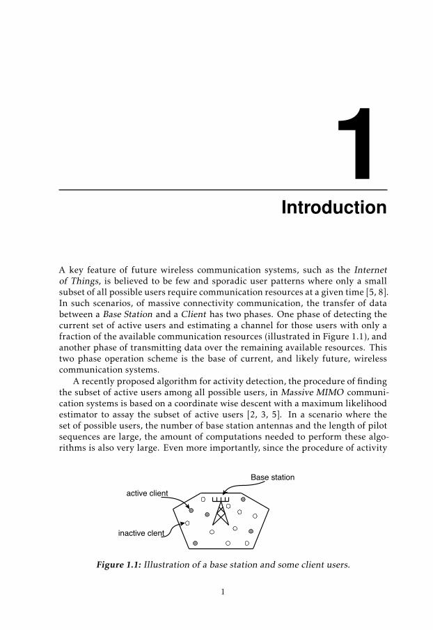
A key feature of future wireless communication systems, such as the Internetof Things, is believed to be few and sporadic user patterns where only a smallsubset of all possible users require communication resources at a given time [5, 8].In such scenarios, of massive connectivity communication, the transfer of databetween a Base Station and a Client has two phases. One phase of detecting thecurrent set of active users and estimating a channel for those users with only afraction of the available communication resources (illustrated in Figure 1.1), andanother phase of transmitting data over the remaining available resources. Thistwo phase operation scheme is the base of current, and likely future, wirelesscommunication systems.

A recently proposed algorithm for activity detection, the procedure of findingthe subset of active users among all possible users, in Massive MIMO communi-cation systems is based on a coordinate wise descent with a maximum likelihoodestimator to assay the subset of active users [2, 3, 5]. In a scenario where theset of possible users, the number of base station antennas and the length of pilotsequences are large, the amount of computations needed to perform these algo-rithms is also very large. Even more importantly, since the procedure of activity

Base station

inactive clent

active client

Figure 1.1: Illustration of a base station and some client users.

1

2 1 Introduction

detection in a wireless communication system should only use a fraction of theavailable communication resources, coherence time being one such resource, thedemand for low latency execution is of importance.

To the authors knowledge, there are only two earlier publications [11, 13] im-plementing activity detection algorithms for use in massive machine type com-munication. However, their use case are somewhat different from this imple-mentation, making it difficult to directly compare performance between theseimplementations.

1.1 Motivation

The gap between a mathematical representation of an algorithm and its hardwareimplementation is not always trivial to bridge. The sheer amount of arithmeticcomputations and the algorithms degree of parallelism can limit the desired per-formance of an algorithmic implementation. By attempting to implement themathematical algorithm in hardware, the difficulties of implementation will man-ifest themselves which have the possibility to extend the bridge between mathe-matically rigorous algorithms and implementation-wise reasonable algorithms.Figure 1.2 illustrates the process of taking a mathematical representation of analgorithm to tape out of an application specific integrated circuit.

1.2 Purpose

This work serves the purpose of making a draft implementation of a new activitydetection algorithm (Chapter 2, Algorithm 1) for uses in massive machine typecommunication systems (mMTC), which can be of help in the upcoming releaseof the fifth generation telecommunications systems. The implementation servesits purpose of helping bridge the implementation gap, specified in the Motivation,Section 1.1.

1.3 Research issue

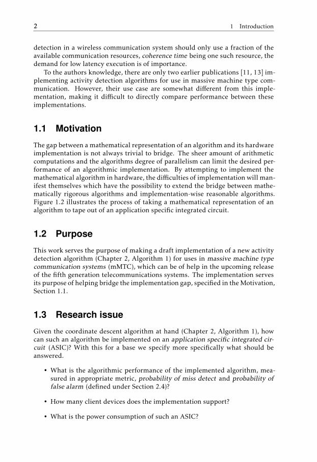
Given the coordinate descent algorithm at hand (Chapter 2, Algorithm 1), howcan such an algorithm be implemented on an application specific integrated cir-cuit (ASIC)? With this for a base we specify more specifically what should beanswered.

• What is the algorithmic performance of the implemented algorithm, mea-sured in appropriate metric, probability of miss detect and probability offalse alarm (defined under Section 2.4)?

• How many client devices does the implementation support?

• What is the power consumption of such an ASIC?

1.4 Delimitations 3

• Is it feasible to implement the algorithm as it is described in Algorithm 1on an ASIC? If not, what could make the algorithm more suitable for imple-mentation without major degradation of performance?

• If the ASIC can not be successfully implemented, what did go wrong? Whatcould/should have been done different in order to succeed?

Mathematicalrepresentation

of algorithm

High levelalgorithm

simulations

Architecturetrue

simulationsHDL code &Synthesis

Circuitsimulation

Tape out

Figure 1.2: Flowchart showing the process of taking an algorithm describedmathematically to one of its corresponding hardware implementation.

1.4 Delimitations

The given scenario, which is described under Section 2.3, requires equipment fortransmitting and receiving wireless data, AD/DA converters and possibly moreequipment in order to operate. The entry point for this solution will be the digi-tal matrix with received signals which is described under Section 2.3. Anythinginvolving the creation of such a matrix, the transfer of signals and conversionbetween digital and analog domain, will not be discussed in this work.

As the focus of this work is on the hardware implementation aspect of thealgorithm, we deliberately leave the work of comparing performance of this ac-tivity detection algorithm to other closely related algorithms and mainly focus onthe degradation of this algorithm throughout the implementation flow. Curiousreaders can find more information and comparisons between activity detectionalgorithms in [3] and [5].

2Theory

This chapter will describe the theory regarding this project. It will briefly startoff by describing the notation and terminology used throughout the work andthe studied mMTC scenario as it is proposed in [5] and [2]. It will also presentthe studied algorithms used for activity detection and introduce the concept ofhardware latency and describe how it can impact implementation size (as in areaon an implemented circuit), power consumption and algorithmic performance.

2.1 Notation

Scalar values are denoted with italic letters (e.g., a or B), vectors are denoted withsmall boldface letters (e.g., c) and matrices are denoted with capital boldfaceletters (e.g., D). The i-th row vector of a matrix D is denoted Di,: and the j-th column vector of the same matrix is denoted D:,j . The Hermitian operationof a complex valued matrix D is denoted DH and such a matrix satisfy DH

i,j =

Dj,i ,∀i, j. The boldface character I is reserved for denoting the identity matrixand its subscript shows the size such that Ik denotes the identity matrix of sizek × k.

Further more, sets are denoted with calligraphic letters (e.g., K) and the car-dinality of a set K is denoted |K| ∈ N. For a scalar V ∈ N we denote the set ofnatural numbers up to V as [V ] = {1, 2, 3, ..., V }.

2.2 Terminology

Before going much further it would be good to summarize and explain some ofthe terms and phrases used throughout this document and to clarify what theauthor means using these terms.

5

6 2 Theory

2.2.1 Performance terms

The term algorithmic performance is used to describe algorithm metrics measur-able standalone from its implementation, i.e, an algorithms statistical probabilityof producing an erroneous result, its rate of convergence or some asymptotic op-eration complexity. These metrics can (in many cases) be thought of as separablefrom the hardware implementation.

The term implementation performance (sometimes system performance orhardware performance) is used to describe performance metrics that is associ-ated with the hardware implementation, i.e, silicon area, power consumption ormaximum system clock frequency.

The author realizes that there is a huge overlap between these two very broadterms, but feels it is of importance to specify these umbrella terms to be able todiscuss the impact of changes made throughout the implementation process.

2.2.2 Hardware terms

Register-transfer level (RTL) is the top abstraction level (least detailed) digitaldescription of a synchronous digital circuit [14]. It is often the description of asynchronous digital system in some hardware description language, i.e, Verilogor VHDL, and the RTL description serves as the last step in this implementation,from which some synthesis tool will generate the necessary objects for fabricatingan application specific integrated circuit (ASIC).

2.2.3 Other terms

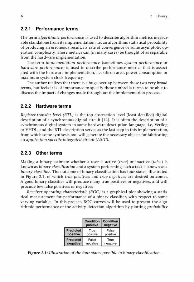
Making a binary estimate whether a user is active (true) or inactive (false) isknown as binary classification and a system performing such a task is known as abinary classifier. The outcome of binary classification has four states, illustratedin Figure 2.1, of which true positives and true negatives are desired outcomes.A good binary classifier will produce many true positives or negatives, and willprocude few false positives or negatives

Receiver operating characteristic (ROC) is a graphical plot showing a statis-tical measurement for performance of a binary classifier, with respect to somevarying variable. In this project, ROC curves will be used to present the algo-rithmic performance of the activity detection algorithm by plotting probability

Truepositive

Truenegative

Falsenegative

Falsepositive

PredictedpositivePredictednegative

Conditionpositive

Conditionnegative

Figure 2.1: Illustration of the four states possible in binary classification.

2.3 Studied scenario 7

of false positives against probability of false negatives (both defined under Sec-tion 2.4) for a varying threshold parameter (presented later in Section 2.5). Foran example of an ROC curve, see the right plot in Figure 3.5.

Whenever a ROC curve is presented throughout the rest of this document, itshows the greatest obtainable performance, that is, the performance when con-vergence has been reached.

2.3 Studied scenario

The scenario studied in this work, is that of a massive MIMO setup with a singlebase station having M antennas. There exist a set Kc of Kc = |Kc | possible usersfrom which the proper subset Ac ⊆ Kc are active users, that is, users in need ofservice from the base station (see Figure 2.2). A block fading channel model [1] isused, i.e., a channel model in which coherence blocks of some adjacent frequencyand time are static (has constant attenuation over frequency and is approximatelytime invariant). Each coherence block consists of Dc signal dimensions. Due tothe requirements put on most wireless communication systems, only a few coher-ence block can be assigned to serve the purpose of activity detection. Further, dueto the sporadic nature of users in this model, the set of active users is consideredsignificantly smaller than the set of possible users Ac = |Ac | � Kc = |Kc |.

The data when transfered over the block fading channel will get slightly dis-torted and some amount of additive white Gaussian noise will be added to the re-ceived signal. The channel for a user k will distort the transferred signal throughthe M-dimensional channel vector hk and add noise z such that the received sig-nal for dimension i ∈ [Dc] will have the form

y[i] =∑k∈Kc

bk√gkak,ihk + z[i] (2.1)

where ak,: denotes the pilot sequence of user k, where gk denotes the transmittedsignal strength, and where bk ∈ {0, 1} is the activity of user k. The channel vectorshk are independent and spatially white i.e., hk ∼ CN (0, IM ).

M antennas

Kc users

inactive

active

Figure 2.2: Illustration of the studied scenario, showing users and the basestation.

8 2 Theory

γ2 = 0.86

γ1 = 0γ0 = 0.93

Figure 2.3: Illustration of the studied scenario, showing users and the basestation.

Further, we describe the entire received signal over all signal dimensions as

Y = AΓ12 H + Z (2.2)

where each column vector of the Dc × Kc matrix A = [a1, ..., aKc ] is the pilotsequence of respective user, where Γ is the Kc × Kc diagonal matrix satisfyingΓk:k = γk ,∀k ∈ [Kc] where in turn γk = bkgk ,∀k ∈ [Kc] is the actual transmittedsignal power for a user k, where H = [h1, ...,hKc ]

T, and where Z is the Dc × Mmatrix satisfying Z:,i = z[i]. We define the average signal to noise ratio (SNR) ofa user k as

SNRk =γkσ2 , k ∈ Ac (2.3)

but leave the motivation for such a definition to [5].

2.4 The problem

The goal of activity detection is to, from the received signal Y and the knownpilot sequences A, find an estimate γ of γ (or Γ of Γ) such that the set of activeusers Ac := {k ∈ Kc : γk > νσ2} can be estimated by Ac := {k ∈ Kc : γk > νσ2} forsome pre-specified threshold ν > 0. An illustration of this shown in Figure 2.3.

Just like in [5] we define the metric probability of miss detection averagedover active users as

pMD (ν) = 1 − E[|Ac(ν) ∩ Ac |]Ac

(2.4)

and the metric probability of false alarm averaged over inactive users as

pFA(ν) =E[|Ac(ν)\Ac |]Kc − Ac

(2.5)

Further, we define a new metric, probability of error, as

pE = minν>0{max{pMD (ν), pFA(ν)}} (2.6)

which will be used to study the convergence with respect to algorithm iterations.

2.5 Algorithm to implement 9

2.5 Algorithm to implement

Coordinate descent is an algorithm used for finding the minimum (or maximum)point in smooth convex functions. By making an initial guess at a set of coorid-nates, the algorithm optimizes and moves the current estimate along one coor-dinate at a time, for each iteration, until convergence is reached (a minimum isfound) or for a fixed number of iterations. In this work, coordinate descent isused to minimize a likelihood statistic estimate of γ as described in [5].

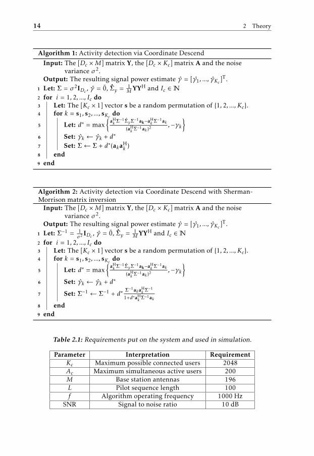
The primary algorithm of coordinate descent for activity detection with max-imum likelihood estimator was first described in [5] and can be seen in Algo-rithm 1. A slightly modified version with Sherman-Morrison matrix inversion [12]is described in [2] which utilizes matrix inverse updating during operation to sur-pass the need of explicitly evaluating matrix inverses for each iteration (Line 7in Algorithm 2). Note that the Sherman-Morrison matrix inversion is not anestimate of a matrix inversion, but a derive mathematical theorem, making theoutput estimate γ of Algorithm 1 and Algorithm 2 exactly equivalent.

Notice that, on Line 3 in Algorithms 1 and 2, coordiantes are selected at ran-dom. It is proven that selecting coordinates randomly give the algorithm a muchgreater convergence rate than updating coordinates in a static fashion, and it istherefor a common approach when constructing coordinate descent algorithms[4].

In Algorithms 1 and 2, input σ2 should ideally be chosen (and is in this workchosen) according to

σ2 =γ

SNR(2.7)

where γ = γk ,∀k ∈ Ac and SNR = SNRk ,∀k ∈ Ac. Further, Ic ∈ N denotes thedesired number of iterations to perform in the algorithm.

2.5.1 Updating the variance estimate

As can be seen, the only difference between Algorithms 1 and 2 is the usage ofthe Sherman-Morrison matrix inversion[12] (Algorithm 2, Line 7) to update theinverse of a variance estimate component Σ. This approach of updating the in-verse makes sense from an implementation point of view since only the inverseof Σ is used in the algorithm. It is used as an intermediate value only to calculatethe real algorithm output. Even more importantly, from an implementation per-spective the explicit inverse of a full matrix is both computationally expensiveand comes with a lot of latency, possibly slowing down an implementation.

2.5.2 Performance requirements

Requirements on the implementation performance are used to steer developmentin a direction that will make the implementation as useful as possible. The re-quirements used for this project is a fusion of requirements used in previousworks ([5], [2]) aswell as feedback given from Prof. Erik G. Larsson from the Di-vision of Comunication Systems in the Department of Electrical Engeneering atLinköping University. The requirements on the system are displayed in Table 2.1.

10 2 Theory

Note especially that the parameter Ac is the number of active users at anygiven time, i.e., all users can be active as long as no more than Ac users are ac-tive simultainously. With the Internet of Things being one of the main focus in5G-MIMO technology, it makes sense to assume that only a fraction of all pos-sible users are active at any given moment. The algorithm operating frequencyf is chosen such that the demand for low latency, which comes with 5G, can besatisfied.

2.6 Hardware aspects of implementation

This section will describe some theory behind the implementation. When takingan algorithm from its mathematical representation to one of its hardware imple-mentation there are many things to consider such as numeric representations,word lengths, timings and much more.

2.6.1 Numeric representation

In every hardware implementation, each arithmetic operation and intermediatedata storage is performed with some numeric representation suitable for the al-gorithm in question. We select such representations based on the dynamic rangeand numerical precision required for application performance and functionality.

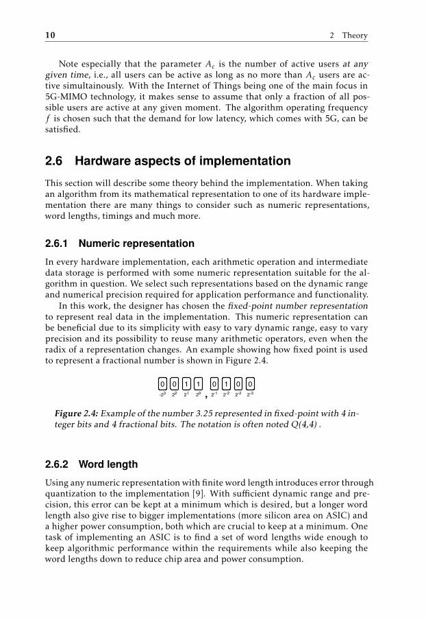
In this work, the designer has chosen the fixed-point number representationto represent real data in the implementation. This numeric representation canbe beneficial due to its simplicity with easy to vary dynamic range, easy to varyprecision and its possibility to reuse many arithmetic operators, even when theradix of a representation changes. An example showing how fixed point is usedto represent a fractional number is shown in Figure 2.4.

0 0 1 1 0 1 0 0,202122-23 2-1 2-2 2-2 2-3

Figure 2.4: Example of the number 3.25 represented in fixed-point with 4 in-teger bits and 4 fractional bits. The notation is often noted Q(4,4) .

2.6.2 Word length

Using any numeric representation with finite word length introduces error throughquantization to the implementation [9]. With sufficient dynamic range and pre-cision, this error can be kept at a minimum which is desired, but a longer wordlength also give rise to bigger implementations (more silicon area on ASIC) anda higher power consumption, both which are crucial to keep at a minimum. Onetask of implementing an ASIC is to find a set of word lengths wide enough tokeep algorithmic performance within the requirements while also keeping theword lengths down to reduce chip area and power consumption.

2.6 Hardware aspects of implementation 11

In this work, a word length sweep of each internal node will be conductedto evaluate algorithmic performance vs word length. It is desirable to keep theperformance roughly within the double-precision floating-point simulated per-formance.

2.6.3 Combinational latency

An application specific integrated circuit is, as the name suggests, an electricaldevice with some specific purpose implemented on an integrated circuit, usuallyin some CMOS process (in this case a 28-nm FD-SOI CMOS process). Parasiticelectrical phenomenons, such as parasitic capasitance and inductance, will limitthe propagation speed of electrical signals within the circuit. The time it takesfor an electrical signal to propagate from one node in the system to another node(time taken between stimulation and response) is called latency. The time it takesfor an electrical signal to propagate from one flip-flop to another, through somecombinational logic, is called combinational latency.

2.6.4 Critical path

When making high performance circuits, the concept of latency is uttermost cru-cial to take into consideration when designing, since the greatest combinationallatency in the system, the critical path, will limit the maximum clock frequencyunder which the implementation will function properly, and therefore put a limiton how fast the implementation can operate. The maximum combinational la-tency of the system Tmax will limit the maximum operating clock frequency fmaxaccording to

fmax =1

Tmax(2.8)

and an operating frequency greater than this theoretical maximum frequencywill break intended synchronous behavior by using the result in a node before itis ready.

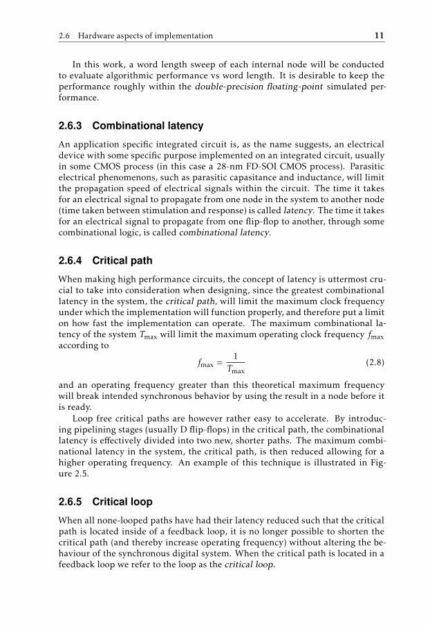
Loop free critical paths are however rather easy to accelerate. By introduc-ing pipelining stages (usually D flip-flops) in the critical path, the combinationallatency is effectively divided into two new, shorter paths. The maximum combi-national latency in the system, the critical path, is then reduced allowing for ahigher operating frequency. An example of this technique is illustrated in Fig-ure 2.5.

2.6.5 Critical loop

When all none-looped paths have had their latency reduced such that the criticalpath is located inside of a feedback loop, it is no longer possible to shorten thecritical path (and thereby increase operating frequency) without altering the be-haviour of the synchronous digital system. When the critical path is located in afeedback loop we refer to the loop as the critical loop.

12 2 Theory

C1 C2D QD QIn Out

clk

Figure 2.5: Example of a non-looped path in which the critical path couldbe reduced by introducing a D flip-flop between combinatorial networks C1and C2.

C1 C2D QD QIn

Out

clk

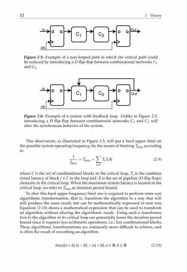
Figure 2.6: Example of a system with feedback loop. Unlike in Figure 2.5,introducing a D flip-flop between combinatorial networks C1 and C2 willalter the synchronous behavior of the system.

This observation, as illustrated in Figure 2.5, will put a hard upper limit onthe possible system operating frequency, by the means of limiting Tmax accordingto

1fmax

= Tmax =∑i∈C

Ti / |A| (2.9)

where C is the set of combinational blocks in the critical loop, Ti is the combina-tional latency of block i ∈ C in the loop and A is the set of pipeline (D flip-flops)elements in the critical loop. When the maximum system latency is located in thecritical loop, we refer to Tmax as iteration period bound.

To alter this hard upper frequency limit one is required to perform some sortalgorithmic transformation, that is, transform the algorithm in a way that willstill produce the same result, but can be mathematically expressed in new way.Equation (2.10) shows a mathematical expression that can be used to transforman algorithm without altering the algorithmic result. Using such a transforma-tion to the algorithm in its critical loop can potentially lower the iteration periodbound since it requires less arithmetic operations, i.e., less combinational blocks.These algorithmic transformations are commonly more difficult to achieve, andis often the result of reworking an algorithm.

max{|a + b|, |a − b|} = |a| + |b|, a ∈ R, b ∈ R (2.10)

2.6 Hardware aspects of implementation 13

2.6.6 Isomorphic implementation

An isomorphic implementation (also known as injective implementation or 1-to-1 mapping) is a way of implementing an algorithm in which each operation inthe algorithm is mapped to an individual process element such that there existsa 1-to-1 mapping between each algorithm operation and each process element.Figure 2.7 tries to illustrate this concept. What makes an isomorphic implemen-tation interesting is the observation that, for any given algorithm (that wouldnot undergo any algorithm transformation), the isomorphic implementation willhave the least amount of operational overhead and thereby be the fastest imple-mentation. It is usually also the implementation with lowest power consumptionper performance, but the isomorphic implementations usually consumes hugearea compared to an implementation that reuses process elements for differentalgorithm operations, and will therefore be very expansive to fabricate.

Due to the fact that no previous implementation of this algorithm were foundduring the research phase of this project, and due to the difficulties in estimatingthe iteration period bound of an implementation of Algorithm 2, it makes senseto make a first attempt at an isomorphic implementation of the algorithm to seeif it will be possible to make an implementation that will meet the throughput/la-tency performance requirements without undergoing any algorithm transforma-tions. It was clear very early that the iteration period bound of the algorithm willbe large (see flow graph, Figure 3.8) and it is therefore uncertain if it is possibleto satisfy the requirements on latency and throughput of the system.

PE1 D PE2 D PE3In Out Control &

Memory PEx

Control signals

InOut

a) b)

Figure 2.7: Example illustrating two implementations of the some same al-gorithm as a) isomorphic implementation where there exists one process el-ement for evaluating each algorithm step and b) polymorphic implementa-tion where a programmable process element is reused for the three differentstages and controlled through some control unit.

14 2 Theory

Algorithm 1: Activity detection via Coordinate Descend

Input: The [Dc ×M] matrix Y, the [Dc × Kc] matrix A and the noisevariance σ2.

Output: The resulting signal power estimate γ = [γ1, ..., γKc ]T.

1 Let: Σ = σ2IDc , γ = 0, Σy = 1MYYH and Ic ∈ N

2 for i = 1, 2, ..., Ic do3 Let: The [Kc × 1] vector s be a random permutation of {1, 2, ..., Kc}.4 for k = s1, s2, ..., sKc do

5 Let: d∗ = max{

aHk Σ−1ΣyΣ−1ak−aH

k Σ−1ak

(aHk Σ−1ak )2 ,−γk

}6 Set: γk ← γk + d∗

7 Set: Σ← Σ + d∗(akaHk )

8 end9 end

Algorithm 2: Activity detection via Coordinate Descend with Sherman-Morrison matrix inversion



1 Let: Σ−1 = 1σ2 IDc , γ = 0, Σy = 1

MYYH and Ic ∈ N2 for i = 1, 2, ..., Ic do3 Let: The [Kc × 1] vector s be a random permutation of {1, 2, ..., Kc}.4 for k = s1, s2, ..., sKc do

5 Let: d∗ = max{


k Σ−1ak



7 Set: Σ−1 ← Σ−1 + d∗Σ−1akaH

k Σ−1

1+d∗aHk Σ−1ak

8 end9 end

Table 2.1: Requirements put on the system and used in simulation.

Parameter Interpretation RequirementKc Maximum possible connected users 2048Ac Maximum simultaneous active users 200M Base station antennas 196L Pilot sequence length 100f Algorithm operating frequency 1000 Hz

SNR Signal to noise ratio 10 dB

3Results of isomorphic

implementation

This chapter will present the results and findings of the isomorphic implementa-tion of Algorithm 2. It will start of by describing the four different models thatwere created and used to verify the behaviour of the system. After that, the chap-ter will present some techniques used to reduce the resulting silicon area andpossibly increase the operating frequency.

3.1 Models

To generate a final working and somewhat modular implementation, which shouldbe easy to verify, models of increasing detail were generated until a final RTLmodel could be produced. For each new model of increasing deatil, the previ-ous model was used as a reference model for verifying the behavior of the newsystem.

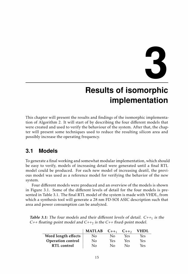
Four different models were produced and an overview of the models is shownin Figure 3.1. Some of the different levels of detail for the four models is pre-sented in Table 3.1. The final RTL model of the system is made with VHDL, fromwhich a synthesis tool will generate a 28 nm FD-SOI ASIC description such thatarea and power consumption can be analyzed.

Table 3.1: The four models and their different levels of detail. C++1 is theC++ floating-point model and C++2 is the C++ fixed-point model.

MATLAB C++1 C++2 VHDLWord length effects No No Yes YesOperation control No Yes Yes Yes

RTL control No No No Yes

15

16 3 Results of isomorphic implementation

MATLABModel

C++ modelusing

floating-pointarithmetic

C++ modelusing

fixed-pointarithmetic

RTLVHDL model

More detailLess detail

Figure 3.1: Overview of the four different models used throughout theproject.

3.1.1 MATLAB model

An initial MATLAB high level simulation model had previously been made bythe Division of Communication Systems to asses the algorithms statistical proper-ties compared to some other activity detection algorithms. This MATLAB modelserved as the starting point for this implementation and was used extensively fortesting modifications of the model to ease the work later in the more detailedmodels. The code for this model is attached to Appendix B.

It was also in the MATLAB model that the first word length simulations wereadded. Even tough the underlying numeric data type used in MATLAB to repre-sent real numbers is the IEEE 754 binary64 type (commonly known an double-precision floating-point ), it was possible to introduce some finite word lengtheffects trough the use of emulated fixed point. Emulating the use of fixed-pointnumber helped get a first glance of what word lengths to use in the later moredetailed models. The fixed point emulation is shown in Figure 3.2.

However, since all matrix operations performed in the MATLAB model arestill evaluated using double-precision floating-point arithmetic, the result willdiffer from that of an implementation were all operations, including the internalmatrix/vector sub-operations, are performed entirely with fixed point numbers.Therefore, this model can not be used for verifying the later RTL-VHDL model ofthe implementation, but it is useful in that it is easy to modify and its results canbe used as reference for other models.

double x

int ndouble out

Figure 3.2: Fixed point emulation block used in the MATLAB model. Theblock will evaluate the double-precision floating-point number closest to in-put x represented as a fixed-point number with n fractional bits.

3.1 Models 17

+

+

a

b

d

c

c

d

Re

Im

a) (a+bi)(c+di)

+

+

b

a

d

c

c

d

Im

Re

b) (a+bi)(c-di)

+

+

a

b

c

d

d

c

Im

Re

c) (a-bi)(c+di)

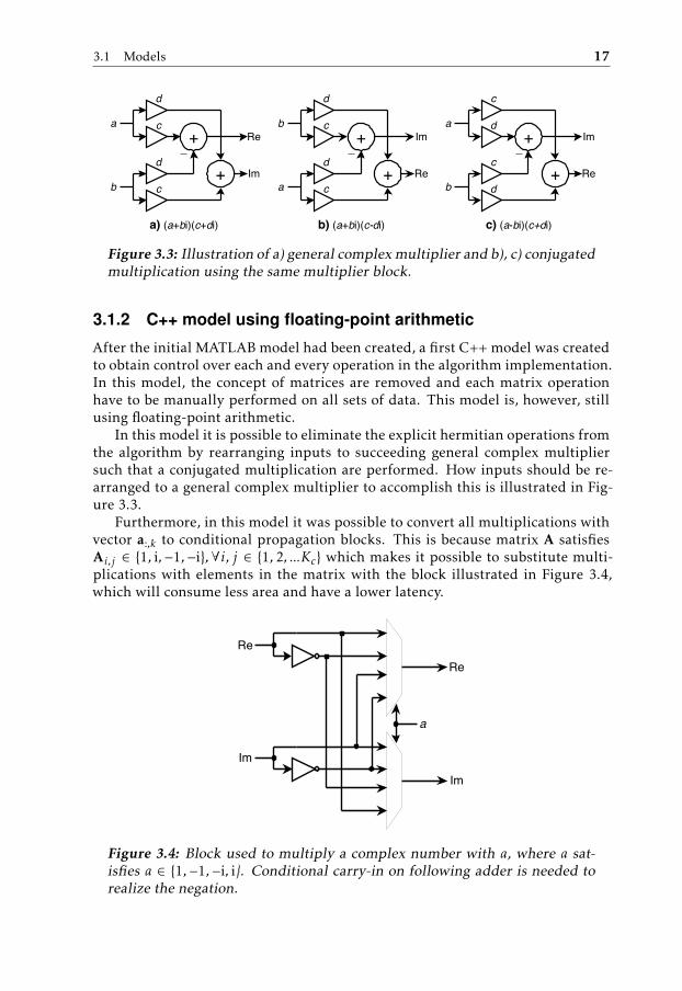
Figure 3.3: Illustration of a) general complex multiplier and b), c) conjugatedmultiplication using the same multiplier block.

3.1.2 C++ model using floating-point arithmetic

After the initial MATLAB model had been created, a first C++ model was createdto obtain control over each and every operation in the algorithm implementation.In this model, the concept of matrices are removed and each matrix operationhave to be manually performed on all sets of data. This model is, however, stillusing floating-point arithmetic.

In this model it is possible to eliminate the explicit hermitian operations fromthe algorithm by rearranging inputs to succeeding general complex multipliersuch that a conjugated multiplication are performed. How inputs should be re-arranged to a general complex multiplier to accomplish this is illustrated in Fig-ure 3.3.

Furthermore, in this model it was possible to convert all multiplications withvector a:,k to conditional propagation blocks. This is because matrix A satisfiesAi,j ∈ {1, i,−1,−i},∀i, j ∈ {1, 2, ...Kc} which makes it possible to substitute multi-plications with elements in the matrix with the block illustrated in Figure 3.4,which will consume less area and have a lower latency.

Re

Im

Re

Im

a

Figure 3.4: Block used to multiply a complex number with a, where a sat-isfies a ∈ {1,−1,−i, i}. Conditional carry-in on following adder is needed torealize the negation.


3.1.3 C++ model using fixed-point arithmetic

The second C++ model was based on the first C++ model but the underlyingnumeric data type was changed from floating-point numbers to fixed-point. ThisC++ model can be tested against previous reference models to verify algorithmicperformance and then be used to verify the final RTL-VHDL model.

It was in this model that the choices for word lengths of each operation wasfinalized. This model served as the link between the difficult to modify RLTmodel and the very modular initial models.

3.1.4 RTL VHDL model

After the three earlier models had been created, it was rather straight forwardto create the VHDL model. The goal when making this model was to make itdo exactly what the previous model, the C++ model using fixed point arithmetic,was doing such that the VHDL model could be verified against it. This modelwill also be synthesizable making it possible to generate an ASIC.

Due to the complexity of making high level optimizations to the algorithmwith this model, no new optimizations were introduced in this model. The verifi-cation of this model is described under Section 3.4.

3.2 Sequence

The algorithm as it is described in [2] and [5] propose updating users estimatedchannel strength at random, one time per coordinate descent iteration (Algo-rithm 2, Line 3). With the given communication model described under Sec-tion 2.3 and the requirements outlined in Table 2.1, the resulting algorithmicperformance of the algorithm is shown in Figure 3.5.

With this method of selecting users at random within each coordinate descentiteration, one can see that the maximum algorithmic performance is reachedwithin five, or no more than six coordinate descent iterations (left plot, Figure 3.5).For the sake of implementation we would like to avoid implementing an ad-vanced random number permutator into the implementation. It is desirable tofind a way of selecting users according to some scheme such that the algorithmconvergence is still like, or close to, that of the fully randomized user sequencepresented in Figure 3.5. A user selection scheme whose convergence is not fastenough will force the implementation to evaluate more coordinate descent iter-ations to attain the same algorithmic performance which will result in a slowerand bigger implementation.

3.2.1 Random sequences with memories

At first, the idea of pre-generating some random sequence and than reusing thosesequences between iterations or between algorithm runs were tested. This, how-ever, is undesirable in that it requires memories to store the random sequencesfor usage. The result is presented in Figure 3.6.

3.2 Sequence 19

1 2 3 4 5 6 7

Iterations

10-6

10-5

10-4

10-3

10-2

10-1

100

Pro

babili

ty o

f E

rror

Iteration vs Error

Random sequence

10-6

10-5

10-4

10-3

Probability of Miss Detection

10-6

10-5

10-4

10-3

Pro

babili

ty o

f F

als

e A

larm

ROC

Random sequence

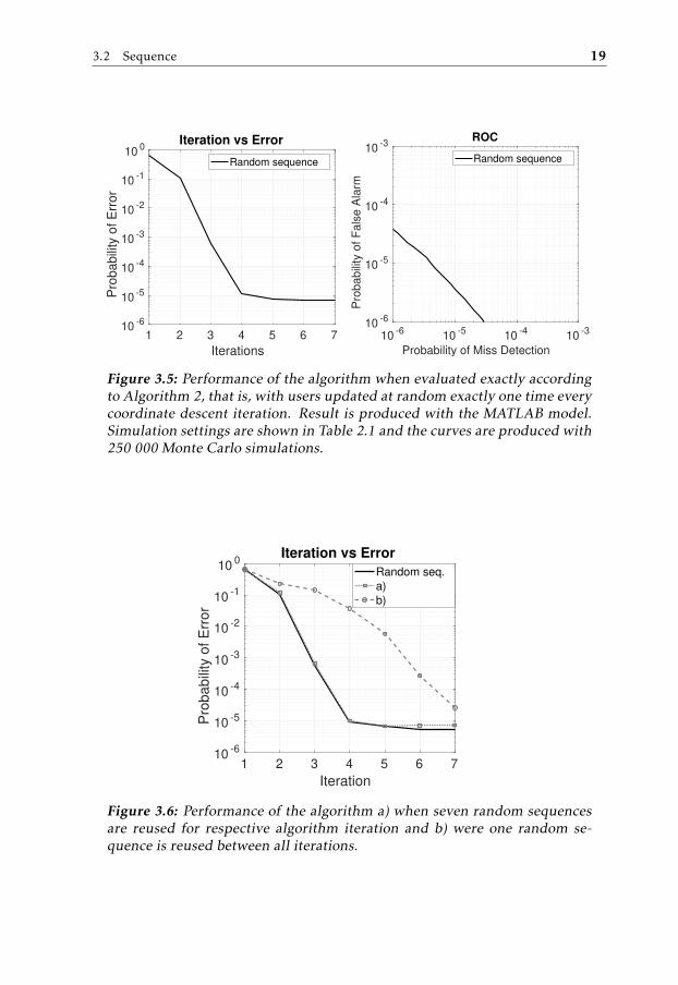
Figure 3.5: Performance of the algorithm when evaluated exactly accordingto Algorithm 2, that is, with users updated at random exactly one time everycoordinate descent iteration. Result is produced with the MATLAB model.Simulation settings are shown in Table 2.1 and the curves are produced with250 000 Monte Carlo simulations.

1 2 3 4 5 6 7

Iteration

10-6

10-5

10-4

10-3

10-2

10-1

100

Pro

ba

bili

ty o

f E

rro

r

Iteration vs Error

Random seq.

a)

b)

Figure 3.6: Performance of the algorithm a) when seven random sequencesare reused for respective algorithm iteration and b) were one random se-quence is reused between all iterations.


The strategy of pre-generating six or seven random sequences and reusingthese sequences shows promising results [a) in Figure 3.6] , however, since thismethod of selecting users will require memories to store the sequences, it is betterto try find a sequence that can be generated at runtime, that will not have toutilize memories (or advanced random number permutators).

It is worth mentioning that reusing one random sequence between all algo-rithm iterations [b) in Figure 3.6] converges as slow as updating users accordingto the sequence {1, 2, 3, ..., Kc} in all iterations. This seems to indicates that, forgood convergence, it is more important to have sequences that vary greatly be-tween iteration than it is to have randomness within each iteration.

3.2.2 Pseudo random modulo sequence

A pseudo random permutation that can be generated on the fly, without memo-ries, that makes the algorithm reach its minimum probability of error within fiveor six iteration, is desirable. Equation

ki,j = (2i + 1)j mod Kc, i ∈ {0, ..., Ic − 1}, j ∈ {0, ..., Kc − 1} (3.1)

can be used to generate permutations of the set {0, 1, 2, ..., Kc − 1}. In (3.1), Ic isused to denote the desirable number of coordinate descent iterations to performand Kc the maximum number of possible users in the system.

Selecting users according to this equation will, from an implementation per-spective, be a good choice. It requires two counters, one for counting coordinatedescent iteration and one for counting users within an interation, plus some sim-ple arithmetic, an adder plus two multipliers. If choosing Kc as a power of two(as in the requirements, Table 2.1) the modulo operation can be performed byusing the log2(Kc) least significant bits in the result of (2i + 1)j.

The matrix

k0,0 k0,1 k0,2 . . . k0,Kc−1k1,0 k1,1 k1,2 . . . k1,Kc−1k2,0 k2,1 k2,2 . . . k2,Kc−1...

......

. . ....

kIc ,0 kIc ,1 kIc ,2 . . . kIc−1,Kc−1

=

0 1 2 . . . Kc − 10 3 6 . . . Kc − 30 5 10 . . . Kc − 5...

......

. . ....

0Ic 1Ic 2Ic . . . Kc − 2Ic − 1

(3.2)

visualizes how users are selected according to this scheme. Note that, in eachnew coordinate descent iteration, every user is selected exactly once. Each rowin (3.2) represents one iteration of coordinate descent and each column representone user.

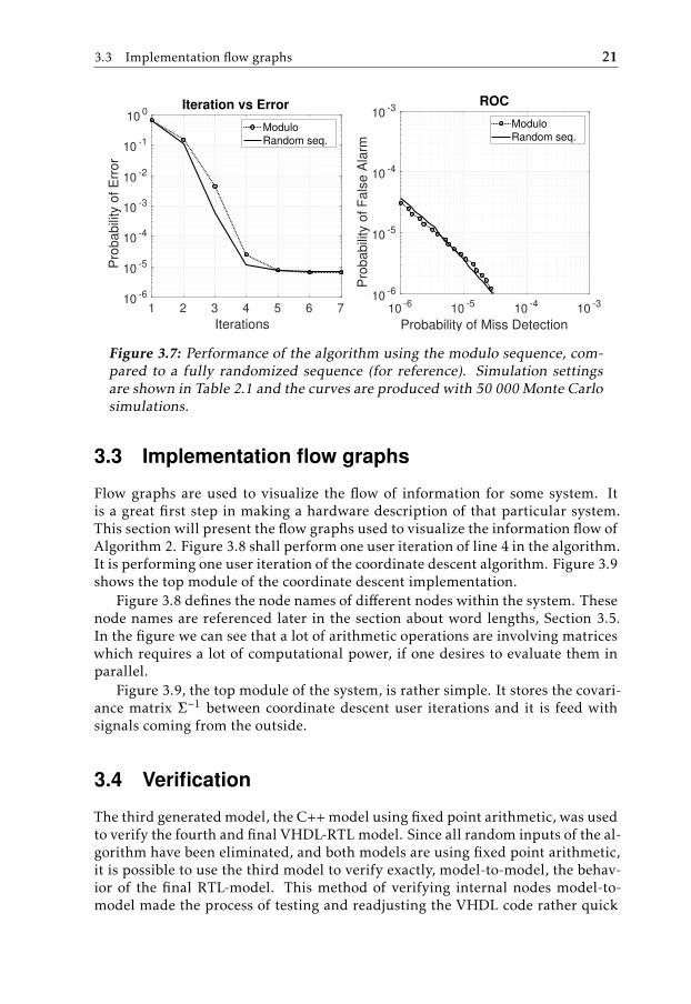
The resulting performance of using this strategy is shown in Figure 3.7. In itwe can see that the convergence of the algorithm is a somewhat slower for the firstfew iterations than compared to the algorithm using fully random user selection.However it can be seen that the modulo random strategy still reaches the maxi-mum performance (minimum probability of error) for five to six iteration. Sincethe goal is to reach best possible performance, it does not matter that it convergesa little slower for the first few iterations, as long as the maximum performance isreached around the same iteration.

3.3 Implementation flow graphs 21

1 2 3 4 5 6 7

Iterations

10-6

10-5

10-4

10-3

10-2

10-1

100

Pro

babili

ty o

f E

rror

Iteration vs Error

Modulo

Random seq.

10-6

10-5

10-4

10-3


10-6

10-5

10-4

10-3

Pro

babili

ty o

f F

als

e A

larm

ROC

Modulo

Random seq.

Figure 3.7: Performance of the algorithm using the modulo sequence, com-pared to a fully randomized sequence (for reference). Simulation settingsare shown in Table 2.1 and the curves are produced with 50 000 Monte Carlosimulations.

3.3 Implementation flow graphs

Flow graphs are used to visualize the flow of information for some system. Itis a great first step in making a hardware description of that particular system.This section will present the flow graphs used to visualize the information flow ofAlgorithm 2. Figure 3.8 shall perform one user iteration of line 4 in the algorithm.It is performing one user iteration of the coordinate descent algorithm. Figure 3.9shows the top module of the coordinate descent implementation.

Figure 3.8 defines the node names of different nodes within the system. Thesenode names are referenced later in the section about word lengths, Section 3.5.In the figure we can see that a lot of arithmetic operations are involving matriceswhich requires a lot of computational power, if one desires to evaluate them inparallel.

Figure 3.9, the top module of the system, is rather simple. It stores the covari-ance matrix Σ−1 between coordinate descent user iterations and it is feed withsignals coming from the outside.

3.4 Verification

The third generated model, the C++ model using fixed point arithmetic, was usedto verify the fourth and final VHDL-RTL model. Since all random inputs of the al-gorithm have been eliminated, and both models are using fixed point arithmetic,it is possible to use the third model to verify exactly, model-to-model, the behav-ior of the final RTL-model. This method of verifying internal nodes model-to-model made the process of testing and readjusting the VHDL code rather quick


Σ-1*

AHS2

Σy *

S1

*

*

+N1

N2

-

X2

A[:,k]

MAX

L x 1

L x

1+ 1

1 x

Lδ

+*

L x L

L x 1

L x L

L x L

N3

+

γ[k]

γ[k]

Σ-1L x L

L x L

Σ-1L x L

N4

*

Q

- γ[k]

*

Figure 3.8: Flow graph of the coordinate descent block. Asterisks (*) denoteleft hand side of operator when appropriate. [a × b] denote a matrix of ’a’rows and ’b’ columns. Names on the arcs (e.g, S2) are used to name nodes.

CDA[:,k]

L x 1

γ[k]

D

Σy

L x

L

Σ-1

L x

L

γ[k]

Σ-1 L x

L

Figure 3.9: Flow graph of the coordinate descent top module. CD is a blockof the flow graph in Figure 3.8.

3.5 Word length simulations 23

MATLABStimuli generation

C++/MexReference model Se

d/AW

Kfil

ter

Pythonto_binary

VHDL Testbench

Coordinate Descent VHDL model

Pythonto_decimal

Diffcomparison

Reference Testee

result

Mod

elSi

m S

imul

ator

Figure 3.10: Figure showing method of verifying the RTL-VHDL modelagainst the C++ model.

and easy. The C++ fixed-point and VHDL model-to-model verification setup isillustrated in Figure 3.10.

The verification system uses MATLAB to generate stimuli data for the C++model, and the output of the C++ model is used as a reference for the VHDLmodel. The MATLAB stimuli data is also filtered through some standard Unixtools and converted to binary with Python. The binary stimuli data is feed to aVHDL test bench, and the test bench is simulated with the ModelSim Simulator.The test bench output is converted back to decimal with python and compared tothe C++ reference output (both actual algorithm output and intermediate nodevalues are compared) through another standard unix tool. Running a couple ofsimulations showed that the node values of all internal nodes of the C++ fixedpoint model and the VHDL model matched exactly.

3.5 Word length simulations

A set of word length simulations was conducted in an attempt to optimize wordlengths for retaining the maximum algorithmic performance while minimizingthe word lengths (more under Section 2.6.2). The data in each node is quantizedto be represented by some number of fixed point binary and these were in turnsweept.

3.5.1 Integer bits

By extracting and visualizing node values when data flows through the system, itis possible to run simulations and than extract the maximum value for each node.This maximum value for some node, amax ∈ R, can be used to get a quantitativemeasurement of the required integer bits, nint, for the implementation according


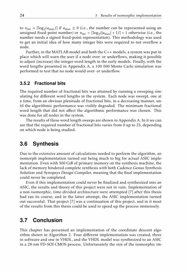
to nint = dlog2(amax)e if amax ≥ 0 (i.e., the number can be represented using anunsigned fixed-point number) or nint = dlog2(|amax| + 1)e + 1 otherwise (i.e., thenumber needs a signed fixed-point representation). This methodology was usedto get an initial idea of how many integer bits were required to not overflow anode.

Further, in the MATLAB model and both the C++ models, a system was put inplace which will warn the user if a node over- or underflows, making it possibleto adjust (increase) the integer word length in the early models. Finally, with theword lengths presented in Appendix A, a 100 000 Monte Carlo simulation wasperformed to test that no node would over- or underflow.

3.5.2 Fractional bits

The required number of fractional bits was attained by running a sweeping sim-ulating for different word lengths in the system. Each node was sweept, one ata time, from an obvious plenitude of fractional bits, in a decreasing manner, un-til the algorithmic performance was visibly degraded. The minimum fractionalword length that did not affect the algorithmic performance was chosen. Thiswas done for all nodes in the system.

The results of these word length sweeps are shown in Appendix A. In it we cansee that the required number of fractional bits varies from 0 up to 25, dependingon which node is being studied.

3.6 Synthesis

Due to the extensive amount of calculations needed to perform the algorithm, anisomorph implementation turned out being much to big for actual ASIC imple-mentation. Even with 500 GiB of primary memory on the synthesis machine, thelack of memory hindered complete synthesis with both Cadence Genus SynthesisSolution and Synopsys Design Compiler, meaning that the final implementationcould never be completed.

Even if this implementation could never be finalized and synthesized into anASIC, the results and theory of this project were not in vain. Implementation ofa non-isomorphic, time-divided architecture were attempted [7] after this thesishad ran its course, and in the latter attempt, the ASIC implementation turnedout successful. That project [7] was a continuation of this project, and in it mostof the results from this thesis could be used to speed up the process immensely.

3.7 Conclusion

This chapter has presented an implementation of the coordinate descent algo-rithm shown in Algorithm 2. Four different implementation was created, threein software and one in VHDL, and the VHDL model was synthesized to an ASICin a 28-nm FD-SOI CMOS process. Unfortunately the size of the isomorphic im-

3.7 Conclusion 25

plementation hindered this implementation from succeeding, but a time-dividedarchitecture was attempted [7] in which generating the ASIC proved successful.

4Investigation of parallel algorithm

This chapter will present some further findings of the project which can be of in-terest if acceleration of algorithm operation frequency is desirable. It will presenta parallelizable version of the coordinate descent algorithm and we will throughsimulation motivate an almost non-existing degradation of algorithmic perfor-mance using the parallel algorithm.

Further, this chapter will show that the more general Woodbury matrix iden-tity, as opposed to the Sherman-Morrison matrix inversion, can be used to reducethe size of the otherwise [L×L] large matrix inversion, even in the parallel versionof the algorithm.

4.1 Parallel execution

A first impression of Algorithms 1 and 2 is that both algorithms are rather se-quential in that they perform one Coordinate Descent update stage (Algorithm 1,Line 5-6) for some possible user k and then update the variance estimate compo-nent, Σ or Σ−1, before proceeding doing the same operation again for a new userk, only this time with a new estimate of the variance component. This sequen-tial outline of the algorithm puts a tight limit on the speed we can achieve onan implementation of the algorithm. Therefore it makes sense to explore a moreparallel version of the algorithm, one that does not lose us any algorithmic per-formance while doing so. In [10] it is argued that “... coordinate descent methodscan be accelerated by parallelization when applied to the problem of minimizingthe sum of a partially separable smooth convex function and a simple separableconvex function.” When applying such a technique to Algorithm 1 we get a vari-ant in which the Coordinate Descent update stages can be performed in parallelto significantly increase the achievable speed of the algorithm. Through simu-lations we will motivate the non degradation of the algorithm for usage against

27

28 4 Investigation of parallel algorithm

the non parallelized counterpart. The parallelized algorithm is described in Al-gorithm 3.

Algorithm 3: Activity detection via Parallel Coordinate Descend



1 Let: Σ = σ2IDc , γ = 0, Σy = 1MYYH, Ic ∈ N and P = degree of parallelism.

2 for i = 1, 2, ..., Ic do3 Let: The [Kc × 1] vector s be a random permutation of {1, 2, ..., Kc}.4 for j = 1, 2, ..., KcP do5 parallel for k = s1+jP , s2+jP , ..., sKc/P+jP do

6 Let: d∗k = max{


k Σ−1ak



8 end

9 Set: Σ← Σ +∑k

d∗k(akaHk )

10 end11 end

A MATLAB high level model of the parallel coordinate descent algorithm wascreated and simulated. Simulations were performed with settings as describedin Table 2.1, and the results can be seen in Figure 4.1. A quick reminder that Pdenotes the level of parallelism for the algorithm. In Figure 4.1 we can clearly seethat the performance degradation is non existing for degrees of parallelism up to256 out of 2048. For 512 users out of 2048 evaluated in parallel it can be seen thatthe algorithm breaks down. If given infinite silicon area for the implementation,the degree of parallelism P could potentially result in roughly a P times as fastimplementation, since most of the latency resulted from the algorithm comesfrom this inner loop (Algorithm 3, Line 5).

4.2 Reducing the size of matrix inverse in parallelcoordinate descent

The primary difference between Algorithm 1 and 2 can be found in Line 7 werethe authors of [2] suggest updating the covariance component inverse (Σ−1) in-stead of the covariance component (Σ) through the use of Sheerman-Morrisonsformula [12]. Computationally, this transforms an explicit [L × L] matrix inverseto some basic matrix arithmetic. Sheerman-Morrisons formula is shown in Equa-tion 4.1 (

Σ + akd∗kaHk

)−1= Σ−1 − d∗k

Σ−1akaHk Σ−1

1 + d∗kaHk Σ−1ak

(4.1)

4.2 Reducing the size of matrix inverse in parallel coordinate descent 29

1 2 3 4 5 6 7

Iterations

10-6

10-5

10-4

10-3

10-2

10-1

100

Pro

babili

ty o

f E

rror

Iteration vs Error

P = 32

P = 64

P = 128

P = 256

P = 512

Sequential

10-6

10-5

10-4

10-3


10-6

10-5

10-4

10-3

Pro

ba

bili

ty o

f F

als

e A

larm

ROC

P = 32

P = 64

P = 128

P = 256

P = 512

Sequential

Figure 4.1: Performance of the parallel coordinate descent algorithm forsome different level of parallelism.

However, for the parallel version of coordinate descent it is necessary to updateΣ−1 according to

Σ−1 ←

Σ +P∑p=1

apd∗paHp

−1

(4.2)

where P is the number of parallel users in coordinate descent to update in par-allel. To evaluate the right hand side of (4.2) (without explicitly performing theinverse), one need turn to the more general Woodbury matrix identity [6] (fromwhich Sherman-Morrison formula can be derived). Woodburys matrix identity,when using this works notation, can be expressed as(

Σ + A:,[k:k+p]DAH:,[k:k+p]

)−1=

Σ−1 − Σ−1A:,[k:k+p]

(D−1 + AH

:,[k:k+p]Σ−1A:,[k:k+p]

)−1AH

:,[k:k+p]Σ−1

(4.3)

where A:,[k:k+p] =[ak ak+1 ... ak+p

]is the [L × p] matrix of pilot sequences for

users {k, k + 1, k + p} ⊆ Kc and where D = diag{d∗k , d∗k+1, ..., d

∗k+p} ⇐⇒ D−1 =

diag{ 1d∗k, 1d∗k+1

, ..., 1d∗k+p}. With the following example

(Σ + a1d∗1aH1 + a2d

∗2aH2 + a3d

∗3aH3 )−1 =

(Σ + A:,[1:3]DAH

:,[1:3]

)−1(4.4)

we can see how the identity can be used to evaluate the update of covariancematrix Σ−1 from three users being evaluated in parallel.

At first glance the result in (4.3) seems to bring more work than simplifica-tion. However, note that quite a bit of partial results in the right hand side havealready previously been evaluated and can simply be reused. More specifically,all elements in the matrix product

Σ−1A:,[k:k+p] =[Σ−1ak Σ−1ak+1 ... Σ−1ak+p

](4.5)


have already been evaluated previously in the algorithm, moreover, all elementsin the matrix product

AH:[k:k+p]Σ

−1 =[aHk Σ

−1 aHk+1Σ−1 ... aHk+pΣ

−1]T

(4.6)

have also previously been evaluated in the algorithm and furthermore the diago-nal elements of matrix product

AH:,[k:k+p]Σ

−1A:,[k:k+p] =

aHk Σ

−1ak aHk Σ−1ak+1 . . . aHk Σ

−1ak+paHk+1Σ

−1ak aHk+1Σ−1ak+1 . . . aHk+1Σ

−1ak+p...

.... . .

...aHk+pΣ

−1ak aHk+pΣ−1ak+1 . . . aHk+pΣ

−1ak+p

(4.7)

have previously been evaluated. The only missing partial result from the productAH

:,[k:k+p]Σ−1A:,[k:k+p] is the non-diagonal elements of which each element requires

an L long vector multiplication.Due to the fact that new updates of the signal strength estimates converges to

zero (d∗ → 0) when the algorithm progresses, the matrix D = diag{d∗k , d∗k+1, ..., d

∗k+p}

will tend to singularity making the inverse D−1 non existent, rendering the Wood-bury matrix identity (4.3) useless. To counteract this, we can use a slightly ad-justed version of the this identity by looking at (18) in [6] which proposes a vari-ant of Woodburys matrix identity for when the matrix D is allowed to be singular,i.e., (

Σ + A:,[k:k+p]DAH:,[k:k+p]

)−1=

Σ−1 − Σ−1A:,[k:k+p]D(I + AH

:,[k:k+p]Σ−1A:,[k:k+p]D

)−1AH

:,[k:k+p]Σ−1

(4.8)

Interestingly, from [6] we can read the following text attached to that equation,"His (Harvilles) results are of particular use in the maximum likelihood estima-tion of variance components". This describes exactly what we are trying to ac-complish using the Woodbury matrix identity.

Using (4.8) to update the covariance component inverse (Σ−1) can reduce thejob of performing an [L × L] matrix inverse to evaluating an [P × P ] inverse (Pbeing number of users evaluated in parallel) plus some additional arithmetic.Flow graphs for evaluating these extra partial results are presented in Section4.3.

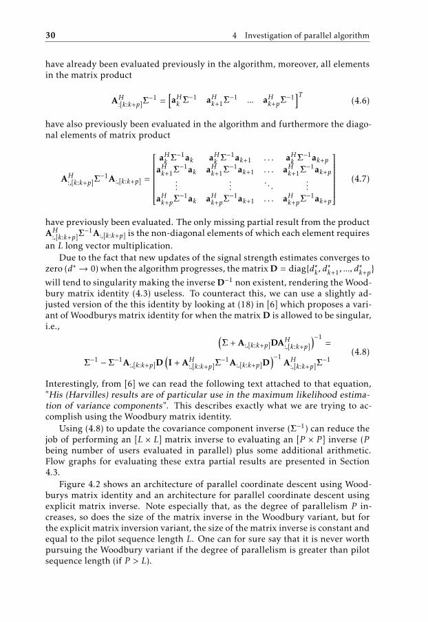
Figure 4.2 shows an architecture of parallel coordinate descent using Wood-burys matrix identity and an architecture for parallel coordinate descent usingexplicit matrix inverse. Note especially that, as the degree of parallelism P in-creases, so does the size of the matrix inverse in the Woodbury variant, but forthe explicit matrix inversion variant, the size of the matrix inverse is constant andequal to the pilot sequence length L. One can for sure say that it is never worthpursuing the Woodbury variant if the degree of parallelism is greater than pilotsequence length (if P > L).

4.3 Flowgraphs for Woodbury architecture 31

CD

CD

CD

D

CD

CD

CD

D

a) b)

+

Woo

dbur

y, [P

x P

]-1

P

[L x L]-1

Figure 4.2: Architecture for parallel coordinate descent using a) the Wood-bury matrix identity approach and b) using an explicit matrix inversion ap-proach.

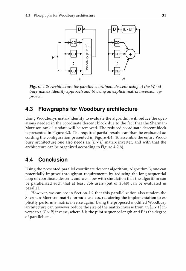
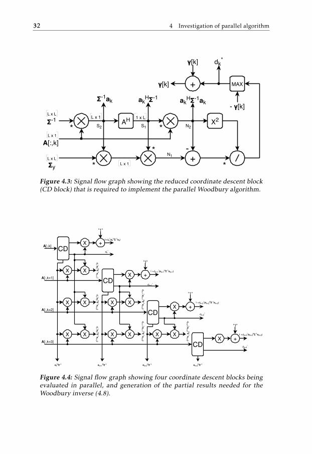
4.3 Flowgraphs for Woodbury architecture

Using Woodburys matrix identity to evaluate the algorithm will reduce the oper-ations needed in the coordinate descent block due to the fact that the Sherman-Morrison rank-1 update will be removed. The reduced coordinate descent blockis presented in Figure 4.3. The required partial results can than be evaluated ac-cording the configuration presented in Figure 4.4. To assemble the entire Wood-bury architecture one also needs an [L × L] matrix inverter, and with that thearchitecture can be organized according to Figure 4.2 b).

4.4 Conclusion

Using the presented parallel coordinate descent algorithm, Algorithm 3, one canpotentially improve throughput requirements by reducing the long sequentialloop of coordinate descent, and we show with simulation that the algorithm canbe parallelized such that at least 256 users (out of 2048) can be evaluated inparallel.

However, we can see in Section 4.2 that this parallelization also renders theSherman-Morrison matrix formula useless, requiering the implementaiton to ex-plicitly perform a matrix inverse again. Using the proposed modified Woodburyarchitecture can however reduce the size of the matrix inverse from an [L × L] in-verse to a [P × P ] inverse, where L is the pilot sequence length and P is the degreeof parallelism.


Σ-1*

AHS2

Σy *

S1

*

*

+N1

N2

-

X2

A[:,k]

MAX

L x 1

L x 1 1 x L

L x L

L x 1

L x L

+γ[k]

γ[k]

*

- γ[k]Σ-1ak akHΣ-1 akHΣ-1ak

dk*

Figure 4.3: Signal flow graph showing the reduced coordinate descent block(CD block) that is required to implement the parallel Woodbury algorithm.

CD

X X

dk*

1+dk*(akHΣ-1ak)

dk *(ak HΣ-1ak+1 )

dk+1*

X

CD

X

CDXX X

X

X X X X

CD

dk+2*

X X

1 +dk+2*(ak+2HΣ-1ak+2)

dk+3*

dk *(ak HΣ-1ak+2 )

dk+1 *(ak+1 HΣ-1ak+2 )

dk *(ak HΣ-1ak+3 )

dk+1 *(ak+1 HΣ-1ak+3 )

dk+2 *(ak+2 HΣ-1ak+3 )

X +

1 +dk+3*(ak+3HΣ-1ak+3)

X +

1 +dk+1*(ak+1HΣ-1ak+1)

+

+A[:,k]

A[:,k+1]

A[:,k+2]

A[:,k+3]

akHΣ-1 ak+1HΣ-1 ak+2HΣ-1 ak+3HΣ-1

"1"

"1"

"1"

"1"

Figure 4.4: Signal flow graph showing four coordinate descent blocks beingevaluated in parallel, and generation of the partial results needed for theWoodbury inverse (4.8).

5Conclusion and final remarks

This chapter will briefly summarize and conclude the results of this project.

5.1 Algorithms

Two algorithms, Algorithms 1 and 2 which are proposed in [5] respective [2], areanalyzed and tuned from a hardware perspective. In Chapter 3 we demonstratesome techniques which can help reduce the size and possibly increase operationfrequency of these algorithms.

Due to the how sequential coordinate descent algorithms are, in Chapter 4, wepropose a parallelized version of the coordinate descent algorithm, Algorithm 3,and through simulation we motivate its viability when compared with Algorithms 1and 2. This altered algorithm have the potential to significantly increase opera-tion frequency of an implementation, but it also comes with some new difficul-ties.

5.2 Implementation

An ASIC implementation in a 28-nm FD-SOI process which evaluates Algorithm 2is produced. The implementation supports Kc = 2048 possible connected users,to a base station with M = 196 antennas and with user pilot sequence lengthsof L = 100. Although the implementation is much to big for actual synthesis,the author later created a new time divided architecture, based on this work, inwhich implementation was successful[7].

In Section 3.4 we present a way of verifying the behavior of the implementa-tion, through model-to-model verification. By making sure that all node valuesmatch between associated models, we verify the behaviour of the VHDL-RTL

33

34 5 Conclusion and final remarks

model, which is finally synthesized to an ASIC implementation. Because of themodel-to-model verification steps, we argue that the final resulting algorithmicperformance of the ASIC implementation can be seen in Figure 3.7.

Appendix

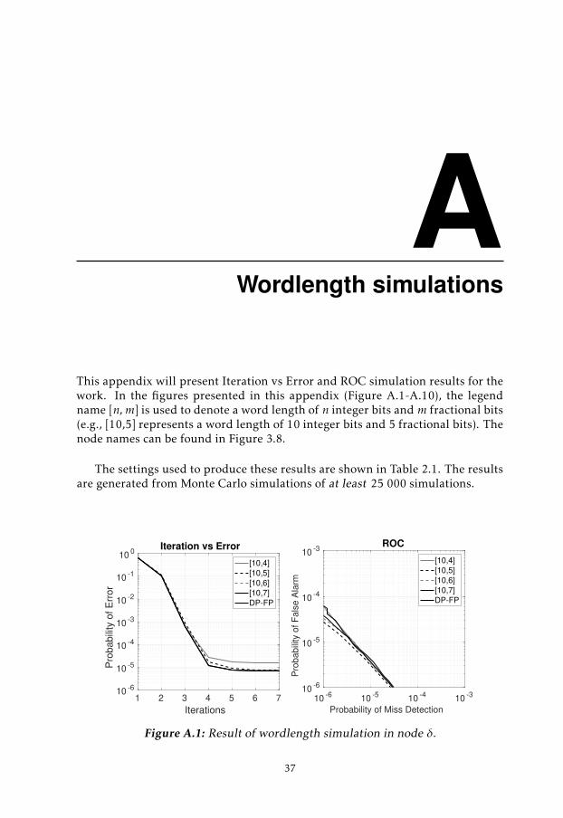
AWordlength simulations

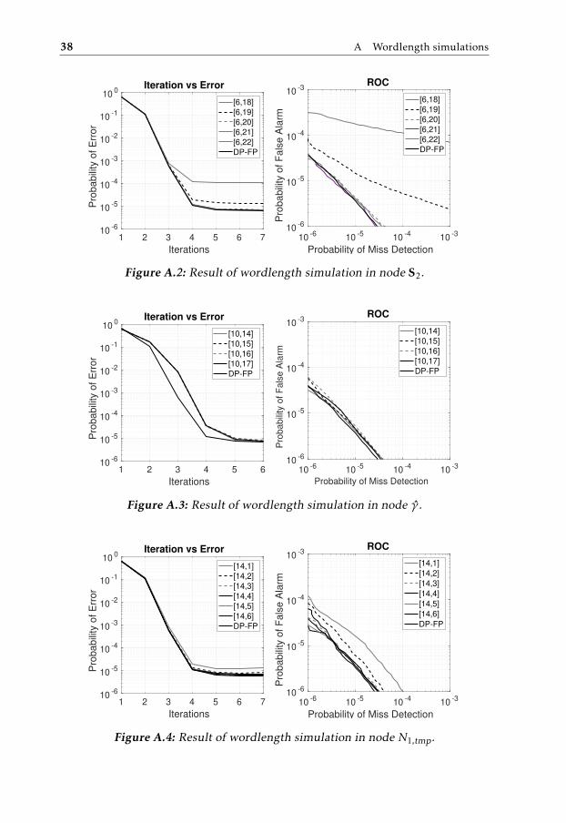
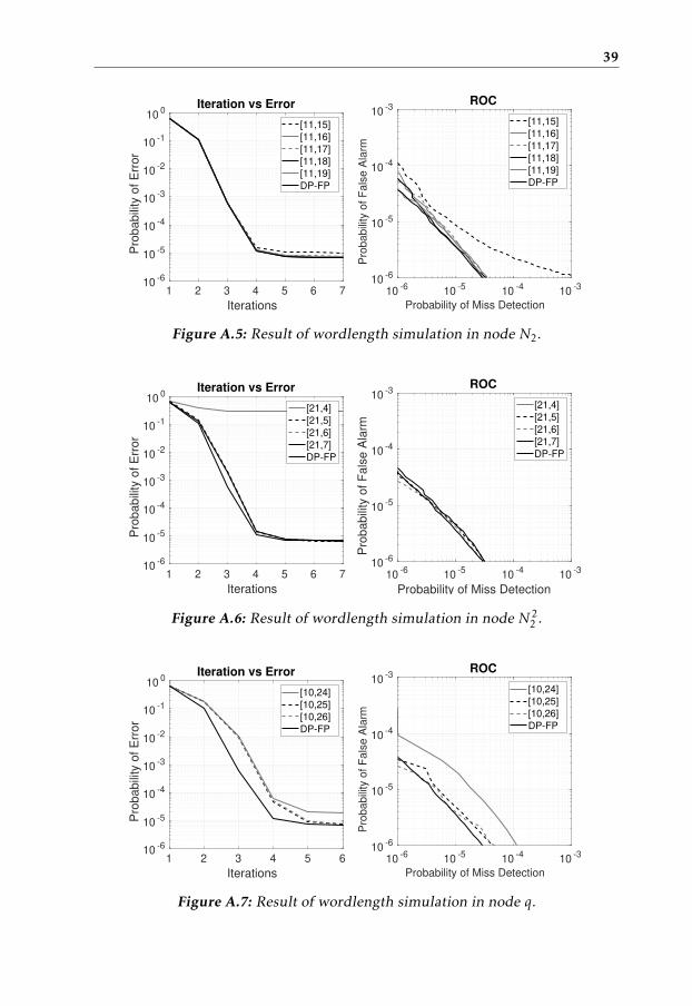
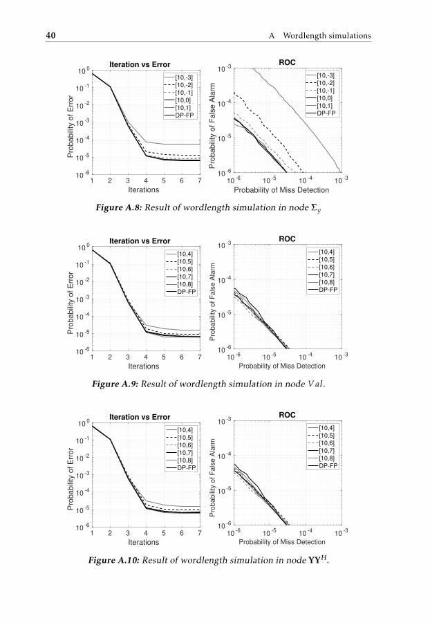
This appendix will present Iteration vs Error and ROC simulation results for thework. In the figures presented in this appendix (Figure A.1-A.10), the legendname [n, m] is used to denote a word length of n integer bits and m fractional bits(e.g., [10,5] represents a word length of 10 integer bits and 5 fractional bits). Thenode names can be found in Figure 3.8.

The settings used to produce these results are shown in Table 2.1. The resultsare generated from Monte Carlo simulations of at least 25 000 simulations.

1 2 3 4 5 6 7

Iterations

10-6

10-5

10-4

10-3

10-2

10-1

100

Pro

babili

ty o

f E

rror

Iteration vs Error

[10,4]

[10,5]

[10,6]

[10,7]

DP-FP

10-6

10-5

10-4

10-3


10-6

10-5

10-4

10-3

Pro

ba

bili

ty o

f F

als

e A

larm

ROC

[10,4]

[10,5]

[10,6]

[10,7]

DP-FP

Figure A.1: Result of wordlength simulation in node δ.

37

38 A Wordlength simulations

1 2 3 4 5 6 7

Iterations

10-6

10-5

10-4

10-3

10-2

10-1

100

Pro

ba

bili

ty o

f E

rro

rIteration vs Error

[6,18]

[6,19]

[6,20]

[6,21]

[6,22]

DP-FP

10-6

10-5

10-4

10-3


10-6

10-5

10-4

10-3

Pro

ba

bili

ty o

f F

als

e A

larm

ROC

[6,18]

[6,19]

[6,20]

[6,21]

[6,22]

DP-FP

Figure A.2: Result of wordlength simulation in node S2.

1 2 3 4 5 6

Iterations

10-6

10-5

10-4

10-3

10-2

10-1

100

Pro

babili

ty o

f E

rror

Iteration vs Error

[10,14]

[10,15]

[10,16]

[10,17]

DP-FP

10-6

10-5

10-4

10-3


10-6

10-5

10-4

10-3

Pro

ba

bili

ty o

f F

als

e A

larm

ROC

[10,14]

[10,15]

[10,16]

[10,17]

DP-FP

Figure A.3: Result of wordlength simulation in node γ .

1 2 3 4 5 6 7

Iterations

10-6

10-5

10-4

10-3

10-2

10-1

100

Pro

babili

ty o

f E

rror

Iteration vs Error

[14,1]

[14,2]

[14,3]

[14,4]

[14,5]

[14,6]

DP-FP

10-6

10-5

10-4

10-3


10-6

10-5

10-4

10-3

Pro

babili

ty o

f F

als

e A

larm

ROC

[14,1]

[14,2]

[14,3]

[14,4]

[14,5]

[14,6]

DP-FP

Figure A.4: Result of wordlength simulation in node N1,tmp.

39

1 2 3 4 5 6 7

Iterations

10-6

10-5

10-4

10-3

10-2

10-1

100

Pro

babili

ty o

f E

rror

Iteration vs Error

[11,15]

[11,16]

[11,17]

[11,18]

[11,19]

DP-FP

10-6

10-5

10-4

10-3


10-6

10-5

10-4

10-3

Pro

ba

bili

ty o

f F

als

e A

larm

ROC

[11,15]

[11,16]

[11,17]

[11,18]

[11,19]

DP-FP

Figure A.5: Result of wordlength simulation in node N2.

1 2 3 4 5 6 7

Iterations

10-6

10-5

10-4

10-3

10-2

10-1

100

Pro

babili

ty o

f E

rror

Iteration vs Error

[21,4]

[21,5]

[21,6]

[21,7]

DP-FP

10-6

10-5

10-4

10-3


10-6

10-5

10-4

10-3

Pro

babili

ty o

f F

als

e A

larm

ROC

[21,4]

[21,5]

[21,6]

[21,7]

DP-FP

Figure A.6: Result of wordlength simulation in node N22 .

1 2 3 4 5 6

Iterations

10-6

10-5

10-4

10-3

10-2

10-1

100

Pro

babili

ty o

f E

rror

Iteration vs Error

[10,24]

[10,25]

[10,26]

DP-FP

10-6

10-5

10-4

10-3


10-6

10-5

10-4

10-3

Pro

ba

bili

ty o

f F

als

e A

larm

ROC

[10,24]

[10,25]

[10,26]

DP-FP

Figure A.7: Result of wordlength simulation in node q.

40 A Wordlength simulations

1 2 3 4 5 6 7

Iterations

10-6

10-5

10-4

10-3

10-2

10-1

100

Pro

babili

ty o

f E

rror

Iteration vs Error

[10,-3]

[10,-2]

[10,-1]

[10,0]

[10,1]

DP-FP

10-6

10-5

10-4

10-3


10-6

10-5

10-4

10-3

Pro

babili

ty o

f F

als

e A

larm

ROC

[10,-3]

[10,-2]

[10,-1]

[10,0]

[10,1]

DP-FP

Figure A.8: Result of wordlength simulation in node Σy

1 2 3 4 5 6 7

Iterations

10-6

10-5

10-4

10-3

10-2

10-1

100

Pro

babili

ty o

f E

rror

Iteration vs Error

[10,4]

[10,5]

[10,6]

[10,7]

[10,8]

DP-FP

10-6

10-5

10-4

10-3


10-6

10-5

10-4

10-3

Pro

ba

bili

ty o

f F

als

e A

larm

ROC

[10,4]

[10,5]

[10,6]

[10,7]

[10,8]

DP-FP

Figure A.9: Result of wordlength simulation in node V al.

1 2 3 4 5 6 7

Iterations

10-6

10-5

10-4

10-3

10-2

10-1

100

Pro

babili

ty o

f E

rror

Iteration vs Error

[10,4]

[10,5]

[10,6]

[10,7]

[10,8]

DP-FP

10-6

10-5

10-4

10-3


10-6

10-5

10-4

10-3

Pro

ba

bili

ty o

f F

als

e A

larm

ROC

[10,4]

[10,5]

[10,6]

[10,7]

[10,8]

DP-FP

Figure A.10: Result of wordlength simulation in node YYH.

BInitial MATLAB model

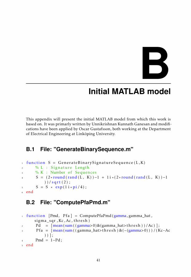
This appendix will present the initial MATLAB model from which this work isbased on. It was primarly written by Unnikrishnan Kunnath Ganesan and modifi-cations have been applied by Oscar Gustafsson, both working at the Departmentof Electrical Engineering at Linköping University.

B.1 File: "GenerateBinarySequence.m"

1 funct ion S = GenerateBinarySignatureSequence ( L ,K)2 % L : Signature Length3 % K : Number of Sequences4 S = (2* round ( rand ( L , K) ) −1 + 1 i * ( 2 * round ( rand ( L , K) ) −1

) ) / s q r t ( 2 ) ;5 S = S * exp (1 i * pi /4) ;6 end

B.2 File: "ComputePfaPmd.m"

1 funct ion [Pmd, Pfa ] = ComputePfaPmd (gamma, gamma_hat ,sigma_sqr , Kc , Ac , thresh )

2 Pd = [ mean(sum ( ( gamma>0)&(gamma_hat>thresh ) ) /Ac ) ] ;3 Pfa = [ mean(sum ( ( gamma_hat>thresh ) &(~(gamma>0) ) ) / ( Kc−Ac

) ) ] ;4 Pmd = 1−Pd ;5 end

41

42 B Initial MATLAB model

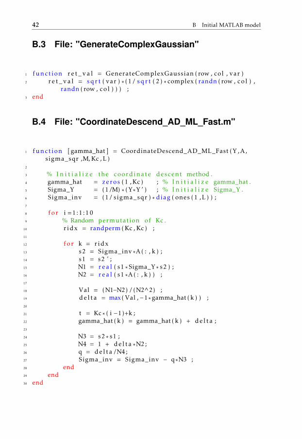
B.3 File: "GenerateComplexGaussian"

1 funct ion r e t _ v a l = GenerateComplexGaussian ( row , col , var )2 r e t _ v a l = s q r t ( var ) * (1/ s q r t ( 2 ) * complex ( randn ( row , co l ) ,

randn ( row , co l ) ) ) ;3 end

B.4 File: "CoordinateDescend_AD_ML_Fast.m"

1 funct ion [ gamma_hat ] = CoordinateDescend_AD_ML_Fast (Y ,A,sigma_sqr ,M, Kc , L )

2

3 % I n i t i a l i z e the coordinate descent method .4 gamma_hat = zeros ( 1 , Kc ) ; % I n i t i a l i z e gamma_hat .5 Sigma_Y = (1/M) * (Y*Y ’ ) ; % I n i t i a l i z e Sigma_Y .6 Sigma_inv = (1/ sigma_sqr ) * diag ( ones ( 1 ,L ) ) ;7

8 for i =1:1:109 % Random permutation of Kc .

10 r idx = randperm ( Kc , Kc ) ;11

12 fo r k = ridx13 s2 = Sigma_inv *A( : , k ) ;14 s1 = s2 ’ ;15 N1 = r e a l ( s1 *Sigma_Y* s2 ) ;16 N2 = r e a l ( s1 *A( : , k ) ) ;17

18 Val = (N1−N2) / (N2^2) ;19 d e l t a = max( Val , −1*gamma_hat ( k ) ) ;20

21 t = Kc * ( i −1)+k ;22 gamma_hat ( k ) = gamma_hat ( k ) + d e l t a ;23

24 N3 = s2 * s1 ;25 N4 = 1 + d e l t a *N2 ;26 q = d e l t a /N4 ;27 Sigma_inv = Sigma_inv − q*N3 ;28 end29 end30 end

B.5 File: "CoordinateDescent.m" 43

B.5 File: "CoordinateDescent.m"

1 M = 196 ; % No of Antennas at Base S t a t i o n .2 Kc = 2048 ; % No of P o t e n t i a l Users .3 Ac = 200 ; % Active Users .4 L = 100 ; % P i l o t Dimension , a l s o know as Dc .5 SNR = 10 ; % Signal to noise r a t i o [ dB ] .6 sigma_sqr = 1/SNR ; % Noise var iance .7

8 % Signature Sequence .9 Acand = { GenerateBinarySignatureSequence (L , Kc ) } ;

10 A = Acand { 1 } ;11

12 % Monte c a r l o s imulat ions to perform .13 monte = 500 ;14

15 % Threshold values .16 threshold = 0 . 0 0 5 : 0 . 0 0 5 : 1 . 0 ;17

18 % Create gamma v e c t o r s for comparison .19 gamma = zeros ( monte , Kc ) ;20 gamma_hat = zeros ( monte , Kc ) ;21

22 %23 % Main simulat ion loop .24 %25 parfor i = 1 : monte26

27 % Fading Channel Model .28 H = GenerateComplexGaussian ( Kc ,M, 1 ) ;29

30 % Active User L i s t . Kc from a t o t a l of Ac .31 A c _ l i s t = randperm ( Kc , Ac ) ;32

33 % Transmitted Signal .34 v = zeros ( 1 , Kc ) ;35 v ( A c _ l i s t ) = 1 ; % Signal power = 1 .36 gamma( i , : ) = v ; % Assign Tx power to devices .37 Gamma_sqrt = diag ( s q r t (gamma( i , : ) ) ) ;38 Z = GenerateComplexGaussian (L ,M, sigma_sqr ) ;39 Y = A*Gamma_sqrt*H + Z ;40

41 % Run simulat ion .42 gamma_hat ( i , : ) = CoordinateDescend_AD_ML_Fast (Y ,A,

sigma_sqr ,M, Kc , L ) ;43 end

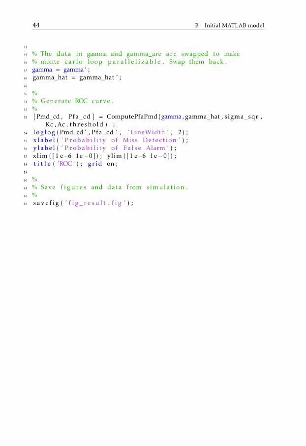
44 B Initial MATLAB model

44

45 % The data in gamma and gamma_are are swapped to make46 % monte c a r l o loop p a r a l l e l i z a b l e . Swap them back .47 gamma = gamma ’ ;48 gamma_hat = gamma_hat ’ ;49

50 %51 % Generate ROC curve .52 %53 [ Pmd_cd , Pfa_cd ] = ComputePfaPmd (gamma, gamma_hat , sigma_sqr ,

Kc , Ac , threshold ) ;54 log log (Pmd_cd ’ , Pfa_cd ’ , ’ LineWidth ’ , 2) ;55 x l a b e l ( ’ P r o b a b i l i t y of Miss Detect ion ’ ) ;56 y l a b e l ( ’ P r o b a b i l i t y of Fa l se Alarm ’ ) ;57 xlim ( [ 1 e−6 1e −0]) ; ylim ( [ 1 e−6 1e −0] ) ;58 t i t l e ( ’ROC’ ) ; gr id on ;59

60 %61 % Save f i g u r e s and data from simulat ion .62 %63 s a v e f i g ( ’ f i g _ r e s u l t . f i g ’ ) ;

Bibliography

[1] E. Björnson, L. Sanguinetti, and M. Debbah. Massive MIMO with imperfectchannel covariance information. In 50th Asilomar Conference on Signals,Systems and Computers, pages 974–978, 2016.

[2] Z. Chen, F. Sohrabi, Y. Liu, and W. Yu. Covariance based joint activity anddata detection for massive random access with massive MIMO. In IEEEInternational Conference on Communications (ICC), pages 1–6, May 2019.doi: 10.1109/ICC.2019.8761672.

[3] Jialin Dong, Jun Zhang, Yuanming Shi, and Jessie Hui Wang. Faster activ-ity and data detection in massive random access: A multi-armed bandit ap-proach. arXiv e-prints, art. arXiv:2001.10237, January 2020.

[4] Mert Gurbuzbalaban, Asuman Ozdaglar, Nuri Denizcan Vanli, andStephen J. Wright. Randomness and permutations in coordinate descentmethods. arXiv e-prints, art. arXiv:1803.08200, March 2018.

[5] Saeid Haghighatshoar, Peter Jung, and Giuseppe Caire. A new scalinglaw for activity detection in massive mimo systems. arXiv e-prints, art.arXiv:1803.02288, March 2018.

[6] H. V. Henderson and S. R. Searle. On deriving the inverse of a sum ofmatrices. SIAM Review, 23(1):53–60, 1981. ISSN 00361445. URL http://www.jstor.org/stable/2029838.

[7] M. Henriksson, O. Gustafsson, U. K. Ganesan, and E. G. Larsson. An archi-tecture for grant-free random access massive machine type communicationusing coordinate descent. In Proceedings of 54th Asilomar Conference onSignals, Systems, and Computers. IEEE, 2020.

[8] L. Liu, E. G. Larsson, W. Yu, P. Popovski, C. Stefanovic, and E. de Car-valho. Sparse signal processing for grant-free massive connectivity: A futureparadigm for random access protocols in the internet of things. IEEE SignalProcessing Magazine, 35(5):88–99, September 2018. ISSN 1558-0792. doi:10.1109/MSP.2018.2844952.

45

http://www.jstor.org/stable/2029838

http://www.jstor.org/stable/2029838

46 Bibliography

[9] D. Menard, G. Caffarena, J. A. Lopez, D. Novo, and O. Sentieys. Anal-ysis of finite word-length effects in fixed-point systems. In Shuvra S.Bhattacharyya, Ed F. Deprettere, Rainer Leupers, and Jarmo Takala, edi-tors, Handbook of Signal Processing Systems, pages 1063–1101. SpringerInternational Publishing, Cham, 2019. ISBN 978-3-319-91734-4. doi:10.1007/978-3-319-91734-4_29.

[10] Peter Richtárik and Martin Takáč. Parallel coordinate descent methods forbig data optimization. arXiv e-prints, art. arXiv:1212.0873, December 2012.

[11] N. M. Sarband, E. Becirovic, M. Krysander, E. G. Larsson, and O. Gustafs-son. Pilot-hopping sequence detection architecture for grant-free randomaccess using massive MIMO. In IEEE International Symposium on Circuitsand Systems (ISCAS), pages 1–5, 2020. doi: 10.1109/ISCAS45731.2020.9180888.

[12] Jack Sherman and Winifred J. Morrison. Adjustment of an Inverse MatrixCorresponding to a Change in One Element of a Given Matrix. Ann. Math.Statist., 21(1):124–127, 03 1950. doi: 10.1214/aoms/1177729893.

[13] M. Tran, O. Gustafsson, P. Källström, K. Şenel, and E. G. Larsson. An archi-tecture for grant-free massive MIMO MTC based on compressive sensing.In 53rd Asilomar Conference on Signals, Systems, and Computers, pages901–905, 2019. doi: 10.1109/IEEECONF44664.2019.9048663.

[14] F. Vahid. Digital Design with RTL Design, VHDL, and Verilog. Wiley,2010. ISBN 9780470531082. URL https://books.google.se/books?id=-YayRpmjc20C.

https://books.google.se/books?id=-YayRpmjc20C

https://books.google.se/books?id=-YayRpmjc20C

Documents

Implementation of a Hardware Coordinate Wise Descend