Embed Size (px)
Citation preview
Fukuoka Institute of Technology
Graduate School of Engineering
Implementation of a Testbed and a
Simulation System for MANETs:
Experiments and Simulations
by
Elis KULLA
Adviser: Prof. Leonard Barolli
2013
Contents
List of Figures ii
List of Tables iii
Acknowledgement v
Abstract vii
1 Introduction 1
1.1 Background . . . . . . . . . . . . . . . . . . . . . . . . . . . . . . . . 1
1.2 Research Background and Related Work . . . . . . . . . . . . . . . . 3
1.3 The Structure Of The Thesis . . . . . . . . . . . . . . . . . . . . . . 5
2 Wireless Networks 7
2.1 Introduction . . . . . . . . . . . . . . . . . . . . . . . . . . . . . . . . 7
2.2 Wireless Architecture . . . . . . . . . . . . . . . . . . . . . . . . . . . 7
2.2.1 Infrastracture Architecture . . . . . . . . . . . . . . . . . . . . 7
2.2.2 Ad Hoc Architecture . . . . . . . . . . . . . . . . . . . . . . . 8
2.3 Wireless vs. Wired . . . . . . . . . . . . . . . . . . . . . . . . . . . . 9
2.3.1 Collision . . . . . . . . . . . . . . . . . . . . . . . . . . . . . . 9
2.3.2 Unidirectional Links . . . . . . . . . . . . . . . . . . . . . . . 9
2.3.3 Asymmetric Links . . . . . . . . . . . . . . . . . . . . . . . . 10
2.4 The Wireless Channel . . . . . . . . . . . . . . . . . . . . . . . . . . 10
2.4.1 Free Space Propagation Model . . . . . . . . . . . . . . . . . . 11
2.4.2 Two-Ray Ground Model . . . . . . . . . . . . . . . . . . . . . 11
2.4.3 Shadowing Model . . . . . . . . . . . . . . . . . . . . . . . . 13
2.5 Wireless Technologies . . . . . . . . . . . . . . . . . . . . . . . . . . . 13
i
Contents
2.5.1 Wi-Fi . . . . . . . . . . . . . . . . . . . . . . . . . . . . . . . 13
2.5.2 WiMAX . . . . . . . . . . . . . . . . . . . . . . . . . . . . . . 14
2.5.3 Bluetooth . . . . . . . . . . . . . . . . . . . . . . . . . . . . . 14
2.5.4 4G Cellular Networks . . . . . . . . . . . . . . . . . . . . . . . 15
2.5.5 MANETs . . . . . . . . . . . . . . . . . . . . . . . . . . . . . 15
3 MANET 17
3.1 MANETs Usage and Applications . . . . . . . . . . . . . . . . . . . . 18
3.2 MANETs Challenges . . . . . . . . . . . . . . . . . . . . . . . . . . . 19
3.3 Routing in MANETs . . . . . . . . . . . . . . . . . . . . . . . . . . . 20
3.3.1 Proactive Routing . . . . . . . . . . . . . . . . . . . . . . . . . 21
3.3.1.1 Optimized Link State Routing (RFC3626) . . . . . . 22
3.3.1.2 Better Approach To MANET (BATMAN) . . . . . . 24
3.3.2 Reactive Routing . . . . . . . . . . . . . . . . . . . . . . . . . 25
3.3.2.1 Ad hoc On-Demand Distance Vector (RFC 3561) . . 26
3.3.3 Adaptive and Hybrid Routing Protocols . . . . . . . . . . . . 27
3.4 MANET Research Tools . . . . . . . . . . . . . . . . . . . . . . . . . 27
3.4.1 Evaluation Techniques . . . . . . . . . . . . . . . . . . . . . . 28
3.4.1.1 Simulations . . . . . . . . . . . . . . . . . . . . . . . 28
3.4.1.2 Emulators . . . . . . . . . . . . . . . . . . . . . . . . 28
3.4.1.3 Real-World Testbeds . . . . . . . . . . . . . . . . . . 29
3.4.2 Mobility in MANETs . . . . . . . . . . . . . . . . . . . . . . . 29
3.4.3 Real Testbeds with Mobility . . . . . . . . . . . . . . . . . . 30
3.4.4 Discussion . . . . . . . . . . . . . . . . . . . . . . . . . . . . 32
4 Testbed Implementation and Experimental Scenarios 35
4.1 Testbed Design and Implementation . . . . . . . . . . . . . . . . . . . 35
4.1.1 Description . . . . . . . . . . . . . . . . . . . . . . . . . . . . 35
4.1.2 Testbed Interface . . . . . . . . . . . . . . . . . . . . . . . . . 36
4.1.3 Testbed Environment . . . . . . . . . . . . . . . . . . . . . . . 36
4.2 Experimental Scenarios . . . . . . . . . . . . . . . . . . . . . . . . . . 37
4.2.1 Case 1: Indoor Stairs . . . . . . . . . . . . . . . . . . . . . . . 37
4.2.2 Case 2: Outdoor Bridge . . . . . . . . . . . . . . . . . . . . . 37
4.2.3 Case 3: Indoor Multimedia . . . . . . . . . . . . . . . . . . . . 39
ii Elis KULLA
Contents
5 Simulators and Simulation Scenarios 43
5.1 NS2 Simulator System . . . . . . . . . . . . . . . . . . . . . . . . . . 43
5.1.1 Introduction . . . . . . . . . . . . . . . . . . . . . . . . . . . . 43
5.1.2 Mobility Models . . . . . . . . . . . . . . . . . . . . . . . . . . 44
5.1.2.1 Random Waypoint Mobility (RWM) model . . . . . 44
5.1.2.2 2D Random Walk Mobility Model (RW2) . . . . . . 44
5.2 Simulation Scenarios . . . . . . . . . . . . . . . . . . . . . . . . . . . 44
5.2.1 Case 1: Static2, OLSR and AODV . . . . . . . . . . . . . . . 44
5.2.2 Case 2: Static2, Static4, Static9 . . . . . . . . . . . . . . . . . 45
5.2.3 Case 3: RREQ, RREP, RERR, HELLO for AODV . . . . . . 47
5.2.4 Case 4: Data Replication in MANET . . . . . . . . . . . . . . 47
5.2.4.1 Simulation Parameters . . . . . . . . . . . . . . . . . 49
5.2.4.2 Proposed Fuzzy-based Data Replication System . . . 50
6 Experimental Results 55
6.1 Case1: Indoor Stairs . . . . . . . . . . . . . . . . . . . . . . . . . . . 55
6.2 Case2: Outdoor Bridge . . . . . . . . . . . . . . . . . . . . . . . . . . 58
6.3 Case3: Multimedia Transmissions . . . . . . . . . . . . . . . . . . . . 59
7 Simulation Results 63
7.1 Case 1: Static Source and Destination for OLSR and AODV . . . . . 63
7.2 Case 2: Static2, Static4, Static9 . . . . . . . . . . . . . . . . . . . . . 68
7.3 Case 3: RREQ, RERR, RREP, HELLO for AODV . . . . . . . . . . 71
7.4 Case 4: Data Replication . . . . . . . . . . . . . . . . . . . . . . . . . 74
8 Conclusions and Future Works 77
8.1 Conclusions . . . . . . . . . . . . . . . . . . . . . . . . . . . . . . . . 77
8.1.1 Experiments . . . . . . . . . . . . . . . . . . . . . . . . . . . . 78
8.1.1.1 Case 1 . . . . . . . . . . . . . . . . . . . . . . . . . . 78
8.1.1.2 Case 2 . . . . . . . . . . . . . . . . . . . . . . . . . . 78
8.1.1.3 Case 3 . . . . . . . . . . . . . . . . . . . . . . . . . . 79
8.1.2 Simulations . . . . . . . . . . . . . . . . . . . . . . . . . . . . 79
8.1.2.1 Case 1 . . . . . . . . . . . . . . . . . . . . . . . . . . 79
8.1.2.2 Case 2 . . . . . . . . . . . . . . . . . . . . . . . . . . 80
8.1.2.3 Case 3 . . . . . . . . . . . . . . . . . . . . . . . . . . 80
iii Elis KULLA

Contents
8.1.2.4 Case 4 . . . . . . . . . . . . . . . . . . . . . . . . . . 81
8.2 Future Works . . . . . . . . . . . . . . . . . . . . . . . . . . . . . . . 82
References 83
List of Papers 94
iv Elis KULLA
List of Figures
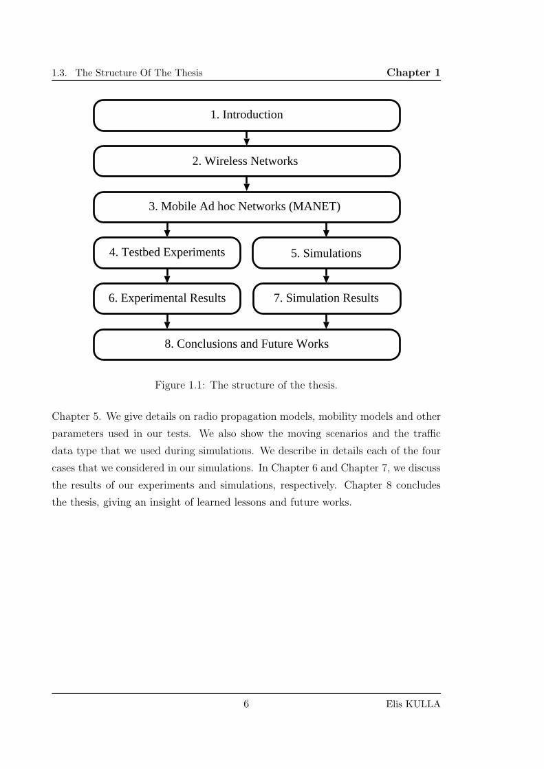
1.1 The structure of the thesis. . . . . . . . . . . . . . . . . . . . . . . . . 6
2.1 Ad-Hoc and infrastructure mode. . . . . . . . . . . . . . . . . . . . . 8
2.2 Two-ray Ground Propagation Model. . . . . . . . . . . . . . . . . . . 12
3.1 MPRs selection, reaching all 2-hop neighbors . . . . . . . . . . . . . . 23
4.1 Testbed interface. . . . . . . . . . . . . . . . . . . . . . . . . . . . . . 36
4.2 Snapshots of nodes for indoor vertical scenarios. . . . . . . . . . . . . 38
4.3 Indoor vertical scenarios. . . . . . . . . . . . . . . . . . . . . . . . . . 39
4.4 Outdoor bridge scenarios. . . . . . . . . . . . . . . . . . . . . . . . . 40
4.5 Node positioning and MAC filtering for LT. . . . . . . . . . . . . . . 40
5.1 Node positions. . . . . . . . . . . . . . . . . . . . . . . . . . . . . . . 46
5.2 Simulation scenarios. . . . . . . . . . . . . . . . . . . . . . . . . . . . 48
5.3 Input and Output of the FDRM System. . . . . . . . . . . . . . . . . 51
5.4 FLC structure. . . . . . . . . . . . . . . . . . . . . . . . . . . . . . . 51
5.5 Triangular and trapezoidal membership functions. . . . . . . . . . . . 52
5.6 Membership functions. . . . . . . . . . . . . . . . . . . . . . . . . . . 52
6.1 Throughput results. . . . . . . . . . . . . . . . . . . . . . . . . . . . . 56
6.2 Delay results. . . . . . . . . . . . . . . . . . . . . . . . . . . . . . . . 57
6.3 Packetloss results for STAS and SHIS scenarios. . . . . . . . . . . . . 58
6.4 Bitrate experimental results. . . . . . . . . . . . . . . . . . . . . . . . 60
6.5 Packetloss experimental results. . . . . . . . . . . . . . . . . . . . . . 61
6.6 Throughput results. . . . . . . . . . . . . . . . . . . . . . . . . . . . . 62
7.1 Distance vs. Nr. of Hops (ALMOV). . . . . . . . . . . . . . . . . . . 64
v
List of Figures
7.2 Distance vs. Nr. of Hops (SDSTA). . . . . . . . . . . . . . . . . . . . 65
7.3 Throughput vs. Nr. of Hops OLSR (ALMOV). . . . . . . . . . . . . 66
7.4 Throughput vs. Nr. of Hops OLSR (SDSTA). . . . . . . . . . . . . . 66
7.5 Throughput vs. Nr. of Hops AODV (ALMOV). . . . . . . . . . . . . 67
7.6 Throughput vs. Nr. of Hops AODV (SDSTA). . . . . . . . . . . . . . 67
7.7 Throughput vs. Number of Hops (Static2) . . . . . . . . . . . . . . . 69
7.8 Throughput vs. Number of Hops (Static4) . . . . . . . . . . . . . . . 69
7.9 Throughput vs. Number of Hops (Static9) . . . . . . . . . . . . . . . 70
7.10 Results for AODV packets. . . . . . . . . . . . . . . . . . . . . . . . . 71
7.11 RERR Packet Rate. . . . . . . . . . . . . . . . . . . . . . . . . . . . . 72
7.12 Average throughput. . . . . . . . . . . . . . . . . . . . . . . . . . . . 72
7.13 Throughput results. . . . . . . . . . . . . . . . . . . . . . . . . . . . . 73
7.14 FDRM system results. . . . . . . . . . . . . . . . . . . . . . . . . . . 75
vi Elis KULLA
List of Tables
2.1 Values of the path loss exponent in different environments. . . . . . . 13
3.1 Testbeds characteristics. . . . . . . . . . . . . . . . . . . . . . . . . . 31
4.1 Experimental parameters. . . . . . . . . . . . . . . . . . . . . . . . . 38
4.2 Experimental parameters. . . . . . . . . . . . . . . . . . . . . . . . . 39
4.3 Experimental parameters. . . . . . . . . . . . . . . . . . . . . . . . . 41
5.1 Simulation Settings. . . . . . . . . . . . . . . . . . . . . . . . . . . . . 45
5.2 Simulation Settings. . . . . . . . . . . . . . . . . . . . . . . . . . . . . 46
5.3 Simulation Settings. . . . . . . . . . . . . . . . . . . . . . . . . . . . . 48
5.4 Simulation Settings for Case 3. . . . . . . . . . . . . . . . . . . . . . 49
5.5 Parameters and their term sets. . . . . . . . . . . . . . . . . . . . . . 53
5.6 Fuzzy Rule Base. . . . . . . . . . . . . . . . . . . . . . . . . . . . . . 54
6.1 Average throughput (kbit/s). . . . . . . . . . . . . . . . . . . . . . . 56
6.2 Average delay (s). . . . . . . . . . . . . . . . . . . . . . . . . . . . . . 57
6.3 Average Packetloss (pps). . . . . . . . . . . . . . . . . . . . . . . . . 57
6.4 Throughput results (kbit/s). . . . . . . . . . . . . . . . . . . . . . . . 61
6.5 Delay results (s). . . . . . . . . . . . . . . . . . . . . . . . . . . . . . 62
6.6 Packetloss results (pps). . . . . . . . . . . . . . . . . . . . . . . . . . 62
7.1 Average throughput values for ALMOV Scenario. . . . . . . . . . . . 64
7.2 Average values for SDSTA Scenario. . . . . . . . . . . . . . . . . . . . 64
vii

Acknowledgement
Working three years to complete my Ph.D. course was not an easy task. The support
of many people was crucial and without them this thesis would be very difficult.
First, I would like to thank my adviser, Professor Leonard Barolli, for his con-
tinuous efforts and support. He was always ready to listen and to advice. He taught
me how to be practical and persistent in my projects without giving up. Without
his consistency and insistence, the completion of this work would be impossible.
I thank Professor Kazunori Uchida for his every-week comments and support
about my research and life. I want to thank Professor Jiro Iwashige for his kind
support in difficult days. With his everyday technical recommendations and advice,
Dr. Makoto Ikeda was always there. Thank you Dr. Ikeda. With the support of
Ms. Sawako Tsunenoki and Mrs. Hiroko Yoshida, I overpassed the tough process of
document submission and institutional procedures in Japan.
A special thank goes to Professor Makoto Takizawa (Hosei University, Japan),
who always supported me spiritually and gave a lot of feedback. I also thank Pro-
fessor Fatos Xhafa (Technical University of Catalonia, Spain) for his long talks and
innovative ideas in my research field.
My research in Fukuoka Institute of Technology was also inspired by my col-
leagues. I would also like to thank my colleague, Ms. Evjola Spaho next desk, for
her practical advice and moral support during these three busy years. My thanks
go also to Mr. Masahiro Hiyama and all students of INA Lab studying for endless
hours in the laboratory, inspiring me to work harder.
Finally I would like to thank my parents, Sami and Doloreza, my brother Bernard
and my sister Eriola, for supporting me with emails and skype talks. Therefore, I
want to dedicate this thesis to my beloved family. Their educational support is
priceless.
ix

Abstract
A Mobile Ad hoc Network (MANET) can be defined as a collection of mobile nodes,
which form a highly resource constrained network and a dynamic topology. Because
of the dynamic topology, routing procedures and protocols are a key field of testing
and research. In a research environment, research tools are required to test, verify
and identify problems of an algorithm or protocol. These tools are classified in
three major techniques: simulators, emulators and real-world testbeds. In most
of research in MANET, their performance is evaluated in both quantitative and
qualitative aspects. Throughput performance, routing efficiency, security and energy
consumption are some of the key issues that are addressed frequently on MANETs.
The future MANET technology will have to ensure a certain degree of security and
scalability and provide the infrastructure for collaborative computing. In this thesis,
we design and implement a testbed and a simulation system in order to analyze the
performance and compare the results of different routing protocols, mobility models
and other environmental parameters. In both approaches we use different models,
scenarios and traffic data models. We use our simulation results to improve the
experimental environment. We experimented in indoor and outdoor environment, in
horizontal and vertical topologies and in linear and mesh logical topologies. We also
added mobility to specific nodes. From results, we found that the mobility of nodes
brings oscillations in performance and route instabilities. Using our simulation tool,
we simulated different mobility patterns in different protocols. We found multi-flow
traffic decreases the performance of the network. We also proposed a data replication
framework based on fuzzy logic to improve QoS in MANET. From simulation results,
we found that the proposed framework had a good performance. The contributions
of our work are:
1. Implementation and evaluation of a MANET testbed;
xi
Abstract
2. Implementation of a simulation tool for MANETs using NS2;
3. Application of MANET testbed in real environments, considering different
scenarios;
4. Evaluation of different MANET routing protocols in different scenarios;
5. Propose a new data replication framework for improving QoS in MANET;
6. Give insights about future developments and integration of MANET as an
important technology of wireless communications.
The outline of the thesis is as follows. In Chapter 1, is shown the background
and the motivation of the thesis. In Chapter 2, we introduce general aspects of
wireless networks. We discuss wireless architectures and wireless technologies giving
advantages and disadvantages of each. We give insights of MANETs in Chapter 3.
We discuss issues and problems of MANETs, and describe routing protocols and
their properties. In Chapter 4, we present the design and implementation of our
testbed. We give details on technical settings and environment assumptions. The
scenarios and the way of implementation are described in details. The simulation
system is presented in Chapter 5. We give details on radio propagation models,
mobility models and other parameters used in our tests. Later we show the moving
scenarios and the traffic data that we used during simulations. In Chapter 6 and
Chapter 7, we discuss the results of our experiments and simulations, respectively.
Chapter 8 concludes the thesis, giving an insight of learned lessons and future works
in this field.
xii Elis KULLA
Chapter 1
Introduction
1.1 Background
The increasing need of users for communications and to access information any-
time and anywhere, has made wireless mobile networks become very popular. The
everyday-life wireless networks are often connected to a wired network at some
points, even though the users are not aware of that fact. A wired backbone infras-
tructure is needed, in order for these networks to access certain resources or reach
other networks and devices. The case of mobile telephony shows the above men-
tioned need, where each mobile host connects wireless with a base station on the
wired network, with one-hop radio transmissions. Whereas, Mobile Ad Hoc Net-
works (MANETs), communicate in a different philosophy. A MANET is a bunch
of wireless mobile devices, that can create a temporary or one-purpose (Ad Hoc)
network, without any support from wired network resources. The wireless devices
in MANETs, from now on in this paper referred as nodes, create communication
paths with each other via one-hop or multi-hop links, in a peer-to-peer design. Each
node in between a communication path acts as a router. Thus, the nodes should be
able to operate as end-to-end devices and routers. Another feature of MANETs is
the nodes random mobility, which brings the creation of different routing paths as
time changes. Also, the topology of the network changes continuously. Thus, the
addition and deletion of nodes from the topology need to be handled.
Recently, MANETs are continuing to attract the attention for their applications
in several fields, where the communication infrastructure is expensive and/or time
consuming. Mobility and the absence of any fixed infrastructure make MANET very
1
1.1. Background Chapter 1
attractive for rescue operations and time-critical applications. Communications in
battlefields, disaster recovery areas or in other time-critical environments are good
examples of MANET usage and applications. For example, in an area affected by a
disaster, the creation of a quick communication network, is very important in order
for the public safety agencies and rescue teams can share critical information for the
situation.
More specific MANETs, that have attracted a great amount of research interests,
are Wireless Sensor Networks (WSNs) and Vehicular Ad-hoc Networks (VANETs).
WSNs are MANETs consisting of sensor nodes and serve to measure some environ-
mental parameter, and collect the information in special nodes called sinks. VANETs
are MANETs with the special feature of conditional movement, modeling lanes of
a road. Research for MANETs has been done usually in simulation, because in
general, a simulator can give a quick and inexpensive evaluation of protocols and
algorithms. However, experimentations in the real world are very important to ver-
ify the simulation results and to revise the models implemented in the simulator. A
typical example of this approach has revealed many aspects of IEEE 802.11, like the
gray-zones effect [1], which usually are not taken into account in standard simulators,
as the well-known ns-2 simulator.
We conducted many experiments with our MANET testbed [2,3]. We proved that
while some of the Optimized Link State Routing (OLSR) problems can be solved
(for instance the routing loop), this protocol still have the self-interference problem.
There is an intricate inter-dependence between MAC layer and routing layer, which
can lead the experimenter to misunderstand the results of the experiments. For
example, the horizon is not caused only by IEEE 802.11 Distributed Coordination
Function (DCF), but also by the routing protocol.
We carried out the experiments with different routing protocols such as OLSR
and Better Approach to Mobile Ad-hoc Networks (BATMAN) and found that
throughput of TCP was improved by reducing Link Quality Window Size (LQWS),
but there were packetloss because of experimental environment and traffic inter-
ference. For TCP data flow, we got better results when the LQWS value was 10.
Moreover, we found that the node join and leave operations affect more the TCP
throughput and Round Trip Time (RTT) than UDP [4]. In [5], we showed that BAT-
MAN buffering feature showed a better performance than Ad-hoc On-demand Dis-
2 Elis KULLA
1.2. Research Background and Related Work Chapter 1
tance Vector (AODV), by handling the communication better when routes changed
dynamically.
1.2 Research Background and Related Work
In the most cases, researchers for MANETs are concentrated on specific problems
of the networking stack, by trying to specifically identify and evaluate the causes of
performance degradation. Many simulation results exist, in which different network
layers have been evaluated. Simulation is unavoidable to analyze the scaling behavior
of MANETs, which can consist of hundreds of nodes. However experiments in real-
world environment are very important, as they verify simulation results and confirm
the efficiency of models, protocols or algorithms implemented in the simulator.
In [6], an outdoor experimental analyze to an ad-hoc network is done to reactive
protocols, such as: AODV (Ad hoc On demand Distance Vector) and DSR (Dy-
namic Source Routing). The authors of [7] performed experiments on an outdoor
MANET, but used only non-standard proactive protocols. Other ad-hoc experi-
ments are limited to identify MAC problems, by providing insights on the one-hop
MAC dynamics as shown in [8]. A close work to this thesis is that in [9], but the
authors there do not take care of the routing protocol. In [10], the disadvantage
of using hysteresis routing metrics is presented through simulation and indoor mea-
surements. The authors in [11], presented an experimental comparison of OLSR
using the standard hysteresis routing metric and the Expected Transmission Count
(ETX) metric in a 7 by 7 grid of closely spaced Wi-Fi nodes to obtain more realistic
results.
Many testbed projects exist now around the world. One of the most similar
projects which is still active on experimental analysis of ad hoc networks is that of
the group at Uppsala University, which implemented a large testbed of 30 nodes
[1, 12]. They presented an automatic software called APE which can set and run
measurements in an ad hoc network with a particular routing protocol, i.e. AODV,
OLSR, or LUNAR. The authors of the experiments suggested to use a particular
metric to solve the repeatability problem caused by the movement pattern of mobile
nodes. Their main objective was to understand the performance differences among
different routing protocols.
3 Elis KULLA
1.2. Research Background and Related Work Chapter 1
The objective of this thesis is similar because it is focused on performance anal-
ysis, but with more emphasis on the methodology of analysis. For instance, eval-
uation here is concerned with the behavior of a particular protocol under different
parameter settings.
Many researchers performed valuable research in the area of wireless multi-hop
networks by computer simulations and experiments [13, 14]. Most of them are fo-
cused on throughput improvement, but they do not consider mobility [15].
In [16], the authors implemented multi-hop mesh network called Massachusetts
Institute of Technology (MIT) Roofnet, which consists of about 50 nodes. They
consider the impact of node density and connectivity in the network performance.
The authors show that the multi-hop link is better than single-hop link in terms
of throughput and connectivity. In [17], the authors analyze the performance of an
outdoor ad-hoc network, of AODV and Dynamic Source Routing (DSR) [18] reactive
routing protocols.
In [19], the authors perform outdoor experiments of non standard proactive
protocols. Other ad-hoc experiments are limited to identify MAC problems, by
providing insights on the one-hop MAC dynamics as shown in [20]. In [21], the
disadvantage of using hysteresis routing metric is presented through simulation and
indoor measurements.
In [22], the authors presents performance of OLSR using the standard hysteresis
routing metric and the Expected Transmission Count (ETX) metric in a 7 by 7
grid of closely spaced Wi-Fi nodes to obtain more realistic results. The throughput
results are effected by hop distance, similar to our previous work [23].
In [24,25], the authors propose a dynamic probabilistic broadcasting scheme for
mobile ad-hoc networks where nodes move according to different mobility models.
Simulation results show that their approach outperforms the Fixed Probability Ad
hoc On-demand Distance Vector (FP-AODV) and simple AODV in terms of saved
rebroadcast under different mobility models. It also achieves higher saved rebroad-
cast and low collision as well as low number of relays than the fixed probabilistic
scheme and simple AODV.
The authors of [26] evaluate the robustness of simplified mobility and radio prop-
agation models for indoor MANET simulations. They show that common simplified
mobility and radio propagation models are not robust. By analyzing their results,
they cast doubt on the soundness of evaluations of MANET routing protocols based
4 Elis KULLA
1.3. The Structure Of The Thesis Chapter 1
on simplified mobility and radio propagation models, and expose the urgent need
for more research on realistic MANET simulation.
In [27], three metrics are recommended to construct a credible MANET simula-
tion scenario: average shortest-path hop count, average network partitioning, and
average neighbor count. The main contribution of this work is to provide researchers
with models that allow them to easily construct rigorous MANET simulation sce-
narios.
In this thesis, we contribute in the research field as in the following:
• Implementation and evaluation of a MANET testbed;
• Implementation of a simulation tool for MANETs using NS2;
• Application of MANET testbed in real environments, considering different
scenarios;
• Evaluation of different MANET routing protocols in different scenarios;
• Propose a new data replication framework for improving QoS in MANET;
• Give insights about future developments and integration of MANET as an
important technology of wireless communications.
1.3 The Structure Of The Thesis
The outline of the thesis is as follows. In Chapter 1 is shown the background and the
motivation of the thesis. We show some related works and our contribution to the
field. In Chapter 2, we introduce general aspects of wireless networks. We discuss
wireless architectures and wireless technologies giving advantages and disadvantages
of each. We also compare wireless networks to wired networks, showing pros and cons
for each. We give insights of MANETs in Chapter 3. We show basic functionalities
of MANETs and discuss its issues and problems. We also describe routing protocols
and their properties for both proactive and reactive groups. In Chapter 4, we present
the design and implementation of our testbed. We give details on technical settings
and environment assumptions. The scenarios and the way of implementation are
described in details in three different cases. The simulation system is presented in
5 Elis KULLA
1.3. The Structure Of The Thesis Chapter 1
1. Introduction
3. Mobile Ad hoc Networks (MANET)
4. Testbed Experiments 5. Simulations
6. Experimental Results 7. Simulation Results
8. Conclusions and Future Works
2. Wireless Networks
Figure 1.1: The structure of the thesis.
Chapter 5. We give details on radio propagation models, mobility models and other
parameters used in our tests. We also show the moving scenarios and the traffic
data type that we used during simulations. We describe in details each of the four
cases that we considered in our simulations. In Chapter 6 and Chapter 7, we discuss
the results of our experiments and simulations, respectively. Chapter 8 concludes
the thesis, giving an insight of learned lessons and future works.
6 Elis KULLA
Chapter 2
Wireless Networks
2.1 Introduction
Wireless networks have evolved with great speed during the last decades and it
seems like in the future this speed will keep going. A telecommunication network,
in which no wires are used to create the interconnections, is referred to as Wireless
Network. Since now many technologies and standards are developed using wireless
communications. In this chapter, we describe some of basic concepts of wireless
networks and some of their applications
2.2 Wireless Architecture
Wireless networks can be built using two network architectures: infrastructure archi-
tecture and ad hoc architecture. A simple example to make a comparison between
the two is shown in Figure 2.1.
2.2.1 Infrastracture Architecture
In general, the wireless networks are used to extend wired networks in areas where
it was almost impossible to install wires. Many wireless units connect wirelessly
to one unit, which is wired to the wide network. This unit has a very critical role
in keeping the network connected. We called this node an Access Point (AP) or
Base Station (BS), meaning that each node can have access to the network only by
7
2.2. Wireless Architecture Chapter 2
APAP
WN1
WN2
WN3
WN4
WN3
WN2
WN1
Infrastracture Mode Ad Hoc Mode
WN -- Wireless Node AP -- Access Point
WN4
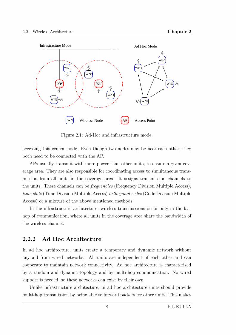
Figure 2.1: Ad-Hoc and infrastructure mode.
accessing this central node. Even though two nodes may be near each other, they
both need to be connected with the AP.
APs usually transmit with more power than other units, to ensure a given cov-
erage area. They are also responsible for coordinating access to simultaneous trans-
mission from all units in the coverage area. It assigns transmission channels to
the units. These channels can be frequencies (Frequency Division Multiple Access),
time slots (Time Division Multiple Access) orthogonal codes (Code Division Multiple
Access) or a mixture of the above mentioned methods.
In the infrastructure architecture, wireless transmissions occur only in the last
hop of communication, where all units in the coverage area share the bandwidth of
the wireless channel.
2.2.2 Ad Hoc Architecture
In ad hoc architecture, units create a temporary and dynamic network without
any aid from wired networks. All units are independent of each other and can
cooperate to maintain network connectivity. Ad hoc architecture is characterized
by a random and dynamic topology and by multi-hop communication. No wired
support is needed, so these networks can exist by their own.
Unlike infrastructure architecture, in ad hoc architecture units should provide
multi-hop transmission by being able to forward packets for other units. This makes
8 Elis KULLA
2.3. Wireless vs. Wired Chapter 2
the units operate in both end device mode as well as router mode. The MANET
work group of IETF is formed to support Ad hoc issues and improvements.
In Fig. 2.1, in infrastructure architecture of a 802.11b, even though their trans-
mission range cover each other geographical position, nodes WN1 and WN3 are part
of different infrastructures, separated by APs. Thus, they can communicate only
through their respective APs. While, in Ad hoc mode, each node can communicate
with every other node which is inside its transmission range. This means that Ad
Hoc Networks do not need the aid of any central device. By avoiding the centralized
administration of the network in ad hoc infrastructure, the “one point of failure” is
also avoided.
2.3 Wireless vs. Wired
The evolution from wired networks to wireless networks has lead to some issues due
to some problem-posing phenomena. These phenomena, should be addressed cor-
rectly, when deploying the communication algorithm. Three of the most problematic
phenomena are discussed in following.
2.3.1 Collision
When two units in the same network try to communicate simultaneously in the
same channel, collision occurs. In wired networks, switching devices are used to
allow units to take turns sending packets, while in wireless networks communication
is done through an antenna, which usually is omni-directional. This makes it more
difficult to control the collision issue, because a single antenna can be used only for
receiving or only for transmitting in a certain given time. Thus, if two units try
to transmit messages to the same third party unit, this unit will not understand
neither of the messages.
2.3.2 Unidirectional Links
In wired networks a link is always available from both sides communicating, being a
two-way link. While, in wireless networks this situation is not always true. The units
may have different antenna characteristics, the receiving and transmitting circiuts
may provide different power levels, and there may be interference from other sources.
9 Elis KULLA
2.4. The Wireless Channel Chapter 2
These conditions cause some links to be unidirectional, being one-way links. This
means a unit should be aware of the availability of both direction links, before
transmitting any signal.
2.3.3 Asymmetric Links
Another phenomena which may occur due to radio irregularities, is the asymmetric
links. An asymmetric link has different network parameters for downstreaming and
upstreaming (like an ADSL line). These links may cause problems if not taken into
account by the communicating units.
2.4 The Wireless Channel
Communication of nodes in Ad Hoc Networks are done through wireless transceivers.
Thus, the wireless channel is an important block of any model used to describe a
wireless system. A more detailed description can be found in [28].
A radio channel between a transmitter unit u and a receiver unit v is established
if and only if the power of the radio signal received by node v is above the sensitivity
threshold. Theoretically, there exists a direct wireless link between a transmitter
unit u and a receiver unit v if Pr ≥ β, where Pr is the power of the signal received
by v, and β denotes the sensitivity threshold. The exact value of β depends on
the features of the wireless transceiver and on the communication data rate. If
we increase the data rate for a given radio, the value of β will be increased. The
received power Pr is affected by the power Pt used by unit u to transmit, and on
the path loss, which models the wireless signal degradation with distance. Denoting
with PL(u, v) the path loss between units u and v, we can write:
Pr =Pt
PL(u, v). (2.1)
Modeling path loss is one of the most difficult tasks of the wireless system designer.
The mechanisms that affect the radio signal propagation can be classified into three
major categories: reflection, diffraction and scattering.
• When electromagnetic waves hit the surface of a large object (earth surface,
large buildings etc.), compared to the wavelength of the propagating signal,
reflection occurs.
10 Elis KULLA
2.4. The Wireless Channel Chapter 2
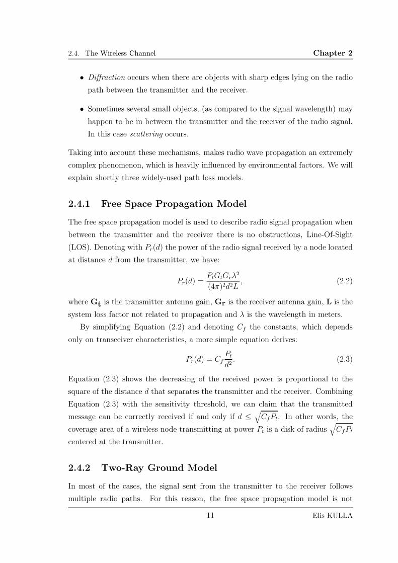
• Diffraction occurs when there are objects with sharp edges lying on the radio
path between the transmitter and the receiver.
• Sometimes several small objects, (as compared to the signal wavelength) may
happen to be in between the transmitter and the receiver of the radio signal.
In this case scattering occurs.
Taking into account these mechanisms, makes radio wave propagation an extremely
complex phenomenon, which is heavily influenced by environmental factors. We will
explain shortly three widely-used path loss models.
2.4.1 Free Space Propagation Model
The free space propagation model is used to describe radio signal propagation when
between the transmitter and the receiver there is no obstructions, Line-Of-Sight
(LOS). Denoting with Pr(d) the power of the radio signal received by a node located
at distance d from the transmitter, we have:
Pr(d) =PtGtGrλ
2
(4π)2d2L, (2.2)
where Gt is the transmitter antenna gain, Gr is the receiver antenna gain, L is the
system loss factor not related to propagation and λ is the wavelength in meters.
By simplifying Equation (2.2) and denoting Cf the constants, which depends
only on transceiver characteristics, a more simple equation derives:
Pr(d) = Cf
Pt
d2. (2.3)
Equation (2.3) shows the decreasing of the received power is proportional to the
square of the distance d that separates the transmitter and the receiver. Combining
Equation (2.3) with the sensitivity threshold, we can claim that the transmitted
message can be correctly received if and only if d ≤√
CfPt. In other words, the
coverage area of a wireless node transmitting at power Pt is a disk of radius√
CfPt
centered at the transmitter.
2.4.2 Two-Ray Ground Model
In most of the cases, the signal sent from the transmitter to the receiver follows
multiple radio paths. For this reason, the free space propagation model is not
11 Elis KULLA
2.4. The Wireless Channel Chapter 2
Direct Path
Ground Reflected Path
Node u
Node v
ht
hr
d
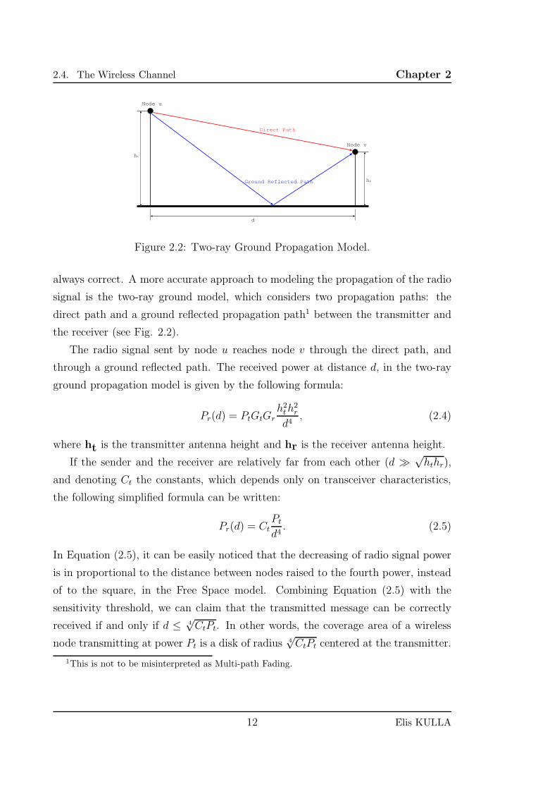
Figure 2.2: Two-ray Ground Propagation Model.
always correct. A more accurate approach to modeling the propagation of the radio
signal is the two-ray ground model, which considers two propagation paths: the
direct path and a ground reflected propagation path1 between the transmitter and
the receiver (see Fig. 2.2).
The radio signal sent by node u reaches node v through the direct path, and
through a ground reflected path. The received power at distance d, in the two-ray
ground propagation model is given by the following formula:
Pr(d) = PtGtGr
h2th
2r
d4, (2.4)
where ht is the transmitter antenna height and hr is the receiver antenna height.
If the sender and the receiver are relatively far from each other (d ≫√hthr),
and denoting Ct the constants, which depends only on transceiver characteristics,
the following simplified formula can be written:
Pr(d) = Ct
Pt
d4. (2.5)
In Equation (2.5), it can be easily noticed that the decreasing of radio signal power
is in proportional to the distance between nodes raised to the fourth power, instead
of to the square, in the Free Space model. Combining Equation (2.5) with the
sensitivity threshold, we can claim that the transmitted message can be correctly
received if and only if d ≤ 4√CtPt. In other words, the coverage area of a wireless
node transmitting at power Pt is a disk of radius 4√CtPt centered at the transmitter.
1This is not to be misinterpreted as Multi-path Fading.
12 Elis KULLA
2.5. Wireless Technologies Chapter 2
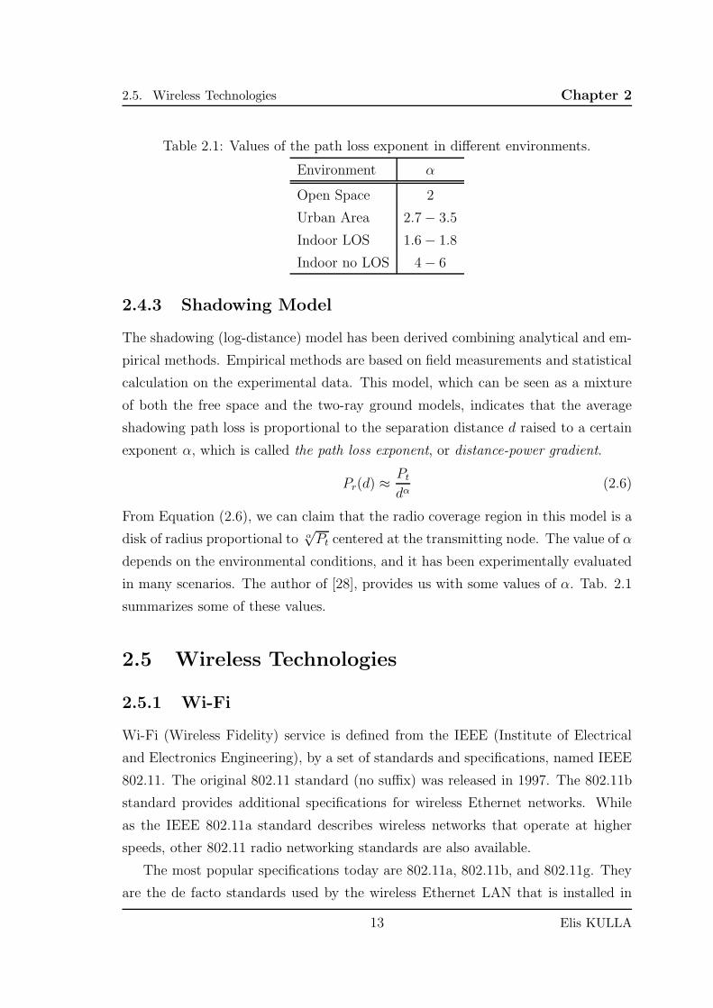
Table 2.1: Values of the path loss exponent in different environments.
Environment α
Open Space 2
Urban Area 2.7− 3.5
Indoor LOS 1.6− 1.8
Indoor no LOS 4− 6
2.4.3 Shadowing Model
The shadowing (log-distance) model has been derived combining analytical and em-
pirical methods. Empirical methods are based on field measurements and statistical
calculation on the experimental data. This model, which can be seen as a mixture
of both the free space and the two-ray ground models, indicates that the average
shadowing path loss is proportional to the separation distance d raised to a certain
exponent α, which is called the path loss exponent, or distance-power gradient.
Pr(d) ≈Pt
dα(2.6)
From Equation (2.6), we can claim that the radio coverage region in this model is a
disk of radius proportional to α
√Pt centered at the transmitting node. The value of α
depends on the environmental conditions, and it has been experimentally evaluated
in many scenarios. The author of [28], provides us with some values of α. Tab. 2.1
summarizes some of these values.
2.5 Wireless Technologies
2.5.1 Wi-Fi
Wi-Fi (Wireless Fidelity) service is defined from the IEEE (Institute of Electrical
and Electronics Engineering), by a set of standards and specifications, named IEEE
802.11. The original 802.11 standard (no suffix) was released in 1997. The 802.11b
standard provides additional specifications for wireless Ethernet networks. While
as the IEEE 802.11a standard describes wireless networks that operate at higher
speeds, other 802.11 radio networking standards are also available.
The most popular specifications today are 802.11a, 802.11b, and 802.11g. They
are the de facto standards used by the wireless Ethernet LAN that is installed in
13 Elis KULLA
2.5. Wireless Technologies Chapter 2
offices, on campus and in most home networks. The 802.11n standard will replace
both 802.11b and 802.11g. It is faster, more secure, and more reliable. The older
standards will still be supported, by the new Wi-Fi equipment.
2.5.2 WiMAX
Worldwide Interoperability for Microwave Access (WiMAX) is a metropolitan area
network service that usually uses base stations which can provide service to users
within a 30-mile radius. WiMAX service providers use licensed operating frequencies
between 2 GHz and 11 GHz in which a WiMAX link can transfer data at up to
70Mbps. When many users share a single WiMAX tower and base station, the signal
quality deteriorates. WiMAX is an independent radio system that is designed to
either supplement or replace the existing broadband Internet distribution systems.
In practice, WiMAX competes with both 3G wireless services and with Internet
service providers that distribute Internet access to fixed locations through telephone
lines and cable television utilities. Subscribers to aWiMAX service usually use either
a wired LAN or Wi-Fi to distribute the network within their buildings.
2.5.3 Bluetooth
Bluetooth uses radio signals to replace the wires and cables that connect a computer
or a mobile telephone to peripheral devices, such as a keyboard, a mouse, or a set
of speakers. The Bluetooth can also be used to transfer data between a computer
and a mobile telephone, smartphone, BlackBerry, or other PDAs (Personal Digital
Assistant). Bluetooth moves among 79 different frequencies 1,600 times per second
in the same unlicensed 2.4 GHz range as 802.11b and 802.11g Wi-Fi services. Blue-
tooth is not very practical for connecting a computer to the Internet because it’s
slow (the maximum data transfer rate is only about 3Mbps), and it has a very lim-
ited signal range (maximum 100 meters with LOS). In order to prevent interference
between Bluetooth and Wi-Fi signals, many computers that use both technologies
(including the widely used Intel Centrino chip set) coordinate the two services. This
coordinated operation is slightly slower than either service operating alone, but the
difference is insignificant.
14 Elis KULLA
2.5. Wireless Technologies Chapter 2
2.5.4 4G Cellular Networks
4G is being developed to accommodate the QoS and rate requirements set by further
development of existing 3G applications like WBA, Multimedia Messaging Service
(MMS), video chat, mobile TV, but also new services like HDTV content, minimal
services like voice and data, and other services that utilize bandwidth. It may be
allowed roaming with WLANs, and be combined with digital video broadcasting
systems.
According to the members of the 4G working group, the infrastructure and the
terminals of 4G will have almost all the standards from 2G to 4G implemented.
Although legacy systems are in place to adopt existing users, the infrastructure
for 4G will be only packet-based (all-IP). Some proposals suggest having an open
Internet platform. Technologies considered to be early 4G include: Flash-OFDM,
the 802.16e mobile version of WiMax, and HC-SDMA.
2.5.5 MANETs
The rapid deployment of a mobile user, is going to be present in the next gen-
eration of wireless systems. Some real applications include establishing survivable,
dynamic communication for emergency/rescue operations, disaster relief efforts, and
military networks. Such network scenarios cannot rely on centralized and organized
connectivity.
A MANET is an autonomous group of mobile terminals that communicate with
each other over wireless links. Thee network topology may change quickly and
randomly over time, because terminals are mobile. The network is decentralized,
and all network activity such as, discovering the topology and delivering messages
must be executed by the nodes themselves. For this reason, routing functionality
will be incorporated into these mobile nodes.
The set of applications for MANETs is wide, ranging from small, static networks
to large, highly dynamic networks. Designing the protocols for these networks, in
order to determine network organization, link scheduling, and routing is a very com-
plex issue. However, determining viable routing paths and delivering messages in a
decentralized environment where network topology fluctuates is not a well-defined
problem. While the shortest path (based on a given cost function) from a source to
a destination in a static network is usually the optimal route, this idea is not easily
15 Elis KULLA
2.5. Wireless Technologies Chapter 2
extended to MANETs. Factors such as variable wireless link quality, propagation
path loss, multiuser interference, power expended, and topological changes, are rel-
evant issues. The network should be able to adaptively alter the routing paths to
alleviate any of these effects.
16 Elis KULLA
Chapter 3
MANET
MANETs are formed by several wireless terminals, which can be mobile or semi-
mobile. These terminals, or nodes, do not have a pre-established infrastructure,
meaning that they create a fast and temporary network whenever they are deployed
in an environment. Each of the nodes has a wireless interface and communicate with
each other over radio or infrared links in a Peer-to-Peer (P2P) design. Examples of
MANET nodes are, notebooks and PDAs used widely now everywhere. In general,
nodes in MANETs are mobile, and their movement is random and difficult to be
modeled, but according to mankind lifestyle, we always try to implement similar
models to what happens in real life. Some nodes can be static as well. they can be
used to interconnect the Ad Hoc Network to another network or the Internet, or the
user simply is sitting with his notebook and using network resources.
MANETs need to have implemented some mechanisms as follows.
• If provides inter-networking, an Internet access mechanisms is needed.
• Self configuring networks requires an address allocation mechanism.
• Mechanism to detect and act on merging of existing networks.
• Security mechanisms.
• Nodes must be able to relay traffic since communicating nodes might be out
of range.
• Multi-hop operation requires a routing mechanism designed for mobile nodes.
17
3.1. MANETs Usage and Applications Chapter 3
3.1 MANETs Usage and Applications
Recently, MANETs have drawn too much attention as a research field. As a result of
this considerable research activity, the basic mechanisms that enable wireless ad hoc
communication have been designed and standardized. The future seems to be bright
for MANETs, which will take advantage of its most distinguishable characteristics,
mobility and multi-hop, to take the place of wired multi-hop backbones, because they
are so easy and inexpensive to be implemented, even in areas where infrastructure
is impossible to appear.
MANETs are the networks of the future in many applications. By using ad hoc
philosophy, each user (node) gets in and out of the network whenever it finds it
convenient, without being noticed by other users. This means, that even in the
worst case of an unexpected failure of a node, the network is still up. This brings
a lot of advantages in using MANETs in many applications. Some of the most
common application fields, in which MANETs have great success are:
Military Scenarios : In battlefield it is preferable to make a very quick deploy-
ment of information networks, and without the use of any infrastructure or
centralized administration.
Sensor Networks : WSNs are a very interesting application of MANETs, where
a bunch of sensors, equipped with a radio antenna, are able to send useful
collected information to where we want, or compute aggregate values of the
parameters sensed in the environment.
Students Campus : That is a very useful application, for every environment
where density of wireless terminals is high enough to cover the intended area.
Conferences : The property of quick-deployment and mobility, make MANETs an
adaptive tool to keep everyone connected in the conferences.
OLPC : One Laptop Per Child project [29] is being implemented in developing
countries, where sometimes there is no proper infrastructure for all laptops to
stay connected. MANETs provide the solution here.
18 Elis KULLA
3.2. MANETs Challenges Chapter 3
3.2 MANETs Challenges
Even though the technology for MANETs exists and is developing, applications
based on the ad hoc networking paradigm are almost completely lacking. This is
because many of the challenges to be faced for a practical implementation of ad hoc
network services are still to be solved.
Energy Conservation: Units in MANETs are typically battery equipped. One of
the primary design goals is to use limited amount of energy as efficiently as
possible.
Unstructured and Changeable Network Topology: Since the network nodes
can, in principle, be arbitrarily placed in a certain region and are typically
mobile, the topology of the graph that represents the wireless communication
links between the nodes is usually unstructured. Furthermore, the network
topology may vary with time, because of node mobility or failure. In these
conditions, optimizing the performance of ad hoc network protocols is a very
difficult task.
Low-quality Communications: Communication on a wireless channel is, in gen-
eral, much less reliable than in a wired channel. Furthermore, the quality
of communication is influenced by environmental factors (weather conditions,
presence of obstacles, interference with other radio networks, etc.), which are
time varying. Thus, applications for MANETs should be resilient to dramat-
ically varying link conditions, tolerating also non-negligible off-service time
intervals of the wireless link.
Resource-constrained Computation: MANETs are characterized by low resource
availability. In particular, energy and network bandwidth are available in very
limited amounts as compared to more traditional network paradigms. Proto-
cols for MANETs must strive to provide the desired performance level in spite
of the few available resources.
Scalability: In some MANET scenarios, the network can be composed of hundreds
or of nodes. This means that protocols for MANETs must be able to operate
efficiently in the presence of a very large number of nodes also.
19 Elis KULLA
3.3. Routing in MANETs Chapter 3
In case of MANETs used for “ubiquitous” networking, the following issues must also
be addressed.
Interoperability: In the “ubiquitous” networking scenario data can travel through
the most diverse type of networks: ad hoc, cellular, satellite, wireless LAN,
PSTN, Internet, and so on. Ideally, the user should smoothly switch from one
network to the other without interrupting his applications. Implementing this
sort of ’network handoff’ is a very challenging task.
Definition of Feasible Business Models: Today, accounting in wireless networks
(cellular, and commercial wireless Internet access) is done at the base station,
that is, using a centralized infrastructure. Furthermore, roaming is allowed
only within networks of the same type (e.g. cell phone roaming when the
user is in a foreign country). In the ubiquitous scenario, it is still not clear
which infrastructure should perform billing and which rules should be used to
regulate roaming between different types of networks.
Stimulate Cooperation Between Nodes: When designing a certain network pro-
tocol, it is usually assumed that all the nodes in the network voluntarily par-
ticipate in the protocol execution. In some MANET application scenarios,
network nodes are owned by different authorities (private users, professionals,
profit and/or nonprofit organizations, and so on), and voluntary participation
in the protocol execution cannot be taken for granted. Thus, network nodes
must be somehow stimulated to behave according to the protocol specifica-
tions.
3.3 Routing in MANETs
There are many reasons why mobile ad hoc networking is being researched by many
organizations and institutes around the globe. The dynamic nature and the lack
of infrastructure of these networks, is asking more and more implementation of
networking strategies and paradigms, to be able to provide efficient communication.
Along with that, the variety of applications of MANETs in different scenarios, have
made research interests growing in this field.
In MANETs, the well-known TCP/IP structure is used by the nodes to make
the communication happen. However, due to their mobility and low resource ca-
20 Elis KULLA
3.3. Routing in MANETs Chapter 3
pacities, for the MANETs to function efficiently, one should modify each layer of
TCP/IP stack. Thus, many routing protocols and algorithms are developed and
proposed, and each author of each of the protocols, claims improvements over ex-
isting approaches, for specific network scenarios. For a routing protocol to function
efficiently in MANETs, it should have the following features:
• Self starting and self organizing,
• Multi-hop, loop-free paths,
• Dynamic topology maintenance,
• Rapid convergence,
• Minimal network traffic overhead,
• Scalable to large networks.
The routing protocols are separated into two main categories:
1. Reactive MANET Routing Protocols (RMRP).
2. Proactive MANET Routing Protocols (PMRP).
Adaptive or Hybrid Routing Protocols are also available, but these protocols use
features of both RMRP and PMRP, mixed together. In this section, we give a short
description of routing protocol categories, some routing protocols for each category
and some features of each. A review of these routing protocols when used in large
scalable MANETs can be found in [30].
3.3.1 Proactive Routing
Proactive routing protocols function in a way that each node maintains routing
information to every other node (or nodes located in a specific part) in the network,
in one or many tables or lists. This means that all routes are maintained during all
the time of network operation. Topology changes, which is very frequent in MANETs
brings a lot of traffic control information exchanged between nodes. PMRPs differ
among each other in the way each node updates and detects the routing information,
and the number of tables used to keep different types of information. Although
the routes in PMRPs are always available, constant overhead is created by control
21 Elis KULLA
3.3. Routing in MANETs Chapter 3
traffic. Some of the most popular PMRPs are: Destination Sequenced Distance
Vector (DSDV), Fisheye State Routing (FSR) and Optimized Link State Routing
(OLSR). We will present OLSR and BATMAN protocols in following.
3.3.1.1 Optimized Link State Routing (RFC3626)
The OLSR protocol for mobile ad hoc networks is a PMRP. It is developed as a
MANET compatible version of the classical link state algorithm. OLSR source code
is available online, and it can be found in http://www.olsr.org. The new concept
OLSR brought to MANET, is MultiPoint Relaying (MPR). Lets explain in short
details the functioning of OLSR. The OLSR protocol can be divided in to three
main modules:
• Neighbor/link sensing,
• Optimized flooding/forwarding (MPR),
• Link-State messaging and route calculation.
Neighbor and link sensing is realized by sending HELLO packets. All nodes trans-
mit HELLO packets at a given interval. The 3-way handshake performed by two
neighbors creates link information for both nodes. The HELLO packets also contain
information about all active neighbors, so each node knows about 1-hop and 2-hop
neighbors. Topology Control (TC) packets are also exchanged between neighbors to
keep track of topology changing.
If OLSR would make a regular flooding of HELLO packets, too much unwanted
traffic would flow on the network. The optimization of OLSR consists on exactly
decreasing this traffic overhead. This is done by introducing the new concept of
MPR. Node X choses a set mpr(X) of MPRs from its 1-hop neighbors, so that all
2-hop neoghbors of node X is reached via the set mpr(X). Flooding and forwarding
is thus optimized in this way. A node recieveing a packet from node X, forwards or
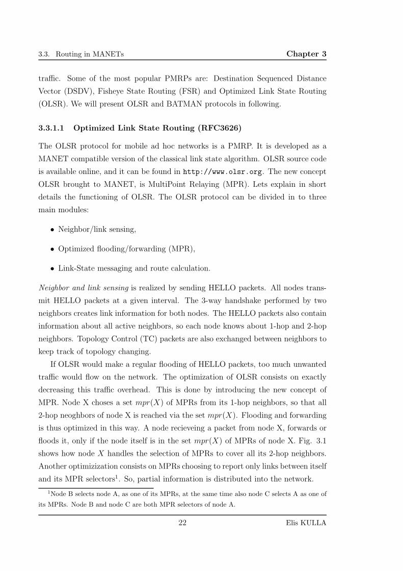
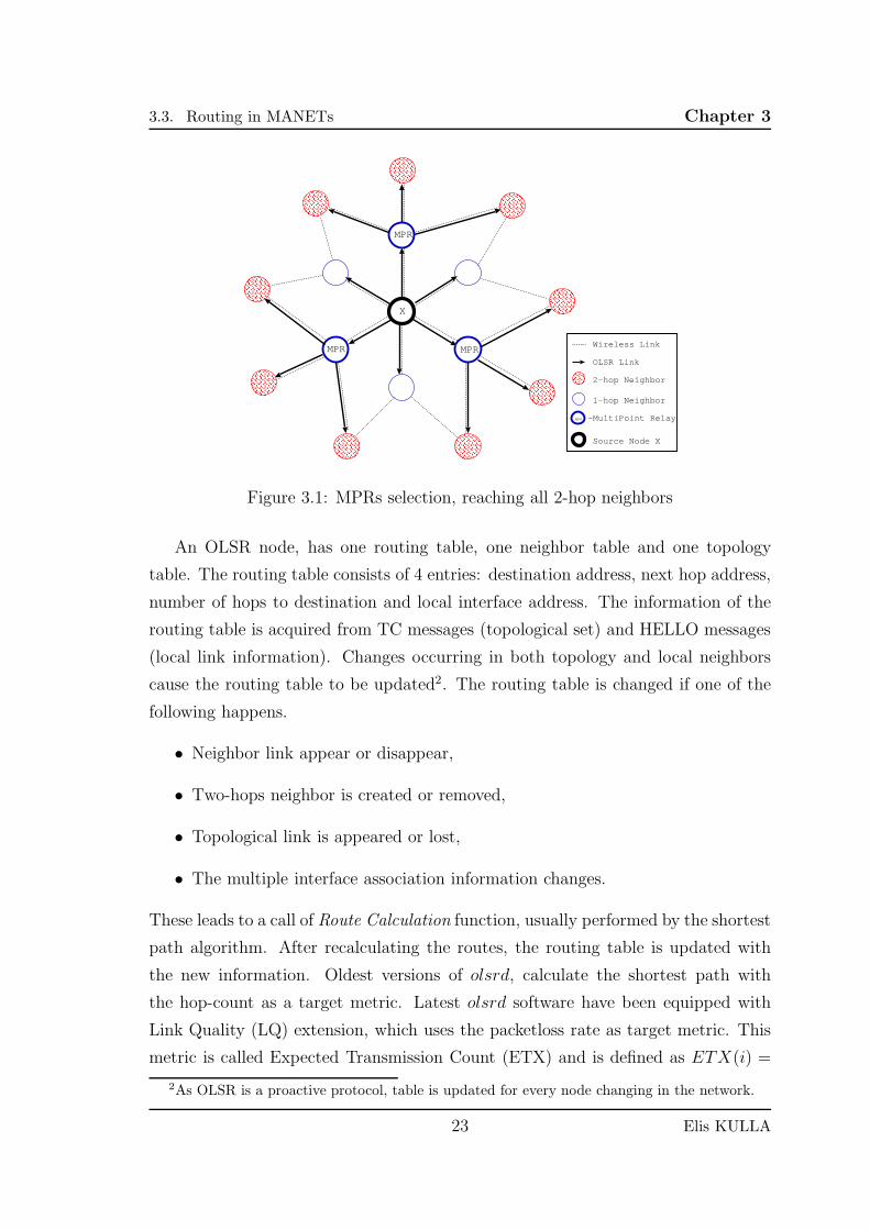
floods it, only if the node itself is in the set mpr(X) of MPRs of node X. Fig. 3.1
shows how node X handles the selection of MPRs to cover all its 2-hop neighbors.
Another optimizization consists on MPRs choosing to report only links between itself
and its MPR selectors1. So, partial information is distributed into the network.
1Node B selects node A, as one of its MPRs, at the same time also node C selects A as one of
its MPRs. Node B and node C are both MPR selectors of node A.
22 Elis KULLA
3.3. Routing in MANETs Chapter 3
Wireless Link
OLSR Link
2-hop Neighbor
1-hop Neighbor
Source Node X
X
MPR
MPRMPR
-MultiPoint RelayMPR
Figure 3.1: MPRs selection, reaching all 2-hop neighbors
An OLSR node, has one routing table, one neighbor table and one topology
table. The routing table consists of 4 entries: destination address, next hop address,
number of hops to destination and local interface address. The information of the
routing table is acquired from TC messages (topological set) and HELLO messages
(local link information). Changes occurring in both topology and local neighbors
cause the routing table to be updated2. The routing table is changed if one of the
following happens.
• Neighbor link appear or disappear,
• Two-hops neighbor is created or removed,
• Topological link is appeared or lost,
• The multiple interface association information changes.
These leads to a call of Route Calculation function, usually performed by the shortest
path algorithm. After recalculating the routes, the routing table is updated with
the new information. Oldest versions of olsrd, calculate the shortest path with
the hop-count as a target metric. Latest olsrd software have been equipped with
Link Quality (LQ) extension, which uses the packetloss rate as target metric. This
metric is called Expected Transmission Count (ETX) and is defined as ETX(i) =
2As OLSR is a proactive protocol, table is updated for every node changing in the network.
23 Elis KULLA
3.3. Routing in MANETs Chapter 3
1/(NI(i) ∗ LQI(i)), where NI(i) is the packet arrival rate seen by a node on the
i-th link during the window W and LQI(i) is the estimation of the packet arrival
rate seen by its neighbor on the same link. This LQ extension enhances the packet
delivery ratio in comparison with the old technique. Authors in [31] have found the
optimal value of LQWS (Link Quality Window Size) for TCP flow, to be exactly
10. In [32] can be found the RFC3626 document for more detailed descriptions.
Anyway, the OLSR protocol is not implemented in practical scenarios. Routing
tables taking a long time to build, routing loops and flapping routes are some of
several issues that OLSR shows. A new routing protocol started to be developed, in
order to overcome these issues. This new protocol will be described in the following.
3.3.1.2 Better Approach To MANET (BATMAN)
BATMAN is introduced as a better approach to solve these issues of OLSR. In BAT-
MAN there is no dissemination of topology. Nodes execute the following operations:
1. Send periodic messages, called OGMs (OriGinator Messages). These OGMs
contain 4 fields of data: the IP address of the originator, the IP address of the
forwarding node, a TTL value and a sequence number (SQ), consisting of 52
bytes, in total.
2. Check the best one-hop neighbor for every destination in the network, by
building a ranking table.
3. Rebroadcast the OGMs received from the best one-hop neighbor, or from the
originator itself.
The timer in BATMAN is used for sending OGMs. The bi-directionality of links
is checked using the SQ of OGM. If the SQ of and OGM received from a particular
node falls within a certain range, the corresponding link is considered bi-directional.
For example, suppose that in a time interval T , the node A sends Tr messages,
where Tr is the rate of OGM messages. The neighbors of A will re-broadcast the
OGMs of A and also other node’s OGMs. When A receives some OGMs from
a neighbor node B, if the last received OGM from B has a SQ less or equal to
Tr, then B is considered bi-directional, otherwise it is considered unidirectional.
Bi-directional links are used for the ranking procedure. The quantity Tr is called
bidirectional sequence number range. The ranking procedure is the same as the link
24 Elis KULLA
3.3. Routing in MANETs Chapter 3
quality extension of OLSR. In few words, every node ranks its neighboring nodes by
counting the total received OGMs from them. The ranking procedure is performed
on OriGinator (OG) basis. Initially, for every OG, every node stores a variable
called Neighbor Ranking Sequence Frame (NBRF), which is upper bounded by a
particular value called ranking sequence number range. Whenever a new OGM is
being received via a bi-directional link, the receiving node executes the following
steps.
1. If the sequence number of the OGM is less than the corresponding NBRF,
then drop the packet.
2. Otherwise, update the NBRF = SQ(OGM) in the rank table.
3. If SQ(OGM) is received for the first time, store OGM in a new row of the
rank table.
4. Otherwise, increment by one the OGM count or make ranking for this OGM.
Finally, the ranking procedures select as the best one-hop neighbor the one which has
the highest rank in the ranking table. This feature eliminates routing loops because
no global topology information are flooded, the self-interference due to data traffic
can cause oscillations in the throughput as we will see in our experiments. Let us
note that the same OGM packet is used for: link sensing, neighbor discovery, bi-
directional link validation and flooding mechanism. Other details on BATMAN can
be found in [33, 34]
3.3.2 Reactive Routing
In contrary with PMRPs, in RMRPs, routes are determined and maintained each
time nodes require them to send data to a destination. In this category of routing
protocols, the main control overhead is the route discovery traffic. Route discovery
is done by flooding a route request packet in the network. When destination (or
some node which has information about destination) is reached, a route reply packet
is sent back via link reversal, or via flooding to probably find a better route. Reac-
tive protocols can be classified into two categories: hop-by-hop routing and source
routing.
In Hop-by-hop Routing, data packet headers consist only of the destination ad-
dress and the next hop address. Thus, data packets are routed independently by
25 Elis KULLA
3.3. Routing in MANETs Chapter 3
each node, based on local information, making routes adaptable to dynamically
changing topology in MANETs. In this strategy, each node should have to main-
tain information about all active routes, and stay updated with all its neighbors.
Although this is a disadvantage in MANETs, in this scenario topology information
is fresher so we have better routes.
In Source Routed on-demand protocols each data packet is told the complete
route from source to destination. Intermediate nodes, route these packets according
to the information kept in the header of each packet. Thus, they do not need to
maintain fresh routing information for each active route. They also do not need to
maintain neighbor connectivity. In large networks source routing protocols do not
scale well due to the added route overhead by bigger headers, and the increase of
route failure probability (more nodes in a route).
RMRPs are designed to lower the overhead in proactive ones. Thus the main
advantage of reactive routing is that, the bandwidth is used only when needed to
find a route. The process of finding a route starts with a flooding and this usually
brings initial delays. Its worth to mention some well-known RMRPs: Ad hoc On-
demand Distance Vector (AODV), Dynamic Source Routing (DSR) and Temporally
Ordered Routing Algorithm (TORA). We will describe AODV in following.
3.3.2.1 Ad hoc On-Demand Distance Vector (RFC 3561)
AODV is one of the most popular reactive routing protocol for MANETs. Lets see
how this routing protocols works in a general view. For most detailed description
see [35].
As a reactive (on demand) protocol, when a node wants to transmit data, it
first starts a route discovery process, by flooding a RREQ (Route Request) packet.
The RREQ packet are forwarded by all the nodes by which it is received, until
the destination is found. On the way to destination, the RREQ informs all the
intermediate nodes about a route to the source. When the RREQ reaches the des-
tination, destination sends a Route Reply (RREP) packet which follows the reverse
path discovered by RREQ. This informs all intermediate nodes about a route to the
destination node. After RREQ and RREP are delivered to their destination, each
intermediate node on the route knows what node to forward data packets in order
to reach source or destination. Thus data packets do not need to carry addresses
26 Elis KULLA
3.4. MANET Research Tools Chapter 3
of all intermediate nodes in the route. It just carries the address of the destination
node, decreasing noticeably routing overheads.
A third kind of routing message, called route error (RERR), allows nodes to
notify errors, for example, because a previous neighbor has moved and is no longer
reachable. If the route is not active (i.e., there is no data traffic flowing through
it), all routing information expires after a timeout and is removed from the routing
table.
AODV is based on DSDV and DSR algorithms. The best advantage to DSR
and DSDV is that in AODV, packets being sent (the RREP packet also) carry
only the address of the destination and not the addresses of all the intermediate
nodes to make the delivery. This lowers routing overheads. In AODV the route
discovery process may last for a long time, or it can be repeated several times, due
to potential failures during the process. This introduces extra delays, and consumes
more bandwidth as the size of the network increases.
3.3.3 Adaptive and Hybrid Routing Protocols
Proactive and reactive routing protocols have both its pros and cons. Thinking to get
the best possible approach for a routing strategy, hybrid routing protocols appeared
as trying to use the best features of both proactive and reactive. These protocols
are designed to be scalable to large network. The whole network is separated in
hierarchical regions, usually geographical. Some nodes are grouped trees, some
trees or clusters, some clusters are grouped in a domain, and so on. Nodes within
a region stay updated proactively, while to send data to a node in another region,
route discovery process starts reactively. This strategy, lowers the route discovery
overhead and supports very good scalability to larger networks.
3.4 MANET Research Tools
A collection of wireless mobile hosts that can dynamically establish a temporary
network without any aid from fixed infrastructure is known as a MANET. These
hosts can move in different directions with different speeds. MANET are found
very useful in real applications such as time-lacking implementations and indoor
environments.
27 Elis KULLA
3.4. MANET Research Tools Chapter 3
A lot of research for MANETs has been done in simulation, because in general,
a simulator can give a quick and inexpensive evaluation of protocols and algorithms.
Emulation also is a good tool for research in MANETs. Hardware and simulation
software components are mixed together, to create an emulation system. However,
experimentation in the real world are very important to verify the simulation or
emulation results and to revise the models implemented.
One of the most discussed models in literature is the mobility model. There are a
lot of mobility models, which can be used in simulations and emulations, for testing
MANETs. On the other hand, mobility models for real world experiments are more
complicated as they require more cost, more time and/or more people. They can be
implemented by people carrying nodes and walking around, or cars driving around,
or even robots. In this chapter, we will make a survey on MANETs testbeds and
how they implement mobility model.
3.4.1 Evaluation Techniques
In a research environment, research tools are required to test, verify and identify
problems of an algorithm or protocol. These tools are classified in three major
techniques: simulators, emulators and real-world testbeds. We will describe them
shortly in the following.
3.4.1.1 Simulations
A simulation system consists of many assumptions and artificial modeling, in order
to reach a certain realistic degree. However, these assumptions and modeling can
have errors and in some cases, some realistic effects are not even considered, e.g.
gray zones effect [1] are not considered in the well-known simulator ns-2. In the
early phases of the development of a MANET algorithm or protocol, usually after
the analytical modeling, simulations can give a quick and inexpensive result regard-
ing the theoretical performance. Moreover, we can keep unchanged the simulated
conditions and parameters and run the simulations as many times as we want.
3.4.1.2 Emulators
With a higher degree of realism than simulators, emulators can still control the
repeatability of tests and use real hardware combined with simulation software, to
conduct experiments in controlled conditions. They use artificial assumptions which
28 Elis KULLA
3.4. MANET Research Tools Chapter 3
are sometimes unrealistic. Emulators can be divided into physical layer emulators
and MAC layer emulators. Physical layer emulators, e.g. EWANT [36], use the
attenuation of the radio signal to emulate movement or obstacles. MAC layer em-
ulators use MAC filter tools, e.g. Dummynet [37], to decide network topology and
emulate mobility. Emulators have higher costs than simulators because they use
real hardware.
3.4.1.3 Real-World Testbeds
Real-world testbeds have the higher level of realism because they are not based
on assumptions about the experimental conditions. In testbeds, when mobility
is present, the node changes its geographical location, which can have different
effects on the performance. Testbeds are usually used on the final stages of the
development of an algorithm or protocol. Simulation and emulation systems can
make assumptions based on experimental results provided by testbeds. However,
real-world testbed implementations have higher costs for hardware software and
working hours. Also, the repeatability of tests in a testbed is a complicated and
costly task.
3.4.2 Mobility in MANETs
With the growing applications, services and technologies of the Internet, nowadays
users apart from using wireless devices, most of them are on the move for most
of time. Also in MANET, Wireless Sensor Networks (WSNs) or Vehicular Adhoc
Networks (VANETs), mobility is a very important feature. When it comes to testing
these networks, using the tools explained in Section 3.4.1, a researcher chooses the
pattern of movement of the nodes during the evaluation time. This pattern is defined
as a mobility model, and in simulations there are a lot of mobility models proposed
and used. In [38], the authors present a survey on mobility models and they classify
them in:
Entity Mobility Models: All nodes move independently from each other.
Group Mobility Models: Nodes movement is dependent from other nodes in the
network.
29 Elis KULLA
3.4. MANET Research Tools Chapter 3
Mobility models in reality derive logically from different aspects of life and we
can classify them in the following categories. A mobility pattern can be a mixing of
all of the following.
Biology Related Mobility Models: The movement of nodes are similar to real
biological species (insects, birds, fish, animals).
Activity Related Mobility Models: Different human activities, as sports, leisure
etc., create different mobility patterns.
Environment Related Mobility Models: The moving pattern in cities is dif-
ferent from that on an open field and highways. Mobility models driven by
environment are used a lot in research recently.
Random Mobility Models: These models are mostly used in simulations, when
mobility is not a specific requirement. Nodes choose random directions, ran-
dom destinations, random speed etc, moving in a specific area.
Considering a MANET testbed, the implementation of a mobility model is not a
simple task. We will discuss some experimental systems and the mobility they used
in the following section.
3.4.3 Real Testbeds with Mobility
Implementing mobility in a real-world testbed has encountered a lot of difficulties
and tasks. Recently there are a lot of testbeds running in universities or research
institutes. Some of them did not even consider mobility [39]. We show the charac-
teristics of the testbeds in Table 3.1 and will describe some of them in the following,
concentrating on the implementation of mobility.
In [40], the authors created a testbed for indoor and outdoor experimentations.
In indoor environment, they used horizontal and vertical topologies, and imple-
mented mobility by people carrying or pushing the wireless nodes. They used
AODV, OLSR and BATMAN routing protocols and measured performance by inves-
tigating many metrics. An interesting finding, which is different from what expected,
is that TCP transmission has a better performance than UDP transmission.
The authors of [13], introduce their APE testbed consisting of 37 nodes. Mobility
is implemented by people carrying laptops and walking around the testing indoor
and outdoor area, following the instructions on the screen. They conducted many
30 Elis KULLA
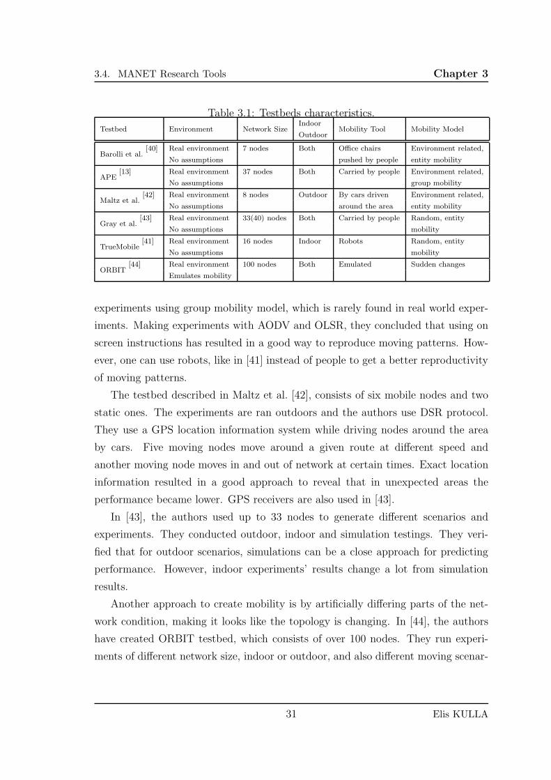
3.4. MANET Research Tools Chapter 3
Table 3.1: Testbeds characteristics.
Testbed Environment Network SizeIndoor
Mobility Tool Mobility ModelOutdoor
Barolli et al.[40] Real environment 7 nodes Both Office chairs Environment related,
No assumptions pushed by people entity mobility
APE[13] Real environment 37 nodes Both Carried by people Environment related,
No assumptions group mobility
Maltz et al.[42] Real environment 8 nodes Outdoor By cars driven Environment related,
No assumptions around the area entity mobility
Gray et al.[43] Real environment 33(40) nodes Both Carried by people Random, entity
No assumptions mobility
TrueMobile[41] Real environment 16 nodes Indoor Robots Random, entity
No assumptions mobility
ORBIT[44] Real environment 100 nodes Both Emulated Sudden changes
Emulates mobility
experiments using group mobility model, which is rarely found in real world exper-
iments. Making experiments with AODV and OLSR, they concluded that using on
screen instructions has resulted in a good way to reproduce moving patterns. How-
ever, one can use robots, like in [41] instead of people to get a better reproductivity
of moving patterns.
The testbed described in Maltz et al. [42], consists of six mobile nodes and two
static ones. The experiments are ran outdoors and the authors use DSR protocol.
They use a GPS location information system while driving nodes around the area
by cars. Five moving nodes move around a given route at different speed and
another moving node moves in and out of network at certain times. Exact location
information resulted in a good approach to reveal that in unexpected areas the
performance became lower. GPS receivers are also used in [43].
In [43], the authors used up to 33 nodes to generate different scenarios and
experiments. They conducted outdoor, indoor and simulation testings. They veri-
fied that for outdoor scenarios, simulations can be a close approach for predicting
performance. However, indoor experiments’ results change a lot from simulation
results.
Another approach to create mobility is by artificially differing parts of the net-
work condition, making it looks like the topology is changing. In [44], the authors
have created ORBIT testbed, which consists of over 100 nodes. They run experi-
ments of different network size, indoor or outdoor, and also different moving scenar-
31 Elis KULLA
3.4. MANET Research Tools Chapter 3
ios. Mobility is realized using MAC filtering techniques, redirecting traffic to other
nodes.
3.4.4 Discussion
Observing the experiences of testbed implementers, first of all we would like to
mention that, building a testbed with mobility needs hard work and endurance. We
did not talk about the beginning of implementation as it is not in the scope of our
work.
When planning to implement a mobility model in a testbed, the first important
thing that should be taken care about is what effects can this mobility pattern have
on other research or real applications. It can be an environment-related, activity-
related, entity or group mobility model. After deciding the moving pattern, the
next problem is how to make real devices move in your experimental area, in order
to be able to repeat the same movement. Driving cars [42], pushing chairs [40] or
even carrying devices and walking around following on-screen instructions [13] are
preferred ways of completing this task. Using automated movable robots is a more
efficient technique. However this has a higher cost on each robot used. Another
way of implementing mobility is emulation [44]. This method is cheaper but make
unrealistic assumptions, by changing topology conditions without physically moving
the nodes.
When nodes are mobile, we would like to check the position of every node at
a given time of the experiment, after some months or years to verify the results.
Some used methods consist of GPS receivers [42], security cameras [41], or using the
relative Radio Signal Strength (RSS) to compute the location of nodes.
The experiences of other testbed builders have have good insights on building
your own testbed. Another benefit we can get from the experiences of a testbed,
is the use of settings in our simulation systems. As proved in [13], a simulation
system can have similar results to outdoor experiments, which will help us verify
our conclusions.
In this paper, we described shortly the evaluation techniques of algorithms and
protocols. We also present an overview of mobility models and showed some real
testbeds with mobility, implemented in the world. We make some conclusions on
our work in the following.
32 Elis KULLA
3.4. MANET Research Tools Chapter 3
• When using people to make the movement of the nodes, the on-screen instruc-
tions are a good way to recreate the moving patterns. Robots, on the other
hand, are more precise, but the cost per node increases.
• Monitoring location and time synchronization is a difficult task, but it results
in finding unpredictable effects,when nodes are mobile. It can also be used for
future reference to the experiments.
• Simulation systems can give approximate results for experiments, while for
indoor environments there are unpredicted results. Thus, testbed experiments
give a lot of feedback to make assumptions regarding the simulation systems.
33 Elis KULLA

Chapter 4
Testbed Implementation and
Experimental Scenarios
4.1 Testbed Design and Implementation
4.1.1 Description
We conducted our experiments in the stairs environment in our five-floor depart-
mental building and in the outdoor bridges connecting our department building with
other buildings in our university. The testbed consists of five laptops. The machines
operate on Ubuntu Linux with kernel 2.6.28 suitably modified in order to support
the wireless cards. The lynksys wireless network cards (Model: WUSB54G ver.
4) are usb-based cards with an external antenna of 2dBi gain, transmitting power
of 16+/-1dBm and receiving sensitivity of -80dBm. We verified that the external
antenna improves the quality of the first hop link, which is the link connecting the
ad-hoc network. The driver can be downloaded from the web site [45, 46].
In our testbed, we have two systematic traffic sources we could not eliminate:
the control traffic and the other wireless APs interspersed within the campus. The
control traffic is due to the ssh program, which is used to remotely start and con-
trol the measurement software on the source node. The other traffic source brings
interferences occupying the available bandwidth, which is typical in an academic
scenario.
To generate the traffic between nodes, we used Distributed Internet Traffic Gen-
erator (D-ITG) software, which is an Open Source Traffic Generator [47]. With
35
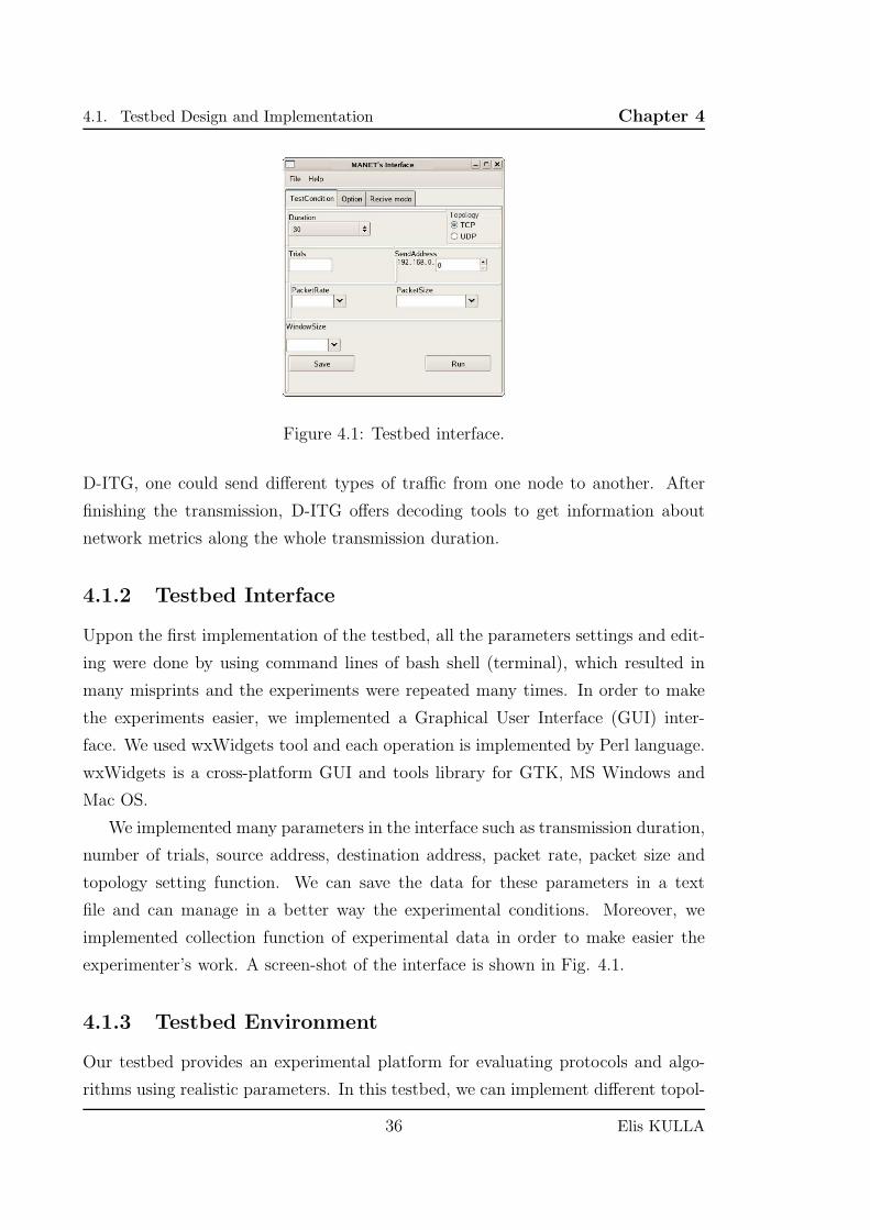
4.1. Testbed Design and Implementation Chapter 4
Figure 4.1: Testbed interface.
D-ITG, one could send different types of traffic from one node to another. After
finishing the transmission, D-ITG offers decoding tools to get information about
network metrics along the whole transmission duration.
4.1.2 Testbed Interface
Uppon the first implementation of the testbed, all the parameters settings and edit-
ing were done by using command lines of bash shell (terminal), which resulted in
many misprints and the experiments were repeated many times. In order to make
the experiments easier, we implemented a Graphical User Interface (GUI) inter-
face. We used wxWidgets tool and each operation is implemented by Perl language.
wxWidgets is a cross-platform GUI and tools library for GTK, MS Windows and
Mac OS.
We implemented many parameters in the interface such as transmission duration,
number of trials, source address, destination address, packet rate, packet size and
topology setting function. We can save the data for these parameters in a text
file and can manage in a better way the experimental conditions. Moreover, we
implemented collection function of experimental data in order to make easier the
experimenter’s work. A screen-shot of the interface is shown in Fig. 4.1.
4.1.3 Testbed Environment
Our testbed provides an experimental platform for evaluating protocols and algo-
rithms using realistic parameters. In this testbed, we can implement different topol-
36 Elis KULLA
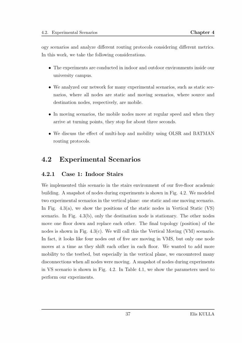
4.2. Experimental Scenarios Chapter 4
ogy scenarios and analyze different routing protocols considering different metrics.
In this work, we take the following considerations.
• The experiments are conducted in indoor and outdoor environments inside our
university campus.
• We analyzed our network for many experimental scenarios, such as static sce-
narios, where all nodes are static and moving scenarios, where source and
destination nodes, respectively, are mobile.
• In moving scenarios, the mobile nodes move at regular speed and when they
arrive at turning points, they stop for about three seconds.
• We discuss the effect of multi-hop and mobility using OLSR and BATMAN
routing protocols.
4.2 Experimental Scenarios
4.2.1 Case 1: Indoor Stairs
We implemented this scenario in the stairs environment of our five-floor academic
building. A snapshot of nodes during experiments is shown in Fig. 4.2. We modeled
two experimental scenarios in the vertical plane: one static and one moving scenario.
In Fig. 4.3(a), we show the positions of the static nodes in Vertical Static (VS)
scenario. In Fig. 4.3(b), only the destination node is stationary. The other nodes
move one floor down and replace each other. The final topology (position) of the
nodes is shown in Fig. 4.3(c). We will call this the Vertical Moving (VM) scenario.
In fact, it looks like four nodes out of five are moving in VMS, but only one node
moves at a time as they shift each other in each floor. We wanted to add more
mobility to the testbed, but especially in the vertical plane, we encountered many
disconnections when all nodes were moving. A snapshot of nodes during experiments
in VS scenario is shown in Fig. 4.2. In Table 4.1, we show the parameters used to
perform our experiments.
37 Elis KULLA
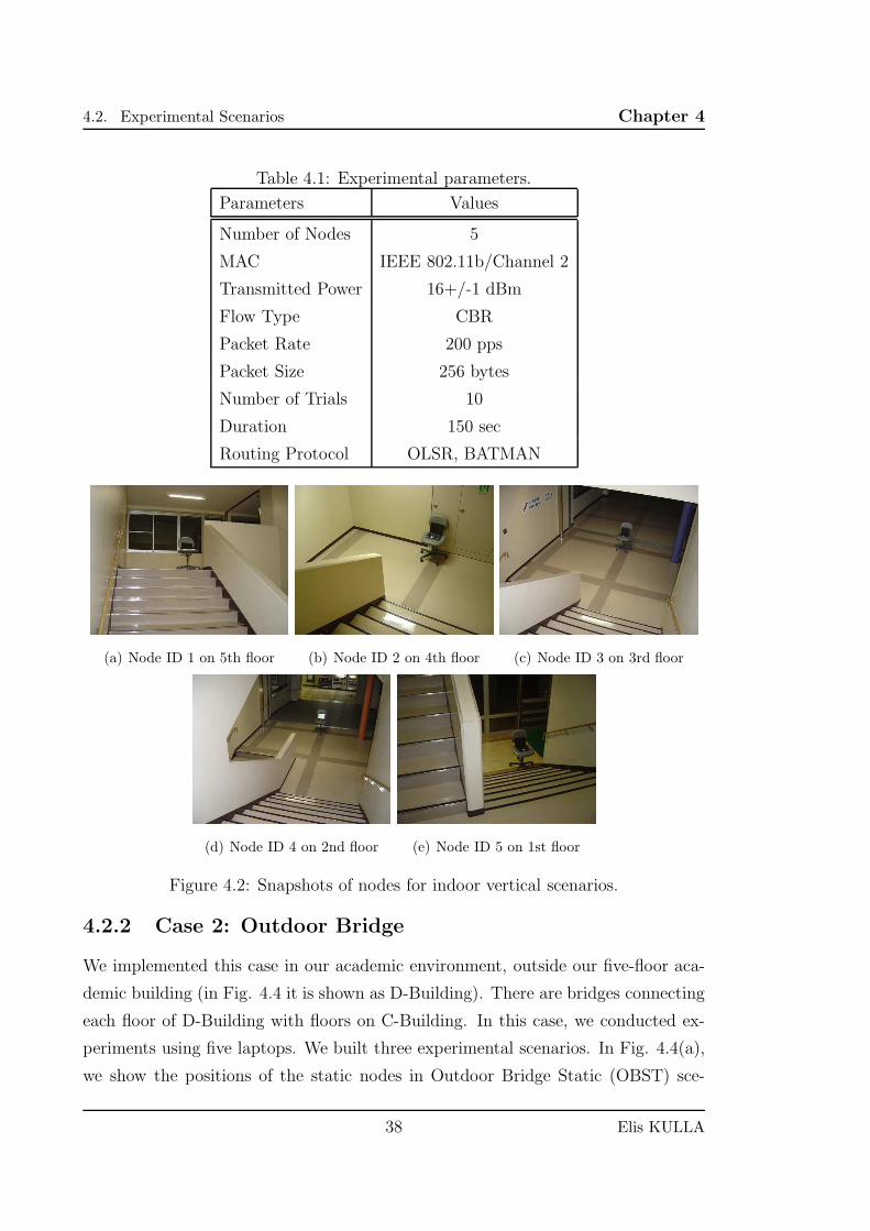
4.2. Experimental Scenarios Chapter 4
Table 4.1: Experimental parameters.
Parameters Values
Number of Nodes 5
MAC IEEE 802.11b/Channel 2
Transmitted Power 16+/-1 dBm
Flow Type CBR
Packet Rate 200 pps
Packet Size 256 bytes
Number of Trials 10
Duration 150 sec
Routing Protocol OLSR, BATMAN
(a) Node ID 1 on 5th floor (b) Node ID 2 on 4th floor (c) Node ID 3 on 3rd floor
(d) Node ID 4 on 2nd floor (e) Node ID 5 on 1st floor
Figure 4.2: Snapshots of nodes for indoor vertical scenarios.
4.2.2 Case 2: Outdoor Bridge
We implemented this case in our academic environment, outside our five-floor aca-
demic building (in Fig. 4.4 it is shown as D-Building). There are bridges connecting
each floor of D-Building with floors on C-Building. In this case, we conducted ex-
periments using five laptops. We built three experimental scenarios. In Fig. 4.4(a),
we show the positions of the static nodes in Outdoor Bridge Static (OBST) sce-
38 Elis KULLA
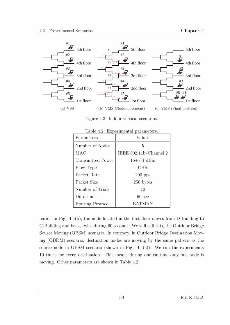
4.2. Experimental Scenarios Chapter 4
2nd floor
1st floor
3rd floor
4th floor
5th floor
#5
#4
#3
#2
#1
(a) VSS
2nd floor
1st floor
3rd floor
4th floor
5th floor
#5
#4
#3
#2
#1
#4
#3
#2
#1
(b) VMS (Node movement)
2nd floor
1st floor
3rd floor
4th floor
5th floor
#4#5
#3
#2
#1
(c) VMS (Final position)
Figure 4.3: Indoor vertical scenarios.
Table 4.2: Experimental parameters.
Parameters Values
Number of Nodes 5
MAC IEEE 802.11b/Channel 2
Transmitted Power 16+/-1 dBm
Flow Type CBR
Packet Rate 200 pps
Packet Size 256 bytes
Number of Trials 10
Duration 60 sec
Routing Protocol BATMAN
nario. In Fig. 4.4(b), the node located in the first floor moves from D-Building to
C-Building and back, twice during 60 seconds. We will call this, the Outdoor Bridge
Source Moving (OBSM) scenario. In contrary, in Outdoor Bridge Destination Mov-
ing (OBDM) scenario, destination nodes are moving by the same pattern as the
source node in OBSM scenario (shown in Fig. 4.4(c)). We run the experiments
10 times for every destination. This means during one runtime only one node is
moving. Other parameters are shown in Table 4.2
39 Elis KULLA
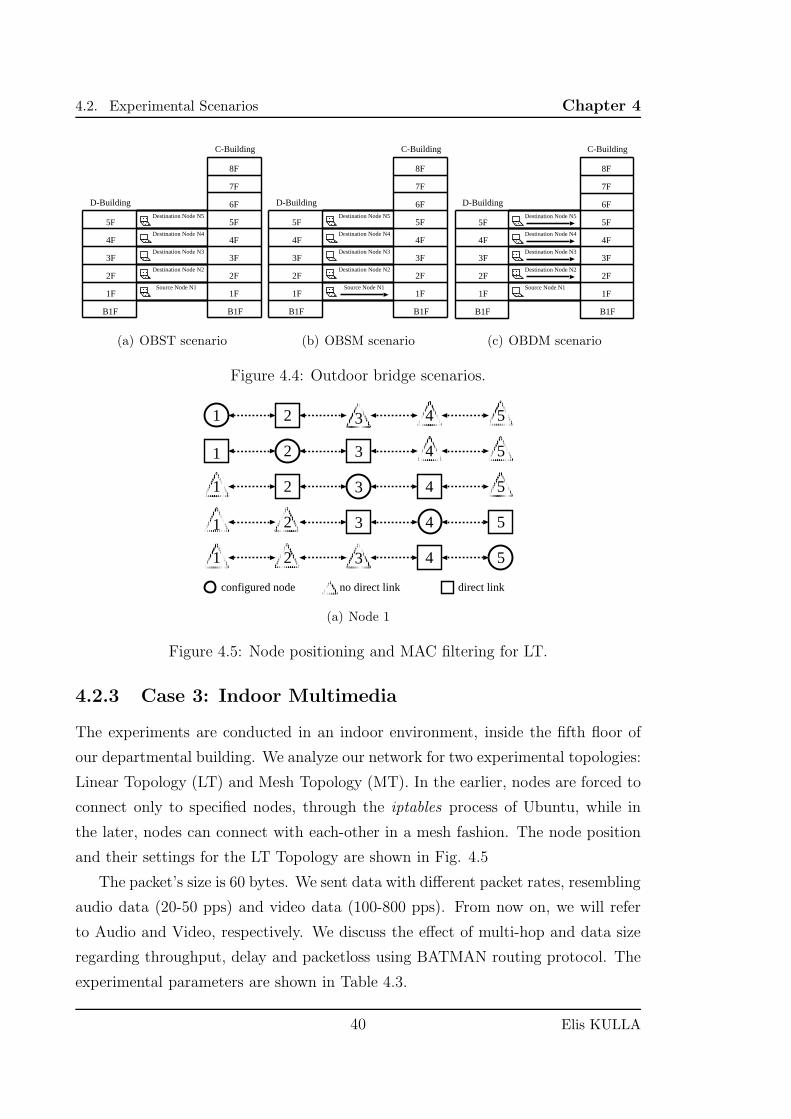
4.2. Experimental Scenarios Chapter 4
C-Building
D-Building
Source Node N1
Destination Node N2
Destination Node N3
Destination Node N4
Destination Node N55F
4F
3F
2F
1F
B1F B1F
1F
2F
3F
4F
5F
6F
7F
8F
(a) OBST scenario
D-Building
C-Building
Source Node N1
Destination Node N2
Destination Node N3
Destination Node N4
Destination Node N55F
4F
3F
2F
1F
B1F B1F
1F
2F
3F
4F
5F
6F
7F
8F
(b) OBSM scenario
D-Building
C-Building
Source Node N1
Destination Node N2
Destination Node N3
Destination Node N4
Destination Node N55F
4F
3F
2F
1F
B1F B1F
1F
2F
3F
4F
5F
6F
7F
8F
(c) OBDM scenario
Figure 4.4: Outdoor bridge scenarios.
2 41 53
configured node no direct link direct link
2 41 53
2 41 53
2 41 53
2 41 53
(a) Node 1
Figure 4.5: Node positioning and MAC filtering for LT.
4.2.3 Case 3: Indoor Multimedia
The experiments are conducted in an indoor environment, inside the fifth floor of
our departmental building. We analyze our network for two experimental topologies:
Linear Topology (LT) and Mesh Topology (MT). In the earlier, nodes are forced to
connect only to specified nodes, through the iptables process of Ubuntu, while in
the later, nodes can connect with each-other in a mesh fashion. The node position
and their settings for the LT Topology are shown in Fig. 4.5
The packet’s size is 60 bytes. We sent data with different packet rates, resembling
audio data (20-50 pps) and video data (100-800 pps). From now on, we will refer
to Audio and Video, respectively. We discuss the effect of multi-hop and data size
regarding throughput, delay and packetloss using BATMAN routing protocol. The
experimental parameters are shown in Table 4.3.
40 Elis KULLA
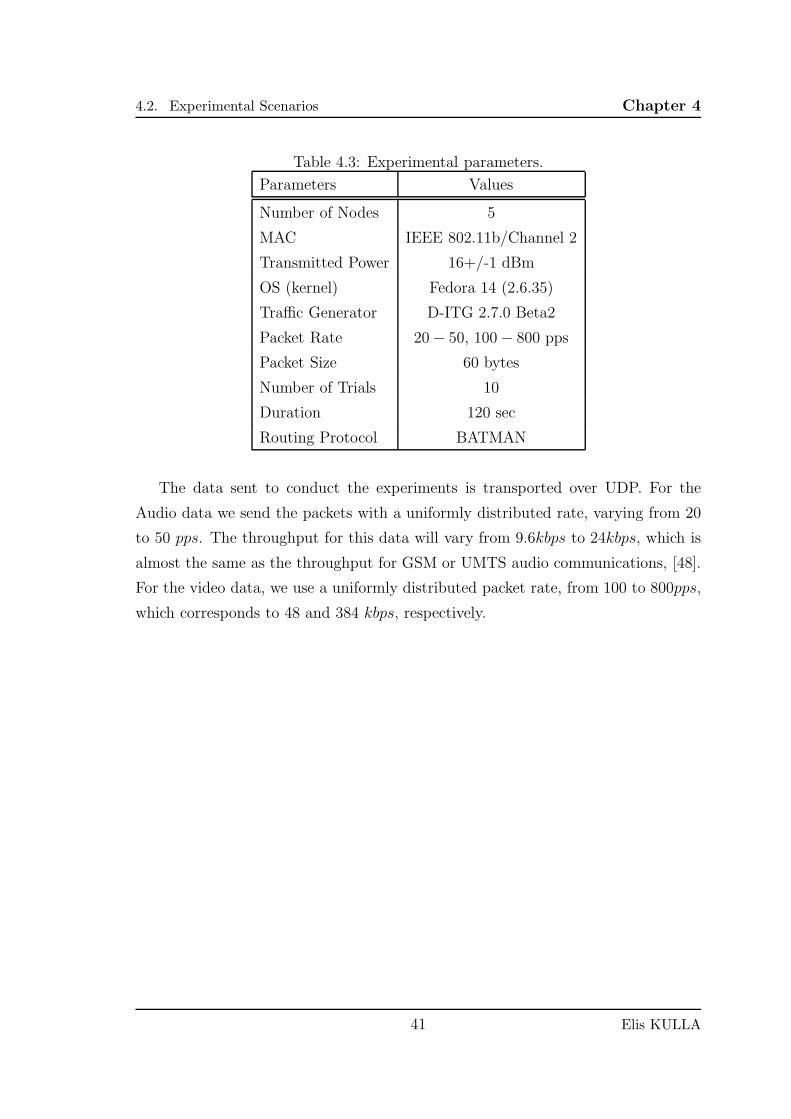
4.2. Experimental Scenarios Chapter 4
Table 4.3: Experimental parameters.
Parameters Values
Number of Nodes 5
MAC IEEE 802.11b/Channel 2
Transmitted Power 16+/-1 dBm
OS (kernel) Fedora 14 (2.6.35)
Traffic Generator D-ITG 2.7.0 Beta2
Packet Rate 20− 50, 100− 800 pps
Packet Size 60 bytes
Number of Trials 10
Duration 120 sec
Routing Protocol BATMAN
The data sent to conduct the experiments is transported over UDP. For the
Audio data we send the packets with a uniformly distributed rate, varying from 20
to 50 pps. The throughput for this data will vary from 9.6kbps to 24kbps, which is
almost the same as the throughput for GSM or UMTS audio communications, [48].
For the video data, we use a uniformly distributed packet rate, from 100 to 800pps,
which corresponds to 48 and 384 kbps, respectively.
41 Elis KULLA

Chapter 5
Simulators and Simulation
Scenarios
Simulation is the process of designing a model of a real system and conducting
experiments with this model for the purpose of understanding the behavior of the
system and/or evaluating various strategies for the operation of the system [49].
In MANET, simulations are very important to understand the behavior of rout-
ing protocols, addressing mechanisms, security algorithms, mobility models, and so
on. There are a number of network simulators such as NetSim [50], OPNET [51],
Network Simulator version 2/3 (NS2/NS3) [52, 53], which are usually used in the
network simulations. In our simulations, we use Network Simulator version 2 (NS2),
which is equipped with additional modules and analyzing tools.
5.1 NS2 Simulator System
5.1.1 Introduction
NS2 is a discrete event simulator. It is intended especially on Ad-hoc Networks. It is
a unix-based simulator build on different modules and uses TCL scripting language
for varying parameters and C++ structured code. Six modules are included in NS2:
nodes, links, SimpleLink objects, packets, agents, and applications. There are also
three helper modules: timers, random number generators, and error models. NS2
also consists of radio propagation models, traffic generators, topology generators for
different mobility models and so on.
43
5.2. Simulation Scenarios Chapter 5
5.1.2 Mobility Models
5.1.2.1 Random Waypoint Mobility (RWM) model
RWM model was first proposed by authors in [54] and it is used widely in simulating
MANETs. In NS2, this mobility model can be modeled by using the setdest tool. In
RWM model each node, uncorrelated to each-other, follows the following directions.
1. Selects a random starting position (W0) in the simulation area (L x W ).
2. Selects a random location in the area as the next waypoint (Wi).
3. Starts moving towards the destination Wi, with a randomly chosen speed
between Vmin and Vmax.
4. After reaching destination Wi, the node pauses for Tp seconds.
5. If Tmax is reached, end the movement.
6. Repeat steps 2-4.
The movement speed is a key parameter to decide the dynamism of the topology
and therefore changes in routes. For low speeds the topology is almost static and
for high speeds the topology becomes dynamic and the routes change frequently.
5.1.2.2 2D Random Walk Mobility Model (RW2)
In RW2, each instance moves with a speed and direction chosen at random with
the user-provided random variables until either a fixed distance has been walked
or until a fixed amount of time. If we hit one of the boundaries (specified by a
rectangle), of the model, we rebound on the boundary with a reflexive angle and
speed. Node movement is uncorrelated to each-other. This model is often identified
as a brownian motion model.
5.2 Simulation Scenarios
5.2.1 Case 1: Static2, OLSR and AODV
We prepared the simulation environment, taking care of the parameters during sim-
ulation time, as shown in Table 5.1. The size of the simulation area is 1000m x
44 Elis KULLA
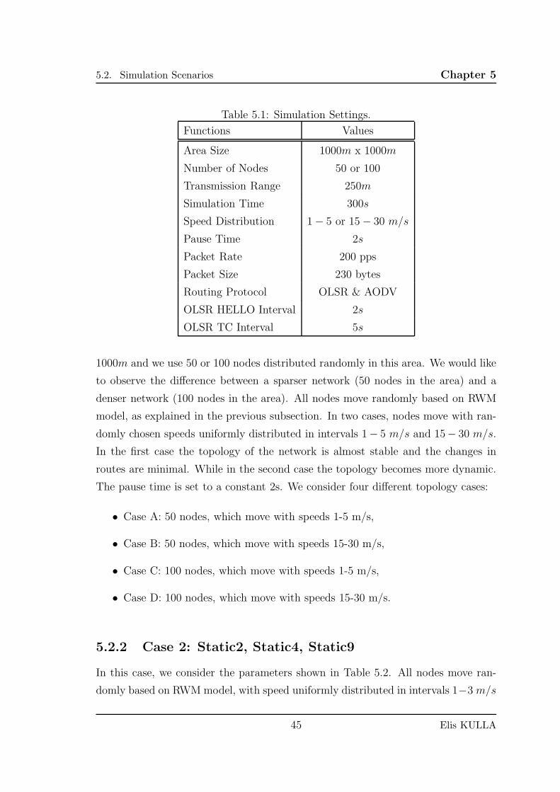
5.2. Simulation Scenarios Chapter 5
Table 5.1: Simulation Settings.
Functions Values
Area Size 1000m x 1000m
Number of Nodes 50 or 100
Transmission Range 250m
Simulation Time 300s
Speed Distribution 1− 5 or 15− 30 m/s
Pause Time 2s
Packet Rate 200 pps
Packet Size 230 bytes
Routing Protocol OLSR & AODV
OLSR HELLO Interval 2s
OLSR TC Interval 5s
1000m and we use 50 or 100 nodes distributed randomly in this area. We would like
to observe the difference between a sparser network (50 nodes in the area) and a
denser network (100 nodes in the area). All nodes move randomly based on RWM
model, as explained in the previous subsection. In two cases, nodes move with ran-
domly chosen speeds uniformly distributed in intervals 1− 5 m/s and 15− 30 m/s.
In the first case the topology of the network is almost stable and the changes in
routes are minimal. While in the second case the topology becomes more dynamic.
The pause time is set to a constant 2s. We consider four different topology cases:
• Case A: 50 nodes, which move with speeds 1-5 m/s,
• Case B: 50 nodes, which move with speeds 15-30 m/s,
• Case C: 100 nodes, which move with speeds 1-5 m/s,
• Case D: 100 nodes, which move with speeds 15-30 m/s.
5.2.2 Case 2: Static2, Static4, Static9
In this case, we consider the parameters shown in Table 5.2. All nodes move ran-
domly based on RWMmodel, with speed uniformly distributed in intervals 1−3 m/s
45 Elis KULLA
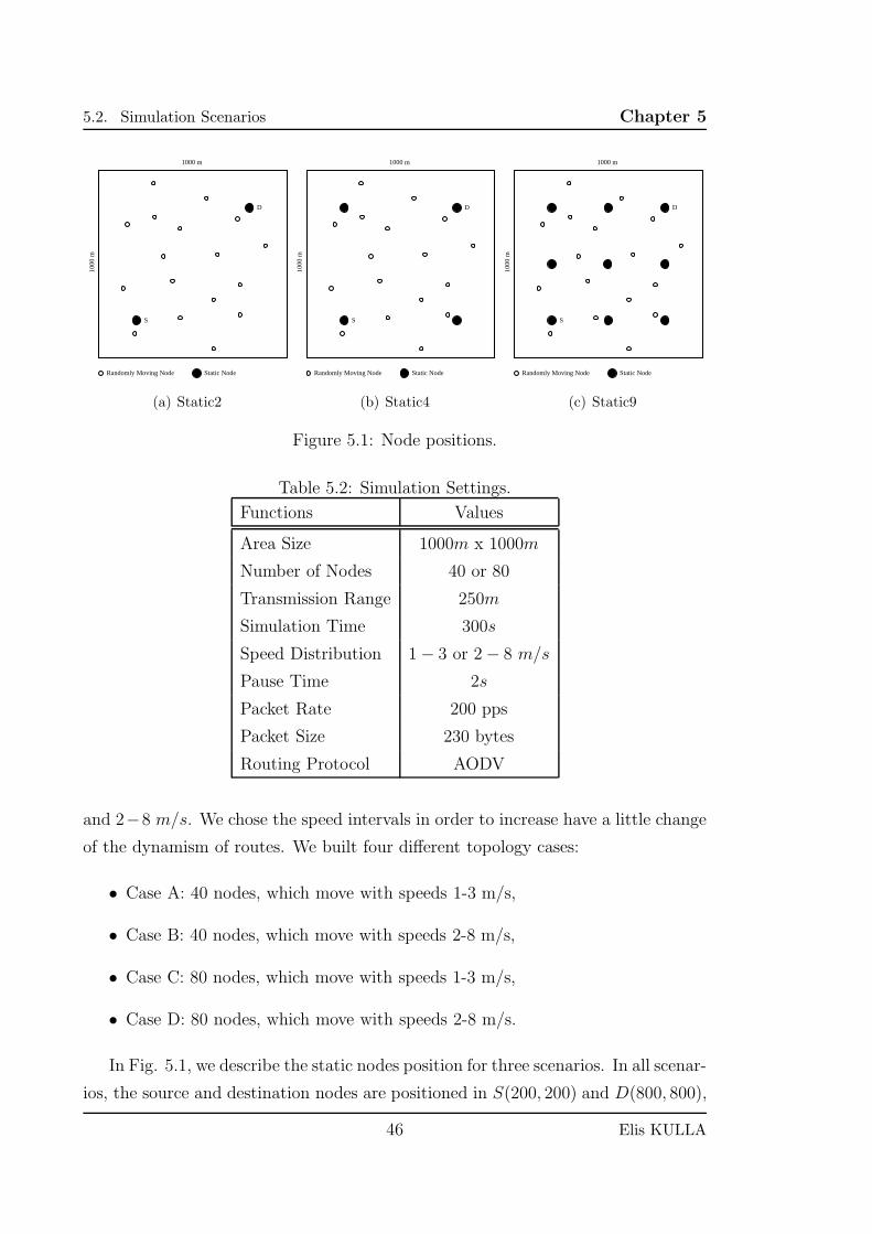
5.2. Simulation Scenarios Chapter 5
1000 m
1000
m
Randomly Moving Node Static Node
S
D
(a) Static2
1000 m
1000
m
Randomly Moving Node Static Node
S
D
(b) Static4
1000 m
1000
m
Randomly Moving Node Static Node
S
D
(c) Static9
Figure 5.1: Node positions.
Table 5.2: Simulation Settings.
Functions Values
Area Size 1000m x 1000m
Number of Nodes 40 or 80
Transmission Range 250m
Simulation Time 300s
Speed Distribution 1− 3 or 2− 8 m/s
Pause Time 2s
Packet Rate 200 pps
Packet Size 230 bytes
Routing Protocol AODV
and 2−8 m/s. We chose the speed intervals in order to increase have a little change
of the dynamism of routes. We built four different topology cases:
• Case A: 40 nodes, which move with speeds 1-3 m/s,
• Case B: 40 nodes, which move with speeds 2-8 m/s,
• Case C: 80 nodes, which move with speeds 1-3 m/s,
• Case D: 80 nodes, which move with speeds 2-8 m/s.
In Fig. 5.1, we describe the static nodes position for three scenarios. In all scenar-
ios, the source and destination nodes are positioned in S(200, 200) and D(800, 800),
46 Elis KULLA
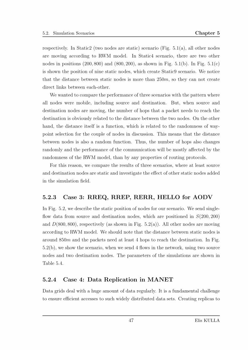
5.2. Simulation Scenarios Chapter 5
respectively. In Static2 (two nodes are static) scenario (Fig. 5.1(a), all other nodes
are moving according to RWM model. In Static4 scenario, there are two other
nodes in positions (200, 800) and (800, 200), as shown in Fig. 5.1(b). In Fig. 5.1(c)
is shown the position of nine static nodes, which create Static9 scenario. We notice
that the distance between static nodes is more than 250m, so they can not create
direct links between each-other.
We wanted to compare the performance of three scenarios with the pattern where
all nodes were mobile, including source and destination. But, when source and
destination nodes are moving, the number of hops that a packet needs to reach the
destination is obviously related to the distance between the two nodes. On the other
hand, the distance itself is a function, which is related to the randomness of way-
point selection for the couple of nodes in discussion. This means that the distance
between nodes is also a random function. Thus, the number of hops also changes
randomly and the performance of the communication will be mostly affected by the
randomness of the RWM model, than by any properties of routing protocols.
For this reason, we compare the results of three scenarios, where at least source
and destination nodes are static and investigate the effect of other static nodes added
in the simulation field.
5.2.3 Case 3: RREQ, RREP, RERR, HELLO for AODV
In Fig. 5.2, we describe the static position of nodes for our scenario. We send single-
flow data from source and destination nodes, which are positioned in S(200, 200)
and D(800, 800), respectively (as shown in Fig. 5.2(a)). All other nodes are moving
according to RWM model. We should note that the distance between static nodes is
around 850m and the packets need at least 4 hops to reach the destination. In Fig.
5.2(b), we show the scenario, when we send 4 flows in the network, using two source
nodes and two destination nodes. The parameters of the simulations are shown in
Table 5.4.
5.2.4 Case 4: Data Replication in MANET
Data grids deal with a huge amount of data regularly. It is a fundamental challenge
to ensure efficient accesses to such widely distributed data sets. Creating replicas to
47 Elis KULLA
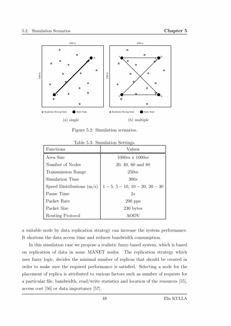
5.2. Simulation Scenarios Chapter 5
1000 m
1000
m
Randomly Moving Node Static Node
S
D
(a) single
1000 m
1000
m
Randomly Moving Node Static Node
S
S
D
D
(b) multiple
Figure 5.2: Simulation scenarios.
Table 5.3: Simulation Settings.
Functions Values
Area Size 1000m x 1000m
Number of Nodes 20, 40, 60 and 80
Transmission Range 250m
Simulation Time 300s
Speed Distributions (m/s) 1− 5, 5− 10, 10− 20, 20− 30
Pause Time 2s
Packet Rate 200 pps
Packet Size 230 bytes
Routing Protocol AODV
a suitable node by data replication strategy can increase the system performance.
It shortens the data access time and reduces bandwidth consumption.
In this simulation case we propose a realistic fuzzy-based system, which is based
on replication of data in some MANET nodes. The replication strategy which
uses fuzzy logic, decides the minimal number of replicas that should be created in
order to make sure the required performance is satisfied. Selecting a node for the
placement of replica is attributed to various factors such as number of requests for
a particular file, bandwidth, read/write statistics and location of the resources [55],
access cost [56] or data importance [57].
48 Elis KULLA
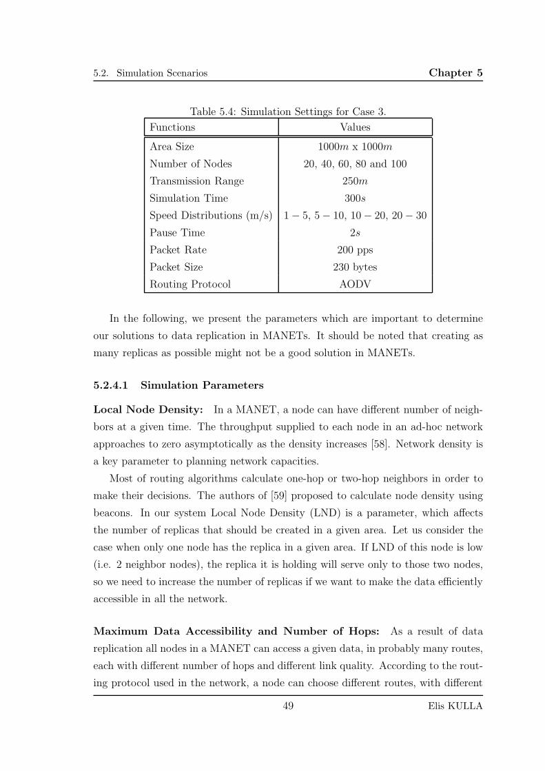
5.2. Simulation Scenarios Chapter 5
Table 5.4: Simulation Settings for Case 3.
Functions Values
Area Size 1000m x 1000m
Number of Nodes 20, 40, 60, 80 and 100
Transmission Range 250m
Simulation Time 300s
Speed Distributions (m/s) 1− 5, 5− 10, 10− 20, 20− 30
Pause Time 2s
Packet Rate 200 pps
Packet Size 230 bytes
Routing Protocol AODV
In the following, we present the parameters which are important to determine
our solutions to data replication in MANETs. It should be noted that creating as
many replicas as possible might not be a good solution in MANETs.
5.2.4.1 Simulation Parameters
Local Node Density: In a MANET, a node can have different number of neigh-
bors at a given time. The throughput supplied to each node in an ad-hoc network
approaches to zero asymptotically as the density increases [58]. Network density is
a key parameter to planning network capacities.
Most of routing algorithms calculate one-hop or two-hop neighbors in order to
make their decisions. The authors of [59] proposed to calculate node density using
beacons. In our system Local Node Density (LND) is a parameter, which affects
the number of replicas that should be created in a given area. Let us consider the
case when only one node has the replica in a given area. If LND of this node is low
(i.e. 2 neighbor nodes), the replica it is holding will serve only to those two nodes,
so we need to increase the number of replicas if we want to make the data efficiently
accessible in all the network.
Maximum Data Accessibility and Number of Hops: As a result of data
replication all nodes in a MANET can access a given data, in probably many routes,
each with different number of hops and different link quality. According to the rout-
ing protocol used in the network, a node can choose different routes, with different
49 Elis KULLA
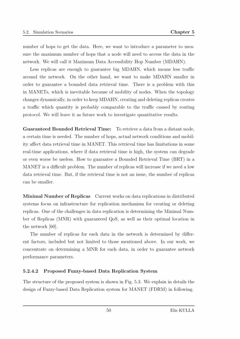
5.2. Simulation Scenarios Chapter 5
number of hops to get the data. Here, we want to introduce a parameter to mea-
sure the maximum number of hops that a node will need to access the data in the
network. We will call it Maximum Data Accessibility Hop Number (MDAHN).
Less replicas are enough to guarantee big MDAHN, which means less traffic
around the network. On the other hand, we want to make MDAHN smaller in
order to guarantee a bounded data retrieval time. There is a problem with this
in MANETs, which is inevitable because of mobility of nodes. When the topology
changes dynamically, in order to keep MDAHN, creating and deleting replicas creates
a traffic which quantity is probably comparable to the traffic caused by routing
protocol. We will leave it as future work to investigate quantitative results.
Guaranteed Bounded Retrieval Time: To retrieve a data from a distant node,
a certain time is needed. The number of hops, actual network conditions and mobil-
ity affect data retrieval time in MANET. This retrieval time has limitations in some
real-time applications, where if data retrieval time is high, the system can degrade
or even worse be useless. How to guarantee a Bounded Retrieval Time (BRT) in a
MANET is a difficult problem. The number of replicas will increase if we need a low
data retrieval time. But, if the retrieval time is not an issue, the number of replicas
can be smaller.
Minimal Number of Replicas Current works on data replications in distributed
systems focus on infrastructure for replication mechanism for creating or deleting
replicas. One of the challenges in data replication is determining the Minimal Num-
ber of Replicas (MNR) with guaranteed QoS, as well as their optimal location in
the network [60].
The number of replicas for each data in the network is determined by differ-
ent factors, included but not limited to those mentioned above. In our work, we
concentrate on determining a MNR for each data, in order to guarantee network
performance parameters.
5.2.4.2 Proposed Fuzzy-based Data Replication System
The structure of the proposed system is shown in Fig. 5.3. We explain in details the
design of Fuzzy-based Data Replication system for MANET (FDRM) in following.
50 Elis KULLA
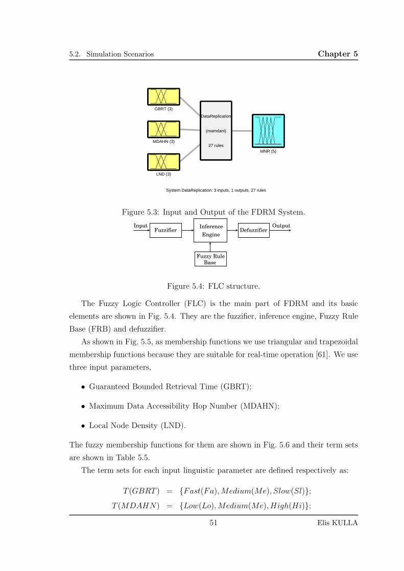
5.2. Simulation Scenarios Chapter 5
System DataReplication: 3 inputs, 1 outputs, 27 rules
GBRT (3)
MDAHN (3)
LND (3)
MNR (5)
DataReplication
(mamdani)
27 rules
Figure 5.3: Input and Output of the FDRM System.
FuzzifierInference
Engine
Fuzzy RuleBase
DefuzzifierOutputInput
Figure 5.4: FLC structure.
The Fuzzy Logic Controller (FLC) is the main part of FDRM and its basic
elements are shown in Fig. 5.4. They are the fuzzifier, inference engine, Fuzzy Rule
Base (FRB) and defuzzifier.
As shown in Fig. 5.5, as membership functions we use triangular and trapezoidal
membership functions because they are suitable for real-time operation [61]. We use
three input parameters,
• Guaranteed Bounded Retrieval Time (GBRT);
• Maximum Data Accessibility Hop Number (MDAHN);
• Local Node Density (LND).
The fuzzy membership functions for them are shown in Fig. 5.6 and their term sets
are shown in Table 5.5.
The term sets for each input linguistic parameter are defined respectively as:
T (GBRT ) = {Fast(Fa),Medium(Me), Slow(Sl)};T (MDAHN) = {Low(Lo),Medium(Me), High(Hi)};
51 Elis KULLA
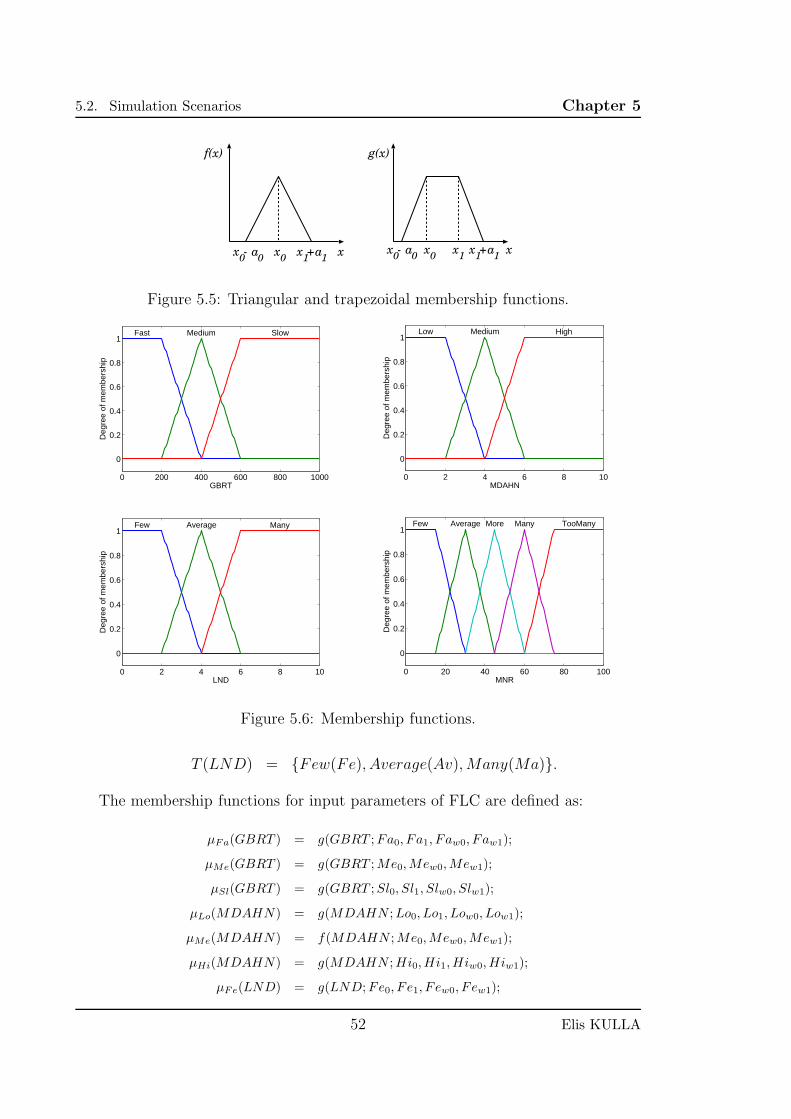
5.2. Simulation Scenarios Chapter 5
f(x) g(x)
x x xa0 0- x a
0 0-x a
1 1+
0xx a
1 1+x
0x1
Figure 5.5: Triangular and trapezoidal membership functions.
0 200 400 600 800 1000
0
0.2
0.4
0.6
0.8
1
GBRT
Deg
ree
of m
embe
rshi
p
Fast Medium Slow
0 2 4 6 8 10
0
0.2
0.4
0.6
0.8
1
MDAHN
Deg
ree
of m
embe
rshi
p
Low Medium High
0 2 4 6 8 10
0
0.2
0.4
0.6
0.8
1
LND
Deg
ree
of m
embe
rshi
p
Few Average Many
0 20 40 60 80 100
0
0.2
0.4
0.6
0.8
1
MNR
Deg
ree
of m
embe
rshi
p
Few Average TooManyMore Many
Figure 5.6: Membership functions.
T (LND) = {Few(Fe), Average(Av),Many(Ma)}.
The membership functions for input parameters of FLC are defined as:
µFa(GBRT ) = g(GBRT ;Fa0, Fa1, Faw0, Faw1);
µMe(GBRT ) = g(GBRT ;Me0,Mew0,Mew1);
µSl(GBRT ) = g(GBRT ;Sl0, Sl1, Slw0, Slw1);
µLo(MDAHN) = g(MDAHN ;Lo0, Lo1, Low0, Low1);
µMe(MDAHN) = f(MDAHN ;Me0,Mew0,Mew1);
µHi(MDAHN) = g(MDAHN ;Hi0, Hi1, Hiw0, Hiw1);
µFe(LND) = g(LND;Fe0, F e1, F ew0, F ew1);
52 Elis KULLA
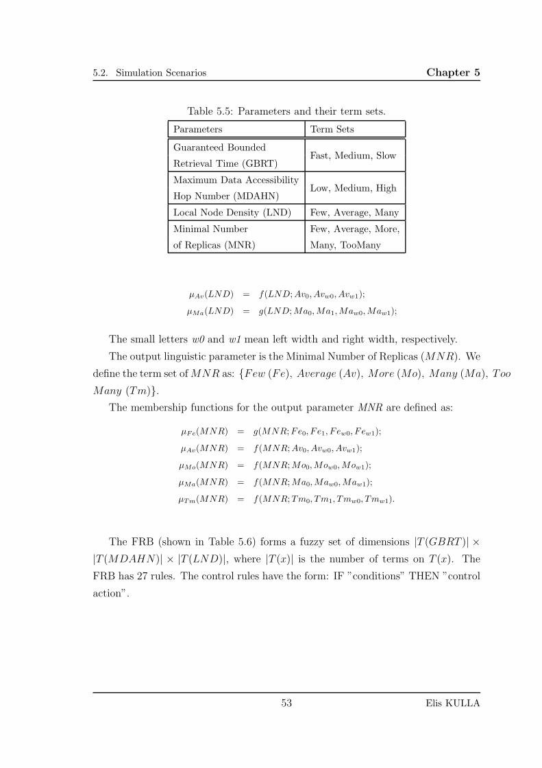
5.2. Simulation Scenarios Chapter 5
Table 5.5: Parameters and their term sets.
Parameters Term Sets
Guaranteed BoundedFast, Medium, Slow
Retrieval Time (GBRT)
Maximum Data AccessibilityLow, Medium, High
Hop Number (MDAHN)
Local Node Density (LND) Few, Average, Many
Minimal Number Few, Average, More,
of Replicas (MNR) Many, TooMany
µAv(LND) = f(LND;Av0, Avw0, Avw1);
µMa(LND) = g(LND;Ma0,Ma1,Maw0,Maw1);
The small letters w0 and w1 mean left width and right width, respectively.
The output linguistic parameter is the Minimal Number of Replicas (MNR). We
define the term set ofMNR as: {Few (Fe), Average (Av), More (Mo), Many (Ma), T oo
Many (Tm)}.The membership functions for the output parameter MNR are defined as:
µFe(MNR) = g(MNR;Fe0, F e1, F ew0, F ew1);
µAv(MNR) = f(MNR;Av0, Avw0, Avw1);
µMo(MNR) = f(MNR;Mo0,Mow0,Mow1);
µMa(MNR) = f(MNR;Ma0,Maw0,Maw1);
µTm(MNR) = f(MNR;Tm0, Tm1, Tmw0, Tmw1).
The FRB (shown in Table 5.6) forms a fuzzy set of dimensions |T (GBRT )| ×|T (MDAHN)| × |T (LND)|, where |T (x)| is the number of terms on T (x). The
FRB has 27 rules. The control rules have the form: IF ”conditions” THEN ”control
action”.
53 Elis KULLA
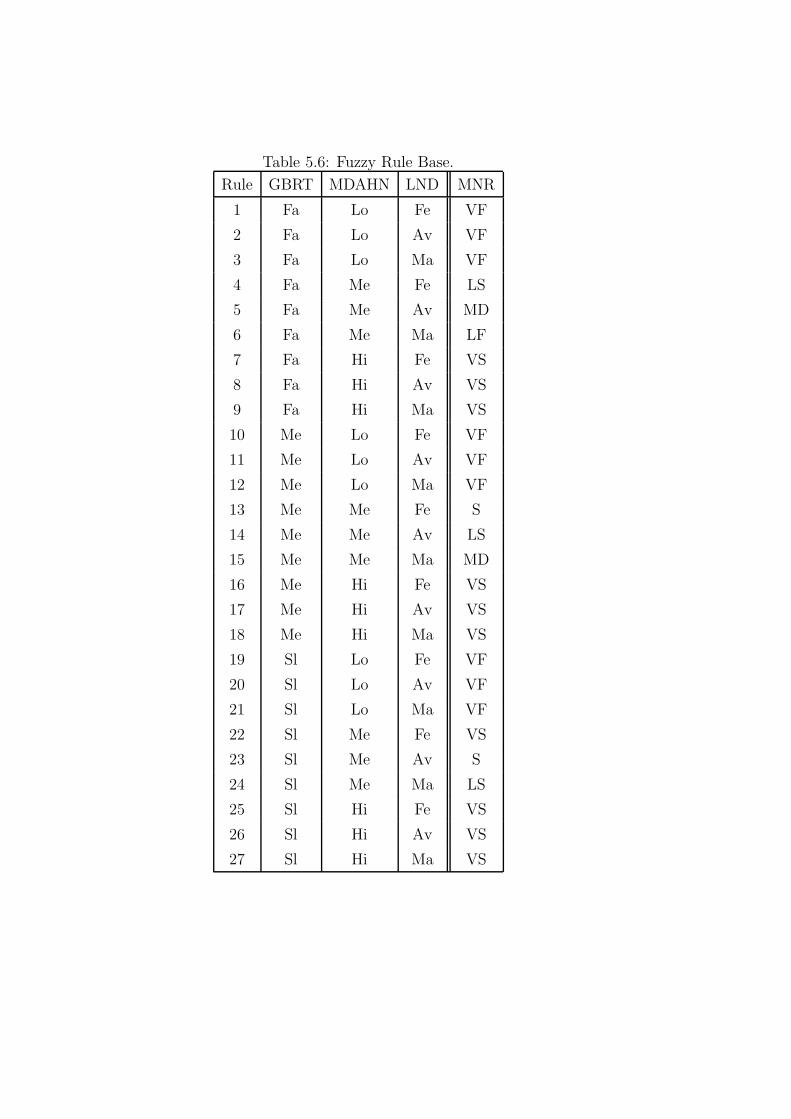
Table 5.6: Fuzzy Rule Base.
Rule GBRT MDAHN LND MNR
1 Fa Lo Fe VF
2 Fa Lo Av VF
3 Fa Lo Ma VF
4 Fa Me Fe LS
5 Fa Me Av MD
6 Fa Me Ma LF
7 Fa Hi Fe VS
8 Fa Hi Av VS
9 Fa Hi Ma VS
10 Me Lo Fe VF
11 Me Lo Av VF
12 Me Lo Ma VF
13 Me Me Fe S
14 Me Me Av LS
15 Me Me Ma MD
16 Me Hi Fe VS
17 Me Hi Av VS
18 Me Hi Ma VS
19 Sl Lo Fe VF
20 Sl Lo Av VF
21 Sl Lo Ma VF
22 Sl Me Fe VS
23 Sl Me Av S
24 Sl Me Ma LS
25 Sl Hi Fe VS
26 Sl Hi Av VS
27 Sl Hi Ma VS
Chapter 6
Experimental Results
IN this section we will present the result of our experiments. we implemented three
different cases in different environments and topologies. We show the results in
statistical display showing the median values of the entire communication. We also
show time-domain plots and average data in order to have a general understand-
ing of the performance. We used throughput, delay and packetloss as metrics for
performance assessment of OLSR, AODV and BATMAN routing protocols.
6.1 Case1: Indoor Stairs
We show the throughput results in Fig. 6.1 and Table 6.1. In Fig. 6.1(a) and Fig.
6.1(c), we show the throughput results for STAS scenario. For communication flow
from node 1 to node 2 and node 3, the throughput has only a few oscillations and
its average value is very close to DTR (409.6 kbps) for both protocols. When the
data flows from node 1 to node 4 or node 5 in STAS scenario the oscillations are
increased noticeably. The average throughput value for the communication from
node 1 to node 4 is almost 50 % lower than DTR and when data flows from node 1
to node 5 throughput is about 100 kbps (25% of DTR).
Also in SHIS scenario, for three-hop and four-hop communications we notice
oscillations. When we use BATMAN, the two-hop communication presents more
oscillations than in the case of OLSR. The average values for OLSR and BATMAN
decrease by 5% and 15% respectively, when the communications occurs in two hops.
For the average values of each flow see Table 6.1.
55
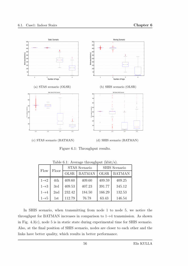
6.1. Case1: Indoor Stairs Chapter 6
0
50
100
150
200
250
300
350
400
450
500
1 2 3 4Number of hops
Bitra
te(k
bit/s
)
Static Scenario
(a) STAS scenario (OLSR)
0
50
100
150
200
250
300
350
400
450
500
1 2 3 4Number of hops
Bitra
te(k
bit/s
)
Moving Scenario
(b) SHIS scenario (OLSR)
1−2 1−3 1−4 1−50
100
200
300
400
500
600Static Stairs (STAS) Scenario
Th
rou
gh
pu
t (k
bit/s
)
(c) STAS scenario (BATMAN)
1−2 1−3 1−4 1−50
100
200
300
400
500
600
700
800Shift Stairs (SHIS) Scenario
TH
rou
gh
pu
t (k
bit/s
)
(d) SHIS scenario (BATMAN)
Figure 6.1: Throughput results.
Table 6.1: Average throughput (kbit/s).
Flow FloorSTAS Scenario SHIS Scenario
OLSR BATMAN OLSR BATMAN
1→2 4th 409.60 409.60 409.59 409.25
1→3 3rd 409.53 407.23 391.77 345.12
1→4 2nd 232.42 184.50 166.29 132.53
1→5 1st 112.79 76.78 63.43 146.54
In SHIS scenario, when transmitting from node 1 to node 5, we notice the
throughput for BATMAN increases in comparison to 1→4 transmission. As shown
in Fig. 4.3(c), node 5 is in static state during experimental time for SHIS scenario.
Also, at the final position of SHIS scenario, nodes are closer to each other and the
links have better quality, which results in better performance.
56 Elis KULLA
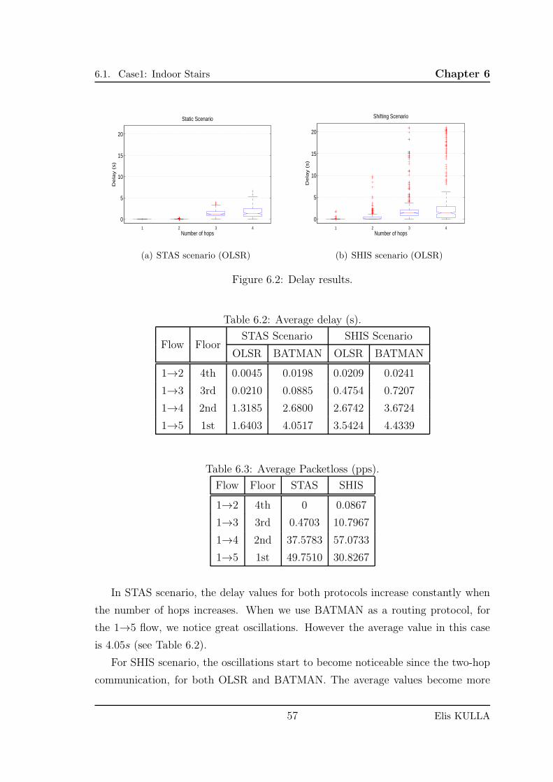
6.1. Case1: Indoor Stairs Chapter 6
0
5
10
15
20
1 2 3 4Number of hops
De
lay (
s)
Static Scenario
(a) STAS scenario (OLSR)
0
5
10
15
20
1 2 3 4Number of hops
Shifting Scenario
De
lay (
s)
(b) SHIS scenario (OLSR)
Figure 6.2: Delay results.
Table 6.2: Average delay (s).
Flow FloorSTAS Scenario SHIS Scenario
OLSR BATMAN OLSR BATMAN
1→2 4th 0.0045 0.0198 0.0209 0.0241
1→3 3rd 0.0210 0.0885 0.4754 0.7207
1→4 2nd 1.3185 2.6800 2.6742 3.6724
1→5 1st 1.6403 4.0517 3.5424 4.4339
Table 6.3: Average Packetloss (pps).
Flow Floor STAS SHIS
1→2 4th 0 0.0867
1→3 3rd 0.4703 10.7967
1→4 2nd 37.5783 57.0733
1→5 1st 49.7510 30.8267
In STAS scenario, the delay values for both protocols increase constantly when
the number of hops increases. When we use BATMAN as a routing protocol, for
the 1→5 flow, we notice great oscillations. However the average value in this case
is 4.05s (see Table 6.2).
For SHIS scenario, the oscillations start to become noticeable since the two-hop
communication, for both OLSR and BATMAN. The average values become more
57 Elis KULLA
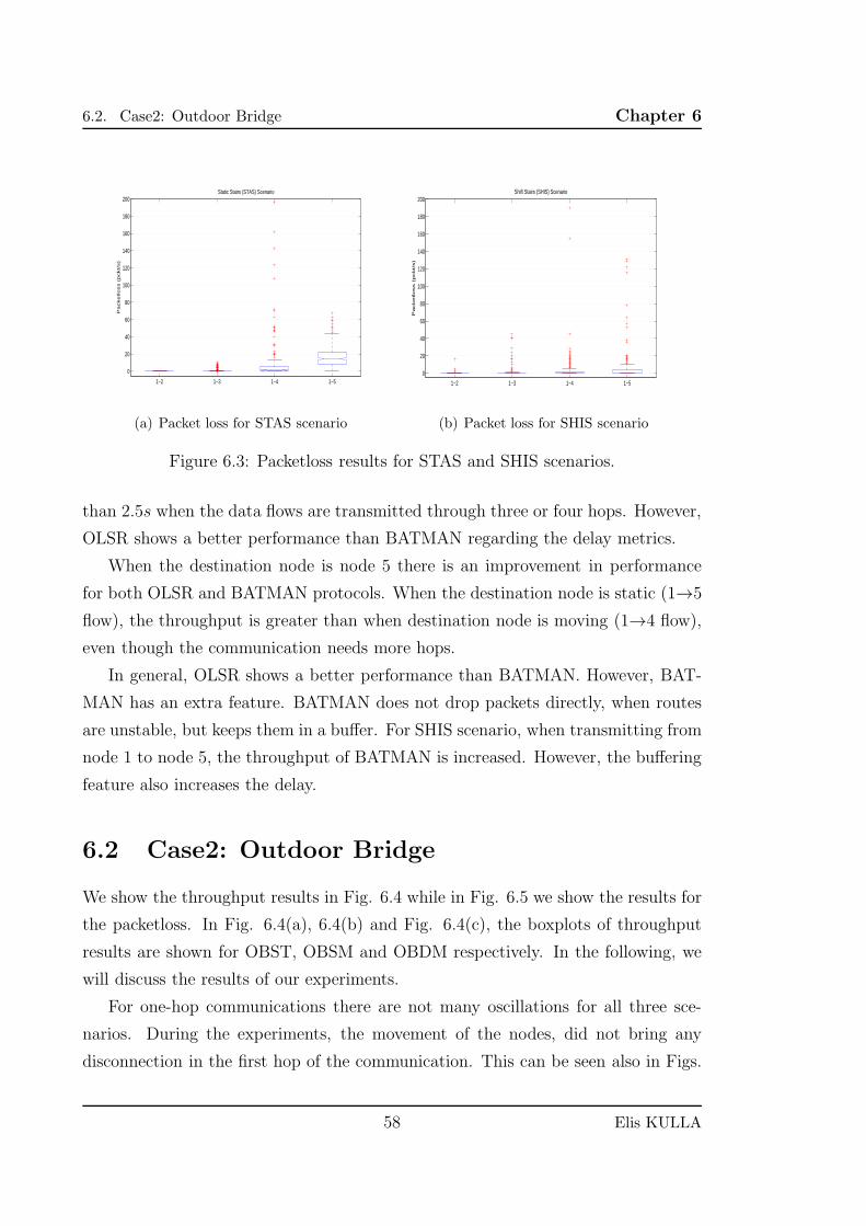
6.2. Case2: Outdoor Bridge Chapter 6
1−2 1−3 1−4 1−5
0
20
40
60
80
100
120
140
160
180
200Static Stairs (STAS) Scenario
Pa
cke
tlo
ss (
pckt/s)
(a) Packet loss for STAS scenario
1−2 1−3 1−4 1−5
0
20
40
60
80
100
120
140
160
180
200Shift Stairs (SHIS) Scenario
Pa
cke
tlo
ss (
pckt/s)
(b) Packet loss for SHIS scenario
Figure 6.3: Packetloss results for STAS and SHIS scenarios.
than 2.5s when the data flows are transmitted through three or four hops. However,
OLSR shows a better performance than BATMAN regarding the delay metrics.
When the destination node is node 5 there is an improvement in performance
for both OLSR and BATMAN protocols. When the destination node is static (1→5
flow), the throughput is greater than when destination node is moving (1→4 flow),
even though the communication needs more hops.
In general, OLSR shows a better performance than BATMAN. However, BAT-
MAN has an extra feature. BATMAN does not drop packets directly, when routes
are unstable, but keeps them in a buffer. For SHIS scenario, when transmitting from
node 1 to node 5, the throughput of BATMAN is increased. However, the buffering
feature also increases the delay.
6.2 Case2: Outdoor Bridge
We show the throughput results in Fig. 6.4 while in Fig. 6.5 we show the results for
the packetloss. In Fig. 6.4(a), 6.4(b) and Fig. 6.4(c), the boxplots of throughput
results are shown for OBST, OBSM and OBDM respectively. In the following, we
will discuss the results of our experiments.
For one-hop communications there are not many oscillations for all three sce-
narios. During the experiments, the movement of the nodes, did not bring any
disconnection in the first hop of the communication. This can be seen also in Figs.
58 Elis KULLA
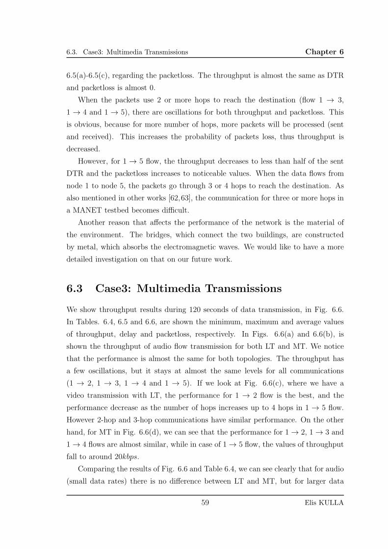
6.3. Case3: Multimedia Transmissions Chapter 6
6.5(a)-6.5(c), regarding the packetloss. The throughput is almost the same as DTR
and packetloss is almost 0.
When the packets use 2 or more hops to reach the destination (flow 1 → 3,
1 → 4 and 1 → 5), there are oscillations for both throughput and packetloss. This
is obvious, because for more number of hops, more packets will be processed (sent
and received). This increases the probability of packets loss, thus throughput is
decreased.
However, for 1 → 5 flow, the throughput decreases to less than half of the sent
DTR and the packetloss increases to noticeable values. When the data flows from
node 1 to node 5, the packets go through 3 or 4 hops to reach the destination. As
also mentioned in other works [62,63], the communication for three or more hops in
a MANET testbed becomes difficult.
Another reason that affects the performance of the network is the material of
the environment. The bridges, which connect the two buildings, are constructed
by metal, which absorbs the electromagnetic waves. We would like to have a more
detailed investigation on that on our future work.
6.3 Case3: Multimedia Transmissions
We show throughput results during 120 seconds of data transmission, in Fig. 6.6.
In Tables. 6.4, 6.5 and 6.6, are shown the minimum, maximum and average values
of throughput, delay and packetloss, respectively. In Figs. 6.6(a) and 6.6(b), is
shown the throughput of audio flow transmission for both LT and MT. We notice
that the performance is almost the same for both topologies. The throughput has
a few oscillations, but it stays at almost the same levels for all communications
(1 → 2, 1 → 3, 1 → 4 and 1 → 5). If we look at Fig. 6.6(c), where we have a
video transmission with LT, the performance for 1 → 2 flow is the best, and the
performance decrease as the number of hops increases up to 4 hops in 1 → 5 flow.
However 2-hop and 3-hop communications have similar performance. On the other
hand, for MT in Fig. 6.6(d), we can see that the performance for 1 → 2, 1 → 3 and
1 → 4 flows are almost similar, while in case of 1 → 5 flow, the values of throughput
fall to around 20kbps.
Comparing the results of Fig. 6.6 and Table 6.4, we can see clearly that for audio
(small data rates) there is no difference between LT and MT, but for larger data
59 Elis KULLA
6.3. Case3: Multimedia Transmissions Chapter 6
1−>2 1−>3 1−>4 1−>50
100
200
300
400
500
600
700
800BATMAN OBST
Bitr
ate
(kbp
s)
(a) bitrate (OBST)
1−>2 1−>3 1−>4 1−>50
100
200
300
400
500
600
700
800BATMAN OBSM
BItr
ate
(kbp
s)
(b) bitrate (OBSM)
BIt
rate
(kb
ps)
BATMAN OBDM
1−>2 1−>3 1−>4 1−>50
100
200
300
400
500
600
700
800
(c) bitrate (OBDM)
Figure 6.4: Bitrate experimental results.
rates, in MT case the average throughput decreases and the oscillations increase. In
LT scheme, one node can receive OGMs only from its neighbors, so the number of
received OGMs from other nodes is zero. This means that the route from node 1 to
other nodes, are always known and unchangeable. However there is an unchangeable
4-hop transmission from node 1 to node 5. In the MT scheme, lets say, node 1 wants
to transmit to node 5 with the high rate video transmission of 48-384 pps. First, the
best 1-hop neighbor is node 2 and it starts to send packets to node 2. Meanwhile,
the 1 → 2 link is busy and node 1 receives from node 3 some OGMs broadcast by
node 5, so that node 3 becomes the best 1-hop neighbor. Then, while the 1 → 3
link is busy, it will happen the opposite. This instability in routes brings oscillations
and decrease in throughput. The packetloss, shown in Table 6.6, is closely related
to throughput and it has a similar behavior. We can see that for audio data the
packetloss is very small so the performance is very good.
60 Elis KULLA
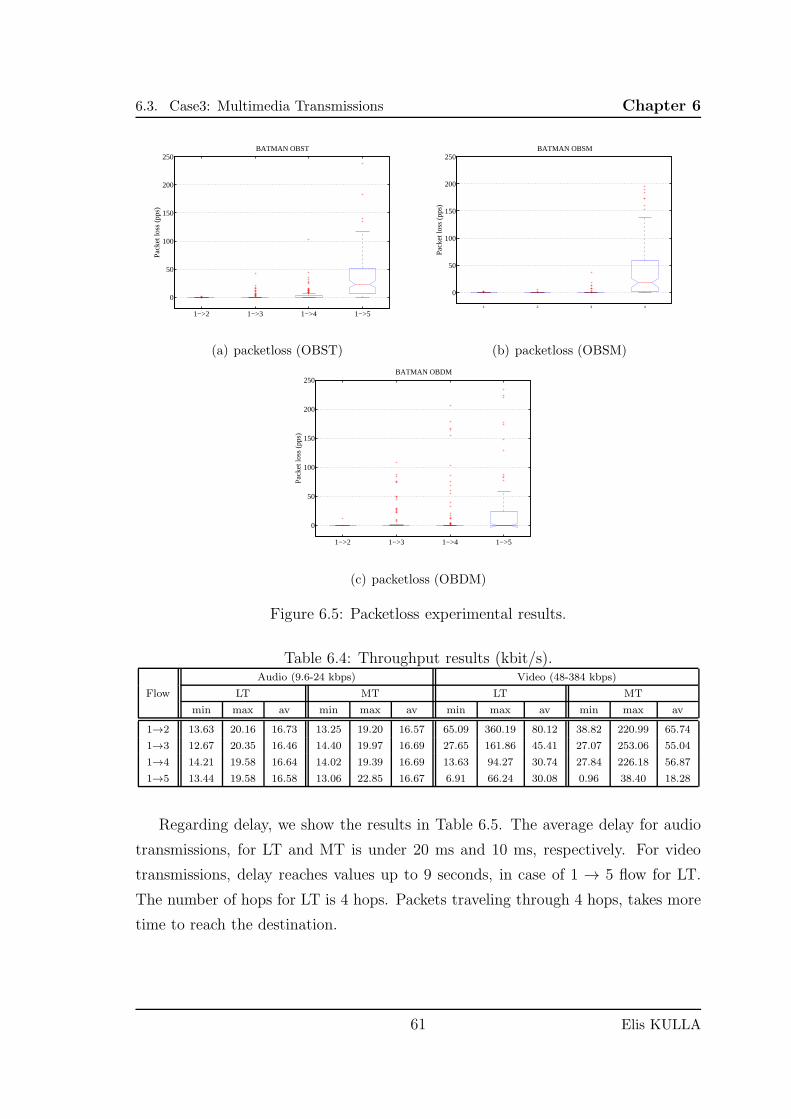
6.3. Case3: Multimedia Transmissions Chapter 6
1−>2 1−>3 1−>4 1−>5
0
50
100
150
200
250BATMAN OBST
Pac
ket l
oss
(pps
)
(a) packetloss (OBST)
0
50
100
150
200
250
1 2 3 4
BATMAN OBSM
Pack
et lo
ss (
pps)
(b) packetloss (OBSM)
1−>2 1−>3 1−>4 1−>5
0
50
100
150
200
250BATMAN OBDM
Pac
ket l
oss
(pps
)
(c) packetloss (OBDM)
Figure 6.5: Packetloss experimental results.
Table 6.4: Throughput results (kbit/s).
Flow
Audio (9.6-24 kbps) Video (48-384 kbps)
LT MT LT MT
min max av min max av min max av min max av
1→2 13.63 20.16 16.73 13.25 19.20 16.57 65.09 360.19 80.12 38.82 220.99 65.74
1→3 12.67 20.35 16.46 14.40 19.97 16.69 27.65 161.86 45.41 27.07 253.06 55.04
1→4 14.21 19.58 16.64 14.02 19.39 16.69 13.63 94.27 30.74 27.84 226.18 56.87
1→5 13.44 19.58 16.58 13.06 22.85 16.67 6.91 66.24 30.08 0.96 38.40 18.28
Regarding delay, we show the results in Table 6.5. The average delay for audio
transmissions, for LT and MT is under 20 ms and 10 ms, respectively. For video
transmissions, delay reaches values up to 9 seconds, in case of 1 → 5 flow for LT.
The number of hops for LT is 4 hops. Packets traveling through 4 hops, takes more
time to reach the destination.
61 Elis KULLA
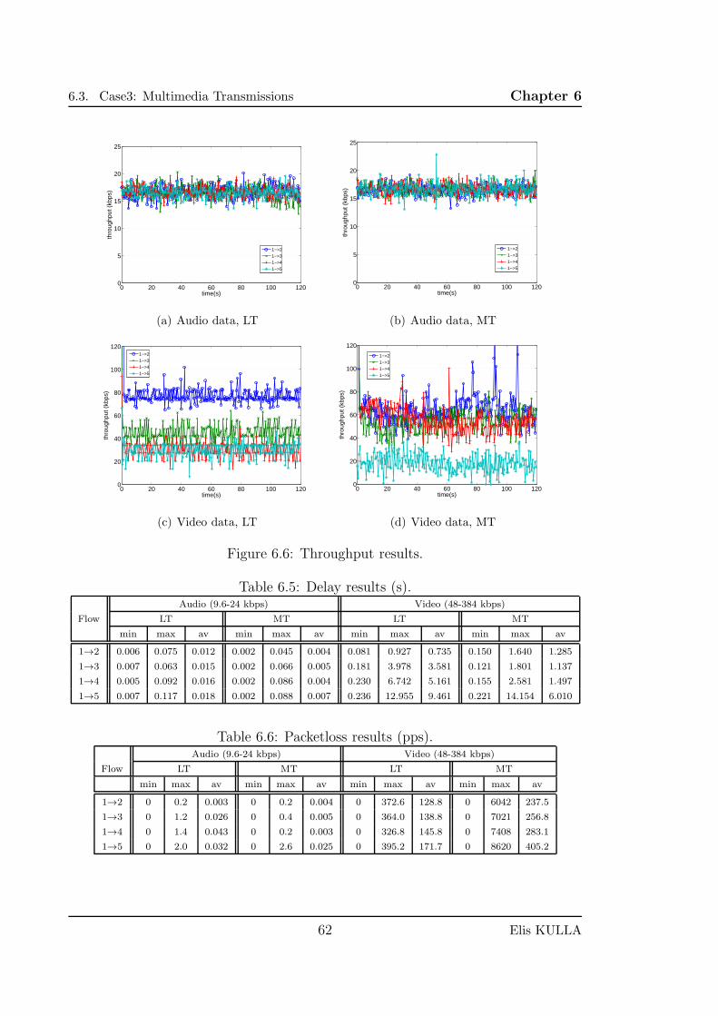
6.3. Case3: Multimedia Transmissions Chapter 6
0 20 40 60 80 100 1200
5
10
15
20
25
time(s)
thro
ughp
ut (
kbps
)
1−>21−>31−>41−>5
(a) Audio data, LT
0 20 40 60 80 100 1200
5
10
15
20
25
time(s)
thro
ughp
ut (
kbps
)
1−>21−>31−>41−>5
(b) Audio data, MT
0 20 40 60 80 100 1200
20
40
60
80
100
120
time(s)
thro
ughp
ut (
kbps
)
1−>21−>31−>41−>5
(c) Video data, LT
0 20 40 60 80 100 1200
20
40
60
80
100
120
time(s)
thro
ughp
ut (
kbps
)
1−>21−>31−>41−>5
(d) Video data, MT
Figure 6.6: Throughput results.
Table 6.5: Delay results (s).
Flow
Audio (9.6-24 kbps) Video (48-384 kbps)
LT MT LT MT
min max av min max av min max av min max av
1→2 0.006 0.075 0.012 0.002 0.045 0.004 0.081 0.927 0.735 0.150 1.640 1.285
1→3 0.007 0.063 0.015 0.002 0.066 0.005 0.181 3.978 3.581 0.121 1.801 1.137
1→4 0.005 0.092 0.016 0.002 0.086 0.004 0.230 6.742 5.161 0.155 2.581 1.497
1→5 0.007 0.117 0.018 0.002 0.088 0.007 0.236 12.955 9.461 0.221 14.154 6.010
Table 6.6: Packetloss results (pps).
Flow
Audio (9.6-24 kbps) Video (48-384 kbps)
LT MT LT MT
min max av min max av min max av min max av
1→2 0 0.2 0.003 0 0.2 0.004 0 372.6 128.8 0 6042 237.5
1→3 0 1.2 0.026 0 0.4 0.005 0 364.0 138.8 0 7021 256.8
1→4 0 1.4 0.043 0 0.2 0.003 0 326.8 145.8 0 7408 283.1
1→5 0 2.0 0.032 0 2.6 0.025 0 395.2 171.7 0 8620 405.2
62 Elis KULLA
Chapter 7
Simulation Results
We conducted simulations for different scenarios in our NS2-based simulation sys-
tem We consider four simulation cases for different applications of MANETs. We
investigate the effect of static components in the performance of MANET routing
protocols. A data replication simulation framework is also evaluated in the fourth
case.
7.1 Case 1: Static Source and Destination for
OLSR and AODV
In Fig. 7.1, we show the distance between source and destination nodes. It is also
shown the number of hops that packets need to go from source to destination. All
nodes are moving according to RWM model. We will refer to this as All Move
(ALMOV) scenario. We can see that the number of hops is directly related to the
distance between nodes.
The average values of throughput are shown in Table 7.1 and Table 7.2. In AL-
MOV scenario, the distance changes randomly in different topologies. The number
of hops also changes with the change of distance. In SDSTA scenario the distance
is fixed to 848.53 meters as shown in Table 7.1.
We conducted simulations for 4 topologies considering OLSR and AODV proto-
col. The OLSR patch can be found in [64]. For all cases, we show distance versus
number of hops for ALMOV and SDSTA scenarios, in Fig. 7.1 and Fig. 7.2, respec-
tively. The data sent from source node to destination node is CBR type transported
63
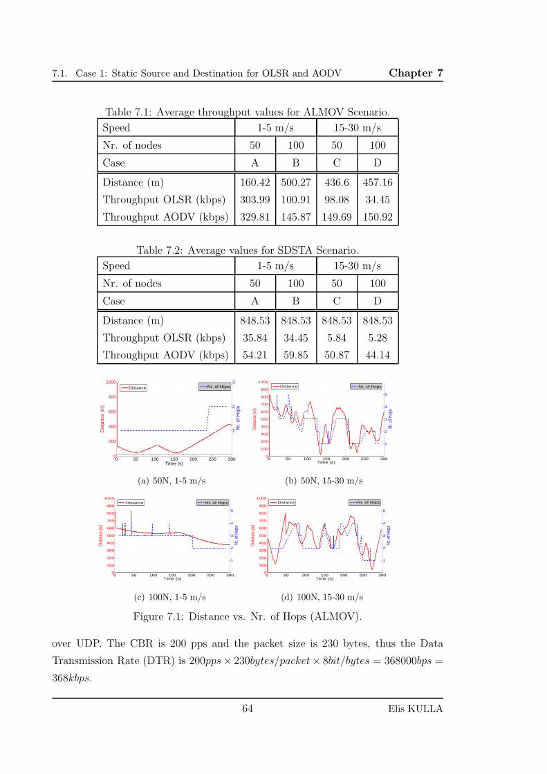
7.1. Case 1: Static Source and Destination for OLSR and AODV Chapter 7
Table 7.1: Average throughput values for ALMOV Scenario.
Speed 1-5 m/s 15-30 m/s
Nr. of nodes 50 100 50 100
Case A B C D
Distance (m) 160.42 500.27 436.6 457.16
Throughput OLSR (kbps) 303.99 100.91 98.08 34.45
Throughput AODV (kbps) 329.81 145.87 149.69 150.92
Table 7.2: Average values for SDSTA Scenario.
Speed 1-5 m/s 15-30 m/s
Nr. of nodes 50 100 50 100
Case A B C D
Distance (m) 848.53 848.53 848.53 848.53
Throughput OLSR (kbps) 35.84 34.45 5.84 5.28
Throughput AODV (kbps) 54.21 59.85 50.87 44.14
0 50 100 150 200 250 3000
200
400
600
800
1000
Dis
tanc
e (m
)
Time (s)
1
2
3
Nr.
of H
ops
Distance Nr. of Hops
(a) 50N, 1-5 m/s
0 50 100 150 200 250 3000
100
200
300
400
500
600
700
800
900
1000
Dist
ance
(m)
Time (s)
1
2
3
4
5Nr
. of H
ops
Distance Nr. of Hops
(b) 50N, 15-30 m/s
0 50 100 150 200 250 3000
100
200
300
400
500
600
700
800
900
1000
Dist
ance
(m)
Time (s)
1
2
3
4
5
Nr. o
f Hop
s
Distance Nr. of Hops
(c) 100N, 1-5 m/s
0 50 100 150 200 250 3000
100
200
300
400
500
600
700
800
900
1000
Dist
ance
(m)
Time (s)
1
2
3
4
5
Nr. o
f Hop
s
Distance Nr. of Hops
(d) 100N, 15-30 m/s
Figure 7.1: Distance vs. Nr. of Hops (ALMOV).
over UDP. The CBR is 200 pps and the packet size is 230 bytes, thus the Data
Transmission Rate (DTR) is 200pps× 230bytes/packet× 8bit/bytes = 368000bps =
368kbps.
64 Elis KULLA
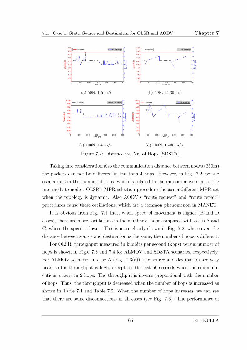
7.1. Case 1: Static Source and Destination for OLSR and AODV Chapter 7
0 50 100 150 200 250 3000
100
200
300
400
500
600
700
800
900
1000
Dist
ance
(m)
Time (s)
1
2
3
4
5
6
7
8
Nr. o
f Hop
s
Distance Nr. of Hops
(a) 50N, 1-5 m/s
0 50 100 150 200 250 3000
100
200
300
400
500
600
700
800
900
1000
Dist
ance
(m)
Time (s)
1
2
3
4
5
6
7
8
Nr. o
f Hop
s
Distance Nr. of Hops
(b) 50N, 15-30 m/s
0 50 100 150 200 250 3000
100
200
300
400
500
600
700
800
900
1000
Dist
ance
(m)
Time (s)
1
2
3
4
5
6
7
8
Nr. o
f Hop
s
Distance Nr. of Hops
(c) 100N, 1-5 m/s
0 50 100 150 200 250 3000
100
200
300
400
500
600
700
800
900
1000
Dist
ance
(m)
Time (s)
1
2
3
4
5
6
7
8
Nr. o
f Hop
s
Distance Nr. of Hops
(d) 100N, 15-30 m/s
Figure 7.2: Distance vs. Nr. of Hops (SDSTA).
Taking into consideration also the communication distance between nodes (250m),
the packets can not be delivered in less than 4 hops. However, in Fig. 7.2, we see
oscillations in the number of hops, which is related to the random movement of the
intermediate nodes. OLSR’s MPR selection procedure chooses a different MPR set
when the topology is dynamic. Also AODV’s “route request” and “route repair”
procedures cause these oscillations, which are a common phenomenon in MANET.
It is obvious from Fig. 7.1 that, when speed of movement is higher (B and D
cases), there are more oscillations in the number of hops compared with cases A and
C, where the speed is lower. This is more clearly shown in Fig. 7.2, where even the
distance between source and destination is the same, the number of hops is different.
For OLSR, throughput measured in kilobits per second (kbps) versus number of
hops is shown in Figs. 7.3 and 7.4 for ALMOV and SDSTA scenarios, respectively.
For ALMOV scenario, in case A (Fig. 7.3(a)), the source and destination are very
near, so the throughput is high, except for the last 50 seconds when the communi-
cations occurs in 2 hops. The throughput is inverse proportional with the number
of hops. Thus, the throughput is decreased when the number of hops is increased as
shown in Table 7.1 and Table 7.2. When the number of hops increases, we can see
that there are some disconnections in all cases (see Fig. 7.3). The performance of
65 Elis KULLA
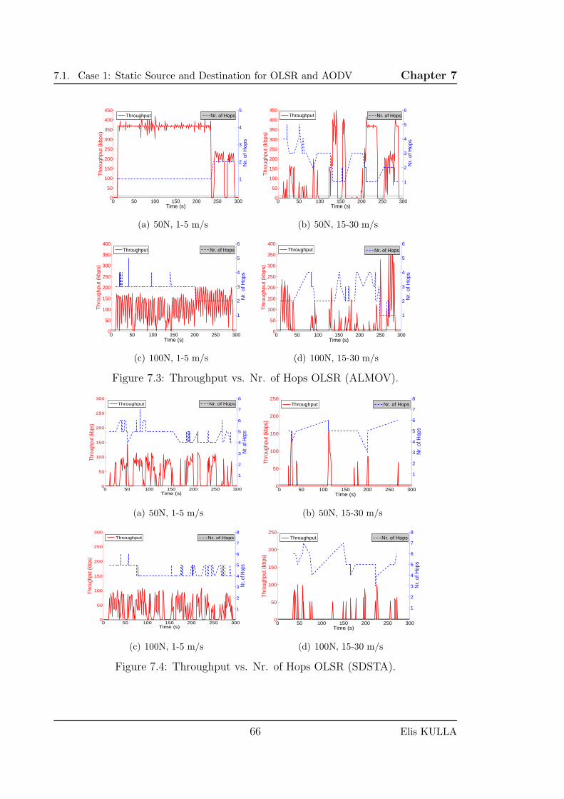
7.1. Case 1: Static Source and Destination for OLSR and AODV Chapter 7
0 50 100 150 200 250 3000
50
100
150
200
250
300
350
400
450
Thr
ough
put (
kbps
)
Time (s)
1
2
3
4
5
Nr.
of H
ops
Throughput Nr. of Hops
(a) 50N, 1-5 m/s
0 50 100 150 200 250 3000
50
100
150
200
250
300
350
400
450
Thr
ough
put (
kbps
)
Time (s)
1
2
3
4
5
6
Nr.
of H
ops
Throughput Nr. of Hops
(b) 50N, 15-30 m/s
0 50 100 150 200 250 3000
50
100
150
200
250
300
350
400
Thr
ough
put (
kbps
)
Time (s)
1
2
3
4
5
6N
r. o
f Hop
s
Throughput Nr. of Hops
(c) 100N, 1-5 m/s
0 50 100 150 200 250 3000
50
100
150
200
250
300
350
400
Thr
ough
put (
kbps
)
Time (s)
1
2
3
4
5
6
Nr.
of H
ops
Throughput Nr. of Hops
(d) 100N, 15-30 m/s
Figure 7.3: Throughput vs. Nr. of Hops OLSR (ALMOV).
0 50 100 150 200 250 3000
50
100
150
200
250
300
Thro
ughp
ut (k
bps)
Time (s)
1
2
3
4
5
6
7
8
Nr. o
f Hop
s
Throughput Nr. of Hops
(a) 50N, 1-5 m/s
0 50 100 150 200 250 3000
50
100
150
200
250
Thro
ughp
ut (k
bps)
Time (s)
1
2
3
4
5
6
7
8
Nr.
of H
ops
Throughput Nr. of Hops
(b) 50N, 15-30 m/s
0 50 100 150 200 250 3000
50
100
150
200
250
300
Thro
ughp
ut (k
bps)
Time (s)
1
2
3
4
5
6
7
8
Nr. o
f Hop
s
Throughput Nr. of Hops
(c) 100N, 1-5 m/s
0 50 100 150 200 250 3000
50
100
150
200
250
Thro
ughp
ut (k
bps)
Time (s)
1
2
3
4
5
6
7
8
Nr.
of H
ops
Throughput Nr. of Hops
(d) 100N, 15-30 m/s
Figure 7.4: Throughput vs. Nr. of Hops OLSR (SDSTA).
66 Elis KULLA
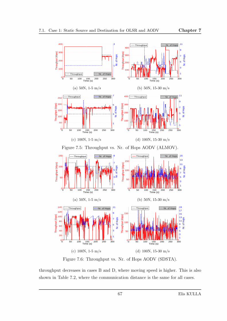
7.1. Case 1: Static Source and Destination for OLSR and AODV Chapter 7
0 50 100 150 200 250 3000
100
200
300
400
Thro
ughp
ut (k
bps)
Time (s)
1
3
Nr.
of H
ops
Throughput Nr. of Hops
(a) 50N, 1-5 m/s
0 50 100 150 200 250 3000
100
200
300
400
Thro
ughp
ut (k
bps)
Time (s)
1
3
5
7
9
11
Nr.
of H
ops
Throughput Nr. of Hops
(b) 50N, 15-30 m/s
0 50 100 150 200 250 3000
50
100
150
200
250
Thro
ughp
ut (k
bps)
Time (s)
1
3
5
7
Nr.
of H
ops
Throughput Nr. of Hops
(c) 100N, 1-5 m/s
0 50 100 150 200 250 3000
100
200
300
400
Thro
ughp
ut (k
bps)
Time (s)
1
3
5
7
9
11
Nr.
of H
ops
Throughput Nr. of Hops
(d) 100N, 15-30 m/s
Figure 7.5: Throughput vs. Nr. of Hops AODV (ALMOV).
0 50 100 150 200 250 3000
50
100
150
Thro
ughp
ut (k
bps)
Time (s)
1
3
5
7
9
Nr.
of H
ops
Throughput Nr. of Hops
(a) 50N, 1-5 m/s
0 50 100 150 200 250 3000
50
100
150
Thro
ughp
ut (k
bps)
Time (s)
1
3
5
7
9
11
13
15
Nr.
of H
ops
Throughput Nr. of Hops
(b) 50N, 15-30 m/s
0 50 100 150 200 250 3000
20
40
60
80
100
120
140
Thro
ughp
ut (k
bps)
Time (s)
1
3
5
7
9
11
Nr.
of H
ops
Throughput Nr. of Hops
(c) 100N, 1-5 m/s
0 50 100 150 200 250 3000
50
100
150
Thro
ughp
ut (k
bps)
Time (s)
1
3
5
7
9
11
13
15
17
19
Nr.
of H
ops
Throughput Nr. of Hops
(d) 100N, 15-30 m/s
Figure 7.6: Throughput vs. Nr. of Hops AODV (SDSTA).
throughput decreases in cases B and D, where moving speed is higher. This is also
shown in Table 7.2, where the communication distance is the same for all cases.
67 Elis KULLA
7.2. Case 2: Static2, Static4, Static9 Chapter 7
There are more disconnections in SDSTA scenario, as shown in Fig. 7.4, espe-
cially when the speed of movement is higher (in cases B and D), see Fig. 7.4(b) and
Fig. 7.4(d). The movement of nodes, brings dynamism to the network topology and
there are rapid changes in OLSR nodes’ routing tables. The interval of multi-casting
HELLO messages and TC messages in the network is set as default to be 2 seconds
and 5 seconds, respectively. So, the topology information is not updated on time to
keep 4 or 5-hop routes. As we can see in Fig. 7.4(a) and Fig. 7.4(c), when moving
speed is lower, the disconnections are minimized and throughput is higher.
For AODV, throughput measured in kilobits per second (kbps) versus number
of hops is shown in Fig. 7.3 and Fig. 7.4 for ALMOV and SDSTA scenarios, respec-
tively. For ALMOV scenario, in case A (Fig. 7.5(a)), both source and destination
happens to be very near, so the throughput is in its higher values, except for the
last 50 seconds when the communications occurs in 2 hops. Throughput is inversely
proportional to the number of hops. The throughput is decreased when the number
of hops is increased as shown in Table 7.1 and Table 7.2. The oscillations increase
further in SDSTA scenario, where the average number of hops is over 5.5. IN general
the performance of AODV is better than that of OLSR.
7.2 Case 2: Static2, Static4, Static9
For each scenario, we conducted simulations for 4 cases. We use UDP protocol
to transport the data from source node to destination node. The packet rate of
Constant Bit Rate (CBR) flow is 200 pps with each packet size of 230 bytes. So,
the CBR is 200pps× 230bytes/packet× 8bit/bytes = 368000bps = 368kbps.
The distance from source to destination is fixed to 848.53 meters. Taking in
consideration also the communication distance between nodes (250m), the packets
can not be delivered in less than 4 hops. However, we notice oscillations in number
of hops, which is the result of the random movement of intermediate nodes. We
think that the “route request” and “route repair” procedures of AODV cause these
oscillations, which are a common phenomenon in MANET.
In Figs. 7.7, 7.8 and 7.9, we show time domain results for three scenarios,
respectively. During 300 seconds of simulation, we show the throughput (kbps) on
the left y-axis and number of hops in the right y-axis.
68 Elis KULLA
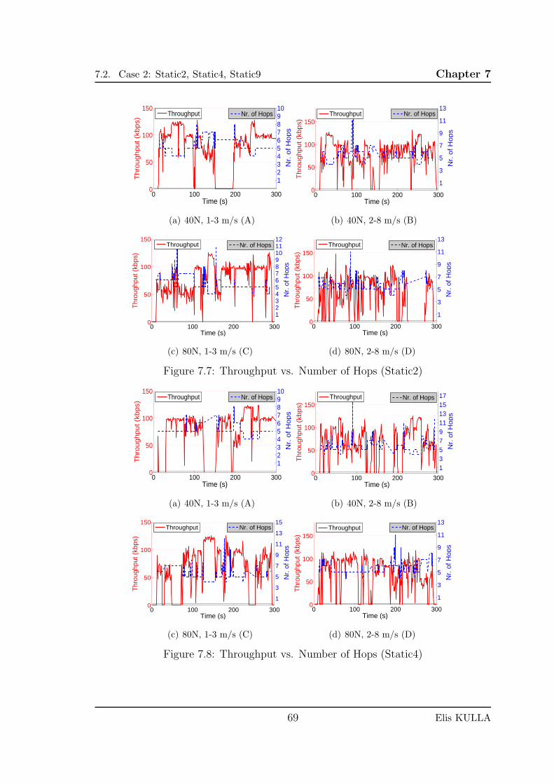
7.2. Case 2: Static2, Static4, Static9 Chapter 7
0 100 200 3000
50
100
150
Th
rou
gh
pu
t (k
bp
s)
Time (s)
12345678910
Nr.
of
Ho
ps
Throughput Nr. of Hops
(a) 40N, 1-3 m/s (A)
0 100 200 3000
50
100
150
Th
rou
gh
pu
t (k
bp
s)
Time (s)
1
3
5
7
9
11
13
Nr.
of H
op
s
Throughput Nr. of Hops
(b) 40N, 2-8 m/s (B)
0 100 200 3000
50
100
150
Thr
ough
put (
kbps
)
Time (s)
123456789101112
Nr.
of H
ops
Throughput Nr. of Hops
(c) 80N, 1-3 m/s (C)
0 100 200 3000
50
100
150
Thr
ough
put (
kbps
)
Time (s)
1
3
5
7
9
11
13
Nr.
of H
ops
Throughput Nr. of Hops
(d) 80N, 2-8 m/s (D)
Figure 7.7: Throughput vs. Number of Hops (Static2)
0 100 200 3000
50
100
150
Th
rou
gh
pu
t (k
bp
s)
Time (s)
12345678910
Nr.
of H
op
s
Throughput Nr. of Hops
(a) 40N, 1-3 m/s (A)
0 100 200 3000
50
100
150
Th
rou
gh
pu
t (k
bp
s)
Time (s)
1357911131517
Nr.
of
Ho
ps
Throughput Nr. of Hops
(b) 40N, 2-8 m/s (B)
0 100 200 3000
50
100
150
Thr
ough
put (
kbps
)
Time (s)
1
3
5
7
9
11
13
15
Nr.
of H
ops
Throughput Nr. of Hops
(c) 80N, 1-3 m/s (C)
0 100 200 3000
50
100
150
Thr
ough
put (
kbps
)
Time (s)
1
3
5
7
9
11
13
Nr.
of H
ops
Throughput Nr. of Hops
(d) 80N, 2-8 m/s (D)
Figure 7.8: Throughput vs. Number of Hops (Static4)
69 Elis KULLA
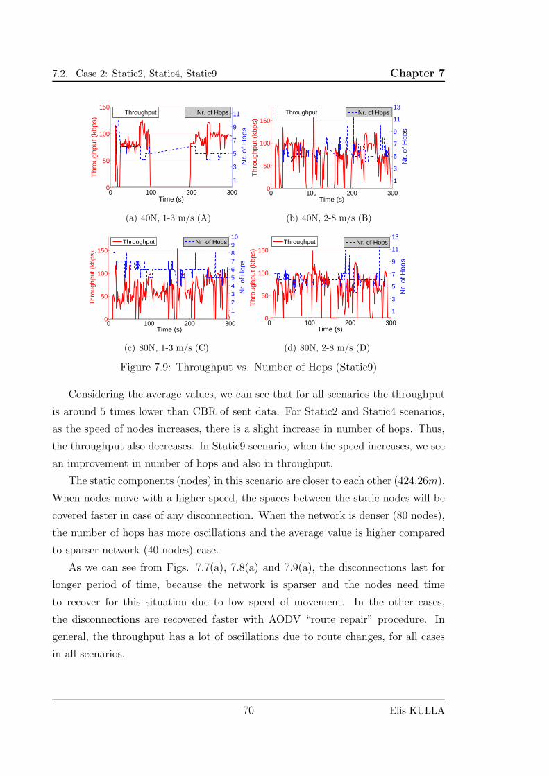
7.2. Case 2: Static2, Static4, Static9 Chapter 7
0 100 200 3000
50
100
150
Th
rou
gh
pu
t (k
bp
s)
Time (s)
1
3
5
7
9
11
Nr.
of H
op
s
Throughput Nr. of Hops
(a) 40N, 1-3 m/s (A)
0 100 200 3000
50
100
150
Thr
ough
put (
kbps
)
Time (s)
1
3
5
7
9
11
13
Nr.
of H
ops
Throughput Nr. of Hops
(b) 40N, 2-8 m/s (B)
0 100 200 3000
50
100
150
Thr
ough
put (
kbps
)
Time (s)
12345678910
Nr.
of H
ops
Throughput Nr. of Hops
(c) 80N, 1-3 m/s (C)
0 100 200 3000
50
100
150T
hrou
ghpu
t (kb
ps)
Time (s)
1
3
5
7
9
11
13
Nr.
of H
ops
Throughput Nr. of Hops
(d) 80N, 2-8 m/s (D)
Figure 7.9: Throughput vs. Number of Hops (Static9)
Considering the average values, we can see that for all scenarios the throughput
is around 5 times lower than CBR of sent data. For Static2 and Static4 scenarios,
as the speed of nodes increases, there is a slight increase in number of hops. Thus,
the throughput also decreases. In Static9 scenario, when the speed increases, we see
an improvement in number of hops and also in throughput.
The static components (nodes) in this scenario are closer to each other (424.26m).
When nodes move with a higher speed, the spaces between the static nodes will be
covered faster in case of any disconnection. When the network is denser (80 nodes),
the number of hops has more oscillations and the average value is higher compared
to sparser network (40 nodes) case.
As we can see from Figs. 7.7(a), 7.8(a) and 7.9(a), the disconnections last for
longer period of time, because the network is sparser and the nodes need time
to recover for this situation due to low speed of movement. In the other cases,
the disconnections are recovered faster with AODV “route repair” procedure. In
general, the throughput has a lot of oscillations due to route changes, for all cases
in all scenarios.
70 Elis KULLA
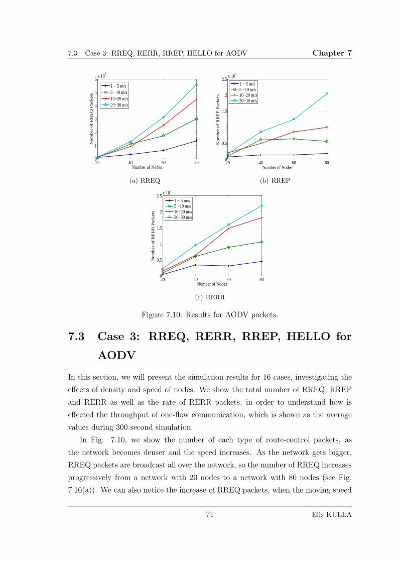
7.3. Case 3: RREQ, RERR, RREP, HELLO for AODV Chapter 7
20 40 60 800
1
2
3
4
5
6x 10
5
Number of Nodes
Num
ber
of
RR
EQ
Pac
ket
s
1 − 5 m/s5 −10 m/s10−20 m/s20−30 m/s
(a) RREQ
20 40 60 800
0.5
1
1.5
2
2.5x 10
4
Number of Nodes
Nu
mb
er o
f R
RE
P P
ack
ets
1 − 5 m/s5 −10 m/s10−20 m/s20−30 m/s
(b) RREP
20 40 60 800
0.5
1
1.5
2
2.5x 10
4
Number of Nodes
Nu
mb
er o
f R
ER
R P
ack
ets
1 − 5 m/s5 −10 m/s10−20 m/s20−30 m/s
(c) RERR
Figure 7.10: Results for AODV packets.
7.3 Case 3: RREQ, RERR, RREP, HELLO for
AODV
In this section, we will present the simulation results for 16 cases, investigating the
effects of density and speed of nodes. We show the total number of RREQ, RREP
and RERR as well as the rate of RERR packets, in order to understand how is
effected the throughput of one-flow communication, which is shown as the average
values during 300-second simulation.
In Fig. 7.10, we show the number of each type of route-control packets, as
the network becomes denser and the speed increases. As the network gets bigger,
RREQ packets are broadcast all over the network, so the number of RREQ increases
progressively from a network with 20 nodes to a network with 80 nodes (see Fig.
7.10(a)). We can also notice the increase of RREQ packets, when the moving speed
71 Elis KULLA
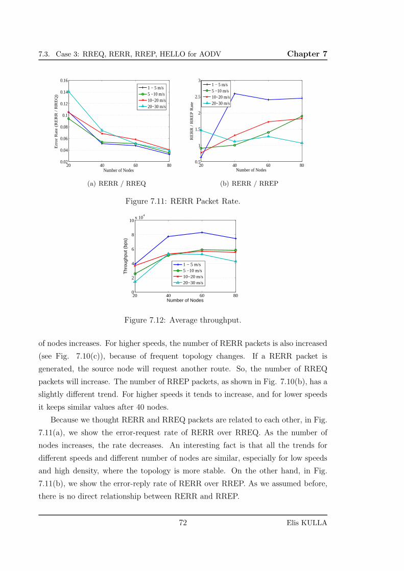
7.3. Case 3: RREQ, RERR, RREP, HELLO for AODV Chapter 7
20 40 60 800.02
0.04
0.06
0.08
0.1
0.12
0.14
0.16
Number of Nodes
Err
or
Rat
e (R
ER
R /
RR
EQ
)
1 − 5 m/s5 −10 m/s10−20 m/s20−30 m/s
(a) RERR / RREQ
20 40 60 800.5
1
1.5
2
2.5
3
Number of Nodes
RE
RR
/ R
RE
P R
ate
1 − 5 m/s5 −10 m/s10−20 m/s20−30 m/s
(b) RERR / RREP
Figure 7.11: RERR Packet Rate.
20 40 60 800
2
4
6
8
10x 10
4
Number of Nodes
Thr
ough
put (
bps)
1 − 5 m/s5 −10 m/s10−20 m/s 20−30 m/s
Figure 7.12: Average throughput.
of nodes increases. For higher speeds, the number of RERR packets is also increased
(see Fig. 7.10(c)), because of frequent topology changes. If a RERR packet is
generated, the source node will request another route. So, the number of RREQ
packets will increase. The number of RREP packets, as shown in Fig. 7.10(b), has a
slightly different trend. For higher speeds it tends to increase, and for lower speeds
it keeps similar values after 40 nodes.
Because we thought RERR and RREQ packets are related to each other, in Fig.
7.11(a), we show the error-request rate of RERR over RREQ. As the number of
nodes increases, the rate decreases. An interesting fact is that all the trends for
different speeds and different number of nodes are similar, especially for low speeds
and high density, where the topology is more stable. On the other hand, in Fig.
7.11(b), we show the error-reply rate of RERR over RREP. As we assumed before,
there is no direct relationship between RERR and RREP.
72 Elis KULLA
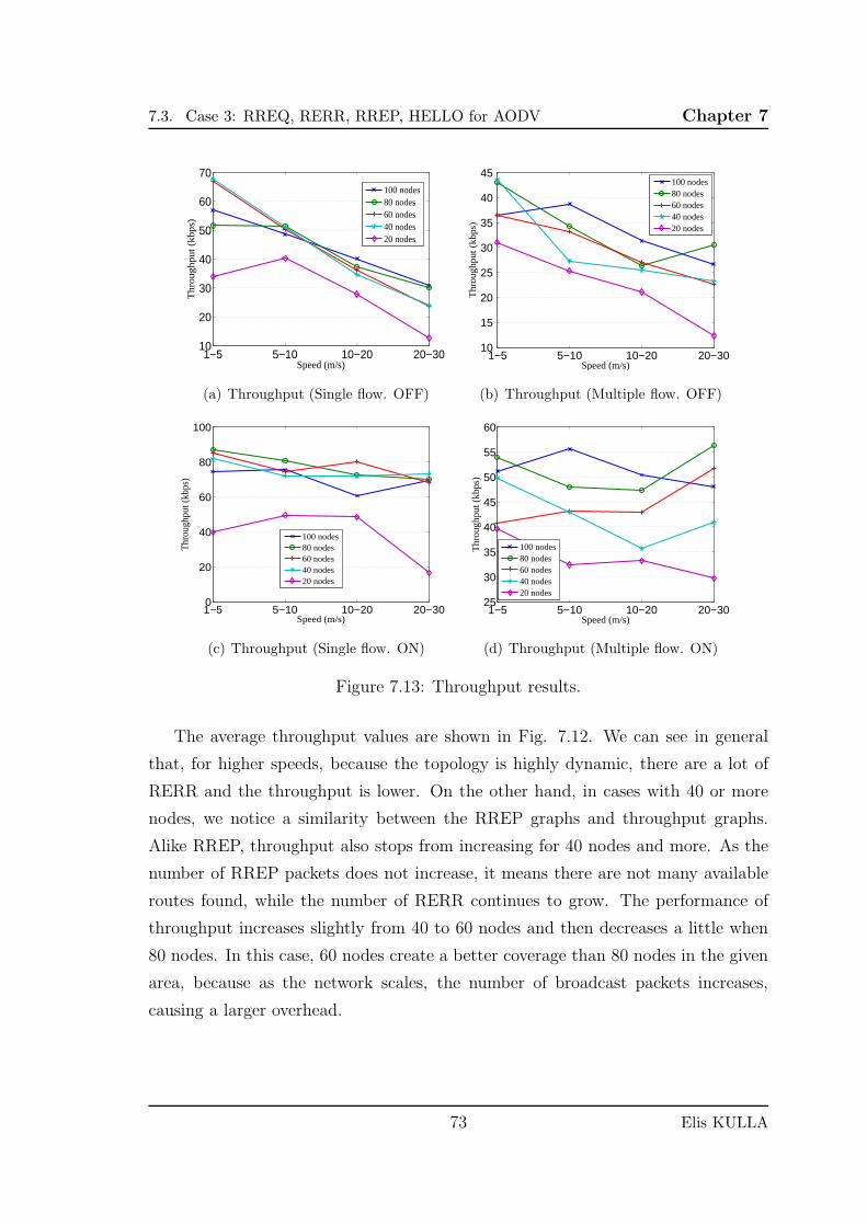
7.3. Case 3: RREQ, RERR, RREP, HELLO for AODV Chapter 7
1−5 5−10 10−20 20−3010
20
30
40
50
60
70
Speed (m/s)
Thr
ough
put
(kbp
s)
100 nodes80 nodes60 nodes40 nodes20 nodes
(a) Throughput (Single flow. OFF)
1−5 5−10 10−20 20−3010
15
20
25
30
35
40
45
Speed (m/s)
Thr
ough
put (
kbps
)
100 nodes80 nodes60 nodes40 nodes20 nodes
(b) Throughput (Multiple flow. OFF)
1−5 5−10 10−20 20−300
20
40
60
80
100
Speed (m/s)
Thr
ough
put (
kbps
)
100 nodes80 nodes60 nodes40 nodes20 nodes
(c) Throughput (Single flow. ON)
1−5 5−10 10−20 20−3025
30
35
40
45
50
55
60
Speed (m/s)
Thr
ough
put (
kbps
)
100 nodes80 nodes60 nodes40 nodes20 nodes
(d) Throughput (Multiple flow. ON)
Figure 7.13: Throughput results.
The average throughput values are shown in Fig. 7.12. We can see in general
that, for higher speeds, because the topology is highly dynamic, there are a lot of
RERR and the throughput is lower. On the other hand, in cases with 40 or more
nodes, we notice a similarity between the RREP graphs and throughput graphs.
Alike RREP, throughput also stops from increasing for 40 nodes and more. As the
number of RREP packets does not increase, it means there are not many available
routes found, while the number of RERR continues to grow. The performance of
throughput increases slightly from 40 to 60 nodes and then decreases a little when
80 nodes. In this case, 60 nodes create a better coverage than 80 nodes in the given
area, because as the network scales, the number of broadcast packets increases,
causing a larger overhead.
73 Elis KULLA
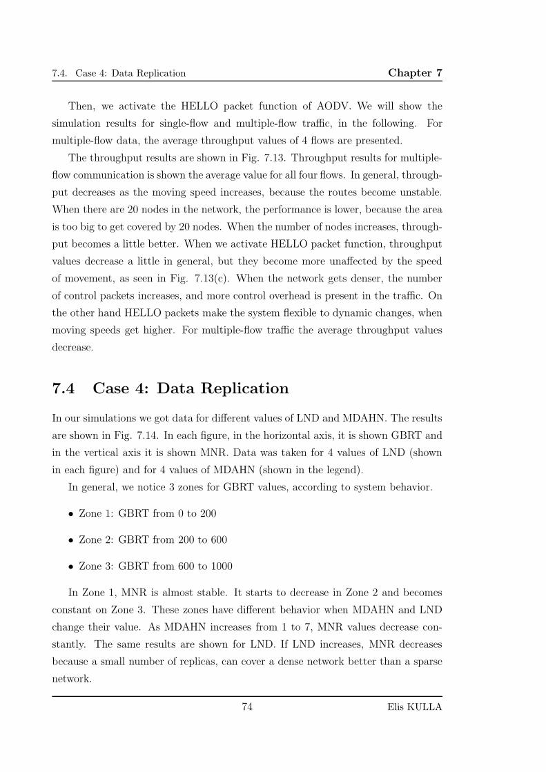
7.4. Case 4: Data Replication Chapter 7
Then, we activate the HELLO packet function of AODV. We will show the
simulation results for single-flow and multiple-flow traffic, in the following. For
multiple-flow data, the average throughput values of 4 flows are presented.
The throughput results are shown in Fig. 7.13. Throughput results for multiple-
flow communication is shown the average value for all four flows. In general, through-
put decreases as the moving speed increases, because the routes become unstable.
When there are 20 nodes in the network, the performance is lower, because the area
is too big to get covered by 20 nodes. When the number of nodes increases, through-
put becomes a little better. When we activate HELLO packet function, throughput
values decrease a little in general, but they become more unaffected by the speed
of movement, as seen in Fig. 7.13(c). When the network gets denser, the number
of control packets increases, and more control overhead is present in the traffic. On
the other hand HELLO packets make the system flexible to dynamic changes, when
moving speeds get higher. For multiple-flow traffic the average throughput values
decrease.
7.4 Case 4: Data Replication
In our simulations we got data for different values of LND and MDAHN. The results
are shown in Fig. 7.14. In each figure, in the horizontal axis, it is shown GBRT and
in the vertical axis it is shown MNR. Data was taken for 4 values of LND (shown
in each figure) and for 4 values of MDAHN (shown in the legend).
In general, we notice 3 zones for GBRT values, according to system behavior.
• Zone 1: GBRT from 0 to 200
• Zone 2: GBRT from 200 to 600
• Zone 3: GBRT from 600 to 1000
In Zone 1, MNR is almost stable. It starts to decrease in Zone 2 and becomes
constant on Zone 3. These zones have different behavior when MDAHN and LND
change their value. As MDAHN increases from 1 to 7, MNR values decrease con-
stantly. The same results are shown for LND. If LND increases, MNR decreases
because a small number of replicas, can cover a dense network better than a sparse
network.
74 Elis KULLA
7.4. Case 4: Data Replication Chapter 7
0 200 400 600 800 10000
20
40
60
80
100
GBRT
MN
R
LND=1
MDAHN=1MDAHN=3MDAHN=5MDAHN=7
(a)
0 200 400 600 800 10000
20
40
60
80
100
GBRT
MN
R
LND=3
MDAHN=1MDAHN=3MDAHN=5MDAHN=7
(b)
0 200 400 600 800 10000
20
40
60
80
100
GBRT
MN
R
LND=5
MDAHN=1MDAHN=3MDAHN=5MDAHN=7
(c)
0 200 400 600 800 10000
20
40
60
80
100
GBRT
MN
R
LND=7
MDAHN=1MDAHN=3MDAHN=5MDAHN=7
(d)
Figure 7.14: FDRM system results.
For plot lines of MDAHN 1 and 3, we notice that there is a similar trend for Zone
1. This means that, for low values of MDAHN (less than 3), the system requires a
lot of replicas in order to satisfy the QoS requirements.
From 400 to 1000 ms of GBRT, the plot lines of MDAHN 5 and 7, have similar
trends and MNR have similar values. In this case, where the system requires higher
GBRT and MDAHN is more than 5, the number of replicas is low, because they
should be enough to satisfy these QoS requirements.
75 Elis KULLA

Chapter 8
Conclusions and Future Works
8.1 Conclusions
In this work, we designed and implemented a MANET testbed, in which we im-
plemented three cases in different environments and topologies. In the first case,
we use our indoor stairs environment to implement 2 scenarios (VS and VM). We
implement 3 other scenarios in our outdoor bridge environment (OBST, OBSM and
OBDM). And we use MAC filtering to create linear and mesh topologies in order to
test multimedia traffic data in indoor environment. We used throughput, delay and
packetloss as metrics for performance assessment of OLSR, AODV and BATMAN
routing protocols.
We also implemented a simulation system for testing MANETs, based on NS2
simulator. We considered four simulation cases for different applications of MANETs.
In the first case, static source and destination are taken in consideration with two
scenarios (ALMOV and SDSTA) In the second case, we increase the number of static
nodes in the network, comparing three scenarios (static2, static4 and static9). The
third case is concentrated on the performance of AODV, regarding control packets.
Finally, a QoS Data Replication framework is presented in the fourth case.
In the following are shown the conclusions.
77
8.1. Conclusions Chapter 8
8.1.1 Experiments
8.1.1.1 Case 1
• Both protocols show a good performance in both STAS and SHIS scenario, for
one-hop and two-hop communications.
• For 3 or 4 hops from source (node 4 and 5, respectively), the throughput
decreased about 50% compared with DTR, regarding STAS scenario.
• In case of SHIS scenario, when destination was node 4 or node 5, the through-
put decreased about 60% compared with DTR.
• Delay is increased after three hops for STAS scenario and after two hops for
SHIS scenario.
• In general, OLSR protocol showed better performance than BATMAN proto-
col.
• The throughput of BATMAN is better than OLSR for SHIS scenario. BAT-
MAN buffers the packets when routes are unstable. However, the buffering
increases the delay.
• Regarding 1 → 5 flow, in SHIS scenario, source and destination nodes were
closer to each other, so the throughput was higher compared with 1 → 5 in
STAS scenario.
8.1.1.2 Case 2
• The movement of the nodes, did not bring any disconnection in the first hop of
the communication. The throughput was almost same as DTR and packetloss
was almost 0, for all three scenarios.
• When the destination is in the third floor or higher, there are oscillations for
both throughput and packetloss, caused by the increased number of hops that
the packets had to use to reach the destination.
78 Elis KULLA
8.1. Conclusions Chapter 8
• When the data flows through 3 or 4 hops to destination, the throughput de-
creases to less than half of the sent DTR and the packetloss increases to no-
ticeable values. Communication for three or more hops in a MANET testbed
becomes difficult.
8.1.1.3 Case 3
• For audio transmissions, the performance was almost the same for both LT
and MT topologies. The throughput had a few oscillations.
• The average delay values were under 20 ms and 10 ms, for LT and MT, re-
spectively.
• Packetloss is less than 1 pps for all cases of audio data.
• For video transmissions with higher data rates, the performance decreased as
the number of hops increases up to 4 hops in 1 → 5 flow.
• For MT, we could see that the performance for 1 → 2, 1 → 3 and 1 → 4 flows
were almost similar, while in case of 1 → 5 flow, the values of throughput fell
to around 20kbps.
• We could see that for audio data there is no difference between LT and MT,
but for video data, in MT case the average value of throughput decreased and
its oscillations increased.
• The packetloss, is closely related to throughput so it had a similar behavior.
• In LT scheme, routes are static. While in MT scheme, routes change and this
decreased throughput and increased packetloss.
• Delay values were higher in the case of LT scheme because of more number of
hops.
8.1.2 Simulations
8.1.2.1 Case 1
• When the distance between source and destination is a random function, we
can understand the effects of mobility model.
79 Elis KULLA
8.1. Conclusions Chapter 8
• There are disconnections when there are 4 or more number of hops.
• When moving speed is higher, the topology is more dynamic and the topology
information is not updated in time throughout all nodes.
• When the distance between source and destination is a random function, we
can understand the effects of mobility model.
• When moving speed is higher, there are more RERRs for AODV nodes. The
“Local repair” and new “route request” procedures find different routes, which
results in more oscillations in the number of hops and throughput.
• When the node density is high, there are more oscillations.
• The number of hops and throughput are inverse proportional for AODV rout-
ing protocol.
8.1.2.2 Case 2
• When the distance between source and destination is fixed, we can understand
the effects of mobility model and routing protocol.
• For all scenarios, the average throughput is around 5 times lower than CBR
of sent data.
• In Static2 and Static4 scenarios, the performance decreases with the increase
of the speed, while in Static9 scenario the performance increases when the
speed is increased.
• The number of hops is higher and has more oscillations for denser networks
(80 nodes).
8.1.2.3 Case 3
• The movement of the nodes, did not bring any disconnection in the first hop of
the communication. The throughput was almost same as DTR and packetloss
was almost 0, for all three scenarios.
80 Elis KULLA
8.1. Conclusions Chapter 8
• When the destination is in the third floor or higher, there are oscillations for
both throughput and packetloss, caused by the increased number of hops that
the packets had to use to reach the destination.
• When the data flows through 3 or 4 hops to destination, the throughput de-
creases to less than half of the sent DTR and the packetloss increases to no-
ticeable values. Communication for three or more hops in a MANET testbed
becomes difficult.
• When HELLO function is off, the number of RERR packets increases when
the number of nodes in the network increases. The number of RERR packets
increases in multi-flow traffic case. As the speed of nodes increases, there are
more RERR packets in the network for both single-flow and multi-flow cases.
The number of RERR packets increases for multiple-flow traffic in the network.
• In general, throughput decreases as the moving speed increases. When there
are 20 nodes in the network, the performance is lower, because the area cov-
erage is lower. When the number of nodes increases, throughput improves,
for 40 or more nodes. In the case of multi-flow communication the average
throughput is lower than the single-flow case.
• The number of HELLO packets in the network is the same for both single-flow
and multiple-flow traffic. It is also not affected by speed, but it increases when
the number of nodes in the network increases.
• When HELLO function is on, the number of RERR packets decreases.
• Throughput values decrease a little in general, but they become more unaf-
fected by the speed of movement, being helped by HELLO packets information.
8.1.2.4 Case 4
From our MATLAB simulations, we got the following conclusions:
• There are 3 different zones for GBRT values.
• As LND and MDAHN increase, MNR decreases.
• In Zone 1 for MDAHN 1 and 3, the values of MNR are similar.
• In Zone 2 and 3 for MDAHN 5 and 7, the values of MNR are similar and low.
81 Elis KULLA
8.2. Future Works Chapter 8
8.2 Future Works
In the following are shown some future aspects of MANETs, which can be inspired
by this work.
Testbed Improvement: This work inspires us to improve our testbed with more
nodes and spread our experiments in outdoor environment and all over the
campus. We would also like to create a monitoring interface, in order to have
access to real-time results and accurate node positions. Moreover, an accu-
rate moving mechanism is important to create the same topology in different
experimental settings.
Simulated Mobility: During simulation, the mobility model used for node move-
ment has a key influence on the performance of different protocols and algo-
rithms. We would like to create more realistic mobility models, similar to real
life cities, campuses or buildings.
Applications of MANET: MANET will be the next technology for creating cheap
and autonomous backbones of modern networks. We want to implement the
use of MANETs in airspace communications (Air2air network) and in Smart
Cities (Internet of Things).
82 Elis KULLA
References
[1] H. Lundgren, E. Nordstrom, C. Tschudin, “Coping with Communication Gray
Zones in IEEE 802.11b based Ad hoc Networks”, Proc. of WoWMoM ‘02, pp.
49-55, 2002.
[2] L. Barolli, M. Ikeda, G. De Marco, A. Durresi and F. Xhafa, “Performance
Analysis of OLSR and BATMAN Protocols Considering Link Quality Param-
eter”, Proc. of International Conference on Advanced Information Networking
and Applications (AINA-2009), pp. 307-314, May 2009.
[3] G. De Marco, M. Ikeda, T. Yang and L. Barolli, “Experimental Performance
Evaluation of a Pro-active Ad-hoc Routing Protocol in Outdoor and Indoor
Scenarios”, Proc. of International Conference on Advanced Information Net-
working and Applications (AINA-2007), pp. 7-14, May 2007.
[4] M. Ikeda, L. Barolli, M. Hiyama, T. Yang, G. De Marco and A. Durresi, “Per-
formance Evaluation of a MANET Testbed for Differenet Topologies,” Proc.
of International Conference on Network-Based Information Systems (NBiS-
2009), Indianapolis, pp. 327-334, August 2009.
[5] E. Kulla, M. Ikeda, L. Barolli and R. Miho, “Impact of Source and Destina-
tion Movement on MANET Performance Considering BATMAN and AODV
Protocols“, Proc. of International Conference on Broadband, Wireless Com-
puting, Communication and Applications (BWCCA-2010), pp. 94-101, 2010.
[6] D.A. Maltz, J. Broch, D.B. Johnson, “Quantitative Lessons From a Full-Scale
Multi-Hop Wireless Ad Hoc Network Testbed”, IEEE Personal Communica-
tions, Vol. 8, pp. 8-15, 2001.
[7] R.S. Gray, D. Koltz, “Outdoor Experimental Comparison of Four Ad Hoc
Routing Algorithms”, Proc. of MSWiM ‘04, Vol. 1, pp. 1-7, 2004.
83
References
[8] G. Anastasi, E. Borgia, M. Conti, E. Gregori, “IEEE 802.11b Ad Hoc Net-
works: Performance Measurements”, Cluster Computing, Vol. 8, pp. 135-145,
2005.
[9] V. Kawadia, P.R. Kumar, “Experimental Investigations into TCP Perfor-
mance over Wireless Multihop Networks”, Proc. of ACM SIGCOMM E-WIND
’05, pp. 29-34, 2005.
[10] T.H. Clausen, G. Hansen, L. Christensen, G.Behrmann, “The Optimized Link
State Routing Protocol Evaluation through Experiments and Simulation”,
Proc. of Wireless Personal Multimedia Communications, PhD’s Thesis, Aal-
borg University, 2001.
[11] D. Johnson, G. Hancke, “Comparison of two Routing Metrics in OLSR on a
Grid Based Mesh Network”, Ad Hoc Network., Elsevier Science Publishers B.
V., 2009, 7, 374-387.
[12] C. Tschudin, P. Gunningberg, H. Lundgren, E. Nordstrom, “Lessons from
Experimental MANET Research”, Ad Hoc Network, Vol. 3, No. 2, pp. 221-
233, 2005.
[13] E. Nordstrom, “APE - A Large Scale Ad-hoc Network Testbed for Repro-
ducible Performance Tests”, Master’s thesis, Uppsala University, 2002.
[14] Y. Owada, Y. Takahashi, T. Suda, H. Terui, F. Taki, T. Yagi, K. Mase,
“A Large Scale Wireless Mobile Ad-hoc Network Testbed”, Proc. of IEEE
Vehicular Technology Conference, pp. 324-328, September 2005.
[15] R. Draves, J. Padhye, and B. Zill, “Comparison of Routing Metrics for Static
Multi-hop Wireless Networks”, Proc. of International Conference on Spe-
cial Interest Group on Data Communication (SIGCOMM-2004), pp. 133-144,
2004.
[16] J. Bicket, D. Aguayo, S. Biswas, and R. Morris, “Architecture and Evaluation
of an Unplanned 802.11b Mesh Network”, Proc. of International Conference
on Mobile Computing and Networking (MOBICOM-2005), pp. 31-42, 2005.
84 Elis KULLA
References
[17] D. A. Maltz, J. Broch, and D. B. Johnson, “Lessons from a Full-scale Multihop
Wireless Ad-Hoc Network Testbed”, Journal on Personal Communications,
Vol. 8, No. 1, pp. 8-15, February 2001.
[18] D. B. Johnson, D. A. Maltz, and J. Broch, “DSR: The Dynamic Source Rout-
ing Protocol for Multi-Hop Wireless Ad-Hoc Networks”, Journal on Ad-Hoc
Networking, Chap. 5, pp. 139-172, 2001.
[19] R. S. Gray, D. Kotz, C. Newport, N. Dubrovsky, A. Fiske, J. Liu, C. Masone, S.
McGrath and Y. Yuan, “Outdoor Experimental Comparison of Four Ad-Hoc
Routing Algorithms”, Proc. of Modeling, Analysis and Simulation of Wireless
Mobile Systems (MSWiM-2004), pp. 220-229, 2004.
[20] E. Borgia, M. Conti, and E. Gregori, “IEEE 802.11b Ad-Hoc Networks: Per-
formance Measurements”, Journal of Cluster Computing, Vol. 8, No. 2-3, pp.
135-145, 2005.
[21] T. Clausen, G. Hansen, L. Christensen, and G. Behrmann, “The Optimized
Link State Routing Protocol, Evaluation through Experiments and Simula-
tion”, Proc. of IEEE Symposium on Wireless Personal Mobile Communi-
cations, Available online at http://hipercom.inria.fr/olsr/wpmc01.ps,
September 2001.
[22] D. Johnson and G. Hancke, “Comparison of Two Routing Metrics in OLSR
on a Grid based Mesh Network”, Journal on Ad-Hoc Networks, Vol. 7, No. 2,
pp. 374-387, March 2009.
[23] G. De Marco, M. Ikeda, T. Yang and L. Barolli, “Experimental Performance
Evaluation of a Proactive Ad-hoc Routing Protocol in Outdoor and Indoor
Scenarios”, Proc. of AINA-2007, pp. 7-14, May 2007.
[24] A. M. Hanashi, A. Siddique, I. Awan, and M. Woodward, “Performance Eval-
uation of Dynamic Probablilistic Flooding Under Different Mobility Models
in MANETs”, Proc. of International Conference on Parallel and Distributed
Systems (ICPADS-2007), Vol. 2, pp. 1-6, December 2007.
[25] A. M. Hanashi, I. Awan, and M. Woodward, “Performance Evaluation with
Different Mobility Models for Dynamic Probabilistic Flooding in MANETs”,
85 Elis KULLA
References
Journal on Mobile Information Systems (IJMIS), Vol. 5, No. 1, pp. 65-80,
2009.
[26] Andres L. Cavilla, Gerard Baron, Thomas E. Hart, Lionel Litty and Eyal
de Lara, “Simplified Simulation Models for Indoor MANET Evaluation are
not Robust”, Proc. of Annual IEEE Communications Society SECON-2004
Conference, pp. 610-620, October 2004.
[27] Aarti Munjal, Tracy Camp, William C. Navidi, “Constructing Rigorous
MANET Simulation Scenarios with Realistic Mobility”, Proc. of European
Wireless (EW-2010) Conference, pp. 817-824, April 2010.
[28] P. Santi, “Topology Control in Wireless Ad Hoc and Sensor Networks”, Wiley,
2005.
[29] One Laptop Per Child project. http://www.laptop.org/en/.
[30] M. Abolhasan, T. Wysocki, E. Dutkiewicz, “A Review of Routing Protocols
for Mobile Ad hoc Networks” Ad Hoc Networks, Vol. 2, No. 1, pp. 1-22, 2004.
[31] L. Barolli, M. Ikeda, G.D. Marco, A. Durresi, F. Xhafa, “Performance Analy-
sis of OLSR and BATMAN Protocols Considering Link Quality Parameter”,
Proc. of International Conference on Advanced Information Networking and
Application, IEEE Computer Society, pp. 307-314, 2009.
[32] T. Clausen, P. Jacquet, “Optimized Link State Routing Protocol”, Technical
report, Project Hipercom, INRIA Rocquencourt, France, 2003.
[33] A. Neuman, C. Aichele, M. Lindner, M. Wunderlich, “Better Approach To
Mobile Ad-hoc Networking (B.A.T.M.A.N)”, Work in Progress, 2008.
[34] Zygmunt J. Haas, Joseph Y. Halpern, and Li Li, “Gossip-based ad hoc rout-
ing”, IEEE/ACM Transactions Networking, Vol. 14, No. 3, pp. 479-491, 2006.
[35] C. Perkins, E. Belding-Royer, and S. Das, “Ad hoc On-Demand Distance
Vector(AODV) Routing, RFC3561”, Technical report, Nokia Research Center,
University of California, University of Cincinnati, 2003.
86 Elis KULLA
References
[36] S. Sanghani, T.X. Brown, S. Bhandare, S. Doshi, “EWANT: The Emulated
Wireless Adhoc Testbed”, Proc. of IEEE WCNC–2003, pp. 1884–1849, March
2003.
[37] L. Rizzo, “Dummynet: A Simple Approach to the Evaluation of Network
Protocols”, Journal of Computer Communication Review, Vol. 27, No. 1, pp.
31–41, 1997.
[38] T. Camp, J. Boleng, V. Davies, “A Survey of Mobility Models for Ad Hoc Net-
work Research”, Journal of Wireless Communications and Mobile Computing,
Vol. 2, No. 5, pp. 483–502, 2002.
[39] J. Bicket, D. Aguayo, S. Biswas, R. Morris, “Architecture and Evaluation of
an Unplanned 802.11b Mesh Network”, Proc. of MOBICOM–2005, pp. 31–42,
2005.
[40] L. Barolli, M. Ikeda, F. Xhafa, A. Durresi, “A testbed for MANETs: Imple-
mentation Experiences and Learned Lessons”, IEEE Systems Juornal, Vol. 4,
No. 2, pp. 243–252, June 2010.
[41] D. Johnson, T. Stack, R. Fish, D. Flickinger, R. Ricci, J. Lepreau, “TrueMo-
bile: A Mobile Robotic Wireless and Sensor Network Testbed, Flux Technical
Note FTN-2005-02” Proc. of 25-th Annual Joint Conference of the IEEE Com-
puter and Communications Societies, 2006.
[42] D.A. Maltz, J. Broch, D.B. Johnson, “Lessons from a Full–scale Multihop
Wireless Ad-Hoc Network Testbed”, Journal on Personal Communications,
Vol. 8, No. 1, pp. 8–15, February 2001.
[43] R.S. Gray, D. Kotz, C.C. Newport, N. Dubrovsky, A. Fiske, J. Liu, C. Masone,
S. McGrath, Y. Yuan, “Outdoor Experimental Comparison of Four Ad hoc
Routing Algorithms” Proc. of MSWiM–2004, pp. 220–229, 2004.
[44] D. Raychaudhuri, I. Seskar, M. Ott, S. Ganu, K. Ramachandran, H. Kremo,
R. Siracusa, H. Liuand, M. Singh, “Overview of ORBIT Radio Grid Testbed
Evaluation of Next-generation Wireless Network Protocols”, Proc. of IEEE
WCNC–2005, pp. 1664–1669, March 2005.
87 Elis KULLA
References
[45] Rt2x00 Project for Linux Wireless Cards Drivers, Available Online at:
http://rt2x00.serialmonkey.com/.
[46] Ralink RT2570 USB Enhanced Driver, Available Online at:
http://homepages.tu-darmstadt.de/~p_larbig/wlan/.
[47] A. Dainotti, A. Botta, and A. Pescap, “Do you know what you are generat-
ing?” Proc. of International Conference on emerging Networking EXperiments
and Technologies (CoNEXT-2007), New York, NY, USA, pp. 1-2, 2007.
[48] F. Hillebrand, “GSM and UMTS: The Creation of Global Mobile Communi-
cation”, Chichester [u.a.] Wiley, 2002.
[49] R. E. Shannon, “Introduction to the Art and Science of Simulation”, Proc. of
the 30th Conference on Winter Simulation (WSC ’98), 1998.
[50] “NETSIM - The Cisco Network Simulator & Router Simulator”, Available on-
line at http://www.boson.com/netsim-cisco-network-simulator, Accessed on
March 2012.
[51] “OPNET - Optimized Network Engineering Tools”, Available online at
http://www.opnet.com/, Accessed on March 2012.
[52] “NS2 - Network Simulator version 2”, Available online at
http://www.isi.edu/nsnam/ns/, Accessed on March 2012.
[53] “NS3 - Network Simulator version 3”, Available online at
http://www.nsnam.org/, Accessed on March 2012.
[54] J. Broch, D. A. Maltz, D. B. Johnson, Y.-C. Hu, and J. Jetcheva, “A Perfor-
mance Comparison of Mmulti-hop Wireless Ad hoc Network Routing Proto-
cols”, Proceedings of the Fourth Annual ACM/IEEE International Conference
on Mobile Computing and Networking (Mobicom-98), ACM, October 1998.
[55] S. Sathya, S. Kuppuswami, R. Ragupathi, “Replication Strategies for Data
Grids”, Proc. of International Conference on Advanced Computing and Com-
munications (ADCOM-2006), pp. 123-128, December 2006, doi: 10.1109/AD-
COM.2006.4289868.
88 Elis KULLA
References
[56] X. Sun, J. Zheng, Q. Liu, Y. Liu, “Dynamic Data Replication Based on Access
Cost in Distributed Systems” Proc. of Fourth International Conference on
Computer Sciences and Convergence Information Technology (ICCIT-2009),
pp. 829-834, November 2009, doi: 10.1109/ICCIT.2009.198.
[57] V. Andronikou, K. Mamouras, K. Tserpes, D. Kyriazis, T. Varvarigou, “Dy-
namic QoS-aware Data Replication in Grid Environments Based on Data Im-
portance”, Future Generation Computer Systems, Vol. 28, No. 3, pp. 544-553,
March 2012, ISSN 0167-739X, doi: 10.1016/j.future.2011.02.003.
[58] P. Gupta and P. Kumar, “The Capacity of Wireless Networks”, IEEE Trans-
actions on Information Theory, Vol. 46, No. 2, pp. 388404, March 2000.
[59] V. Iyer, A. Pruteanu, S. Dulman, “NetDetect: Neighborhood Discovery in
Wireless Networks Using Adaptive Beacons”, Proc. of Fifth IEEE Interna-
tional Conference on Self-Adaptive and Self-Organizing Systems 2011 (SASO-
2011), pp. 31-40, October 2011, doi: 10.1109/SASO.2011.14.
[60] Y. Mansouri, R. Monsefi, “Optimal Number of Replicas with QoS Assur-
ance in Data Grid Environment”, Proc. of Second Asia International Confer-
ence on Modeling & Simulation (AICMS-2008), pp. 168-173, May 2008, doi:
10.1109/AMS.2008.147.
[61] J. M. Mendel, “Fuzzy Logic Systems for Engineering: A Tutorial”, Proc. of
Journal the IEEE, Vol. 83, No. 3, pp. 345-377, March 1995.
[62] E. Chissungo, E. Blake, H. Le, “Investigation into Batman-adv Protocol
Performance in an Indoor Mesh Potato Testbed”, Proc. of IEEE Interna-
tional Conference on Intelligent Networking and Collaborative Systems (IEEE
INCoS-2011), pp. 8-13, 2011.
[63] E. Kulla, M. Ikeda, L. Barolli and R. Miho, “Impact of Source and Destina-
tion Movement on MANET Performance Considering BATMAN and AODV
Protocols“, Proc. of International Conference on Broadband, Wireless Com-
puting, Communication and Applications (BWCCA-2010), pp. 94-101, 2010.
89 Elis KULLA
References
[64] “UM-OLSR, GNU General Public License version 2.0 (GPLv2)”, Available
online at http://sourceforge.net/projects/um-olsr/develop. Accessed on April
2012.
[65] Kiess, W., and Mauve, M.: A Survey on Real-world Implementations of Mobile
Ad–hoc Networks. J. Ad-Hoc Networks, Vol. 5, No. 3, pp. 324–339, 2007.
[66] Lundgren, H., Nordstrom, E. and Tschudin, C.: Coping with Communica-
tion Gray Zones in IEEE 802.11b Based Ad-Hoc Networks. In: WOWMOM–
2002/MOBICOM–2002, pp. 49–55, 2002.
[67] A. Tonnesen, “OLSRd: Implementation Code of the OLSR”, Available on line
at http://www.olsr.org/.
[68] T. Clausen and P. Jacquet, “Optimized Link State Routing Protocol (OLSR)”,
RFC 3626 (Experimental), 2003.
[69] D. S. J. D. Couto, D. Aguayo, J. Bicket, and R. Morris, “A High Throughput
Path Metric for Multi-hop Wireless Routing”, Proc. of MobiCom-2003, pp.
134-146, 2003.
[70] R. Li, R. Yang, D. Hu, “A designing of Mobility Management Mechanism
in MANET in Disaster-Rescue Situations”, Proc. of 11th IEEE International
Conference on Communication Technology 2008 (ICCT-2008), pp. 596-599,
November 2008, doi: 10.1109/ICCT.2008.4716140.
[71] F. Xhafa, E. Asimakopoulou, N. Bessis, L. Barolli, M. Takizawa, “An Event-
based Approach to Supporting Team Coordination and Decision Making in
Disaster Management Scenarios”, Proc. of Third International Conference on
Intelligent Networking and Collaborative Systems (INCoS 2011), pp. 741-745,
Fukuoka, Japan November-December 2011.
[72] M. Pichler, T. Hofer, G. Leonhartsberger, “Considerations and Requirements
for Tools Supporting Mobile Teams” Proc. of International Conference on
Distributed Computing Systems Workshops 2002, pp. 389- 390, 2002, doi:
10.1109/ICDCSW.2002.1030800.
90 Elis KULLA
References
[73] G. Yuan, X. Zhang, Q. Yao, K. Wang, “Hierarchical and Modular Surveil-
lance Systems in ITS”, IEEE Intelligent Systems, Vol. 26, No. 5, pp. 10-15,
September-October 2011, doi: 10.1109/MIS.2011.88.
[74] S.L. Toral, D. Gregor, M. Vargas, F. Barrero, F. Cortes, “Distributed Ur-
ban Traffic Applications Based on CORBA Event Services”, Int. J. of Space-
Based and Situated Computing, Vol. 1, No. 1, pp. 86 - 97, 2011, doi:
10.1504/IJSSC.2011.039110.
[75] Youtube, http://www.youtube.com/
[76] F. Thouin, M. Coates, “Video-on-Demand Networks: Design Approaches and
Future Challenges”, IEEE Network, Vol. 21, No. 2, pp. 42-48, March-April
2007, doi: 10.1109/MNET.2007.334311.
[77] E. Vasilyeva, M. Pechenizkiy, S. Puuronen, “Towards the Framework of
Adaptive User Interfaces for eHealth”, Proc. of 18th IEEE Symposium on
Computer-Based Medical Systems 2005 (CBMS-2005), pp. 139-144, June 2005,
doi: 10.1109/CBMS.2005.101.
[78] T. Hara, “Data Replication Issues in Mobile Ad hoc Networks”, Proc. of Six-
teenth International Workshop on Database and Expert Systems Applications
2005, pp. 753-757, August 2005, doi: 10.1109/DEXA.2005.70.
[79] E. Atsan, O. Ozkasap, “Applicability of Eigenvector Centrality Principle to
Data Replication in MANETs”, Proc. of 22nd International Symposium on
Computer and Information Sciences (ISCIS-2007), pp. 1-6, November 2007,
doi: 10.1109/ISCIS.2007.4456889.
[80] P. Pabmanabhan, L. Gruenwald, “DREAM: A Data Replication Technique for
Real-Time Mobile Ad-hoc Network Databases”, Proc. of 22nd International
Conference on Data Engineering 2006 (ICDE-06), pp. 134, April 2006, doi:
10.1109/ICDE.2006.52.
[81] V. Martins, E. Pacitti, P. Valduriez, “Survey of Data Repli-
cation in P2P Systems”, Technical Report, 2006. Online at
http://hal.inria.fr/inria-00122282/, Accessed on July 10, 2012.
91 Elis KULLA
References
[82] C. Coulon , E. Pacitti , P. Valduriez, “Consistency Management for Partial
Replication in a High Performance Database Cluster”, Proc. of the 11th In-
ternational Conference on Parallel and Distributed Systems (ICPADS-05), pp.
809-815, 2005.
[83] P. A. Bernstein, V. Hadzilacos, N. Goodman, “Concurrency Control and Re-
covery in Database Systems”, Published by Adison-Wesley, 1987, ISBN: 0-
201-10715-5.
[84] B. Kemme, G. Alonso, “A New Approach to Developing and Implementing
Eager Database Replication Protocols”, ACM Transactions on Database Sys-
tems, Vol. 25, No. 3, pp. 333-379, 2000.
[85] E. Pacitti, P. Minet, and E. Simon, “Fast Algorithms for Maintaining Replica
Consistency in Lazy Master Replicated Databases”, Proc. of the 25th Interna-
tional Conference on Very Large Data Bases (VLDB-99), pp. 126-137, 1999.
[86] Y. Saito and M. Shapiro, “Optimistic Replication”, ACM Computing Surveys,
Vol. 37, No. 1, pp. 42-81, 2005.
[87] L. A. Zadeh, “Fuzzy Logic, Neural Networks, and Soft Computing”, Commu-
nications ACM (92pp), pp. 77-84, March 1994.
[88] B. I. Bondarev, A. P. Durkin, A. D. Ovsvannikov, “New mathematical Opti-
mization Models for RFQ Structures”, Proc. of the Particle Accelerator Con-
ference 1999, pp. 2808-2810, 1999, doi: 10.1109/PAC.1999.792945.
[89] Z.Huanjiong, “Research a New Method of Search Engine Optimization”, Proc.
of 2010 International Conference on Internet Technology and Applications,
pp.1-3, August 2010, doi: 10.1109/ITAPP.2010.5566137.
[90] F. He, W. Chen, “Stochastic Optimization Problem through Particle Swarm
Optimization Algorithm”, Proc. of International Conference on Networks Se-
curity, Wireless Communications and Trusted Computing (NSWCTC-2009),
pp. 692-695, April 2009, doi: 10.1109/NSWCTC.2009.355.
92 Elis KULLA
References
[91] T. Kanungo, D. M. Mount, N. S. Netanyahu, C. D. Piatko, R. Silverman,
A. Y. Wu, “An Efficient k-means Clustering Algorithm: Analysis and Imple-
mentation”, IEEE Transactions on Pattern Analysis and Machine Intelligence,
Vol. 24, No. 7, pp. 881-892, July 2002, doi: 10.1109/TPAMI.2002.1017616.
[92] E. J. Candes, T. Tao, “Decoding by Linear Programming”, IEEE Transactions
on Information Theory, , Vol. 51, No. 12, pp. 4203-4215, December 2005, doi:
10.1109/TIT.2005.858979.
93 Elis KULLA

List of Papers
Journal Papers
1. E. Kulla, M. Hiyama, M. Ikeda, L. Barolli, V. Kolici, R. Miho, “MANET
Performance for Source and Destination Moving Scenarios Considering OLSR
and AODV Protocols”, Mobile Information Systems (MIS), Vol. 6, No. 4, pp.
325-329, doi: 10.3233/MIS-2010-0106, 2010.
2. E. Kulla, M. Hiyama, M. Ikeda, L. Barolli, “Performance Comparison of OLSR
and BATMAN Routing Protocols by a MANET Testbed in Stairs Environ-
ment”, International Journal of Computers & Mathematics with Applications
(IJCAMWA), Vol. 63, No. 2, pp. 339-349, doi: 10.1016/j.camwa.2011.07.035,
January 2012.
3. E. Kulla, M. Hiyama, M. Ikeda, L. Barolli, R. Miho, “Performance Compar-
ison of BATMAN and AODV Protocols for Source and Destination Moving
Scenarios”, accepted, to appear in International Journal of Computer Systems
Science and Engineering (IJCSSE), Vol. 27, No. 3, pp. 173-182, May 2012.
4. E. Kulla, T. Oda, M. Ikeda, L. Barolli, A. Biberaj, O. Shurdi, “Source and Des-
tination Mobility Effects on a Bridge Environment: Results from a MANET
Testbed”, accepted, to appear in International Journal of Wireless and Mobile
Computing (IJWMC), August 2012.
5. E. Kulla, M. Ikeda, T. Oda, L. Barolli, F. Xhafa, A. Biberaj, “Experimental
Results from a MANET Testbed in Outdoor Bridge Environment Considering
BATMAN Routing Protocol”, published online in Journal of Computing, doi:
10.1007/s00607-012-0225-9, 2012.
95
List of Papers
Conference Papers
1. Elis Kulla, Makoto Ikeda, Leonard Barolli, Rozeta Miho, “Impact of Source
and Destination Movement on MANET Performance Considering BATMAN
and AODV Protocols”, Proc. of BWCCA-2010, Fukuoka, Japan, pp. 94-101,
November 2010.
2. Elis Kulla, Makoto Ikeda, Masahiro Hiyama, Leonard Barolli, “Evaluation of a
MANET Testbed in Indoor Stairs Environment Considering OLSR Protocol”,
Proc. of CISIS-2011, Seoul, Korea, pp. 160-167, June-July 2011.
3. Elis Kulla, Makoto Ikeda, Masahiro Hiyama, Leonard Barolli, Bexhet Kamo,
“Real Data from a Testbed in Indoor Stairs Environment Considering BAT-
MAN Protocol”, Proc. of NBiS-2011, Tirana, Albania, pp. 35-41, September
2011.
4. Elis Kulla, Makoto Ikeda, Masahiro Hiyama, Leonard Barolli, Rozeta Miho,
“Performance Evaluation of OLSR and BATMAN Protocols for Vertical Topol-
ogy Using Indoor Stairs Testbed”, Proc. of BWCCA-2011, Barcelona, Spain,
pp. 159-166, October 2011.
5. Elis Kulla, Masahiro Hiyama, Makoto Ikeda, Leonard Barolli, “Comparison of
Experimental Results of a MANET Testbed in Different Environments Con-
sidering BATMAN Protocol”, Proc. of INCoS-2011, Fukuoka, Japan, pp. 1-7,
November-December 2011.
6. Elis Kulla, Makoto Ikeda, Leonard Barolli, Fatos Xhafa, Jiro Iwashige, “A Sur-
vey on MANET Testbeds and Mobility Models”, Proc. of HNCA-2011/CSA-
2011, Jeju, Korea, pp. 651-657, December 2011.
7. Elis Kulla, Makoto Ikeda, Tetsuya Oda, Leonard Barolli, Fatos Xhafa and
Aleksander Biberaj, “Evaluation of a MANET Testbed in Outdoor Bridge En-
vironment Using BATMAN Routing Protocol”, Proc. of AINA-2012, Fukuoka,
Japan, pp. 384-390, March 2012.
8. Elis Kulla, Makoto Ikeda, Tetsuya Oda, Leonard Barolli, Fatos Xhafa and
Makoto Takizawa, “Multimedia Transmissions over a MANET Testbed: Prob-
lems and Issues”, Proc. of CISIS-2012, Palermo, Italy, pp. 141-147, July 2012.
96 Elis KULLA
List of Papers
9. Elis Kulla, Makoto Ikeda, Leonard Barolli, Muhammad Younas, Kazunori
Uchida and Rozeta Miho, “A MANET Simulation System: A Case Study
Considering Static Source and Destination Nodes and OLSR Protocol”, Proc.
of EIDWT-2012, Bucharest, Romania, pp. 54-60, September 2012.
10. Elis Kulla, Makoto Ikeda, Leonard Barolli, Muhammad Younas, Kazunori
Uchida, Makoto Takizawa, “Simulation Performance of a MANET Using Static
Source and Destination Considering AODV Routing Protocol”, Proc. of NBiS-
2012, Melbourne, Australia, pp. 141-147, September 2012.
11. Elis Kulla, Evjola Spaho, Fatos Xhafa, Leonard Barolli, Makoto Takizawa,
“Using Data Replication for Improving QoS in MANETs”, Proc. of BWCCA-
2012, Victoria, Canada, pp. 529-533, November 2012.
12. Elis Kulla, Masahiro Hiyama, Makoto Ikeda, Leonard Barolli, Kazunori Uchida,
Makoto Takizawa, “Setting up Static Components for Investigating MANET
Performance: A Simulation Case”, Proc. of BWCCA-2012, Victoria, Canada,
pp. 53-59, November 2012.
13. Elis Kulla, Makoto Ikeda, Leonard Barolli, Fatos Xhafa, Muhammad Younas,
Makoto Takizawa, “Investigation of AODV Throughput Considering RREQ,
RREP and RERR Packets”, Proc. of AINA-2013, Barcelona, Spain, pp. 169-
174, March 2013.
14. Elis Kulla, Masahiro Hiyama, Makoto Ikeda, Leonard Barolli, Fatos Xhafa,
Makoto Takizawa, ”Effect of AODV HELLO Packets for Different Mobility
Degrees”, accepted, to appear in Proc. of CISIS-2013, Taichung, Taiwan, July
2013.
15. Elis Kulla, Masahiro Hiyama, Makoto Ikeda, Leonard Barolli, Fatos Xhafa,
Makoto Takizawa, ”Multi-flow Traffic Investigation of AODV Considering
Routing Control Packets”, accepted, to appear in Proc. of FTRA/ITCS-2013,
Fukuoka, Japan, July 2013.
97 Elis KULLA