Department of Automatic Control

Implementation of control algorithm for mechanical image stabilization

Magnus Gustavi

Louis Andersson

MSc Thesis TFRT-6042 ISSN 0280-5316

Department of Automatic Control Lund University Box 118 SE-221 00 LUND Sweden

© 2017 by Magnus Gustavi & Louis Andersson. All rights reserved. Printed in Sweden by Tryckeriet i E-huset Lund 2017

Abstract

Cameras mounted on boats and in other similar environments can be hard to use ifwaves and wind cause unwanted motions of the camera which disturbs the desiredimage. However, this is a problem that can be fixed by applying mechanical imagestabilization which is the goal of this thesis.

The mechanical image stabilization is achieved by controlling two stepper mo-tors in a pan-tilt-zoom (PTZ) camera provided by Axis Communications. Pan andtilt indicates that the camera can be rotated around two axes that are perpendicularto one another.

The thesis begins with the problem of orientation estimation, i.e. finding out howthe camera is oriented with respect to e.g., a fixed coordinate system. Sensor fusionis used for fusing accelerometer and gyroscope data to get a better estimate. Boththe Kalman and Complementary filters are investigated and compared for this pur-pose. However, the Kalman filter is the one that is used in the final implementation,due to its better performance.

In order to hold a desired camera orientation a compensation generator is used,in this thesis called reference generator. The name comes from the fact that itprovides reference signals for the pan and tilt motors in order to compensate forexternal disturbances. The generator gets information from both pan and tilt en-coders and the Kalman filter. The encoders provide camera position relative to thecamera’s own chassi. If the compensation signals, also seen as reference values tothe inner pan-tilt control, are tracked by the pan and tilt motors, disturbances aresuppressed.

In the control design a model obtained from system identification is used. Thedesign and control simulations were carried out in the MATLAB extensions Con-trol System Designer and Simulink. The choice of controller fell on the PID.

The final part of the thesis describes the result from experiments that were car-

3

ried out with the real process, i.e. the camera mounted in different setups, includinga robotic arm simulating sea conditions. The result shows that the pan motor man-ages to track reference signals up to the required frequency of 1Hz. However, thetilt motor only manages to track 0.5Hz and is thereby below the required frequency.The result, however, proves that the concept of the thesis is possible.

4

Acknowledgements

First we would like to thank Axis Communications and especially Björn Ardö,Johan Nyström and Anders Sandahl for their assistance during the project. Further-more, we would like to thank Stig Frohlund for producing an adapter plate that wasused for mounting the camera on a robotic arm in the test phase of the thesis.

We would also like to thank our advisor, professor Anders Robertsson, at theDepartment of Automatic Control, LTH, for his help and feedback to ideas duringthe whole thesis.

5

Abbreviations and symbols

MCPU Main Central Processing Unit

MCU Microcontroller Unit

HMI Human Machine Interface

IMU Inertial Measurement Unit

OIS Optical Image Stabilization

EIS Electronic Image Stabilization

PoE Power over Ethernet

NED North-East-Down

PID Proportional-Integral-Derivative

SISO Single-Input-Single-Output

IMC Internal Model Control

PTZ Pan-Tilt-Zoom

h Sampling time

I2C Inter-Integrated Circuit

LTH Lunds tekniska högskola

MPC Model Predictive Control

DC Direct current

ψ , θ , φ Euler angles relative NED

ψc, θc, φc Euler angles relative camera chassi

ψd , θd , φd Desired Euler anlges relative NED

7

Contents

1. Introduction 111.1 Background . . . . . . . . . . . . . . . . . . . . . . . . . . . . 111.2 Goals and problem formulation . . . . . . . . . . . . . . . . . . 121.3 Delimitations . . . . . . . . . . . . . . . . . . . . . . . . . . . . 121.4 Individual contributions . . . . . . . . . . . . . . . . . . . . . . 131.5 Outline of the thesis . . . . . . . . . . . . . . . . . . . . . . . . 13

2. Image stabilization 142.1 Introduction . . . . . . . . . . . . . . . . . . . . . . . . . . . . 142.2 Optical image stabilization . . . . . . . . . . . . . . . . . . . . 152.3 Sensor shift image stabilization . . . . . . . . . . . . . . . . . . 162.4 Electronic image stabilization . . . . . . . . . . . . . . . . . . . 162.5 Mechanic-based image stabilization . . . . . . . . . . . . . . . . 16

3. Control and system overview 173.1 Platform . . . . . . . . . . . . . . . . . . . . . . . . . . . . . . 173.2 Actuators, motor drivers & motion controllers . . . . . . . . . . 183.3 Sensors . . . . . . . . . . . . . . . . . . . . . . . . . . . . . . . 183.4 System architecture . . . . . . . . . . . . . . . . . . . . . . . . 193.5 Control concept . . . . . . . . . . . . . . . . . . . . . . . . . . 203.6 Disturbances at sea . . . . . . . . . . . . . . . . . . . . . . . . 20

4. Orientation and sensor fusion 224.1 Coordinate systems . . . . . . . . . . . . . . . . . . . . . . . . 224.2 Attitude estimation with accelerometers . . . . . . . . . . . . . 254.3 Sensor fusion . . . . . . . . . . . . . . . . . . . . . . . . . . . 264.4 Result and discussion . . . . . . . . . . . . . . . . . . . . . . . 314.5 Conclusion . . . . . . . . . . . . . . . . . . . . . . . . . . . . . 34

5. Reference generation 365.1 Extracting Euler angles from a rotation matrix . . . . . . . . . . 375.2 Result and discussion . . . . . . . . . . . . . . . . . . . . . . . 38

9

Contents

6. Modelling 416.1 Physical modelling . . . . . . . . . . . . . . . . . . . . . . . . . 426.2 System identification . . . . . . . . . . . . . . . . . . . . . . . 46

7. Trajectory generation 497.1 Motion profiles . . . . . . . . . . . . . . . . . . . . . . . . . . . 507.2 Motion controllers . . . . . . . . . . . . . . . . . . . . . . . . . 537.3 Discussion . . . . . . . . . . . . . . . . . . . . . . . . . . . . . 55

8. Control and implementation 568.1 PID-control . . . . . . . . . . . . . . . . . . . . . . . . . . . . 578.2 Control structures . . . . . . . . . . . . . . . . . . . . . . . . . 608.3 Control design . . . . . . . . . . . . . . . . . . . . . . . . . . . 628.4 Hardware implementation . . . . . . . . . . . . . . . . . . . . . 69

9. Results 749.1 Closed loop step response . . . . . . . . . . . . . . . . . . . . . 749.2 Closed loop sinusoidal response . . . . . . . . . . . . . . . . . . 769.3 Shake experiments . . . . . . . . . . . . . . . . . . . . . . . . . 78

10. Discussion and conclusions 8410.1 Orientation and sensor fusion . . . . . . . . . . . . . . . . . . . 8410.2 Reference generation . . . . . . . . . . . . . . . . . . . . . . . 8410.3 Modelling . . . . . . . . . . . . . . . . . . . . . . . . . . . . . 8510.4 Control and implementation . . . . . . . . . . . . . . . . . . . . 8510.5 Future work . . . . . . . . . . . . . . . . . . . . . . . . . . . . 8610.6 Conclusions . . . . . . . . . . . . . . . . . . . . . . . . . . . . 86

Bibliography 87A. Velocity trajectory generation 90

A.1 Velocity mode . . . . . . . . . . . . . . . . . . . . . . . . . . . 91A.2 Cases . . . . . . . . . . . . . . . . . . . . . . . . . . . . . . . . 92

10

1Introduction

Cameras mounted on vehicles are nowadays more common than before, mostlybecause of the development in the area of autonomous systems. The role of thecamera can however be different but in many cases it is desired to keep the cameraimage stable or even, if it is possible, to track certain objects. Moreover it mustnot only concern autonomous vehicles but also conventional vehicles. In this thesisimage stabilization on boats has been of particular interest.

1.1 Background

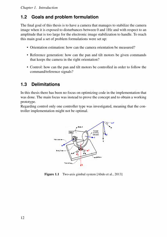
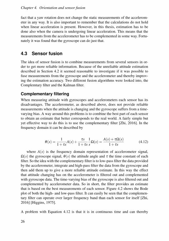
Axis Communications [Axis, 2017] is a company that today is using cameras withelectronic image stabilization. However, it can only compensate for disturbanceswith low amplitude as the electronic stabilization reduces the size of the imageshown. Due to this the stabilization could be improved by using mechanical imagestabilization as well, namely, control of the camera motors to compensate for exter-nal disturbances. In this way it would be possible to suppress larger disturbances.As mentioned above, the area of use that has been considered in this thesis is stabi-lization onboard boats, where waves and wind affect the position of the camera in amore dramatic way compared to land-based mountings. The disturbance frequencyis however smaller compared to many other environments, thereby making it espe-cially suitable for mechanical stabilization which cannot operate that fast.To measure the influence caused by disturbances, a set of sensors have been used.All the sensors were already integrated in the camera shell and software for retriev-ing data was also available.The camera construction is similar to that of a gimbal, meaning that it can movealmost freely around two orthogonal axes (pan and tilt). This kind of setup is alsooften used for handheld cameras where image stability is of importance. In Figure1.1 the construction can be seen. Pan and tilt correspond to rotations around thek-axis and e-axis, respectively.

11

Chapter 1. Introduction

1.2 Goals and problem formulation

The final goal of this thesis is to have a camera that manages to stabilize the cameraimage when it is exposed to disturbances between 0 and 1Hz and with respect to anamplitude that is too large for the electronic image stabilization to handle. To reachthis main goal a set of problem formulations were set up:

• Orientation estimation: how can the camera orientation be measured?

• Reference generation: how can the pan and tilt motors be given commandsthat keeps the camera in the right orientation?

• Control: how can the pan and tilt motors be controlled in order to follow thecommand/reference signals?

1.3 Delimitations

In this thesis there has been no focus on optimizing code in the implementation thatwas done. The main focus was instead to prove the concept and to obtain a workingprototype.Regarding control only one controller type was investigated, meaning that the con-troller implementation might not be optimal.

Figure 1.1 Two-axis gimbal system [Abdo et al., 2013]

12

1.4 Individual contributions

1.4 Individual contributions

In order to make the work of the project more efficient it was divided between theparticipants. Magnus focused on the orientation and sensor fusion, the referencegeneration and the mechanical modelling, whereas Louis focused on the systemidentification, the stepper motor modelling and the trajectory generation. The con-trol design and the hardware implementation were done together, however, Louisdid a greater part in the hardware implementation and Magnus worked more withthe control design.

1.5 Outline of the thesis

In Chapter 2 image stabilization is described in general in order to give an introduc-tion to the subject. Moreover, different techniques for stabilization are presented,including mechanical image stabilization.

Chapter 3 gives an overall view of the system that has been used. Furthermorea description of the control concept and possible disturbances are presented.

Chapter 4 describes the solution to the problem of finding camera orientation.It begins with a presentation of coordinate systems and Euler angles. It also goesinto the area of sensor fusion and in the end experimental results are presented.

Chapter 5 presents reference generation which describes how compensation sig-nals for disturbance suppression are produced. The compensation signals can alsobe seen as reference signals since the pan and tilt motors are supposed to track them.

Chapter 6 and 7 present the modelling done in the project. Three different ap-proaches are presented, namely: Physical modelling, system identification andmotion profiles.

Chapter 8 begins with a general description of control theory. Furthermore, thecontrol design for the pan and tilt motors is described and simulation results arepresented. In the end of the chapter hardware implementation for all project partsare also described.

Chapter 9 presents experimental results regarding the pan and tilt motor control.The results come from three different experiments.

In Chapter 10 a discussion and conclusion regarding the project as a whole ispresented. Moreover, possible future work is described.

13

2Image stabilization

2.1 Introduction

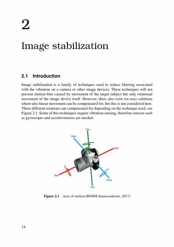
Image stabilization is a family of techniques used to reduce blurring associatedwith the vibration on a camera or other image devices. These techniques will notprevent motion blur caused by movement of the target subject but only rotationalmovement of the image device itself. However, there also exist six-axes solutionswhere also linear movement can be compensated for, but this is not considered here.Three different rotations can compensated for depending on the technique used, seeFigure 2.1. Some of this techniques require vibration sensing, therefore sensors suchas gyroscopes and accelerometers are needed.

Figure 2.1 Axes of motion [ROHM-Semiconductor, 2017]

14

2.2 Optical image stabilization

2.2 Optical image stabilization

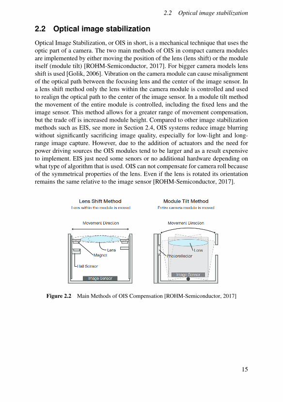
Optical Image Stabilization, or OIS in short, is a mechanical technique that uses theoptic part of a camera. The two main methods of OIS in compact camera modulesare implemented by either moving the position of the lens (lens shift) or the moduleitself (module tilt) [ROHM-Semiconductor, 2017]. For bigger camera models lensshift is used [Golik, 2006]. Vibration on the camera module can cause misalignmentof the optical path between the focusing lens and the center of the image sensor. Ina lens shift method only the lens within the camera module is controlled and usedto realign the optical path to the center of the image sensor. In a module tilt methodthe movement of the entire module is controlled, including the fixed lens and theimage sensor. This method allows for a greater range of movement compensation,but the trade off is increased module height. Compared to other image stabilizationmethods such as EIS, see more in Section 2.4, OIS systems reduce image blurringwithout significantly sacrificing image quality, especially for low-light and long-range image capture. However, due to the addition of actuators and the need forpower driving sources the OIS modules tend to be larger and as a result expensiveto implement. EIS just need some senors or no additional hardware depending onwhat type of algorithm that is used. OIS can not compensate for camera roll becauseof the symmetrical properties of the lens. Even if the lens is rotated its orientationremains the same relative to the image sensor [ROHM-Semiconductor, 2017].

Figure 2.2 Main Methods of OIS Compensation [ROHM-Semiconductor, 2017]

15

Chapter 2. Image stabilization

2.3 Sensor shift image stabilization

Sensor shift image stabilization system works by moving the camera’s sensoraround the image plane using actuators. With help of accelerometers and gyroscopesit can then sense the vibration that occurs on the camera module. The advantage withmoving the image sensor, instead of the lens as in optical image stabilization, is thatthe stabilization can be done regardless of the lens used. Another advantage is thatsome sensor shift based image stabilization implementations are capable of correct-ing camera roll rotation. A disadvantage compared to EIS is that shift modules tendto be larger and as a result more expensive to implement due to the addition ofactuators and the need for power driving sources [Golik, 2006].

2.4 Electronic image stabilization

Electronic image stabilization (EIS) is a stabilization method which uses algorithmsfor comparing contrast and pixel location between frames. The comparing is donebetween every frame and the differences are then used to create new frames whichsuffer less from vibrational motion. The fact that this stabilization method is doneby software makes it inexpensive, however, the image quality will always be re-duced. Moreover, under low light conditions or at full electronic zoom the EIS willsuffer compared to other stabilization methods [ROHM-Semiconductor, 2017].Some EIS algorithms can reduce computing time if they are provided informationabout vibrations from an accelerometer and angular velocity from a gyroscope.[Alexandre Karpenko, 2011]

2.5 Mechanic-based image stabilization

In mechanic-based image stabilization the solutions is built around the camera mod-ule. One method that is purely mechanical is "steadicam" [Golik, 2006]. Anothermethod is to build housing around the camera and compensate the vibration withthe help of actuators. To measure vibration, gyroscopes and accelerometers are usedin the same way as some of the prior technologies mentioned. Moreover, the tech-nique can compensate for bigger amplitudes of vibration than the other technolo-gies, but the drawback is the size of the housing with actuators and the need forpower driving sources, so it is not suited in small spaces.

16

3Control and systemoverview

This chapter will give an overall view of the system that has been used. Furthermorea description of the control concept and possible disturbances will be presented inthe end.

3.1 Platform

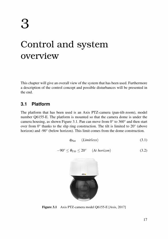
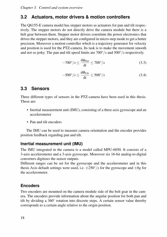
The platform that has been used is an Axis PTZ-camera (pan-tilt-zoom), modelnumber Q6155-E. The platform is mounted so that the camera dome is under thecamera housing, as shown Figure 3.1. Pan can move from 0° to 360° and then startover from 0° thanks to the slip ring construction. The tilt is limited to 20° (abovehorizon) and -90° (below horizon). This limit comes from the dome construction.

φPan (Limitless) (3.1)

−90°≤ θTilt ≤ 20° (At horizon) (3.2)

Figure 3.1 Axis PTZ-camera model Q6155-E [Axis, 2017]

17

Chapter 3. Control and system overview

3.2 Actuators, motor drivers & motion controllers

The Q6155-E camera model has stepper motors as actuators for pan and tilt respec-tively. The stepper motors do not directly drive the camera module but there is abelt gear between them. Stepper motor drivers constitute the power electronics thatdrives the stepper motors, and they are configured in micro-step mode to get a betterprecision. Moreover a motion controller which is a trajectory generator for velocityand position is used for the PTZ-camera. Its task is to make the movement smoothand not so jerky. The pan and tilt speed limits are 700°/s and 500°/s respectively.

−700°/s≤ dφPan

dt≤ 700°/s (3.3)

−500°/s≤ dθTilt

dt≤ 500°/s (3.4)

3.3 Sensors

Three different types of sensors in the PTZ-camera have been used in this thesis.These are:

• Inertial measurement unit (IMU), consisting of a three-axis gyroscope and anaccelerometer

• Pan and tilt encoders

The IMU can be used to measure camera orientation and the encoder providesposition feedback regarding pan and tilt.

Inertial measurement unit (IMU)The IMU integrated in the camera is a model called MPU-6050. It consists of a3-axis accelerometer and a 3-axis gyroscope. Moreover six 16-bit analog-to-digitalconverters digitizes the sensor outputs.Different ranges can be set for the gyroscope and the accelerometer and in thisthesis Axis default settings were used, i.e. ±250/s for the gyroscope and ±8g forthe accelerometer.

EncodersTwo encoders are mounted on the camera module side of the belt gear in the cam-era. The encoders provide information about the angular position for both pan andtilt by dividing a 360 rotation into discrete steps. A certain sensor value therebycorresponds to a certain angle relative to the origin position.

18

3.4 System architecture

3.4 System architecture

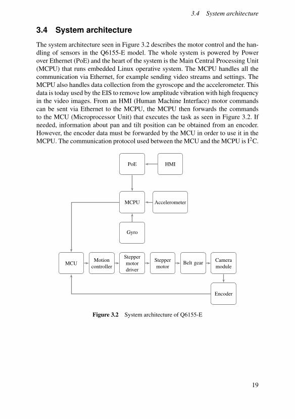
The system architecture seen in Figure 3.2 describes the motor control and the han-dling of sensors in the Q6155-E model. The whole system is powered by Powerover Ethernet (PoE) and the heart of the system is the Main Central Processing Unit(MCPU) that runs embedded Linux operative system. The MCPU handles all thecommunication via Ethernet, for example sending video streams and settings. TheMCPU also handles data collection from the gyroscope and the accelerometer. Thisdata is today used by the EIS to remove low amplitude vibration with high frequencyin the video images. From an HMI (Human Machine Interface) motor commandscan be sent via Ethernet to the MCPU, the MCPU then forwards the commandsto the MCU (Microprocessor Unit) that executes the task as seen in Figure 3.2. Ifneeded, information about pan and tilt position can be obtained from an encoder.However, the encoder data must be forwarded by the MCU in order to use it in theMCPU. The communication protocol used between the MCU and the MCPU is I2C.

Cameramodule

Belt gearSteppermotor

Steppermotordriver

MotioncontrollerMCU

Encoder

Gyro

MCPU Accelerometer

PoE HMI

Figure 3.2 System architecture of Q6155-E

19

Chapter 3. Control and system overview

3.5 Control concept

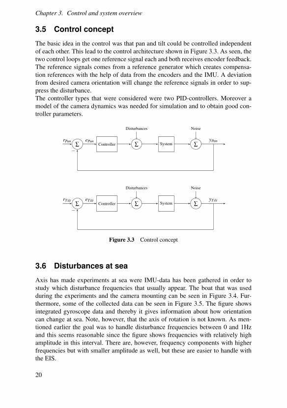
The basic idea in the control was that pan and tilt could be controlled independentof each other. This lead to the control architecture shown in Figure 3.3. As seen, thetwo control loops get one reference signal each and both receives encoder feedback.The reference signals comes from a reference generator which creates compensa-tion references with the help of data from the encoders and the IMU. A deviationfrom desired camera orientation will change the reference signals in order to sup-press the disturbance.The controller types that were considered were two PID-controllers. Moreover amodel of the camera dynamics was needed for simulation and to obtain good con-troller parameters.

∑ Controller ∑

Disturbances

System ∑

Noise

∑

Disturbances

Controller∑ System ∑

Noise

rPan ePan yPan

−

rTilt eTilt yTilt

−

Figure 3.3 Control concept

3.6 Disturbances at sea

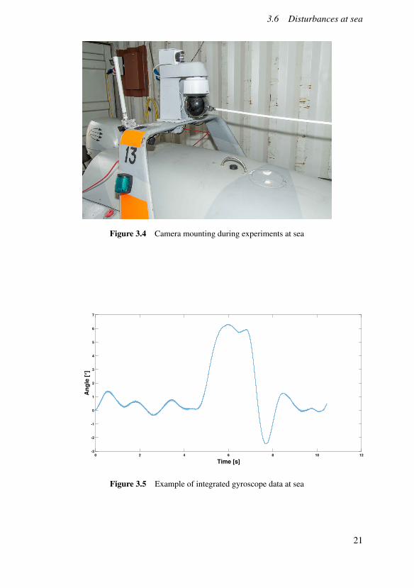
Axis has made experiments at sea were IMU-data has been gathered in order tostudy which disturbance frequencies that usually appear. The boat that was usedduring the experiments and the camera mounting can be seen in Figure 3.4. Fur-thermore, some of the collected data can be seen in Figure 3.5. The figure showsintegrated gyroscope data and thereby it gives information about how orientationcan change at sea. Note, however, that the axis of rotation is not known. As men-tioned earlier the goal was to handle disturbance frequencies between 0 and 1Hzand this seems reasonable since the figure shows frequencies with relatively highamplitude in this interval. There are, however, frequency components with higherfrequencies but with smaller amplitude as well, but these are easier to handle withthe EIS.

20

3.6 Disturbances at sea

Figure 3.4 Camera mounting during experiments at sea

0 2 4 6 8 10 12

Time [s]

-3

-2

-1

0

1

2

3

4

5

6

7

An

gle

[°]

Figure 3.5 Example of integrated gyroscope data at sea

21

4Orientation and sensorfusion

The first problem that had to be solved in the thesis was how to obtain the cameraorientation from the IMU. This problem lead into the area of sensor fusion and twodifferent methods for estimating orientation, the Kalman and Complementary filter.The performance of them both was tested and compared in order to implement thebest one.This chapter will describe the whole process of orientation estimation, starting outby introducing necessary coordinate systems and ending with the presentation ofreal orientation data.

4.1 Coordinate systems

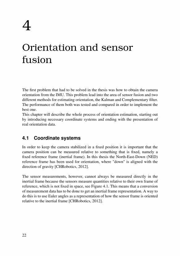
In order to keep the camera stabilized in a fixed position it is important that thecamera position can be measured relative to something that is fixed, namely afixed reference frame (inertial frame). In this thesis the North-East-Down (NED)reference frame has been used for orientation, where "down" is aligned with thedirection of gravity [CHRobotics, 2012].

The sensor measurements, however, cannot always be measured directly in theinertial frame because the sensors measure quantities relative to their own frame ofreference, which is not fixed in space, see Figure 4.1. This means that a conversionof measurement data has to be done to get an inertial frame representation. A way todo this is to use Euler angles as a representation of how the sensor frame is orientedrelative to the inertial frame [CHRobotics, 2012].

22

4.1 Coordinate systems

Figure 4.1 Inertial reference frame relative to unfixed sensor frame [Alves Netoet al., 2009]

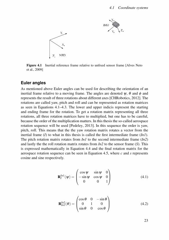
Euler anglesAs mentioned above Euler angles can be used for describing the orientation of aninertial frame relative to a moving frame. The angles are denoted ψ , θ and φ andrepresents the result of three rotations about different axes [CHRobotics, 2012]. Therotations are called yaw, pitch and roll and can be represented as rotation matricesas seen in Equations 4.1–4.3. The lower and upper indicis represent the startingand ending frame for the rotation. To get a rotation matrix representing all threerotations, all three rotation matrices have to multiplied, but one has to be careful,because the order of the multiplication matters. In this thesis the so-called aerospacerotation sequence will be used [Pedeley, 2013]. In this sequence the order is yaw,pitch, roll. This means that the the yaw rotation matrix rotates a vector from theinertial frame (I) to what in this thesis is called the first intermediate frame (In1).The pitch rotation matrix rotates from In1 to the second intermediate frame (In2)and lastly the the roll rotation matrix rotates from In2 to the sensor frame (S). Thisis expressed mathematically in Equation 4.4 and the final rotation matrix for theaerospace rotation sequence can be seen in Equation 4.5, where c and s representscosine and sine respectively.

RIn1I (ψ) =

cosψ sinψ 0−sinψ cosψ 0

0 0 1

(4.1)

RIn2In1(θ) =

cosθ 0 −sinθ

0 1 0sinθ 0 cosθ

(4.2)

23

Chapter 4. Orientation and sensor fusion

RSIn2(φ) =

1 0 00 cosφ sinφ

0 −sinφ cosφ

(4.3)

RSI (φ ,θ ,ψ) = RS

In2(φ)RIn2In1(θ)R

In1I (ψ) (4.4)

RSI (φ ,θ ,ψ) =

c(θ)c(ψ) c(θ)s(ψ) −s(θ)c(ψ)s(θ)s(φ)− c(φ)s(ψ) c(φ)c(ψ)+ s(θ)s(φ)s(ψ) c(θ)s(φ)c(φ)c(ψ)s(θ)+ s(φ)s(ψ) c(φ)s(θ)s(ψ)− c(ψ)s(φ) c(θ)c(φ)

(4.5)

Equation 4.5 can be used for estimating the pitch and roll angles from ac-celerometer readings which is described in Section 4.2 [Pedeley, 2013]. Gyro read-ings however, cannot be represented in the inertial frame using 4.5. For this therotation matrix in Equation 4.6 is needed. The axes of the IMU-sensor frame in thisthesis are denoted Xs, Ys and Zs and when the camera is horizontal Xs is in the oppo-site direction of gravity. Zs is in the optical axis direction and Ys is perpendicular tothem both. So if the angular velocities in the sensor frame are denoted xvel , yvel andzvel the Euler angle rates can be calculated as in Equation 4.7 [CHRobotics, 2012].

D(φ ,θ ,ψ) =

1 sinφ tanθ cosφ tanθ

0 cosφ −sinφ

0 sinφ/cosθ cosφ/cosθ

(4.6)

φ

θ

ψ

=

1 sinφ tanθ cosφ tanθ

0 cosφ −sinφ

0 sinφ/cosθ cosφ/cosθ

zvel

yvelxvel

(4.7)

An important thing to notice about Equation 4.7 is that a pitch angle θ of 90

will cause some matrix elements to diverge towards infinity. This is a phenomenoncalled gimbal lock which sets a limitation for Euler angles. This leads to the con-clusion that Euler angles should not be used in applications where the pitch anglewill get near ±90 [CHRobotics, 2012].

24

4.2 Attitude estimation with accelerometers

4.2 Attitude estimation with accelerometers

Accelerometers can be used for both sensing linear acceleration and strength ofthe gravitational field. The latter can be used for estimating attitude relative to theground, but only under static conditions, i.e. no linear acceleration. To do this Equa-tion 4.5 can used as it describes the relationship between the inertial and sensorframe vector representation [Pedeley, 2013]. Under static conditions the relationlooks as follows:

ZsYsXs

= RSI (φ ,θ ,ψ)

00−1

(4.8)

where -1 represents -1g. The minus sign is necessary in order to get alignmentbetween the sensor frame and inertial frame when all Euler angles are zero, i.e. norotation has been done. However, this only holds when the camera is mounted withthe chassi upwards, see Figure 3.1. In the opposite case the -1g needs to be replacedwith just 1g. This is however not how the camera is supposed to be mounted. More-over, the vector elements in the sensor frame are also represented in the unit g. Ifthe multiplication in Equation 4.8 is carried out the following is obtained:

ZsYsXs

=

sin(θ)−cos(θ)sin(φ)−cos(θ)cos(φ)

(4.9)

Solving for θ and φ gives:

φ = atan2

(−Ys,−Xs

)(4.10)

θ = atan2

(Zs,√

Y 2s +X2

s

)(4.11)

where atan2(y,x) returns the arcus tangent of y/x with respect to sign of theinput parameters. Thereby the right quadrant is determined [Bilting and Skansholm,2011].

The calculations above show that only the pitch and roll angles can be estimatedusing an accelerometer and the aerospace rotation sequence. This comes from the

25

Chapter 4. Orientation and sensor fusion

fact that a yaw rotation does not change the static measurements of the accelerom-eter in any way. It is also important to remember that the calculations do not holdwhen linear acceleration is present. However, in this thesis, estimation has to bedone also when the camera is undergoing linear acceleration. This means that themeasurements from the accelerometer has to be complemented in some way. Fortu-nately it was found that the gyroscope can do just that.

4.3 Sensor fusion

The idea of sensor fusion is to combine measurements from several sensors in or-der to get more reliable information. Because of the unreliable attitude estimationdescribed in Section 4.2 it seemed reasonable to investigate if it was possible tofuse measurements from the gyroscope and the accelerometer and thereby improv-ing the estimation accuracy. Two different fusion algorithms were looked into, theComplemtary filter and the Kalman filter.

Complementary filteringWhen measuring attitude with gyroscopes and accelerometers each sensor has itsdisadvantages. The accelerometer, as described above, does not provide reliablemeasurements when the attitude is changing and the gyroscope suffers from a time-varying bias. A way around this problems is to combine the best part of each sensorto obtain an estimate that better corresponds to the real world. A fairly simple butyet effective way to do this is to use the complementary filter [Zhi, 2016]. In thefrequency domain it can be described by

θ(s) =1

1+ τsA(s)+

τs1+ τs

1s

Ω(s) =A(s)+ τΩ(s)

1+ τs(4.12)

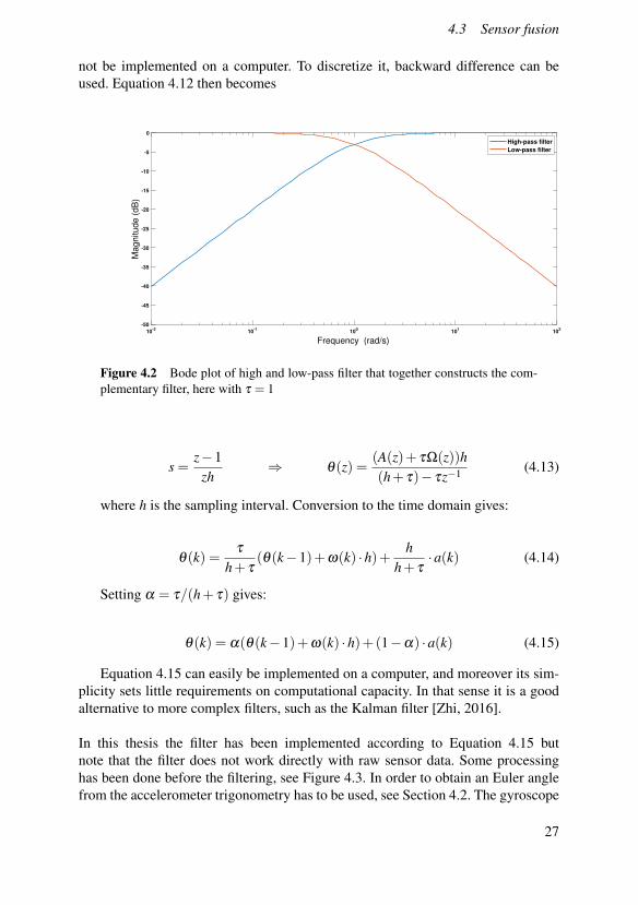
where A(s) is the frequency domain representation of accelerometer signal,Ω(s) the gyroscope signal, θ(s) the attitude angle and τ the time constant of eachfilter. So the idea with the complementary filter is to low-pass filter the data providedby the accelerometer, integrate and high-pass filter the data from the gyroscope andthen add them up to give a more reliable attitude estimate. In this way the effectthat attitude changing has on the accelerometer is filtered out and complementedwith gyroscope data. The time-varying bias of the gyroscope is also filtered out andcomplemented by accelerometer data. So in short, the filter provides an estimatethat is based on the best measurements of each sensor. Figure 4.2 shows the Bodeplot of both the high- and low-pass filter. It can easily be seen that the complemen-tary filter can operate over larger frequency band than each sensor for itself [Zhi,2016] [Higgins, 1975].

A problem with Equation 4.12 is that it is in continuous time and can thereby

26

4.3 Sensor fusion

not be implemented on a computer. To discretize it, backward difference can beused. Equation 4.12 then becomes

10-2

10-1

100

101

102

-50

-45

-40

-35

-30

-25

-20

-15

-10

-5

0M

agnitude (

dB

)High-pass filter

Low-pass filter

Frequency (rad/s)

Figure 4.2 Bode plot of high and low-pass filter that together constructs the com-plementary filter, here with τ = 1

s =z−1

zh⇒ θ(z) =

(A(z)+ τΩ(z))h(h+ τ)− τz−1 (4.13)

where h is the sampling interval. Conversion to the time domain gives:

θ(k) =τ

h+ τ(θ(k−1)+ω(k) ·h)+ h

h+ τ·a(k) (4.14)

Setting α = τ/(h+ τ) gives:

θ(k) = α(θ(k−1)+ω(k) ·h)+(1−α) ·a(k) (4.15)

Equation 4.15 can easily be implemented on a computer, and moreover its sim-plicity sets little requirements on computational capacity. In that sense it is a goodalternative to more complex filters, such as the Kalman filter [Zhi, 2016].

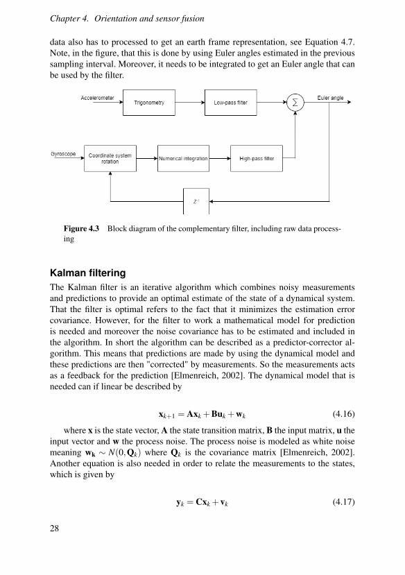
In this thesis the filter has been implemented according to Equation 4.15 butnote that the filter does not work directly with raw sensor data. Some processinghas been done before the filtering, see Figure 4.3. In order to obtain an Euler anglefrom the accelerometer trigonometry has to be used, see Section 4.2. The gyroscope

27

Chapter 4. Orientation and sensor fusion

data also has to processed to get an earth frame representation, see Equation 4.7.Note, in the figure, that this is done by using Euler angles estimated in the previoussampling interval. Moreover, it needs to be integrated to get an Euler angle that canbe used by the filter.

Figure 4.3 Block diagram of the complementary filter, including raw data process-ing

Kalman filteringThe Kalman filter is an iterative algorithm which combines noisy measurementsand predictions to provide an optimal estimate of the state of a dynamical system.That the filter is optimal refers to the fact that it minimizes the estimation errorcovariance. However, for the filter to work a mathematical model for predictionis needed and moreover the noise covariance has to be estimated and included inthe algorithm. In short the algorithm can be described as a predictor-corrector al-gorithm. This means that predictions are made by using the dynamical model andthese predictions are then "corrected" by measurements. So the measurements actsas a feedback for the prediction [Elmenreich, 2002]. The dynamical model that isneeded can if linear be described by

xk+1 = Axk +Buk +wk (4.16)

where x is the state vector, A the state transition matrix, B the input matrix, u theinput vector and w the process noise. The process noise is modeled as white noisemeaning wk ∼ N(0,Qk) where Qk is the covariance matrix [Elmenreich, 2002].Another equation is also needed in order to relate the measurements to the states,which is given by

yk = Cxk +vk (4.17)

28

4.3 Sensor fusion

where C is the observation matrix, y the sensor measurements and vk themeasurement noise. The measurement noise can also be described as white noisevk ∼ N(0,Rk) with covariance matrix Rk. With the equations above the predictionpart of the algorithm can be described as follows:

xk+1 = Axk +Buk (4.18)

Pk+1 = APkAT +Qk (4.19)

where Equation 4.18 predicts the future state vector xk+1 and the second, Equa-tion 4.19, predicts the estimation error covariance of the state. The next step of thealgorithm is the update, where the predictions are corrected by measurements. Thisis done in the following way:

Kk+1 = Pk+1CT (CPk+1CT +Rk+1)−1 (4.20)

xk+1 = xk+1 +Kk+1(yk+1−Cxk+1) (4.21)Pk+1 = (I−Kk+1C)Pk+1 (4.22)

where K is known as the Kalman gain. This gain is what minimizes the stateestimation error when converged to a stationary value [Glad and Ljung, 2003].Equations 4.18–4.22 contain all steps of the algorithm and after 4.22 it is repeated.This iterative behavior and the fact that every iteration takes approximately the sametime makes the algorithm well-suited for real-time applications [Elmenreich, 2002].

In order to predict the pitch and roll angle, using the gyroscope and Equation4.7 only, the following dynamical model was considered:

θk = θk−1 +(θk−bk−1)h (4.23)

where θ represents the pitch angle, θ the pitch rate, b the bias of the pitch rateand h the sampling interval of the IMU [Sloth Lauszus, 2012]. The same model canbe applied to predict the roll and yaw angle.In order to get a state space representation like the one presented in Equation 4.16the following state vector can be chosen:

x =

(θ

b

)(4.24)

leading to the state space representation

29

Chapter 4. Orientation and sensor fusion

(θkbk

)=

(1 −h0 1

)(θk−1bk−1

)+

(h0

)θk +wk (4.25)

where the noise is assumed to be uncorrelated meaning that the covariance ma-trix Qk looks as follows

Qk =

(Qθ 00 Qb

)(4.26)

where Qθ and Qb represents the variance of the noise that is corrupting theestimation of θ and b respectively. In this case the noise in θ comes from the gy-roscope measurements [Pycke, 2006]. Due to this fact that variance could be foundby experiment.

In the update step of the algorithm the accelerometer can be used to correct themeasurements made by the gyroscope [Sloth Lauszus, 2012]. This is done by usingthe accelerometer as described in Section 4.2. The relation between the measure-ments and the the states according to Equation 4.17 is then given by

yk =(

1 0)(

θkb

)+ vk (4.27)

where v is a scalar meaning that the measurement noise covariance matrix Rk isjust the variance of the measurement noise, i.e. the accelerometer noise. This valuecould also be found experimentally.

Note that only the roll and pitch angles could be estimated with the Kalman filter.Although the yaw angle could be predicted it could never be corrected by the ac-celerometer. The same holds for the Complementary filter. This was a problem thathad to be solved in order to get the reference generator working.To clarify it can also be mentioned that one Complementary/Kalman filter eitherestimates roll or pitch. To obtain both, two filters are needed.

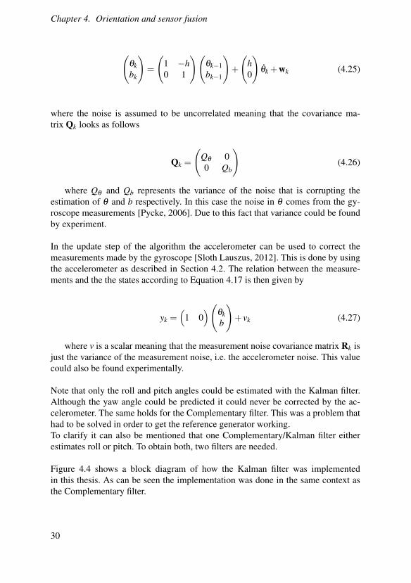
Figure 4.4 shows a block diagram of how the Kalman filter was implementedin this thesis. As can be seen the implementation was done in the same context asthe Complementary filter.

30

4.4 Result and discussion

Figure 4.4 Block diagram of the Kalman filter, including raw data processing

4.4 Result and discussion

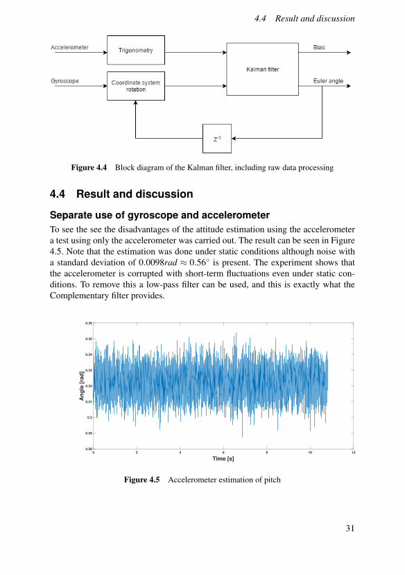
Separate use of gyroscope and accelerometerTo see the see the disadvantages of the attitude estimation using the accelerometera test using only the accelerometer was carried out. The result can be seen in Figure4.5. Note that the estimation was done under static conditions although noise witha standard deviation of 0.0098rad ≈ 0.56 is present. The experiment shows thatthe accelerometer is corrupted with short-term fluctuations even under static con-ditions. To remove this a low-pass filter can be used, and this is exactly what theComplementary filter provides.

0 2 4 6 8 10 12

Time [s]

0.28

0.29

0.3

0.31

0.32

0.33

0.34

0.35

0.36

An

gle

[ra

d]

Figure 4.5 Accelerometer estimation of pitch

31

Chapter 4. Orientation and sensor fusion

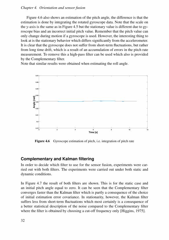
Figure 4.6 also shows an estimation of the pitch angle, the difference is that theestimation is done by integrating the rotated gyroscope data. Note that the scale onthe y-axis is the same as in Figure 4.5 but the stationary value is different due to gy-roscope bias and an incorrect initial pitch value. Remember that the pitch value canonly change during motion if a gyroscope is used. However, the interesting thing tolook at is the stationary behavior which differs significantly from the accelerometer.It is clear that the gyroscope does not suffer from short-term fluctuations, but ratherfrom long time drift, which is a result of an accumulation of errors in the pitch ratemeasurement. To remove this a high-pass filter can be used which also is providedby the Complementary filter.Note that similar results were obtained when estimating the roll angle.

0 2 4 6 8 10 12

Time [s]

0.19

0.2

0.21

0.22

0.23

0.24

0.25

0.26

0.27

An

gle

[ra

d]

Figure 4.6 Gyroscope estimation of pitch, i.e. integration of pitch rate

Complementary and Kalman filteringIn order to decide which filter to use for the sensor fusion, experiments were car-ried out with both filters. The experiments were carried out under both static anddynamic conditions.

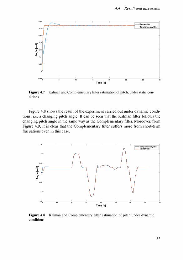
In Figure 4.7 the result of both filters are shown. This is for the static case andan initial pitch angle equal to zero. It can be seen that the Complementary filterconverges faster than the Kalman filter which is partly a consequence of the choiceof initial estimation error covariance. In stationarity, however, the Kalman filtersuffers less from short-term fluctuations which most certainly is a consequence ofa better statistical description of the noise compared to the Complementary filterwhere the filter is obtained by choosing a cut-off frequency only [Higgins, 1975].

32

4.4 Result and discussion

0 5 10 15 20 25 30 35

Time [s]

-0.05

0

0.05

0.1

0.15

0.2

0.25

0.3

0.35

An

gle

[ra

d]

Kalman filter

Complementary filter

Figure 4.7 Kalman and Complementary filter estimation of pitch, under static con-ditions

Figure 4.8 shows the result of the experiment carried out under dynamic condi-tions, i.e. a changing pitch angle. It can be seen that the Kalman filter follows thechanging pitch angle in the same way as the Complementary filter. Moreover, fromFigure 4.9, it is clear that the Complementary filter suffers more from short-termflucuations even in this case.

0 10 20 30 40 50 60 70 80

Time [s]

-1.5

-1

-0.5

0

0.5

1

1.5

An

gle

[ra

d]

Complementary filterKalman filter

Figure 4.8 Kalman and Complementary filter estimation of pitch under dynamicconditions

33

Chapter 4. Orientation and sensor fusion

38 40 42 44 46 48

Time [s]

0.15

0.2

0.25

0.3

0.35

0.4

0.45

An

gle

[ra

d]

Kalman filter

Complementary filter

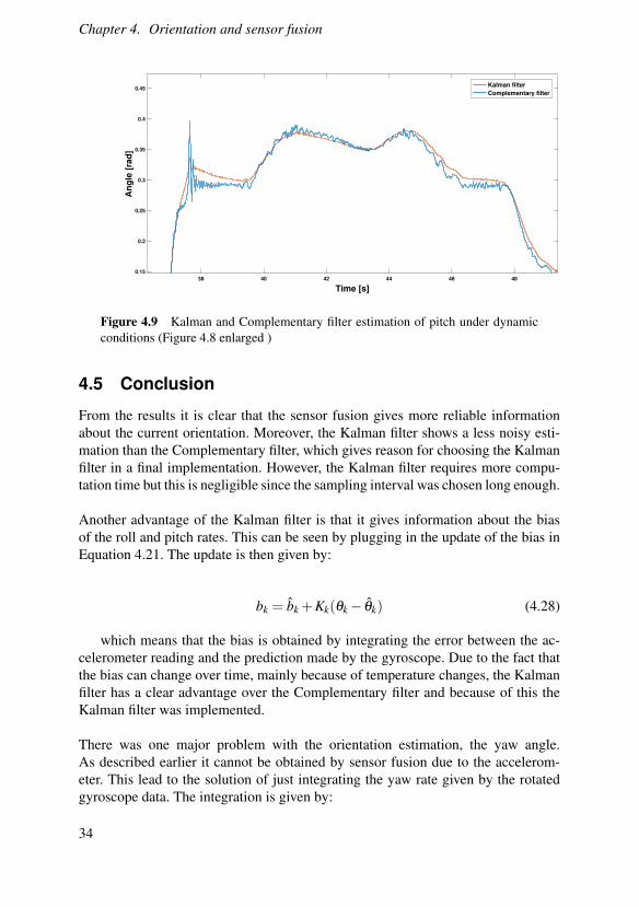
Figure 4.9 Kalman and Complementary filter estimation of pitch under dynamicconditions (Figure 4.8 enlarged )

4.5 Conclusion

From the results it is clear that the sensor fusion gives more reliable informationabout the current orientation. Moreover, the Kalman filter shows a less noisy esti-mation than the Complementary filter, which gives reason for choosing the Kalmanfilter in a final implementation. However, the Kalman filter requires more compu-tation time but this is negligible since the sampling interval was chosen long enough.

Another advantage of the Kalman filter is that it gives information about the biasof the roll and pitch rates. This can be seen by plugging in the update of the bias inEquation 4.21. The update is then given by:

bk = bk +Kk(θk− θk) (4.28)

which means that the bias is obtained by integrating the error between the ac-celerometer reading and the prediction made by the gyroscope. Due to the fact thatthe bias can change over time, mainly because of temperature changes, the Kalmanfilter has a clear advantage over the Complementary filter and because of this theKalman filter was implemented.

There was one major problem with the orientation estimation, the yaw angle.As described earlier it cannot be obtained by sensor fusion due to the accelerom-eter. This lead to the solution of just integrating the yaw rate given by the rotatedgyroscope data. The integration is given by:

34

4.5 Conclusion

ψ =∫ t

t0

dψ

dτdτ (4.29)

This means that the yaw angle always will be given the value zero initially,regardless of true orientation relative to the north-east direction. Another issue isthe bias which will not be estimated continuously. To solve this a yaw rate biasestimation was implemented to be carried out under static conditions. The idea ofthe estimation was to gather as much yaw rate data as possible under a certain timeand then take the mean value of it in order to obtain a bias estimate. This gavea decent result, meaning that the drift was reasonable. However, under changingtemperatures it might be worse.The only way to solve the problem regarding true orientation is to provide additionaldata to the camera, from a magnetometer for example. This data can then be fusedwith the gyroscope in order to get a more reliable estimate. However, the integrationwas enough to prove the concept of the thesis.

35

5Reference generation

The estimation of the camera orientation opened up for the opportunity to createa feedback path for the upcoming control design. This was the initial thought, butthis was later reconsidered since the camera actuators do not control pitch and yawdirectly, unless the camera chassi is horizontal. The actuators do rather control panand tilt which is the camera orientation relative its own chassi and not the NED-frame. This fact lead to the idea of reference generation, which means that referencesignals for pan and tilt would be created in order to reach the desired NED-frameorientation. To do this two new frames had to be introduced resulting in a total offour frames, described as follows:

• NED-frame - North-East-Down inertial frame

• Sensor frame - frame which follows the movements of the sensor.

• Desired frame - frame which is oriented in the desired camera orientationrelative to the NED-frame.

• Chassi frame - frame which follows the movements of the camera chassi andis thereby an inertial frame for pan and tilt motions.

With the frames defined the problem could be stated as follows: How does thesensor frame need to be oriented relative to the Chassi frame in order to align withthe desired frame?

The first step of the solution requires a rotation matrix which describes the ro-tation that has to be done relative to the Chassi frame. This can be expressed asfollows:

RDesiredChassi = RDesired

NED RNEDSensorR

SensorChassi (5.1)

where the matrices on the left have the same look as in Equation 4.5 and itsinverse, which means that three sets of Euler angles have to be known in order to

36

5.1 Extracting Euler angles from a rotation matrix

get a matrix containing only numerical values. The angles that create the matricesare the following:

• RDesiredNED - matrix defined by the desired Euler angles relative to the NED-

frame (φd ,θd ,ψd), which is given by the user.

• RNEDSensor - matrix defined by the current Euler angles of the sensor frame rela-

tive to the NED-frame (φ ,θ ,ψ), i.e. the angles estimated with IMU-data.

• RSensorChassi - matrix defined by the current Euler angles of the sensor frame rela-

tive to the Chassi frame (φc,θc,ψc), where ψc and θc is given by the pan andtilt encoders. φc is always equal to zero since a roll rotation cannot be donerelative to the Chassi frame.

This means that RDesiredChassi can be created at any time. Furthermore, if it is possible

to find Euler angles relative to the Chassi frame that directly creates RDesiredChassi these

can be used as references for pan and tilt. Obviously, Euler angle extraction is thenneeded.

5.1 Extracting Euler angles from a rotation matrix

The extraction of Euler angles can be done by first expressing RDesiredChassi as an arbi-

trary rotation matrix given by

RDesiredChassi =

R00 R01 R02R10 R11 R12R20 R21 R22

(5.2)

and then match the matrix elements in Equation 4.5 with it [Day, 2012]. Theroll angle can be extracted in the following way:

φc = atan2(R12,R22) = atan2(s(φc)c(θc),c(φc)c(θc)) (5.3)

Moreover the pitch angle can be extracted by first computing:

cos(θc) =√

R200 +R2

01 (5.4)

and then

θc = atan2(−R02,c(θc)) (5.5)

37

Chapter 5. Reference generation

Lastly ψc can be obtained by inserting the pitch and roll angles into Equation4.5 with ψc = 0. The transpose of the resulting matrix can then be multiplied withRDesired

Chassi to get a result which can be matched with Equation 4.1. The matchingresults in:

ψc = atan2(s(φc)R20− c(φc)R10,c(φc)R11− s(φc)R21) (5.6)

which completes the Euler angle extraction [Day, 2012].

The calculations made make it possible to use ψc as a reference for pan and θcas a reference for tilt since those values will result in an alignment of the sensorframe and the desired frame. Note, however, that the angle φc cannot be used asa reference in this thesis due to the fact that the camera cannot do a roll rotationrelative to the chassi frame. This means that the desired orientation relative to theNED-frame is not possible to reach in all cases.

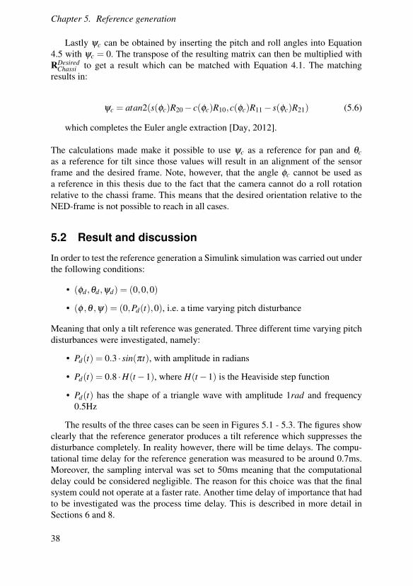
5.2 Result and discussion

In order to test the reference generation a Simulink simulation was carried out underthe following conditions:

• (φd ,θd ,ψd) = (0,0,0)

• (φ ,θ ,ψ) = (0,Pd(t),0), i.e. a time varying pitch disturbance

Meaning that only a tilt reference was generated. Three different time varying pitchdisturbances were investigated, namely:

• Pd(t) = 0.3 · sin(πt), with amplitude in radians

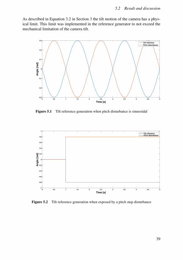
• Pd(t) = 0.8 ·H(t−1), where H(t−1) is the Heaviside step function

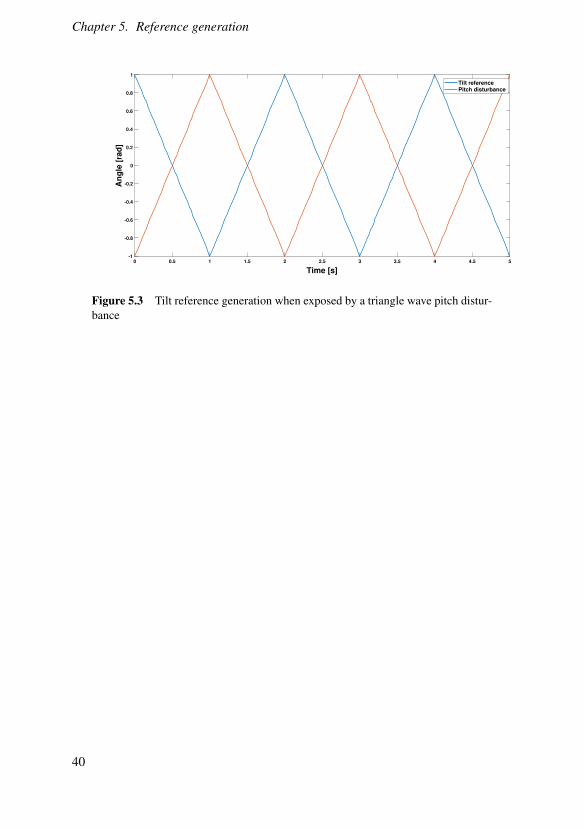
• Pd(t) has the shape of a triangle wave with amplitude 1rad and frequency0.5Hz

The results of the three cases can be seen in Figures 5.1 - 5.3. The figures showclearly that the reference generator produces a tilt reference which suppresses thedisturbance completely. In reality however, there will be time delays. The compu-tational time delay for the reference generation was measured to be around 0.7ms.Moreover, the sampling interval was set to 50ms meaning that the computationaldelay could be considered negligible. The reason for this choice was that the finalsystem could not operate at a faster rate. Another time delay of importance that hadto be investigated was the process time delay. This is described in more detail inSections 6 and 8.

38

5.2 Result and discussion

As described in Equation 3.2 in Section 3 the tilt motion of the camera has a phys-ical limit. This limit was implemented in the reference generator to not exceed themechanical limitation of the camera tilt.

0 0.5 1 1.5 2 2.5 3 3.5 4 4.5 5

Time [s]

-0.3

-0.2

-0.1

0

0.1

0.2

0.3

An

gle

[ra

d]

Tilt reference

Pitch disturbance

Figure 5.1 Tilt reference generation when pitch disturbance is sinusoidal

0 0.5 1 1.5 2 2.5 3 3.5 4 4.5 5

Time [s]

-1

-0.8

-0.6

-0.4

-0.2

0

0.2

0.4

0.6

0.8

1

An

gle

[ra

d]

Tilt referencePitch disturbance

Figure 5.2 Tilt reference generation when exposed by a pitch step disturbance

39

Chapter 5. Reference generation

0 0.5 1 1.5 2 2.5 3 3.5 4 4.5 5

Time [s]

-1

-0.8

-0.6

-0.4

-0.2

0

0.2

0.4

0.6

0.8

1

An

gle

[ra

d]

Tilt referencePitch disturbance

Figure 5.3 Tilt reference generation when exposed by a triangle wave pitch distur-bance

40

6Modelling

A model of the camera was needed for simulation and for finding appropriate con-trol parameters for the controller. In this thesis this was done in three ways. Thefirst approach was to model the camera with a psychical model, i.e., with the lawsof nature. However, this was never used in the control design due to the extensivework of finding the right physical parameters and also due to the fact that it wasactually the motion controllers that decided the behavior of camera movements.This realization lead to the idea of modelling the camera with motion profiles, whichis what is used by the motion controller. This approach was however not used in thefinal control design, due to lack of time. The idea will be presented in Chapter 7though.The third approach was to model the system with system identification. This wasdone successfully and was later used in the control design.In the sections below the physical modelling and the system identification is de-scribed. The motion profile is as mentioned described in Chapter 7.Even though the physical model and the motion profile was not used to reach thefinal result of the thesis they are most relevant to describe since this can be used inlater projects which might go deeper into this.

41

Chapter 6. Modelling

6.1 Physical modelling

The Axis camera uses stepper motors for driving both pan and tilt. However, thestepper motors do not drive the mechanical system directly. In between there arebelt gears. Due to this the physical modelling was divided into three parts as seen inFigure 6.1. For the mechanical system block a two-axis gimbal model was investi-gated. In the three upcoming subsections mathematical models for each subsystemwill be presented.

Actuators Gears Mechanical dynamics

Figure 6.1 Physical model of the system

Stepper motorsThe Axis camera model uses stepper motors as actuators for moving pan and tilt.The are three main types of stepper motors:

• Permanent magnet stepper motors

• Hybrid stepper motors

• Variable reluctance steppers motor

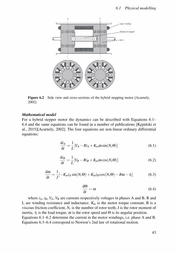
The Axis camera uses hybrid stepper motors and as the name applies it is a com-bination of a permanent magnet and a variable reluctance stepper motor. In Figure6.2 it can be seen that the windings create the stator poles and that a permanentmagnet is mounted on the rotor. Each pole has between two and six teeth and mostcommonly there are eight stator poles. The windings are two in total and each wind-ing is placed on four of the eight stator poles: winding A is placed on poles 1, 3, 5,7 and winding B is placed on poles 2, 4, 6, 8. Successive poles of each winding arewound in the opposite sense.The rotor is a cylindrical permanent magnet, magnetized along the axis with radialsoft iron teeth.The main principle of the motor is that when certain poles generate magnetic flux,the rotor will move until the airgap reluctance of the flux path is minimized [Acar-nely, 2002].

42

6.1 Physical modelling

Figure 6.2 Side view and cross-sections of the hybrid stepping motor [Acarnely,2002]

Mathematical modelFor a hybrid stepper motor the dynamics can be described with Equations 6.1–6.4 and the same equations can be found in a number of publications [Kepinski etal., 2015][Acarnely, 2002]. The four equations are non-linear ordinary differentialequations:

diAdt

=1L[VA−RiA +Kmω sin(NrΘ)] (6.1)

diBdt

=1L[VB−RiB +Kmω cos(NrΘ)] (6.2)

dω

dt=

1J[−KmiA sin(NrΘ)+KmiB cos(NrΘ)−Bω− τl ] (6.3)

dΘ

dt= ω (6.4)

where iA, iB, VA, VB are currents respectively voltages in phases A and B. R andL are winding resistance and inductance. Km is the motor torque constant, B is aviscous friction coefficient, Nr is the number of rotor teeth, J is the rotor moment ofinertia, τl is the load torque, ω is the rotor speed and Θ is its angular position.Equations 6.1–6.2 determine the current in the motor windings, i.e. phase A and B.Equations 6.3–6.4 correspond to Newton’s 2nd law of rotational motion.

43

Chapter 6. Modelling

Belt GearA belt gear is placed between the stepper motors and the two-axis gimbal and doesthereby add more dynamics to the system. To transform angular velocity (ωn) andtorque (Mn) from the stepper motor side to the gimbal side the following equationscan be used:

M1 =±rM2 (6.5)

ω2 =∓rω1 (6.6)

Where r is ratio of circumference between the belt wheels, M1 the torque of wheel1 and ω1 the angular velocity of wheel 1. The same notation is used for wheel 2 butwith the index 2 instead [Ljung, 2007].

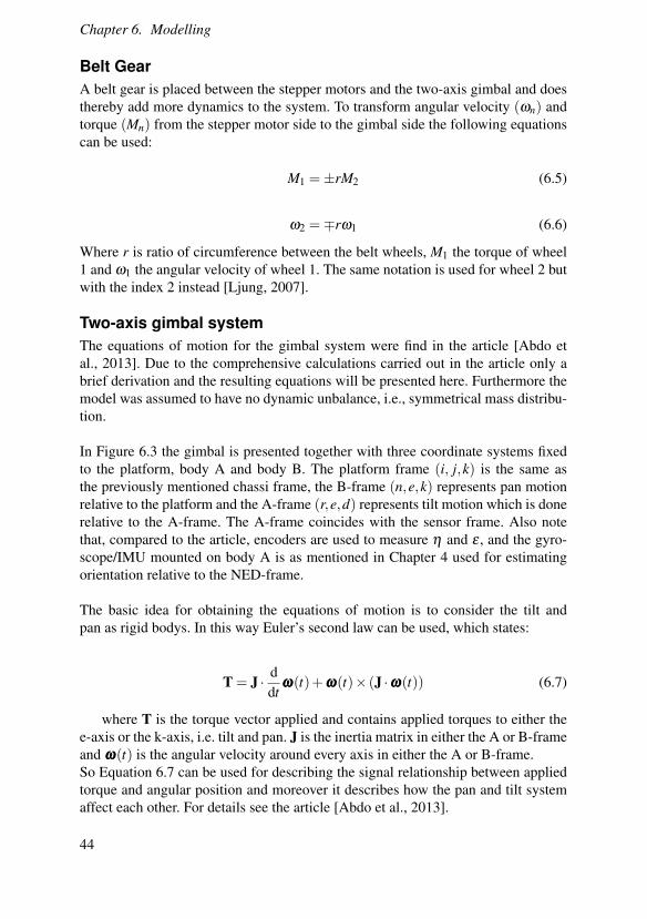
Two-axis gimbal systemThe equations of motion for the gimbal system were find in the article [Abdo etal., 2013]. Due to the comprehensive calculations carried out in the article only abrief derivation and the resulting equations will be presented here. Furthermore themodel was assumed to have no dynamic unbalance, i.e., symmetrical mass distribu-tion.

In Figure 6.3 the gimbal is presented together with three coordinate systems fixedto the platform, body A and body B. The platform frame (i, j,k) is the same asthe previously mentioned chassi frame, the B-frame (n,e,k) represents pan motionrelative to the platform and the A-frame (r,e,d) represents tilt motion which is donerelative to the A-frame. The A-frame coincides with the sensor frame. Also notethat, compared to the article, encoders are used to measure η and ε , and the gyro-scope/IMU mounted on body A is as mentioned in Chapter 4 used for estimatingorientation relative to the NED-frame.

The basic idea for obtaining the equations of motion is to consider the tilt andpan as rigid bodys. In this way Euler’s second law can be used, which states:

T = J · ddt

ωωω(t)+ωωω(t)× (J ·ωωω(t)) (6.7)

where T is the torque vector applied and contains applied torques to either thee-axis or the k-axis, i.e. tilt and pan. J is the inertia matrix in either the A or B-frameand ωωω(t) is the angular velocity around every axis in either the A or B-frame.So Equation 6.7 can be used for describing the signal relationship between appliedtorque and angular position and moreover it describes how the pan and tilt systemaffect each other. For details see the article [Abdo et al., 2013].

44

6.1 Physical modelling

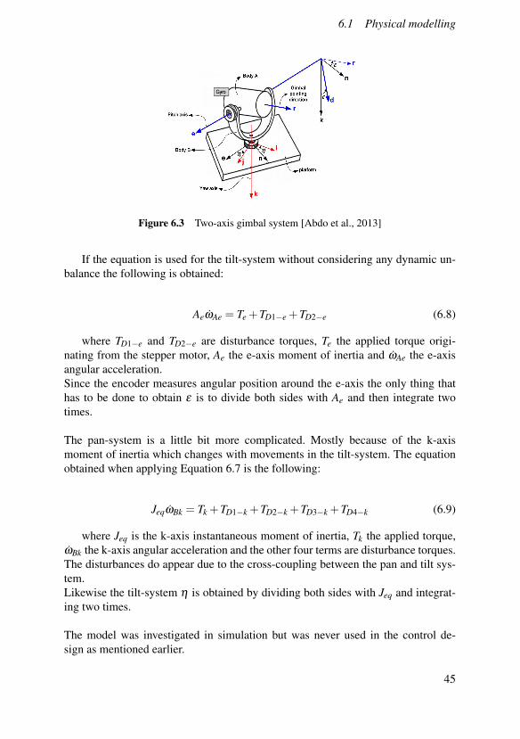
Figure 6.3 Two-axis gimbal system [Abdo et al., 2013]

If the equation is used for the tilt-system without considering any dynamic un-balance the following is obtained:

AeωAe = Te +TD1−e +TD2−e (6.8)

where TD1−e and TD2−e are disturbance torques, Te the applied torque origi-nating from the stepper motor, Ae the e-axis moment of inertia and ωAe the e-axisangular acceleration.Since the encoder measures angular position around the e-axis the only thing thathas to be done to obtain ε is to divide both sides with Ae and then integrate twotimes.

The pan-system is a little bit more complicated. Mostly because of the k-axismoment of inertia which changes with movements in the tilt-system. The equationobtained when applying Equation 6.7 is the following:

JeqωBk = Tk +TD1−k +TD2−k +TD3−k +TD4−k (6.9)

where Jeq is the k-axis instantaneous moment of inertia, Tk the applied torque,ωBk the k-axis angular acceleration and the other four terms are disturbance torques.The disturbances do appear due to the cross-coupling between the pan and tilt sys-tem.Likewise the tilt-system η is obtained by dividing both sides with Jeq and integrat-ing two times.

The model was investigated in simulation but was never used in the control de-sign as mentioned earlier.

45

Chapter 6. Modelling

6.2 System identification

System identification deals with the problem of creating dynamical models of sys-tems by investigating the relation between input and output signals. There are sev-eral methods for doing this, some more advanced than others. In some cases certainthings are already known about the system, for example physical constants. In othercases there are no knowledge about the system. In these cases black box models canbe created [Ljung, 2007]. This is the system identification approach that has beenapplied in this thesis.

Black box modelIn contrast to a physical model a black box model only describes the relationshipbetween the input signals and output signals of a system and does not care aboutthe underlying physics [Ljung and Glad, 2004]. There are several methods that canbe used to describe the relationship and the method used in this thesis is called stepresponse identification.

Step response identificationStep response analysis is a simple and frequently used method for analyzing howsignals affect each other. The idea of the method is to change all input signals atonce and then study how the output signals are affected [Ljung and Glad, 2004].The change of input signals, u(t), is done in the following way:

u(t) = u0, t < t0; u(t) = u1, t ≥ t0 (6.10)

Meaning that input signals gets the shape of a step. When investigating the effecton the output signals the following can be looked at:

• Time delays

• Static gain

• Character of response, e.g., oscillatory, damped etc.

In this thesis this kind of experiment has been done on two systems, pan andtilt, respectively. Moreover it was assumed that the two systems did not affect eachother meaning that two single-input-single-output (SISO) models were created.

To do the experiment a step generator was implemented in the camera software.The signal that was generated was the stepper motor speed signal, giving it theunit steps/s, and the output was measured with the gyroscope (rad/s). Due to thisthe experiment was carried out with the sensor frame in alignment with the chassiframe before starting the rotation. This was done to make sure that the gyroscopewould measure rotation around the pan- and tilt-axis, i.e., the k- and e-axis in Figure

46

6.2 System identification

6.3. The gyroscope was used instead of the encoder since it had a higher samplingrate.

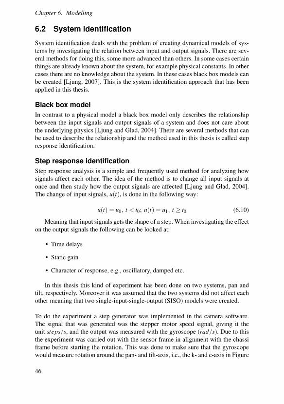
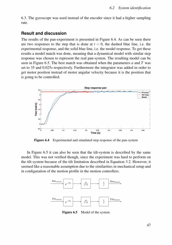
Result and discussionThe results of the pan-experiment is presented in Figure 6.4. As can be seen thereare two responses to the step that is done at t = 0, the dashed blue line, i.e. theexperimental response, and the solid blue line, i.e. the model response. To get theseresults a model match was done, meaning that a dynamical model with similar stepresponse was chosen to represent the real pan-system. The resulting model can beseen in Figure 6.5. The best match was obtained when the parameters a and T wasset to 35 and 0.025s respectively. Furthermore the integrator was added in order toget motor position instead of motor angular velocity because it is the position thatis going to be controlled.

0 0.05 0.1 0.15 0.2 0.25 0.3 0.35 0.4 0.45-0.5

0

0.5

1

1.5

2

2.5

3

3.5

Process

Ref step

Model

Step response pan

Time [s]

(seconds)

Ya

w [

rad

/s]

Figure 6.4 Experimental and simulated step response of the pan-system

In Figure 6.5 it can also be seen that the tilt-system is described by the samemodel. This was not verified though, since the experiment was hard to perform onthe tilt-system because of the tilt limitation described in Equation 3.2. However, itseemed like a reasonable assumption due to the similarities in mechanical setup andin configuration of the motion profile in the motion controllers.

e−T s as+a

1s

as+ae−T s 1

s

Panvelocity PanPosition

Tiltvelocity TiltPosition

Figure 6.5 Model of the system

47

Chapter 6. Modelling

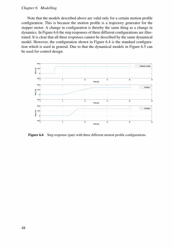
Note that the models described above are valid only for a certain motion profileconfiguration. This is because the motion profile is a trajectory generator for thestepper motor. A change in configuration is thereby the same thing as a change indynamics. In Figure 6.6 the step responses of three different configurations are illus-trated. It is clear that all three responses cannot be described by the same dynamicalmodel. However, the configuration shown in Figure 6.4 is the standard configura-tion which is used in general. Due to that the dynamical models in Figure 6.5 canbe used for control design.

0 5 10 15 20 25

Time [s]

-500

0

500

1000

Ya

w [°/s

]

Original config

0 5 10 15 20 25

Time [s]

-500

0

500

1000

Ya

w [°/s

]

Config 1

0 5 10 15 20 25

Time [s]

-500

0

500

1000

Ya

w [°/s

]

Config 2

Figure 6.6 Step response (pan) with three different motion profile configurations

48

7Trajectory generation

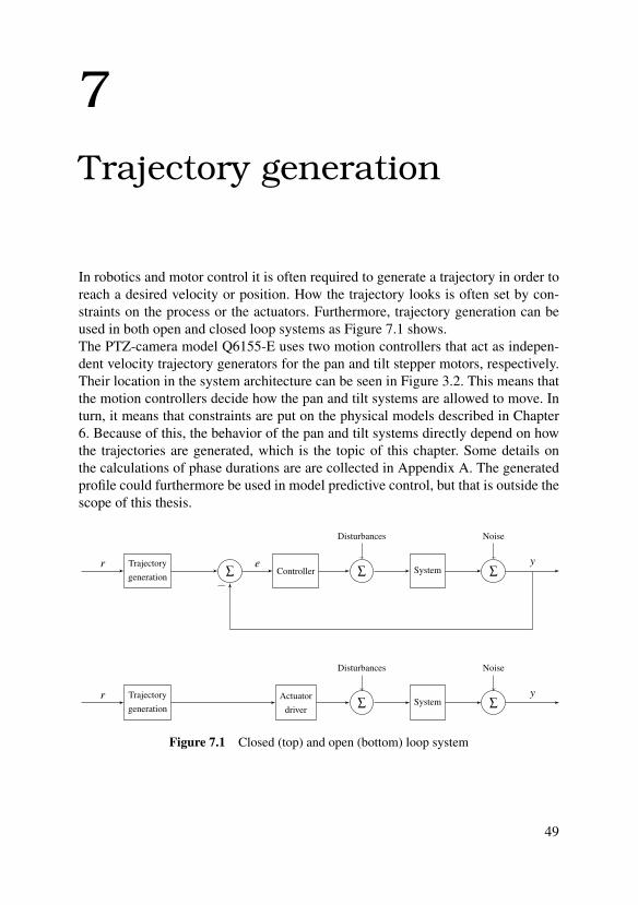
In robotics and motor control it is often required to generate a trajectory in order toreach a desired velocity or position. How the trajectory looks is often set by con-straints on the process or the actuators. Furthermore, trajectory generation can beused in both open and closed loop systems as Figure 7.1 shows.The PTZ-camera model Q6155-E uses two motion controllers that act as indepen-dent velocity trajectory generators for the pan and tilt stepper motors, respectively.Their location in the system architecture can be seen in Figure 3.2. This means thatthe motion controllers decide how the pan and tilt systems are allowed to move. Inturn, it means that constraints are put on the physical models described in Chapter6. Because of this, the behavior of the pan and tilt systems directly depend on howthe trajectories are generated, which is the topic of this chapter. Some details onthe calculations of phase durations are are collected in Appendix A. The generatedprofile could furthermore be used in model predictive control, but that is outside thescope of this thesis.

Trajectorygeneration ∑ Controller ∑

Disturbances

System ∑

Noise

∑

Disturbances

Actuatordriver

System ∑

Noise

Trajectorygeneration

r e y

−

r y

Figure 7.1 Closed (top) and open (bottom) loop system

49

Chapter 7. Trajectory generation

7.1 Motion profiles

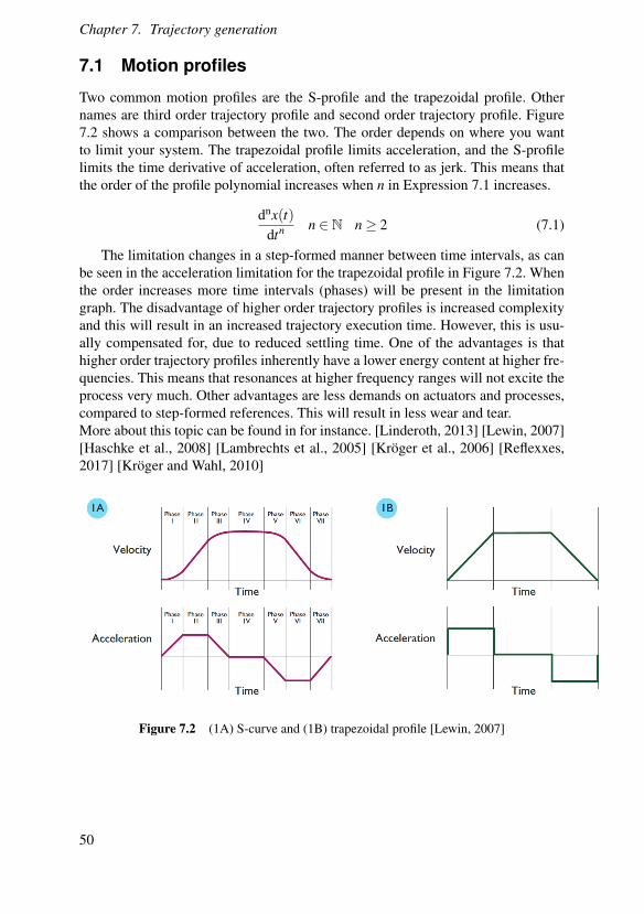
Two common motion profiles are the S-profile and the trapezoidal profile. Othernames are third order trajectory profile and second order trajectory profile. Figure7.2 shows a comparison between the two. The order depends on where you wantto limit your system. The trapezoidal profile limits acceleration, and the S-profilelimits the time derivative of acceleration, often referred to as jerk. This means thatthe order of the profile polynomial increases when n in Expression 7.1 increases.

dnx(t)dtn n ∈ N n≥ 2 (7.1)

The limitation changes in a step-formed manner between time intervals, as canbe seen in the acceleration limitation for the trapezoidal profile in Figure 7.2. Whenthe order increases more time intervals (phases) will be present in the limitationgraph. The disadvantage of higher order trajectory profiles is increased complexityand this will result in an increased trajectory execution time. However, this is usu-ally compensated for, due to reduced settling time. One of the advantages is thathigher order trajectory profiles inherently have a lower energy content at higher fre-quencies. This means that resonances at higher frequency ranges will not excite theprocess very much. Other advantages are less demands on actuators and processes,compared to step-formed references. This will result in less wear and tear.More about this topic can be found in for instance. [Linderoth, 2013] [Lewin, 2007][Haschke et al., 2008] [Lambrechts et al., 2005] [Kröger et al., 2006] [Reflexxes,2017] [Kröger and Wahl, 2010]

Figure 7.2 (1A) S-curve and (1B) trapezoidal profile [Lewin, 2007]

50

7.1 Motion profiles

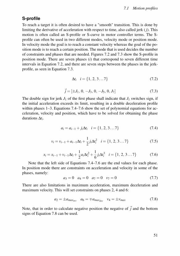
S-profileTo reach a target it is often desired to have a "smooth" transition. This is done bylimiting the derivative of acceleration with respect to time, also called jerk ( j). Thismotion is often called an S-profile or S-curve in motor controller terms. The S-profile can often be used in two different modes, velocity mode or position mode.In velocity mode the goal is to reach a constant velocity whereas the goal of the po-sition mode is to reach a certain position. The mode that is used decides the numberof constraints and phases that are needed. Figures 7.2 and 7.3 show the S-profile inposition mode. There are seven phases (i) that correspond to seven different timeintervals in Equation 7.2, and there are seven steps between the phases in the jerk-profile, as seen in Equation 7.3.

∆ti i = 1, 2, 3 . . .7 (7.2)

~j = [±J1, 0, −J3, 0, −J5, 0, J7] (7.3)

The double sign for jerk J1 of the first phase shall indicate that J1 switches sign, ifthe initial acceleration exceeds its limit, resulting in a double deceleration profilewithin phases 1–3. Equations 7.4–7.6 show the set of polynomial equations for ac-celeration, velocity and position, which have to be solved for obtaining the phasedurations ∆ti.

ai = ai−1 + ji∆ti i = 1, 2, 3 . . .7 (7.4)

vi = vi−1 +ai−1∆ti +12

ji∆t2i i = 1, 2, 3 . . .7 (7.5)

xi = xi−1 + vi−1∆ti +12

ai∆t2i +

16

ji∆t3i i = 1, 2, 3 . . .7 (7.6)

Note that the left side of Equations 7.4–7.6 are the end values for each phase.In position mode there are constraints on acceleration and velocity in some of thephases, namely:

a3 = 0 a4 = 0 a7 = 0 v7 = 0 (7.7)

There are also limitations in maximum acceleration, maximum deceleration andmaximum velocity. This will set constraints on phases 2, 4 and 6:

a2 =±amaxacc a6 =∓amaxdec v4 =±vmax (7.8)

Note, that in order to calculate negative position the negative of ~j and the bottomsigns of Equation 7.8 can be used.

51

Chapter 7. Trajectory generation

0 2 4 6 8 10 12 14 16 18

Time [s]

-5

0

5

j(t) [m

/s

3]

S-profile

0 2 4 6 8 10 12 14 16 18

Time [s]

-10

0

10

a(t) [m

/s

2]

0 2 4 6 8 10 12 14 16 18

Time [s]

0

20

40

v(t) [m

/s]

0 2 4 6 8 10 12 14 16 18

Time [s]

0

200

400

x(t) [m

]

Figure 7.3 An example of a S-profile in position mode

In velocity mode only three phases are needed in order to reach the target ve-locity. This means that there are just three phase durations and jerk-profile steps, asseen in Equations 7.9–7.10. Moreover, Equations 7.4–7.6 can be used to calculateacceleration, velocity and position for the three phases. Equation 7.11 shows theconstraints and limits that are needed.

∆ti i = 1, 2, 3 (7.9)

~j = [±J1, 0, −J3] (7.10)

a2 =±amaxacc a3 = 0 (7.11)

52

7.2 Motion controllers

7.2 Motion controllers

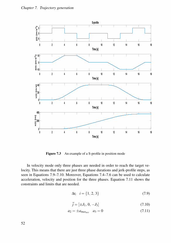
Axis uses the motion controller chip TMC4361A-LA from Trinamic and it is usedfor controlling the stepper motors [Trinamic, 2017]. The chip has capability to gen-erate both S-profiles and trapezoidal profiles. The current configuration is S-profilemotion and both the pan and tilt system are equipped with a motion controller inan open loop configuration as Figure 7.4 shows. However, the encoders are used tocorrect the position after a movement has been carried out. Moreover, the motioncontrollers can be used in both velocity and position mode.

Figure 7.4 An open loop case with TMC4361A-LA [Trinamic, 2017]

In this thesis the motion controllers have been used in velocity mode for boththe pan and tilt system. The jerk profile was not changed because it was already op-timized for Axis’ needs. This means that all phases in the jerk-profile are different,as seen in Equation 7.12.

J1 6= J3 6= J5 6= J7 (7.12)

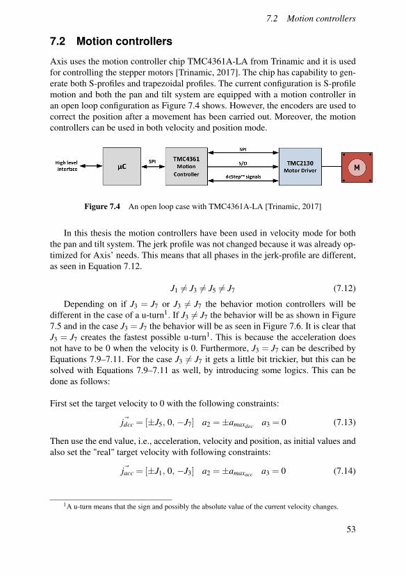
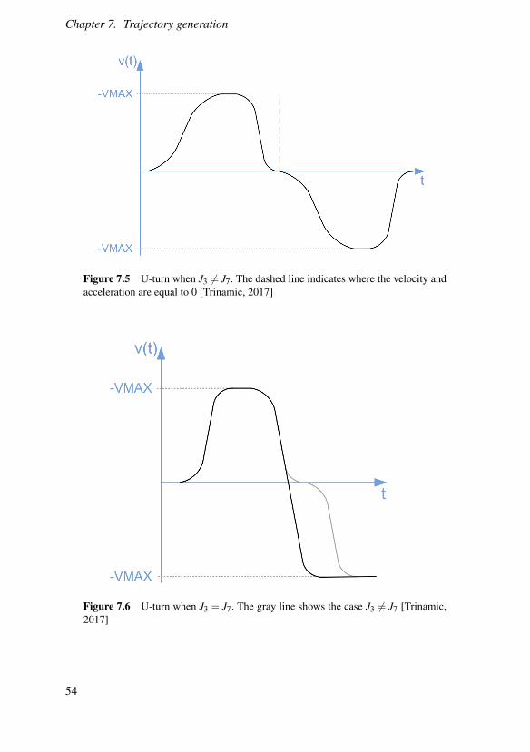
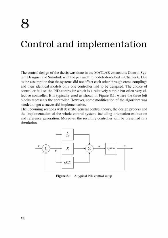
Depending on if J3 = J7 or J3 6= J7 the behavior motion controllers will bedifferent in the case of a u-turn1. If J3 6= J7 the behavior will be as shown in Figure7.5 and in the case J3 = J7 the behavior will be as seen in Figure 7.6. It is clear thatJ3 = J7 creates the fastest possible u-turn1. This is because the acceleration doesnot have to be 0 when the velocity is 0. Furthermore, J3 = J7 can be described byEquations 7.9–7.11. For the case J3 6= J7 it gets a little bit trickier, but this can besolved with Equations 7.9–7.11 as well, by introducing some logics. This can bedone as follows:

First set the target velocity to 0 with the following constraints:

~jdcc = [±J5, 0, −J7] a2 =±amaxdec a3 = 0 (7.13)

Then use the end value, i.e., acceleration, velocity and position, as initial values andalso set the "real" target velocity with following constraints:

~jacc = [±J1, 0, −J3] a2 =±amaxacc a3 = 0 (7.14)

1A u-turn means that the sign and possibly the absolute value of the current velocity changes.

53

Chapter 7. Trajectory generation

Figure 7.5 U-turn when J3 6= J7. The dashed line indicates where the velocity andacceleration are equal to 0 [Trinamic, 2017]

Figure 7.6 U-turn when J3 = J7. The gray line shows the case J3 6= J7 [Trinamic,2017]

54

7.3 Discussion

7.3 Discussion

When using a desired motion profile like the S-curve for the reference the problemis to calculate the ∆ti, representing how long each phase is, based on the limits foracceleration, velocity and jerk. Moreover, the initial values are known, i.e., a0, v0and x0. The mode that is used will affect the complexity, i.e., the position moderesults in more phases, limits and constraints compared to the velocity mode. Asmentioned earlier, the velocity mode was used and in Appendix A a more detailedcalculation of ∆ti is provided. The motion controllers add additional complexitydepending on which of the cases J3 = J7 or J3 6= J7 that is used. For the latter case,logics can be added to the calculations done in Appendix A. If the motion controllerbehavior would have been used in the control design, a better controller performancehad most certainly been obtained.

55

8Control and implementation

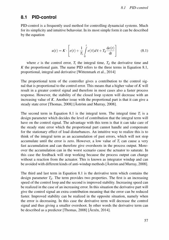
The control design of the thesis was done in the MATLAB extensions Control Sys-tem Designer and Simulink with the pan and tilt models described in Chapter 6. Dueto the assumption that the systems did not affect each other through cross-couplingsand their identical models only one controller had to be designed. The choice ofcontroller fell on the PID-controller which is a relatively simple but often very ef-fective controller. It is typically used as shown in Figure 8.1, where the three leftblocks represents the controller. However, some modification of the algorithm wasneeded to get a successful implementation.The upcoming sections will describe general control theory, the design process andthe implementation of the whole control system, including orientation estimationand reference generation. Moreover the resulting controller will be presented in asimulation.

∑ K

KTis

sKTd

∑ Systemr

eu y

−

Figure 8.1 A typical PID control setup

56

8.1 PID-control

8.1 PID-control

PID-control is a frequently used method for controlling dynamcial systems. Muchfor its simplicity and intuitive behavoiur. In its most simple form it can be describedby the equation

u(t) = K ·

[e(t)+

1Ti

t∫0

e(τ)dτ +Tdde(t)

dt

](8.1)

where e is the control error, Ti the integral time, Td the derivative time andK the proportional gain. The name PID refers to the three terms in Equation 8.1,proportional, integral and derivative [Wittenmark et al., 2014]

The proportional term of the controller gives a contribution to the control sig-nal that is proportional to the control error. This means that a higher value of K willresult in a greater control signal and therefore in most cases also a faster processresponse. However, the stability of the closed loop system will decrease with anincreasing value of K. Another issue with the proportional part is that it can give asteady state error [Thomas, 2008] [Åström and Murray, 2008].

The second term in Equation 8.1 is the integral term. The integral time Ti is adesign parameter which decides the level of contribution that the integral term willhave on the control signal. The advantage with this term is that it can take care ofthe steady state error which the proportional part cannot handle and compensatefor the stationary effect of load disturbances. An intuitive way to realize this is tothink of the integral term as an accumulation of past errors, which will not stopaccumulate until the error is zero. However, a low value of Ti can cause a veryfast accumulation and can therefore give overshoots in the process output. More-over the accumulation can in the worst scenario cause the actuator to saturate. Inthis case the feedback will stop working because the process output can changewithout a reaction from the actuator. This is known as integrator windup and canbe avoided with different kinds of anti-windup methods [Åström and Murray, 2008].

The third and last term in Equation 8.1 is the derivative term which contains thedesign parameter Td . The term provides two properties. The first is an increasingspeed of the control loop and the second is improved stability. Increasing speed canbe realized in the case of an increasing error. In this situation the derivative part willgive the control signal an extra contribution meaning that the error can be reducedfaster. Improved stability can be realized in the opposite situation, namely whenthe error is decreasing. In this case the derivative term will decrease the controlsignal and thus giving a smaller overshoot. In other words the derivative term canbe described as a predictor [Thomas, 2008] [Årzén, 2014].

57

Chapter 8. Control and implementation

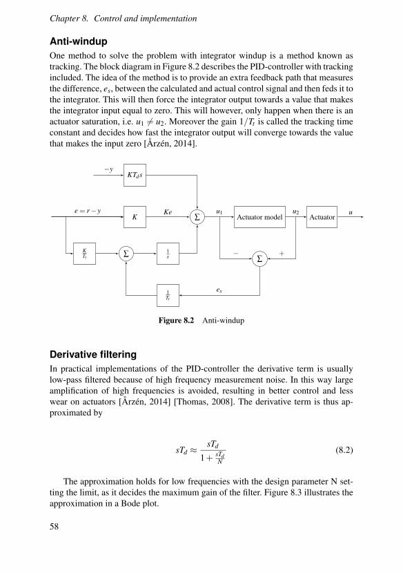
Anti-windupOne method to solve the problem with integrator windup is a method known astracking. The block diagram in Figure 8.2 describes the PID-controller with trackingincluded. The idea of the method is to provide an extra feedback path that measuresthe difference, es, between the calculated and actual control signal and then feds it tothe integrator. This will then force the integrator output towards a value that makesthe integrator input equal to zero. This will however, only happen when there is anactuator saturation, i.e. u1 6= u2. Moreover the gain 1/Tt is called the tracking timeconstant and decides how fast the integrator output will converge towards the valuethat makes the input zero [Årzén, 2014].

KTds

K ∑Ke

1s∑

Actuator model Actuator

∑

1Tt

KTi

u1 u2

− +

−y

e = r− y u

es

Figure 8.2 Anti-windup

Derivative filteringIn practical implementations of the PID-controller the derivative term is usuallylow-pass filtered because of high frequency measurement noise. In this way largeamplification of high frequencies is avoided, resulting in better control and lesswear on actuators [Årzén, 2014] [Thomas, 2008]. The derivative term is thus ap-proximated by

sTd ≈sTd

1+ sTdN

(8.2)

The approximation holds for low frequencies with the design parameter N set-ting the limit, as it decides the maximum gain of the filter. Figure 8.3 illustrates theapproximation in a Bode plot.

58

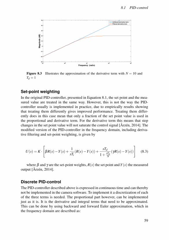
8.1 PID-control

10-1

100

101

102

103

-30

-20

-10

0

10

20

30

40

50

Ma

gn

itu

de

(d

B)

Unfiltered derivative term

Filtered derivative term

Frequency (rad/s)

Figure 8.3 Illustrates the approximation of the derivative term with N = 10 andTd = 1

Set-point weightingIn the original PID-controller, presented in Equation 8.1, the set point and the mea-sured value are treated in the same way. However, this is not the way the PID-controller usually is implemented in practice, due to empirically results showingthat treating them differently gives improved performance. Treating them differ-ently does in this case mean that only a fraction of the set point value is used inthe proportional and derivative term. For the derivative term this means that stepchanges in the set point value will not saturate the control signal [Årzén, 2014]. Themodified version of the PID-controller in the frequency domain, including deriva-tive filtering and set-point weighting, is given by

U(s) = K ·

[βR(s)−Y (s)+

1sTi

(R(s)−Y (s))+sTd

1+ sTdN

(γR(s)−Y (s))

](8.3)

where β and γ are the set-point weights, R(s) the set point and Y (s) the measuredoutput [Årzén, 2014].

Discrete PID-controlThe PID-controller described above is expressed in continuous time and can therebynot be implemented in the camera software. To implement it a discretization of eachof the three terms is needed. The proportional part however, can be implementedjust as it is. It is the derivative and integral terms that need to be approximated.This can be done by using backward and forward Euler approximation, which inthe frequency domain are described as:

59

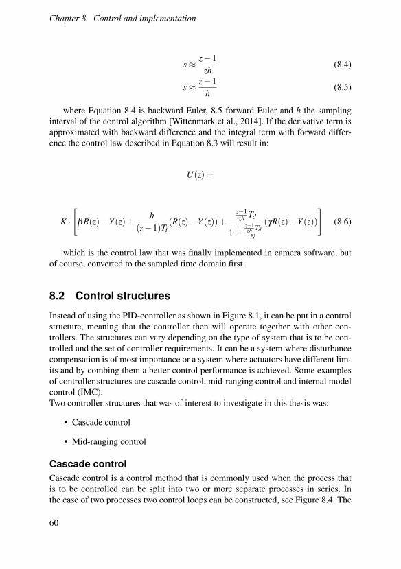
Chapter 8. Control and implementation

s≈ z−1zh

(8.4)

s≈ z−1h

(8.5)

where Equation 8.4 is backward Euler, 8.5 forward Euler and h the samplinginterval of the control algorithm [Wittenmark et al., 2014]. If the derivative term isapproximated with backward difference and the integral term with forward differ-ence the control law described in Equation 8.3 will result in:

U(z) =

K ·

[βR(z)−Y (z)+

h(z−1)Ti

(R(z)−Y (z))+z−1zh Td

1+z−1zh TdN

(γR(z)−Y (z))

](8.6)

which is the control law that was finally implemented in camera software, butof course, converted to the sampled time domain first.

8.2 Control structures

Instead of using the PID-controller as shown in Figure 8.1, it can be put in a controlstructure, meaning that the controller then will operate together with other con-trollers. The structures can vary depending on the type of system that is to be con-trolled and the set of controller requirements. It can be a system where disturbancecompensation is of most importance or a system where actuators have different lim-its and by combing them a better control performance is achieved. Some examplesof controller structures are cascade control, mid-ranging control and internal modelcontrol (IMC).Two controller structures that was of interest to investigate in this thesis was:

• Cascade control

• Mid-ranging control

Cascade controlCascade control is a control method that is commonly used when the process thatis to be controlled can be split into two or more separate processes in series. Inthe case of two processes two control loops can be constructed, see Figure 8.4. The

60

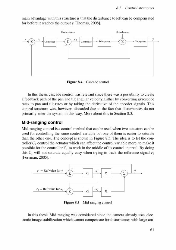
8.2 Control structures

main advantage with this structure is that the disturbance to left can be compensatedfor before it reaches the output y [Thomas, 2008].

∑ Controller ∑

Disturbances

Controller Subsystem ∑

Disturbances

Subsystemr e1 e2

−

y

−

Figure 8.4 Cascade control

In this thesis cascade control was relevant since there was a possibility to createa feedback path of the pan and tilt angular velocity. Either by converting gyroscoperates to pan and tilt rates or by taking the derivative of the encoder signals. Thiscontrol structure was, however, discarded due to the fact that disturbances do notprimarily enter the system in this way. More about this in Section 8.3.

Mid-ranging controlMid-ranging control is a control method that can be used when two actuators can beused for controlling the same control variable but one of them is easier to saturatethan the other one. The concept is shown in Figure 8.5. The idea is to let the con-troller C2 control the actuator which can affect the control variable more, to make itpossible for the controller C1 to work in the middle of its control interval. By doingthis C1 will not saturate equally easy when trying to track the reference signal r1[Forsman, 2005].

∑ C1 P1 ∑

P2C2∑

r1 = Ref value for y u1− y

r2 = Ref value for u1 u2

Figure 8.5 Mid-ranging control

In this thesis Mid-ranging was considered since the camera already uses elec-tronic image stabilization which cannot compensate for disturbances with large am-

61

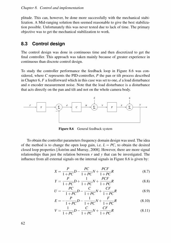
Chapter 8. Control and implementation

plitude. This can, however, be done more successfully with the mechanical stabi-lization. A Mid-ranging solution then seemed reasonable to give the best stabiliza-tion possible. Unfortunately this was never tested due to lack of time. The primaryobjective was to get the mechanical stabilization to work.

8.3 Control design

The control design was done in continuous time and then discretized to get thefinal controller. This approach was taken mainly because of greater experience incontinuous than discrete control design.

To study the controller performance the feedback loop in Figure 8.6 was con-sidered, where C represents the PID-controller, P the pan or tilt process describedin Chapter 6, F a feedforward which in this case was set to one, d a load disturbanceand n encoder measurement noise. Note that the load disturbance is a disturbancethat acts directly on the pan and tilt and not on the whole camera body.

F ∑ C ∑

d

P ∑

n

r e u v x y

−

Figure 8.6 General feedback system

To obtain the controller parameters frequency domain design was used. The ideaof the method is to change the open loop gain, i.e. L = PC, to obtain the desiredclosed loop properties [Åström and Murray, 2008]. However, there are more signalrelationships than just the relation between r and y that can be investigated. Theinfluence from all external signals on the internal signals in Figure 8.6 is given by:

X =P

1+PCD− PC

1+PCN +

PCF1+PC

R (8.7)

Y =P

1+PCD+

11+PC

N +PCF

1+PCR (8.8)

U =− PC1+PC

D− C1+PC

N +CF

1+PCR (8.9)

E =− P1+PC

D− 11+PC

N +F

1+PCR (8.10)

V =1

1+PCD− C

1+PCN +

CF1+PC

R (8.11)

62

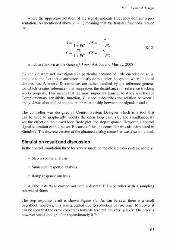
8.3 Control design

where the uppercase notation of the signals indicate frequency domain repre-sentation. As mentioned above F = 1, meaning that the transfer functions reduceto:

S =1

1+PCPS =

P1+PC

T =PC

1+PCCS =

C1+PC

(8.12)

which are known as the Gang o f Four [Åström and Murray, 2008].

CS and PS were not investigated in particular because of little encoder noise, n,and due to the fact that disturbances mostly do not enter the system where the loaddisturbance, d, enters. Disturbances are rather handled by the reference genera-tor which creates references that suppresses the disturbances if reference trackingworks properly. This means that the most important transfer to study was the theComplementary sensitivity function, T , since it describes the relation between rand y. S was also studied to look at the relationship between the signals r and e.

The controller was designed in Control System Designer which is a tool thatcan be used to graphically modify the open loop gain, PC, and simultaneouslysee the effect on the closed loop Bode plot and step response. However, a controlsignal saturation cannot be set. Because of this the controller was also simulated inSimulink. The discrete version of the obtained analog controller was also simulated.

Simulation result and discussionIn the control simulation three tests were made on the closed loop system, namely:

• Step response analysis

• Sinusoidal response analysis

• Ramp response analysis

All the tests were carried out with a discrete PID-controller with a samplinginterval of 50ms.

The step response result is shown Figure 8.7. As can be seen there is a smallovershoot, however, this was accepted due to reduction of rise time. Moreover itcan be seen that the error converges towards zero but not very quickly. The error ishowever small enough after approximately 0.7s.

63

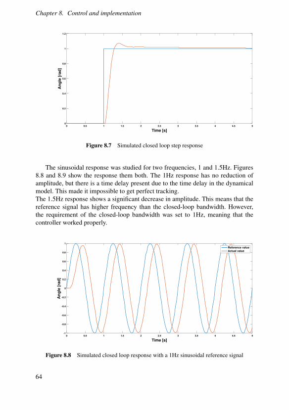
Chapter 8. Control and implementation

0 0.5 1 1.5 2 2.5 3 3.5 4 4.5 5

Time [s]

0

0.2

0.4

0.6

0.8

1

1.2

An

gle

[ra

d]

Figure 8.7 Simulated closed loop step response

The sinusoidal response was studied for two frequencies, 1 and 1.5Hz. Figures8.8 and 8.9 show the response them both. The 1Hz response has no reduction ofamplitude, but there is a time delay present due to the time delay in the dynamicalmodel. This made it impossible to get perfect tracking.The 1.5Hz response shows a significant decrease in amplitude. This means that thereference signal has higher frequency than the closed-loop bandwidth. However,the requirement of the closed-loop bandwidth was set to 1Hz, meaning that thecontroller worked properly.

0 0.5 1 1.5 2 2.5 3 3.5 4 4.5 5

Time [s]

-1

-0.8

-0.6

-0.4

-0.2

0

0.2

0.4

0.6

0.8

1

An

gle

[ra

d]

Reference value

Actual value

Figure 8.8 Simulated closed loop response with a 1Hz sinusoidal reference signal

64

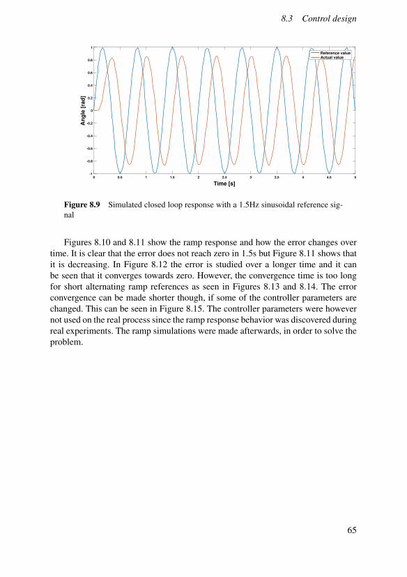
8.3 Control design

0 0.5 1 1.5 2 2.5 3 3.5 4 4.5 5

Time [s]

-1

-0.8

-0.6

-0.4

-0.2

0

0.2

0.4

0.6

0.8

1

An

gle

[ra

d]

Reference valueActual value

Figure 8.9 Simulated closed loop response with a 1.5Hz sinusoidal reference sig-nal

Figures 8.10 and 8.11 show the ramp response and how the error changes overtime. It is clear that the error does not reach zero in 1.5s but Figure 8.11 shows thatit is decreasing. In Figure 8.12 the error is studied over a longer time and it canbe seen that it converges towards zero. However, the convergence time is too longfor short alternating ramp references as seen in Figures 8.13 and 8.14. The errorconvergence can be made shorter though, if some of the controller parameters arechanged. This can be seen in Figure 8.15. The controller parameters were howevernot used on the real process since the ramp response behavior was discovered duringreal experiments. The ramp simulations were made afterwards, in order to solve theproblem.

65

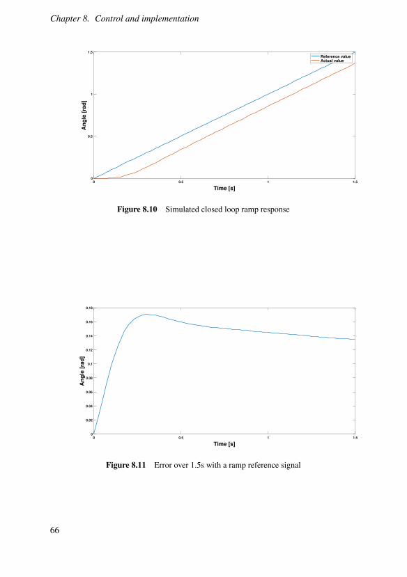
Chapter 8. Control and implementation

0 0.5 1 1.5

Time [s]

0

0.5

1

1.5

An

gle

[ra

d]

Reference valueActual value

Figure 8.10 Simulated closed loop ramp response

0 0.5 1 1.5

Time [s]

0

0.02

0.04

0.06

0.08

0.1

0.12

0.14

0.16

0.18

An

gle

[ra

d]

Figure 8.11 Error over 1.5s with a ramp reference signal

66

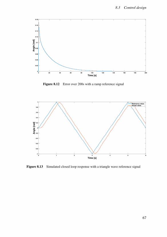
8.3 Control design

0 20 40 60 80 100 120 140 160 180 200

Time [s]

0

0.02

0.04

0.06

0.08

0.1

0.12

0.14

0.16

0.18

An

gle

[ra

d]

Figure 8.12 Error over 200s with a ramp reference signal

0 1 2 3 4 5 6

Time [s]

-1

-0.8

-0.6

-0.4

-0.2

0

0.2

0.4

0.6

0.8

1

An

gle

[ra

d]

Reference valueActual value

Figure 8.13 Simulated closed loop response with a triangle wave reference signal

67

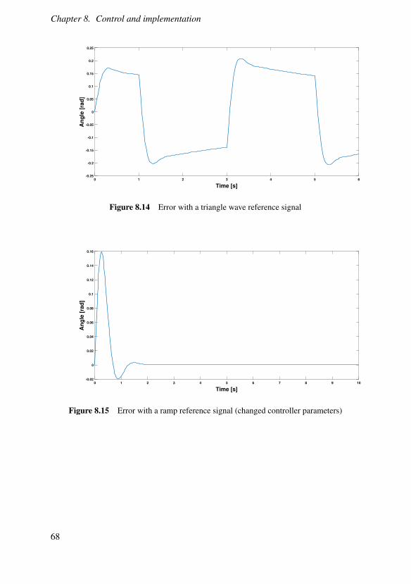
Chapter 8. Control and implementation

0 1 2 3 4 5 6

Time [s]

-0.25

-0.2

-0.15

-0.1

-0.05

0

0.05

0.1

0.15

0.2

0.25

An

gle

[ra

d]

Figure 8.14 Error with a triangle wave reference signal

0 1 2 3 4 5 6 7 8 9 10

Time [s]

-0.02

0

0.02

0.04

0.06

0.08

0.1

0.12

0.14

0.16

An

gle

[ra

d]

Figure 8.15 Error with a ramp reference signal (changed controller parameters)

68

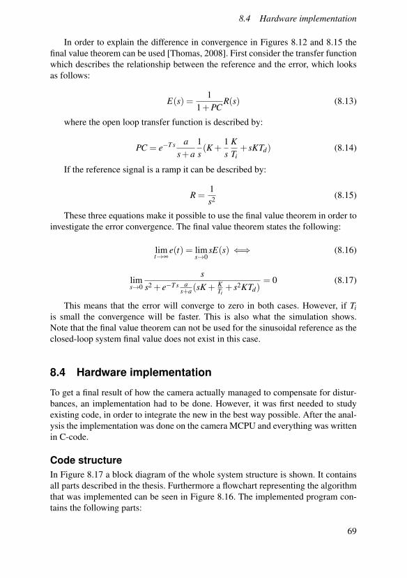
8.4 Hardware implementation

In order to explain the difference in convergence in Figures 8.12 and 8.15 thefinal value theorem can be used [Thomas, 2008]. First consider the transfer functionwhich describes the relationship between the reference and the error, which looksas follows:

E(s) =1

1+PCR(s) (8.13)

where the open loop transfer function is described by:

PC = e−T s as+a

1s(K +

1s

KTi+ sKTd) (8.14)

If the reference signal is a ramp it can be described by:

R =1s2 (8.15)

These three equations make it possible to use the final value theorem in order toinvestigate the error convergence. The final value theorem states the following:

limt→∞

e(t) = lims→0

sE(s) ⇐⇒ (8.16)

lims→0

ss2 + e−T s a

s+a (sK + KTi+ s2KTd)

= 0 (8.17)

This means that the error will converge to zero in both cases. However, if Tiis small the convergence will be faster. This is also what the simulation shows.Note that the final value theorem can not be used for the sinusoidal reference as theclosed-loop system final value does not exist in this case.

8.4 Hardware implementation

To get a final result of how the camera actually managed to compensate for distur-bances, an implementation had to be done. However, it was first needed to studyexisting code, in order to integrate the new in the best way possible. After the anal-ysis the implementation was done on the camera MCPU and everything was writtenin C-code.

Code structureIn Figure 8.17 a block diagram of the whole system structure is shown. It containsall parts described in the thesis. Furthermore a flowchart representing the algorithmthat was implemented can be seen in Figure 8.16. The implemented program con-tains the following parts:

69

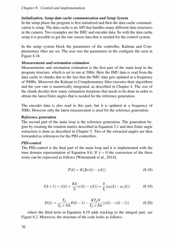
Chapter 8. Control and implementation

Initialization, Setup data cache communication and Setup SystemIn the setup phase the program is first initialized and then the data cache communi-cation is setup. The data cache is an API that handles many different data structuresin the camera. Two examples are the IMU and encoder data. So with the data cachesetup it is possible to get the raw sensor data that is needed for the control system.

In the setup system block the parameters of the controller, Kalman and Com-plementary filter are set. The user sets the parameters in the configure file seen inFigure 8.16.

Measurements and orientation estimationMeasurements and orientation estimation is the first part of the main loop in theprogram structure, which is set to run at 20Hz. Here the IMU data is read from thedata cache in chunks due to the fact that the IMU data gets updated at a frequencyof 500Hz. Moreover the Kalman or Complementary filter executes their algorithmsand the yaw rate is numerically integrated, as described in Chapter 4. The size ofthe chunk decides how many estimation iterations that needs to be done in order toobtain the latest Euler angles that is needed for the reference generation.

The encoder data is also read in this part, but it is updated at a frequency of50Hz. However only the latest measurement is used for the reference generation.

Reference generationThe second part of the main loop is the reference generation. The generation be-gins by creating the rotation matrix described in Equation 5.1 and then Euler angleextraction is done as described in Chapter 5. Two of the extracted angles are thenforwarded as references for the PID-controllers.

PID-controlThe PID-control is the final part of the main loop and it is implemented with thetime domain representation of Equation 8.6. If γ = 0 the conversion of the threeterms can be expressed as follows [Wittenmark et al., 2014]:

P(k) = K(β r(k)− y(k)) (8.18)

I(k+1) = I(k)+KhTi

(r(k)− y(k))+hTt(u2(k)−u1(k)) (8.19)

D(k) =Td

Td +NhD(k−1)− KTdN

Td +Nh(y(k)− y(k−1)) (8.20)

where the third term in Equation 8.19 adds tracking to the integral part, seeFigure 8.2. Moreover, the structure of the code looks as follows:

70

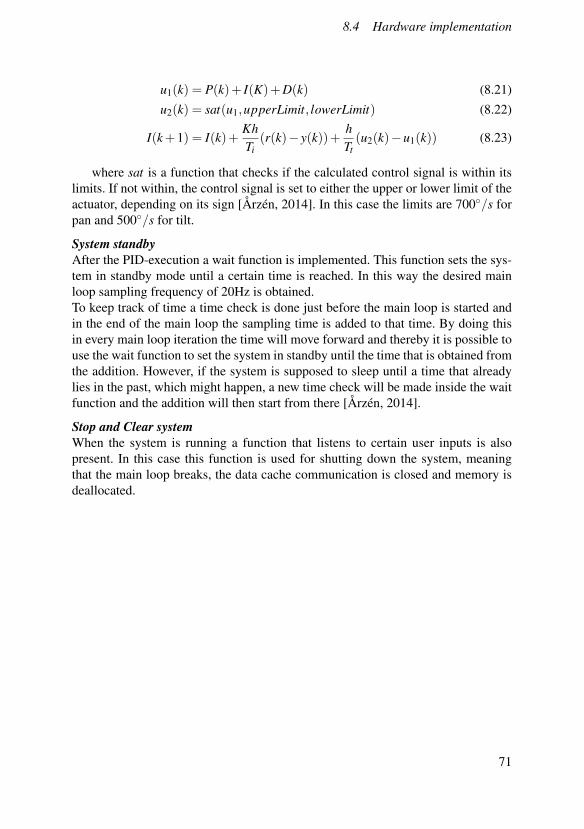
8.4 Hardware implementation

u1(k) = P(k)+ I(K)+D(k) (8.21)u2(k) = sat(u1,upperLimit, lowerLimit) (8.22)

I(k+1) = I(k)+KhTi

(r(k)− y(k))+hTt(u2(k)−u1(k)) (8.23)

where sat is a function that checks if the calculated control signal is within itslimits. If not within, the control signal is set to either the upper or lower limit of theactuator, depending on its sign [Årzén, 2014]. In this case the limits are 700/s forpan and 500/s for tilt.

System standbyAfter the PID-execution a wait function is implemented. This function sets the sys-tem in standby mode until a certain time is reached. In this way the desired mainloop sampling frequency of 20Hz is obtained.To keep track of time a time check is done just before the main loop is started andin the end of the main loop the sampling time is added to that time. By doing thisin every main loop iteration the time will move forward and thereby it is possible touse the wait function to set the system in standby until the time that is obtained fromthe addition. However, if the system is supposed to sleep until a time that alreadylies in the past, which might happen, a new time check will be made inside the waitfunction and the addition will then start from there [Årzén, 2014].

Stop and Clear systemWhen the system is running a function that listens to certain user inputs is alsopresent. In this case this function is used for shutting down the system, meaningthat the main loop breaks, the data cache communication is closed and memory isdeallocated.

71

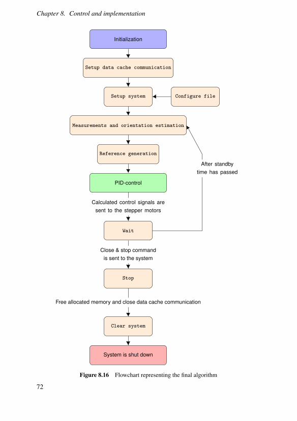
Chapter 8. Control and implementation

Initialization

Setup data cache communication

Setup system

Measurements and orientation estimation

Reference generation

PID-control

Wait

Stop

Clear system

Configure file

System is shut down

Calculated control signals aresent to the stepper motors

Close & stop commandis sent to the system

Free allocated memory and close data cache communication

After standbytime has passed

Figure 8.16 Flowchart representing the final algorithm

72

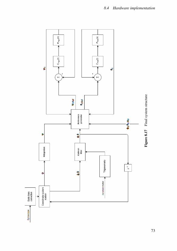
8.4 Hardware implementation

Figu

re8.

17Fi

nals

yste

mst

ruct

ure

73

9Results

The implementation made it possible to carry out experiments on the real pro-cess/camera and compare it with the simulation results. However, the experimentswere carried out for both pan and tilt, which was not necessary in the simulation.The following experiments were done:

• Closed loop step response

• Closed loop sinusoidal response

• Shake experiments

9.1 Closed loop step response

The results of the step response experiments can be seen in Figures 9.1 - 9.3. Notethat the simulated response is also present.

Both the pan and tilt experiment differ in overshoot compared to the simulation, seeFigures 9.1 and 9.2. However, the model seems to describe the system good enoughfor these cases.In Figure 9.3 though, it can be seen that the tilt overshoot varies depending onstep magnitude. This indicates that there is a nonlinearity present in the tilt system.Hence a linear time invariant model might not be good enough in all cases. Thiswas however never investigated in depth due to lack of time.

74

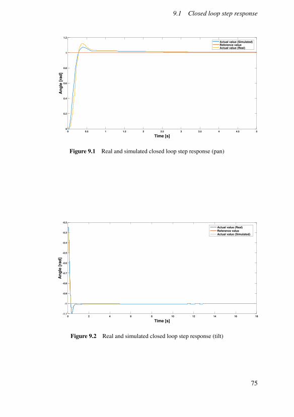
9.1 Closed loop step response

0 0.5 1 1.5 2 2.5 3 3.5 4 4.5 5

Time [s]

0

0.2

0.4

0.6

0.8

1

1.2

An

gle

[ra

d]

Actual value (Simulated)Reference valueActual value (Real)

Figure 9.1 Real and simulated closed loop step response (pan)

0 2 4 6 8 10 12 14 16 18

Time [s]

-1.1

-1

-0.9

-0.8

-0.7

-0.6

-0.5

-0.4

-0.3

-0.2

An

gle

[ra

d]

Actual value (Real)

Reference value

Actual value (Simulated)

Figure 9.2 Real and simulated closed loop step response (tilt)

75

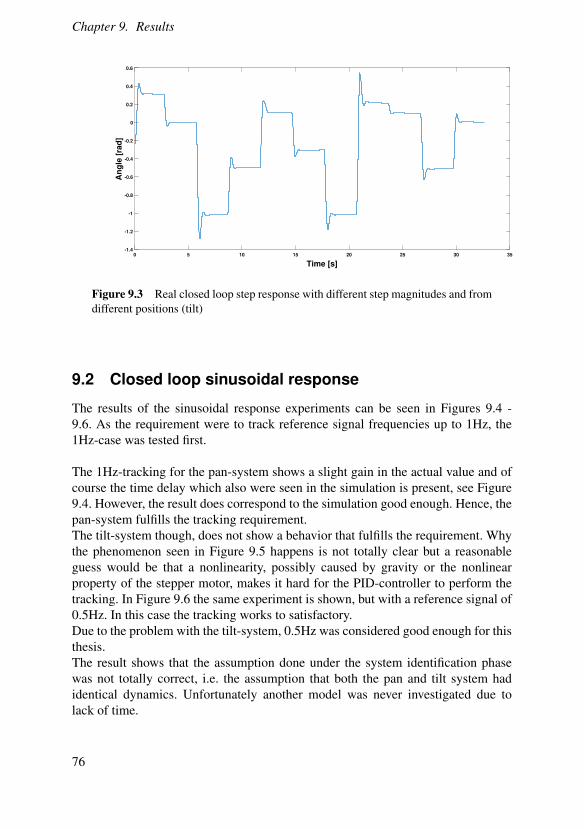
Chapter 9. Results

0 5 10 15 20 25 30 35

Time [s]

-1.4

-1.2

-1

-0.8

-0.6

-0.4

-0.2

0

0.2

0.4

0.6

An

gle

[ra

d]

Figure 9.3 Real closed loop step response with different step magnitudes and fromdifferent positions (tilt)

9.2 Closed loop sinusoidal response

The results of the sinusoidal response experiments can be seen in Figures 9.4 -9.6. As the requirement were to track reference signal frequencies up to 1Hz, the1Hz-case was tested first.

The 1Hz-tracking for the pan-system shows a slight gain in the actual value and ofcourse the time delay which also were seen in the simulation is present, see Figure9.4. However, the result does correspond to the simulation good enough. Hence, thepan-system fulfills the tracking requirement.The tilt-system though, does not show a behavior that fulfills the requirement. Whythe phenomenon seen in Figure 9.5 happens is not totally clear but a reasonableguess would be that a nonlinearity, possibly caused by gravity or the nonlinearproperty of the stepper motor, makes it hard for the PID-controller to perform thetracking. In Figure 9.6 the same experiment is shown, but with a reference signal of0.5Hz. In this case the tracking works to satisfactory.Due to the problem with the tilt-system, 0.5Hz was considered good enough for thisthesis.The result shows that the assumption done under the system identification phasewas not totally correct, i.e. the assumption that both the pan and tilt system hadidentical dynamics. Unfortunately another model was never investigated due tolack of time.

76

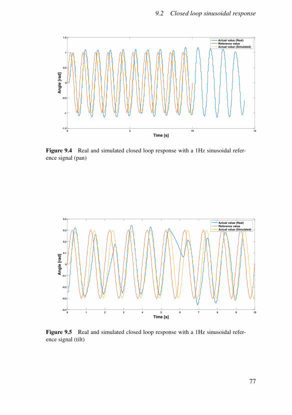
9.2 Closed loop sinusoidal response

0 5 10 15

Time [s]

-1.5

-1

-0.5

0

0.5

1

1.5

An

gle

[ra

d]

Actual value (Real)Reference valueActual value (Simulated)

Figure 9.4 Real and simulated closed loop response with a 1Hz sinusoidal refer-ence signal (pan)

0 1 2 3 4 5 6 7 8 9 10

Time [s]

-0.4

-0.3

-0.2

-0.1

0

0.1

0.2

0.3

0.4

An

gle

[ra

d]

Actual value (Real)Reference valueActual value (Simulated)

Figure 9.5 Real and simulated closed loop response with a 1Hz sinusoidal refer-ence signal (tilt)

77

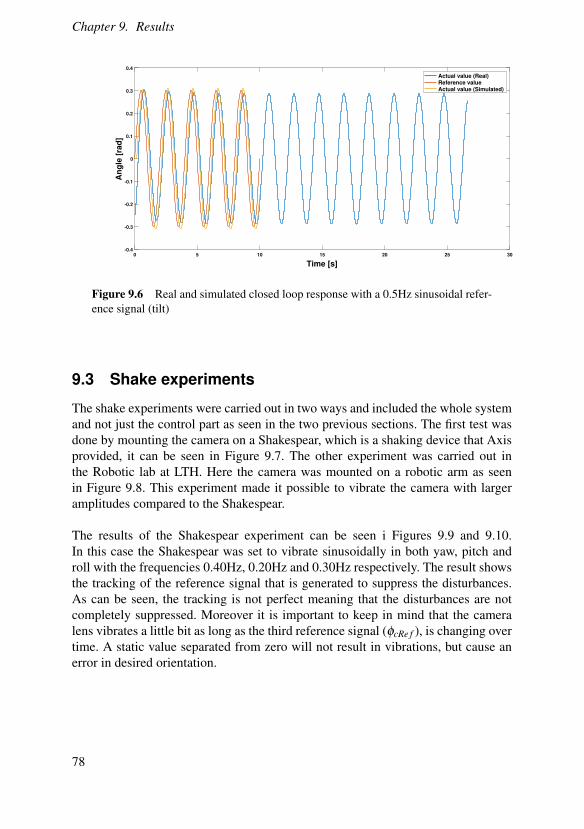
Chapter 9. Results

0 5 10 15 20 25 30

Time [s]

-0.4

-0.3

-0.2

-0.1

0

0.1

0.2

0.3

0.4

An

gle

[ra

d]

Actual value (Real)Reference valueActual value (Simulated)

Figure 9.6 Real and simulated closed loop response with a 0.5Hz sinusoidal refer-ence signal (tilt)

9.3 Shake experiments

The shake experiments were carried out in two ways and included the whole systemand not just the control part as seen in the two previous sections. The first test wasdone by mounting the camera on a Shakespear, which is a shaking device that Axisprovided, it can be seen in Figure 9.7. The other experiment was carried out inthe Robotic lab at LTH. Here the camera was mounted on a robotic arm as seenin Figure 9.8. This experiment made it possible to vibrate the camera with largeramplitudes compared to the Shakespear.

The results of the Shakespear experiment can be seen i Figures 9.9 and 9.10.In this case the Shakespear was set to vibrate sinusoidally in both yaw, pitch androll with the frequencies 0.40Hz, 0.20Hz and 0.30Hz respectively. The result showsthe tracking of the reference signal that is generated to suppress the disturbances.As can be seen, the tracking is not perfect meaning that the disturbances are notcompletely suppressed. Moreover it is important to keep in mind that the cameralens vibrates a little bit as long as the third reference signal (φcRe f ), is changing overtime. A static value separated from zero will not result in vibrations, but cause anerror in desired orientation.

78

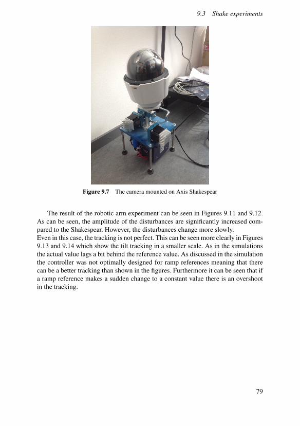
9.3 Shake experiments

Figure 9.7 The camera mounted on Axis Shakespear

The result of the robotic arm experiment can be seen in Figures 9.11 and 9.12.As can be seen, the amplitude of the disturbances are significantly increased com-pared to the Shakespear. However, the disturbances change more slowly.Even in this case, the tracking is not perfect. This can be seen more clearly in Figures9.13 and 9.14 which show the tilt tracking in a smaller scale. As in the simulationsthe actual value lags a bit behind the reference value. As discussed in the simulationthe controller was not optimally designed for ramp references meaning that therecan be a better tracking than shown in the figures. Furthermore it can be seen that ifa ramp reference makes a sudden change to a constant value there is an overshootin the tracking.

79

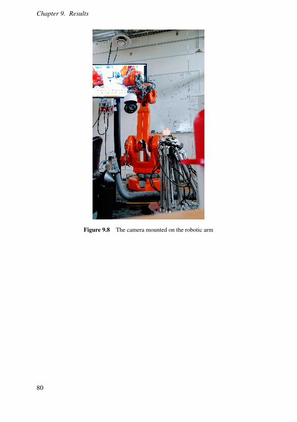
Chapter 9. Results

Figure 9.8 The camera mounted on the robotic arm

80

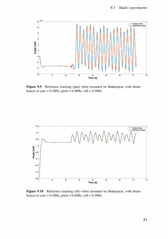
9.3 Shake experiments

0 10 20 30 40 50 60 70 80

Time [s]

-6

-4

-2

0

2

4

6

8

10

12

An

gle

[ra

d]

×10-3

Actual valueReference value

Figure 9.9 Reference tracking (pan) when mounted on Shakespear, with distur-bances in yaw = 0.20Hz, pitch = 0.40Hz, roll = 0.30Hz

0 10 20 30 40 50 60 70 80

Time [s]

-0.25

-0.2

-0.15

-0.1

-0.05

0

0.05

0.1

0.15

An

gle

[ra

d]

Actual valueReference value

Figure 9.10 Reference tracking (tilt) when mounted on Shakespear, with distur-bances in yaw = 0.20Hz, pitch = 0.40Hz, roll = 0.30Hz

81

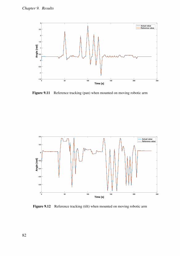
Chapter 9. Results

0 50 100 150 200 250

Time [s]

-1.5

-1

-0.5

0

0.5

1

1.5

2

2.5

3

An

gle

[ra

d]

Actual value

Reference value

Figure 9.11 Reference tracking (pan) when mounted on moving robotic arm

0 50 100 150 200 250

Time [s]

-1

-0.8

-0.6

-0.4

-0.2

0

0.2

0.4

An

gle

[ra

d]

Actual value

Reference value

Figure 9.12 Reference tracking (tilt) when mounted on moving robotic arm

82

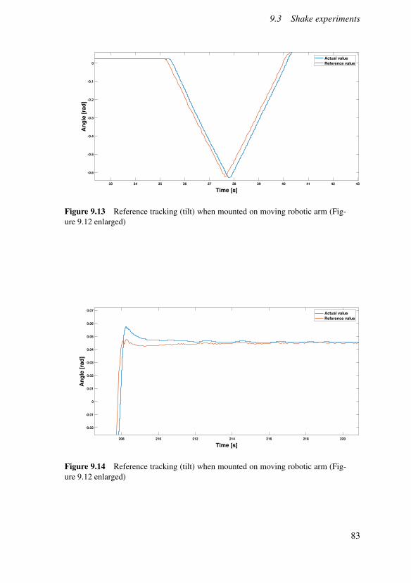
9.3 Shake experiments

33 34 35 36 37 38 39 40 41 42 43

Time [s]

-0.6

-0.5

-0.4

-0.3

-0.2

-0.1

0

An

gle

[ra

d]

Actual value

Reference value

Figure 9.13 Reference tracking (tilt) when mounted on moving robotic arm (Fig-ure 9.12 enlarged)

208 210 212 214 216 218 220

Time [s]

-0.02

-0.01

0

0.01

0.02

0.03

0.04

0.05

0.06

0.07

An

gle

[ra

d]

Actual value

Reference value

Figure 9.14 Reference tracking (tilt) when mounted on moving robotic arm (Fig-ure 9.12 enlarged)

83

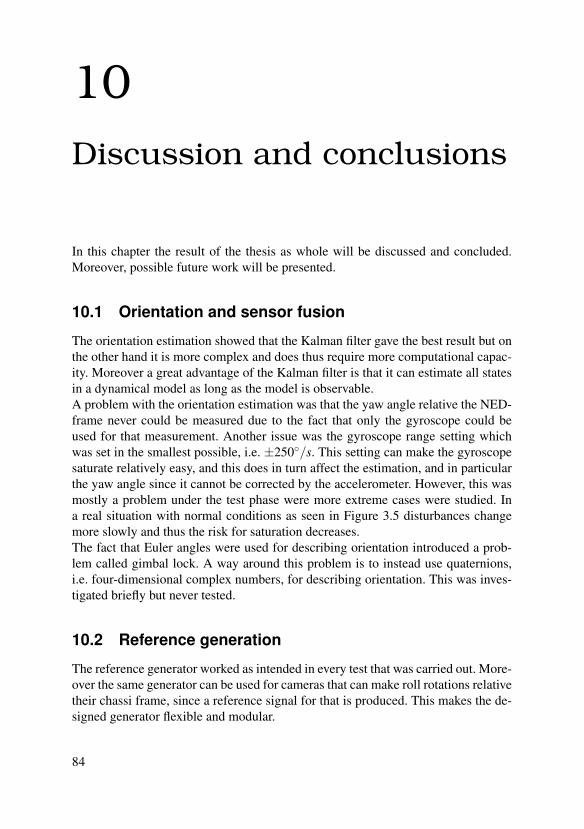
10Discussion and conclusions

In this chapter the result of the thesis as whole will be discussed and concluded.Moreover, possible future work will be presented.

10.1 Orientation and sensor fusion

The orientation estimation showed that the Kalman filter gave the best result but onthe other hand it is more complex and does thus require more computational capac-ity. Moreover a great advantage of the Kalman filter is that it can estimate all statesin a dynamical model as long as the model is observable.A problem with the orientation estimation was that the yaw angle relative the NED-frame never could be measured due to the fact that only the gyroscope could beused for that measurement. Another issue was the gyroscope range setting whichwas set in the smallest possible, i.e. ±250/s. This setting can make the gyroscopesaturate relatively easy, and this does in turn affect the estimation, and in particularthe yaw angle since it cannot be corrected by the accelerometer. However, this wasmostly a problem under the test phase were more extreme cases were studied. Ina real situation with normal conditions as seen in Figure 3.5 disturbances changemore slowly and thus the risk for saturation decreases.The fact that Euler angles were used for describing orientation introduced a prob-lem called gimbal lock. A way around this problem is to instead use quaternions,i.e. four-dimensional complex numbers, for describing orientation. This was inves-tigated briefly but never tested.

10.2 Reference generation

The reference generator worked as intended in every test that was carried out. More-over the same generator can be used for cameras that can make roll rotations relativetheir chassi frame, since a reference signal for that is produced. This makes the de-signed generator flexible and modular.

84

10.3 Modelling

10.3 Modelling

The model obtained from system identification was as mentioned in the final resultsnot good enough for the tilt-system. The best approach for the modelling wouldprobably have been to use the motion profile as described in Chapter 7, but this wasrealized in the end of the thesis.The physical model is more general and would have been used if no internal motioncontroller had been present. A particularly strong property of the gimbal model isthat it describes the cross-coupling between the systems, and this is not taken intoconsideration when using the motion profile.The hybrid stepper motors are as seen in Chapter 6 described by four non-lineardifferential equations. This non-linearty could have been avoided if, for example,brushless DC-motors had been used instead.

10.4 Control and implementation

The control concept has been shown to work, but the controllers can be better tunedor even changed for another controller type. Gain scheduling can, for example, betested in order to handle the tilt nonlinearity. In the beginning of the project Modelpredictive control (MPC) was also considered but was never investigated in depthdue to the model uncertainty.The mid-ranging solution can also be used for future projects since it might bedesired to let the electronic image stabilization work together with the mechanicalimage stabilization.

The code implementation was placed relatively high in the camera code struc-ture. i.e., on the MCPU. If the PID-algorithm had been implemented on the MCUinstead delays could have been decreased. This because orientation estimation andreference generation could have been done parallel to the PID-algorithm.The code that is implemented can also be optimized in order to improve perfor-mance.

85

Chapter 10. Discussion and conclusions

10.5 Future work

In order to improve the product, the code needs to be refined and a separation of thedifferent systems, i.e. making them work independent of each other, would improvethe controllers in particular.

Trying to get the EIS-system, that Axis already have implemented, to collabo-rate with the mechanical image stabilization will improve the stabilization as it thenwill be able to handle disturbances with higher frequency. A mid-ranging solution,as the one described in Chapter 8, could perhaps be used for this purpose.

Another aspect that is more control related is to investigate other controllertypes. As mentioned earlier this can for example be MPC, IMC or gain-scheduledcontrollers.

Lastly, an investigation of the physical model will most certainly improve theproduct since the current model is uncertain. Another advantage with this is that thecontrol system then can be implemented in other cameras, with similar construction,more easily.

10.6 Conclusions

To conclude it can be said that almost all the goals that were stated in the intro-duction were fulfilled. The only goal that was not fulfilled was the requirement of a1Hz closed-loop bandwidth for the tilt-system. However, the result is good enoughto show that mechanical image stabilization is feasible with the Axis camera Q6155-E. The camera was, however, never mounted on a boat but it can be concluded thatthe stabilization will work as long as the disturbances is within the closed-loopbandwidths. Moreover it is not guaranteed that the stabilization will work for othercameras, since the dynamical model that has been used only holds for the currentmotion profile configuration. As always, improvements can be made.

86

Bibliography

Abdo, M., A. R. Vali, A. Toloei, and M. R. Arvan (2013). “Research on the cross-coupling of a two axes gimbal system with dynamic unbalance”. InternationalJournal of Advanced Robotic Systems 10:10, p. 357. DOI: 10.5772/56963.URL: http://dx.doi.org/10.5772/56963.

Acarnely, P. (2002). Stepping Motors: A Guide to Theory and Practice (ControlEngineering) (Control, Robotics and Sensors). Institution of Engineering andTechnology.

Alexandre Karpenko David Jacobs, J. B. (2011). Digital Video Stabilizationand Rolling Shutter Correction using Gyroscopes. Technical Report. Stan-ford University Computer Science. URL: https://graphics.stanford.edu/papers/stabilization/karpenko_gyro.pdf.

Alves Neto, A., D. G. A. Macharet, V. A.-c.C.d. S. Campos, and M. F. M. Campos(2009). “Adaptive complementary filtering algorithm for mobile robot local-ization”. en. Journal of the Brazilian Computer Society 15, pp. 19 –31. ISSN:0104-6500.

Axis (2017). Visited: 2017-03-02. URL: https://www.axis.com.Bilting, U. and J. Skansholm (2011). Vägen till C. Lund, Studentlitteratur, 2011

(Ungern). ISBN: 9789144076065.CHRobotics (2012). Understanding Euler Angles. Tech. rep. Visited:

2017-03-10. URL: http://www.chrobotics.com/docs/AN-1005-UnderstandingEulerAngles.pdf.

Day, M. (2012). “Extracting euler angles from a rotation matrix”. Visited on 2017-05-04. URL: https://d3cw3dd2w32x2b.cloudfront.net/wp-content/uploads/2012/07/euler-angles1.pdf.

Elmenreich, W. (2002). An Introduction to Sensor Fusion. Tech. rep. ResearchReport 47/2001. Institut für Technische Informatik Vienna University of Tech-nology, Austria. URL: https://www.researchgate.net/publication/267771481_An_Introduction_to_Sensor_Fusion.

87

Bibliography

Forsman, K. (2005). Reglerteknik för processindustrin. Lund, Studentlitteratur,2005. ISBN: 9144037899.

Glad, T. and L. Ljung (2003). Reglerteori : flervariabla och olinjära metoder. Lund,Studentlitteratur, 2003. ISBN: 9144030037.

Golik, B. (2006). Development of a Test Method for Image Stabilizing Systems.Matr.-Nr. 11038740, Visited: 2017-03-03. Department of Imaging Sciencesand Media Technology Cologne University of Applied Sciences. URL: https://www.image-engineering.de/content/library/diploma_thesis/borys_golik_image_stabilizers.pdf.

Haschke, R., E. Weitnauer, and H. Ritter (2008). “On-line planning of time-optimal,jerk-limited trajectories”. In: 2008 IEEE/RSJ International Conference on In-telligent Robots and Systems, pp. 3248–3253. DOI: 10.1109/IROS.2008.4650924.

Higgins, W. T. (1975). “A comparison of complementary and kalman filtering”.IEEE Transactions on Aerospace and Electronic Systems AES-11:3, pp. 321–325. ISSN: 0018-9251. DOI: 10.1109/TAES.1975.308081.

Kepinski, R., J. Awrejcewicz, and D. Lewandowski (2015). “Dynamical simulationof a nonlinear stepper motor system”. International Journal of Dynamics andControl 3:1, pp. 31–35. ISSN: 2195-2698. DOI: 10.1007/s40435-014-0093-6. URL: https://doi.org/10.1007/s40435-014-0093-6.

Kröger, T. and F. M. Wahl (2010). “Online trajectory generation: basic concepts forinstantaneous reactions to unforeseen events”. IEEE Transactions on Robotics26:1, pp. 94–111. ISSN: 1552-3098. DOI: 10.1109/TRO.2009.2035744.

Kröger, T., A. Tomiczek, and F. M. Wahl (2006). “Towards on-line trajectory com-putation”. In: 2006 IEEE/RSJ International Conference on Intelligent Robotsand Systems, pp. 736–741. DOI: 10.1109/IROS.2006.282622.

Lambrechts, P., M. Boerlage, and M. Steinbuch (2005). “Trajectory planning andfeedforward design for electromechanical motion systems.” Control Engineer-ing Practice 13, pp. 145 –157. ISSN: 0967-0661.

Lewin, C. (2007). Mathematics of Motion Control Profiles. Technical Report. 2017-05-08. Performance Motion Devices. URL: https://performance-motion-devices.s3.amazonaws.com/pdfs/White%20Papers/Mathematics_of_Motion_Control_Profiles.pdf.

Linderoth, M. (2013). On Robotic Work-Space Sensing and Control. PhD thesisTFRT-1098. Department of Automatic Control, Lund University, Sweden.

Ljung, L. (2007). System Identification. Tech. rep. 2809. Linköping University, Au-tomatic Control, p. 65.

Ljung, L. and T. Glad (2004). Modellbygge och simulering. Lund, Studentlitteratur,2004. ISBN: 9144024436.

88

Bibliography

Pedeley, M. (2013). Tilt sensing using a three-axis accelerometer. Tech. rep. Visited:2017-03-27. URL: https://cache.freescale.com/files/sensors/doc/app_note/AN3461.pdf.

Pycke, T. (2006). Kalman filtering of imu data. Visited: 2017-04-14. URL: http://tom.pycke.be/mav/71/kalman-filtering-of-imu-data.

Reflexxes (2017). Visited: 2017-03-06. URL: http://www.reflexxes.ws/reflexxes-motion-libraries-details.html.

ROHM-Semiconductor (2017). Optical Image Stabilization (OIS). Technical Re-port. Visited: 2017-03-15. ROHM Semiconductor. URL: http://www.rohm.com/documents/11308/12928/OIS-white-paper.pdf.

Sloth Lauszus, K. (2012). “A practical approach to Kalman filter and how toimplement it”. TKJ Electronics. Visited: 2017-04-26. URL: http://blog.tkjelectronics.dk/2012/09/a-practical-approach-to-kalman-filter-and-how-to-implement-it/.

Thomas, B. (2008). Modern reglerteknik. Stockholm, Liber, 2008 (Slovenien).ISBN: 9147093234.

Trinamic (2017). Visited: 2017-04-08. URL: https://www.trinamic.com/.Wittenmark, B., K.-E. Årzén, and K. J. Åström (2014). Computer Control: An

Overview. Technical Report. Department of Automatic Control, Lund Uni-versity, Sweden. URL: https://www.ifac-control.org/publications/list-of-professional-briefs/pb_wittenmark_etal_final.pdf/view?searchterm=computer+control%3A+An+overview.

Zhi, R. (2016). A Drift Eliminated & Position Estimation Algorithm In 3D. Master’sthesis 450. University of Vermont, USA. URL: http://scholarworks.uvm.edu/graddis/450/.

Årzén, K.-E. (2014). Real-time control systems. Lund University, Department ofAutomatic Control.

Åström, K. J. and R. M. Murray (2008). Feedback systems : an introduction forscientists and engineers. Princeton, N.J. : Princeton University Press, cop. 2008.ISBN: 9780691135762.

89

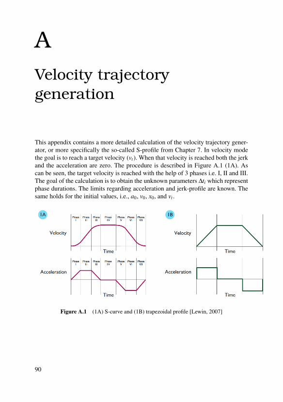
AVelocity trajectorygeneration

This appendix contains a more detailed calculation of the velocity trajectory gener-ator, or more specifically the so-called S-profile from Chapter 7. In velocity modethe goal is to reach a target velocity (vt ). When that velocity is reached both the jerkand the acceleration are zero. The procedure is described in Figure A.1 (1A). Ascan be seen, the target velocity is reached with the help of 3 phases i.e. I, II and III.The goal of the calculation is to obtain the unknown parameters ∆ti which representphase durations. The limits regarding acceleration and jerk-profile are known. Thesame holds for the initial values, i.e., a0, v0, x0, and vt .

Figure A.1 (1A) S-curve and (1B) trapezoidal profile [Lewin, 2007]

90

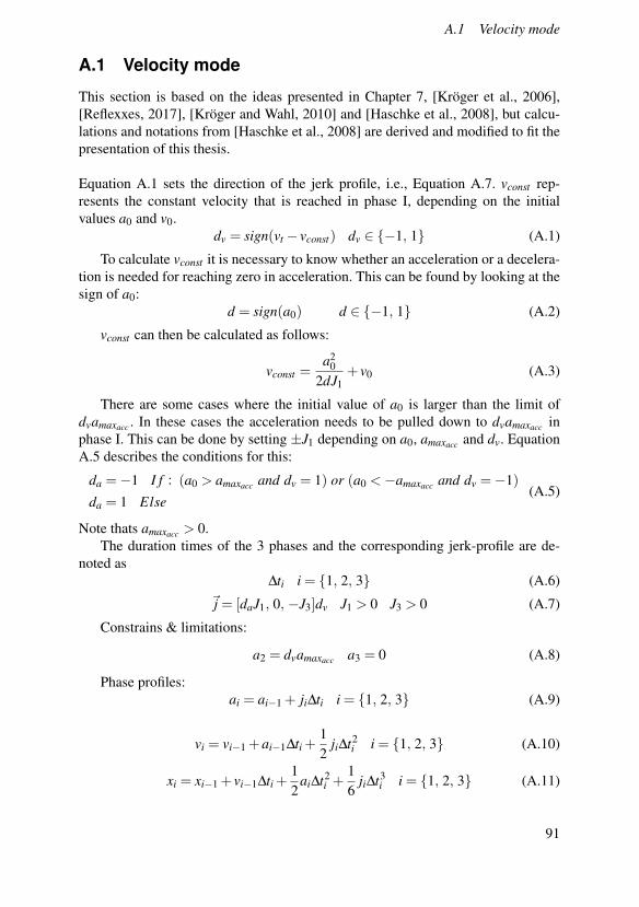
A.1 Velocity mode

A.1 Velocity mode

This section is based on the ideas presented in Chapter 7, [Kröger et al., 2006],[Reflexxes, 2017], [Kröger and Wahl, 2010] and [Haschke et al., 2008], but calcu-lations and notations from [Haschke et al., 2008] are derived and modified to fit thepresentation of this thesis.

Equation A.1 sets the direction of the jerk profile, i.e., Equation A.7. vconst rep-resents the constant velocity that is reached in phase I, depending on the initialvalues a0 and v0.

dv = sign(vt − vconst) dv ∈ −1, 1 (A.1)

To calculate vconst it is necessary to know whether an acceleration or a decelera-tion is needed for reaching zero in acceleration. This can be found by looking at thesign of a0:

d = sign(a0) d ∈ −1, 1 (A.2)

vconst can then be calculated as follows:

vconst =a2

02dJ1

+ v0 (A.3)

There are some cases where the initial value of a0 is larger than the limit ofdvamaxacc . In these cases the acceleration needs to be pulled down to dvamaxacc inphase I. This can be done by setting ±J1 depending on a0, amaxacc and dv. EquationA.5 describes the conditions for this:

da =−1 I f : (a0 > amaxacc and dv = 1) or (a0 <−amaxacc and dv =−1)da = 1 Else

(A.5)

Note thats amaxacc > 0.The duration times of the 3 phases and the corresponding jerk-profile are de-

noted as∆ti i = 1, 2, 3 (A.6)

~j = [daJ1, 0, −J3]dv J1 > 0 J3 > 0 (A.7)

Constrains & limitations:

a2 = dvamaxacc a3 = 0 (A.8)

Phase profiles:ai = ai−1 + ji∆ti i = 1, 2, 3 (A.9)

vi = vi−1 +ai−1∆ti +12

ji∆t2i i = 1, 2, 3 (A.10)

xi = xi−1 + vi−1∆ti +12

ai∆t2i +

16

ji∆t3i i = 1, 2, 3 (A.11)

91

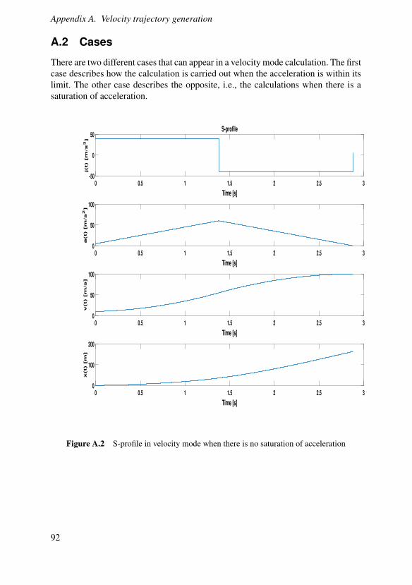
Appendix A. Velocity trajectory generation

A.2 Cases

There are two different cases that can appear in a velocity mode calculation. The firstcase describes how the calculation is carried out when the acceleration is within itslimit. The other case describes the opposite, i.e., the calculations when there is asaturation of acceleration.

0 0.5 1 1.5 2 2.5 3

Time [s]

-50

0

50

j(t) [m

/s

3]

S-profile

0 0.5 1 1.5 2 2.5 3

Time [s]

0

50

100

a(t) [m

/s

2]

0 0.5 1 1.5 2 2.5 3

Time [s]

0

50

100

v(t) [m

/s

]

0 0.5 1 1.5 2 2.5 3

Time [s]

0

100

200

x(t) [m

]

Figure A.2 S-profile in velocity mode when there is no saturation of acceleration

92

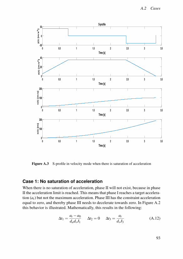
A.2 Cases

0 0.5 1 1.5 2 2.5 3 3.5

Time [s]

-50

0

50

j(t) [m

/s

3]

S-profile

0 0.5 1 1.5 2 2.5 3 3.5

Time [s]

0

20

40

a(t) [m

/s

2]

0 0.5 1 1.5 2 2.5 3 3.5

Time [s]

0

100

200

v(t) [m

/s

]

0 0.5 1 1.5 2 2.5 3 3.5

Time [s]

0

100

200

x(t) [m

]

Figure A.3 S-profile in velocity mode when there is saturation of acceleration

Case 1: No saturation of accelerationWhen there is no saturation of acceleration, phase II will not exist, because in phaseII the acceleration limit is reached. This means that phase I reaches a target accelera-tion (at ) but not the maximum acceleration. Phase III has the constraint accelerationequal to zero, and thereby phase III needs to decelerate towards zero. In Figure A.2this behavior is illustrated. Mathematically, this results in the following:

∆t1 =at −a0

dadvJ1∆t2 = 0 ∆t3 =

at

dvJ3(A.12)

93

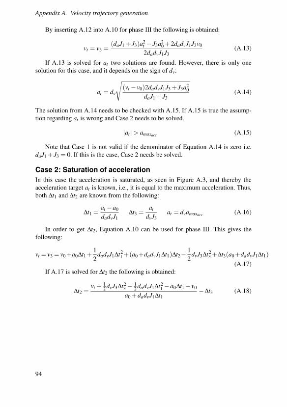
Appendix A. Velocity trajectory generation

By inserting A.12 into A.10 for phase III the following is obtained:

vt = v3 =(daJ1 + J3)a2

t − J3a20 +2dadvJ1J3v0

2dadvJ1J3(A.13)

If A.13 is solved for at two solutions are found. However, there is only onesolution for this case, and it depends on the sign of dv:

at = dv

√(vt − v0)2dadvJ1J3 + J3a2

0daJ1 + J3

(A.14)

The solution from A.14 needs to be checked with A.15. If A.15 is true the assump-tion regarding at is wrong and Case 2 needs to be solved.

|at |> amaxacc (A.15)

Note that Case 1 is not valid if the denominator of Equation A.14 is zero i.e.daJ1 + J3 = 0. If this is the case, Case 2 needs be solved.

Case 2: Saturation of accelerationIn this case the acceleration is saturated, as seen in Figure A.3, and thereby theacceleration target at is known, i.e., it is equal to the maximum acceleration. Thus,both ∆t1 and ∆t2 are known from the following:

∆t1 =at −a0

dadvJ1∆t3 =

at

dvJ3at = dvamaxacc (A.16)

In order to get ∆t2, Equation A.10 can be used for phase III. This gives thefollowing:

vt = v3 = v0+a0∆t1+12

dadvJ1∆t21 +(a0+dadvJ1∆t1)∆t2−

12

dvJ3∆t23 +∆t3(a0+dadvJ1∆t1)

(A.17)If A.17 is solved for ∆t2 the following is obtained:

∆t2 =vt +

12 dvJ3∆t2

3 −12 dadvJ1∆t2

1 −a0∆t1− v0

a0 +dadvJ1∆t1−∆t3 (A.18)

94

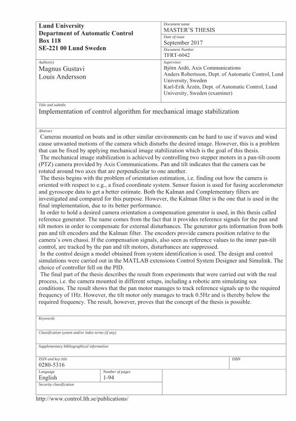
Document name

Date of issue

Document Number

Author(s) Supervisor

Title and subtitle

Abstract

Keywords

Classification system and/or index terms (if any)

Supplementary bibliographical information

ISSN and key title ISBN

Language Number of pages

Security classification