IMPLEMENTATION OF FIBER ELEMENT

MODEL FOR NON-LINEAR ANALYSIS

Shemin T John

DEPARTMENT OF CIVIL ENGINEERING

NATIONAL INSTITUTE OF TECHNOLOGY

ROURKELA 769008

May 2015

Implementation of Fiber element model for

Non-linear analysis

A thesis

Submitted by

SHEMIN T JOHN (213CE2064)

In partial fulfilment of the requirements for

the award of the degree

of

MASTER OF TECHNOLOGY

In

STRUCTURAL ENGINEERING

Under the Guidance of

Dr. ROBIN DAVIS P

DEPARTMENT OF CIVIL ENGINEERING

NATIONAL INSTITUTE OF TECHNOLOGY, ROURKELA 769008

May 2015

NATIONAL INSTITUTE OF TECHNOLOGY

ROURKELA- 769008, ORISSA

INDIA

CERTIFICATE

This is to certify that the thesis entitled “Implementation of Fiber element model for Non-linear

analysis” submitted by Shemin T John in partial fulfilment of the requirement for the award of

Master of Technology degree in Civil Engineering with specialization in Structural Engineering

to the National Institute of Technology, Rourkela is an authentic record of research work carried

out by her under my supervision. The contents of this thesis, in full or in parts, have not been

submitted to any other Institute or University for the award of any degree or diploma.

Project Guide

Dr. ROBIN DAVIS P

Assistant Professor

Department of Civil Engineering

ACKNOWLEDGEMENTS

First and foremost, praises and thanks to the God, the Almighty, for his showers of blessings

throughout my work to complete the research successfully.

I would like to express my sincere gratitude to my guide Dr. ROBIN DAVIS P for

enlightening me with the first glance of research, and for his patience, motivation, enthusiasm,

and immense knowledge. His guidance helped me in all the time of research and writing of this

thesis. I could not have imagined having a better advisor and mentor for my project work. It was

a great privilege and honour to work and study under his guidance. I am extremely grateful for what

he has offered me. I am extending my heartfelt thanks to his wife, family for their acceptance and

patience during the discussion I had with him on research work and thesis preparation.

Besides my advisor I extend my sincere thanks to Dr. Pradip.Sarkar, Dr. Manoranjan

Barik, and all faculties in Structural Engineering Department, NIT Rourkela for their

timely co-operations during the project work.

It gives me great pleasure to acknowledge the support and help of Kananika Nayak, and Aparna K Sathyan for their help throughout my research work. Last but not the least; I would like to thank my family, for supporting me spiritually throughout

my life and for their unconditional love, moral support and encouragement. So many people have contributed to my research work, and it is with great pleasure to take the

opportunity to thank them. I apologize, if I have forgotten anyone.

SHEMIN T JOHN

Table of Contents

LIST OF FIGURES .................................................................................................................... 1

LIST OF TABLES ................................................................................................................. 2

LIST OF SYMBOLS .................................................................................................................. 3

ABSTRACT .................................................................................................................................

1. INTRODUCTION................................................................................................................... 1

1.1 GENERAL ........................................................................................................................ 2

1.2 NONLINEAR MODELLING OF RC ELEMENTS .......................................................... 2

1.2.1 DISTRIBUTED PLASTICITY AND LUMPED PLASTICITY ........................... 2

1.3 OBJECTIVE OF THE PRESENT STUDY ........................................................................ 3

1.4 METHODOLOGY ............................................................................................................ 4

1.5 SCOPE OF WORK ............................................................................................................ 4

1.6 ORGANIZATION OF THESIS ......................................................................................... 4

2. LITRETURE RIVIEW ............................................................................................................ 6

2.1 GENERAL ........................................................................................................................ 7

2.2 DISTRIBUTED INELASTICITY MODELS .................................................................... 7

2.2.1 DISPLACEMENT BASED STIFFNESS METHOD ................................ 7

2.2.2 FORCE BASED FLEXIBILITYL METHOD ........................................... 9

2.3 NUMERICAL INTEGRATION ..................................................................................... 10

2.4 SOLUTION STRATEGIES FOR NONLINEAR ANALYSIS ........................................ 11

2.4.1 PATH FOLLOWING TECHNIQUES ............................................................... 11

2.4.1.1 LOAD CONTROL METHOD ................................................................ 11

2.4.1.1 DISPLACEMENT CONTROL METHOD ............................................. 11

2.5 ITERATIVE TECHNIQUES FOR NON-LINEAR ANALYSIS...................................... 15

2.5.1 NEWTON RAPHSON METHOD ..................................................................... 15

2.6 CONFINEMENT MODELS FOR CONCRETE ............................................................. 16

2.6.1 MANDER et al. (1988) MODEL ............................................................ 16

2.6.2 MODIFIED KENT AND PARK MODEL (1982) .................................. 17

2.6.3 IS 456 (2000) MODEL ........................................................................... 19

2.6.4 NON LINEAR STEEL MODEL ........................................................... 20

2.7 MONTE CARLO SIMULATION ................................................................................... 20

2.8 SUMMARY .................................................................................................................... 22

3.ELEMENT FORMULATIONS ............................................................................................. 23

3.1 GENERAL ................................................................................................................. 24

3.2 DISPLACEMENT BASED-STIFFNESS METHOD .................................................. 24

3.3 FLEXIBILITY BASED-FORCE METHOD .............................................................. 26

3.4 SUMMARY ............................................................................................................... 28

4 IMPLEMENTATION OF FIBER ELEMENT FOR PROBABILISTIC ANALYSIS............. 29

4.1. GENERAL ................................................................................................................. 30

4.2. METHODOLOGY ..................................................................................................... 30

4.3 PROCEDURE FOR STIFFNESS AND FLEXIBILITY BASED METHOD ............... 31

4.4 COMPARISON OF LINEAR ANALYSIS USING DB AND FB FORMULATION ...... 33

4.4.1 ELASTIC COLUMN WITH AXIAL FORCE....................................................... 33

4.5 CONVERGENCE STUDY - DIRECT INTERATION .................................................... 35

4.6 CONVERGENCE STUDY - NUMERICAL INTEGRATION ........................................ 38

4.7 COMPARISON BETWEEN DIRECT AND NUMERICAL INTEGRATION ................ 39

4.8CONFINEMENT MODELS IN NON-LINEAR RESPONSE .......................................... 40

4.9 RC COLUMN WITH AXIAL COMPRESSION ............................................................. 41

4.10 PROBABILISTIC STUDIES ........................................................................................ 46

4.11 SUMMARY ................................................................................................................. 55

5.SUMMARY AND CONCLUSIONS ..................................................................................... 56

5.1 GENERAL ................................................................................................................. 57

5.2 CONCLUSIONS ........................................................................................................ 57

5.3 LIMITATION AND FUTURE SCOPE OF WORK ................................................... 58

REFERENCES

LIST OF FIGURES

Title Page No

Fig.1.1 Zero length spring used in lumped plasticity model ........................................................ 2

Fig.1.2 Fiber section discretization and sections ......................................................................... 3

Fig.2.1 Locations and Weights of Gauss Lobatto quadrature rules ............................................ 11

Fig.2.2 Load control and Displacement control method (reference) ........................................... 12

Fig.2.3 Flow chart for Displacement control method ................................................................ 14

Fig. 2.4: Newton Raphson iterative scheme .............................................................................. 15

Fig. 2.5: Mander et al 1988 model ............................................................................................ 17

Fig. 2.6: Modified Kent and Park model (1982)......................................................................... 18

Fig. 2.7: IS 456 model (2000) .................................................................................................... 19

Fig. 2.8: Steel constitutive model (Lee and Mosalam, 2004). ..................................................... 20

Fig. 3.1: Element force and deformations ................................................................................. 25

Fig. 4.1: Flow chart showing the present study ......................................................................... 31

Fig. 4.2a: Flow chart of state determination of Stiffness based method ..................................... 32

Fig. 4.2b: Flow chart of state determination of Flexibility based method. .................................. 33

Fig. 4.3: Homogenous column subjected to axial compression ................................................. 34

Fig. 4.4: Force Displacement response for Elastic Column using DBM and FBM ..................... 35

Fig. 4.5: Cantilever beam with point load at the end ................................................................. 36

Fig. 4.6: Deflection comparison for direct integration ............................................................... 37

Fig. 4.7: Percentage error comparison for direct integration ...................................................... 37

Fig. 4.8: Deflection comparison for Numerical Integration. ....................................................... 39

Fig 4.9: Error comparison for Numerical Integration ................................................................ 39

Fig. 4.10: Number of fiber comparison for both integrations. ..................................................... 40

Fig. 4.11: Execution time comparison for both integrations ...................................................... 40

Fig. 4.12: RC Column subjected to different stress strain models .............................................. 43

Fig 4.13: RC column with confined and unconfined sections using Mander et. al, (1988) ......... 44

Fig. 4.14: RC column, entire section as unconfined concrete as per Mander et al. (1988)........... 44

Fig. 4.15: RC column with concrete stress -strain using IS 456(2000) model ............................ 45

Fig. 4.16: Nonlinear Response of RC column with Kent Park (1971) model ............................. 45

Fig. 4.17: Comparison of force versus deformation of RC column with

axial loading using different confinement models for concrete .................................. 46

Fig 4.18: Flow chart of the probabilistic fiber element approach ............................................... 48

Fig 4.19: Probability distribution of Compressive strength of concrete ..................................... 49

Fig. 4.20 Probability distribution of yield strength of steel ........................................................ 50

Fig 4.21: Probability distribution of width of beam ................................................................... 50

Fig. 4.22 Probability distribution of depth of beam ................................................................... 50

Fig 4.23 Probability distribution of length of beam ................................................................... 51

Fig. 4.24 Probability distribution of Initial tangent modulus of concrete ................................... 51

Fig 4.25: Probability distribution of Compressive strength of concrete ..................................... 52

Fig. 4.26 Probability distribution of initial tangent modulus of concrete ................................... 52

Fig. 4.27 Histogram for peak axial strength using IS 456 (2000) model .................................... 53

Fig. 4.28 Histogram for peak axial strength for Modified Kent and Park (1982) ....................... 53

Fig. 4.29: Coefficient of Variation for all the parameters with different models ......................... 54

LIST OF TABLES

Title Page No

Table.2.1 Locations and of the associated weights for Gauss Lobatto integration rule ............... 10

Table.4.1 Parameters for number of fiber elements ................................................................... 34

Table.4.2 Convergence study - Direct integration ..................................................................... 36

Table 4.3:Numerical integration: Fiber cross sections-Deflections and errors ............................ 38

Table 4.4: Parameters and distributions used for generation of random variables ....................... 49

LIST OF SYMBOLS

fc Compressive Strength of Concrete

fy Yield Strength of Steel

Ec Young’s Modulus of Concrete

Es Elastic Modulus of steel

ϵcc Strain corresponding to Compressive strength of Concrete

fco Compressive strength of Unconfined Concrete

ϵco Strain corresponding to Unconfined Compressive strength

ϵcu Ultimate strain of Confined Concrete

ABBREVIATIONS

K Strength Enhancement factor

RC Reinforced Concrete

IS Indian Standard

DBM Displacement Based Method

FBM Force Based Method

MCS Monte Carlo Simulation

ABSTRACT

Keywords: Fiber element, Distributed Inelasticity, Numerical Integration, MCS, Confinement

models for concrete

RC frames undergo inelastic deformations in the event of an extreme earthquake. Nonlinear

modelling of the concrete sections is very much necessary for the simulation of realistic

behaviour of RC frames in earthquake loading. Concentrated/lumped plasticity and distributed

plasticity are the two different approaches for nonlinear modelling of RC elements available in

literature. The main objective of the present study is to implement a displacement based fiber

element (stiffness) for nonlinear analysis of RC Sections. The present study focused on the

element formulation of both stiffness and flexibility based fiber models, direct integration and

numerical integration and incorporation of popular confinement models for stress-strain

relationship for concrete. The present study is extended to a probabilistic analysis using the

implemented model. It is found that fiber elements are appropriate tool for incorporating

nonlinearity in the RC sections.

1 | P a g e

1 INTRODUCTION

2 | P a g e

CHAPTER 1

INTRODUCTION

1.1 GENERAL

RC frames behave inelastically under earthquake loading. Simulation of behaviour of RC frame

in such earthquake loading requires nonlinear modelling and analysis techniques. There two

different types of approaches for nonlinear modelling of RC elements, namely concentrated or

lumped plasticity approach and distributed plasticity approach. The motivation of the present

study is to simulate the nonlinear behaviour of RC sections using a fiber element model.

1.2 NONLINEAR MODELLING OF RC ELEMENTS

Material nonlinearity in a frame elements are primarily divided into two categories;

1.2.1 Distributed plasticity and Lumped plasticity

In the lumped plasticity model, elements consists of two zero-length nonlinear rotational spring

elements with an elastic element between them as shown in the Fig. 1.1 The spring element

accounts for nonlinear behaviour of a structure by having nonlinear moment-rotation

relationships. The lumped plasticity model is popular since the computational cost of the analysis

is high, e.g., in the case of nonlinear time-history analysis of a large structure.

Fig 1.1: Zero length spring used in lumped plasticity model

3 | P a g e

The distributed plasticity model is used for more accurate estimation of the structural response.

The distributed plasticity model is employed for the nonlinear frame element with the fiber

section discretization. The distributed inelasticity members are modelled with the fiber approach,

which consists of discretizing into integration sections and into several material fibers as shown

in Fig. 1.2. The two main formulations are the displacement-based (DB) stiffness method and the

force-based (FB) flexibility method. The DB formulation uses displacement shape functions,

while the FB formulation uses internal force shape functions.

Fig 1.2: Fiber section discretization and sections

1.3 OBJECTIVES OF THE STUDY

Based on the preceding discussions, the main objectives of the current study has been quoted as

follows

i. To implement the displacement based (stiffness) fiber element model for nonlinear

analysis of RC Columns.

ii. To study the response of RC sections using various confinement models of concrete.

4 | P a g e

iii. To conduct probabilistic analysis of RC column considering uncertainties in the geometry

and material properties.

1.4 METHODOLOGY

i. Conduct a literature review on various fiber element models to use in RC sections for

non-linear static analysis.

ii. Identify a simple and easy to implement fiber element models

iii. Implement the fiber element model in MATLAB 2012b.

iv. Perform static non-linear analysis of RC section

v. Consider uncertainty of various random variables involved

vi. Conduct a probabilistic analysis to arrive at the uncertainty in the responses such as base

shear and yield displacement. Analyse the results and arrive at conclusions.

1.5 SCOPE OF WORK

i. The present study is limited to only axial loading of RC sections.

ii. Only distributed plasticity formulations are considered for this study.

iii. Only material nonlinearity is considered in this study

1.6 ORGANISATION OF THE THESIS

Following this introductory chapter, the organisation of further Chapters is done as explained

below.

i. A review of literature conducted on Element formulations of fiber element modelling,

nonlinear solution and iterative strategies constitutive models for steel and concrete, and

Monte Carlo simulation in Chapter 2.

5 | P a g e

ii. Element formulations of stiffness and flexibility fiber element model for the RC

sections is explained in Chapter 3.

iii. Linear and Nonlinear analysis of RC sections using fiber element modelling and

probabilistic studies such as Monte carlo simulations are explained in Chapter 4

iv. Finally in Chapter 5, discussion of results, limitations of the work and future scope of

this study is dealt with.

6 | P a g e

2 REVIEW OF LITERATURE

7 | P a g e

CHAPTER-2

LITERATURE REVIEW

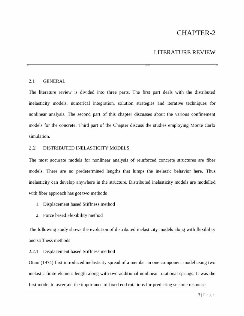
2.1 GENERAL

The literature review is divided into three parts. The first part deals with the distributed

inelasticity models, numerical integration, solution strategies and iterative techniques for

nonlinear analysis. The second part of this chapter discusses about the various confinement

models for the concrete. Third part of the Chapter discuss the studies employing Monte Carlo

simulation.

2.2 DISTRIBUTED INELASTICITY MODELS

The most accurate models for nonlinear analysis of reinforced concrete structures are fiber

models. There are no predetermined lengths that lumps the inelastic behavior here. Thus

inelasticity can develop anywhere in the structure. Distributed inelasticity models are modelled

with fiber approach has got two methods

1. Displacement based Stiffness method

2. Force based Flexibility method

The following study shows the evolution of distributed inelasticity models along with flexibility

and stiffness methods

2.2.1 Displacement based Stiffness method

Otani (1974) first introduced inelasticity spread of a member in one component model using two

inelastic finite element length along with two additional nonlinear rotational springs. It was the

first model to ascertain the importance of fixed end rotations for predicting seismic response.

8 | P a g e

Soleimani et al. (1979) considered a model with gradual spread of inelasticity along the member

It consist of elastic and inelastic zones. The inelastic zones spreads from beam-column interface

controlled by moment curvature relationship at member end section. Point hinges were also

considered for fixed end rotations at beam column interface.

The proposal by Soleimani et al. (1979) was further extended by Filippou and Issa (1988) in a

completely refined way. The member was subdivided into sub elements each accounting elastic

behavior, inelastic behavior due to bending and fixed end rotations at beam column interface.

Flexibility matrix and member end rotations are summed up from each sub element as they are

all associated in series. The point hinge idealization was used in these models are based on

bilinear moment rotation relationship with constant post yielding stiffness. This model was

further improved by Filippou et al (1992) to include another sub element with shear distortions

in inelastic zones. Constant axial force-bending moment interaction was included in the basic

curve of the model.

Takanayagi and schnobrich (1979) have proposed another type of member model dividing

elements into short sub elements (finite element springs) along the member with nonlinear

moment rotation relationships. Axial force-bending moment interaction was included by limit

surface for each spring. This model also encountered problem of unbalanced force in internal

members which often resulted in numerical instability.

This model along with (Hellesland and Scordelis, 1981, Mari and Scordelis, 1984) were based on

classical stiffness method using cubic hermitian polynomials to approximate displacements along

the member. In these types, it encompasses 6 degree of freedom for the 3D elements.

In our present study element formulation presented by Lee and Mosalam (2004) is implemented

which uses displacement interpolation functions from classical stiffness methods. The element

9 | P a g e

stiffness matrix and nodal equivalent forces are obtained by integration of section stiffness and

force distributions. The element formulation is straight forward and easy to implement.

2.2.1 Force based Flexibility method

Menegotto and Pinto (1977) proposed improved representation of internal deformations by

combined approximation for both section deformation and flexibilities. Mahasuverachai (1982)

proposed improvement of displacement interpolation functions. He introduced variable

interpolation functions for piping and tubular structures.

Kaba and Mahin (1984) adapted this to RCC structures along with section layer discretization.

Typically these functions were derived from from force interpolation polynomials. A mixed

approach was used when both deformation and force interpolation functions are used. The model

has inconsistencies led to numerical problems. State determination were such that equilibrium

between applied and resisting section forces were not satisfied. The proposal was further

improved by Zeris et al. (1986) and Kaba and Mahin (1988) improving element state

determination.

The formulation of nonlinear flexibility based frame element cast into a unified and general

theory by Taucer et al. (1991), Spacone et al. (1992) and Spacone (1994) derived from mixed

finite element works of Zienkiewicks and Taylor (1989). Element state determination inserted

classical stiffness based finite element which appear rather straightforward. The formulation was

capable to carry moment curvature relationship or stress strain relationship at the fiber level. It

requires a few control sections along the member. The force interpolation functions were used as

they are exact regardless to the damaged state of the member. Element flexibility matrix were

obtained by integration of flexibility distributions at control sections and an internal iterative

scheme was proposed to find element resisting force for imposed displacements.

10 | P a g e

2.3 NUMERICAL INTEGRATION

Stiffness and Flexibility based formulations requires integration along the length of member.

Conventional direct integrations are computationally not effective. These integrals can be

evaluated by numerical quadrature. In our present study, we use gauss lobatto integration.

Location points xi and weights wi for i = 1,...,n. The domain of integration for such a rule is

conventionally taken as [−1, 1], so the rule can be stated as:

(2.1)

The Gauss-Lobatto rule with ‘n’ Integration points allows the exact integration of polynomials of

degree up to 2n-3. The locations and the associated weights for this integration rule is shown in

the Table 2.1. The points, xi is the locations and wi are the weights.

Table 2.1 Locations and the associated weights for Gauss Lobatto integration rule

Number of points Points,XIP Weights,W

-1.000 0.333

0.000 1.333

1.000 0.333

-1.000 0.167

-0.447 0.833

0.447 0.833

1.000 0.167

-1.000 0.100

-0.655 0.544

0.000 0.711

0.655 0.544

1.000 0.100

3

4

5

11 | P a g e

Fig 2.1: Locations and Weights of Gauss Lobatto quadrature rules

2.4 SOLUTION STRATEGIES FOR NONLINEAR ANALYSIS

2.4.1 Path Following Techniques

The objective of this techniques are to draw the equilibrium path of a nonlinear problem in the

framework of a force-displacement relation. There are many techniques available and a Load

control and Displacement control method is used in the present study.

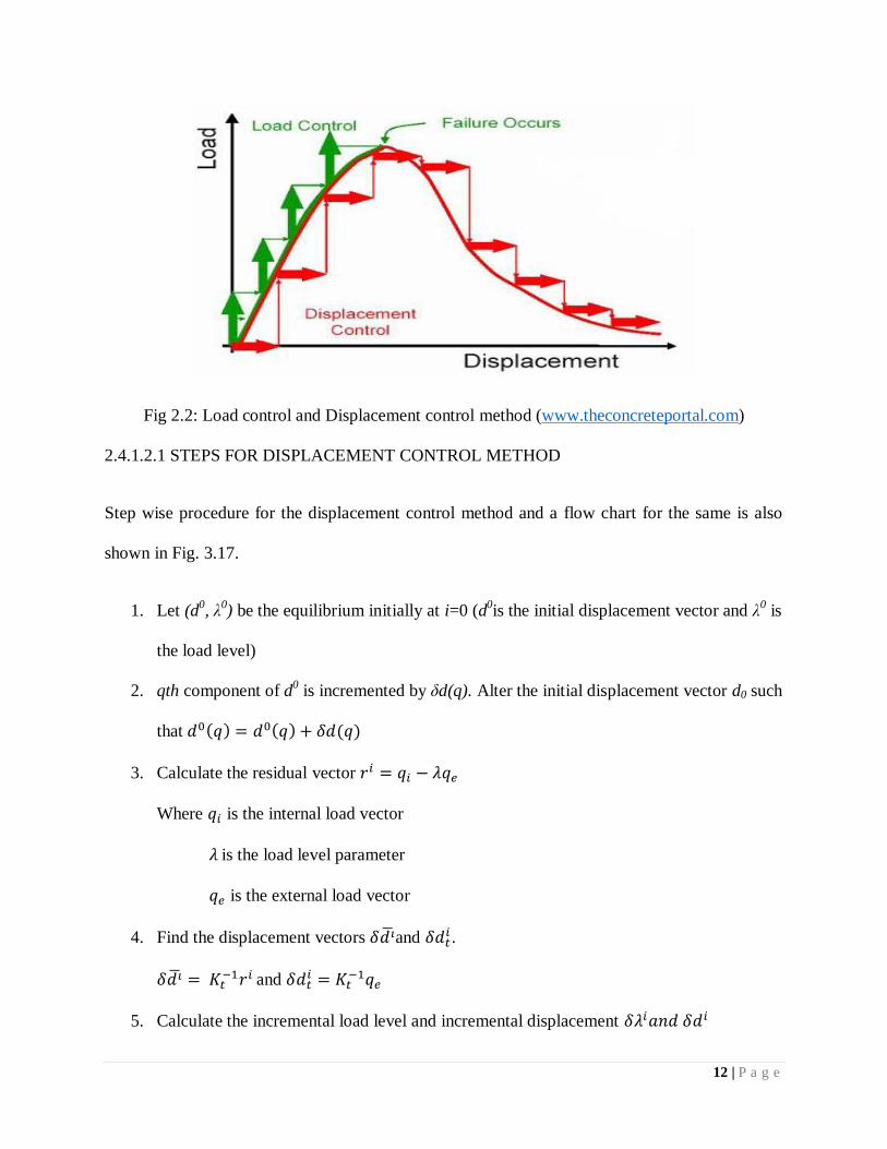
2.4.1.1 Load Control

The total load is divided into small load increments. Displacement is calculated for each load

level. This method gives equilibrium path up to failure point only as shown in the Fig.2.2.This

method is not suitable at post critical yield regions and usually results in instability.

2.4.1.2 Displacement control

Displacement control method gives a good solution for nonlinear problems because it presents a

great stability at the critical points.

12 | P a g e

Fig 2.2: Load control and Displacement control method (www.theconcreteportal.com)

2.4.1.2.1 STEPS FOR DISPLACEMENT CONTROL METHOD

Step wise procedure for the displacement control method and a flow chart for the same is also

shown in Fig. 3.17.

1. Let (d0, λ

0) be the equilibrium initially at i=0 (d

0is the initial displacement vector and λ

0 is

the load level)

2. qth component of d0 is incremented by δd(q). Alter the initial displacement vector d0 such

that

3. Calculate the residual vector

Where is the internal load vector

is the load level parameter

is the external load vector

4. Find the displacement vectors and .

and

5. Calculate the incremental load level and incremental displacement

13 | P a g e

and

6. Displacement vector and the load level are updated

and

7. Repeat the steps until a desired accuracy or desired number of iterations are achieved.

14 | P a g e

Give External force

Find displacement vector d0

Find displacement increment δd(q).

Calculate the Residual force vector

Compute corrected displacement and .

Compute

and

Create vectors containing displacement

and load

Print the load-displacement

configuration

Stop

Check for

convergence Norm(r)

<tolerance

Fig 2.3: Flow chart for Displacement control method

15 | P a g e

2.5 ITERATIVE TECHNIQUES FOR NON-LINEAR ANALYSIS

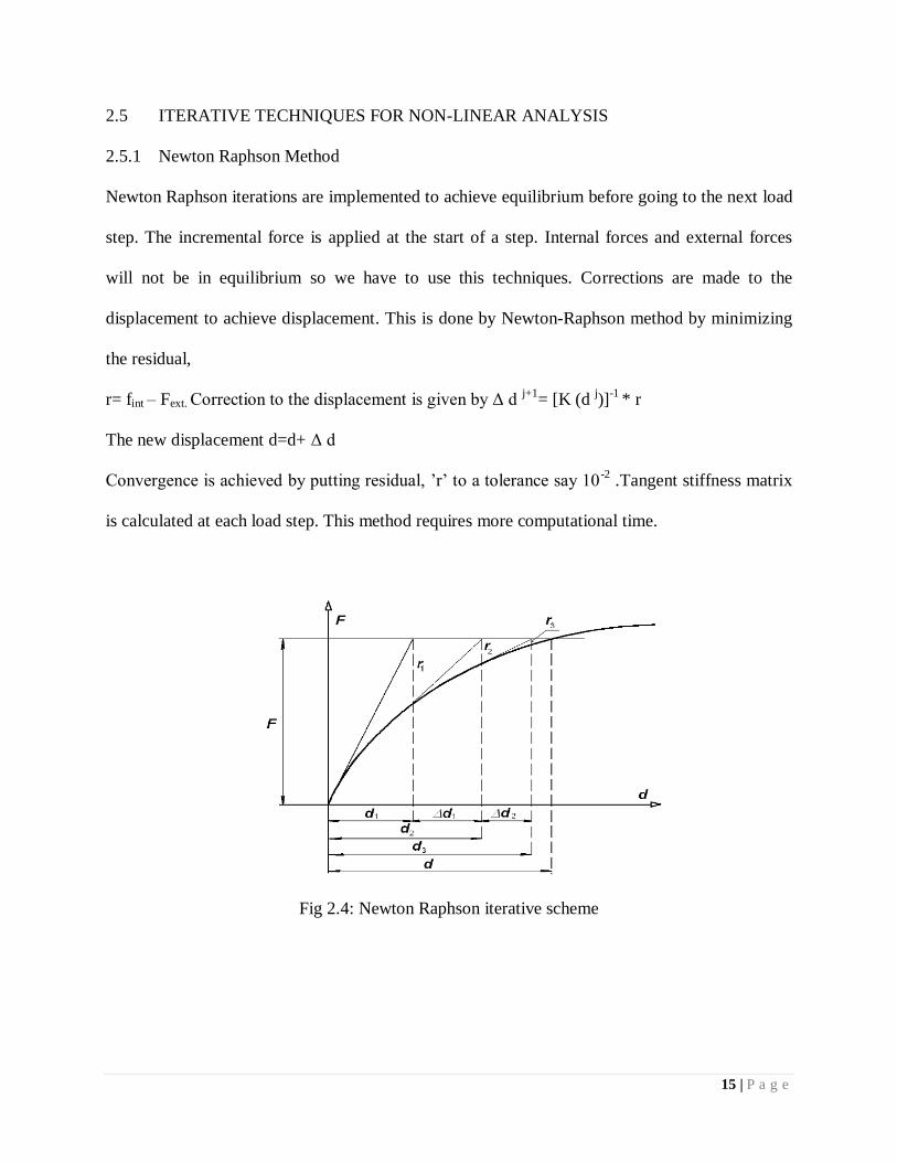
2.5.1 Newton Raphson Method

Newton Raphson iterations are implemented to achieve equilibrium before going to the next load

step. The incremental force is applied at the start of a step. Internal forces and external forces

will not be in equilibrium so we have to use this techniques. Corrections are made to the

displacement to achieve displacement. This is done by Newton-Raphson method by minimizing

the residual,

r= fint – Fext. Correction to the displacement is given by Δ d j+1

= [K (d j)]

-1 * r

The new displacement d=d+ Δ d

Convergence is achieved by putting residual, ’r’ to a tolerance say 10-2

.Tangent stiffness matrix

is calculated at each load step. This method requires more computational time.

Fig 2.4: Newton Raphson iterative scheme

16 | P a g e

2.6 CONFINEMENT MODELS FOR CONCRETE

Capacity of RC sections can be significantly increased by confining the concrete with confining

stirrups. Strength and strain capacity is increased due to the restrain of dilation of the concrete in

compression. Confining action comes into play when the concrete is in compression and core

expands against transverse reinforcement. In highly seismic region, the increase in strength and

ductility is an important aspect for the design of RC structural elements. Confinement

characteristics of concrete can be shown in stress stain curves. A review of confinement models

are given below

2.6.1 MANDER et al. (1988) MODEL

This model first investigated different cross section columns to study the impact of transverse

reinforcement. It was found that the performance over the complete stress-strain range was same

if the peak strain and stress coordinates might be found ( , ′). The Mander et al. (1988)

model is popular and in this study we account material nonlinearity from this model.

The peak stress,

(2.1)

Where ′ is unconfined compressive strength equal to 0.75 , is the confinement

effectiveness coefficient having a typical value of 0.95 for circular sections and 0.75 for

rectangular sections, = Volumetric ratio of confining steel, ℎ= Grade of confining steel,

Strain corresponding to peak stress,

(2.2)

The ultimate compressive strain,

17 | P a g e

(2.3)

Where = Steel strain at maximum tensile stress,

The stress at any strain,

(2.4)

(2.5)

Fig 2.5: Mander et al 1988 model

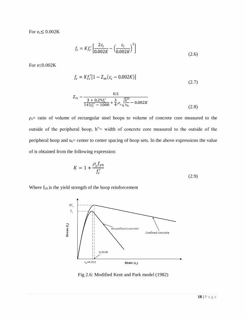
2.6.2 MODIFIED KENT AND PARK MODEL (1982)

The strength enhancement factor, K was expressed in terms of volumetric ratio of confining

reinforcement was introduced to existing Kent and park model (1971). This model of stress

strain is also taken for the study.

18 | P a g e

For ec 0.002K

(2.6)

For e≤0.002K

(2.7)

(2.8)

ρs= ratio of volume of rectangular steel hoops to volume of concrete core measured to the

outside of the peripheral hoop, h”= width of concrete core measured to the outside of the

peripheral hoop and sh= center to center spacing of hoop sets. In the above expressions the value

of is obtained from the following expression:

(2.9)

Where fyh is the yield strength of the hoop reinforcement

Fig 2.6: Modified Kent and Park model (1982)

19 | P a g e

2.6.3 IS 456 (2000) MODEL

IS 456 (2000) assumes the same ductility and strength for both confined and unconfined concrete

.The maximum value of strain considered is 0.0035.IS 456 (2000) model underestimates the

ductility and strength of the RC sections. The stress strain relationship is given by

(2.10)

(2.11)

where is the stress in concrete corresponding to the strain and ′ is the strength concrete

corresponding to the strain 0.002 ( ).

Fig 2.7: IS 456 model (2000)

20 | P a g e

2.6.4 NON LINEAR STEEL MODEL

The bilinear elastic-plastic portion followed by a strain hardening region shown in Lee and

Mosalam,(2004) calculated by

(2.12)

Where fs is the steel stress corresponding to the steel strain es,

fy is the yield stress, fu is the ultimate stress, esh is the strain at the on-set of hardening,

and esu is the ultimate strain.The fig 2.6 shows the stress strain relationship for the steel

Fig.2.8: Reinforcing steel constitutive model (Lee and Mosalam, 2004)

2.7 MONTE CARLO SIMULATION

Shinozuka et al. (1972) reported that the importance of variability of the material properties for

estimating the strength of RC structures. Monte Carlo simulation is an oldest computational

approach used in several studies of RC sections such as beams and columns.

Reliability of a RC beams were studied by Knappe et al. (1975). Strength analyses of RC beam-

column members by considering variability of material properties and dimensions were studied

21 | P a g e

by Grant et al.(1978), Mirza and MacGregor (1975), and Frangopol et al. (1975). Probabilistic

estimation of RC frames were done by Chryssanthopoulos et al. (1975), Dymiotis et al. (1975),

Ghobarah and Aly (1975), and Singhal and Kiremidjian (1996) recently proposed systematic

ways of evaluating RC framed structures by considering the uncertainty of ground motions and

the material variability. Ghobarah and Aly (1998) accounted for uncertainties in member

dimensions.

22 | P a g e

2.8 SUMMARY

This Chapter briefly describe previous studies on distributed inelasticity models, numerical

integration, solution strategies and iterative techniques for nonlinear analysis. The present study

uses various confinement models and hence a description of confinement models for the concrete

such as Mander et al. (1988) etc are also discussed in detail. Third part of the Chapter discussed

the studies employing Monte Carlo simulation. A simple and convenient model for nonlinear

analysis of RC sections is required for the probabilistic analysis in this study. The classical

displacement based - stiffness method used by Lee and Mosalam (2004) is found to be simple

and easy to implement for the present study.

23 | P a g e

3 ELEMENT FORMULATIONS

24 | P a g e

CHAPTER-3

ELEMENT FORMULATIONS

3.1 GENERAL

Present study uses the distributed inelasticity approach based on the fiber element approach for

nonlinear structural analysis. The fiber element can be used with two main formulations, namely,

displacement-based (DB) stiffness method, which is the classical finite element formulation, and

the force-based flexibility (FB) method. The DB formulation uses displacement shape functions,

while the FB formulation uses internal force shape functions. This Chapter discuss the

formulations and step wise procedure for the DB and FB method in detail.

3.2 DISPLACEMENT BASED-STIFFNESS METHOD

The displacement based-Stiffness method uses displacement interpolation function. It accounts

for axial and transverse displacements of the elements. Linear Lagrangian shape function and

cubic hermitian polynomial are the most used shape function for the beam-column elements. The

element formulation of stiffness based models are comparatively easy when compared to

flexibility based models.

The element force and deformation vectors are given by

p= [p1, p2, p3, ….p6]T (3.1)

u= [u1, u2, u3,…u6]T (3.2)

The section force and deformation vector is given by

q(x)= [ N(x), M(x)]T

(3.3)

Vs(x)= [ ε0(x), ϕ(x) ]T (3.4)

25 | P a g e

Where N is the axial force, M is the bending moment, ε0 is axial strain and ϕ is the curvature with

respect to section position ‘x’. Figure 3.2 depicts the element force and deformations

Fig 3.1: Element force and deformations

The strain increment in the ‘ith

’ fiber is given by

dεi= as(y) dVs(x) (3.5)

where as(y)= [1 –yi] and dVs(x)= [ dε0(x), dϕ(x) ]T

where yi is the distance between the coordinate reference axis and ith

fiber

Section deformation are found from strain deformation relationship that is

n+1 (3.6)

un+1 = un + ∆u is the element deformation vector at the load step n+ 1,

B(x) , G(x) ,C(x) is the strain-deformation transformation matrices

G(x)= (3.7)

The section stiffness matrix k(x) can be computed as

(3.8)

Where E(x,y) is the tangent stiffness matrix

The section resisting force can also be determined by

(3.9)

26 | P a g e

The element stiffness matrix Ke

(3.10)

The element resisting vector re

(3.11)

Where

T(x) = B(x) + G(x), Transformation matrix

N (x) is a component of r (x) representing the axial force resultant and L is the element length

For nonlinear analysis, we use ∆p = ke ∆u

3.3 FLEXIBILITY BASED-FORCE METHOD

The Flexibility based-force method uses force interpolation function. In this formulation,

element equilibrium is satisfied in strict sense. The implementation is quite challenging as

existing finite element program generally uses stiffness formulations. The element formulation of

flexibility based models are comparatively accurate when compared to flexibility based models.

b(x) is the force interpolation function used for element state determination.

Element state determination

Step 1: Compute structural displacements and update

(3.12)

p=p+Δp (3.13)

Step 2: Compute Element deformations and update

Δq=Lele × Δp (3.14)

q=q+Δq (3.15)

Lele=Transformation matrix

Step 3: Compute Element force and update

27 | P a g e

(3.16)

Q=Q+ΔQ (3.17)

Step 4: Compute section force and update

ΔDx=b(x) Q (3.18)

Dx=Dx+ΔDx (3.19)

Step 5: Compute section force and update

Δdx=f ΔD(x) r(x) (3.20)

dx=dx+Δdx (3.21)

Step 6: Compute fiber stresses and tangent modulus from constitutive stress –strain curve

Step 7: Compute new section flexibility matrix

(3.22)

Where f=[k(x)]-1

Step 8: Compute section resisting forces

(3.23)

Step 9: Compute Unbalanced force

Du=Dx-DR(x) (3.24)

Step 10: Compute residual section deformation

r(x)=f(x) Du (3.25)

Step 11: Compute Flexibility matrix

28 | P a g e

(3.26)

Where Flexibility,F=[ K]-1

Step 12: Check for convergence

Case 1: If Qi=Qj , Ki=Kj then the element converged

Case 2: If element not converged

(3.27)

and Δq=-s

Step 12: Compute structure stiffness and resisting forces

PR=LeleT Qele (3.28)

Ks= LeleT Kele Lele

T (3.29)

3.1 SUMMARY

This Chapter presents the formulation and step wise procedure for the both the DB and FB

method. This steps are implemented in the MATLAB 2012b for nonlinear analysis of RC

sections and probabilistic analysis further.

29 | P a g e

4 IMPLEMENTATION OF FIBER ELEMENT FOR

PROBABILISTIC ANALYSIS

30 | P a g e

CHAPTER-4

IMPLEMENTATION OF FIBER ELEMENT FOR PROBABILISTIC

ANALYSIS

4.1 GENERAL

First part of this Chapter presents a flow chart that explains both the stiffness based method

(DBM) and flexibility based methods (FBM) using fiber formulation for nonlinear analysis.

Examples of a RC column section involving material nonlinearity is considered and analyses are

conducted. Second part of this Chapter illustrate the results of these analyses and its comparison

with exact results. Constitutive stress strain relations for concrete and steel reinforcement are

incorporated in fiber formulation to obtain the nonlinear responses. Probabilistic analysis

incorporating uncertainties in the material and geometric parameters properties of RC section, is

carried out in the last part of this chapter.

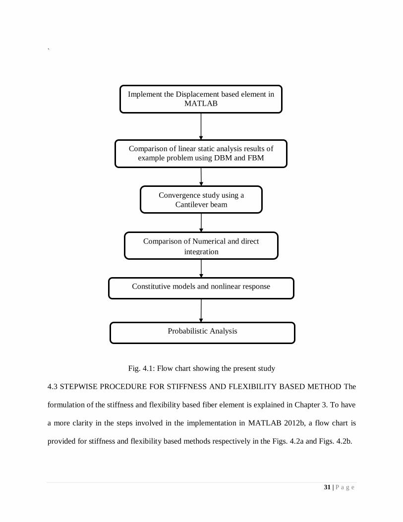
4.2 METHODOLOGY

The flow chart of the different phases of the presented such as, comparison of DBM and FBM

using linear static analysis, convergence study, discussion of numerical and direct integration

method, nonlinear analysis using different confinement models, and a probabilistic analysis

using the implemented model in MATLAB 2012b is displayed in Fig.4.1.

31 | P a g e

`

Fig. 4.1: Flow chart showing the present study

4.3 STEPWISE PROCEDURE FOR STIFFNESS AND FLEXIBILITY BASED METHOD The

formulation of the stiffness and flexibility based fiber element is explained in Chapter 3. To have

a more clarity in the steps involved in the implementation in MATLAB 2012b, a flow chart is

provided for stiffness and flexibility based methods respectively in the Figs. 4.2a and Figs. 4.2b.

Comparison of linear static analysis results of

example problem using DBM and FBM

Implement the Displacement based element in

MATLAB

Convergence study using a

Cantilever beam

Comparison of Numerical and direct

integration

Constitutive models and nonlinear response

Probabilistic Analysis

32 | P a g e

Fig 4.2a: Flow chart of state determination of Stiffness based method

33 | P a g e

Fig 4.2b: Flow chart of state determination of Flexibility based method

4.4 COMPARISON OF LINEAR ANALYSIS USING DB AND FB FORMULATION

4.4.1 Elastic Column with Axial Force

An elastic column having 2m length and a cross section of 100mm x 300mm is chosen. Axial

compressive load is considered at the free end. The details of the column, cross section and the

34 | P a g e

constitutive linear relationship of the fiber element is provided in the Fig.4.3. The cross section is

discretized as fiber element. The details of fiber discretization followed for both DBM and FBM

are presented in the Table 4.1. Stiffness matrices at the section level and global level are

computed as per both the DBM and FBM. The displacement is incrementally applied till a target

displacement and the force and the displacement at the free end is monitored in each step for

both the type of formulations. A comparison is done for both displacement based method and

flexibility based method by using fiber element method. The force versus displacement responses

from both DBM and FBM are illustrated in the Fig. 4.4. It can be seen the linear responses from

both the approaches are matching. Hence this implemented model can be used for further

parametric studies.

Fig 4.3: Homogenous column subjected to axial compression

Table 4.1: Parameters for number of fiber elements

No. of fiber in y direction 20

No. of fiber in z direction 20

35 | P a g e

Fig 4.4: Force Displacement response for Elastic Column using DBM and FBM

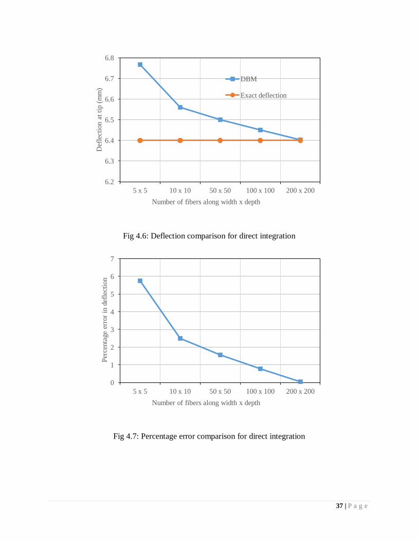
4.5 CONVERGENCE STUDY - DIRECT INTERATION

The number of fiber elements in a section may influence the responses. In order to estimate the

optimum number of fiber elements for reasonably accurate results, a convergence study is

required to be conducted. A cantilever beam with 400 mm length with a cross section of 20mm x

20mm is chosen a load of 100N is applied at the free end. The linear constitutive relationship is

considered for all the fiber elements as shown in the Fig. 4.4. The number of fibers (in both

width and depth directions) and number of integration sections are treated as variables. The

linear static analysis is conducted to find the displacement at free end for different number of

fibers. The displacement at free end obtained for each case is tabulated in the Table 4.2. The

deflection at free versus number of fibers is plotted in the Fig. 4.6. The percentage error versus

number of fibers is expressed graphically in Fig. 4.7. It can be seen that the number of fibers in

the cross section increases to 200 x 200 and the number of integration section sections to 400,

and the deflection tends to converge to 6.40 mm. About 400 number of sections is required to

have convergence in the case of direct integration method.

36 | P a g e

Fig 4.5: Cantilever beam with point load at the end

Table 4.2: Convergence study - Direct integration

Fibers

Number of

Integration

Section

(Nos.)

Deflection

using DBM

(mm)

Exact

deflection

(mm)

Error

(%)

Execution

time (s)

5 x 5 25 6.77 6.40 5.75 16

10 x 10 50 6.56 6.40 2.50 16

50 x 50 100 6.50 6.40 1.56 16

100 x 100 200 6.45 6.40 0.78 17

200 x 200 400 6.40 6.40 0.05 28

37 | P a g e

Fig 4.6: Deflection comparison for direct integration

Fig 4.7: Percentage error comparison for direct integration

6.2

6.3

6.4

6.5

6.6

6.7

6.8

5 x 5 10 x 10 50 x 50 100 x 100 200 x 200

Def

lect

ion a

t ti

p (

mm

)

Number of fibers along width x depth

DBM

Exact deflection

0

1

2

3

4

5

6

7

5 x 5 10 x 10 50 x 50 100 x 100 200 x 200

Per

centa

ge

erro

r in

def

lect

ion

Number of fibers along width x depth

38 | P a g e

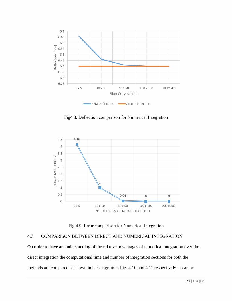
4.6 CONVERGENCE STUDY - NUMERICAL INTEGRATION

In order to estimate the optimum number of fiber elements for the numerical integration using

Gauss Lobatto, the same cantilever beam problem as that of the previous convergence study is

considered. The linear constitutive relationship considered is the same as shown in the Fig. 4.5.

The number of fibers (in both width and depth directions) and number of integration points are

treated as variables. The linear static analysis is conducted to find the displacement at free end

for different number of fibers. The displacement at free end obtained for each case is tabulated in

the Table 4.3. The deflection at free end versus number of fibers is plotted in the Fig. 4.8. The

percentage error versus number of fibers is expressed graphically in Fig. 4.9. It can be seen that

the number of fibers in the cross section increases to 50 x 50 and the number of integration

section sections to 3, and the deflection tends to converge to 6.40 mm. It can be seen that only

about 5 number of sections (instead of 400 in the case of direct integration) is required to have

convergence in the case of direct integration method.

Table 4.3: Numerical integration: Fiber cross sections-Deflections and errors

Fibers

Number of

Integration

Section

(Nos.)

Deflection

using DBM

(mm)

Exact

deflection

(mm)

Error

(%)

Execution

time (s)

5 x 5 3 6.66 6.40 4.16 2

10 x 10 3 6.46 6.40 1.00 2

50 x 50 3 6.41 6.40 0.04 2

100 x 100 5 6.40 6.40 0 2

200 x 200 5 6.40 6.40 0 2

39 | P a g e

Fig4.8: Deflection comparison for Numerical Integration

Fig 4.9: Error comparison for Numerical Integration

4.7 COMPARISON BETWEEN DIRECT AND NUMERICAL INTEGRATION

On order to have an understanding of the relative advantages of numerical integration over the

direct integration the computational time and number of integration sections for both the

methods are compared as shown in bar diagram in Fig. 4.10 and 4.11 respectively. It can be

6.25

6.3

6.35

6.4

6.45

6.5

6.55

6.6

6.65

6.7

5 x 5 10 x 10 50 x 50 100 x 100 200 x 200

Def

lect

ion

(mm

)

Fiber Cross section

FEM Deflection Actual deflection

4.16

1

0.04 0 0

0

0.5

1

1.5

2

2.5

3

3.5

4

4.5

5 x 5 10 x 10 50 x 50 100 x 100 200 x 200

PER

CEN

TAG

E ER

RO

R %

NO. OF FIBERS ALONG WIDTH X DEPTH

40 | P a g e

observed that the numerical integration is found to be more efficient due to computational

efficiency.

Fig 4.10: Number of fiber comparison for both integrations

Fig 4.11: Execution time comparison for both integrations

4.8 CONFINEMENT MODELS IN NON-LINEAR RESPONSE

The effect of confinement in the concrete play a major role in the nonlinear response of frames.

To study the effect of confinement models in the response, the fiber elements are considered to

have constitutive relationship of confinement concrete in the core region (region over which the

25

50

100

200

400

3

3

3

5

5

0 100 200 300 400 500

5 x 5

10 x 10

50 x 50

100 x 100

200 x 200

No. of integration section

Fib

er C

ross

-sec

tion

Number of integration Section :Numerical Integration

16

16

16

17

28

2

2

2

2

2

0 5 10 15 20 25 30

5 x 5

10 x 10

50 x 50

100 x 100

200 x 200

Time (s)

Nu

mb

er o

f fi

bers

Execution time (s):Numerical Integration Execution time (s):Direct Integration

41 | P a g e

concrete is confined due to the transverse reinforcements) and unconfined region (region over

which there is no confinement for the concrete) in the cover concrete.

4.9 RC COLUMN WITH AXIAL COMPRESSION

An RC column having dimensions 350 mm x 350mm with reinforcement detailing as shown in

Fig. 4.15 is considered. To have the prominent effect of confinement, the transverse

reinforcement in the column is assumed as high as 16mm dia @ 85 mm c/c. The confined and

unconfined stress strain curves obtained for the above transverse reinforcement is calculated as

per the expressions for various confinement models namely Mander et al. (1988), Modified Kent

and Park model (1982), IS 456(2000) as given in the Chapter 2.

Nonlinear model of the cross section is developed using the implemented displacement based

fiber element method. The RC column cross section is discretized to number of fibers, and for

each fiber, depending on its location whether in core region or cover region, the corresponding

confined and unconfined constitutive relations are used. The fibers at the locations of main

reinforcement is modelled using the constitutive relation for the steel. Nonlinear analysis is

conducted using displacement control method to obtain the force and displacement responses at

the free end. The force –displacement curves obtained using Mander et al. (1988) is shown in

Fig. 4.13(a). Fig. 4.16(b) and (c) shows the uniaxial constitute relations used for fibers at

confined and unconfined regions respectively. The maximum axial force for this model is

obtained as about 5000kN.

To study the effect of not considering confinement in core region, the above RC section is

remodelled by assuming the unconfined stress strain curve for the core region. The

corresponding axial force versus displacement is shown in the Fig. 4.14a. The stress strain

relationship used for the concrete and steel is also shown in Fig. 4.14b and 4.14c.

42 | P a g e

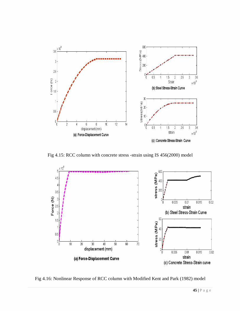
IS 456 (2000) recommend stress strain curve of concrete to be considered for the limit state

design of RC sections. Axial force versus displacement relationship is obtained as shown in the

Fig. 4.15a. The stress strain relations for the steel and concrete are shown in Figs. 4.15b and

4.15c.

Force displacement relationship for the same RC cross section is obtained using the confinement

model as per Kent and Park (1982). The force versus displacement responses and the

corresponding stress strain curves used as shown in Fig. 4.16a, 4.16b and 4.16c respectively.

A comparison of axial force versus displacement curves for all the four case discussed in this

section is shown in Fig. 4.17. It can be seen the Mander et al. (1988) predicts higher values for

strength compared to other models. This is due to high value of confinement factor values. The

maximum compressive strain by IS 456 (2000) is 0.0035. It can be seen that IS 456(2000) model

has less ductility when compared to other models due the relative low value of maximum strain.

43 | P a g e

Fig 4.12: RC Column subjected to different stress strain models

width 350 mm

depth 350 mm

clear cover 40 mm

Main steel dia 25 mm

Stirrup dia 16 mm

Area of stirrups along X 402 mm2

core width 270 mm

Area of stirrups along Y 402 mm2

spacing 85 mm

Reinforcement ratio, 0.02 mm2

X direction, ρsx

Reinforcement ratio, 0.02 mm2

Y direction, ρsy

Reinforcement ratio ρs 0.04 mm2

Characteristic_compressive

strength,fck 25 MPa

f΄co 18.8 MPa

Yield Strength, fy 415 MPa

Cross section details of Column

44 | P a g e

Fig 4.13: RCC column modelled with confined and unconfined sections using Mander et. al,

(1988)

Fig 4.14: RCC column, entire section modelled as unconfined concrete as per Mander et al.

(1988)

45 | P a g e

Fig 4.15: RCC column with concrete stress -strain using IS 456(2000) model

Fig 4.16: Nonlinear Response of RCC column with Modified Kent and Park (1982) model

46 | P a g e

Fig.4.17: Comparison of force versus deformation of RC column with axial loading using

different confinement models for concrete

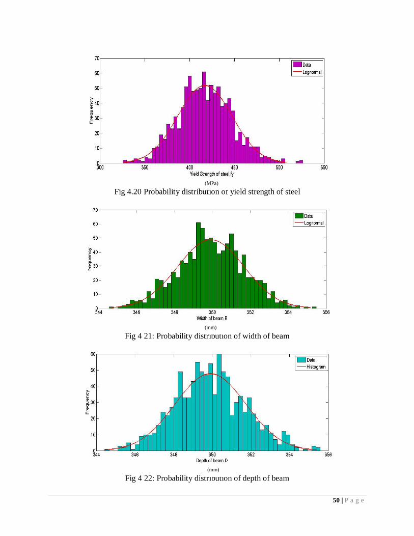
4.10 PROBABILISTIC STUDY OF NONLINEAR RESPONSE

The methodology followed for the probabilistic analysis of RC sections is shown below. The

present study consider the variables, compressive strength of concrete, yield strength of steel,

initial tangent modulus of steel and concrete and dimensions of the member as random variables.

The cross section and member shown in Fig.4.12 is considered for the probability analysis. Each

random variable is treated as uncorrelated and 1000 samples have taken for the monte carlo

simulation. The probability distributions of each variable considered are lognormal and the

statistical details of the variables are given in the Table 4.5. The probability distributions of each

random input variables that define the computational models is presented in the Figs. 4.20 to

4.26.

0

1000

2000

3000

4000

5000

6000

1 2 3 4 5 6 7 8 9 1 0 1 1 1 2 1 3 1 4 1 5 1 6 1 7 1 8 1 9 2 0 2 1

FOR

CE

(KN

)

DISPLACEMENT (MM)

Mander et al. - full section unconfined Mander et al. Kent and Park (1982) IS456 (2000)

47 | P a g e

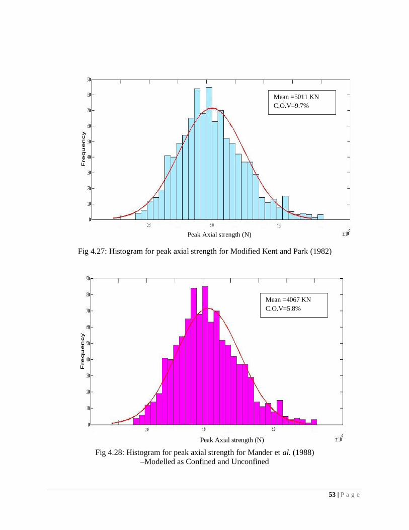
For each of the random samples of the above variables, displacement based finite element

models are developed to conduct nonlinear analysis. The nonlinear response curves from

probabilitistic analysis, histograms for peak axial strength and its probability distributions are

found out. The Figs. 4.27, 4.28, 4.29 and 4.30 shows the probability distributions for peak axial

strength for all the confinement conditions, namely, namely Mander et al. (1988), Modified Kent

and Park model (1982), IS 456(2000). The mean and C.O.V. for the peak strength for each case

is shown in the respective Figs. The coefficient of variations of all the input random variables

and the peak axial strength response is summarized in a graphical form in Fig. 4.32. It can be

seen that the C.O.V of the peak strength varies between 5.8 to 9.3%, when the C.O.V of input

random variables is about 0.5 to 15%.

48 | P a g e

Fig 4.18: Flow chart of the probabilistic fiber element approach

Run non-linear Analysis

Steel Young’s Modulus

Steel Yield Strength

Young’s Modulus of

Concrete

Compressive strength of

concrete

Yield strength of confinement

bars (DBM) Fiber element

Model description

Obtain structural response in

terms of Force Displacement plot

displacemen

Geometric Properties of beam

and column

Sampling variables

Determination of Maximum force in the

structure

Histogram and Probabilistic distribution and

response parameters

49 | P a g e

Table 4.4: Parameters and distributions used for generation of random variables

Random

variable Parameters

Probability

distribution

function

Mean C.O.V

(%) Reference

Characteristic

compressive

strength

fck Lognormal 25MPa 15 Devandiran

et.al.(2013)

Yield Strength

of steel fy Lognormal 415MPa 7.6

Devandiran

et.al.(2013)

Column

Width

Lognormal

350mm 0.5

Assumed Depth 350mm 0.5

Length 4000mm 0.5

Initial Tangent

Modulus of

Concrete

Ec

Lognormal

25000MPa 12

Lee and

Mosalam

(2004)

Initial Tangent

Modulus of

Steel

Es 200000MPa 7.6 Devandiran

et.al.(2013)

Fig 4.19: Probability distribution of Compressive strength of concrete.

(MPa)

50 | P a g e

Fig 4.20 Probability distribution of yield strength of steel

Fig 4 21: Probability distribution of width of beam

Fig 4 22: Probability distribution of depth of beam

(MPa)

(mm)

(mm)

51 | P a g e

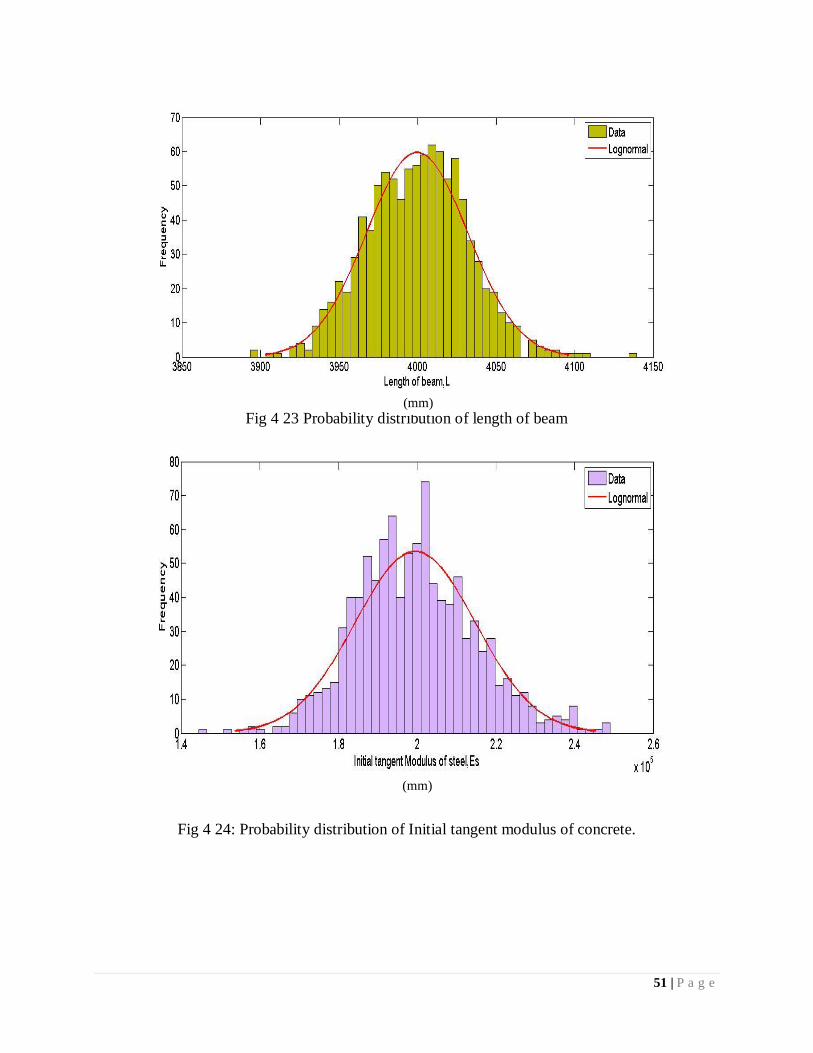
Fig 4 23 Probability distribution of length of beam

Fig 4 24: Probability distribution of Initial tangent modulus of concrete.

(mm)

(mm)

52 | P a g e

Fig 4 25: Probability distribution of initial tangent modulus of concrete.

Fig 4.26: Histogram for peak axial strength using IS 456 (2000) model

Mean =3051 KN

C.O.V=9.3%

(MPa)

Peak Axial strength (N)

53 | P a g e

Fig 4.27: Histogram for peak axial strength for Modified Kent and Park (1982)

Fig 4.28: Histogram for peak axial strength for Mander et al. (1988)

–Modelled as Confined and Unconfined

Mean =5011 KN

C.O.V=9.7%

Peak Axial strength (N)

Peak Axial strength (N)

Mean =4067 KN

C.O.V=5.8%

54 | P a g e

Fig 4.29: Coefficient of Variation (C.O.V) for all random input and response parameters using

different confinement models

4.11 SUMMARY

This Chapter discuss about the comparison of responses of a column under axial force

implemented using DBM and FBM method. The comparison for the selected problem is fairly

matching. A convergence study for two integration types namely, direct and numerical, is

conducted and discussed the advantages of numerical method. The confinement effects in RC

sections can be modelled conveniently using fiber based element. The axial force responses of

RC column is studied using various confinement models. A probabilistic analysis to

incorporating nonlinearity is also carried out to study the uncertainty in the peak axial strength

response considering the uncertainties in the sensitive input parameters.

15

7.6

12

7.6

0.5

0.5

0.5

9.3

9.7

5.8

0 2 4 6 8 10 12 14 16

Characteristic compressive strength, fck

Yield Strength, fy

Initial Tangent Modulus of Concrete,Ec

Initial Tangent Modulus of Steel,Es

Width

Depth

Length

Peak strength,IS 456

Peak strength,Modified Kent and Park (1982)

Peak strength,Mander et al(1988)

C.O.V

VA

RIA

BLE

S

55 | P a g e

5 SUMMARY AND CONCLUSION

56 | P a g e

CHAPTER 5

SUMMARY AND CONCLUSION

5.1 SUMMARY

The main objective of the present study was to implement the displacement based (stiffness)

fiber element for nonlinear analysis of RC Sections. Element formulation of both stiffness and

flexibility based fiber models were discussed. Global stiffness computation using both direct

integration and numerical integration is discussed. Popular confinement models for stress-strain

relationship for concrete were discussed and used as the constitutive relationship for fiber

element to study the nonlinear response. The uncertainty exist in the constituent material

properties of concrete needs a probabilistic analysis for realistic estimation of nonlinear

responses. A probabilistic analysis is carried out further in the implemented model using a

Monte-Carlo simulation. Major conclusions from the present study is presented in the following

section.

5.2 CONCLUSIONS

1. The force displacement responses obtained from both the DBM and FBM are found to be

same.

2. Direct integration method used for DBM required about number of sections as high as

400 compared to that of five in the case of numerical integration.

57 | P a g e

3. Confinement model as per Kent and Park et al. (1988) predicts higher values for strength

compared to other models. This is due to high value of confinement factor values.

4. As the maximum compressive strain by recommended by IS 456 (2000) is as low as

0.0035, the displacement is reduced by 61.5% when compared to other confined models

(Mander et al.(1988), Modified Kent and Park(1982) )

5. Probabilistic analysis of the RC column under axial load shows that the C.O.V of the

peak strength can vary between 5.8 to 9.7%, when the C.O.V of input random variables,

fck, fy, breadth, width, length, Ec, Es are 15%,7.6%,0.5% , 0.5% , 0.5% ,12%,7.6%

respectively..

5.3 LIMITATIONS AND FUTURE SCOPE OF WORK

The RC columns in bending is not considered in the present study. It can be extended to

RC frame sections in bending.

Geometric nonlinearity can be incorporated with material nonlinearity for RC sections.

It is learned that FBM is suitable for nonlinear problems of RC sections. The study can be

extended further to implement this.

58 | P a g e

REFERENCES

59 | P a g e

1. Chryssanthopoulos MK., Dymiotis C., Kappos AJ. Probabilistic evaluation of behaviour

factors in EC8-designed R/C frames. Eng Struct 2000;22:1028–41.

2. Dymiotis C., Kappos AJ, Chryssanthopoulos MK .Seismic reliability of RC frames with

uncertain drift and member capacity. J Struct Eng, ASCE 1999; 125(9):1038–47.

3. Filippou, F C., D’Ambrisi., A and Issa., A .Nonlinear Static and Dynamic Analysis of

Reinforced Concrete Subassemblages, Report No. UCB/EERC–92/08, Earthquake

Engineering Research Center, College of Engineering, University of California,

Berkeley, 1992.

4. Filippou F., and Issa, A.. 1988. Nonlinear analysis of reinforced concrete frames under

cyclic load reversals. Rep. No. UCB/EERC-88/12, Earthquake Engineering Research

Center, Univ. of California, Berkeley,Calif.

5. Frangopol DM., Spacone E., Iwaki I. A new look at reliability of reinforced concrete

columns. Struct Safety 1996;18(2):123–50

6. Ghobarah A, Aly NM. Seismic reliability assessment of existing reinforced concrete

buildings. J Earthquake Eng 1998;2(4):569–92

7. Grant LH, Mirza SA, MacGregor JG Monte Carlo study of strength of concrete columns.

ACI J 1978;75(8):348–58.

8. Hellesland, J and Scordelis, A [1981] Analysis of RC bridge columns under imposed

deformations, in IABSE Colloquium (Delft, Netherlands), pp. 545–559.

9. Indian Standard Plain and Reinforced Concrete – Code of Practice (4th Revision), IS 456:

2000, BIS, New Delhi.

10. Kaba, S and Mahin, S A [1984] Refined modeling of reinforced concrete columns for

seismic analysis, in Refined Modeling of Reinforced Concrete Columns for Seismic

Analysis

11. Kent D C, Park R 1971 Flexural members with confined concrete. J. Struct. Div. ST7, 97:

1969–1990

60 | P a g e

12. Knappe OW, Schue¨ller GI, Wittmann FH On the probability of failure of a reinforced

concrete beam. In: Proceedings of the Second International Conference on Application

Statistic Probabilistic in Soil Structure Engineering, ICASP, Aachen, Germany,

September, 1975, p. 153–70.

13. Lee, TH and Mosalam,KM "Probabilistic Fiber Element Modeling of Reinforced

Concrete Structures," Computers and Structures, 2004, Vol. 82, No. 27, pp. 2285-2299.

14. MATLAB Version 8.0. Natick, Massachusetts: The MathWorks Inc., 2012bb.

15. Mahasuverachai, M and Powell, G. H. [1982] Inelastic analysis of piping and tubular

structures, in Inelastic Analysis of Piping and Tubular Structures.

16. Mander JB, Priestley MJN, Park R. Theoretical stress– strain model for confined

concrete. J Struct Eng, ASCE 1988;114(8):1804–26.

17. Mari, A and Scordelis, A [1984] Nonlinear geometric material and time-dependent

analysis of three-dimensional reinforced and prestressed concrete frames. Research

report: SESM Report 82/12.

18. Mirza SA, MacGregor JG Variations in dimensions of reinforced concrete members. J

Struct Div, ASCE 1979; 105(ST4):751–66.

19. Otani, S Inelastic Analysis of RC Frame Structures, Journal of the Structural Division,

ASCE, 100 (ST7), 1433-1449,1974.

20. Park R, Priestley M J N, Gill W D 1982 Ductility of square-confined concrete columns. J.

Struct. Div. ST4, 108: 929–950

21. Spacone E, Ciampi V, Filippou F C A beam element for seismic damage analysis.

UCB/EERC-92/07. Earthquake Engineering Research Center. University of California,

Berkeley. CA, 1992

22. Spacone, E, Ciampi, V, and Filippou, F C (1996a). Mixed formulation of nonlinear beam

finite element. Comput. Struct., 58, 71-83. Spacone, E., Filippou, F. C., and Taucer, F. F.

(1996b). Fibre beam-column model for non-linear analysis of R/C frames: Part I.

Formulation. Earthquake Eng. Struct. Dyn., 25(711-725).

61 | P a g e

23. Shinozuka M Probabilistic modeling of concrete structures. J Eng Mech Div, ASCE

1972;98(6):1433–51.

24. Singhal A, Kiremidjian A Method for probabilistic evaluation of seismic structural

damage. J Struct Eng, ASCE 1996;122(12):1459–67.

25. Soleimani, D, Popov, E.P and Bertero, VV Nonlinear Beam Model for R/C Frame

Analysis, 7th ASCE Conference on Electronic Computation, St. Louis, 1979

26. Takayanagi, T and Schnobrich, WC (1979). Non-Linear Analysis of Coupled Wall

Systems, Earthquake Engineering and Structural Dynamics, Vol. 7, pp. 1-22.

27. Taucer, F, Spacone, E, & Filippou, F (1991). A fiber beam-column element for seismic

response analysis of reinforce concrete structures: University of California, Berkeley.

28. ’www.theconcreteportal.com

29. Zeris, CA and Mahin, SA (1988). Analysis of Reinforced Concrete Beam-Columns under

Uniaxial Excitations, Journal of Structural Engineering, ASCE, Vol. 114, No. 4.

30. Zienkiewicz, O C and Taylor, R L, The Finite Element Method, Volume 1, Basic

Formulation and Linear Problems, 4th Edition, McGraw-Hill, London, 1989, pp 72-80,

128-130.