Embed Size (px)
Citation preview

Implementation of Integral based Digital CurvatureEstimators in DGtal∗
David Coeurjolly1, Jacques-Olivier Lachaud2, Jeremy Levallois1,2
1 Universite de Lyon, CNRSINSA-Lyon, LIRIS, UMR5205, F-69621, France.
2 Universite de Savoie, CNRSLAMA, UMR5127, F-73776, France.
[email protected], [email protected], [email protected]
Abstract In many geometry processing applications, differential geometric quantities esti-mation such as curvature or normal vector field is an essential step. In [1], we have definedcurvature estimators on digital shape boundaries based on Integral Invariants. In this paper,we focus on implementation details of these estimators.
Keywords: Digital geometry, curvature estimation, integral invariants
1 Introduction
In many shape processing applications, the estimation of differential quantities on the shape bound-ary such as normal vectors, curvatures or principal directions are crucial. When evaluating adifferential estimator on discrete or digital data, because of digitization approximation, we needa way to mathematically link the estimated quantity to the expect Euclidean one. In DigitalGeometry, we usually consider multigrid convergence principles: when the shape is digitized on agrid with resolution tending to zero, the estimated quantity should converge to the expected one[2].
In [1], we have proposed digital versions of integral invariant estimators for which convergenceresults can be obtained when the kernel size tends to zero. In this paper, we first remind thegeneral principle of [1]. Then we focus on implementation details of these estimators in DGtallibrary, and finally we show some results.
1.1 Principle
In geometry processing, interesting mathematical tools have been developed to design differentialestimators on smooth surfaces based on integral invariants. The principle is simple: we move aconvolution kernel along the shape surface and we compute integrals on the intersection betweenthe shape and the convolution kernel, as follow in dimension 3:
Vr(x)def=
�
Br(x)χ(p)dp (1)
where Br(x) is the Euclidean ball of radius r, centered at x and χ(p) the characteristic functionof X . In dimension 2, we simply denote Ar(x) such quantity (represented in orange color on Fig.1).
∗This work has been mainly funded by DigitalSnow ANR-11-BS02-009 research grants
27

x
Br(x)
X
x xx
∂X Br(x)
∂X
x
∂hX
x
πXh (x)
h
Figure 1: Integral invariant computation in dimension 2 (left) and 3 (middle), and notations indimension 2 (right)
Authors of [4][5] have demonstrated that some integral quantities provide interesting curvatureinformation when the kernel size tends to zero. Indeed, thanks to Taylor expansion at x of thesurface ∂X approximated by a parametric function y = f(x) in 2d and z = f(x, y) in 3d andwith a fixed radius r, we obtain convergent local curvature estimators κr(X,x) and Hr(X,x) ofquantities κ(X,x) and H(X,x) respectively:
κr(X,x)def=
3π
2r− 3Ar(x)
r3, Hr(X,x)
def=
8
3r− 4Vr(x)
πr4(2)
κr(X,x) = κ(X,x) +O(r), Hr(X,x) = H(X,x) +O(r) (3)
where κr(X,x) is the 2d curvature of ∂X at x and Hr(X,x) is the 3d mean curvature of ∂X at x.In [1], we were interested in studying the behavior of integral invariants in digital geometry
using a multigrid framework with digitization on grids with grid step h tending to zero. We definea digital version of Eq. (2) and (3) estimators.
∀0 < h < r, κr(Z, x, h)def=
3π
2r−
3�Area(Br/h(1h · x) ∩ Z, h)
r3. (4)
where κr is an integral digital curvature estimator of a digital shape Z ⊂ Z2 at point x ∈ R2 andstep h. Br/h(
1h · x)∩Z, h) means the intersection between Z and a Ball B of radius r digitized by
h centered in x.In the same way, we have in 3d:
∀0 < h < r, Hr(Z�, x, h)
def=
8
3r−
4�Vol(Br/h(1h · x) ∩ Z �, h)
πr4. (5)
where Hr is an integral digital mean curvature estimator of a digital shape Z � ⊂ Z3 at pointx ∈ R3 and step h.
We have demonstrated that Eq. (4) and (5) are multigrid convergent. With hypothesis aboutthe shape geometry and the radius of the convolution kernel, we guarantee a theoretical conver-gence speed in O(h
13 ), confirmed with experimental results. We have also discussed about an
integral digital Gaussian curvature and principal curvature directions estimators obtained by dig-ital approximation of the covariance matrices on Eq. (1) integral. Convergence results rely onthe fact that digital moments converge in the same manner as volumes [3]. Note that as otherconvolution estimators, results of our algorithm depend on the size of the convolution kernel.
2 Implementation in DGtal
We have implemented integral invariant curvature estimators in DGtal library. DGtal is an open-source C++ library that provides geometry structures, algorithms and tools for digital data(http://libdgtal.org). Project DGtal gathers in a unified setting many data structures andalgorithms of digital geometry and related fields (digital topology, image processing, discrete ge-ometry, arithmetic). For example, DGtal provides us parametric or implicit multigrid shape con-struction in dimension 2 and 3, as well as object loaders. Furthermore, we benefit from availableimplementations of existing 2d curvature estimators. It allows us to make comparisons easy.
28

In our framework, objects are embedded into a Khalimsky space topological model. Thistopological structure gives us cells from 0 to n dimension (in 3d, cells are called pointels, linels,pixels and voxels for respectively cells of dimension 0, 1, 2 and 3). We call surfels cells of n − 1dimension and spel cells of n dimension. Khalimsky cells are defined into a Khalimsky Domain(cubical grid). For more information about the topology in DGtal, please refer to documentation(http://libdgtal.org/doc/stable/packageTopology.html)
2.1 User interface
The user part is rather simple by using only IntegralInvariantMeanCurvatureEstimator orIntegralInvariantGaussianCurvatureEstimator. These classes are parametrized by a Khal-imsky space of a digital shape and a functor who return a value for a given Khalimsky cell. Indeed,the χ(p) characteristic function is defined as a functor (here with values in {0, 1} for each spel ofthe Khalimsky space).
At initialization (init()), we specify the current grid step h, and an Euclidean radius re inorder to construct the convolution kernel. As described in Sect. 3, this parameter re determinesthe level of feature detected by the estimator.
For the evaluation (eval()), the user has two possibilities: evaluate the curvature at a specificsurfel of the digitized shape surface, or at a range of surfels. This choice can be importantbecause optimizations are available with the second option (see in Sect. 2.2). For the first one,the estimator return a curvature value at the given surfel. If you choose the second possibility,the estimator will try to optimize computations by using previous results thanks to displacementkernel masks. But it requires to set a range of 0-adjacent surfels. If the range of surfels does notfollow that rule, no optimization is performed.
2.2 Implementation details
The following paragraph gives details on IntegralInvariantMeanCurvatureEstimator andIntegralInvariantGaussianCurvatureEstimator classes.
To sum up, we need a convolution kernel which will be integrated along a digitized shapeboundary. At initialization, we first create a convolution kernel (Ball2D in 2d, Ball3D in 3d) ofEuclidean radius re and digitized at the grid step h. DigitalSurfaceConvolver is in charge ofcentering the convolution kernel on the surfel on the digitized shape border. Its objective is tocompute Br/h(
1h · x) ∩ Z and Br/h(
1h · x) ∩ Z � from Eq. (4) and (5).
At evaluation, it will place the convolution kernel in order to lie his center with the cell toestimate. After, it will iterate on all spels of the kernel, and compute the integral:
V (x) =�
spel∈Br/h(1h ·x)∩Z
f(x)g(s− x) (6)
where x is the current spel, f is the shape functor (set by user), g is the kernel functor (return1 on all spels from the kernel). IntegralInvariantMeanCurvatureEstimator uses this result to
get �Area(Br/h(1h ·x)∩Z, h) in 2d and �Vol(Br/h(
1h ·x)∩Z �, h) in 3d. With Eq. (4) and (5), it finally
returns curvature quantities. Using this approach, we obtain a computation cost in O((r/h)d) persurface element.
For IntegralInvariantGaussianCurvatureEstimator, the initialization is the same but atevaluation DigitalSurfaceConvolver computes a covariance matrix of Br/h(
1h · x) ∩ Z �. Eigen-
vectors and eigenvalues analysis of this covariance matrix helps us to extract principal curvaturesinformation. We can easily obtain mean or Gaussian curvature from them.
When we move the convolution kernel to 0-adjacent cells, we see that only few cells need tobe updated from the previous convolution. As seen in the top left illustration of Fig. 2, only thegreen and the red part are interesting, the grey part is the same from the previous result. Thiseffect can produce a lot of computations, so we only need to remove the green part, and add thered one (by additivity of the convolution).
29

�Area(Br/h(1
h· x+ �δ) ∩ Z, h) = �Area(Br/h(
1
h· x) ∩ Z, h)
− �Area(B1r/h(1
h· x) ∩ Z, h)
+ �Area(B2r/h(1
h· x+ �δ) ∩ Z, h).
where �δ is a translation vector in 0-adjacency, B1r/h is the mask to remove, and B2r/h the mask
to add (both depending to �δ).We pre-compute at initialization of estimators a set a displacement masks from the full convo-
lution kernel (see Fig. 2 at right for an example in 2d). At evaluation, we use the full kernel forthe first computation. If the next surfel is adjacent to the previous one, we use a pair of masks(depending to the shift) to remove/add interested quantities to the last. In the worst case, allsurfels set by user to the estimator are not adjacent and it will compute the curvature alwayswith the full convolution kernel, which means no optimizations. The computation cost per surfaceelement can be reduced from O((r/h)d) (size of the complete kernel) to O((r/h)d−1), and theextra-cost of pre-computing displacement masks is meaningless: for example, with a full 2d kernelsupport size of 91893, the optimization built 8 supplementary masks of size ≈ 450.
Figure 2: Illustration of the optimization with partial masks of a 2d ball for a given h. On the
top left: Illustration of a displacement of a full kernel from x to x+ �δ, on the bottom left: full 2d
kernel support, on the right: 0-adjacent 2d partial displacement masks of full kernel support.
3 Results
For all results presented in this section, yellow color is the highest curvature value, blue is thelowest curvature value, and red means in-between max and min values. In Fig. 3, we can seein order mean and Gaussian curvature mapped in a blobby cube1. We can also extract principalcurvature information. As mentioned before, the user needs to choose a convolution kernel sizere, which will influence the level of details captured (see Fig. 3) and computation time.
Euclidean radius re of a convolution kernel determines the level of details of estimated curva-ture. It is an intuitive behavior, because a smaller convolution kernel will be more influenced bysmall features, but will ignore large features and dependent to the noise level. A larger convolutionkernel will result the opposite effect.
1Implicit surface is 81x4 + 81y4 + 81z4 − 45x2 − 45y2 − 45z2 − 6 = 0.
30
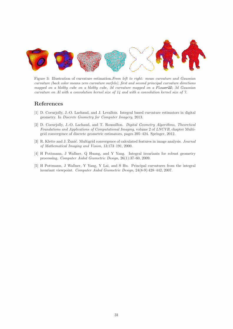
Figure 3: Illustration of curvature estimation.From left to right: mean curvature and Gaussiancurvature (back color means zero curvature surfels), first and second principal curvature directionsmapped on a blobby cube on a blobby cube, 2d curvature mapped on a Flower2D, 3d Gaussiancurvature on Al with a convolution kernel size of 14 and with a convolution kernel size of 7.
References
[1] D. Coeurjolly, J.-O. Lachaud, and J. Levallois. Integral based curvature estimators in digitalgeometry. In Discrete Geometry for Computer Imagery, 2013.
[2] D. Coeurjolly, J.-O. Lachaud, and T. Roussillon. Digital Geometry Algorithms, TheoreticalFoundations and Applications of Computational Imaging, volume 2 of LNCVB, chapter Multi-grid convergence of discrete geometric estimators, pages 395–424. Springer, 2012.
[3] R. Klette and J. Zunic. Multigrid convergence of calculated features in image analysis. Journalof Mathematical Imaging and Vision, 13:173–191, 2000.
[4] H Pottmann, J Wallner, Q Huang, and Y Yang. Integral invariants for robust geometryprocessing. Computer Aided Geometric Design, 26(1):37–60, 2009.
[5] H Pottmann, J Wallner, Y Yang, Y Lai, and S Hu. Principal curvatures from the integralinvariant viewpoint. Computer Aided Geometric Design, 24(8-9):428–442, 2007.
31

ISSN: 1885-4508