James Madison UniversityJMU Scholarly Commons

Masters Theses The Graduate School

Fall 2012

Implementation of signal conditioning circuitry forCO2 sensor for monitoring CO2 emissions fromcoal fired power plant in Neyveli LigniteCorporation (Tamil Nadu, India)Muruganand PrabhakaranJames Madison University

Follow this and additional works at: https://commons.lib.jmu.edu/master201019Part of the Environmental Sciences Commons

This Thesis is brought to you for free and open access by the The Graduate School at JMU Scholarly Commons. It has been accepted for inclusion inMasters Theses by an authorized administrator of JMU Scholarly Commons. For more information, please contact dc_admin@jmu.edu.

Recommended CitationPrabhakaran, Muruganand, "Implementation of signal conditioning circuitry for CO2 sensor for monitoring CO2 emissions from coalfired power plant in Neyveli Lignite Corporation (Tamil Nadu, India)" (2012). Masters Theses. 293.https://commons.lib.jmu.edu/master201019/293

1

IMPLEMENTATION OF SIGNAL CONDITIONING

CIRCUITRY FOR CO2 SENSOR FOR MONITORING CO2

EMISSIONS FROM COAL FIRED POWER PLANT IN

NEYVELI LIGNITE CORPORATION (TAMIL NADU, INDIA)

A dissertation presented in part fulfilment of the degree of

Master of Science in Sustainable Environmental Resource

Management/Master of Science in Integrated Science and

Technology.

Muruganand Prabhakaran

November 2012

Supervisor: Prof. Simon G. Fabri

University of Malta-James Madison University

2

ABSTRACT

MURUGANAND PRABHAKARAN

IMPLEMENTATION OF SIGNAL CIRCUITRY OF CO2 SENSOR FOR

MONITORING CO2 EMISSIONS FROM COAL FIRED POWER PLANT IN

NEYVELI LIGNITE CORPORATION (TAMIL NADU, INDIA)

The most significant anthropogenic greenhouse gas causing global warming is carbon dioxide

(CO2). Due to the increase of burning of fossil fuels by industries, the atmospheric CO2

concentration increased by more than 30% in 10 years and is expected to continue to increase.

This dissertation analyses a sensor unit used to monitor the emission levels of carbon dioxide

from the Neyveli Lignite Corporation (NLC) coal fired power plant which is located in the

southern part of India. Most of India’s power generation sectors are based on coal fired power

plants. The NLC power plant is owned by the central government of India. It can produce a

maximum electric power of 2490MW. The power plant lets out significant CO2 emissions while

generating electricity. These carbon dioxide emissions are the root cause for the greenhouse

effect. To control the carbon dioxide emissions, in this dissertation a sensor has been designed,

analysed and used to monitor the CO2 emission levels from the Neyveli Lignite Corporation.

This dissertation focuses on the design and implementation of the CO2 sensor using various

electronic components. In NLC, this CO2 sensor was kept under observation and tested. The

CO2 emissions measured by the sensor were analysed to monitor CO2 emissions from the

Neyveli Lignite Corporation and to guide measures and policy for future scenarios. This

dissertation identifies and examines the CO2 emission levels and the possible environmental

impacts. It also describes the advantages/disadvantages of the CO2 sensor and how this could

guide the possible reduction of greenhouse gases (GHGs) to meet a green environment agenda

in the future. Key environmental concerns in the coal-power sector in India include air pollution

(primarily from the flue gas emissions of particulates, carbon dioxide emissions, sulphur oxides,

nitrous and other hazardous chemicals) which has led to increased particulate pollution and ash

disposal problems. The enforcement of regulations to reduce CO2 emissions has been weak in

the southern part of India.

Key words: Carbon dioxide, Sensor, Greenhouse gases, Environmental, Impacts, Neyveli

Lignite Corporation

Supervisor: Prof. Simon G. Fabri MSc.SERM/MSc. ISAT

Co-Supervisor: Dr. Emil H. Salib November 2012

Reader: Dr. Jonathan Miles

3

The undersigned declare that this dissertation is based on work carried out under the auspices of

SERM/ISAT by the candidate as part fulfilment of the requirements of the degree of MSc.

Candidate Supervisor

This dissertation is dedicated to my mother who selflessly sacrificed her time with me so that I

could pursue my goals.

Special thanks is due first and foremost to my family for forever giving me undying support in

so many ways too numerous to articulate. I would also like to thank Prof. Simon G. Fabri for his

unreserved scrutiny and detailed analysis for being available when needed despite the eight hour

time difference, for his constructive analysis, and for his positive feedback.

4

Table of Contents

1. Chapter-1……………………………………………………………………………………………………………………….05

1.1 Introduction…………………………………………………………………………………………………….05

1.2 Background……………………………………………………………………………………………………..05

1.3 Environmental Concerns………………………………………………………………………………….06

1.4 Policy making…………………………………………………………………………………………………..07

1.5 Projected Future Demand………………………………………………………………………………..07

1.6 Objectives………………………………………………………………………………………………………..07

1.7 Structure of Dissertation………………………………………………………………………………....10

2. Chapter-2 Literature Review

2.1 Introduction……………………………………………………………………………………………………..11

2.2 Sensors in different fields………………………………………………………………………………...11

2.2.1 CO2 Chemical sensor…………………………………………………………….....11

2.2.1.1 Experimental Construction of Chemical Sensor…………………...11

2.2.2 Performance of the Sensor….......................................................12

2.2.3 Results and Discussion…………………………………………………………….13

2.2.3.1 Response Characteristics of the CO2 Sensor……………………………...13

2.2.3.2 Sensor Strategy for CO2 monitoring……………………………………..13

2.2.4 Monitoring of CO2 from space using remote sensing

Technique……………………………………………………………………………….14

2.2.4.1 Status CO2 and CH4 observing satellites…………………………………14

2.2.4.2 Atmospheric signature of power plant emission flumes……….14

2.2.5 CO2 Monitoring in Chemical Buildings……………………………………...16

2.2.5.1 Methodology………………………………………………………………………….17

2.2.5.2 Results……………………………………………………………………………………17

5

2.2.6 Assessing CO2 efflux with Solid state sensor…………………………………………18

2.2.6.1 Materials and Methods…………………………………………………………..19

2.2.6.2 Results and Discussions…………………………………………………………..19

2.3 Mitigation Strategies………………………………………………………………………………...19

2.4 CO2 metering device......................................................................................28

2.5 Designed CO2 sensor compared with other sensors.....................................28

3. Chapter-3 Components used to design signal conditioning circuitry of CO2 senor

3.1 Methodology....………………………………………………………………...........................20

3.2 Components used in the CO2 sensor Circuit……………………………………………..21

3.2.1 Gas Sensor…………………………………………………………………………………..21

3.2.2 PIC Microcontroller…………………………………………………………………….23

3.2.3 RS232 Serial Communication………………………………………………………38

3.2.4 Step-down Transformer………………………………………………………………43

3.2.5 Power Supply………………………………………………………………………………43

4. Chapter-4 Design and Implementation of signal circuitry circuit of CO2 sensor in NLC

4.1 Design of the Carbon dioxide sensor…………………………………………………………..45

4.2 Computer Aided Design……………………………………………………………………………...45

4.3 Printed Circuit Board Fabrication………………………………………………………………..46

4.4 Function of OrCAD layout in the PCB design process………………………………….47

4.5 Overview of the Design flow……………………………………………………………………….47

4.6 Complete design of CO2 sensor…………………………………………………………………..51

4.7 CO2 device kit (Software)..........…………………………………………………………………..54

4.8 CO2 sensor Calibration.....................................................................................61

6

5. Chapter-5 Monitored Report of Carbon dioxide emissions in Thermal Expansion II of NLC

5.1 Method of Estimation of Emissions………………………………………………………………56

5.2 Detailed Report of CO2 emissions from 2007 to 2011 in NLC………………………57

5.3 Monitored emissions of CO2 from the designed sensor………………………………57

5.4 Comparison between existing system and the proposed sensor………………….58

5.5 Implications.......................................................................................................68

6. Chapter 6- Results ……………………………………………………………………………………………………..71

7. Chapter 7- Policy Measures to control the Carbon dioxide emissions based on the data

publicly available from NLC ...................................................................……………………….76

7.1 Policies for Environmental Management……………………………………………………….76

7.2 Enabling Action……………………………………………………………………………………………...80

7.3 Advantages and Disadvantages……………………………………………………………………....81

7.4 Carbon tax……………………………………………………………………………………………………....82

8. Chapter 8-Conclusion & Future Work................................................................................81

Appendix I...............................................................................................................................85

Appendix II..............................................................................................................................91

7

Table of Figures

Figure 1: Neyveli Lignite Corporation

Figure 2: Coal Production in Neyveli Lignite Corporation

Figure 3: Projected Future Demand for Coal in India

Figure 4: Schematic structure and picture of the fabricated CO2 sensor designed by Ningliu

Figure 5: Schematic drawing of the experiment setup

Figure 6: CO2 concentration as a function of potential response (6.9Mpa)

Figure 7: Schwarze Pumpe satellite photo view

Figure 7: Simulated CO2 plume

Figure 8: CarbonSat orbital coverage for one day (21 June)

Figure 9: Measurement from 3 indoor locations

Figure 10: A schematic diagram of solid-state CO sensors

Figure 11: Carbon dioxide sinks-classification

Figure 12: Circuit diagram of MQ-2 gas sensor

Figure 13: 16-bit 28 pin PIC16F877A Microcontroller

Figure 14: Block Diagram of PIC16F877A

Figure 15: PIC16F877A Program Memory Stack

Figure 16: Block Diagram of PORTA RA30: RA pins

Figure 17: PORTC Block Diagram (Peripheral Output Over ride) RC<2.0>, RC<7.5>

Figure 18: PORTD Block Diagram (in I/O PORT Mode)

Figure 19: PORTE Block Diagram (In I/O PORT Mode)

Figure 20: PWM Output

Figure 21: Pin diagram of RS232 serial port to USB converter

Figure 22: Transmission of bytes in serial port

Figure 23: Simple null modem without handshaking

8

Figure 24: Turns ratio of 10:1 yields 10:1 primary: secondary voltage ratio and 1:10 primary:

secondary current ratio

Figure 25: Block Diagram of Power Supply

Figure 26: Circuit Diagram of Power Supply

Figure 27: Waveforms of Bridge rectifier

Figure 28: Double-sided copper clad FR4 substrate

Figure 29: Starting a new project in Capture

Figure 30: New project dialog box

Figure 31: Place Part dialog box

Figure 32: Add a library using browse file dialog box

Figure 33: Placing the parts in the Schematic diagram

Figure 34: Placing wires to connect the components

Figure 35: Complete circuit design of carbon dioxide sensor

Figure 36: CO2 metering device

Figure 37: Image view of complete PCB Carbon dioxide sensor

Figure 38: Column graph showing the variation of carbon dioxide emissions

Figure 39: Monitored carbon dioxide emissions using designed sensor

Figure 40: Electro static precipitator

9

Tables

Table 1: Estimates of extractable coal reserves in India

Table 2: Maximum CO2 column enhancement

Table 3: PIC 16F877A Device Features

Table 4: Special Function Registers RP1-RP0

Table 5: Summary of Registers associated with PORTA

Table 6: Summary of Registers associated with PORTB

Table 7: Summary of Registers associated with PORTC

Table 8: Summary of Registers associated with PORTD

Table 9: Summary of registers associated with PORTE

Table 10: CCP MODE-TIMER Resources Required

Table 11: Factors and units for calculating CO2 emissions

Table 12: Sector wise installed capacity in NLC

Table 13: Mass tons of CO2 emissions 2010-2011 in NLC

Table 14: CO2 emission report for the year 2007-2011 from NLC

Table 15: Monitored emissions of carbon dioxide from the designed sensor

Table 16: Reclamation Details in Mines of NLC

10

Acronyms

ADC- Analog to Digital Converter

AC –Alternating Current

ALU –Arithmetic Logic Unit

CAD-Computer Aided Design

CAE-Computer Aided Engineering

CCS-Carbon Capture and Storage

CFC-Chloro Fluro Carbon

Cm-Centi metre

CO2-Carbon dioxide

DC-Direct Current

DTE-Data Terminal Equipment

DCE-Data Communication Equipment

EIA-Environmental Impact Assessment

EEPROM-Electrically Erasable Programmable Read Only Memory

EPA-Environmental Protection Agency

F-Farad

FSR-File Select Register

GHG-Greenhouse Gas

GCV-Gas Calorific Value

I/O Port-Input/output Port

IGCC-Integrated Gasification Combined Cycle

IC-Integrated Circuit

IPCC-Intergovernmental Panel on Climate Change

KW-Kilo Watt

11

LCA-Life Cycle Analysis

mA-Milli Ampere

µF-Micro Farad

µmol-micro mole

MT-Mega Tonnes

MW-Mega Watt

MPa-Mega Pascal

mm-Milli metre

NCV-Net Calorific Value

NETL-National Energy Technology Laboratory

NLC-Neyveli Lignite Corporation

NOx-Nitrous Oxide

OCO-Orbiting Carbon Observatory

OrCAD-Oregon Computer Aided Design

PBL-Planetary Boundary Layer

PCB-Printed Circuit Board

PC-Pulverized Coal

PIC-Peripheral Interface Controller

Ppb-Parts per Billion

Ppm-Parts Per Million

PWM-Pulse Width modulation

RAM-Random Access Memory

ROM-Read Only Memory

RS232 Interface-Recommended Standard 232

R-Resistance

12

RL-Load Resistance

SO2-Sulfur dioxide

UART-Universal Asynchromous Receiver/Transmitter

USB-Universal Serial Bus

VT-Voltage Terminal

Vc-Loop Voltage

Vh-heater Voltage

VRl-Load Resistance Voltage

13

CHAPTER 1

1.1 Introduction:

The world’s fourth largest economy and one of the fastest growing energy markets is India. The

two major sources of energy are coal and petroleum. India’s main power generation sectors are

based on coal fired power plants [1]. Coal fired power plants are able to generate several Mega

Watts of electricity. Coal is a fossil fuel and approximately 62.3% of India’s electric power

generation is based on coal by National Thermal Power Corporation [1]. There are several coal

fired power plants in India for generating electricity and their amount has increased twice since

1967, due to rising population and changes in life styles, consistent with rapid economic

growths which have accelerated the energy demand [1].

This dissertation focuses on carbon dioxide emissions from the coal fired power plant called

Neyveli Lignite Corporation. In 1956, Neyveli Lignite Corporation was formed as a corporate

body. Neyveli Lignite Corporation is a government owned lignite mining and power generating

company in India. It has an installed capacity of 2740 MW and is presently mining 24 MT of

lignite. India’s carbon dioxide (CO2) emissions have been increasing at an average annual rate

of 5.5% from 1990 to 2000, with the coal accounting for about 70% of total fossil fuel

emissions [2]. The use of coal has some negative effects like environmental concerns, degraded

air quality and affects human health because of high particulates and sulphur dioxide emissions.

Emissions of carbon dioxide from the coal combustion power plant of NLC have been identified

as a primary culprit in increasing atmospheric CO2 concentrations, strongly affecting the

world’s climate [2]. NLC is mainly responsible for the current high CO2 atmospheric

concentrations in the southern part of India.

The need to reduce the CO2 emissions from India particularly in NLC has become an important

issue so, to control the emission levels this dissertation proposes a sensor which is used to

monitor the CO2 emission levels in Neyveli Lignite Corporation. NLC is at present using an

Orsat gas analyser, a piece of laboratory equipment used to analyse a gas sample (typically

fossil fuel flue gas) for its oxygen, carbon monoxide and carbon dioxide content. The use of this

type of instrument (Orsat flue gas analyzer) to analyse and monitor carbon dioxide emissions

will not give an efficient and accurate result. A flue gas analyzer is handheld instrument which

is not permanently installed near the thermal expansion II power plant. The use of this flue gas

analyzer is to analyse the combustible gases or smoke which comes out from the chimney of the

power plant. Being a hand-held instrument, flue gas analyser is not able to connect to digital

equipment because in NLC they are using analog instrument which is difficult to measure the

emission of combustible gases accurate as far as I observed in NLC power plant. Generally flue

gas analyzer is used when a probe is inserted into the flue of a boiler, furnace or other sources of

combustion to monitor the combustion gases. The Orsat gas analyzer is not efficient and

accurate because in NLC they use the analog instrument which is old method to measure the

combustible gases, which is a mixture of gases which has methane, nitrous oxide, sulfur oxide,

14

propane etc. So, it is difficult to diagnose which gas emits more and what their percentage

values.

Whereas, in the designed CO2 sensor the measurement process are reduced due to the placed

digital equipment. The truth is digital instruments are faster, more accurate, more reliable and

have a high repeatability than most analog tools. This is so because, in Orsat gas analyzer they

measure combustible mixture of gases but in designed CO2 sensor they measure only carbon

dioxide gases and it is easy to trace the carbon dioxide gas emissions by using this sensor. The

accuracy percentage of Orsat gas analyser is ±40 % but in designed carbon dioxide sensor the

accuracy is aimed to be about ±85 % [48]. While comparing the results of CO2 emissions with

designed sensor with flue gas analyzer, the emission reports are accurate due to their

performance and digital system(which includes microcontroller, ADC etc), repeatability,

reproducibility and robustness of the designed CO2 sensor.

The accuracy method used in Orsat gas analyzer is that the observed position peak on the analog

instrument indicates the time of retention and is characteristics of combustible gas component.

Retention time and sensitivity for each adsorbent material of combustible gases, aging and drift

are common so the Orsat gas analyzer is necessary to calibrate the instrument daily to obtain an

accuracy. Often, the Orsat gas analyzer cannot provide repeatable measurement for more than

400 ppm which clearly explains its inconsistency and reproducibility.

The term efficiency in the designed CO2 sensor explains that the sensor has its low power

consumption of 12 V Ac or DC supply, more precise in case of reproducibility, repeatability

and low cost compared to flue gas analyzer [49]. Why I say, the designed carbon dioxide is

more precise because the retention time for sensing the carbon dioxide gas in designed sensor is

less (micro seconds) which obtain its accuracy and also it can measure at the maximum level of

1000 ppm which tested in NLC power plant has its more amount of emissions nearly around

1000 ppm per hour. So to monitor specifically the carbon dioxide emissions from NLC, a CO2

sensor is designed using electronic components such as the PIC microcontroller, power supply

and serial communication because the use of PIC16F87A microcontroller has coded program,

serial communication has the transfer of each bit from one another and the use of 12 V power

supply will not consume more power compared to Orsat gas analyzer.

1.2 Background:

Widely considered as a major cause of climate change, greenhouse gases (GHGs) permit

sunlight to move through the earth’s atmosphere. The heat radiated from Earth’s surface is

absorbed by the GHGs and re-radiated back to Earth, effectively trapping the heat in the

atmosphere. CO2 contributes the most significant gas compared to all amount of GHG

emissions [3].

It is well known that India is the third –largest producer of coal in the world and that Indian

coal is of poor quality with 35-50% of high ash content and low calorific value (gross heat of

15

combustion) [1]. The demand for coal in India’s power plants has rapidly increased since the

1970s with power plants in 2005-2006 absorbing about 80% of the coal produced in the country

[3]. It is to be noted that the combustion of fuels from furnace oil and natural gas have

decreased by 32.55% since 1998-2000 [1]. Eventually, this led to a high increase of combustion

of lignite coal by 7.54%.

The main emissions from coal combustion at Neyveli Lignite Corporation are carbon dioxide

(CO), nitrogen oxides (NO), sulphur oxides (SO), chlorofluorocarbons (CFCs) and other

inorganic particles [1]. One should note that CO2 produced in combustion is perhaps strictly not

a pollutant but acts as a base indicator for global warming [2].

The estimates of extractable coal reserves in India are shown in table 1:

Table 1: Estimates of extractable coal reserves in India

Source: Chand, Ministry of Coal [2].

There are several block units in Neyveli Lignite Corporation which have several mines that

generate Kilo watts of power and that can be supplied to several districts in Tamil Nadu. So, by

generating electricity, these mines produce high emissions of CO2.

Depending upon the rate of domestic coal production, coal use in NLC might last anywhere

from 30 to 60 years. This threatens that there might be a lot of coal production from NLC which

will cause atmospheric CO2 emissions if the emission rate still continues for this time-period.

The expected coal production rate in NLC is 1020 MW in further years and the carbon dioxide

gas emission level right now in NLC is 20 Mega tonnes and is expected to increase up to 50

Mega tonnes.

1.3 Environmental Concerns

NLC is a coal based power plant that significantly had an impact on environmental concerns by

emitting carbon dioxide and also flue gases from ash coal to the atmosphere [4]. There are some

direct impacts to the environment from NLC that include:

Production of hazardous chemicals

16

Creates pollution near local streams, rivers and contaminating ground water from

effluent discharges

Degradation of land that is used for storing fly ash

Air pollution and also basic indicator for GHG emissions [4]

Indirect impacts of these coal fired power plants includes degradation and destruction of land,

deforestation, displacement, resettlement and rehabilitation of people affected, who work near

the mining regions [4].

Figure 1: Neyveli Lignite Corporation

Source: Neyveli Lignite Corporation Limited- Tamil Nadu [3]

Figure 1 shows the environment in and around region of the Neyveli Lignite Corporation. These

chimneys emit flue gas which has the mixture of concentrations of SO2, CO2 and particulate

matters.

1.4 Policy Making:

The monitoring results of the CO2 sensor being proposed in this dissertation, for use in the NLC

may be analysed and processed by governmental agencies in order to take some necessary

measurable actions and policies to control the emission levels from NLC. Better energy

planning and policies would require a good understanding of domestic coal reserves in NLC

like, the coal reserves of any particular place are defined as the amount of measured resource

coal that could be expected to be economically mineable under the current economical and

technological conditions and it is important to reduce existing uncertainties like more amount of

17

carbon dioxide emissions in NLC power plant by implementing suitable policy making to

obtain green environment(zero emissions).

Figure 2: Coal Production in Neyveli Lignite Corporation: Hard Coal production excludes

lignite production

Source: The coal data is from Ministry of Coal Annual reports (1999-00, 2003-04, 2005-06,

2006-07). Data for lignite is from MOSPL [5].

Figure 2 shows the production of coal in NLC since 1960. Continuing with its dominant role in

the commercial energy spectrum of the country, the All-India (including NLC-Tamilnadu) Coal

production improved to 432.062 Mt in 2006-07 from 362 Mt in 2002-03, thus it grew by 8%

over the last year [5].

Neyveli Lignite Corporation extracts coal using the method of underground mining, which is

used to extract very deep coal seams. It also involves constructing a vertical shaft or slope mine

entry to the coal seam and then extracting the coal using long wall techniques (Ward, 1984).

This increases the production level of coal in NLC and subsequently also increases the

atmospheric CO2 emission levels.

The government has also received several suggestions regarding coal consumption and the

control of CO2 emissions in the Neyveli Lignite Corporation. The committee of Environmental

Protection Agency in NLC has recommended the creation of an office of the Coal Governance

and Regulation Authority with the five directorates:

Coal Resource Management

Safety, Health and Employment

Prices, Taxes, Royalty, Value Added Tax, Property Tax and Salary of Workers

18

Environmental Management

Cap and Trade Mechanism

Policy-Legal, Public Participations, Statistics and Dispute Resolution

1.5 Projected Future Demand

In short, coal is projected to be the main resource for power generation in India, despite

projected increases in natural gas, nuclear and renewable energy in the country (section on

Future Growth and Continued Reliance on Coal). Since, coal is a non-renewable resource it is

expected to rise in the demand for the production of electricity [5].

The demand projection of coal and lignite in NLC is expected to be about 480MT by 2013.

Because of the demand projection and supply shortages some plants in the NLC have pulled

back on generation and have partially shut down under critically low coal stock levels.

Figure 3: Projected Future Demand for Coal in India

Source: Planning Commission of India [5].

Figure 3 shows the coal vision 2025 with the Environmental Impact Assessment high and low

levels. In India, coal is the major source for electricity and because of the rise in population, the

amount of coal used has increased. Being a non- renewable resource, coal has short life span.

As more Indians enjoy the trappings of middle-class life and the country industrialises, demand

for coal-fired electricity will continue to rise, roughly in line with economic growth. If this case

extends in India, there might be a rise of demand in electricity and coal production.

1.6 Objectives of this project

The objectives of this project on Design and Implementation of CO2 Sensor include the

following

19

Design of a low cost signal conditioning circuit of CO2 sensor using off-the-shelf and

standard electronic sub-systems like the PIC Microcontroller, ORCAD and Serial

Communications

Monitor the CO2 emission levels (Tonnes) using the designed signal conditioning

circuit of designed CO2 sensor in the NLC power plant

An analysis of the measured CO2 emissions

Compare results between the existing CO2 sensing method in NLC and the

proposed CO2 sensor results

Suggestion of policy for Emission Regulation and Clean Environment

Suggest some future work in the designed carbon dioxide sensor for better

efficiency.

1.7 Structure of dissertation

According to the research plan, the dissertation is divided in to the following chapters where

Chapter 2 will give the overview of the Literature Review and focuses on how various methods

have been handled to monitor and control the CO2 emissions

Chapter 3 explores the methodology of the design of the CO2 sensor using various electronic

components and also analyse the block diagrams of various components

Chapter 4 investigates the implementation of the CO2 sensor in the Neyveli Lignite Corporation

and their implications of the circuit.

Chapter 5 extracts the monitored report of the CO2 emissions in the NLC and also compares the

result with the existing and proposed system.

Chapter 6 merges the results of the final report with various stages of monitored CO2 emissions

Chapter 7 discusses policy measures that can be used to control carbon dioxide emissions

Finally chapter 8 wraps up the thesis and suggests ways how this project could move forward in

future research.

20

CHAPTER 2 -LITERATURE REVIEW

2.1 Introduction

Sensors and sensor networks have an important impact in meeting the environmental

challenges. Sensors have been discussed in detail within selected fields of application that have

a high potential to reduce greenhouse gas emissions and review studies quantifying

environmental impact.

This chapter will seek to provide an overview of different sensors used to monitor atmospheric

emissions. Primarily section 2.2 briefly identifies the design and use of sensors in the

environment to control CO2 emissions and also explains how such sensors work to monitor

atmospheric emissions. Section 2.3 clearly explains the mitigation strategies for carbon dioxide

emissions and their improvement in energy efficiency by adapting different methods.

2.2 Sensors in different fields

Sensors have been used in different fields of environment to determine the concentration levels

of chemicals in the atmosphere.

2.2.1 CO2 Chemical Sensor

Mc Pherson et al., [6] describe downhole CO2 chemical sensor to determine the concentration

of CO2 in water, particularly in harsh, high pressure environments. This sensor is tested under a

pressure of 6.9Megapascal in the geological area. These sensors have been used in many fields

[6].

2.2.1.1 Experimental construction of the CO2 Chemical Sensor

Nowadays, concentration of CO2 levels in the atmosphere increases due to anthropogenic

causes. To reduce the CO2 emission levels and also to store the carbon dioxide, geological

sequestration of CO2 has been proposed to store the large amounts of carbon dioxide in

underground formation. This sensor was designed to resist harsh environmental conditions such

as high pressure and high ionic strength. Miura et al., [45] also reported that the CO2 sensor

might work at high pressure, but the disadvantage of his sensor is that it cannot work in high

humidity when CO2 is dissolved in water [6].

This sensor has been prepared for the detection of CO2 underground with a Severinghaus-type

pair of electrodes, a gas permeable membrane; a bi-carbonate based internal electrolyte solution

and some support materials as shown in the figure 4.

21

Figure 4: Schematic structure and picture of the fabricated CO2 sensor designed by Ningliu.

Source: Chemical Sensor Journal [6].

2.2.2 Performance of the Sensor

The value of the CO2 sensor output was measured by a potentiometric 34401A 61/2 digital

multimeter [45]. The CO2 concentration can be calculated from the added amount of

NaHCO3solution. The schematic drawing of the experiment setup of the CO2 sensor is shown

in figure 5.

Figure 5: Schematic drawing of the experiment setup

Source: Agricultural and Forest Metrology [6].

22

2.2.3 Results and Discussions

2.2.3.1 Response characteristics of the CO2 sensor

With respect to the direction of the concentration change of CO2, the response time of the

sensor was found to be dependent on the concentration. For higher level of CO2 concentration,

the average response time was around one hour while a little slower response time was observed

at low concentration range [6]. The electrodes placed inside the experimental setup of the

sensor, records the response time of the sensor with the considerable levels of CO2

concentration.

2.2.3.2 Sensor Strategy for CO2 monitoring

The concentration of CO2 is monitored in the underground at different sites such as injection

wells, observation wells, shallow water wells and green-fields to detect the possible CO2

leakage.

Thus, all the acquired data from the sensor will automatically transmit to the well surface using

the wireless network. These data were collected and stored in the computer for the future

analysis [6].

2.2.4 Monitoring of CO2 from space using remote sensing technique

The author [7] describes how CO2 concentration in space is monitored using existing satellite

instruments such as SCIAMACHY/ENVISAT and TANSO/GOSAT. A remote sensing unit is

designed based on spectroscopic measurements of reflected solar radiation where the localized

CO2 point sources can be detected and their emissions quantified. Each power plant is

monitored from space using a single satellite in sun-synchronous orbit with a swath width of

500Km for every 6 days or more frequently [7].

It has already been recognized that global satellite observations of the CO2 vertical column (in

molecules/cm2) or of the CO2 dry air column-averaged mole fraction (in ppm), denoted XCO2,

has the potential to significantly advance our knowledge of regional natural CO2 surface

sources and sinks provided the satellite measurements have significantly high sensitivity to the

planetary boundary layer (PBL), where the source/sink signal is largest, and are precise and

accurate enough [7].

2.2.4.1 Status CO2 and CH4 observing satellites

In 2002, the first satellite instrument called SCIAMACHY/ENVISAT using short-wave infrared

was used to detect CO2 variations of a few parts per million [7].

2.2.4.2 Atmospheric signature of power plant emission plumes

23

A quasi-stationary Gaussian plume model is used to simulate the CO2 vertical column

enhancement of a simulated CO2 plume at high spatial resolution and at a distance of 2*2

square kilo meter corresponding to the resolution of the Carbon-Sat satellite instrument

discussed with the detailed figure 7 below [7].

Figure 7: Schwarze Pumpe satellite photo view (left) Figure 7: Simulated CO2 plume

Figure 7 (left) depicts the atmospheric CO2 column enhancement due to CO2 emission of a

power plant location which is indicated by the black cross mark. The green colour which has the

value of 1 corresponds to the CO2 column. The red colour which has the value of 1.02

corresponds to a column enhancement of 2% to the CO2 emissions.

The assumed power plant emission which is shown in figure 7 is 13MtCO2/yr corresponding to

a power plant such as Schwarze Pumpe located in eastern Germany near Berlin.

Horizontal resolution Peak of CO2 column

normalised to background (-)

20m*20m 1.126

40m*40m 1.125

1Km*1Km 1.053

2Km*2Km 1.031

4Km*4Km 1.017

10Km*10Km 1.005

Table 2: Maximum CO2 column enhancement

24

Table 2 above depicts the maximum CO2 enhancement (relative to back-ground column =1.0)

for a power plant emitting 13MtCO2/yr for different spatial resolutions of the satellite footprint.

The assumed wind speed in space is 1m/s.

Figure 8: CarbonSat orbital coverage for one day (21 June)

Source: H. Bovensmann et al., Monitoring CO2 emissions from Space [7].

Figure 8 shows about the satellite CarbonSat orbital coverage measured in one day (21 June) for

a swath width of 500 km corresponding to 250 across-track ground pixels of width 2km each.

The coverage shown in the green depicts the main mode called nadir mode over land and the

coverage shown in the blue depicts the sun-glint mode over water [7].

2.2.5 CO2 Monitoring in Commercial Buildings

Carbon dioxide sensors are designed to obtain CO2 data in commercial buildings for demand-

controlled ventilation. This type of demand controlled ventilation is most often used in spaces

with highly variable and sometime dense occupancy. The study in [8] entailed (a) locating 208

CO2 single-location sensors in 34 commercial buildings (b) Four multiple locations of CO2

measurement that utilize tubing, valves and pumps to measure multiple locations with single

CO2 sensors and also the spatial variability of CO2 concentrations within meeting rooms. The

sensor monitors CO2 concentration in indoor and outdoor unit environment and if the indoor

CO2 concentration in an office work environment is 700 parts per million above the outdoor

concentration, the ventilation rate is approximately set to 7.5 L/s (15cfm) per person.

Epidemiological research has found that indoor CO2 concentrations are useful in predicting

human health and performance [8].

2.2.5.1 Methodology

A single location CO2 sensor was designed under the method of two phases. The sensor

analyses the data from both study phases, with the total of 208 sensors which is located in 34

buildings. This kind of method is called multi-concentration calibration check.

25

Figure 9: Measurement from 3 indoor locations

Source: Indoor Environmental Quality Research [8].

Figure 9 shows a schematic representation of one of three systems employed to rapidly measure

indoor carbon dioxide concentrations at three indoor locations per system. These three systems

were placed to monitor the indoor carbon dioxide concentration on each wall at approximately

1.50m above the floor.

2.2.5.2 Results of CO2 monitoring in Commercial Buildings

To estimate the CO2 monitoring results of this study, one must get the required accuracy of CO2

sensors used in commercial buildings for demand controlled ventilation. The difference between

indoor and outdoor CO2 concentration is a better indicator of building ventilation rate because

outdoor concentrations of CO2 vary significantly with the time and locality. This puts pressure

on the design of the sensor because one needs to be able to determine with reasonable accuracy

the difference between the peak indoor and outdoor concentrations of CO2 found in commercial

buildings [8].

2.2.6 Assessing CO2 efflux with small solid-state sensors

The author describes a new method to monitor continuously CO2 concentrations in the soil

continuously using small solid-state sensors buried at different depths of the soil. The soil CO2

efflux was determined from heterotrophic respiration in the soil using a solid-state sensor in a

Mediterranean savanna ecosystem in California [9].

2.2.6.1 Materials and methods

There are different methods that have been applied to monitor underground CO2 concentrations

in the soil.

26

Soils

The oak-grass savanna has a rocky silt loam type of soil called Auburn. The soil is normally

composed of 48% of sand, 42% of silt and 10% of clay which is about 0.75 m deep with a bulk

density.

Environmental measurements

Environmental measurements like relative humidity, air temperature and static pressure were

measured using their respective sensors and the volumetric soil moisture is monitored

continuously in the field using domain reflectometry sensors (Theta Probe model ML2-X,

Delta-T Devices, Cambridge, UK). These sensors were sampled at every second and half-hour

averages were computed and stored on a computer. These measurements were compared with

the flux measurements.

Figure 10: A schematic diagram of solid-state CO2 sensors

Source: Tang et al, Agricultural and Forest Meteorology [9].

Figure 10 represents the encased probes buried in the soil at three depths with transmitters for

receiving the signals which is then send to a data logger. These data were stored in Computer

memory for future reference [9].

2.2.6.2 Results and Discussions

The results found in [9] using small solid-state sensors are

The daily mean average values of CO2 did not vary significantly at a depth of 2 cm, but the

value decreases slightly at a depth of 8 and 16 cm. The daily mean CO2 concentration varied

between 386 and 403 µmol mol‾1 with an average over 36 days of 396 µmol mol‾1.

Volumetric moisture of the soil at the depth of 5 cm had no significant diurnal variation, and it

decreased slightly from 6.5 to 5.9% with an average of 6.3% over the 36 day drying period.

27

The soil has more carbon dioxide concentrations which causes the diurnal variations in the

atmosphere like climatic changes. The results found using the solid state sensors indicates that

green house gas emissions are due to the deposition of carbon dioxide sensor in the soil. The

solid state sensor has the probe similar to the designed carbon dioxide sensor used to monitor

the CO2 emissions in the atmosphere.

2.3 Mitigation strategies

Besides monitoring CO2 emissions using sensors, some mitigation strategies like increasing

sinks, reduction of carbon dioxide sources, afforestation, fuel mix, improvement in energy

efficiency, replacement of fossil fuels for power generation with renewable or nuclear energy

sources and carbon sequestration should be considered [10].

2.3.1 Supply side options for mitigation of CO2 emissions

Mitigation of CO2 emissions from the supply side are mainly classified as efficiency

improvements on existing generating plants, advanced cleaner technologies and renewable

energy based power plants.

2.3.2 Carbon dioxide sinks

Disposal of carbon dioxide in to sinks can help to mitigate CO2 levels. The best of such

mitigation options include biosphere sinks (oceans, forest, vegetation and soils), geosphere

sinks and sequestration (oil reserves, coal beds, depleted oil and gas reservoirs, deep ocean and

deep aquifers) and material sinks (durable wood products, chemicals and plastics [8], as shown

in figure 11.

Figure 11: Carbon dioxide sinks-classification

Source: U.S Department of Energy [2].

Reduction measures can be improved further by using low amounts of carbon fuels and efficient

systems for power generation, and also enhancing the growth of sinks.

28

It is to be noted that CO2 emissions cannot be reduced within a short span of time, because the

achievement of clean coal technologies, renewable energy sources and sinks also take their own

time to reduce CO2 in the atmosphere [10].

2.4 CO2 metering device

CO2 metering device is user friendly software which is used to convert the values ppm

concentrated values into Metric tons. This software is designed with the sensor design where it

can be installed in every computer if the user has its own sensor circuit design. This sensor

circuit is designed in which CO2 Meter's own in-house developed, fully-featured data

acquisition package. It is used to store the real time data which was sensed by the sensor. Here,

it is interesting that this sensor metering software does not require any components to design,

just to store the sensed values from the sensor for future reference. But compared this software

with designed carbon dioxide sensor, the designed sensor has several electronic components

with more efficiency, accuracy up to 80 % and it has more applications like compact, easy to

install, hardware components and low cost compared to the metering device [47].

2.5 Designed sensor compared with other sensors

By comparing the designed carbon dioxide sensor with the above mentioned sensor circuits like

satellite sensing method sensor is more expensive design and it cannot afford by NLC to use or

purchase this type of sensor. The CO2 chemical sensor which is already mentioned is used to

sense the carbon dioxide gas in the geological area with high pressure and high ionic strength

and moreover it cannot work in high humidity when CO2 is dissolved in water. This kind of

sensor cannot use by NLC because for NLC the main objective is to monitor the gas emissions

from chimney which is in the thermal expansion II power plant. But this sensor senses only the

underground gases and more over cannot work when CO2 dissolved in water so this sensor

cannot sense the emissions when there is heavy rain in and around NLC regions. The other

sensor which mentioned is CO2 monitoring in commercial buildings. This sensor is used to

monitor the carbon dioxide gas in door and out door units of commercial buildings. Moreover,

the response time will be low and it cannot sense the high amount of emissions like 1000 ppm

concentration. Moreover, the accuracy, repeatability will be less because if this sensor operates

for more than 2 days continuously then there will be decrease in its sensitivity.

The above mentioned sensors are highly expensive and it is not easy grade to purchase and

install but the designed sensor has more accuracy in terms of its response time. It has its

response time of less microseconds and it can measure more number of values within one hour.

It can detect upto 10000 ppm and there will not decrease in their sensitivity if it continues to

sense prolong for more than 10 days continuously. I can say that NLC use this designed carbon

dioxide sensor because of its low cost, detect high concentrated values, easy to install, less

power consumption and need not to replace often once installed.

29

CHAPTER 3- Components used to design signal conditioning circuit of CO2 sensor

3.1Methodology

Carbon dioxide sensing has an important impact in meeting environmental challenges. Sensor

technology plays an important role for green growth. Because of the important impact of

applications of sensors and sensor networks in meeting environmental challenges, the signal

conditioning circuit of carbon dioxide sensor proposed in this dissertation has been developed

using standard electronic components like the MQ series semiconductor gas sensor (CO2 gas

sensor) [11] which senses the CO2 gases, the PIC microcontroller, serial communications (RS

232 interface), serial port, and a standard power supply. With these components, the design of

signal conditioning circuitry of carbon dioxide sensor is designed to monitor the carbon dioxide

gas emissions in Neyveli Lignite Corporation.

The tool used to design the CO2 sensor circuitry is the OrCad capture and layout software.

Computer-aided design (CAD) is a category of computer-aided engineering (CAE) that is

related to the physical layout and drawing development of a system design. Once a design has

been proven through drawings, simulations and analysis, the system (sensor) can be

manufactured [18].

3.2Components used in the CO2 sensor circuit

The components used in the design of the carbon dioxide sensor circuit are the MQ series

semiconductor gas sensor (CO2 sensor), a PIC microcontroller, an RS 232 interface serial port,

a step down transformer and a power supply.

3.2.1Gas sensor

The MQ-2 semiconductor sensor has a sensitive material SnO2. It has its lower conductivity in

clean air. In the presence of the target combustible gas (release of carbon dioxide from the

power plant), the sensor’s conductivity goes higher along with the gas concentration. The circuit

of the sensor converts the conductivity to a corresponding output voltage representing gas

concentration. The circuit has the loop voltage Vc is less than 24V DC, heater voltage VH

5.0V±0.2 V AC or DC. The output concentration of the combustible gas will be 300-10000 ppm

and their corresponding voltage will be 20V to 25 V DC [11].

The MQ-2 gas sensor has high sensitivity to Carbon dioxide gas which is designed exclusively

to sense the carbon dioxide gases. The MQ2 sensor I have used in this circuit is sensitive to

carbon dioxide gases only not to whole range of gases which is shown in data sheet in appendix

I. It has with low cost and is suitable for different applications [11].

30

Circuit diagram

Figure 12: Circuit diagram of MQ-2 gas sensor

Source: MQ-2 Data Sheet [11].

Figure 12 is the basic test circuit of the sensor. The sensor requires 2 voltage supplies, heater

voltage (VH= 5.0 V±0.2V AC or DC) and test voltage (VC≤ 24 V DC). VH is used to supply the

certified working temperature to the sensor, while VC is used to detect voltage (VRL) on load

resistance (RL) which is in series with the sensor. VC needs DC power, so the power is supplied

form the 230 volt DC power supply. VC and VH could use the same power circuit with

preconditioning to assure performance of sensor [11]. Refer to the appendix for MQ-2 Sensor

specifications.

Characteristics of sensor

Good sensitivity to carbon dioxide gas in wide range which is quantitatively more sensitive

Long life which has its life span of 4 to 5 years

Low cost (25 USD) compared to other sensors like humidity and temperature sensor

Simple driver circuit

Application

Domestic gas leakage detector

Industrial combustible gas detector

Portable gas detector

Notification for MQ-2 gas sensor

The following conditions should be prohibited while using this sensor:

MQ-2 series sensor must avoid exposure to silicon bond, fixature, silicon latex and plastic

containing silicon environment. To handle this constraint, sensor should not keep in indoor

conditions, slight water condensation to avoid the exposure.

31

Sensor should not be exposed to high concentration corrosive gas such as H2Sz, SOx, Cl2, HCl

etc because sensor’s sensitivity to sense carbon dioxide gas gets decreased.

The alkali metals salt should not be polluted on the sensors, because the sensor performance

will be changed badly.

The applied voltage should not exceed the stipulated value, otherwise it can cause system error

or heater damage and the sensors sensitivity characteristic can be changed badly [11].

3.2.2 PIC Microcontroller

A PIC microcontroller is a processor which includes memory and RAM and can be used for

control projects. A PIC microcontroller is a very powerful device that has many useful built in

modules used to save complex circuits like external RAM, ROM and peripherals chips.

The PIC microcontroller used in this device is PIC 16F877A which comes from the family of

PIC 16F87XA. PIC16F877A devices are available in 44 pin packages as shown in the figure 13.

It has the following features

The total on-chip memory of the PIC16F877A has more than one half of that PIC16F873A and

PIC16F874A.

It has five I/O ports with 44 pin devices.

It has fifteen interrupts and eight A/D input channels.

Figure 13: 16-bit 28 pin PIC16F877A Microcontroller

Source: Microchip-PIC Microcontroller 16F877A Data sheet [12]

32

The PIC16F877A device features are explained in table 3

Key Features PIC 16F877A

Operating Frequency DC- 20 MHz

Resets (and Delays) POR, BOR (PWRT, OST)

Flash Program Memory (14 bit words) 8K

Data Memory (bytes) 368

EEPROM Data Memory (bytes) 256

Interrupts 15

I/O ports Ports A,B,C,D,E

Timers 3

Capture/Compare/PWM modules 2

Serial Communications MSSP, USART

Parallel Communications PSP

10 bit Analog to Digital Module 8 input channels

Analog Comparators 2

Instruction set 35 instructions

Packages 40 pin PDIP

44 pin PLCC

44 pin TQFP

44 pin QFN

Table 3: PIC 16F877A Device Features

Block Diagram of PIC 16F877A

Figure 14: Block Diagram of PIC16F877A

Source: U.S Microchip Technology [12].

33

Figure 14 represents the block diagram of the PIC microcontroller. The device parameters are

explained below

Memory organization:

There are three memory blocks in the PIC16F877A device. The separate buses are program

memory and data memory. It has its own concurrent access as shown in figure 15. It has several

data bytes with the on-chip program memory and it is interconnected to each other with the

interrupt vector.

Figure 15: PIC16F877A Program Memory Stack

Source: U.S Microchip technology [12].

Data memory organization:

The PIC16F877A has its data memory portioned into multiple banks which contain the General

purpose Registers and the Special Function Registers. The bank select bits comprise the bits

RP1 (Status<6>) and RP0 (Status<5>) as shown in table 4.

34

RP1-RP0 Bank

00 0

01 1

10 2

11 3

Table 4: Special Function Registers RP1-RP0

General Purpose Register:

Either directly or in directly through the File Select Register (FSR), the register file can be

accessed. The lower locations of each bank are reserved for the Special Function Registers as

shown in table 4. Above the Special Function Registers are General Purpose Registers,

implemented as Static RAM in the PIC microcontroller [12].

Status Register:

The arithmetic status of the ALU, the reset status and the blank select bits for data memory have

portioned in the Status Register. It can be used for any instruction with any other register. If the

Status Register has the destination for an instruction, which affects Z, DC or C bits, then these

three bits are disabled. These bits are set or cleared according to the device logic.

R/W-0 R/W- 0 R/W-0 R-1 R-1 R/W-x R/W-x R/W-x

IRP

RP1

RPO

‾‾‾‾

TO

‾‾‾‾

PD

Z

DC

C

bit 7 bit 0

bit 7 IRP: Register Bank Select bit(used for indirect addressing)

1= Bank 2, 3 (100h-1FFh)

0= Bank 0, 1 (00h-FFh)

bit 6-5 RP1:RP0: Register bank Select bits (used for direct addressing)

11= Bank 3 (180h-1FFh)

10= Bank 2 (100h-17Fh)

01= Bank 1 (80h-FFh)

00= Bank 0 (00h-7Fh)

Each bank is 128 bytes.

bit 4 TO: Time –out bit

35

1= After power-up, CLRWDT instruction or SLEEP instruction

0= A WDT time out occurred

bit 3 PD: Power-down bit

1= After power-up or by the CLRWDT instruction

0= By execution of the SLEEP instruction

bit 2 Z: Zero bit

1= The result of an arithmetic or logic operation is zero

0= The result of an arithmetic or logic operation is not zero

bit 1 DC: Digit carry/borrow bit (ADDWF, ADDLW, SUBLW, SUBWF instructions)

1= A carry-out from the 4th

low order bit of the result occurred

0= No carry-out from the 4th

low order bit of the result

Bit 0 C: Carry/borrow bit (ADDWF. ADDLW, SUBLW, SUBWF instructions)

1= A carry-out from the Most Significant bit of the result occurred

0= No carry-out from the Most Significant bit of the result occurred

I/O Ports

An input/output port in the device is represented by I/O ports. For peripheral feature on the

device, I/O ports are multiplexed with an alternate function. In general, when a peripheral is

enabled, that pin may not be used as a general purpose I/O pin.

The different types of I/O ports present are

PORTA and the TRISA Register

PORTB and the TRISB Register

PORTC and the TRISC Register

PORTD and the TRISD Register

PORTE and the TRISE Register

36

PORTA and the TRISA Register

A bidirectional port with 6 bit wide and their corresponding data direction register TRISA is

PORTA. By setting a TRISA bit (=1) will make the corresponding PORTA pin an input (i.e.,

put the corresponding output driver in a High-Impedance mode). PORTA is initialised by

coding the following program

BCF STATUS, RP0 ; BCF STATUS, RP1 ; Bank0 CLRF PORTA ; Initialise PORTA by clearing output ; data latches BSF STATUS, RP0 ; Select Bank 1 MOVLW 0*06 ; Configure all pins MOVWF ADCON1 ; as digital inputs value used to initialise data direction MOVWF TRISA ; set RA<3:0> as inputs ; RA<5:4> as outputs ; TRISA<7:6> are always ; read as “0”

Figure 16: Block Diagram of PORTA RA30: RA pins

Figure 16 represents the arrangements of blocks in the PORTA I/O pins and their output is

internally connected to the Analog to Digital converter. PORTA register is used to read the

status of the pins, whereas writing to it will write to the port latch. The block diagram shows the

Data bus, Schmitt Trigger, TRISA and the A/D converter. Pin RA4is multiplexed with the

Timer0 module clock input to become the RA4/TOCKI pin. The RA4/TOCKI pin is a Schmitt

Trigger input and an open-drain output [12].

37

Other PORTA pins are multiplexed with analog inputs and the analog VREF input for both the

A/D converters and the comparators. When TRISA register is used as analog input, it controls

the direction of the port pins. The user must ensure that bits in the TRISA register are

maintained set when using them as analog inputs.

Table 5: Summary of Registers associated with PORTA

Table 5 shows the summary of registers associated with PORTA and when using the module

PORTA, the PORTA of bit 3 to bit 0 should be adjusted to the PCFG3: PCFG0=0100, 0101,

011x, 1101, 1110, 1111 respectively.

PORTB and the TRISB Register

A bidirectional port with an 8 bit wide and their corresponding data direction register TRISB is

PORTB. Setting a TRISB bit (=1) will make the corresponding PORTB pin an input. Clearing a

TRISB bit (=0) will make the corresponding PORTB pin an output. Three pins of PORTB are

multiplexed with the In-Circuit debugger and the Low-Voltage programming function.

Table 6: Summary of Registers associated with PORTB

Table 6 shows the summary of registers associated with PORTB and the cells like TOCS,

TOSE, PSA, PS2, PS1 and PS0 are not used by PORTB.

PORTC and the TRISC Register

A bidirectional port with an 8 bit wide and their corresponding data direction TRISB is PORTC.

PORTC is multiplexed with several peripherals functions (Table7). PORTC pins have Schmitt

Trigger input buffer. To enable each peripheral function, care should be taken in defining TRIS

bits for an each PORTC pin. Some peripherals in the PORTC over ride the TRIS bit to make a

pin an output, while other peripherals over ride the TRIS bit to make a pin an input.

38

Figure 17: PORTC Block Diagram (Peripheral Output Over ride) RC<2.0>, RC<7.5>

Table 7: Summary of Registers associated with PORTC

Table 7 shows the summary of registers associated with PORTC which represents x as an

unknown and u as unchanged.

PORTD and TRSID Register

To be noted that PORTD and TRISD are not implemented on the 28 pin devices. PORTD is an

8-bit port with Schmitt Trigger input buffers as shown in the figure 18. Each pin is individually

configurable as an input buffers. Each pin is individually configurable as an input or output.

PORTD can be configured as an 8-bit wide microprocessor port (Parallel Slave Port) by setting

control bit, PSPMODE (TRISE<4>). In this mode, the input buffers are TTL.

Figure 18: PORTD Block Diagram (in I/O PORT Mode)

39

Table 8: Summary of Registers associated with PORTD

Table 8 shows the summary of registers associated with PORTD with the x as unknown, u as

unchanged and the bits 3, 2, 1 and 0 are not used by PORTD.

PORTE and TRISE Register

PORTE has three pins (RE0/RD/AN5, RE1/WR/AN6 and RE2/CS/AN7) in the below block

diagram which are individually configurable as inputs or outputs. These pins have Schmitt

Trigger input buffers.

The PORTE pins become the I/O control inputs for the microprocessor port when bit

PSPMODE (TRISE<4>) is set. In this mode, the user must make certain that TRISE<2:0> bits

are set and that the pins are configured as digital inputs. Also that ADCON1 is configured for

digital I/O port.

Figure 19: PORTE Block Diagram (In I/O PORT Mode)

Figure 19, explains that the Register 4-1 shows the TRISE register which also controls the

Parallel Slave Port operation. When selected for analog input, these pins will read as ‘0’s and

they are multiplexed. The direction of the RE pins are controlled by the TRISE when they are

being used as analog inputs. The user must make sure to keep the pins configured as inputs

when using them as analog inputs.

40

Table 9: Summary of registers associated with PORTE

Table 9 shows the summary of registers associated with PORTE with x as unknown, u as

unchanged and the bits 7, 6, 5, 4, 3 are read as 0 and not used by PORTE.

TIMER0 MODULE

The Timer0 module in the PIC microcontroller (timer/counter) has the following features:

8-bit timer/counter

Readable and writable

8-bit software programmable prescaler

Internal or external clock select

Interrupt on overflow from FFh to 00h

Edge select for external clock

CAPTURE/COMPARE/PWM Modules

Each capture/compare/PWM (CCP) module contains a 16-bit register which can operate as a

16- bit capture register

16-bit compare register

PWM Master/Slave Duty cycle register

Both Capture and Compare modes are identical in operation.

CCP Mode Timer Resource

Capture Timer 1

Compare Timer 1

PWM Timer 2

Table 10: CCP MODE-TIMER Resources Required

41

Capture Mode

In Capture mode, CCPR1H: CCPRL captures the 16-bit value of the TMR1 register when an

event occurs on pin RC2/CCP1. This event is defined as one of the following

Every falling edge

Every rising edge

Every 4th

rising edge

Every 16th

rising edge

This type of event is configured by control bits CCP1M3:CCP1M0. When a capture is made,

the interrupt request flag bit, CCP1/F is set.

Compare Mode

In Compare mode, the 16-bit CCPR1 register value is constantly compared against the TMR1

register pair value. When a match occurs between two registers, pin is:

Driven high

Driven low

Remains unchanged

The action on the pin is based on the value of control bits CCP1M3:CCP1M0. At the same time,

interrupt flag bit CCP1F is set. To initiate the action, an internal hardware trigger is generated.

The special event trigger output is used (CCP1) which resets the TMR1 register pair. This

allows the CCPR1 register to effectively be 16 bit programmable periods register for Timer 1.

The special event trigger output (CCP2) which resets the TMR1 register pair and starts an A/D

conversion (if A/D conversion is enabled) [12].

Pulse Width Modulation Mode

In Pulse Width Modulation mode, the CCPx pin produces up to a 10-bit resolution PWM

output. Since, the CCP1 pin is multiplexed with the PORTC data latch, the TRISC<2> bit must

be cleared to make the CCP1 pin output.

The PWM period is specified by writing to the PR2 register. The PWM period can be calculated

using the following formula

PWM period= [(PR2) +1]*4*TOSC*(TMR2 Pre-scale Value) [13].

PWM frequency is defined as 1/ [PWM Period]

42

When TMR2 is equal to PR2, the following three events occur on the next incremental cycle:

TMR2 is cleared

The CCP1pin is set (exception: if PWM duty cycle=0% the CCP1 pin will not be set)

The PWM duty cycle is latched from CCPR1L into CCPR1H as shown in the figure 20.

Figure 20: PWM Output

Source: Arduino, chip technology [13].

It is to be noted that the PWM duty cycle value is longer than the PWM period, the CCP1 pin

will not be cleared.

Code Space

The coding for the PIC microcontroller is generally implemented as ROM, EPROM or flash

ROM. The other PIC microcontrollers external code memory is not directly addressable due to

the lack of an external memory interface expect for the PIC16F877A microcontroller.

Software emulation in the PIC microcontroller is done by the method called debugging. In this

PIC16F877A microcontroller, coding is built in the chip to communicate with this interface

using three lines.

By following this coding, the microcontroller can be used with the MPLAB IDE for the full

source-level debugging of the code running on the target. The entire action in the

microcontroller follows the coding and performs the action.

#include<pic.h> #include<stdio.h> #include"delay.c" __CONFIG(0x3f71); float MQ2; int CO2gas,CO2gas1;

43

void GetMQ2(void); void Serial_init(void); void main() { Serial_init(); TRISA=0xff; ADCON1=0x00; DelayMs(10); while(1) { GetMQ2(); printf("CO2 GAS VALUE:%f \r",MQ2); DelayMs(250); DelayMs(250); } } void MQ2() { ADCON0=0x41; DelayMs(1); ADGO=1; while(ADGO==1); CO2 gas=ADRESH; ADRESL=ADRESL>>6; CO2gas=CO2gas<<2; CO2gas=CO2gas+ADRESL; MQ2=CO2 gas value*100/204.9; } void Serial_init() { TRISC=0xc0; TXSTA=0x24; SPBRG=25; RCSTA=0x90; TXIF=1; } void putch(unsigned char data) { while(TXIF==0); TXREG=data;

44

}

The ADC conversion value is 1023 ADC Levels/5V = 204.6 ADC Levels / Volt

ADC_CONVERSION_FACTOR 204.6

The Analog to digital conversion value from PIC microcontroller is 1023 which is in four bits

divided by the respective voltage of the PIC microcontroller which is 5 volts. It is divided to

know the actual value of the conversion factor in analog to digital converter.

Analog to Digital converter

The Analog to digital converter is an integrated circuit in the PIC16F877A microcontroller. It is

used to convert the analog signal which is sensed by the sensor into a digital representation.

The perfect example of analog to digital conversion is when we record our voice on computer;

voice is converted into digital and transmitted by the computer using ISDN or DSL over the

network.

The purpose of using the digital conversion is to reduce the noise which is interpreted as being

part of the original signal. Another advantage of a digital signal is the data compression

capability, where analog signals which have a high range can be compressed into less size [12].

The compression can be done to save storage space or bandwidth so that data will be used for

future reference.

Advantages of PIC Microcontroller

The advantages of PIC microcontroller are

Small instruction set to learn

RISC architecture

Built in oscillator with selectable speeds

Easy entry level, in circuit programming in circuit debugging

3.2.3 RS232 Serial Communication

Serial Communication is basically defined as the transmission or reception of data one bit at a

time. A byte contains 8 bits and is basically either a logical 1 or 0. The serial port is used in this

circuit to convert each byte to a stream of ones and zeroes and vice versa. The serial port

contains an electronic chip called a Universal Asynchronous Receiver/Transmitter (UART) that

actually does the conversion as shown in the figure 21.

45

Figure 21: Pin diagram of RS232 serial port to USB converter

Source: Raptor, Elektor electronics [14]

Transmitter and Receiver pin:

The serial port has many pins, but transmitter and receiver play a vital role in the serial of

transmitting and receiving the data. When no data is being sent, the serial port’s transmit pin

voltage is negative (1) and is said to be in a MARK state. Note that the serial port can also be

forced to keep the transmit pin at a positive voltage (0) and is said to be the SPACE or BREAK

state [14].

Figure 22: transmission of bytes in serial port

Source: Parallax Inc [14].

Figure 22 shows how a byte transmission would look like in a serial port. When transmitting a

byte, the UART (serial port) first sends a START BIT which is positive voltage (0), followed

by the data (generally 8 bits, but could be 5, 6, 7 or 8 bits) followed by one or two STOP BITs

which is negative (1) voltage. The sequence is repeated for each byte sent.

46

Serial communication can be half duplex or full duplex.

Half Duplex Serial Communication Full Duplex Serial Communication

A device cannot send and receive at the

same time

Device can receive and transmit data at the

same time

It is outdated except for a very small focussed

set of applications

Full duplex is a updated device

Needs minimum two wires, signal ground and

the data line

Needs minimum three wires, signal ground,

transmit data line and receive data line.

These signals are the Carrier Detect Signal (CD), Ring Indicator (RI), Data Set Ready (DSR),

Clear to Send (CTS), Data Terminal Ready (DTR), Request to Send (RTS).

For further control of the information flow, both devices (DTR & DTE) have the ability to

signal their status to the other side. For this purpose, the DTR data terminal ready and DSR data

set ready signals are present. The DTE uses the DTR signal to signal that it is ready to accept

information, whereas the DCE uses the DSR signal for the same purpose. Using these signals

involves not a small protocol of requesting and answering as with the RTS/CTS handshaking.

These signals are in one direction only [14-15].

Null modem without handshaking

The simplest way to use the handshaking lines in a null modem configuration is not to use them.

In that situation, only the data lines and signal ground are cross connected in the null modem

communication cable. All other pins have no connection. An example of null modem cable

without handshaking can be seen in figure 23.

Figure 23: Simple null modem without handshaking

Connector 1 Connector 2 Function

2 3 T

3 2 T

5 5 Signal ground

47

Compatibility Issues

If we read about null modems, this three wire null modem cable is easy to use in all

circumstances. There is a problem, if either of the two devices checks DSR or CD inputs. These

signals are normally define the ability of the other side to communicate. If they are not

connected, their signal level will never go high. This might cause a problem [15].

Advantages of Serial port (RS232)

The advantages of Serial port (RS232) are as follows:

With stands high temperature

Operate with single 5V power supply

Operate up to 120kbit/sec

Two Drivers and Two Receivers

±30V Input levels

Low supply current…8mA typical one

Designed to be interchangeable with Maxim max232

Applications

TIA/EIA-232-F

Battery Powered Systems

Terminals

Modems

Computers

3.2.4 Step-down Transformer

In this circuit, a step down transformer is used to decrease the voltage from the power supply,

which is then fed in to the PIC microcontroller. The Step down transformer coils were made of

identical inductance, giving approximately equal voltage and current between primary and

secondary windings of the transformer.

48

Figure 24: Turns ratio of 10:1 yields 10:1 primary: secondary voltage ratio and 1:10 primary:

secondary current ratio

Source: Circuits, Volume II-AC Transformers [16].

Figure 24 illustrates, how the secondary voltage is approximately ten times less than the

primary voltage (0.9962 volts compared to 10 volts), whereas the secondary current is

approximately ten times greater (0.9962 mA compared to 0.09975 [16].

3.2.5 Power Supply

The power supply is a device that supplies electrical power to an electrical load. The power

supply is connected to the circuit through the step down transformer. The AC voltage typically

220V RMS is connected to a transformer, which steps that AC voltage down to the level of the

desired DC output [17].

Figure 25: Block Diagram of Power Supply

Figure 25 represents the block diagram of the power supply. It has the transformer which is

connected to the rectifier, the output of the rectifier is connected to the filter to reduce the noise,

the output of the filter is connected to the IC regulator and then finally it is connected to the

load.

A diode rectifier provides a full-wave rectified voltage that is initially filtered by a simple

capacitor filter to produce a DC voltage. A regulator circuit removes the ripples and also

remains the same DC value even if the input DC voltage varies, or the load connected to the

output DC voltage changes. This voltage regulation is usually obtained using one of the popular

voltage regulator IC units as shown in figure 26.

TRANSFORMER RECTIFIER FILTER IC REGULATOR LOAD

49

Figure 26: Circuit Diagram of Power Supply

Source: John Hewes, The Electronics Club[17].

Working Principle

Transformer

The potential transformer will step down the power supply voltage (0-230V) to (0-6V) level.

Then the secondary of the potential transformer will be connected to the precision rectifier. The

advantages of using precision rectifier in this circuit is it will give peak voltage output as DC

voltage, rest of the circuits will give only RMS output.

Bridge rectifier

The four diodes are connected in the circuit as shown above is called bridge rectifier. The input

to the circuit is applied to the diagonally opposite corners of the network, and the output is taken

from the remaining two corners.

50

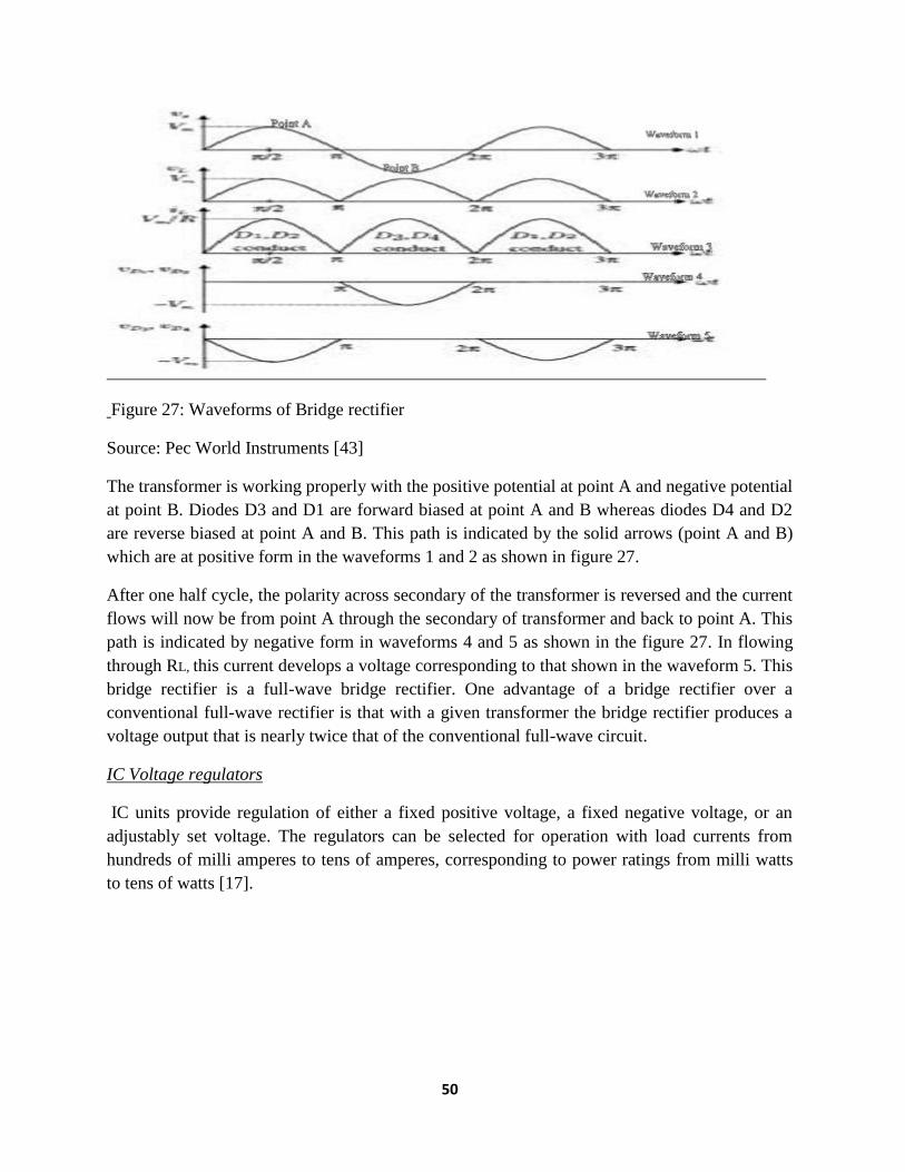
Figure 27: Waveforms of Bridge rectifier

Source: Pec World Instruments [43]

The transformer is working properly with the positive potential at point A and negative potential

at point B. Diodes D3 and D1 are forward biased at point A and B whereas diodes D4 and D2

are reverse biased at point A and B. This path is indicated by the solid arrows (point A and B)

which are at positive form in the waveforms 1 and 2 as shown in figure 27.

After one half cycle, the polarity across secondary of the transformer is reversed and the current

flows will now be from point A through the secondary of transformer and back to point A. This

path is indicated by negative form in waveforms 4 and 5 as shown in the figure 27. In flowing

through RL, this current develops a voltage corresponding to that shown in the waveform 5. This

bridge rectifier is a full-wave bridge rectifier. One advantage of a bridge rectifier over a

conventional full-wave rectifier is that with a given transformer the bridge rectifier produces a

voltage output that is nearly twice that of the conventional full-wave circuit.

IC Voltage regulators

IC units provide regulation of either a fixed positive voltage, a fixed negative voltage, or an

adjustably set voltage. The regulators can be selected for operation with load currents from

hundreds of milli amperes to tens of amperes, corresponding to power ratings from milli watts

to tens of watts [17].

51

CHAPTER 4: Design and Implementation of signal circuitry of CO2 Sensor in Neyveli

Lignite Corporation in Thermal Expansion II power plant

4.1 Design of the Carbon dioxide Sensor

The complete design of Carbon dioxide sensor is made using Computer-Aided Design and the

OrCAD design suite.

4.2 Computer Aided Design

CAD covers all aspects of engineering design from drawings to analysis to manufacturing. CAD

is a category of CAE that is related to the physical layout and drawing development of a system

design. CAD programs are specific to electronic design automation called ECAD. It reduces the

development time and cost of the circuit. A design has been proven through drawings,

simulations and analysis, the system can be manufactured [18].

4.3 Printed Circuit Board Fabrication

PCB refers to”Printed Circuit Board” which consists of two basic parts: a substrate (the board)

and the printed wires (the copper traces). A structure which physically holds the circuit

components and printed wires in place with electrical insulation between conductive parts are

called substrate. A common type of substrate is FR4, which is fibre-glass-epoxy laminate. It is a

flame resistant and substrates are made from Teflon, ceramics and special polymers.

During manufacturing, the PCB starts out as a copper clad substrate as shown in figure 28. The

copper cladding may be copper that is plated onto the substrate or copper foil that is glued to the

substrate.

Figure 28: Double-sided copper clad FR4 substrate

Source: Kraig Mitzner, Elsevier’s Science and Technology [18]

52

PCB fabrication process

On a PCB one can see the copper traces and pads. It is produced by selectively removing the

copper cladding and foil. The two common methods for removing the unwanted copper are wet

acid etching and mechanical milling.

Acid etching

It is a more common method while manufacturing large quantities of boards because the

advantage is that many boards can be made simultaneously. One disadvantage of this method is

that chemicals are hazardous and must be replenished occasionally, and the depleted chemicals

must be recycled or discarded.

Mechanical milling

Milling is used for smaller production runs and prototype boards. During milling, the traces and

pads are formed by a rotating bit that grinds the unwanted copper from the substrate [18].

4.4 Function of OrCAD layout in the PCB Design process

By generating a digital description of the board layers, the layout is designed and is used to

manufacture the boards. There are separate layers for routing copper traces on the top, bottom

and all inner layers; drill holes sizes and locations; solder masks; silk screens; solder paste; part

placement and board dimensions. Some of the layers mentioned above are shown from the

positive prospective, meaning the layers are placed on the board with the OrCAD software

whereas, negative perspective represents that the OrCAD software remove layers from the

board.

The layers represented in the positive view are the board outlines, routed copper, silk screens,

solder paste and assembly instructions. The layers represented in the negative view are copper

plane layers, drill holes and solder masks.

Design files created by layout

Layout format files (.MAX)

When designing the board with layout works, layout design format is to be saved in the

computer. The layout design file has a MAX extension. After all process, is ready to fabricate

the board, layout post processes the design and converts it into format that photo-plotters and

CNC machines can use. These files are called Gerber files.

Post-process (Gerber) files

Post processing creates a separate Gerber file for each of the layers. There can be as many as 30

or so different layer files that layout generate to describe various manufacturing aspects of PCB.

53

Now that we have covered the construction of a PCB we will go to overall design process.

4.5 Overview of the Design flow

The overview of design flow illustrates the basic procedure for generating a schematic in

capture and converting the schematic to a board design in layout. The basic procedure is as

follows:

Start capture and set up a PCB project using the PCB project using the PC board wizard

Make a circuit schematic using OrCAD capture

Use Capture to generate a layout net list and save it as a .MNL file for layout

Start layout and select a PCB technology template (.TCH file)

Save the layout project as a .MAX project file

Use layout to import the .MNL net list into .MAX file

Make a board outline

Position the parts within the board outline

Autoroute the board

Run the post-processor to generate files used to manufacture the PCB.

Creating a circuit design with capture

To set up a PCB project, first we have to create the circuit with capture and the following

procedures:

Starting a new project

First, a circuit layout is designed to make PCB layout by capture, so the first step is to start the

capture application by clicking windows Start button on the task bar and navigate to ALL

Programs-> OrCAD 10.5 Demo-> Capture CIS Demo. Then we can create a new project and

save it as shown in figure 29.

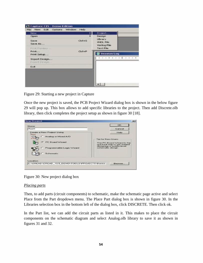
54

Figure 29: Starting a new project in Capture

Once the new project is saved, the PCB Project Wizard dialog box is shown in the below figure

29 will pop up. This box allows to add specific libraries to the project. Then add Discrete.olb

library, then click completes the project setup as shown in figure 30 [18].

Figure 30: New project dialog box

Placing parts

Then, to add parts (circuit components) to schematic, make the schematic page active and select

Place from the Part dropdown menu. The Place Part dialog box is shown in figure 30. In the

Libraries selection box in the bottom left of the dialog box, click DISCRETE. Then click ok.

In the Part list, we can add the circuit parts as listed in it. This makes to place the circuit

components on the schematic diagram and select Analog.olb library to save it as shown in

figures 31 and 32.

55

Figure 31: Place Part dialog box

Figure 32: Add a library using browse file dialog box

By placing the different components of the circuit, select Normal in the graphic list and add

value to the parts. For example, if a capacitor is added, the value of the capacitor in micro farad

should be noted. The same procedure is done for all the components of the circuit that are

placed in the schematic diagram as shown in figure 33.

56

Figure 33: Placing the parts in the Schematic diagram

Wiring (connecting the parts)

After placing the parts in the schematic diagram, insert the wires to be connected between the

parts to make a complete circuit. To place the wires, hit the W key, or select Place-> Wire from

the Place dropdown menu. Place the cursor on a box at the end of the one of the part’s leads and

left click to start a wire connection as shown in figure 34. Click on the part of the circuit to

complete that wire. Once circuit wired connection is finished, press the ESC key or right click

and select End Wire to stop the place wire cursor and the pointer back.

Figure 34: Placing wires to connect the components

By using this software, these procedures are followed by placing different components of the

circuit and wired up. This makes the complete circuit of the carbon dioxide sensor and the

circuit layout is printed using PCB. After all these procedures, the components are placed on the

PCB and soldered using the made connections.

57

4.6 Complete design of Carbon dioxide Sensor:

Figure 35 represents the complete design of the carbon dioxide sensor circuit.

Figure 35: Complete circuit design of carbon dioxide sensor

Figure 35 shows the complete design of the signal conditioning circuit of the designed carbon

dioxide sensor which was designed by me by referring some of the sensor circuits and altered

some changes in the circuit by adding microcontroller, serial communication etc [48]. The code

which debugged into the microcontroller for collecting CO2 gas data are as follows

VCC

VCC_BAR

MCLR

C3

10uF

Y1

4 Mhz

C7

CAP

PIC16F877A

123456789

10

11

12

1314

15161718

1920

4039383736353433

32

31

30292827

26252423 22

21

MCLR/VPPRA0/ANORA1/AN1RA2/AN2/VREF-/CVREFRA3/AN3/VREF+RA4/TOCKI/C1OUTRA5/AN4/SS/C2OUTREO/RD/AN5RE1/WR/AN6RE2/CS/AN7

VD

D

VS

S

OSC1/CLKIOSC2/CLKO

RCO/T1OSO/T1CKIRC1/T1OSI/CCP2RC2/CCP1RC3/SCK/SCL

RD0/PSP0RD1/PSP1

RB7/PGDRB6/PGC

RB5RB4

RB3/PGMRB2RB1

RB0/INT

VD

D

VS

S

RD7/PSP7RD6/PSP6RD5/PSP5RD4/PSP4

RC7/RX/DTRC6/TX/CKRC5/SDORC4/SDI/SDA RD3/PSP3

RD2/PSP2

R3

330E

C5

470uF

/25V

C1

10uF

C5470uF

/25V

SW0

RST

U1

MAX232

138

1110

1

3

4

5

2

6

129

147

16

15

R1INR2IN

T1INT2IN

C+

C1-

C2+

C2-

V+

V-

R1OUTR2OUT

T1OUTT2OUTV

CC

GN

D

C3

10uF

P1

SE

RIA

L P

OR

T

594837261

C3

10uF

Gas Sensor

123

58

void main()

{

unsigned int adc_value;

float ppm_value;

TRISE.B0=1; // RE5 as input

Computer display_Init();

ADC_Init();

while(1)

{

Get the current ADC value (PIC Microcontroller)

Read the ADC for the latest value

adc_value = ADC_Read(5);

Convert the ADC value to the PPM concentration

ppm_value = ADC_TO_PPM_CONVERSION_FACTOR*adc_value;

}

//Display the ppm value on the computer display

Computer_display(1,1,ppm value);

strcpy("PPM:", computer_display);

delay_ms(1000);

}

The coding explains how the MQ2 series sensor senses the carbon dioxide gases and converts it

into voltages which are in the analog value. These analog value voltages are then converted into

digital bits by ADC which actually does the conversion by PIC microcontroller. While coding

the program in the PIC microcontroller this ADC to PPM conversion command is encoded, this

displays the converted analog digital value in to ppm concentration which it actually does. This

conversion factor is explained in the below example how the ADC reads the digital bit and its

59

real voltage which is converted into ppm value. The loop follows each and every value and

converts digital bits to ppm value. These ppm values are then stored in the computer display

which is converted into Metric tons by using ppm conversion software.

For example The ADC LEVEL to PPM conversion factor is 1000PPM/1023ADC LEVELS =

0.9775

#define ADC_TO_PPM_CONVERSION_FACTOR 0.9775

If the ADC reads 512(digital bit), the real voltage is 2.5 VDC and the PPM level is 500PPM.

This is just an example (an assumption) I stated how the analog to digital conversion factor is

used to change the digital bits into ppm values. Here if ADC output reads 512 digital bits and

then the real voltage measured in the sensor is 2.5 voltage so the ppm conversion value will be

500 ppm.

4.7 CO2 device kit

Figure 36: CO2 metering device [47]

CO2 metering device kit is user friendly software which is commercially available and easy to

download in windows XP can be used to convert the ppm values into Metric tons or vice versa.

This software also does several other conversions which can view the data in real time or

manage stored data with internal memory. Once the sensor design was completed, this software

is installed in the computer to view ppm conversion results into Metric tons on the computer

display [47]. This software displays the carbon dioxide gas emission data in the ppm

concentration. These values are stored for future reference. This is actually software I haven’t

used for circuit design. This software was downloaded to convert the ppm values into required

Metric tons value.

60

Working principle

The design of the CO2 sensor is intended to analyse and monitor the emissions of CO2 from coal

burning power plants. By installing this sensor in the coal burning power plant (NLC), the rate

of emissions of CO2 every 5 hours is calculated. This makes the staff of NLC power plant aware

to control the emissions of CO2 and also the effects on the environment. Monitoring of CO2

emissions from NLC can be done in 2 ways. Either by connecting the required components such

as temperature, humidity and also carbon dioxide sensors, with a purposely designed board that

has a fast time response and low power consumption with tolerance against moisture, and acts

as a perfect solution for greenhouse environment. The second way of monitoring carbon dioxide

emissions is just by utilizing the existing flue gas analyser which detects combustible gases

from the power plant. My project focuses on the former circuit design to monitor the emission

level from the power plant, the Neyveli Lignite Corporation.

This sensor is placed near the chimney of the Thermal Expansion II of the Neyveli Lignite

Corporation. The Thermal Expansion II of the NLC power plant operates under 250 MW of

energy production. Once the sensor senses the carbon dioxide gas, the switch terminal

connected to the microcontroller closes the circuit and this analog value of the carbon dioxide

gas is recorded in the microcontroller. The microcontroller includes an analog to digital

converter that converts this analog voltage into a digital value. Beside the microcontroller, two

capacitors are placed in parallel with a piezo crystal Y1 to act as a crystal oscillator as shown in

the figure 34. The microcontroller has the transmission and receiver end which transmits and

receives the value of the carbon dioxide gas. The receiver end is connected to the input of the

RS232 interface. Once the value is converted into the digital unit, it is transmitted to the RS232

interface. The interface converts each byte of the signal to the corresponding one’s and zero’s of

the digital unit. The RS232 interface stores the value of the digital output. The transmission and

receiver output pin is connected to the input of the serial port. This serial port is then connected

to the USB port converter via the computer. Once the signal is converted into digital signal and

its value stored in the RS232 interface, it is then transmitted to the computer through the USB

port converter. Once the values have been noted, it is stored in standard file format. These

values of CO2 emissions can be stored for future reference. The values are noted in ppm (parts

per million). The concentration of carbon dioxide emissions are always calculated in ppm

concentrations.

61

Figure 37: Image view of complete PCB Carbon dioxide sensor

Figure 37 shows the complete designed carbon dioxide sensor which has several components

such as the sensor, PIC microcontroller, step-down transformer, USB converter and RS232

serial interface. The laptop is placed beside the circuit to store the values of emissions from the

power plant. The laptop is connected to the RS232 interface of the circuit through the USB port

converter.

4.8 CO2 Gas sensor Calibration

Sensors need to be calibrated before implementation to ensure sensor accuracy and system

integrity. The whole circuit of the sensor is calibrated by the manufacturer once the instrument

is designed but it is always good practice to check the sensor before installation to identify

sensitivity, influence of sensor location, influence of other gases etc. The way to calibrate the

sensor circuit is “span” calibration. It is a complicated and e pensive method to calibrate the

sensor. This is done by sensing the mixture of target gas balanced in the background

environmental air which is the best calibration gas. The most preferred method to calibrate the

sensor circuit is premixed gas mixtures. To calibrate the sensor in this method, the needed

components are regulator assembly, pressure gauge and the orifice flow restrictor. The working

principle of this method is that the orifice flow restrictor is fitted in the outlet of the sensor with

a hairline hole that allows a constant air flow at a high pressure difference. This pressure was

indicated in the pressure regulator and the pressure is constantly increased by adjusting the

pressure gauge. This how the sensor circuit should be calibrated. After calibration, the sensor

circuit, sensor should be monitored for first 30 days in room conditions to sense the carbon

62

dioxide gases for testing and confirm that it works properly before implementing it in NLC.

This method of calibration provides good degree of confidence about the implementation of

sensor. I acknowledge that I don’t have enough time to test the designed sensor for 30 days

because NLC (government owned sector) gave permission to monitor the carbon dioxide gas

from thermal expansion II just for 6 days. Moreover, to calibrate the sensor, calibration

instruments like calibration gas, regulator, flow meter, dryer tube or wetting material is needed.

These procedures should be done in certified laboratory and moreover I designed this carbon

dioxide sensor in my house, it will not be convenient to calibrate the sensor. If these instruments

were available, I would have calibrated the designed sensor under span method as mentioned

earlier by adjusting the flow rates of the gas and the pressure difference using pressure gauge.

To calibrate this CO2 sensor, setting the “Zero” reading method is done where the established

standard for this sensor is zero. It is more realistic to zero the sensor using clean surrounding air

in an area that is considered to be clean. The use of pure nitrogen or synthetic air to establish the

zero point is readily available. This sensor was calibrated under pure air to give a clear

representation of the zero point which mostly applies to much solid state sensor instrumentation

but the zero reading method using pure nitrogen or pure synthetic air is not so effective and

correct to calibrate the designed sensor. This is so because; the ambient air which considers the

pure air contains normally small percentage of water vapour. So, this zero reading method for

calibration is not enough to the designed carbon dioxide sensor.

63

Chapter-5 Monitored Report of Carbon Dioxide emissions in Thermal Expansion II of

NLC

Carbon dioxide emissions from the Thermal Expansion II of the Neyveli Lignite Corporation

were monitored for seven hours for the period of three days using the designed CO2 sensor and

their values compared with the previous CO2 emissions report of NLC.

Carbon dioxide emissions are conventionally estimated based on the consumption of fuel (coal)

in the thermal power plant II of NLC. The more rate of consumption of coal indicates a high

generation of electricity and more carbon dioxide emissions. So, high generation of electricity is

directly proportional to the high rate of emissions of carbon dioxide gases [20].

Deforestation is also a major source of carbon dioxide emission due to the increase in

population and growth of industries [21]. The Neyveli Lignite Corporation thermal power plant

has the most influence of carbon dioxide emissions in Tamil Nadu in India due to improper

maintenance of the chimney. In addition, the placement of scrubbers in the power plant is not

proper. The change of scrubber should be performed every 6 months according to the

Environmental Protection Agency.

5.1 Method of Estimation of Emissions

The estimation of carbon dioxide emissions from the NLC power plant is based on the amount

of coal consumed to generate 250 MW of electricity. Coal is the major source for the NLC

power plant to generate electricity. Nearly 250 Mega Watts of electricity are generated from the

NLC and being supplied to many states in Southern India.

The methods [22] were used to estimate the amount of CO2 emitted to the atmosphere from the

fossil fuel burning in the Neyveli Lignite Corporation. This method is very simple to use and

easy to understand how to calculate the emissions from the power plant. For each type of fuel,

the annual CO2 emissions are the product of three terms: the amount of fuel consumed in the

power plant, the fraction of the fuel that is oxidized and a factor for the carbon content of the

fuel [22].

In this dissertation, the fuel used for the electricity generation is coal, so the three terms that

need to be considered are the amount of coal consumed for the generation of electricity in the

power plant, the fraction of coal that is oxidized and the factor for the carbon content of the coal

according to the following equation.

CO2c= (Pc) (FOc) (Cc)

Where suffix c represents the use of a particular fuel.

Pc represents the amount of fuel c that is consumed each year

64

FOc is the fraction of Pc that is oxidized

Cc is the average carbon content for the fuel and

CO2c is the resulting CO2 emissions for fuel c expressed in mass of carbon [22].

Factors and units for calculating CO2 emissions from fuel consumption

The factors and units for calculating CO2 emissions from the NLC are based on the

consumption of the coal for generation of electricity. It is calculated with the used metric tons of

carbon, annual production and consumption rate of coal (fuel) and their amount of carbon

content in the fuel [21] as shown in Table 11.

From primary and secondary solid fuel (coal) production and consumption trade in NLC

CO2c = CO2 emissions in 10^6 metric tons of carbon

Pc = annual production or consumption in 10^6 tons coal equivalent

FOc = 0.982± 2%

Cs = Carbon content in tons C per ton coal equivalent = 0.746 ± 2%

Table 11: Factors and units for calculating CO2 emissions

Source: Marland and Rotty[22].

5.2 Detailed Report of CO2 emissions from 2007 to 2011 in NLC

The energy data for the carbon dioxide emissions from the Thermal Expansion II of the Neyveli

Lignite Corporation have been compiled by the Centre for Monitoring Emissions (CME). CME

is located in Tamil Nadu, India [49]. It provides a long time series data on the production and

consumption of coal for electricity generation in NLC and also their carbon dioxide emissions

in a yearly manner as a complete form of report. The estimation of carbon dioxide emissions are

based on the coal consumption. The details of the data sources and the type of fuel (coal) and

their carbon dioxide emissions are furnished

Using the data base of the Neyveli Lignite Corporation with CME, calculation of baseline

carbon dioxide emission factors depends upon the consumption of coal for electricity generation

and the installed capacity of Thermal Power plant. As a result of the impressive growth attained

by the Indian power sector, the installed capacity of NLC has grown from mere 1,713 MW in

1965 to 15939 MW as on 31.10.2010, consisting of 5,782 MW in Thermal Expansion I, 6,895

MW in Thermal Expansion II and the rest in Thermal Expansion III [24]. This is shown in table

12.

Sector Capacity

Thermal Expansion I 5782 MW

Thermal Expansion II 6895 MW

Thermal Expansion III 3262 MW

Total 15939 MW

65

Table 12: Sector wise installed capacity in NLC

5.3 Monitored emission of CO2 from the designed sensor

In this work, the carbon dioxide sensor is designed to monitor the emission levels in the Neyveli

Lignite Corporation in Tamil Nadu, India. The designed sensor was installed in the NLC power

plant near the chimney of the Thermal Expansion II, where lots of emissions in NLC were

reported by Tamil Nadu government in India [29] The emissions are in the form of combustible

gases that includes sulfur dioxide, nitrous oxide, methane and carbon dioxide. This designed

sensor sensed only the carbon dioxide gases which are the root cause for green house gases. The

designed carbon dioxide sensor was tested to sense the other gases like methane and Chloro-

fluro carbons which emits from the air conditioning unit but found that it doesn’t sense these

gases. The designed sensor is kept under observation for two hours near the place where several

air conditioning units are installed. I’m not sure whether they released large amounts of CFC

were emitted. This how I tested the designed sensor whether it is sensing the CFC gases or not.

If designed sensor senses the carbon dioxide gases, then there will be blinking of LED light

which is placed in the designed sensor. This understands me that there is a emission of carbon

dioxide gases from this region. But for testing CFC gases, there is no blink in the LED indicates

that it doesn’t sense the CFC gas. The sensor has monitored the emission gases for seven hours

a day within a period of three days in the months of June and July 2012. These reports have

been analyzed and the average emissions of carbon dioxide were furnished below.

CO2 emissions of thermal power station (NLC) were calculated using the formula below:

AbsCO2 (thermal station II)y = ∑ Fuel Con i,y * GCV i,y * EF I * Oxid I

Where:

AbsCO2 y Absolute CO2 emission of the Thermal expansion II station

Fuel Con i,y Amount of fuel of type I consumed

GCV i,y Gross calorific value of the fuel

EFi CO2 emission factor

Oxidi Oxidation factor of the fuel [26].

The emission and oxidation factors used in the CO2 database are provided in Appendix II.

This is the method (formula) used by the NLC monitoring station to analyse the emission levels

of combustible gases from thermal expansion II by Orsat gas analyzer.

The operating margin of absolute CO2 emission values is calculated as the generation-weighted

average CO2 emissions per unit net electricity generation (tCO2/MWh) of thermal expansion II

66

of NLC power plant. Fuel consumption and GCV are generally not measured at unit level,

instead the specific CO2 emissions of the relevant units were directly calculated based on the

designed sensor readings.

The emission factors for coal and lignite were based on the values provided in India’s Initial

National Communication under the UNFCCC (Ministry of Environment and Forests). The

oxidation factor for coal was derived from an analysis performed by IPCC with data on the un-

burnt carbon content in the ash from Indian coal-fired power stations.

By gathering the data from UNFCC of fuel consumed, GCV, emission factors and oxidation

factor for the thermal expansion II of NLC were summarised by their average and multiplied

together to get the net emissions of combustible gases emitted. This how, NLC calculated the

emissions of combustible gases.

After collecting CO2 emissions data from designed sensor, net CO2 emissions were calculated

by the same above procedure. NLC has its emission, oxidation and fuel consumed data for

thermal expansion II power plant. These data were collected and calculated by multiplying all

the available CO2 emission data (designed sensor) to calculate the net emissions of carbon

dioxide gas (Mega tonnes). This method is just tried to calculate whether the collected results of

carbon dioxide emissions from designed sensor is correlating with the net emissions. The results

of total emissions of CO2 are tabulated in table 13.

Mass tons of Carbon Dioxide emissions 2010 - 2011

CO2 Emissions report has been calculated from the month January of 2010 till December 2011.

These net emissions were calculated and monitored by the gas analyzer in the Thermal

Expansion II of the Neyveli Lignite Corporation.

Serial No (Months)

Thermal Expansion II (2010) in tons

Thermal Expansion II (2011)

Total Emissions ( in million tons)

Difference in Mass (Tons)

January 703,697 866,967 1570664 -93.198

February 900,652 10,26,681 1927333 -22.968

March 896,562 998,568 1895130 1.38

April 444,647 236,896 681543 -351.654

May 11,56,894 14,56,569 2613463 -1440.369

June 693,069 420,303 1113372 -569.368

July 11,25,655 989,569 2115224 11.813

August 931,569 879,896 1811465 -976.62

September 123,896 12,56,698 1380591 -96.235

October 568,561 894,321 1462882 -9603.564

November 9,56,896 11,56,896 2113792 1306.96

December 18,56,962 28,56,454 4713416 3950.356

Table 13: Mass tons of carbon dioxide emissions 2010-2011in NLC [26]

67

5.4 Comparison between the existing system and the proposed system

It has already been mentioned that the main aim of this dissertation is to monitor the emission

levels from the power plant and to provide suitable measures and policies to control carbon

dioxide emissions from the power plant.

The existing system in the NLC to monitor the emission level is the flue gas analyzer [22]. The

flue gas analyzer is used to monitor the emission level of the combustible gases. The

combustible gases will be the combination of carbon dioxide, sulfur dioxide, methane, hydro

carbons and carbon dioxide. This system does not provide accurate results for carbon dioxide

emissions because the flue gas analyser doesn’t have the digital equipment so it takes a bit more

effort to measure a combustible gas accurately. This is so because, in Orsat gas analyzer they

measure combustible mixture of gases but in designed CO2 sensor they measure only carbon

dioxide gases and it is easy to trace the carbon dioxide gas emissions by using this sensor. The

accuracy percentage of Orsat gas analyser is ±40 % but in designed carbon dioxide sensor the

accuracy is aimed to be about ±85 %. While comparing the results of CO2 emissions with

designed sensor with flue gas analyzer, the emission reports are accurate due to their

performance and digital system(which includes microcontroller, ADC etc), repeatability,

reproducibility and robustness of the designed CO2 sensor.

Moreover, this system sense combustible gases and it will not sense only carbon dioxide gases

which is a drawback of this system. Hence, the NLC employers are not aware of the actual

carbon dioxide emissions from the power plant and this may lead to increased emissions of

carbon dioxide gases because of the inaccurate results provided by the flue gas analyzer.

For this cause, the designed carbon dioxide emission is placed in the Thermal Expansion II of

the NLC to monitor the emission levels. The monitored results give the emission levels of

carbon dioxide in and around NLC. The detailed monitored results of the carbon dioxide

emissions have been furnished in table 13. The results produced using the designed carbon

dioxide sensor show that there is more deposition of carbon dioxide gas from the Thermal

Expansion II of NLC. Thermal Expansion II generates 250MW of electricity and its emission

levels are very high. If we compare the results from the emission report of 2007-2011 (table 13)

with the monitored emission report (table 14), there is an increase of carbon dioxide from the

NLC. The emission report of the years 2007, 2008, 2009, 2010 and 2011 are compared with the

monitored emission report generated by the designed carbon dioxide sensor. The emission

levels in table 14 are quite high due to the increased electricity generation and expansion of

Thermal Expansion II power plant of NLC. The report establishes that the emission levels in the

previous year are high because of the high generation of electricity and increase in population,

the emission levels have been raised by several mega tons.

68

The proposed carbon dioxide sensor senses the carbon dioxide emissions from the NLC power

plant and measures the carbon dioxide emissions in mega tons. The ppm values collected by

using PIC microcontroller are displayed by using CO2 meter kit which is installed in the

computer. This CO2 metering kit is commercially available software and can be installed in the

computer. This CO2 metering kit is used to store all collected emission data which is converted

into ppm values. These emission data were converted from ppm to metric tons by ppm

conversion software. If the ppm values are entered with the molecular weight of carbon dioxide

gas, this conversion software will convert the ppm values into metric tons. If we consider the

ppm level of the carbon dioxide gas, there are nearly 1800 ppm levels of concentration of

carbon dioxide gases in the region of NLC [27].

5.5 Implications

The NLC power plant already has the advanced technology for monitoring the flue gas

emissions from the power plant. But these are not concentrated on the emission level of carbon

dioxide. They are only concentrated on the mixture of combustible gases emitted from the

Thermal Expansion II of NLC. The concentration of carbon dioxide emissions has more serious

environmental consequences and implications to the atmosphere. NLC is a coal based power

plant that has a significant impact on the environment by carbon dioxide emissions and flue

gases from coal ash to the atmosphere [19]. There are some direct impacts to the environment

from NLC that include

Production of hazardous chemicals

Creation of pollution near local streams, rivers and contamination of ground water from

effluent discharges

Degradation of land that are used for storing fly ash

Air pollution and GHG emissions

Indirect impacts of this coal fired power plant which include degradation and destruction of

land, deforestation, displacement, resettlement and rehabilitation of people affected who work

near the mining regions will be discussed in the following chapters.

To control these consequences, this simple low-cost carbon dioxide sensor circuit has been

designed to monitor the emission levels in the atmosphere from the NLC power plant. This

sensor will be efficient, that is low energy consumption, more accurate, easy to implement and

measure to monitor emission levels from the power plant. This is because in NLC they are using

Orsat gas analyzer, an analog instrument which consumes more power whereas this sensor is

optimised for low power consumption and low cost implementation, giving it the following key

attractive features.

Low power consumption (3.5mW in continuous operation)

Fast power-up time

69

Power supply operated (12 V)

Calibration of the sensor

Standard digital output (Serial interface)

Optional humidity and temperature measurement available in the sensor

Low cost

Can be easily and cheaply replicated, to be installed in various sections of NLC.

70

Chapter 6 Monitored emission results by designed signal conditioning circuitry of carbon

dioxide sensor

The results in this chapter have been produced by monitoring the carbon dioxide emission levels

in NLC. The report for the year 2007-2011 provides the net generation and the CO2 emissions

from Thermal Expansion II power plant in NLC [28]. The emissions of carbon dioxide from the

year 2007-2011 are furnished in Table 14.

Serial No.

(Months)

Thermal

Expansion II

(2007)

(Metric tons)

Thermal

Expansion II

(2008)

(Metric tons)

Thermal

Expansion II

(2009)

(Metric tons)

Thermal

Expansion II

(2010)

(Metric tons)

Thermal

Expansion II

(2011)

(Metric tons)

January 2060 3698 4596 36975 45699

February 1930 2689 4896 4896 5692

March 2100 3200 3626 5697 9879

April 4933 5987 5896 5961 10236

May 5634 5963 6106 6259 23691

June 3698 3987 4278 4269 9631

July 4589 5021 5896 5189 48963

August 5693 8946 7896 5696 36982

September 6963 7896 4896 7896 23698

October 6238 8963 10695 4593 4596

November 4862 6398 7896 8963 42693

December 9368 10233 9631 10598 78963

Table 14: CO2 emission report for the year 2007-2011[28].

71

Figure 38: Column graph showing the variation of carbon dioxide emissions

Table 14 shows the detailed carbon dioxide emission report in NLC from the year 2007-2011.

The data was established in the yearly report book of NLC, where every year they publish their

carbon dioxide emissions based on electricity generation and coal consumption. It clearly

explains that the emission of carbon dioxide from the Thermal Expansion II power plant of

NLC fluctuates yearly based on electricity consumption.

Figure 38 clearly shows that the emission of carbon dioxide from Thermal Expansion II of NLC

varies considerably from the year 2007 to 2011. In the year 2007, the electricity generation was

low, so the emission of carbon dioxide was not too high. As the years go by, the Thermal

Expansion II of NLC power plant expands its power unit and also increases its electricity

generation from 100 MW to 250 MW per year. Because of this, the emission rate also increases

in the NLC and the figure shows that the months of January, July and December have more

carbon dioxide emissions in the year 2011[29]

The estimation of carbon dioxide from the Thermal Expansion II of the power plant is in the

order of millions of tons of carbon dioxide emissions. The percentage factor for the emissions of

carbon dioxide increases by 2.1% in the year 2007, 5.9% in the year 2008, 6.3 % in the year

2009, 11.2% in the year 2010 and nearly 22% in the year 2011[30]. This shows that the

0

10000

20000

30000

40000

50000

60000

70000

80000

90000

Jan

uar

y

Feb

ruar

y

Mar

ch

Ap

ril

May

Jun

e

July

Au

gust

Sep

tem

be

r

Oct

ob

er

No

vem

be

r

De

cem

ber

Thermal Expansion II(2007) (Metric tons)

Thermal Expansion II(2008) (Metric tons)

Thermal Expansion II(2009) (Metric tons)

Thermal Expansion II(2010) (Metric tons)

Thermal Expansion II(2011) (Metric tons)

72

percentage of increase of carbon dioxide emissions increases as the production rate of electricity

increases and also there is no proper regulation to control the emissions of carbon dioxide from

NLC power plant.

The carbon dioxide emissions using the designed carbon dioxide sensor for the year 2012 in the

month of June and July were monitored continuously for three days in Thermal Expansion II of

NLC. These are furnished in Table 14.

Month- Day Thermal Expansion II

emissions with the

designed sensor

(Metric tons)

Estimated emissions

(Metric tons) by NLC

Increase in percentage

June- Monday(17/6) 5693 6289 10.46

June- Tuesday(18/6) 4896 5996 22.46

June-

Wednesday(19/6)

5896 6400 8.54

July- Monday(16/7) 7396 8000 8.16

July- Tuesday(17/7) 8963 9510 6.10

July-

Wednesday(18/7)

8369 9065 8.30

Table 15: Monitored emissions of carbon dioxide from the designed sensor

Table 15above shows the detailed report of carbon dioxide emissions using the designed carbon

dioxide sensor. The sensor monitored the carbon dioxide emissions from the Thermal

Expansion II of NLC power plant for three days (Monday- Wednesday) from 9 A.M to 5 P.M in

the months of June and July. In June and July, Thermal Expansion II of NLC power plant emits

more carbon dioxide emissions and the sensor also senses the carbon dioxide in ppm

concentration very accurately. This ppm concentration of carbon dioxide is then converted into

metric tons metre/second using the required ppm to metric tons conversion software which is

available in online [46]. This software is used in the dissertation to convert the monitored

emission values (ppm) into metric tons, so that it is easy to compare with the previous emission

report of the year 2007-2011. The carbon dioxide emissions which are illustrated in Metric tons

were monitored using the designed carbon dioxide sensor. The Thermal Expansion II column in

Table 15 was monitored using the designed carbon dioxide sensor and it is measured in metric

tons. Estimated emissions column was assumed by the NLC in their Carbon dioxide emissions

report for the year 2011-2012. Increases in percentage indicate the difference between the

Thermal Expansion II and estimated emissions of the year 2012.

73

Figure 39: Monitored carbon dioxide emissions using designed sensor

Figure 39 depicts the emission levels of carbon dioxide in Thermal Expansion II at the months

of June and July, estimated emissions by NLC and their difference in increase in percentage. It

shows the concentration of carbon dioxide emissions in NLC. The emission rate is estimated

from the designed sensor compared to the flue gas analyser used in NLC to monitor the

emission levels of flue gases is expected to be more accurate. The emission rate of carbon

dioxide sensor is more accurate compared to the flue gas analyser because the flue gas analyser

analyses all the combustible gases from the power plant whereas the designed carbon dioxide

sensor senses only the carbon dioxide gases which are emitted from the Thermal Expansion II

of NLC power plant.

Comparison of the results monitored by NLC and designed sensor

The results obtained for the carbon dioxide emissions using the flue gas analyser were plotted

using line graph and were shown in figure 37. These results were compared with the designed

carbon dioxide sensor and plotted using line graph shown in the figure 38. The results obtained

using the flue gas analyser is not so accurate and there is a fluctuation of carbon dioxide

emissions. The flue gas analyser analyses the combustible gases which includes sulfur dioxide,

carbon dioxide, methane and some other harmful gases. From the data report obtained in the

flue gas analyser, carbon dioxide emissions were calculated and reported in Appendix II. The

values are not so accurate because the data generated includes combustible gases.

On the other hand, the designed sensor senses only carbon dioxide emissions and the results

generated have more accurate values of carbon dioxide emissions. The emission report (Table

14) from the designed carbon dioxide sensor shows the concentration of carbon dioxide in

metric tons and no mixture of gases. The results obtained from the designed sensor are thus

expected to be more accurate (values in metric tons). It shows that the designed sensor senses

0100020003000400050006000700080009000

10000

Thermal Expansion IIemissions with thedesigned sensor

Estimated emissions(Metric tons) by NLC

Increase in percentage

74

more concentration levels of carbon dioxide better and it has more efficiency. The emitted

results were generated using the computer connected to the designed sensor and by viewing the

results, the concentration of carbon dioxide were easily estimated as shown in the Appendix II.

75

Chapter 7 Policy Measures to control the Carbon dioxide emissions based on the data

publicly available from NLC

In the previous chapter, we documented the results of the carbon dioxide emissions and

analyzed them. The results from the NLC emission data tabulated in table 14 show that there

has been increase of carbon dioxide emissions for the past 10 years because of more electricity

generation and the IPCC report [33] says that there are no proper measures and regulations in

Neyveli Lignite Corporation to control them. Policies should consider controlling the carbon

dioxide emissions from the Neyveli Lignite Corporation and some mitigation strategies as

discussed in the following.

Mitigation strategies in NLC [31] should be considered by increasing sinks, reduction of

carbon dioxide sources, afforestation, fuel mix, improvement in energy efficiency, replacement

of fossil fuels for power generation with renewable or nuclear energy sources and carbon

sequestration.

7.1 Policies for Environmental Management

Policies for the environment management system should be initiated under the act of ISO

certification in Neyveli Lignite Corporation.

Land Reclamation Measures

Land reclamation measures should be initiated in and around the Neyveli Lignite Corporation

and mines with the improvement of land reclamation in NLC.

Serial No Description Area in Hectares

Mine I & IA Mine II

1 Active Mining area 1942 1254

2 Backfilled area 900 455

3 Afforested area 429 220

Table 16: Reclamation Details in Mines of NLC

Table 16 shows the land reclamation in the Neyveli Lignite Corporation near the mines to

improve agriculture by levelling, ploughing, use of organic fertilizers by expanding the land (in

Hectares) for land reclamation. By doing so, afforestation is increased, land use for agriculture

is increased, and the use of organic fertilizer decreases the ground water contamination.

Control of Air Pollution (Carbon dioxide)

The control of air pollution in NLC can be done by implementing some measures and policy as

follows:

76

Green belt development

The green belt development project will be interesting in NLC by raising 17.1 million trees in

the region of NLC over a period of time. The planting of trees acts as a dust barrier by

absorbing dust penetration into township of NLC. It reduces the mean temperature by two

degree Celsius. It also reduces the noise level by 10 decibels per every 10m wide green belt

development trees in 0.405 ha of land has the potential to absorb six tons and 14 tons of sulfur

dioxide and carbon dioxide [32].

Electro Static precipitators

The thermal power plant has tall chimneys which emits the flue gas. A high efficiency Electro

Static precipitator should be installed in the flue gas exhaust of thermal power plants. This tall

chimney up to a height of 220 meters is constructed for wide dispersion of flue gases.

Figure 40: Electro static precipitator

Source: California Polytechnic State University- Civil & Environmental Engineering

Department [44]

Figure 39 depicts the electrostatic precipitator, a commonly used method to control the

emissions from power plant. It is used to remove the fine particulates in the air stream by the

influence of the applied electric field [32-33].

Carbon Scrubbers

Carbon Scrubbers are the only item actually implemented in the chimney of the NLC. The coal

is burned in the thermal power plant to generate electricity. If the coal contains pure carbon,

77

then while burning it emits a lot of carbon dioxide. Coal also contains other chemicals like

sulfur which in turn emits sulfur dioxide. When sulfur dioxide mixes with moisture in clouds, it

forms acid rain. The nature of carbon scrubbers is to remove most of the carbon dioxides from

the smoke stack exhaust of the NLC chimney. The smoke from the coal burning contains a lot

of gaseous chemicals like sulfur dioxide, carbon dioxide etc. This smoke first goes through a

particulate filter to remove soot and ash. It is then passed into various types of filter to separate

some particulates [34]. The final smoke emission enters in to the scrubber. Inside the scrubber,

there is a water spray that produces a cloud of fine water droplets which is mixed with crushed

limestone. This water mixes with carbon dioxide and absorbs the carbon gases and exhaust gas

free smokes in to the atmosphere.

Water Conservation measures

Water conservation measures should be undertaken in NLC to protect the environment from

hazardous chemicals from the power plant.

Optimization of ground water pumping

Around the lignite excavation area, NLC should optimize its pumping operations to draw water

from the power plant. These waters should be directed to treatment, so that it is again recycled

for power generations.

Rainwater harvesting & artificial recharging

In NLC, a rain water harvesting method already exists in mines, power plant and town ships to

conserve rain water under a pebble system for future use. By doing so, the ground water table

gets increased.

Artificial recharging of ground water work is under construction at Nadiyapattu and

Maligampattu villages near Neyveli [35].

Storm water treatment

Mine I and II of the NLC discharges storm water that has some industrial effluents in it. These

storm waters are collected (nearly 8000 GPM) and diverted to the treatment plants where they

remove the effluents by chemical methods and sterilization. The treated water is sent to the

township area for domestic use.

Sewage treatment plant

A sewage water treatment plant should be implemented near all mines of NLC to treat the

sewage water from the town ship and from power plant. These waters can be used for irrigation

purposes.

78

Electricity for a Carbon-Constrained World

All energy sectors require assertive action to reduce GHG emissions. For the production of

electricity, the three essential methods to reduce CO2 emissions are:

The usage of fuel with lower or no CO2 emissions per unit of electricity produced

The efficiency for both electricity production and end-use should be increased

CO2 should be stored permanently.

The other methods applied to generate electricity are by increasing the use of renewable energy

sources, increasing the use of nuclear power and reducing the carbon foot print of fossil power

[36].

Fuel Substitution

The substitutions of fuel like bio-derived fuel (for example, forest and agricultural waste) are

considered renewable with zero net-carbon emissions. Bio-derived fuel when co-fired with coal

reduces the net fraction of carbon dioxide emissions. However, a recent study suggests that the

bio mass production method is a significant factor in determining net emissions [37]. Grassland

can be converted to a bio fuel form which reduces a carbon debt. A sustained GHG advantage

can be maintained by growing perennial bio fuels on abandoned agricultural land. It is

important to note that CO2 emissions accounting associated with fuel substitution must be done

on a life cycle basis.

Sequestration

Carbon Sequestration is a method of capturing and storing the carbon dioxide streams in power

plants and injecting them at high pressure into deep geologic formations for permanent storage.

This is called carbon capture and storage (CCS). CO2 can remain trapped for millions of years

from oil and gas fields (Metz 2005). CCS is a feasible method, integrated into all new large CO2

producing power plant (mainly NLC) systems to reduce CO2 emissions by 90 percent or more

[37].

The cost of coal-fuelled electricity inevitably increases by implementing carbon capture and

storage (CCS). Now, the cost of electricity of Super critical PC plant without CCS is low

whereas the cost of electricity of an IGCC plant without CCS is 20 percent higher than the

Super critical PC plant without CCS. If the CCS is implemented in Super critical PC plant and

IGCC plant, their COE rises to 80 percent and 65 percent respectively (NETL 2007). Even if the

CCS is demonstrated either in PC or IGCC plant, further development of these technologies is

warranted.

79

Coal is the major source for production of electricity in India, so applying CCS in all new coal

based power plants entering service after 2015 would make the largest single contribution

towards reducing future Indian electric sector CO2 emissions [38].

7.2 Enabling Actions

The coal based demonstration plant operating at 90 percent CO2 capture is built on a

commercial scale with the associated infrastructures to transport and store the captured carbon

by 2015.

The CCS technology should be implemented in all power plants of India to reduce the carbon

dioxide emissions to the atmosphere by 2020.

The Pulverized Coal and Integrated Gasification Combined Cycle technologies should be

improved in NLC to increase efficiency, reduce capital cost and improve reliability of the power

plant.

The use of renewable energy technologies includes hydro power, wind, solar (concentrating

solar thermal power and photo voltaic), geothermal, waste to energy and bio mass energy for

generation of electricity has far lower or near zero emissions of green house gases.

Research for cost effective renewable and efficient energy technologies that improve the

performance of carbon energy systems should be developed and funded together with research

supports for new, clean energy systems and processes [39].

Cap and Trade- Emissions Trading

This is a market based approach used to control pollution by a central authority (usually a

government body). It is established to reduce emissions by providing economic incentives [40].

Nature of mechanism

The Government would set an annual cap on the total emissions of carbon pollution from power

plant under a cap and trade emissions scheme. The Government would issue a number of

emission permits equal to the cap. The permits which are equal to the cap could be sold at

auction, or administratively allocated. One ton of carbon dioxide equivalent would equal to each

emissions permit by the power plant.

How the mechanism establishes a carbon price

An international linking has the regulated carbon prices under a cap and trade scheme. A cap

and trade scheme can be established with:

No access to international units,

No limits on the number of international units that could be used for compliance,

80

Quantitative limits on the number of international units can be used for compliance.

In the scheme with no access to international units, a carbon price is set by the price of domestic

units, which may be surrendered at the end of each year. The carbon price is determined by the

balance between the supply of units (set by the government) and the demand of units (created

by the liable parties, who need to buy the units to cover their carbon pollution). The carbon

price fluctuates over time. The emissions from the power plant depend upon the carbon price

where the lower the cap the less is the carbon price and vice versa.

With unlimited trade in international units, the domestic carbon price would be equal to the

international carbon price. This international carbon price would be determined by the supply

and demand for units. The international carbon price would be higher if the carbon pollution

reductions are sought out globally.

With the limited access to international units, the difference between the international and

domestic carbon prices would set the overall carbon price [41].

7.3 Advantages and disadvantages

The main advantages of a cap and trade emissions trading scheme are:

Certainty about quantity:

This cap and trade emission trading directly limits carbon pollution from power plant to ensure

compliance with the relevant international commitment.

Revenue:

The emission permits for the power plant are auctioned by government, creating a source of

government revenue. This technique is used to provide transitional assistance to households and

businesses. It aims to support the development of low emissions technologies or reducing other

taxes. This technique is relevant for budget neutrality, fairness and environmental effectiveness.

The main disadvantages of a cap and trade emissions trading scheme are:

Carbon price uncertainty:

Businesses and power plants face carbon risk because of the variations of carbon price over

time. But there are ways to manage the carbon risks, if businesses and power plants follow the

certain rules and regulations via future carbon contracts with government.

Implementation lead times:

The carbon dioxide emissions from power plant are to be auctioned by government. Suitable

lead times are required to develop appropriate auction platforms. This is relevant to

administrative simplicity and flexibility.

81

Pros of Cap and Trade mechanism

A greater confidence that carbon emissions will be reduced is provided if the cap and trade

mechanism is set over short and long term periods.

It provides investment certainty for businesses and industries in development of energy

efficiency technology, green collar jobs etc.

The emitters can choose their technologies to reduce pollution by improving their old

technologies.

New business opportunities for small scale industries will be the secondary effects in which all

levels of the economy can participate [42].

7.4 Carbon tax

Carbon tax is set based on the carbon price. A carbon tax is setting a tax price on carbon

emissions, and the government will follow the usage, release, decrease of the carbon emissions.

This makes the market fix the price for carbon emissions and based on this price, the industries,

power plants and other domestic sectors will follow. India has announced the carbon tax policy

for domestic industries, power plants and many sectors under the name of coal to fund clean

energy. A levy clean energy tax on coal at the rate of Rs. 65(approximately 1.5 USD) per ton

which is applied to power plants, domestic sectors and imported coal. This money is collected

and used for the National Clean Energy Fund for funding research, innovative projects in clean

energy technologies and environmental remedial programmes [43-44].

Pros of Carbon Tax

Carbon tax has the more potential to reduce carbon emissions compared to cap and trade

mechanism:

It favours more directly consumer choice and benefits.

It is clearer and more transparent with fewer moving pieces than a cap and trade mechanism.

It offers a simpler system to develop and administer.

It is easier to enforce and regulate by government [42].

82

Chapter 8

8.1 Conclusion

India’s future development depends on the coal for electricity generation, particularly in the

power sector. In India, demand for coal is projected to increase dramatically in the short to

medium term for future generations. Although, several new technologies have been

implemented in power generating sectors, it is important to reduce carbon dioxide emissions

which include the key challenge of reducing GHG emissions. Therefore, it is critical for the

policy makers to make decisions regarding emission control from power plants and to

implement the new technologies.

It is evident that the installed capacity in power plants are predominately coal based and

therefore is a major source of carbon dioxide emissions in India. Hence, there exists scope for

reducing carbon dioxide emissions in the country and also mainly in NLC by way of fuel

substitution, increased use of renewable energy sources and by improving the thermal efficiency

of power generation by certain policy changes.

This dissertation reviews the development of a carbon dioxide sensor which can be used in

Neyveli Lignite Corporation to monitor carbon dioxide emissions. The objective of this

dissertation achieved the design of signal conditioning circuit of carbon dioxide sensor,

monitors the carbon dioxide emissions in NLC by designed sensor, comparison of the existing

system and proposed system, their environmental concerns and also recommends measures and

policies to control carbon dioxide emissions in Neyveli Lignite Corporation with the

implementation of some advanced technology.

The first objective of this projected was achieved by designing the signal conditioning circuitry

of carbon dioxide sensor. This sensor was designed with components like PIC16FA

microcontroller, RS232 serial interface etc. The individual price exactly of the all the

components are PIC Microcontroller-30 USD, RS232 serial interface- 50 USD, Printed Circuit

Board- 50 USD, Resistors, capacitors, crystal oscillators and connecting wires- 30 USD, USB

converter- 20 USD respectively. The total cost of the entire circuit designed carbon dioxide

sensor was comes around 200 USD which is three times cheaper than the Orsat gas analyzer

used in NLC. The power efficiency of designed carbon dioxide sensor was less power

consumed and the operating voltage and current was 12 volt and 7 milli Ampere whereas the

operating voltage for Orsat gas analyzer was 230 Volt AC or DC and its power consumption is

high. The second objective of this project was achieved by comparing the emission results of

existing system (Orsat gas analyzer) in NLC and the proposed designed carbon dioxide sensor

system. The last objective was also achieved by recommending some policy measures to control

the carbon dioxide emissions based on the data publicly available from NLC. The accuracy

could not be tested in the designed carbon dioxide due to the limited time and resources.

83

By implementing this sensor in NLC, future changes in the control of CO2 emissions can be

achieved, specifically the likely reduction in the concentration of carbon dioxide to the

atmosphere. The sensor is designed to monitor the emissions from the power plant for a

sustainable pollution free environment in the future.

8.2 Future Work

At this point it can be said that the project’s major work has been completed and a designed

carbon dioxide sensor has been implemented in Neyveli Lignite Corporation in Tamil Nadu in

India. I showed my designed carbon dioxide sensor to NLC management and the emission

values from Thermal Expansion II power plant of NLC. By seeing the result, NLC management

gave a word to implement this sensor for their upcoming project of Thermal Expansion III

(expansion of Thermal power plant) to monitor the carbon dioxide emission levels from 2*250

MW of power generation unit. Apart from the positive contribution of this designed carbon

dioxide sensor, the results can be improved further by developing a few ideas in this project.

The future work of this project can be designed by using other microcontrollers with improved

version of software or by developing Infra Red CO2 gas detector for monitoring carbon dioxide

emissions using infrared rays. By developing this project with improved technologies, the

instrument can measure the emissions of carbon dioxide constantly without any delay. This will

inflict on the quality of the product and is thus of utmost importance. The future designed

instrument must be simple to use in order to allow operation by relatively unskilled operators

since not many people would be able to derive these complex formulas.

84

Appendix I

MQ2(CO2) Gas sensor data specification

Sensitivity Characteristics of MQ2 Gas sensor

85

The sensitivity characteristics clearly explain that the MQ2 sensor used in the sensor circuit is

more sensitive to carbon dioxide gases and its slope is increasing positive. It is more sensitive to

other gases like carbon monoxide, ethanol and hydrogen.

Power of Sensitivity body (Ps)

Vo = Output Voltage of Sensor

Rs = Series Resistance

Rl = Load Resistance

Resistance of Sensor (Rs)

VRl = Load Resistance Voltage

Vc = Control Voltage

86

Emission factors

Generation data and Emission data

87

PIC Microcontroller

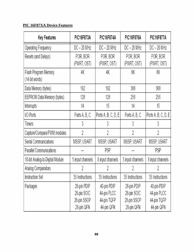
88

PIC 16F87XA Device Features

89

Special Function Register Summary

90

Appendix II

Operating Information of RS232 Interface

Recommended Operating Conditions

Electrical Characteristics over recommended ranges of supply voltage and operating free

air temperature

All Typical values are at Vcc = 5 V and Ta = 25°C

Test conditions Capacitor C1- C4 = 1µF at Vcc = 5V ± 0.5V

91

Step Down Transformer

Transformer Step down voltage according to the ratios of primary to secondary wire turns

Volt transformer ratio =

⁄

Current transformer ratio =

⁄

N = number of turns in winding

Post processor report of OrCAD

References:

1. Corporation, E. (2011) Environmental Impact of Emissions from Thermal Power

Generation in India. Volume, 04 DOI:

2. Shiv Pratap Raghuvanshi, A. C., Ashok Kumar Raghav (2005). Carbon dioxide

emissions from coal based power generation in India, Elsevier Ltd: 15.

3. Ramesh, J. (2010). India: Greenhouse Gas Emissions 2007, Indian Network for Climate

Change Assessment: 84.

4. Ananth P. Chikkatur, K. S. o. G. and C. Harvard University, MA (2008). A Resource

and Technology Assessment of Coal Utilization in India, Coal Initiative Reports: 52.

92

5. Enterprise, A.M.R.G.o.I. (2007). Neyveli M.o.C.a.f. fuels, fossil energy-government: 46

6. Brian Mc Pherson, Ning Liu, Yang Li, Liangxiong Li, Robert Lee (2006). Development

of a CO2 chemical sensor and strategy for CO2 monitoring in Carbon sequestration,

University of Utah, Salt lake city, USA :19

7. Bovensmann, H., Buchwitz, M., Burrows, J. P., Reuter, M., Krings, T., Gerilowski, K.,

Schneising, O., Heymann, J., Tretner, A., Erzinger, J. (2010): A remote sensing

technique for global monitoring of power plant CO2 emissions from space and related

applications. - Atmospheric Measurement Techniques, 3, 781-811

8. W.J Fisk, D.P Sullivan, D. Faulkner, E. Eliseeva (2010). CO2 Monitoring for demand

controlled ventilation in commercial buildings, Environmental Energy Technologies

Division, Lawrence Berkeley National Laboratory : 52

9. Jianwu Tang, Dennis D. Baldocchi, Ye Qi, Liukang Xu (2003). Assessing soil CO2

efflux using continuous measurement of CO2 profiles in soils with small solid-state

sensor, University of California, Elsevier Ltd: 14

10. IPCC, In: Houghton JT, Ding Y, Griggs DJ, Noguer M, Van der Linden PJ, Dai X, et al.,

editors. Climate Change 2001: A Scientific Basis: Intergovernmental Panel on Climate

Change. Cambridge, UK: Cambridge University Press; 2001.

11. M. Hung (2003): MQ2 Series Gas Sensor – Environmental Design Technology : 08

12. Microchip Technology 2003: PIC 16F87XA Data sheet- Pin Enhanced Flash

Microcontrollers: 234

13. Dogan Ibrahim, Elsevier 2010: SD card projects using PIC Microcontroller: 82.

14. Texas Instruments, Dallas, MAX 232, MAX 232I Dual EIA-232 Drivers/Receivers Data

sheet (2002): 09

15. Lammert Bias from the web source- http://www.lammertbies.nl/comm/info/RS-232_null_modem.html

16. TATA McGraw Hill (2005): Step Up/Step down transformers under web page

http://www.mhprofessional.com/downloads/products/0071494626/CroftCh5.pdf

17. Muhammad Ali Mazidi and Janice Gillispie Mazidi (2000). “ The 8051 Microcontroller and Embedded Systems” :94.

18. Kraig Mitzner (2007). Complete PCB Design Using OrCAD®Capture and Layout.

British Library Catalogue, Elsevier Ltd: 529

19. Visuvasam, D., Selvaraj, P. and Sekar, S., 2005. “Influence of Coal Properties on Particulate Emission Control in Thermal Power Plants in India.” Second International

Conference on Clean Coal Technologies for Our Future (CCT 2005), Sardinia, Italy.

20. MIN MEC Consultancy Pvt. Ltd, 2009. “E ecutive Summary of 2*500 MW Lignite

fired Neyveli New Thermal power Plant”, NLC: 21.

21. CEA, 2011. “CO2 baseline Database for the Indian Power Sector”- User Guide. Central

Electrical Authority, Government of India.

22. Marland and Rotty (1984), “IPCC Guidelines for national Greenhouse Gas

Inventories”: Volume 1.40, reference manual.

23. IPCC. Good Practice Guidance and Uncertainty Management in National Greenhouse

Gas Inventories. Intergovernmental Panel on Climate Change, National Greenhouse Gas

Inventories Program. May 2000.

24. NATCOM, 2004. India’s Initial National Communication to the UNFCC. Ministry of

Environment and Forests, Government of India.

93

25. IPCC AR4. 2007a. The Physical Science Basis. Working Group I Report of the

intergovernmental Panel on Climate Change. Editors: Solomon, S., D. Qin, M. Manning,

Z. Chen, M. Marquis, K.B. Averyt, M. Tignor and H.L. Miller. Cambridge University

Press, Cambridge, United Kingdom and New York, NY, USA.

26. Dunn S, Flavin C. Moving the climate change agenda forward: In State of the World

2002. Special World Summit Edition. NY: WW Norton and Company, 2002; p. 25–50.

27. Government of India- Department of Science and Technology, “Annual eport 2011-

2012”: 65-349.

28. Raghuvanshi SP, Chandra A, Raghav AK. Carbon dioxide emission inventory from

power sector. In: Proceedings Energy and Environment—International Conference on

Energy and Environment: Strategies for Sustainable Development (ICEE-SSD) 2004:

369–78.

29. NLC, 2009: “E ecutive Summary of 2*500 MW lignite fired Neyveli Lignite Thermal

Power plant” : MIN MEC Consultancy: 22

30. IPCC, 1992. Climate Change 1992: The Supplementary Report to the IPCC Scientific

Assessment. Report of the IPCC Scientific Assessment Working Group [Houghton, J.T.,

B.T. Callander and S.K. Varney (eds.)]. Cambridge University Press, Cambridge and

New York, 200 pp.

31. Kumar, Rakesh, Parag Jawale, and Shalini Tandon (2008). ‘Economic Impact of

Climate Change on Mumbai, India’, egional Health Forum, 12 (1), pp. 38–42.

32. evi, Aromar (2008). ‘Climate Change isk: An Adaptation and Mitigation Agenda for

Indian Cities’, Environment and Urbanization, 20(1), pp. 207–30, April.

33. IPCC (2007). ‘Summary for Policymakers’, in S. Solomon, D. Qin, M. Manning, Z.

Chen, M. Marquis, K.B. Averyt, M.Tignor, and H.L. Miller (eds), ‘Climate Change

2007: h e Physical Science Basis, Contribution of Working Group I to the Fourth

Assessment Report of the Intergovernmental Panel on Climate Change’, Cambridge

University Press, Cambridge, UK and New York.

34. Herzog H and E Drake, “Long-Term Advanced CO2 Capture Options,” Cheltenham,

U.K.: IEA/93/0E6; IEA Greenhouse Gas R&D Programme (1993).

35. Mimura T, H Simayoshi, T Suda, M Iijima and S Mituoka, “Development of Energy

Saving Technology for Flue Gas Carbon Dioxide Recovery by Chemical Absorption

Method and Steam System in Power Plant,” Energy Convers. Mgmt. Vol. 38, Suppl., pp.

S57-S62 (1997).

36. Herzog H, “The Economics of CO2 Capture,” P eimer, B Eliasson, A Wokaum, eds.,

Greenhouse Gas Control Technologies, Oxford: Elsevier Science Ltd., pp. 101-106

(1999).

37. Environmental Integrity Project, “ unning out of time – New U.S. EPA power plant

data shows greenhouse gases rising steadily”, March 2008.

38. Energy Information Administratio, URL: http://www.eia.doe.gov/fuelelectric.html.

39. P. Purohit, and A. Michaelowa, Potential of wind power projects under the Clean

Development Mechanism in India, Carbon Balance and Management, 2(8)

(doi:10.1186/1750-0680-2-8).

40. TNEB Reports, Daily online reports, at http://tnebldc.org/tnercreports.htm.

41. M. Suchitra, Windmills on tribal land, Down to Earth, Centre for Science and

Environment, New Delhi, 19(7), 2010.

94

42. C. H. Hansen, Bottom-up electricity reform using industrial captive generation: A case

study of Gujarat, India, Oxford Institute for Energy Studies, Mar. 2008, pp. 9

43. Bridge Rectifier waveform from the web source, URL: http://pecworld.zxq.net/Software/multisim/details/17_Single-Phase_full-Wave_Rectifiers.htm

44. California Polytechnic State University- Civil & Environmental Engineering

Department from the web source, URL: http://cr4.globalspec.com/thread/78868 45. Miura, J.; Holzinger, M.; Sitte, W. (1994). “Fast potentiometric CO2 sensors with open

reference electrodes.” Solid State Ionics, 74: 5-9

46. Lenntech, Water treatment Solutions for conversion from the web source, URL:

http://www.lenntech.com/calculators/ppm/converter-parts-per-million.htm

47. CO2 metering device downloaded from the web source, URL:

http://www.co2meter.com/page/downloads

48. Texas Instruments, Dallas, Sensors and field transmitters, “Design of gas sensor”. 1195-

2012: 09

49. Thomas B. eed, Agua Das (1998). “Bio mass down draft Gasifier Engine System Handbook”, 60-64: Volume 1.