Implementing Multidimensional Data Warehouses into NoSQL

Max Chevalier1, Mohammed El Malki

1,2, Arlind Kopliku

1, Olivier Teste

1 and Ronan Tournier

1

1 University of Toulouse, IRIT UMR 5505 (www.irit.fr), Toulouse, France 2Capgemini (www.capgemini.com), Toulouse, France

{Max.Chevalier, Mohammed.ElMalki, Arlind.Kopliku, Olivier.Teste, Ronan.Tournier}@irit.fr

Keywords: NoSQL, OLAP, Aggregate Lattice, Column-Oriented, Document-Oriented.

Abstract: Not only SQL (NoSQL) databases are becoming increasingly popular and have some interesting strengths

such as scalability and flexibility. In this paper, we investigate on the use of NoSQL systems for

implementing OLAP (On-Line Analytical Processing) systems. More precisely, we are interested in

instantiating OLAP systems (from the conceptual level to the logical level) and instantiating an aggregation

lattice (optimization). We define a set of rules to map star schemas into two NoSQL models: column-

oriented and document-oriented. The experimental part is carried out using the reference benchmark TPC.

Our experiments show that our rules can effectively instantiate such systems (star schema and lattice). We

also analyze differences between the two NoSQL systems considered. In our experiments, HBase (column-

oriented) happens to be faster than MongoDB (document-oriented) in terms of loading time.

1 INTRODUCTION

Nowadays, analysis data volumes are reaching

critical sizes (Jacobs, 2009) challenging traditional

data warehousing approaches. Current implemented

solutions are mainly based on relational databases

(using R-OLAP approaches) that are no longer

adapted to these data volumes (Stonebraker, 2012),

(Cuzzocrea et al., 2013), (Dehdouh et al., 2014).

With the rise of large Web platforms (e.g. Google,

Facebook, Twitter, Amazon, etc.) solutions for “Big

Data” management have been developed. These are

based on decentralized approaches managing large

data amounts and have contributed to developing

“Not only SQL” (NoSQL) data management

systems (Stonebraker, 2012). NoSQL solutions

allow us to consider new approaches for data

warehousing, especially from the multidimensional

data management point of view. This is the scope of

this paper.

In this paper, we investigate the use of NoSQL

models for decision support systems. Until now (and

to our knowledge), there are no mapping rules that

transform a multi-dimensional conceptual model

into NoSQL logical models. Existing research

instantiate OLAP systems in NoSQL through R-

OLAP systems; i.e., using an intermediate relational

logical model. In this paper, we define a set of rules

to translate automatically and directly a conceptual

multidimensional model into NoSQL logical

models. We consider two NoSQL logical models:

one column-oriented and one document-oriented.

For each model, we define mapping rules translating

from the conceptual level to the logical one. In

Figure 1, we position our approach based on

abstraction levels of information systems. The

conceptual level consists in describing the data in a

generic way regardless of information technologies

whereas the logical level consists in using a specific

technique for implementing the conceptual level.

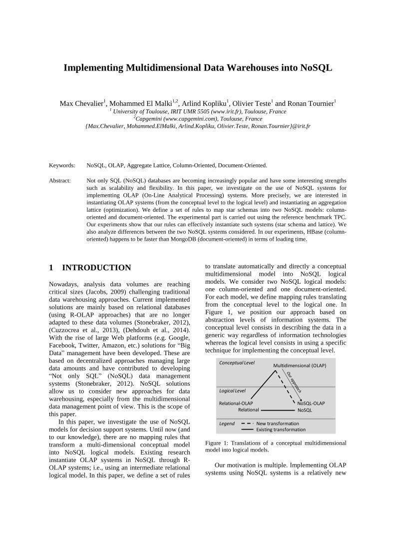
Figure 1: Translations of a conceptual multidimensional

model into logical models.

Our motivation is multiple. Implementing OLAP

systems using NoSQL systems is a relatively new

Multidimensional (OLAP)

Relational-OLAP

Conceptual Level

Logical Level

NoSQL-OLAPRelational NoSQL

New transformationExisting transformation

Legend

alternative. It is justified by advantages of these

systems such as flexibility and scalability. The

increasing research in this direction demands for

formalization, common models and empirical

evaluation of different NoSQL systems. In this

scope, this work contributes to investigate two

logical models and their respective mapping rules.

We also investigate data loading issues including

pre-computing data aggregates.

Traditionally, decision support systems use data

warehouses to centralize data in a uniform fashion

(Kimball et al., 2013). Within data warehouses,

interactive data analysis and exploration is

performed using On-Line Analytical Processing

(OLAP) (Colliat, 1996), (Chaudhuri et al., 1997).

Data is often described using a conceptual

multidimensional model, such as a star schema

(Chaudhuri et al., 1997). We illustrate this

multidimensional model with a case study about

RSS (Really Simple Syndication) feeds of news

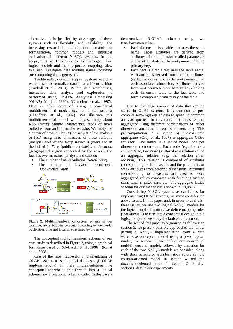
bulletins from an information website. We study the

Content of news bulletins (the subject of the analysis

or fact) using three dimensions of those bulletins

(analysis axes of the fact): Keyword (contained in

the bulletin), Time (publication date) and Location

(geographical region concerned by the news). The

fact has two measures (analysis indicators):

The number of news bulletins (NewsCount).

The number of keyword occurrences

(OccurrenceCount).

Figure 2: Multidimensional conceptual schema of our

example, news bulletin contents according to keywords,

publication time and location concerned by the news.

The conceptual multidimensional schema of our

case study is described in Figure 2, using a graphical

formalism based on (Golfarelli et al., 1998), (Ravat

et al., 2008).

One of the most successful implementation of

OLAP systems uses relational databases (R-OLAP

implementations). In these implementations, the

conceptual schema is transformed into a logical

schema (i.e. a relational schema, called in this case a

denormalized R-OLAP schema) using two

transformation rules:

Each dimension is a table that uses the same

name. Table attributes are derived from

attributes of the dimension (called parameters

and weak attributes). The root parameter is the

primary key.

Each fact is a table that uses the same name,

with attributes derived from 1) fact attributes

(called measures) and 2) the root parameter of

each associated dimension. Attributes derived

from root parameters are foreign keys linking

each dimension table to the fact table and

form a compound primary key of the table.

Due to the huge amount of data that can be

stored in OLAP systems, it is common to pre-

compute some aggregated data to speed up common

analysis queries. In this case, fact measures are

aggregated using different combinations of either

dimension attributes or root parameters only. This

pre-computation is a lattice of pre-computed

aggregates (Gray et al., 1997) or aggregate lattice

for short. The lattice is a set of nodes, one per

dimension combinations. Each node (e.g. the node

called “Time, Location”) is stored as a relation called

an aggregate relation (e.g. the relation time-

location). This relation is composed of attributes

corresponding to the measures and the parameters or

weak attributes from selected dimensions. Attributes

corresponding to measures are used to store

aggregated values computed with functions such as

SUM, COUNT, MAX, MIN, etc. The aggregate lattice

schema for our case study is shown in Figure 3.

Considering NoSQL systems as candidates for

implementing OLAP systems, we must consider the

above issues. In this paper and, in order to deal with

these issues, we use two logical NoSQL models for

the logical implementation; we define mapping rules

(that allows us to translate a conceptual design into a

logical one) and we study the lattice computation.

The rest of this paper is organized as follows: in

section 2, we present possible approaches that allow

getting a NoSQL implementation from a data

warehouse conceptual model using a pivot logical

model; in section 3 we define our conceptual

multidimensional model, followed by a section for

each of the two NoSQL models we consider along

with their associated transformation rules, i.e. the

column-oriented model in section 4 and the

document-oriented model in section 5. Finally,

section 6 details our experiments.

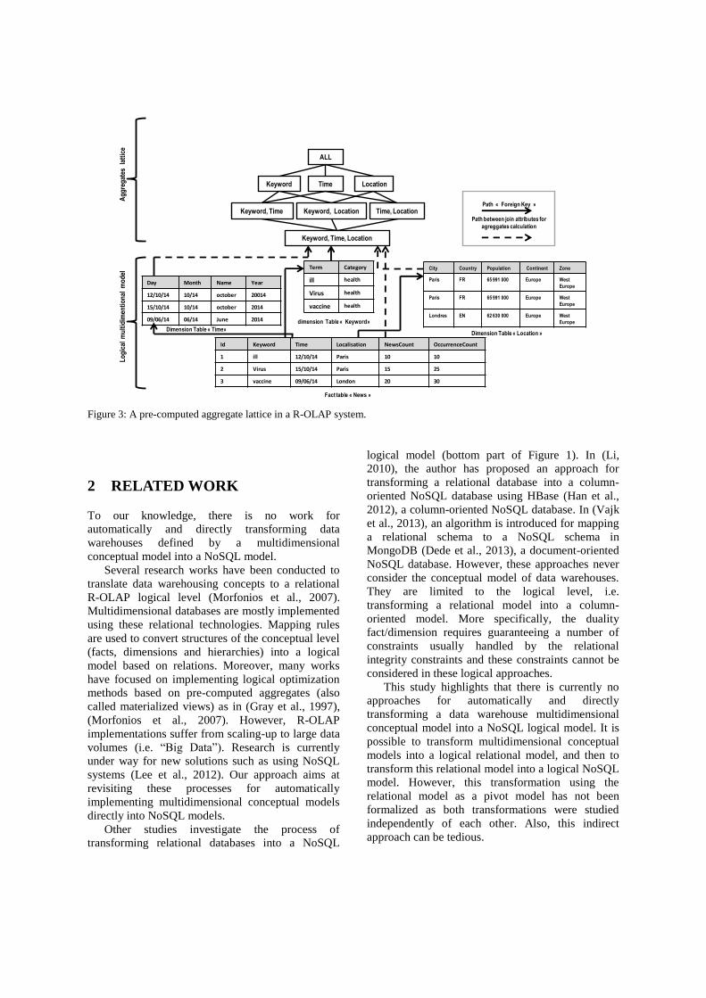
Figure 3: A pre-computed aggregate lattice in a R-OLAP system.

2 RELATED WORK

To our knowledge, there is no work for

automatically and directly transforming data

warehouses defined by a multidimensional

conceptual model into a NoSQL model.

Several research works have been conducted to

translate data warehousing concepts to a relational

R-OLAP logical level (Morfonios et al., 2007).

Multidimensional databases are mostly implemented

using these relational technologies. Mapping rules

are used to convert structures of the conceptual level

(facts, dimensions and hierarchies) into a logical

model based on relations. Moreover, many works

have focused on implementing logical optimization

methods based on pre-computed aggregates (also

called materialized views) as in (Gray et al., 1997),

(Morfonios et al., 2007). However, R-OLAP

implementations suffer from scaling-up to large data

volumes (i.e. “Big Data”). Research is currently

under way for new solutions such as using NoSQL

systems (Lee et al., 2012). Our approach aims at

revisiting these processes for automatically

implementing multidimensional conceptual models

directly into NoSQL models.

Other studies investigate the process of

transforming relational databases into a NoSQL

logical model (bottom part of Figure 1). In (Li,

2010), the author has proposed an approach for

transforming a relational database into a column-

oriented NoSQL database using HBase (Han et al.,

2012), a column-oriented NoSQL database. In (Vajk

et al., 2013), an algorithm is introduced for mapping

a relational schema to a NoSQL schema in

MongoDB (Dede et al., 2013), a document-oriented

NoSQL database. However, these approaches never

consider the conceptual model of data warehouses.

They are limited to the logical level, i.e.

transforming a relational model into a column-

oriented model. More specifically, the duality

fact/dimension requires guaranteeing a number of

constraints usually handled by the relational

integrity constraints and these constraints cannot be

considered in these logical approaches.

This study highlights that there is currently no

approaches for automatically and directly

transforming a data warehouse multidimensional

conceptual model into a NoSQL logical model. It is

possible to transform multidimensional conceptual

models into a logical relational model, and then to

transform this relational model into a logical NoSQL

model. However, this transformation using the

relational model as a pivot model has not been

formalized as both transformations were studied

independently of each other. Also, this indirect

approach can be tedious.

Id Keyword Time Localisation NewsCount OccurrenceCount

1 ill 12/10/14 Paris 10 10

2 Virus 15/10/14 Paris 15 25

3 vaccine 09/06/14 London 20 30

City Country Population Continent Zone

Paris FR 65 991 000 Europe West

Europe

Paris FR 65 991 000 Europe West

Europe

Londres EN 62 630 000 Europe West

Europe

Day Month Name Year

12/10/14 10/14 october 20014

15/10/14 10/14 october 2014

09/06/14 06/14 June 2014

Term Category

ill health

Virus health

vaccine health

Fact table « News »

Ag

gre

gat

es

latt

ice

Dimension Table « Time»Dimension Table « Location »

dimension Table « Keyword»

Path « Foreign Key »

Path between join attributes for

agreggates calculation

Keyword, Time, Location

Keyword, Time Keyword, Location Time, Location

Keyword Time Location

ALL

Lo

gic

al m

ult

idim

enti

on

alm

od

el

We can also cite several recent works that are

aimed at developing data warehouses in NoSQL

systems whether columns-oriented (Dehdouh et al.,

2014), or key-values oriented (Zhao et al., 2014).

However, the main goal of these papers is to propose

benchmarks. These studies have not put the focus on

the model transformation process. Likewise, they

only focus one NoSQL model, and limit themselves

to an abstraction at the HBase logical level. Both

models (Dehdouh et al., 2014), (Zhao et al., 2014),

require the relational model to be generated first

before the abstraction step. By contrast, we consider

the conceptual model as well as two orthogonal

logical models that allow distributing

multidimensional data either vertically using a

column-oriented model or horizontally using a

document-oriented model.

Finally we take into account hierarchies in our

transformation rules by providing transformation

rules to manage the aggregate lattice.

3 CONCEPTUAL MULTI-

DIMENSIONAL MODEL

To ensure robust translation rules we first define the

multidimensional model used at the conceptual

level.

A multidimensional schema, namely E, is

defined by (FE, D

E, Star

E) where:

FE = {F1,…, Fn} is a finite set of facts,

DE = {D1,…, Dm} is a finite set of dimensions,

StarE: F

E→

is a function that associates

each fact Fi of FE to a set of Di dimensions,

DiStarE(Fi), along which it can be analyzed;

note that is the power set of D

E.

A dimension, denoted DiDE (abusively noted

as D), is defined by (ND, A

D, H

D) where:

ND is the name of the dimension,

is a set of

dimension attributes,

is a set hierarchies.

A hierarchy of the dimension D, denoted

HiHD, is defined by (N

Hi, Param

Hi, Weak

Hi) where:

NHi

is the name of the hierarchy,

is

an ordered set of vi+2 attributes which are

called parameters of the relevant graduation

scale of the hierarchy, k[1..vi], A

D .

WeakHi

: ParamHi

is a function

associating with each parameter zero or more

weak attributes.

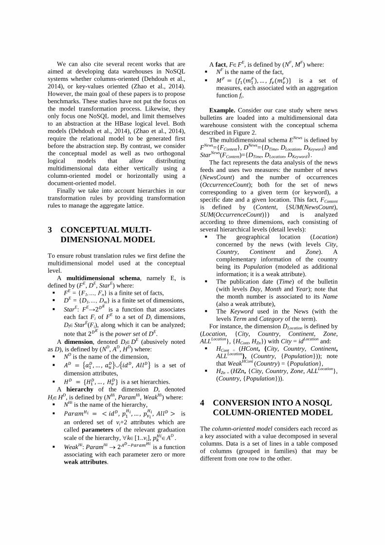
A fact, FFE, is defined by (N

F, M

F) where:

NF is the name of the fact,

is a set of

measures, each associated with an aggregation

function fi.

Example. Consider our case study where news

bulletins are loaded into a multidimensional data

warehouse consistent with the conceptual schema

described in Figure 2.

The multidimensional schema ENews

is defined by

FNews

={FContent}, DNews

={DTime, DLocation, DKeyword} and

StarNews

(FContent)={DTime, DLocation, DKeyword}.

The fact represents the data analysis of the news

feeds and uses two measures: the number of news

(NewsCount) and the number of occurrences

(OccurrenceCount); both for the set of news

corresponding to a given term (or keyword), a

specific date and a given location. This fact, FContent

is defined by (Content, {SUM(NewsCount),

SUM(OccurrenceCount)}) and is analyzed

according to three dimensions, each consisting of

several hierarchical levels (detail levels):

The geographical location (Location)

concerned by the news (with levels City,

Country, Continent and Zone). A

complementary information of the country

being its Population (modeled as additional

information; it is a weak attribute).

The publication date (Time) of the bulletin

(with levels Day, Month and Year); note that

the month number is associated to its Name

(also a weak attribute),

The Keyword used in the News (with the

levels Term and Category of the term).

For instance, the dimension DLocation is defined by

(Location, {City, Country, Continent, Zone,

ALLLocation

}, {HCont, HZn}) with City = idLocation

and:

HCont = (HCont, {City, Country, Continent,

ALLLocation

}, (Country, {Population})); note

that WeakHCont

(Country) = {Population},

HZn = (HZn, {City, Country, Zone, ALLLocation

},

(Country, {Population})).

4 CONVERSION INTO A NOSQL

COLUMN-ORIENTED MODEL

The column-oriented model considers each record as

a key associated with a value decomposed in several

columns. Data is a set of lines in a table composed

of columns (grouped in families) that may be

different from one row to the other.

4.1 NoSQL Column-Oriented Model

In relational databases, the data structure is

determined in advance with a limited number of

typed columns (a few thousand) each similar for all

records (also called “tuples”). Column-oriented

NoSQL models provide a flexible schema (untyped

columns) where the number of columns may vary

between each record (or “row”).

A column-oriented database (represented in

Figure 4) is a set of tables that are defined row by

row (but whose physical storage is organized by

groups of columns: column families; hence a

“vertical partitioning” of the data). In short, in these

systems, each table is a logical mapping of rows and

their column families. A column family can contain

a very large number of columns. For each row, a

column exists if it contains a value.

Figure 4: UML class diagram representing the concepts of

a column-oriented NoSQL database (tables, rows, column

families and columns).

A table T = {R1,…, Rn} is a set of rows Ri. A

row Ri = (Keyi, (CFi1,…, CFi

m)) is composed of a

row key Keyi and a set of column families CFij.

A column family CFij = {(Ci

j1, {vi

j1}),…, (Ci

jp,

{vijp

})} consists of a set of columns, each associated

with an atomic value. Every value can be

“historised” thanks to a timestamp. This principle

useful for version management (Wrembel, 2009)

will not be used in this paper due to limited space,

although it may be important.

The flexibility of a column-oriented NoSQL

database allows managing the absence of some

columns between the different table rows. However,

in the context of multidimensional data storage, data

is usually highly structured (Malinowski et al.,

2006). Thus, this implies that the structure of a

column family (i.e. the set of columns defined by the

column family) will be the same for all the table

rows. The initial structure is provided by the data

integration process called ETL, Extract, Transform,

and Load (Simitsis et al., 2005).

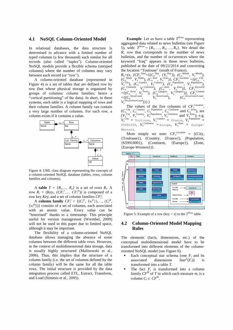
Example: Let us have a table TNews

representing

aggregated data related to news bulletins (see Figure

5), with: TNews

= {R1, …, Rx, …, Rn}. We detail the

Rx row that corresponds to the number of news

bulletins, and the number of occurrences where the

keyword “Iraq” appears in those news bulletins,

published at the date of 09/22/2014 and concerning

the location “Toulouse” (south of France).

Rx=(x, (CFxTime

={(CxDay

, {VxDay

}), (CxMonth

, VxMonth

),

(CxName

, VxName

), (CxYear

, VxYear

)}, CFxLocation

={(CxCity

,

VxCity

), (CxCountry

, VxCountry

), (CxPopulation

, VxPopulation

),

(CxContinent

, VxContinent

), (CxZone

, VxZone

)}, CFxKeyword

={(CxTerm

, VxTerm

), (CxCategory

, VxCategory

)}, CFxContent

={(CxNewsCount

, VxNewsCount

), (CxOccurrenceCount

,

VxOccurrenceCount

)}) )

The values of the five columns of CFxLocation

,

(CxCity

, CxCountry

, CxPopulation

, CxContinent

and CxZone

), are

(VxCity

, VxCountry

, VxPopulation

, VxContinent

and VxZone

); e.g.

VxCity

= Toulouse, VxCountry

= France, VxPopulation

=

65991000, VxContinent

= Europe, VxZone

= Europe-

Western.

More simply we note: CFxLocation

= {(City,

{Toulouse}), (Country, {France}), (Population,

{65991000}), (Continent, {Europe}), (Zone,

{Europe-Western})}.

Figure 5: Example of a row (key = x) in the TNews table.

4.2 Column-Oriented Model Mapping Rules

The elements (facts, dimensions, etc.) of the

conceptual multidimensional model have to be

transformed into different elements of the column-

oriented NoSQL model (see Figure 6).

Each conceptual star schema (one Fi and its

associated dimensions StarE(Fi)) is

transformed into a table T.

The fact Fi is transformed into a column

family CFM

of T in which each measure mi is a

column Ci CFM

.

Table

Name

1..*

1..*

1..*

1..1

1..1

Row

Key

Col. Family

Name

Columns

Name

Value

Val

Time Location KeyWord ContentId

Day

09/24/14

Month

09/14

Name

September

Year

2014

Term

Iraq

Category

Middle-East

NewsCount

2

OccurrenceCount

10

City

Toulouse

Country

France

Population

65991000

Continent

Europe

Zone

Europe-Western

x

... ... ... ...1

... ... ... ...n

...

...

Table TNews

Legend

Colomn

Identifier

Column

Family

Value

Continent

Europe

Location

Id

1

Lines of the Table

Each dimension Di StarE(F

i) is transformed

into a column family CFDi

where each

dimension attribute Ai AD (parameters and

weak attributes) is transformed into a column

Ci of the column family CFDi

(Ci CFDi

),

except the parameter AllDi

.

Remarks. Each fact instance and its associated

instances of dimensions are transformed into a row

Rx of T. The fact instance is thus composed of the

column family CFM

(the measures and their values)

and the column families of the dimensions CFDi

CFDE

(the attributes, i.e. parameters and weak

attributes, of each dimension and their values).

As in a denormalized R-OLAP star schema

(Kimball et al., 2013), the hierarchical organization

of the attributes of each dimension is not represented

in the NoSQL system. Nevertheless, hierarchies are

used to build the aggregate lattice. Note that the

hierarchies may also be used by the ETL processes

which build the instances respecting the constraints

induced by these conceptual structures (Malinowski

et al., 2006); however, we do not consider ETL

processes in this paper.

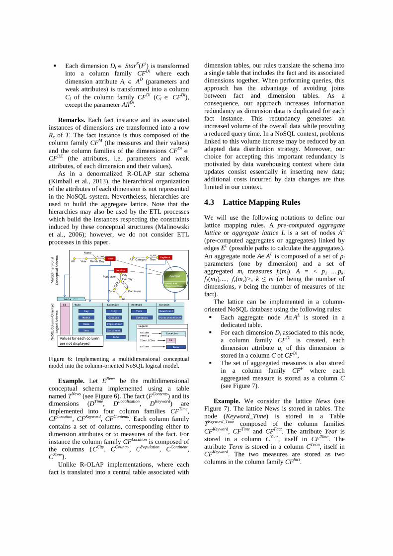
Figure 6: Implementing a multidimensional conceptual

model into the column-oriented NoSQL logical model.

Example. Let ENews

be the multidimensional

conceptual schema implemented using a table

named TNews

(see Figure 6). The fact (FContents

) and its

dimensions (DTime

, DLocalisation

, DKeyword

) are

implemented into four column families CFTime

,

CFLocation

, CFKeyword

, CFContents

. Each column family

contains a set of columns, corresponding either to

dimension attributes or to measures of the fact. For

instance the column family CFLocation

is composed of

the columns {CCity

, CCountry

, CPopulation

, CContinent

,

CZone

}.

Unlike R-OLAP implementations, where each

fact is translated into a central table associated with

dimension tables, our rules translate the schema into

a single table that includes the fact and its associated

dimensions together. When performing queries, this

approach has the advantage of avoiding joins

between fact and dimension tables. As a

consequence, our approach increases information

redundancy as dimension data is duplicated for each

fact instance. This redundancy generates an

increased volume of the overall data while providing

a reduced query time. In a NoSQL context, problems

linked to this volume increase may be reduced by an

adapted data distribution strategy. Moreover, our

choice for accepting this important redundancy is

motivated by data warehousing context where data

updates consist essentially in inserting new data;

additional costs incurred by data changes are thus

limited in our context.

4.3 Lattice Mapping Rules

We will use the following notations to define our

lattice mapping rules. A pre-computed aggregate

lattice or aggregate lattice L is a set of nodes AL

(pre-computed aggregates or aggregates) linked by

edges EL (possible paths to calculate the aggregates).

An aggregate node AAL is composed of a set of pi

parameters (one by dimension) and a set of

aggregated mi measures fi(mi). A = < p1 ....pk,

f1(m1),…, fv(mv)>, k ≤ m (m being the number of

dimensions, v being the number of measures of the

fact).

The lattice can be implemented in a column-

oriented NoSQL database using the following rules:

Each aggregate node AAL is stored in a

dedicated table.

For each dimension Di associated to this node,

a column family CFDi

is created, each

dimension attribute ai of this dimension is

stored in a column C of CFDi

,

The set of aggregated measures is also stored

in a column family CFF where each

aggregated measure is stored as a column C

(see Figure 7).

Example. We consider the lattice News (see

Figure 7). The lattice News is stored in tables. The

node (Keyword_Time) is stored in a Table

TKeyword_Time

composed of the column families

CFKeyword

, CFTime

and CFFact

. The attribute Year is

stored in a column CYear

, itself in CFTime

. The

attribute Term is stored in a column CTerm

, itself in

CFKeyword

. The two measures are stored as two

columns in the column family CFfact

.

Mu

ltid

imen

sio

nal

Co

nce

ptu

al S

chem

aN

oSQ

L C

olu

mn

-Ori

ente

dLo

gica

l Sch

ema

City

CountryPopulation

Zone Continent

All

Location

Time

DayMonthYearAll

Name

H_TIME KeyWordTermCategoryAll

H_KW

NewsCountOccurrenceCount

CONTENT

Day

Month

Name

Year

Term

Category

NewsCount

OccurrenceCount

City

Country

Population

Continent

Zone

Time Location KeyWord ContentId

Table TNews

Legend

Column

Identifier

Column

Family

Zone

Location

IdValues for each columnare not displayed

Many studies have been conducted about how to

select the pre-computed aggregates that should be

computed. In our proposition we favor computing all

aggregates (Kimball et al., 2013). This choice may

be sensitive due to the increase in the data volume.

However, in a NoSQL architecture we consider that

storage space should not be a major issue.

Figure 7: Implementing the pre-computed aggregation

lattice into a column-oriented NoSQL logical model.

5 CONVERSION INTO A NOSQL

DOCUMENT-ORIENTED

MODEL

The document-oriented model considers each record

as a document, which means a set of records

containing “attribute/value” pairs; these values are

either atomic or complex (embedded in sub-records).

Each sub-record can be assimilated as a document,

i.e. a subdocument.

5.1 NoSQL Document-Oriented Model

In the document-oriented model, each key is

associated with a value structured as a document.

These documents are grouped into collections. A

document is a hierarchy of elements which may be

either atomic values or documents. In the NoSQL

approach, the schema of documents is not

established in advance (hence the “schema less”

concept).

Formally, a NoSQL document-oriented database

can be defined as a collection C composed of a set of

documents Di, C = {D1,…, Dn}.

Each Di document is defined by a set of pairs

Di = {( ,

),…, ( ,

)}, j [1, m] where

Attij is an attribute (which is similar to a key) and Vi

j

is a value that can be of two forms:

The value is atomic.

The value is itself composed by a nested

document that is defined as a new set of pairs

(attribute, value).

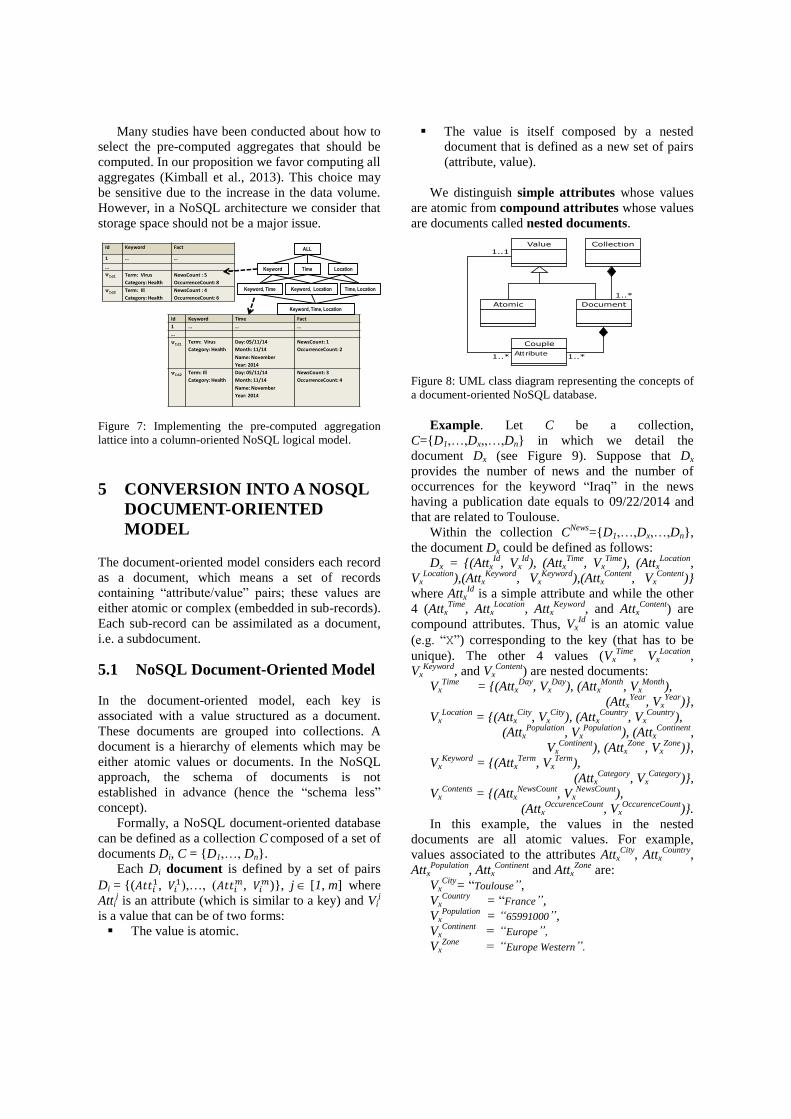
We distinguish simple attributes whose values

are atomic from compound attributes whose values

are documents called nested documents.

Figure 8: UML class diagram representing the concepts of

a document-oriented NoSQL database.

Example. Let C be a collection,

C={D1,…,Dx,,…,Dn} in which we detail the

document Dx (see Figure 9). Suppose that Dx

provides the number of news and the number of

occurrences for the keyword “Iraq” in the news

having a publication date equals to 09/22/2014 and

that are related to Toulouse.

Within the collection CNews

={D1,…,Dx,…,Dn},

the document Dx could be defined as follows:

Dx = {(AttxId

, VxId

), (AttxTime

, VxTime

), (AttxLocation

,

VxLocation

),(AttxKeyword

, VxKeyword

),(AttxContent

, VxContent

)}

where AttxId

is a simple attribute and while the other

4 (AttxTime

, AttxLocation

, AttxKeyword

, and AttxContent

) are

compound attributes. Thus, VxId

is an atomic value

(e.g. “X”) corresponding to the key (that has to be

unique). The other 4 values (VxTime

, VxLocation

,

VxKeyword

, and VxContent

) are nested documents:

VxTime

= {(AttxDay

, VxDay

), (AttxMonth

, VxMonth

),

(AttxYear

, VxYear

)},

VxLocation

= {(AttxCity

, VxCity

), (AttxCountry

, VxCountry

),

(AttxPopulation

, VxPopulation

), (AttxContinent

,

VxContinent

), (AttxZone

, VxZone

)},

VxKeyword

= {(AttxTerm

, VxTerm

),

(AttxCategory

, VxCategory

)},

VxContents

= {(AttxNewsCount

, VxNewsCount

),

(AttxOccurenceCount

, VxOccurenceCount

)}.

In this example, the values in the nested

documents are all atomic values. For example,

values associated to the attributes AttxCity

, AttxCountry

,

AttxPopulation

, AttxContinent

and AttxZone

are:

VxCity

= “Toulouse”,

VxCountry

= “France”,

VxPopulation

= “65991000”,

VxContinent

= “Europe”,

VxZone

= “Europe Western”.

Id Keyword Fact

1 … …

…

vId1 Term: Virus

Category: Health

NewsCount : 5

OccurrenceCount: 8

vId2 Term: Ill

Category: Health

NewsCount : 4

OccurrenceCount: 6

Id Keyword Time Fact

1 … … …

…

vId1 Term: Virus

Category: Health

Day: 05/11/14

Month: 11/14

Name: November

Year: 2014

NewsCount: 1

OccurrenceCount: 2

vId2 Term: Ill

Category: Health

Day: 05/11/14

Month: 11/14

Name: November

Year: 2014

NewsCount: 3

OccurrenceCount: 4

Keyword, Time, Location

Keyword, Time Keyword, Location Time, Location

Keyword Time Location

ALLCollection

DocumentAtomic

Couple

Attribute

Value

1..*

1..* 1..*

1..1

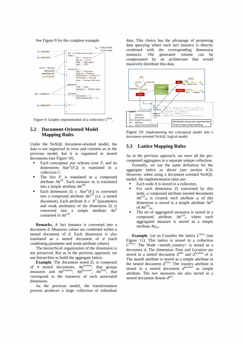
See Figure 9 for the complete example.

Figure 9: Graphic representation of a collection CNews.

5.2 Document-Oriented Model Mapping Rules

Under the NoSQL document-oriented model, the

data is not organized in rows and columns as in the

previous model, but it is organized in nested

documents (see Figure 10).

Each conceptual star schema (one Fi and its

dimensions StarE(Fi)) is translated in a

collection C.

The fact Fi is translated in a compound

attribute AttCF

. Each measure mi is translated

into a simple attribute AttSM

.

Each dimension Di StarE(Fi) is converted

into a compound attribute AttCD

(i.e. a nested

document). Each attribute Ai AD (parameters

and weak attributes) of the dimension Di is

converted into a simple attribute AttA

contained in AttCD

.

Remarks. A fact instance is converted into a

document d. Measures values are combined within a

nested document of d. Each dimension is also

translated as a nested document of d (each

combining parameter and weak attribute values).

The hierarchical organization of the dimension is

not preserved. But as in the previous approach, we

use hierarchies to build the aggregate lattice.

Example. The document noted Dx is composed

of 4 nested documents, AttContent

, that groups

measures and AttLocation

, AttKeyword

, AttTime

, that

correspond to the instances of each associated

dimension.

As the previous model, the transformation

process produces a large collection of redundant

data. This choice has the advantage of promoting

data querying where each fact instance is directly

combined with the corresponding dimension

instances. The generated volume can be

compensated by an architecture that would

massively distribute this data.

Figure 10: Implementing the conceptual model into a

document-oriented NoSQL logical model.

5.3 Lattice Mapping Rules

As in the previous approach, we store all the pre-

computed aggregates in a separate unique collection.

Formally, we use the same definition for the

aggregate lattice as above (see section 4.3).

However, when using a document oriented NoSQL

model, the implementation rules are:

Each node A is stored in a collection.

For each dimension Di concerned by this

node, a compound attribute (nested document)

AttCD

Di is created; each attribute ai of this

dimension is stored in a simple attribute Attai

of AttCD

Di.

The set of aggregated measures is stored in a

compound attribute AttCD

F where each

aggregated measure is stored as a simple

attribute Attmi.

Example. Let us Consider the lattice LNews

(see

Figure 11). This lattice is stored in a collection

CNews

. The Node <month_country> is stored as a

document d. The dimension Time and Location are

stored in a nested document ddate

and dlocation

of d.

The month attribute is stored as a simple attribute in

the nested document dTime

. The country attribute is

stored in a nested document dlocation

as simple

attribute. The two measures are also stored in a

nested document denote dfact

.

{} Collection() DocumentAtt: {} Nested DocumentAtt: AttributevAtt Value of the Att Attribute

Legend

{

(Id : vIdTime : {Day: vDa, Month: vMo, Name: vNa, Year: vYe}

Location: {City: vCi, Country: vCtr, Population: vPo,

Continent: vCnt, Zone: vZn}

KeyWord : {Term: vTe, Category: vCa}

Content : {NewsCount: vNCt, OccurrenceCount: vOCt} )

( Id … )

…

}

Time

Day Month Year All

Name

H_TIME

KeyWord

Term Category All

H_KW

NewsCountOccurenceCount

CONTENTPopulation

City

Location

Country

ContinentZone

All

Attributes values are representedonly to ease understanding

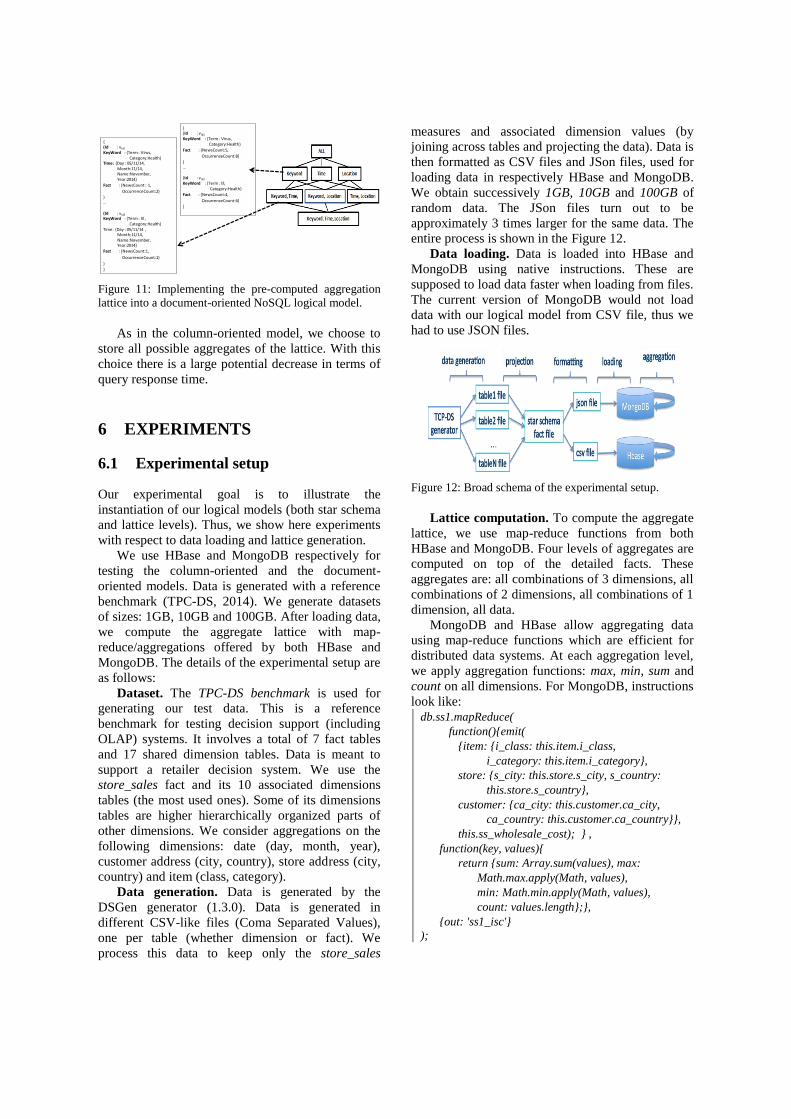
Figure 11: Implementing the pre-computed aggregation

lattice into a document-oriented NoSQL logical model.

As in the column-oriented model, we choose to

store all possible aggregates of the lattice. With this

choice there is a large potential decrease in terms of

query response time.

6 EXPERIMENTS

6.1 Experimental setup

Our experimental goal is to illustrate the

instantiation of our logical models (both star schema

and lattice levels). Thus, we show here experiments

with respect to data loading and lattice generation.

We use HBase and MongoDB respectively for

testing the column-oriented and the document-

oriented models. Data is generated with a reference

benchmark (TPC-DS, 2014). We generate datasets

of sizes: 1GB, 10GB and 100GB. After loading data,

we compute the aggregate lattice with map-

reduce/aggregations offered by both HBase and

MongoDB. The details of the experimental setup are

as follows:

Dataset. The TPC-DS benchmark is used for

generating our test data. This is a reference

benchmark for testing decision support (including

OLAP) systems. It involves a total of 7 fact tables

and 17 shared dimension tables. Data is meant to

support a retailer decision system. We use the

store_sales fact and its 10 associated dimensions

tables (the most used ones). Some of its dimensions

tables are higher hierarchically organized parts of

other dimensions. We consider aggregations on the

following dimensions: date (day, month, year),

customer address (city, country), store address (city,

country) and item (class, category).

Data generation. Data is generated by the

DSGen generator (1.3.0). Data is generated in

different CSV-like files (Coma Separated Values),

one per table (whether dimension or fact). We

process this data to keep only the store_sales

measures and associated dimension values (by

joining across tables and projecting the data). Data is

then formatted as CSV files and JSon files, used for

loading data in respectively HBase and MongoDB.

We obtain successively 1GB, 10GB and 100GB of

random data. The JSon files turn out to be

approximately 3 times larger for the same data. The

entire process is shown in the Figure 12.

Data loading. Data is loaded into HBase and

MongoDB using native instructions. These are

supposed to load data faster when loading from files.

The current version of MongoDB would not load

data with our logical model from CSV file, thus we

had to use JSON files.

Figure 12: Broad schema of the experimental setup.

Lattice computation. To compute the aggregate

lattice, we use map-reduce functions from both

HBase and MongoDB. Four levels of aggregates are

computed on top of the detailed facts. These

aggregates are: all combinations of 3 dimensions, all

combinations of 2 dimensions, all combinations of 1

dimension, all data.

MongoDB and HBase allow aggregating data

using map-reduce functions which are efficient for

distributed data systems. At each aggregation level,

we apply aggregation functions: max, min, sum and

count on all dimensions. For MongoDB, instructions

look like: db.ss1.mapReduce(

function(){emit(

{item: {i_class: this.item.i_class,

i_category: this.item.i_category},

store: {s_city: this.store.s_city, s_country:

this.store.s_country},

customer: {ca_city: this.customer.ca_city,

ca_country: this.customer.ca_country}},

this.ss_wholesale_cost); } ,

function(key, values){

return {sum: Array.sum(values), max:

Math.max.apply(Math, values),

min: Math.min.apply(Math, values),

count: values.length};},

{out: 'ss1_isc'}

);

{(Id : vId1

KeyWord : {Term : Virus, Category:Health}

Fact : {NewsCount:5,

OccurrenceCount:8}

)…

(Id : vId2

KeyWord : {Term : Ill,Category:Health}

Fact : {NewsCount:4,

OccurrenceCount:6)

}

{(Id : vId1

KeyWord : {Term : Virus,Category:Health}

Time: {Day : 05/11/14,Month:11/14,Name:November,Year:2014}

Fact : {NewsCount : 1,

OccurrenceCount:2}

)…

(Id : vId2

KeyWord : {Term : Ill ,Category:Health}

Time: {Day : 05/11/14 ,Month:11/14,Name:November,Year:2014}

Fact : {NewsCount:1,

OccurrenceCount:1}

)

}

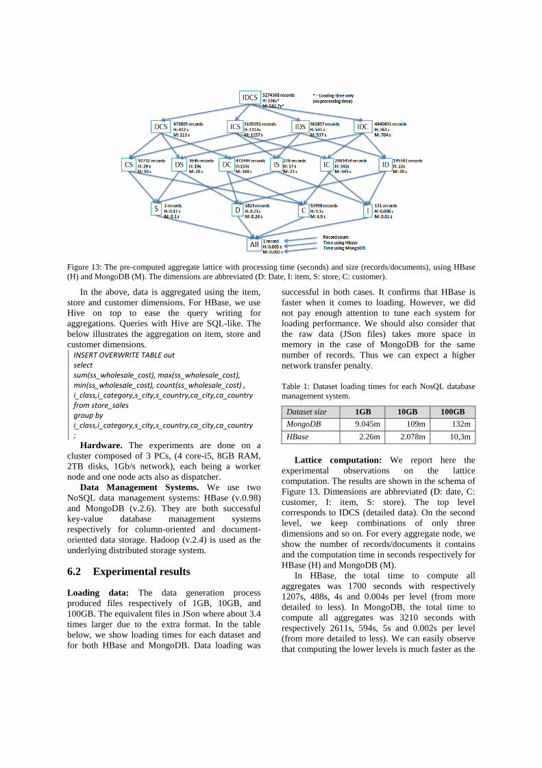
Figure 13: The pre-computed aggregate lattice with processing time (seconds) and size (records/documents), using HBase

(H) and MongoDB (M). The dimensions are abbreviated (D: Date, I: item, S: store, C: customer).

In the above, data is aggregated using the item,

store and customer dimensions. For HBase, we use

Hive on top to ease the query writing for

aggregations. Queries with Hive are SQL-like. The

below illustrates the aggregation on item, store and

customer dimensions. INSERT OVERWRITE TABLE out select sum(ss_wholesale_cost), max(ss_wholesale_cost), min(ss_wholesale_cost), count(ss_wholesale_cost) , i_class,i_category,s_city,s_country,ca_city,ca_country from store_sales group by i_class,i_category,s_city,s_country,ca_city,ca_country ;

Hardware. The experiments are done on a

cluster composed of 3 PCs, (4 core-i5, 8GB RAM,

2TB disks, 1Gb/s network), each being a worker

node and one node acts also as dispatcher.

Data Management Systems. We use two

NoSQL data management systems: HBase (v.0.98)

and MongoDB (v.2.6). They are both successful

key-value database management systems

respectively for column-oriented and document-

oriented data storage. Hadoop (v.2.4) is used as the

underlying distributed storage system.

6.2 Experimental results

Loading data: The data generation process

produced files respectively of 1GB, 10GB, and

100GB. The equivalent files in JSon where about 3.4

times larger due to the extra format. In the table

below, we show loading times for each dataset and

for both HBase and MongoDB. Data loading was

successful in both cases. It confirms that HBase is

faster when it comes to loading. However, we did

not pay enough attention to tune each system for

loading performance. We should also consider that

the raw data (JSon files) takes more space in

memory in the case of MongoDB for the same

number of records. Thus we can expect a higher

network transfer penalty.

Table 1: Dataset loading times for each NosQL database

management system.

Dataset size 1GB 10GB 100GB

MongoDB 9.045m 109m 132m

HBase 2.26m 2.078m 10,3m

Lattice computation: We report here the

experimental observations on the lattice

computation. The results are shown in the schema of

Figure 13. Dimensions are abbreviated (D: date, C:

customer, I: item, S: store). The top level

corresponds to IDCS (detailed data). On the second

level, we keep combinations of only three

dimensions and so on. For every aggregate node, we

show the number of records/documents it contains

and the computation time in seconds respectively for

HBase (H) and MongoDB (M).

In HBase, the total time to compute all

aggregates was 1700 seconds with respectively

1207s, 488s, 4s and 0.004s per level (from more

detailed to less). In MongoDB, the total time to

compute all aggregates was 3210 seconds with

respectively 2611s, 594s, 5s and 0.002s per level

(from more detailed to less). We can easily observe

that computing the lower levels is much faster as the

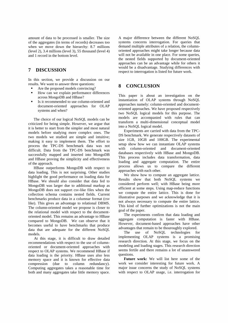
amount of data to be processed is smaller. The size

of the aggregates (in terms of records) decreases too

when we move down the hierarchy: 8.7 millions

(level 2), 3.4 millions (level 3), 55 thousand (level 4)

and 1 record in the bottom level.

7 DISCUSSION

In this section, we provide a discussion on our

results. We want to answer three questions:

Are the proposed models convincing?

How can we explain performance differences

across MongoDB and HBase?

Is it recommended to use column-oriented and

document-oriented approaches for OLAP

systems and when?

The choice of our logical NoSQL models can be

criticized for being simple. However, we argue that

it is better to start from the simpler and most natural

models before studying more complex ones. The

two models we studied are simple and intuitive;

making it easy to implement them. The effort to

process the TPC-DS benchmark data was not

difficult. Data from the TPC-DS benchmark was

successfully mapped and inserted into MongoDB

and HBase proving the simplicity and effectiveness

of the approach.

HBase outperforms MongoDB with respect to

data loading. This is not surprising. Other studies

highlight the good performance on loading data for

HBase. We should also consider that data fed to

MongoDB was larger due to additional markup as

MongoDB does not support csv-like files when the

collection schema contains nested fields. Current

benchmarks produce data in a columnar format (csv

like). This gives an advantage to relational DBMS.

The column-oriented model we propose is closer to

the relational model with respect to the document-

oriented model. This remains an advantage to HBase

compared to MongoDB. We can observe that it

becomes useful to have benchmarks that produce

data that are adequate for the different NoSQL

models. At this stage, it is difficult to draw detailed

recommendations with respect to the use of column-oriented or document-oriented approaches with respect to OLAP systems. We recommend HBase if data loading is the priority. HBase uses also less memory space and it is known for effective data compression (due to column redundancy). Computing aggregates takes a reasonable time for both and many aggregates take little memory space.

A major difference between the different NoSQL systems concerns interrogation. For queries that demand multiple attributes of a relation, the column-oriented approaches might take longer because data will not be available in one place. For some queries, the nested fields supported by document-oriented approaches can be an advantage while for others it would be a disadvantage. Studying differences with respect to interrogation is listed for future work.

8 CONCLUSION

This paper is about an investigation on the

instantiation of OLAP systems through NoSQL

approaches namely: column-oriented and document-

oriented approaches. We have proposed respectively

two NoSQL logical models for this purpose. The

models are accompanied with rules that can

transform a multi-dimensional conceptual model

into a NoSQL logical model.

Experiments are carried with data from the TPC-

DS benchmark. We generate respectively datasets of

size 1GB, 10GB and 100GB. The experimental

setup show how we can instantiate OLAP systems

with column-oriented and document-oriented

databases respectively with HBase and MongoDB.

This process includes data transformation, data

loading and aggregate computation. The entire

process allows us to compare the different

approaches with each other.

We show how to compute an aggregate lattice.

Results show that both NoSQL systems we

considered perform well; with HBase being more

efficient at some steps. Using map-reduce functions

we compute the entire lattice. This is done for

illustrative purposes and we acknowledge that it is

not always necessary to compute the entire lattice.

This kind of further optimizations is not the main

goal of the paper.

The experiments confirm that data loading and

aggregate computation is faster with HBase.

However, document-based approaches have other

advantages that remain to be thouroughly explored.

The use of NoSQL technologies for

implementing OLAP systems is a promising

research direction. At this stage, we focus on the

modeling and loading stages. This research direction

seems fertile and there remains a lot of unanswered

questions.

Future work: We will list here some of the

work we consider interesting for future work. A

major issue concerns the study of NoSQL systems

with respect to OLAP usage, i.e. interrogation for

analysis purposes. We need to study the different

types of queries and identify queries that benefit

mostly for NoSQL models.

Finally, all approaches (relational models,

NoSQL models) should be compared with each

other in the context of OLAP systems. We can also

consider different NoSQL logical ilmplementations.

We have proposed simple models and we want to

compare them with more complex and optimized

ones.

In addition, we believe that it is timely to build

benchmarks for OLAP systems that generalize to

NoSQL systems. These benchmarks should account

for data loading and database usage. Most existing

benchmarks favor relational models.

ACKNOWLEDGEMENTS

These studies are supported by the ANRT funding under CIFRE-Capgemini partnership.

REFERENCES

Chaudhuri, S., Dayal, U., 1997. An overview of data

warehousing and olap technology. SIGMOD Record,

26, ACM, pp. 65–74.

Colliat, G., 1996. Olap, relational, and multidimensional

database systems. SIGMOD Record, 25(3), ACM, pp.

64–69.

Cuzzocrea, A., Bellatreche, L., Song, I.-Y., 2013. Data

warehousing and olap over big data: Current

challenges and future research directions. 16th Int.

Workshop on Data Warehousing and OLAP

(DOLAP), ACM, pp. 67–70.

Dede, E., Govindaraju, M., Gunter, D., Canon, R. S.,

Ramakrishnan, L., 2013. Performance evaluation of a

mongodb and hadoop platform for scientific data

analysis. 4th Workshop on Scientific Cloud

Computing, ACM, pp. 13–20.

Dehdouh, K., Boussaid, O., Bentayeb, F., 2014. Columnar

nosql star schema benchmark. Model and Data

Engineering, LNCS 8748, Springer, pp. 281–288.

Golfarelli, M., Maio, D., and Rizzi, S., 1998. The

dimensional fact model: A conceptual model for data

warehouses. Int. Journal of Cooperative Information

Systems, 7, pp. 215–247.

Gray, J., Bosworth, A., Layman, A., Pirahesh, H., 1996.

Data Cube: A Relational Aggregation Operator

Generalizing Group-By, Cross-Tab, and Sub-Total.

Int. Conf. on Data Engineering (ICDE), IEEE

Computer Society, pp. 152-159.

Han, D., Stroulia, E., 2012. A three-dimensional data

model in hbase for large time-series dataset analysis.

6th Int. Workshop on the Maintenance and Evolution

of Service-Oriented and Cloud-Based Systems

(MESOCA), IEEE, pages 47–56.

Jacobs, A., 2009. The pathologies of big data.

Communications of the ACM, 52(8), pp. 36–44.

Kimball, R. Ross, M., 2013. The Data Warehouse Toolkit:

The Definitive Guide to Dimensional Modeling. John

Wiley & Sons, Inc., 3rd edition.

Lee, S., Kim, J., Moon, Y.-S., Lee, W., 2012. Efficient

distributed parallel top-down computation of R-OLAP

data cube using mapreduce. Int conf. on Data

Warehousing and Knowledge Discovery (DaWaK),

LNCS 7448, Springer, pp. 168–179.

Li, C., 2010. Transforming relational database into hbase:

A case study. Int. Conf. on Software Engineering and

Service Sciences (ICSESS), IEEE, pp. 683–687.

Malinowski, E., Zimányi, E., 2006. Hierarchies in a

multidimensional model: From conceptual modeling

to logical representation. Data and Knowledge

Engineering, 59(2), Elsevier, pp. 348–377.

Morfonios, K., Konakas, S., Ioannidis, Y., Kotsis, N.,

2007. R-OLAP implementations of the data cube.

ACM Computing Survey, 39(4), p. 12.

Simitsis, A., Vassiliadis, P., Sellis, T., 2005. Optimizing

etl processes in data warehouses. Int. Conf. on Data

Engineering (ICDE), IEEE, pp. 564–575.

Ravat, F., Teste, O., Tournier, R., Zurfluh, G., 2008.

Algebraic and Graphic Languages for OLAP

Manipulations. Int. journal of Data Warehousing and

Mining (ijDWM), 4(1), IGI Publishing, pp. 17-46.

Stonebraker, M., 2012. New opportunities for new sql.

Communications of the ACM, 55(11), pp. 10–11.

Vajk, T., Feher, P., Fekete, K., Charaf, H., 2013.

Denormalizing data into schema-free databases. 4th

Int. Conf. on Cognitive Infocommunications

(CogInfoCom), IEEE, pp. 747–752.

Vassiliadis, P., Vagena, Z., Skiadopoulos, S.,

Karayannidis, N., 2000. ARKTOS: A Tool For Data

Cleaning and Transformation in Data Warehouse

Environments. IEEE Data Engineering Bulletin, 23(4),

pp. 42-47.

TPC-DS, 2014. Transaction Processing Performance

Council, Decision Support benchmark, version 1.3.0,

http://www.tpc.org/tpcds/.

Wrembel, R., 2009. A survey of managing the evolution

of data warehouses. Int. Journal of Data Warehousing

and Mining (ijDWM), 5(2), IGI Publishing, pp. 24–56.

Zhao, H., Ye, X., 2014. A practice of tpc-ds

multidimensional implementation on nosql database

systems. 5th TPC Tech. Conf. Performance

Characterization and Benchmarking, LNCS 8391,

Springer, pp. 93–108.