IMPLEMENTING THE FAST MULTIPOLE BOUNDARY ELEMENT

METHOD WITH HIGH-ORDER ELEMENTS

A. Gee∗, B. Erdelyi†

Physics Dept., Northern Illinois University, DeKalb, IL 60115, USA

Abstract

The next generation of beam applications will require

high-intensity beams with unprecedented control. For the

new system designs, simulations that model collective effects

must achieve greater accuracies and scales than conventional

methods allow. The fast multipole method is a strong candi-

date for modeling collective effects due to its linear scaling.

It is well known the boundary effects become important for

such intense beams. We implemented a constant element

fast boundary element method (FMBEM) [2] as our first

step in studying the boundary effects. To reduce the number

of elements and discretization error, our next step is to allow

for curvilinear elements. In this paper, we will present our

study on a quadratic and a cubic parametric method to model

the surface.

INTRODUCTION

Beam applications have grown in the last few decades

as has the need for precise control, particularly for high-

intensity beams. However, collective and boundary effects

become significant at such intensities. Conventional lattices

are insufficient to prevent undesirable behavior. To facilitate

future lattice designs, simulation models such as N-body

solvers are being developed for large scale problems. In

particular, the fast multipole method (FMM) is a strong

candidate as a N-body solver due to its O(N ) scaling.

It is well known effects due to the beam pipe become

important for high-intensity beams. To include boundary

conditions for complicated structures, the boundary element

method (BEM) has shown excellent results in various fields.

However, the dense system matrix of size M can lead to

O(M3) scaling in the worst scenario. The FMM has been

used to accelerate the BEM, improving the scaling signifi-

cantly [1]. In previous work, we combined our FMM mod-

ule with a constant element BEM [2]. However, our results

suggested the accuracy is strongly limited by the discretiza-

tion error from flat panel elements. Parametric curvilinear

elements are expected to improve the accuracy and perfor-

mance of the FMBEM. We evaluated an analytical quadratic

patch [3] and a constructive cubic patch [4] which use unit

normals.

THEORY

Our constant element BEM in [2] was implemented using

the single layer potential formulation, which leads to an

ill-conditioned system [1]. We chose to continue using the

∗ agee1@niu.edu† berdelyi@niu.edu

double layer potential and the single layer field for Dirichlet

and Neumann type BC, respectively. Equations 1 and 2 give

the discretized integral equations with ∂G∂ny≡ n(y) · ∇yG.

φ(xi) =

M∑j=1

∫Γj

∂G

∂ny(xi, yj )η(yj )dΓ(y) (1)

∂φ

∂nx

(xi) =

M∑j=1

∫Γj

∂G

∂nx

(xi, yj )σ(yj )dΓ(y) (2)

From Eqs. 1 and 2 and the parametric area element,���∂x∂u× ∂x

∂v

���, it is imperative our parametrization gives accu-

rate normals on the element and interpolates the normals

at the vertices for continuity. We decided on two methods

given in [3] and [4].

Figure 1: Triangle in (u, v) with vertices x1 = x(0, 0), x2 =

x(1, 0), x3 = x(0, 1) and corresponding normals.

The quadratic patch in [3] fits an order 2 polynomial of

form x(u, v) = a00 + a10u + a01v + a20u2+ a11uv + a02v

2

given vertices x1, x2, x3 and normals n1, n2, n3. For a triangle

as in Fig. 1, the coefficients are given in Eq. 3. c(di j, ni, nj )

in Eq. 3 is termed the curvature parameter in [3] and can be

calculated by Eq. 4. [3] gives details on the derivation.

di j ≡ xj − xi

ci j ≡ c(di j, ni, nj )

a00 = x1

a10 = d12 − c12

a01 = d13 − c13

a20 = c12

a11 = c12 + c13 − c23

a02 = c23

(3)

ν =

ni + nj

2

∆ν =ni − nj

2

d = di j · ν

∆d = di j · ∆ν

c = 1 − 2∆c

∆c = ni · ∆ν

c(di j, ni, nj ) =

∆d

1 − ∆cν +

d

∆c∆ν c , ±1

0 c = ±1

(4)

TUPOB15 Proceedings of NAPAC2016, Chicago, IL, USA ISBN 978-3-95450-180-9

518Copy

right

©20

16CC

-BY-

3.0

and

byth

ere

spec

tive

auth

ors

5: Beam Dynamics and EM Fields

The cubic patch in [4] constructs a surface using order 3

polynomials by separately fitting over two edges sharing a

vertex and spanning a third curve across the patch. In [4], this

was purely constructive to calculate 10 points on the patch

and fit using Lagrange interpolation. However, we wished

to examine the constructed polynomials as an analytical

surface. The coefficients for the univariate cubic polynomial,

p(u) = a0 + a1u + a2u2+ a3u3, are given in Equation 5.

α =(x2 − x1) ·

[(n2 · n2)n1 +

12

(n1 · n2)n2

]

23

(n1 · n1)(n2 · n2) − 16

(n1 · n2)

β =−(x2 − x1) · n2 −

13

(n1 · n2)α

23

(n2 · n2)

a0 = x1

a1 = x2 − a0 − a2 − a3

a2 = αn1

a3 =1

3(βn2 − a2)

(5)

k(u) =1

���dp

du

���2

d2p

du2−

dp

du·d2p

du2

���dp

du

���2

dp

du

(6)

As in [4], we construct p12(u) and p13(u) and their nor-

mals k12(u) and k13(u) using Eq. 6, where i j refers to the

edge between vertices i and j. We then construct the span-

ning curve, x(u, v) = a0(u) + a1(u)v + a2(u)v2+ a3(u)v3,

where x1 → p12, x2 → p13, n1 → k12, n2 → k13, which

ultimately gives a bivariate cubic with (u, v) ∈ [0, 1]× [0, 1]

over the entire patch. This is mapped to the triangle in Fig.

1 as described by [4]. Normalization is only needed at the

end.

In [4], they impose the approximation, d2xdu2 ‖ n at the

endpoints. The effect of this approximation is unclear. The

constructed cubic polynomial x(u,v) [4] is cumbersome in

practice. We also evaluate the 3rd order Taylor expansion of

x(u, v) and corresponding normal for actual use.

ANALYSIS

The previous methods were implemented and tested using

a spherical triangle and a flat panel discretized sphere. The

centroids, unit normals and areas are easily computed and

provide a simple test in addition to testing the interpolation

conditions. The area element is tested by! ���

∂x∂u× ∂x

∂v

��� dudv.

The spherical triangle is formed by picking 3 points in the

first octant of a sphere centered at (0, 0, 0) with radius R and

forming the corresponding spherical arcs. This prevents an

angle > π

2between the normals. The spherical triangle area

is given by R2(A+ B +C − π) where A, B,C are the interior

angles and can be found in numerous ways. The parameters

for the spherical triangle are given in Table 1 and chosen for

a relatively large area to amplify the errors.

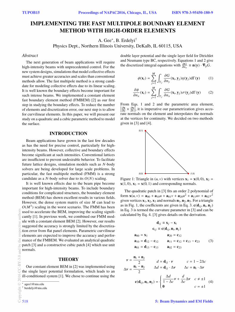
We represent the spherical triangle (green) in Fig. 2. The

quadratic patch showed good results for this case. Figure 2a

shows the patch (blue) has a slight deviation in the center

but represents the shape well. In Fig. 2b, the constructed

polynomial (blue) shows significant deviation around the

center but interpolates the vertices correctly. However, its

Table 1: Spherical Triangle Parameters

Vertices

(8.93, 4.49, 0.27)

(3.08, 6.60, 6.85)

(8.63, 0.54, 5.02)

Center (7.75, 4.37, 4.56)

Radius 10

Area 28.970

3rd order Taylor expansion (red) deviates significantly and

does not interpolate x3 at all.

(a) Quadratic patch (blue) (b) Cubic patch (blue) and

truncated cubic (red)

Figure 2: Comparison of parametric patches on the spherical

triangle (green) given by Table 1. In Figure 2a, the quadratic

patch (blue) deviates slightly in the center. In Figure 2b, the

patch using a cubic polynomial (blue) vs its 3rd order Taylor

expansion (red) deviate significantly in this case.

We evaluated the centroid and unit normal at (1/3, 1/3) for

the quadratic patch and equivalently (2/3, 1/2) for the cubic

patch mapped from Fig. 1. The percent errors are given in

Table 2. We show the L2-norm in the case of the centroid and

unit normal. The results suggest the truncation of the Taylor

expansion affected the area element significantly. Since the

parametric surface does not match, the error in the unit

normal for the truncated cubic is inconclusive.

Table 2: Percent Errors On Spherical Triangle

Centroid Normal Area

Quadratic 0.79 0.44 -0.33

Cubic 1.63 6.49 1.53

Truncated cubic 4.19 30.5 13.6

The previous results reflect the case of a large element. To

check with practical elements, we chose a sphere discretized

by flat panels or constant elements, where we know the

vertices and normals lie on the surface. In this case, only the

3rd order Taylor expansion could be evaluated for the cubic

patch. Following the same analysis, we checked the area,

centroid and unit normals for each element after verifying

similar behavior at vertices as before.

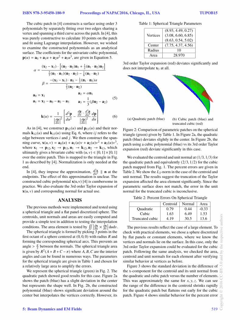
Figure 3 shows the standard deviation in the difference of

the x-component for the centroid and its unit normal from

the quadratic and cubic patch versus the number of elements.

This was approximately the same for x, y, z. We can see

the range of the difference in the centroid shrinks rapidly

for the quadratic patch but flattens out early for the cubic

patch. Figure 4 shows similar behavior for the percent error

ISBN 978-3-95450-180-9 Proceedings of NAPAC2016, Chicago, IL, USA TUPOB15

5: Beam Dynamics and EM Fields 519 Copy

right

©20

16CC

-BY-

3.0

and

byth

ere

spec

tive

auth

ors

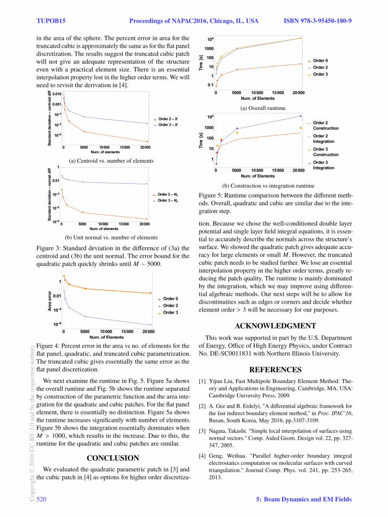
in the area of the sphere. The percent error in area for the

truncated cubic is approximately the same as for the flat panel

discretization. The results suggest the truncated cubic patch

will not give an adequate representation of the structure

even with a practical element size. There is an essential

interpolation property lost in the higher order terms. We will

need to revisit the derivation in [4].

(a) Centroid vs. number of elements

(b) Unit normal vs. number of elements

Figure 3: Standard deviation in the difference of (3a) the

centroid and (3b) the unit normal. The error bound for the

quadratic patch quickly shrinks until M ∼ 5000.

Figure 4: Percent error in the area vs no. of elements for the

flat panel, quadratic, and truncated cubic parametrization.

The truncated cubic gives essentially the same error as the

flat panel discretization.

We next examine the runtime in Fig. 5. Figure 5a shows

the overall runtime and Fig. 5b shows the runtime separated

by construction of the parametric function and the area inte-

gration for the quadratic and cubic patches. For the flat panel

element, there is essentially no distinction. Figure 5a shows

the runtime increases significantly with number of elements.

Figure 5b shows the integration essentially dominates when

M > 1000, which results in the increase. Due to this, the

runtime for the quadratic and cubic patches are similar.

CONCLUSION

We evaluated the quadratic parametric patch in [3] and

the cubic patch in [4] as options for higher order discretiza-

(a) Overall runtime

(b) Construction vs integration runtime

Figure 5: Runtime comparison between the different meth-

ods. Overall, quadratic and cubic are similar due to the inte-

gration step.

tion. Because we chose the well-conditioned double layer

potential and single layer field integral equations, it is essen-

tial to accurately describe the normals across the structure’s

surface. We showed the quadratic patch gives adequate accu-

racy for large elements or small M . However, the truncated

cubic patch needs to be studied further. We lose an essential

interpolation property in the higher order terms, greatly re-

ducing the patch quality. The runtime is mainly dominated

by the integration, which we may improve using differen-

tial algebraic methods. Our next steps will be to allow for

discontinuities such as edges or corners and decide whether

element order > 3 will be necessary for our purposes.

ACKNOWLEDGMENT

This work was supported in part by the U.S. Department

of Energy, Office of High Energy Physics, under Contract

No. DE-SC0011831 with Northern Illinois University.

REFERENCES

[1] Yijun Liu, Fast Multipole Boundary Element Method: The-

ory and Applications in Engineering, Cambridge, MA, USA:

Cambridge University Press, 2009.

[2] A. Gee and B. Erdelyi, "A differential algebraic framework for

the fast indirect boundary element method," in Proc. IPAC’16,

Busan, South Korea, May 2016, pp.3107-3109.

[3] Nagata, Takashi. "Simple local interpolation of surfaces using

normal vectors." Comp. Aided Geom. Design vol. 22, pp. 327-

347, 2005.

[4] Geng, Weihua. "Parallel higher-order boundary integral

electrostatics computation on molecular surfaces with curved

triangulation." Journal Comp. Phys. vol. 241, pp. 253-265,

2013.

TUPOB15 Proceedings of NAPAC2016, Chicago, IL, USA ISBN 978-3-95450-180-9

520Copy

right

©20

16CC

-BY-

3.0

and

byth

ere

spec

tive

auth

ors

5: Beam Dynamics and EM Fields