Embed Size (px)
Citation preview
Minerals 2018, 8, 443; doi:10.3390/min8100443 www.mdpi.com/journal/minerals
Article
Implicit 3D Modeling of Ore Body from Geological
Boreholes Data Using Hermite Radial Basis Functions
Jinmiao Wang 1,2, Hui Zhao 3, Lin Bi 1,2,* and Liguan Wang 1,2
1 School of Resources and Safety Engineering, Central South University, Changsha 410083, China;
[email protected] (J.W.); [email protected] (L.W.) 2 Digital Mine Research Center, Central South University, Changsha 410083, China 3 Faculty of Information Engineering, China University of Geosciences, Wuhan 430000, China;
* Correspondence: [email protected]; Tel.: +86-731-8887-7665 (ext. 8002)
Received: 3 September 2018; Accepted: 8 October 2018; Published: 10 October 2018
Abstract: Modeling ore body in 3D is the basis of digital intelligent mining. However, most existing
three-dimensional mining software uses the contour approach that requires too much man–machine
interaction and difficult partial updating. Moreover, accounting for uncertainty and low geometric
quality picking is very difficult in the direct contour approach. Therefore, an implicit modeling
approach to automatically build the three-dimensional model for ore body by means of spatial
interpolation directly based on the geological borehole data with Hermite radial basis function
(HRBF) algorithm as the core is proposed. Furthermore, in order to solve the problems of weak
continuity of models due to the long-distance original boreholes as well as the boundary-point
normal solution error, the densification of original borehole data with the virtual borehole as well
as the calculation of point-cloud normal direction based on the adjacent hole-drilling method is
proposed. The verification of two mine engineering projects and comparison with the explicit
modeling results show that this approach could realize the automatic building of three-dimensional
models for the ore body with high geometric quality, timely update and accurate results.
Keywords: discrete models; hermite interpolation; virtual borehole; marching cubes; Householder-QR
decomposition
1. Introduction
With the rising of “artificial intelligence” technology, the mining industry is paying more and
more attention to intelligent mining. In this framework, a preliminary step to intelligent mining is the
automatic building and quick updating of mineral resource models. However, for the existing three-
dimensional mining software (e.g., Vulcan, Datamine, Surpac, MineSight, Micromine, Dimine,
QuantyMine, 3Dmine, etc.), the contour tiling approach is generally adopted for the three-
dimensional model building for ore body. For this approach, there is much man–machine interaction,
low efficiency, low geometric quality, difficult partial update and other problems, which make it
difficult to satisfy the actual mine production demands [1]. Only rare mining software (e.g.,
SKUA/Gocad, Mira Suite, GeoModeler) offer implicit modeling facility since more than 10 years.
For implicit modeling, based on the geological exploration data processing in combination with
actual engineering demands, corresponding spatial interpolation function is selected to establish the
implicit equation of a surface to represent the geometrical morphology and grade distribution of the
ore body and the surface model pick-up algorithm is introduced for its drawing [2–6]. For implicit
modeling, there is no much man–machine interaction; moreover, due to a high degree of modeling

Minerals 2018, 8, 443 2 of 15
automatization and quick partial update, it is getting more and more wide attention in the field of
three-dimensional modeling for ore body.
For the common implicit modeling methods, there is the triangulation with linear interpolation
[7], nearest neighbor [8], distance power inverse ratio method [9], linear interpolation [10], local
polynomial [11], interpolation of radial basis function [12], spline interpolation [13], ordinary Kriging
[14], indicator Kriging [15], universal Kriging [16], etc. Implicit modeling methods have been focused
on and studied in the fields of digital terrain modeling [17,18], geological structure modeling [19,20],
reservoir modeling [21], hydrogeological modeling [22] and ore body modeling [23–25], etc. Among
them, three-dimensional implicit modeling of the ore body has become a research hotspot of mining
scholars all over the world in recent years. For example, Mallet [23] proposed a geological modeling
based on the discrete smooth interpolation algorithm, which is often applied to the stratified geologic
body modeling. Therefore, there are certain limitations in the application scenarios. Calcagno et al.
[24] proposed the potential field method for three-dimensional geologic modeling and the universal
Co-Kriging method to solve the interface between different rock stratums. Under the rock stratum
constraints, the Kriging interpolation is used for the ore body modeling. However, this method needs
interpretation based on original data in practical use. Moreover, the complex algorithm, heavy
calculation burden and weak geometric domain constraint result in considerable difference between
the ore body distribution and the actual morphology. Jiateng et al. [25] adopted the Hermite
interpolation method and Marching Cubes (MC) algorithm to build the implicit surface model, where
the radial basis function is used as the kernel function. However, for this method, the unit vector
pointing to high grade in the drilling direction is directly taken as the normal direction of the
boundary point, which is inaccurate. Because the shape of the ore body is extremely complex or
extremely irregular, the borehole cannot be exactly perpendicular to the ore body. Moreover, in view
of the sparse and scattered geological drilling, the implicit model built directly with this method
presents problems such as weak continuity and boundary closure failure. Therefore, despite the
fruitful research findings, there are still the following defects in the selection of algorithms and
solution: (1) It is hard for the implicit modeling algorithm to satisfy the modeling of various complex
ore bodies, i.e., this algorithm lacks general applicability; (2) There is high degree of algorithm
complexity, heavy calculation burden and slow solving speed; (3) For the implicit model built based
on the original geological borehole data, there are problems such as weak continuity and boundary
closure failure; and (4) The point-cloud normal solution is inaccurate.
Therefore, this paper takes the Hermite radial basis function algorithm as the core, which can
better meet the construction of implicit surface of the ore body with various complex topological
structures and geometric features. Secondly, the virtual borehole densification is used to improve the
borehole data intensity, which can solve the problems of poor continuity and non-closure of the
boundary of ore body model easily caused by sparse original geological boreholes. In addition, the
calculation of point-cloud normal direction based on the adjacent hole-drilling method is proposed to
ensure the accuracy of the point-cloud normal direction, and the inaccurate problem of the point cloud
normal solution is solved. Moreover, the least-squares Householder-QR decomposition method is
adopted to solve the HRBF coefficient matrix to improve the solving speed and solve the problem that
the algorithm complexity is high and the calculation amount is large, which causes the solution speed
to be slow. Finally, the Marching Cubes (MC) algorithm is introduced for the discretization of model
space and the iso-surface is extracted to realize the visualization of the implicit surface, so as to
ultimately realize the accurate building of three-dimensional model for complex ore body.
2. Hermite Radial Basis Function Principle
The radial basis function (RBF) interpolation only requires sampling point coordinates, and the
shape of the surface is controlled by adding the zero points on the surface and the constraint points
inside and outside the surface. However, it is hard to determine the distance from the constraint
points inside and outside the surface to the surface. Moreover, the shape of the surface is usually
extremely complicated, and it is easy to cause the cross phenomenon. Therefore, Macedo et al. [26–28]
combined the Hermite interpolation theory with the radial basis function and proposed the Hermite
Minerals 2018, 8, 443 3 of 15
radial basis function (HRBF) implicit surface building method, the core concept of which is to build an
implicit function and enable it to interpolate the position and normal direction of the sampling point.
The mathematical formulation of HRBF surface reconstruction algorithm is given as follows: For
the given sampling point set {(𝒙𝒊, 𝒏𝒊)|𝑖=1𝑁 }, where xi represents the position of the sampling point and
ni represents the normal direction of the sampling point, the constructor function f: R3→R meets the
following conditions:
{𝑓(𝒙𝒊) = 0
∇𝑓(𝒙𝒊) = 𝒏𝒊 (1)
Suppose function f(x) is a series of base functions by means of linear combination:
𝑓(𝒙) = ∑ 𝛼𝑖𝑘(𝒙𝒊, 𝒙)
𝑛
𝑖=1
(2)
In combination with Equation (1), this system is regularized in accordance with the optimization
theory:
𝐸(𝑓) = ‖𝑓‖𝐻2 +
𝐶1
𝑛∑ 𝑓(𝒙𝒊)
2
𝑛
𝑖=1
−𝐶2
𝑛∑⟨𝒏𝒊, ∇𝑓(𝒙𝒊)⟩
𝑛
𝑖=1
(3)
In Equation(3), C1 > 0 and C2 > 0 are weights used to account for fitting errors wit samples (f(xi)),
and measures errors from imposed gradient directions parallel to the normal; 𝑓(𝒙𝒊)2 is the coefficient
to measure the fitting degree of the function to the sampling point; < 𝒏𝒊, ∇𝑓(𝒙𝒊) > is to measure the
fitting degree of the function gradient to the normal direction of the sampling point; ‖𝑓‖𝐻 is the
regularization term of the function, and the smaller the value is, the smoother the surface will be; and
H is the reproducing Hilbert space of the kernel function. According to the derivation of Steinke et
al. [29], with the minimum E(f) and ∂E(f)/∂f = 0, there is:
𝑓(𝒙) = ∑{𝛼𝑖𝑘(𝒙𝒊, 𝒙) + ⟨𝜷𝒊, ∇𝑘(𝒙𝒊, 𝒙)⟩}
𝑛
𝑖=1
(4)
where 𝛼𝑖 = −𝐶1
𝑛𝑓(𝒙𝒊),𝜷𝒊 =
𝐶2
2𝑛𝒏𝒊.
In order to guarantee the positive definiteness of the solving system as well as the continuity of
the surface, one first-order polynomial is generally added, i.e.,
𝑓(𝒙) = ∑[𝛼𝑖𝑘(𝒙𝒊, 𝒙) + ⟨𝜷𝒊, ∇𝑘(𝒙𝒊, 𝒙)⟩]
𝑛
𝑖=1
+ 𝑝(𝒙) (5)
At this point, additional constraint conditions are needed for the one-first polynomial:
∑[𝛼𝑖𝑝𝑘(𝒙𝒊) + ⟨𝜷𝒊, ∇𝑝𝑘(𝒙𝒊)⟩]
𝑛
𝑖=1
= 0, 𝑘 = 1, 2, 3, 4 (6)
During the three-dimensional surface reconstruction, the radial basis function ensures
satisfactory point cloud data processing results, with high algorithm robustness, few independent
variables and high-order continuity, being applicable to the multivariate scattered and sparse data.
Therefore, the radial basis function is used for the kernel function. According to Equation (1), this
solving system is:
∑ [𝜑(𝒙𝒊 − 𝒙𝒋) ∇𝜑(𝒙𝒊 − 𝒙𝒋)
∇𝜑(𝒙𝒊 − 𝒙𝒋) 𝐻𝜑(𝒙𝒊 − 𝒙𝒋)] [
𝛼𝑗
𝜷𝒋]
𝑛
𝑗=1
+ ∑ 𝛾𝑘 [𝑝𝑘(𝒙𝒊)
∇𝑝𝑘(𝒙𝒊)]
4
𝑘=1
= [0𝒏𝒊
]
∑ [𝑝𝑘(𝒙𝒋) ∇𝑝𝑘(𝒙𝒋)𝑇
] [𝛼𝑗
𝜷𝒋]
𝑛
𝑗=1
= 0, 𝑖 = 1,2, … , 𝑛
(7)
Based on the sampling point set {(𝒙𝒊, 𝒏𝒊)|𝑖=1𝑁 }, αi, βi as well as γ (the coefficient of the first-order
polynomial) are obtained by establishing the linear system of equations in accordance with the above-

Minerals 2018, 8, 443 4 of 15
mentioned method. They are put in Equation (5) to obtain the implicit function f(x) for the surface
where the characterization sampling point set is.
This algorithm presents the advantages of the radial basis function in the implicit surface
building, being applicable to the description of sparse and non-uniform sampling surface and
guaranteeing satisfactory fitting of the surface with complex topological structure as well as
geometrical characteristics. Meanwhile, for this algorithm, the implicit function gradient being equal to
the normal vector of the sampling point is taken as the constraint condition and there is no need to
choose the offset distance. However, it also has disadvantages, such as discontinuity of derivatives at
the border of the neighborhood, and only deterministic solution, not possible to account for uncertainty.
3. Implicit Modeling Approach and Process
For the three-dimensional implicit modeling approach for ore body based on the geological
borehole data proposed in this paper, with the geological borehole data as the basis, the position and
depth of the virtual borehole as well as the sample length is determined based on the Delaunay
triangulation; the virtual borehole containing the mineral and rock information is determined based
on the Support Vector Machine (SVM); the borehole data are subject to sample length combination
to form the ore block based on the cut-off grade, minimum mining thickness, band rejected thickness
as well as the “low-grade ore to the delineation of ore body” thought; the upper-lower demarcation
point (i.e., the boundary point, referring to the mineral and rock demarcation point under the
minimum cut-off grade requirements) of each ore block is extracted and the normal direction of the
boundary point is calculated with the adjacent hole-drilling method, so as to obtain the Hermite point
cloud data set; the HRBF method is introduced for interpolation and accelerating the solving process
to obtain the implicit surface of the ore body model; and the MC algorithm is introduced for the
discretization of the model space and the iso-surface is extracted to finally realize the visualization of
the implicit surface of the ore body. More details are given as follows (Figure 1).
Figure 1. Three-dimensional Implicit Modeling Approach and Process for Ore Body.
(1) Based on the borehole position given by the original geological borehole data, the position of
the virtual borehole is obtained with the Delaunay triangulation; the depth and sample length of the
virtual borehole is determined based on that of the existing geological borehole; and the midpoint of
each sample length is extracted.
(2) The midpoint of each sample length in compliance with the cut-off grade in the original
geological borehole data is extracted, and is used to the SVM training and testing, so as to obtain the
optimal classification function to predict the mineral and rock information of each sample length of
the virtual borehole. The detailed determination method is given in Section 4 of this paper.
(3) The geological borehole data and the virtual borehole data constitute the borehole database;
the borehole data are subject to sample length combination to form the ore block based on the cut-off
grade, minimum mining thickness, band rejected thickness as well as the “low-grade ore to the
delineation of ore body” thought; and the upper-lower demarcation point, i.e., the boundary point,
of each ore block is extracted.
(4) Based on the boundary point so obtained as well as its corresponding borehole, the neighbour
borehole of each borehole as well as its corresponding boundary point is obtained with the Delaunay
Minerals 2018, 8, 443 5 of 15
triangulation; and the normal direction of such point is obtained with Principal Component Analysis
(PCA) method. The normal direction of the upper boundary point of some borehole can be obtained
by identifying the upper boundary point of its adjacent borehole with the PCA method. The detailed
solving process is given in Section 5 of this paper.
(5) The boundary points as well as their corresponding normal directions constitute the Hermite
point cloud data set; and the implicit function equation for the three-dimensional mode for ore body
is obtained through the interpolation approximation based on HRBF as well as accelerating the
solving process based on the least-squares Householder-QR decomposition method [30].
(6) The model space corresponding to the implicit function surface of the three-dimensional
model for ore body is discretized with the MC algorithm [31] and the vertex value of each cube
discretized is calculated to extract the iso-surface, so as to finally build the three-dimensional model
for the ore body.
(7) In case of any change in the cut-off grade or any new borehole data with the productive
exploration, the above (3)–(6) will be re-executed to quickly realize the update of the three-
dimensional model for the ore body.
4. Determination of the Virtual Borehole and Extraction of Its Boundary Point
For the geological borehole, there is high drilling cost and generally a long distance between two
boreholes. According to the mathematical features of kernel function in the HRBF algorithm, the
bigger the distance between two points is, the larger the kernel function value attenuation of the two
points will be. In this case, there will be scattered ore body, with weak continuity. Therefore, in order
to improve the continuity of the ore body model and ensure the accuracy of the ore body model, the
virtual borehole [32,33] are added between boreholes, i.e., the position of the virtual borehole is
determined with the Delaunay triangulation based on the original geological borehole and the
mineral and rock information on the virtual borehole is obtained with the SVM classification method.
4.1. SVM Principle
The SVM (Support Vector Machines) [34–36] mechanism is to find the optimal separating
hyperplane in the sample characteristic space which not only meets the classification accuracy
requirement, but also maximizes the classification interval. The optimal separating hyperplane so
obtained is used to predict the unknown data.
The separating hyperplane is expressed as 𝒘𝑇𝑥 + 𝑏 = 0 (w and b is respectively the normal
vector and offset of the hyperplane). Suppose the given data set is {(𝒙𝟏, 𝑦1), (𝒙𝟐, 𝑦2), ⋯ , (𝒙𝒏, 𝑦𝑛)},𝒙 ∈
space 𝑅𝑑,𝑦 ∈ {−1, +1} , map the data from the low-dimensional sample space Rd to the high-
dimensional characteristic space H, i.e., 𝒙𝒊 → 𝜑(𝒙𝒋) , choose a proper kernel function to make
𝑘(𝒙𝒊, 𝒙𝒋) = 𝜑(𝒙𝒊) ∙ 𝜑(𝒙𝒋), and introduce the slack variable 𝜉1, 𝜉2, ⋯ , 𝜉𝑛 and penalty factor C.
For the SVM solution, the Lagrangian multiplier 𝛼1, 𝛼2, ⋯ , 𝛼𝑛 as well as 𝜇1, 𝜇2, ⋯ , 𝜇𝑛 is
introduced to establish the Lagrangian function and transform the original convex quadratic
programming problem into the dual problem, obtaining the optimal 𝛼∗ = (𝛼1∗, 𝛼2
∗, ⋯ , 𝛼𝑛∗ ) and the
support vector S={i∣αi > 0,i = 1, 2, …, n} in the original sample set. The optimal weight vector 𝒘∗ =
∑ 𝛼𝑖∗𝑦𝑖𝒙𝒊𝑖∈𝑆 and the optimal offset 𝑏∗ =
1
|𝑆|∑ (𝑦𝑠 − ∑ 𝛼𝑖
∗𝑦𝑖𝑘(𝒙𝒊, 𝒙𝒔𝑖∈𝑆 )𝑠∈𝑆 ) are calculated. The optimal
classification function is finally given as follows:
𝑓(𝑥) = 𝑠𝑖𝑔𝑛 {[∑ 𝛼𝑖∗𝑦𝑖𝑘(𝒙𝒊, 𝒙𝒔
𝑖∈𝑆
)] + 𝑏∗} (8)
4.2. Determination of the Optimal Classification Function
(1) Determination of the Borehole Position
For the determination of the borehole position, the position of each original geological borehole
is mapped onto the XY plane; the two-dimensional borehole point mapped onto the XY plane is
Minerals 2018, 8, 443 6 of 15
subject to the Delaunay triangulation and the borehole index is established based on the structured
grid relationship; after each triangular patch in the above Delaunay grid is traversed, the borehole
positions corresponding to the three vertexes of the existing triangular patches are extracted. The position
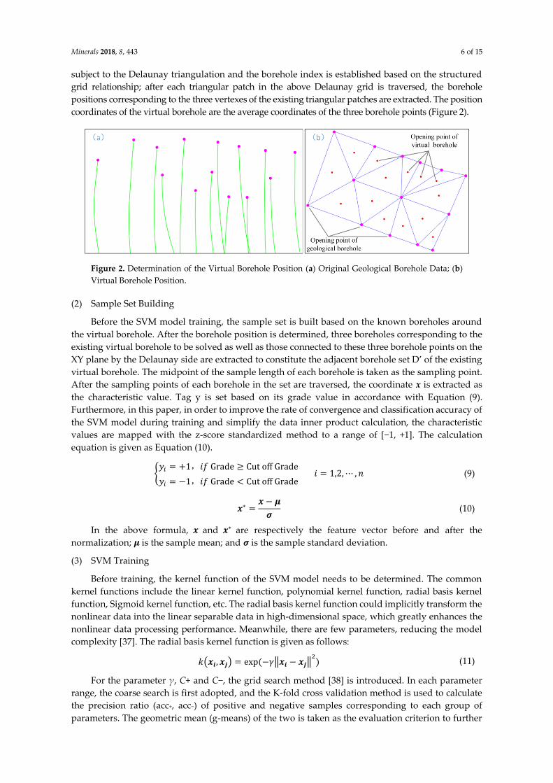
coordinates of the virtual borehole are the average coordinates of the three borehole points (Figure 2).
Figure 2. Determination of the Virtual Borehole Position (a) Original Geological Borehole Data; (b)
Virtual Borehole Position.
(2) Sample Set Building
Before the SVM model training, the sample set is built based on the known boreholes around
the virtual borehole. After the borehole position is determined, three boreholes corresponding to the
existing virtual borehole to be solved as well as those connected to these three borehole points on the
XY plane by the Delaunay side are extracted to constitute the adjacent borehole set D’ of the existing
virtual borehole. The midpoint of the sample length of each borehole is taken as the sampling point.
After the sampling points of each borehole in the set are traversed, the coordinate x is extracted as
the characteristic value. Tag y is set based on its grade value in accordance with Equation (9).
Furthermore, in this paper, in order to improve the rate of convergence and classification accuracy of
the SVM model during training and simplify the data inner product calculation, the characteristic
values are mapped with the z-score standardized method to a range of [−1, +1]. The calculation
equation is given as Equation (10).
{𝑦𝑖 = +1,𝑖𝑓 Grade ≥ Cut off Grade
𝑦𝑖 = −1,𝑖𝑓 Grade < Cut off Grade 𝑖 = 1,2, ⋯ , 𝑛 (9)
𝒙∗ =𝒙 − 𝝁
𝝈 (10)
In the above formula, 𝒙 and 𝒙∗ are respectively the feature vector before and after the
normalization; 𝝁 is the sample mean; and 𝝈 is the sample standard deviation.
(3) SVM Training
Before training, the kernel function of the SVM model needs to be determined. The common
kernel functions include the linear kernel function, polynomial kernel function, radial basis kernel
function, Sigmoid kernel function, etc. The radial basis kernel function could implicitly transform the
nonlinear data into the linear separable data in high-dimensional space, which greatly enhances the
nonlinear data processing performance. Meanwhile, there are few parameters, reducing the model
complexity [37]. The radial basis kernel function is given as follows:
𝑘(𝒙𝒊, 𝒙𝒋) = exp (−𝛾‖𝒙𝒊 − 𝒙𝒋‖2
) (11)
For the parameter γ, C+ and C−, the grid search method [38] is introduced. In each parameter
range, the coarse search is first adopted, and the K-fold cross validation method is used to calculate
the precision ratio (acc+, acc−) of positive and negative samples corresponding to each group of
parameters. The geometric mean (g-means) of the two is taken as the evaluation criterion to further

Minerals 2018, 8, 443 7 of 15
determine the local optimal parameter. The fine search is then adopted within the surrounding area
to solve the optimal classification forecasting function.
𝑎𝑐𝑐+ =𝑡𝑟𝑢𝑒 𝑝𝑜𝑠𝑖𝑡𝑖𝑣𝑒
𝑡𝑜𝑡𝑎𝑙 𝑝𝑜𝑠𝑖𝑡𝑖𝑣𝑒
𝑎𝑐𝑐− =𝑡𝑟𝑢𝑒 𝑛𝑒𝑔𝑎𝑡𝑖𝑣𝑒
𝑡𝑜𝑡𝑎𝑙 𝑛𝑒𝑔𝑎𝑡𝑖𝑣𝑒
𝑔 − 𝑚𝑒𝑎𝑛𝑠 = √𝑎𝑐𝑐+ · 𝑎𝑐𝑐−
(12)
4.3. Determination of the Virtual Borehole and Extraction of the Boundary Point
The mineral and rock information of each sample length of the existing virtual borehole is
predicted in accordance with the optimal classification function solved in Section 4.2 and the sample
lengths are combined to form the ore block before the boundary point of each ore block is extracted.
The detailed process is given as follows:
(1) Suppose the existing virtual borehole point coordinate is 𝒑𝟎 = (𝑥𝑖 , 𝑦𝑖 , 𝑧𝑖), the maximum hole
depth is h and the sample length is l.
(2) Extract the midpoint of all sample lengths of the virtual borehole as the predicted sampling point
in accordance with Equation (13), constituting the sampling point set to be measured P.
𝒑𝒊 = {(𝑥𝑖 , 𝑦𝑖 , 𝑧𝑖 + (𝑡 +1
2) ∗ 𝑙) |𝑧𝑖 + (𝑡 +
1
2) ∗ 𝑙 < ℎ, 𝑡 = 0,1,2, ⋯ , 𝑛} (13)
where pi is the midpoint coordinate of the sample length of the i-th segment; n is a natural number.
(3) Calculate the function value of each point in the point set P based on the optimal function solved. If
less than 0, the point indicates rock, written as −1; otherwise, it indicates mineral, written as +1.
(4) Rank the points in the point set P from biggest to smallest in accordance with the Z coordinate
value and combine the sample lengths of which the point is written as +1 to form the ore block
in accordance with the constraint conditions, such as the minimum mining thickness and band
rejected thickness.
(5) Extract the upper-lower demarcation point, i.e., the boundary point, of each ore block of the
borehole to realize the extraction of the boundary point of the virtual borehole.
5. Point-Cloud Normal Vector Calculation
The normal direction information of the boundary point set is of vital importance for the implicit
modeling of the ore body. It is not only a basic element of the HRBF algorithm, but also one of the
important mediums for the control of the curved surface model. For surface reconstruction, the PCA
(Principal Component Analysis) [39] is generally adopted to calculate the point-cloud normal direction.
However, for this method, the dense and uniform point cloud is the precondition, while the geological
borehole is sparse and scattered, with a complex topological structure. Therefore, during the selection of
neighbourhood points, there is often confusion, leading to the normal solution error. Although it is
impossible to obtain the neighbourhood points with the conventional method, the borehole adjacent to
that where this boundary point is located may be determined. Between adjacent boreholes, the
corresponding neighbourhood points can be determined based on the corresponding relationship
between the upper and lower boundary points and then the normal direction can be determined.
Therefore, based on the PCA algorithm, this paper proposes the point-cloud normal direction calculation
method based on the adjacent borehole. More details are given as follows:
(1) The boundary point as well as the data set {D1, D2, …, Dl} of the corresponding borehole is given,
and the coordinates of opening point for each borehole is extracted and mapped onto the XY
two-dimensional plane.

Minerals 2018, 8, 443 8 of 15
(2) As shown in Figure 3, the two-dimensional borehole point is subject to the Delaunay
triangulation; all points connected to the existing borehole points by the Delaunay side are
defined as the neighbourhood points of the existing points and the corresponding borehole is
the neighbourhood borehole. The neighbourhood borehole search tree is therefore established
based on the structured grid relationship.
Figure 3. Diagram for the Neighborhood Borehole Solution.
(3) All boreholes in the data set are traversed. For the existing borehole Di, the neighbourhood
borehole set is {Dm}. As shown in Figure 4, each boundary point pj in the Di is traversed. If the
point is the upper boundary point, the upper boundary point of each borehole Dm in the
neighbourhood borehole set is extracted. If the number of the upper boundary points of Dm is n
> 1, the dip angle of the rock stratum or ore body obtained during exploration is taken as the
basis for the selection of the neighbourhood point, i.e., the boundary point pj is connected to each
upper boundary point of Dm and the included angle of their respective projection line on the
horizontal plane and the connection line to the boundary point is calculated. The upper
boundary point nearest to the dip angle of the rock stratum or ore body is selected as the
neighbourhood point of pj. When pj is the lower boundary point, it can be obtained in a similar
way. The neighbourhood point set {Ot} of each boundary point pj in the Di is therefore obtained.
Figure 4. Diagram for the Neighborhood Point Set Solution.

Minerals 2018, 8, 443 9 of 15
(4) As shown in Figure 5, two adjacent boundary points Oi and Oi+1 are taken from the {Ot} and the
local plane is solved based on the three points of {pj, Oi, Oi+1}, and finally the normal direction set
n of the local plane is obtained.
Figure 5. Normal Direction Solution of the Local Plane.
(5) The set for normal n is traversed. If the current normal direction is ni, the next is nj. If 𝒏𝒊 ∙ 𝒏𝒋 < 0,
nj is inverted.
(6) All normal averages in the set n are the normal N of pj.
6. Experiments and Results
The VC++ development tools are used for the secondary development on the DIMINE three-
dimensional mining software platform, with the experiment operating environment of Windows7,
CPU of Intel (R) Core (TM) i5-4590 [email protected] and memory of 8GB. The mine engineering cases I
and II are subject to the ore body modeling experiment. Figure 6 shows the borehole data of Case I
and Case II, including the geological borehole and virtual borehole, where the red line segment
represents the mineral that is higher than the cut-off grade and the green part represents the rock that
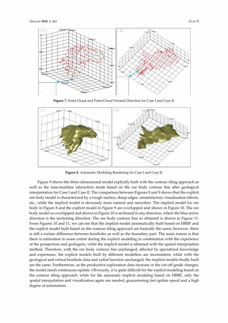
is lower than the cut-off grade. Figure 7 shows the boundary point cloud extracted based on the
borehole data for Case I and Case II as well as the point-cloud normal direction calculated based on the
adjacent borehole method, where the blue line represents the point-cloud normal direction. Figure 8
shows the automatic modeling rendering based on HRBF for Case I and Case II, respectively
including 101,465 and 7,982 triangular patches, with smooth and natural surface and high geometric
quality. For Case I and Case II, the solving time for the HRBF coefficient matrix based on the
Householder-QR decomposition is about 1s.
Figure 6. Borehole Data for Case I and Case II.
Minerals 2018, 8, 443 10 of 15
Figure 7. Point Cloud and Point-Cloud Normal Direction for Case I and Case II.
Figure 8. Automatic Modeling Rendering for Case I and Case II.
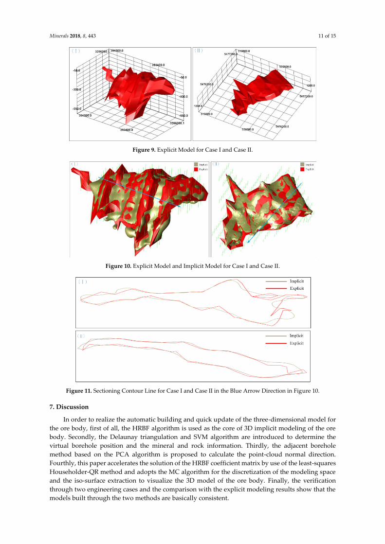
Figure 9 shows the three-dimensional model explicitly built with the contour tiling approach as
well as the man-machine interaction mode based on the ore body contour line after geological
interpretation for Case I and Case II. The comparison between Figures 8 and 9 shows that the explicit
ore body model is characterized by a rough surface, sharp edges, unsatisfactory visualization effects,
etc., while the implicit model is obviously more natural and smoother. The implicit model for ore
body in Figure 8 and the explicit model in Figure 9 are overlapped and shown in Figure 10. The ore
body model so overlapped and shown in Figure 10 is sectioned in any direction, where the blue arrow
direction is the sectioning direction. The ore body contour line so obtained is shown in Figure 11.
From Figures 10 and 11, we can see that the implicit model automatically built based on HRBF and
the explicit model built based on the contour tiling approach are basically the same; however, there
is still a certain difference between boreholes as well as the boundary part. The main reason is that
there is estimation to some extent during the explicit modeling in combination with the experience
of the prospectors and geologists, while the implicit model is obtained with the spatial interpolation
method. Therefore, with the ore body contour line unchanged, affected by specialized knowledge
and experience, the explicit models built by different modellers are inconsistent; while with the
geological and virtual borehole data and radial function unchanged, the implicit models finally built
are the same. Furthermore, as the productive exploration data increase or the cut-off grade changes,
the model needs continuous update. Obviously, it is quite difficult for the explicit modeling based on
the contour tiling approach, while for the automatic implicit modeling based on HRBF, only the
spatial interpolation and visualization again are needed, guaranteeing fast update speed and a high
degree of automation.
Minerals 2018, 8, 443 11 of 15
Figure 9. Explicit Model for Case I and Case II.
Figure 10. Explicit Model and Implicit Model for Case I and Case II.
Figure 11. Sectioning Contour Line for Case I and Case II in the Blue Arrow Direction in Figure 10.
7. Discussion
In order to realize the automatic building and quick update of the three-dimensional model for
the ore body, first of all, the HRBF algorithm is used as the core of 3D implicit modeling of the ore
body. Secondly, the Delaunay triangulation and SVM algorithm are introduced to determine the
virtual borehole position and the mineral and rock information. Thirdly, the adjacent borehole
method based on the PCA algorithm is proposed to calculate the point-cloud normal direction.
Fourthly, this paper accelerates the solution of the HRBF coefficient matrix by use of the least-squares
Householder-QR method and adopts the MC algorithm for the discretization of the modeling space
and the iso-surface extraction to visualize the 3D model of the ore body. Finally, the verification
through two engineering cases and the comparison with the explicit modeling results show that the
models built through the two methods are basically consistent.

Minerals 2018, 8, 443 12 of 15
Due to the sparse and scattered geological borehole data, the bigger the distance between the
boundary points of two adjacent boreholes is, the faster the attenuation of the kernel function value
in the HRBF will be. Especially for the ore body with the large fluctuation of the form or narrow vein,
there might be scattered distribution and weak continuity. Figure 12 shows an extremely thin ore
body area in the west (Case I). Figure 12a shows the point cloud as well as its normal direction,
indicating that the boundary point of the west is far away from the midpoint. The implicit model
built with the approach given in this paper is shown in Figure 12b, where the two isolated points
along the boundary are directly pinched out. The comparison between the explicit model built based
on the contour line and the implicit model built with the approach under this paper is shown in
Figure 12c. Therefore, in case of a bigger distance between the boundary points, a large fluctuation
of the form of the ore body, narrow vein, etc., the building of the ore body model with satisfactory
continuity and higher degree of accuracy requires the borehole data densification based on the
Delaunay and SVM algorithm.
Figure 12. Point Cloud along the Boundary of the Ore Body Area in the West and the Ore Body Model
(Case I). (a) Point Cloud and Point-Cloud Normal Direction. (b) Implicit Model built with
the Approach. (c) Comparison between the Explicit Model and Implicit Model.
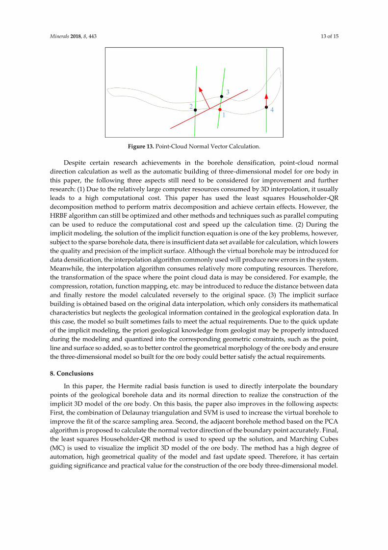
The solution of the implicit surface equation with the HRBF algorithm requires the solution of
the normal direction of the boundary point. However, the boundary points between the boreholes
are quite sparsely distributed. When the thickness of the ore body is smaller than the distance
between the boreholes, the traditional PCA method is used for solving, with the neighbourhood
points solved including the boundary points of the same borehole, which will lead to the normal
solution error. As shown in Figure 13, for the solution of the normal direction of Point 1, the PCA
method is introduced, with Point 2 and Point 3 selected as the neighbourhood points, and the normal
direction of Point 1 so obtained is roughly the red arrow direction in the middle of Point 1, Point 2
and Point 3, which is obviously incorrect. When solving the point-cloud normal direction, Jiateng et
al. [25] directly took the unit vector pointing to high grade in the drilling direction of the point as the
normal direction of this point (Point 4 in Figure 13). Obviously, it is incorrect to take the red arrow
direction at Point 4 as its normal direction. Therefore, based on the PCA algorithm, this paper
proposes the point-cloud normal vector calculation on the basis of the adjacent borehole. As shown
in Figure 13, for the solution of the normal direction of the Lower Boundary Point 1, the adjacent
borehole of the borehole where Point 1 is located may be first identified and then the Lower Boundary
Point 2 and 4 of the adjacent borehole may be correspondingly identified. Finally, the normal
direction of Point 1 can be accurately calculated.
Minerals 2018, 8, 443 13 of 15
Figure 13. Point-Cloud Normal Vector Calculation.
Despite certain research achievements in the borehole densification, point-cloud normal
direction calculation as well as the automatic building of three-dimensional model for ore body in
this paper, the following three aspects still need to be considered for improvement and further
research: (1) Due to the relatively large computer resources consumed by 3D interpolation, it usually
leads to a high computational cost. This paper has used the least squares Householder-QR
decomposition method to perform matrix decomposition and achieve certain effects. However, the
HRBF algorithm can still be optimized and other methods and techniques such as parallel computing
can be used to reduce the computational cost and speed up the calculation time. (2) During the
implicit modeling, the solution of the implicit function equation is one of the key problems, however,
subject to the sparse borehole data, there is insufficient data set available for calculation, which lowers
the quality and precision of the implicit surface. Although the virtual borehole may be introduced for
data densification, the interpolation algorithm commonly used will produce new errors in the system.
Meanwhile, the interpolation algorithm consumes relatively more computing resources. Therefore,
the transformation of the space where the point cloud data is may be considered. For example, the
compression, rotation, function mapping, etc. may be introduced to reduce the distance between data
and finally restore the model calculated reversely to the original space. (3) The implicit surface
building is obtained based on the original data interpolation, which only considers its mathematical
characteristics but neglects the geological information contained in the geological exploration data. In
this case, the model so built sometimes fails to meet the actual requirements. Due to the quick update
of the implicit modeling, the priori geological knowledge from geologist may be properly introduced
during the modeling and quantized into the corresponding geometric constraints, such as the point,
line and surface so added, so as to better control the geometrical morphology of the ore body and ensure
the three-dimensional model so built for the ore body could better satisfy the actual requirements.
8. Conclusions
In this paper, the Hermite radial basis function is used to directly interpolate the boundary
points of the geological borehole data and its normal direction to realize the construction of the
implicit 3D model of the ore body. On this basis, the paper also improves in the following aspects:
First, the combination of Delaunay triangulation and SVM is used to increase the virtual borehole to
improve the fit of the scarce sampling area. Second, the adjacent borehole method based on the PCA
algorithm is proposed to calculate the normal vector direction of the boundary point accurately. Final,
the least squares Householder-QR method is used to speed up the solution, and Marching Cubes
(MC) is used to visualize the implicit 3D model of the ore body. The method has a high degree of
automation, high geometrical quality of the model and fast update speed. Therefore, it has certain
guiding significance and practical value for the construction of the ore body three-dimensional model.

Minerals 2018, 8, 443 14 of 15
Author Contributions: J.W. and H.Z. came up with the main idea and wrote the manuscript; L.B. verified the
algorithm; L.W. analysed the data; all authors discussed the results and revised the paper.
Funding: This research was funded by the National Natural Science Foundation of China (41572317), the National
Key R&D Program of China (2017YFC0602905), the Fundamental Research Funds for the Central Universities of
Central South University (2017zzts189), and the National Natural Science Foundation of China (51604301).
Acknowledgments: Thanks to the following organizations who provided provide basis data and technique
support for this research: Changsha Digital Mine Co., Ltd., Dlib C++ Library and the Computational Geometry
Algorithms Library.
Conflicts of Interest: The authors declare no conflict of interest.
References
1. Lin, B.; Xiaoming, L.; Xin, C.; Zhonghua, Z. An automatic 3D modeling method based on orebody contours.
Geomat. Inf. Sci. Wuhan Univ. 2016, 41, 1359–1365. (In Chinese)
2. Yanhong, Z.; Jianchun, H. A spatial shape simulation method for three-dimensional geological body based
on marching cubes algorithm. Acta Geod. Cartogr. Sin. 2012, 41, 910–917.
3. Morse, B.S.; Yoo, T.S.; Rheingans, P.; Chen, D.T.; Subramanian, K.R. Interpolating implicit surfaces from
scattered surface data using compactly supported radial basis functions. In Proceedings of the International
Conference on Shape Modeling Application, Washington, DC, USA, 7–11 May 2001; pp. 89–98.
4. McInerney, P.; Goldberg, A.; Calcagno, P.; Courrioux, G.; Guillen, R.; Seikel, R. An improved 3D geology
modelling using an implicit function interpolator and forward modelling of potential field data. In
Proceedings of the Exploration 07: Fifth Decennial International Conference on Mineral Exploration,
Toronto, ON, Canada, 2007; pp. 919–922.
5. Laurent, G.; Ailleres, L.; Grose, L.; Caumon, G.; Jessell, M.; Armit, R. Implicit modeling of folds and
overprinting deformation. Earth Planet. Sci. Lett. 2016, 456, 26–38.
6. Clausolles, N.; Collon, P.; Caumon, G. A workflow for 3D stochastic modeling of salt from seismic images.
In Proceedings of the 80th EAGE Conference and Exhibition 2018, Copenhagen, Denmark, 11–14 June 2018.
7. Dyn, N.; Levin, D.; Rippa, S. Data dependent triangulations for piecewise linear interpolation. IMA J.
Numer. Anal. 1990, 10, 137–154.
8. Olivier, R.; Hanqiang, C. Nearest neighbor value interpolation. IJACSA 2012, 3, 1–6.
9. Lu, G.Y.; Wong, D.W. An adaptive inverse-distance weighting spatial interpolation technique. Comput.
Geosci. 2008, 34, 1044–1055.
10. Powell, M.J. A Direct Search Optimization Method that Models the Objective and Constraint Functions by Linear
Interpolation; Springer: Dordrecht, The Netherlands, 1994; pp. 51–67.
11. Baker, K.A.; Pixley, A.F. Polynomial interpolation and the Chinese remainder theorem for algebraic
systems. Math. Z. 1975, 143, 165–174.
12. Broomhead, D.S.; Lowe, D. Radial Basis Functions, Multi-Variable Functional Interpolation and Adaptive
Networks; Royal Signals and Radar Establishment: Malvern, UK, 1988.
13. De Boor, C.; De Boor, C.; Mathématicien, E.-U.; De Boor, C.; De Boor, C. A practical Guide to Splines; Springer:
New York, NY, USA, 1978; p. 27.
14. Cressie, N. Spatial prediction and ordinary kriging. Math. Geol. 1988, 20, 405–421.
15. Marinoni, O. Improving geological models using a combined ordinary–indicator kriging approach. Eng.
Geol. 2003, 69, 37–45.
16. Zimmerman, D.; Pavlik, C.; Ruggles, A.; Armstrong, M.P. An experimental comparison of ordinary and
universal kriging and inverse distance weighting. Math. Geol. 1999, 31, 375–390.
17. Cichocinski, P.; Basista, I. The comparison of spatial interpolation methods in application to the
construction of digital terrain models. In Proceedings of the Geoconference on Informatics, Geoinformatics
and Remote Sensing, Albena, Bulgaria, 2013; pp. 959–966.
18. Gosciewski, D. Reduction of deformations of the digital terrain model by merging interpolation algorithms.
Comput. Geosci. 2014, 64, 61–71.
19. Irakarama, M.; Laurent, G.; Renaudeau, J.; Caumon, G. Finite difference implicit modeling of geological
structures. In Proceedings of the 80th EAGE Conference and Exhibition 2018, Copenhagen, Denmark, 2018.
20. Grose, L.; Laurent, G.; Aillères, L.; Armit, R.; Jessell, M.; Caumon, G. Structural data constraints for implicit
modeling of folds. J. Struct. Geol. 2017, 104, 80–92.
Minerals 2018, 8, 443 15 of 15
21. Cao, R.; Ma, Y.Z.; Gomez, E. Geostatistical applications in petroleum reservoir modelling. J. South. Afr. Inst.
Min. Metall. 2014, 114, 625–629.
22. Aoki, K.; Mito, Y. Hydrogeological Modelling of Rock Mass by Mds-Idw Technique; CRCPress/Balkema: Leiden,
The Netherlands, 2006; pp. 677–682
23. Mallet, J.L. Discrete smooth interpolation in geometric modelling. Comput. Aided Des 1992, 24, 178–191.
24. Calcagno, P.; Chilès, J.P.; Courrioux, G.; Guillen, A. Geological modelling from field data and geological
knowledge. Phys. Earth Planet. Inter. 2008, 171, 147–157.
25. Jiateng, G.; Lixin, W.; Wenhui, Z. Automatic ore body implicit 3d modeling based on radial basis function
surface. J. China Coal Soc. 2016, 41, 2130–2135.
26. Macêdo, I.; Gois, J.P.; Velho, L. Hermite interpolation of implicit surfaces with radial basis functions. In
Proceedings of the XXII Brazilian Symposium on Computer Graphics and Image Processing, Rio de Janiero,
Brazil, 11–15 October 2009; pp. 1–8.
27. Macêdo, I.; Gois, J.P.; Velho, L. Hermite radial basis functions implicits. Comput. Gr. Forum 2011, 30, 27–42.
28. Brazil, E.; Macedo, I.; Sousa, M.C.; de Figueiredo, L.H.; Velho, L. Sketching variational hermite-rbf
implicits. In Proceedings of the Seventh Sketch-Based Interfaces and Modeling Symposium, Annecy,
France, 7–10 June 2010; pp. 1–8.
29. Steinke, F.; Schölkopf, B. Kernels, regularization and differential equations. Pattern Recognit. 2008, 41, 3271–
3286.
30. Cox, A.J.; Higham, N.J. Stability of householder qr factorization for weighted least squares problems. In
Numerical Analysis; CRC Press: Boca Raton, FL, USA, 1997.
31. Lorensen, W.E.; Cline, H.E. Marching cubes: A high resolution 3D surface construction algorithm. In
Proceedings of the 14th Annual Conference on Computer Graphics and Interactive Techniques, Boulder,
Co, USA, 1987; pp 163–169.
32. Wang, G.; Huang, L. 3D geological modeling for mineral resource assessment of the tongshan cu deposit,
Heilongjiang province, China. Geosci. Front. 2012, 3, 483–491.
33. Wang, G.; Du, Y.; Cui, G.; Tan, C. Mineral resource prediction based on 3D-GIS and BP network technology:
A case of study in pulang copper deposit, Yunnan province, China. Nat. Comput. 2009, 3, 382–386.
34. Hearst, M.A.; Dumais, S.T.; Osuna, E.; Platt, J.; Scholkopf, B. Support vector machines. IEEE Intell. Syst.
Appl. 1998, 13, 18–28.
35. An, Y.; Ding, S.; Shi, S.; Li, J. Discrete space reinforcement learning algorithm based on support vector
machine classification. Pattern Recognit. Lett. 2018, 111, 30–35.
36. Ding, S.; Qi, B.J.; Tan, H.Y. An. overview on theory and algorithm of support vector machines. J. Univ.
Electron. Sci. Technol. China 2011, 40, 2–10.
37. Han, S.; Cao, Q.; Han, M. Parameter selection in SVM with RBF kernel function. In Proceedings of the
World Automation Congress, Puerto Vallarta, Mexico, 24–28 June 2012; pp. 1–4.
38. Bao, Y.; Liu, Z. A Fast Grid Search Method in Support Vector Regression Forecasting Time Series; Springer: Berlin,
Germany, 2006; pp. 504–511.
39. Jolliffe, I. Principal component analysis. In International Encyclopedia of Statistical Science; Lovric, M., Ed.;
Springer: Berlin, Germany, 2011; pp. 1094–1096.
© 2018 by the authors. Licensee MDPI, Basel, Switzerland. This article is an open access
article distributed under the terms and conditions of the Creative Commons Attribution
(CC BY) license (http://creativecommons.org/licenses/by/4.0/).