Importance of Regional Rainfall Data inHomogeneous Clustering of Data Sparse Areas: AStudy in the Upper Brahmaputra Valley RegionJayshree Hazarika  ( jayshree@iitg.ac.in )

Assam Engineering College https://orcid.org/0000-0002-7155-8752Arup Kumar Sarma 

Indian Institute of Technology Guwahati

Research Article

Keywords: Regionalization, L-moments, Fuzzy clustering, Homogeneity test

Posted Date: April 15th, 2021

DOI: https://doi.org/10.21203/rs.3.rs-349940/v1

License: This work is licensed under a Creative Commons Attribution 4.0 International License.  Read Full License

1

Importance of Regional Rainfall Data in Homogeneous Clustering of Data 1

Sparse Areas: A Study in the Upper Brahmaputra Valley Region 2

Jayshree Hazarika1,2, Arup Kumar Sarma1 3

1Department of Civil Engineering, Indian Institute of Technology Guwahati, Guwahati – 4

781039, Assam, India 5

2Department of Civil Engineering, Assam Engineering College, Guwahati – 781013, Assam, 6

India 7

Corresponding Author: Dr. Jayshree Hazarika 8

Email ID: jayshree@iitg.ac.in; ORCID ID: 0000-0002-7155-8752 9

Abstract 10

Delineation of homogeneous regions has found its way into many hydrological applications as 11

it helps in addressing the challenges in understanding the behavior of rainfall distribution and 12

its variability at a local scale. In the present study, rainfall data recoded by 83 tea gardens in 13

the upper Brahmaputra valley region of Assam have been used to identify homogeneous 14

rainfall regions by using fuzzy clustering analysis. Further, seven different cluster validity 15

indices (CVs) were utilized to find out the optimum clustering in the fuzzy c-means (FCM) 16

algorithm. The clusters thus formed were assessed for statistical homogeneity by performing 17

homogeneity tests based on L-moment. Three different combinations of feature vectors were 18

employed in FCM algorithm and the outputs were compared for attaining best solutions to 19

regionalization. The results were further compared with previous regionalization studies. The 20

analysis and comparison conclude that if regionalization needs to be done at a local scale, 21

further sub-clustering of a larger clustered region to smaller regions may be required. Local 22

rainfall data can be used for the purpose provided a good dataset with large number of station 23

points are available within the region. Along with rainfall data, geographical location 24

2

parameters (latitude, longitude and elevation) need to be taken into account for getting a 25

definite conclusion. 26

27

Keywords: 28

Regionalization, L-moments, Fuzzy clustering, Homogeneity test 29

30

3

1. Introduction 31

Rainfall is one of the most important hydrological parameters that requires to be studied 32

scrupulously, both in spatial and temporal scale. However, challenge comes in understanding 33

the behavior of rainfall distribution pattern when applied on a regional scale. Pattern of rainfall, 34

its frequency and magnitude may drastically vary depending upon the orography (Venkatesh 35

and Jose 2007), large-scale synoptic and convective precipitation types (Karaca et al. 2000, 36

Unal et al. 2012; Baltacı et al. 2015; Efe et al. 2019) of the region. Scarcity of sufficient data 37

at many sites of interest, may further complicate the investigation. To address this issue, the 38

region may be classified into few homogeneous rainfall regions of similar rainfall distribution, 39

also termed as regionalization. The Brahmaputra valley region is situated in the northeastern 40

part of India, that has its own peculiar topography. The variations in the orographic 41

arrangements and altitude differences in the region give rise to irregular and complex rainfall 42

patterns at a local scale, which eventually amplifies the need of regionalization. 43

Regionalization has found its way into many applications in water resources planning, 44

agricultural planning, drainage design, and estimating magnitude and frequency of extreme 45

events like flood and drought. Literatures indicate that, in the past, political and geographical 46

boundaries are used as a basis of forming homogeneous regions (Thomas and Benson 1970; 47

NERC 1975; Beable and McKercher 1982; Chew et al. 1987). However, use of political and 48

geographical boundaries is found to be not very convincing while forming hydrologically 49

homogeneous regions (Bonell and Sumner 1992; Burn 1997; Rao and Srinivas 2006b; 50

Satyanarayana and Srinivas 2011; Dikbas et al. 2012). A considerable amount of researches 51

have been carried out in the recent years to identify homogeneous rainfall regions with various 52

methods other than geographical divisions (Bedi and Bindra 1980; Bärring 1987; Sumner and 53

Bonell 1988; Kulkarni et al. 1992; Gadgil et al. 1993; Burn 1997; Adelekan 1998). 54

Regionalization with the use of principal component analysis (PCA) was found to be of use 55

4

(Singh and Singh 1996; Wotling et al. 2000). When subjectivity involved with PCA came into 56

notice, the concept of cluster analysis started getting attention (Bonell and Sumner 1992; 57

Guttman 1993; Venkatesh and Jose 2007; Machiwal et al. 2019). Cluster analysis refers to a 58

varied group of statistical procedures used to classify a multivariate dataset into some clusters 59

or groups (Rao and Srinivas 2006a, b; Srinivas et al. 2008; Dikbas et al. 2012). Studies have 60

also been done where PCA was further associated with various cluster analysis techniques for 61

homogeneous clustering (Dinpashoh et al. 2004; Satyanarayana and Srinivas 2011; Darand and 62

Daneshvar 2014; Machiwal et al. 2019). Ward’s hierarchical cluster analysis is one of the 63

widely used methods, that is found to be suitable for homogeneous regionalization (Unal et al. 64

2003; Baltacı et al. 2017). Another vastly applied method is the k-means clustering (Rao and 65

Srinivas 2006a; Pelczer et al. 2007; Agarwal et al. 2016). K-means clustering splits a region 66

into hard clusters, i.e. with a degree of membership 1 or 0. This means that a site can at most 67

belong to only one cluster. However, this may not be valid in real world cases. To address this 68

matter, the concept of fuzzy clustering was introduced to regionalization, which allows a site 69

to fit into several clusters concurrently with a certain membership value. The fuzzy 70

membership value of a site signifies the extent to which it fits into a particular group of sites 71

(Rao and Srinivas 2006b). A lot of studies have successfully applied fuzzy clustering technique 72

for clustering of hydrologically homogeneous regions in the recent years (Hall and Minns 1999; 73

Owen et al. 2006; Plain et al. 2007; Sadri and Burn 2011; Satyanarayana and Srinivas 2011; 74

Chen et al. 2011; Dikbas et al. 2012; Mok et al. 2012; Chavoshi et al. 2013; Asong et al. 2015; 75

Bharath and Srinivas 2015; Goyal and Sharma 2016; Irwin et al. 2017; Wang et al. 2017). 76

On the basis of critical reviews of earlier studies on regionalization, the aim of the current study 77

is defined as to identify homogeneous rainfall regions in upper Brahmaputra Valley region of 78

northeast India by using fuzzy clustering analysis. To achieve the best possible partition from 79

the fuzzy c-means (FCM) algorithm, seven different cluster validity indices (CVs) were used. 80

5

Three different combinations of feature vectors were employed in FCM algorithm and the 81

outputs were compared for attaining best solutions to regionalization. The homogeneous 82

rainfall regions (fuzzy clusters) thus formed by the use of FCM algorithm and validated with 83

CVs were then assessed for statistical homogeneity by performing homogeneity tests using L-84

moment approach (Hosking and Wallis 1997). The results were further compared with some 85

previous regionalization studies and finally concluding remarks were presented. 86

2. Methodology 87

In the subsections below, the fuzzy c-means (FCM) algorithm for delineation of homogeneous 88

clusters is described at first, which is followed by a brief description of the CVs, homogeneity 89

test methods and process of adjustment of heterogeneous clusters. The methodology used is 90

shown in Fig. 1, by means of a flow chart. 91

2.1 Fuzzy C-Means clustering (FCM) 92

The FCM approach is basically optimization of fuzzy c-means objective function. It was 93

initially developed by Dunn (1973) and afterwards modified by Bezdek et al. (1984). The fuzzy 94

c-means function to be minimized, is expressed as: 95

96 𝐽𝐽(𝒁𝒁;𝑼𝑼,𝑽𝑽) = ∑ ∑ (𝜇𝜇𝑖𝑖𝑖𝑖)𝑚𝑚𝑁𝑁𝑖𝑖=1 ⃦𝒛𝒛𝑖𝑖−𝒗𝒗𝑖𝑖 ⃦2𝑐𝑐𝑖𝑖=1 𝐴𝐴 (1) 97

98 𝑼𝑼 = [𝜇𝜇𝑖𝑖𝑖𝑖] ∈ 𝑀𝑀𝑓𝑓𝑐𝑐 is the fuzzy partition matrix of Z; 𝑽𝑽 = [𝒗𝒗1,𝒗𝒗2, … ,𝒗𝒗𝑐𝑐], 𝒗𝒗𝑖𝑖 ∈ 𝑅𝑅𝑛𝑛 is vector of 99

cluster centers to be determined; 𝑑𝑑2(𝒛𝒛𝑖𝑖 ,𝒗𝒗𝑖𝑖)𝐴𝐴 = 𝐷𝐷𝑖𝑖𝑖𝑖𝑖𝑖2 = ⃦𝒛𝒛𝑖𝑖 − 𝒗𝒗𝑖𝑖 ⃦2𝐴𝐴 = (𝒛𝒛𝑖𝑖 − 𝒗𝒗𝑖𝑖)𝑇𝑇𝐴𝐴(𝒛𝒛𝑖𝑖 − 𝒗𝒗𝑖𝑖) 100

is a squared distance norm; and m is the fuzziness parameter or fuzzifier, where 𝑚𝑚 = [1,∞). 101

Usually, its value falls between 1 and 2.5 (Pal and Bezdek 1995). 102

2.1.1 FCM algorithm for delineation of homogeneous rainfall regions 103

(i) The initial fuzzy partition matrix U is set. 104

6

(ii) Then, initial membership values 𝜇𝜇𝑖𝑖𝑖𝑖𝑖𝑖𝑛𝑛𝑖𝑖𝑖𝑖 of xi that belongs to cluster k, is adjusted by using 105

equation: 106

107

𝜇𝜇𝑖𝑖𝑖𝑖 =𝜇𝜇𝑘𝑘𝑘𝑘𝑘𝑘𝑖𝑖𝑘𝑘𝑖𝑖∑ 𝜇𝜇𝑗𝑗𝑘𝑘𝑘𝑘𝑖𝑖𝑘𝑘𝑖𝑖𝑐𝑐𝑗𝑗=1 ,𝑓𝑓𝑓𝑓𝑓𝑓 1 ≤ 𝑘𝑘 ≤ 𝑐𝑐, 1 ≤ 𝑖𝑖 ≤ 𝑁𝑁 (2) 108

109

(iii) Fuzzy cluster centroid vk is then calculated as 110

111

𝐯𝐯k = ∑ (μki)m𝐱𝐱iNi=1∑ (μki)m Ni=1 , for 1 ≤ k ≤ c (3) 112

113

(iv) Fuzzy membership value μki is updated as 114

115

μ𝑖𝑖𝑖𝑖 = (

1𝑑𝑑2(𝒙𝒙𝑘𝑘𝒗𝒗𝑘𝑘))

1𝑚𝑚−1∑ (1𝑑𝑑2(𝒙𝒙𝑘𝑘𝒗𝒗𝑘𝑘)

)1𝑚𝑚−1𝑐𝑐𝑘𝑘=1 , 𝑓𝑓𝑓𝑓𝑓𝑓 1 ≤ 𝑘𝑘 ≤ 𝑐𝑐, 1 ≤ 𝑖𝑖 ≤ 𝑁𝑁 (4) 116

117

(v) The objective function is then calculated as 118

119 𝐽𝐽(𝑿𝑿;𝑼𝑼,𝑽𝑽) = ∑ ∑ (𝜇𝜇𝑖𝑖𝑖𝑖)𝑚𝑚𝑁𝑁𝑖𝑖=1 𝑑𝑑2(𝒙𝒙𝑖𝑖 ,𝒗𝒗𝑖𝑖)𝑐𝑐𝑖𝑖=1 (5) 120

121

The above steps from (iii) to (v) are repeated till the difference in the objective function for 122

two consecutive iterations becomes adequately small. 123

2.2 Cluster validity indices (CVs) 124

FCM algorithm divides the data into well separated and compact clusters, provided the optimal 125

values of c and m. Hence deciding the optimal values of these parameters is very crucial. 126

Bezdek (1981) addressed this matter by stating the concept of validity indices. These indices 127

7

essentially measure the goodness of the partitioned clusters. In hydrological studies several 128

indices are used (Hall and Minns 1999; Srinivas et al. 2008). In case of FCM algorithm, the 129

following CVs are found to perform well: 130

1. Fuzzy partition coefficient (VPC) 131 𝑉𝑉𝑃𝑃𝑃𝑃(𝑈𝑈) =1𝑁𝑁∑ ∑ (𝜇𝜇𝑖𝑖𝑖𝑖)2𝑁𝑁𝑖𝑖=1𝑐𝑐𝑖𝑖=1 (6) 132

2. Fuzzy partition entropy (VPE) 133 𝑉𝑉𝑃𝑃𝑃𝑃(𝑈𝑈) = − 1𝑁𝑁 [∑ ∑ 𝜇𝜇𝑖𝑖𝑖𝑖𝑙𝑙𝑓𝑓𝑙𝑙(𝜇𝜇𝑖𝑖𝑖𝑖)𝑁𝑁𝑖𝑖=1𝑐𝑐𝑖𝑖=1 ] (7) 134

3. Fuzziness performance index (VFPI) 135 𝑉𝑉𝐹𝐹𝑃𝑃𝐹𝐹(𝑈𝑈) = 1 − 𝑐𝑐×𝑉𝑉𝑃𝑃𝑃𝑃(𝑈𝑈)−1𝑐𝑐−1 (8) 136

4. Normalized classification entropy (VNCE) 137 𝑉𝑉𝑁𝑁𝑃𝑃𝑃𝑃(𝑈𝑈) =𝑉𝑉𝑃𝑃𝑃𝑃(𝑈𝑈)log (𝑐𝑐)

(9) 138

Bezdek (1974a, b) formulated VPC and VPE, whereas VFPI and VNCE were proposed by Roubens 139

(1982). The range for VPC is [1/c, 1]; VPC =1 /c indicates equal sharing of clusters i.e. equal 140

membership values of a data in all clusters (i.e. μki=1/c ∀i,k) and VPC =1 indicates no sharing 141

of membership among the clusters. Similarly, the range of VPE is [0, log (c)]. VPE=0 implies no 142

sharing of membership among clusters and VPE=log(c) implies equal sharing of clusters (i.e. 143

μki =1/c ∀ i, k). On the contrary, this range is [0, 1] for VFPI and VNCE; 0 implies no membership 144

sharing between clusters and 1 implies equal sharing of clusters (i.e. μki =1/c ∀ i, k). As such, 145

a maximum value for VPC indicates optimum partition (i.e. minimum value for VPE, VFPI and 146

VNCE), that means least overlap among clusters. 147

Earlier studies have stated that these four CVs tend to display monotonus increasing or 148

decreasing trend (Rao and Srinivas 2006b, Srinivas et al., 2008). Hence, they are not very 149

effective in obtaining optimum partition to delineate rainfall regions. Xie and Beni (1991) 150

found no direct correlation of VPC and VPE with any property of the data. Furthermore, they are 151

8

found to be very sensitive to the fuzzifier value, m (Halkidi et al. 2001). Here, these indices are 152

used mainly to validate their performances in detecting optimum cluster number. To eliminate 153

this drawback the other validity indices are introduced, as explained below: 154

5. Extended Xie and beni index (VXB) 155

𝑉𝑉𝑋𝑋𝑋𝑋,𝑚𝑚(𝑈𝑈,𝑉𝑉:𝑋𝑋) =∑ ∑ (𝜇𝜇𝑘𝑘𝑘𝑘)𝑚𝑚𝑁𝑁𝑘𝑘=1 ⃦𝒙𝒙𝑘𝑘−𝒗𝒗𝑘𝑘 ⃦2𝑐𝑐𝑘𝑘=1𝑁𝑁min𝑙𝑙,𝑙𝑙≠𝑘𝑘 ⃦𝒗𝒗𝑙𝑙−𝒗𝒗𝑘𝑘 ⃦2 (10) 156

Xie and Beni (1991) proposed the cluster validity index VXB,m. It quantifies the ratio of 157

compactness within a fuzzy cluster to separation of clusters. Optimal partition of clusters 158

should exhibit minimum value of VXB,m. 159

6. Fukuyama and Sugeno index (VFS) 160 𝑉𝑉𝐹𝐹𝐹𝐹(𝑈𝑈,𝑉𝑉:𝑋𝑋) = ∑ ∑ (𝜇𝜇𝑖𝑖𝑖𝑖)𝑚𝑚 ⃦𝒙𝒙𝑖𝑖−𝒗𝒗𝑖𝑖 ⃦2𝑐𝑐𝑖𝑖=1𝑁𝑁𝑖𝑖=1 𝐴𝐴 − ∑ ∑ (𝜇𝜇𝑖𝑖𝑖𝑖)𝑚𝑚 ⃦𝒗𝒗𝑖𝑖 − 𝒗𝒗� ⃦2𝑐𝑐𝑖𝑖=1𝑁𝑁𝑖𝑖=1 𝐴𝐴 (11) 161

Proposed by Fukuyama and Sugeno (1989), optimum partition is indicated by a minimum value 162

of VFS. 163

7. Kwon index (VK) 164

𝑉𝑉𝐾𝐾(𝑈𝑈,𝑉𝑉:𝑋𝑋) =∑ ∑ (𝜇𝜇𝑘𝑘𝑘𝑘)𝑚𝑚𝑁𝑁𝑘𝑘=1 ⃦𝒙𝒙𝑘𝑘−𝒗𝒗𝑘𝑘 ⃦2+𝑐𝑐𝑘𝑘=1 1𝑐𝑐∑ ⃦𝒗𝒗𝑘𝑘−𝒗𝒗� ⃦2𝑐𝑐𝑘𝑘=1min𝑘𝑘≠𝑘𝑘 ⃦𝒙𝒙𝑘𝑘−𝒗𝒗𝑘𝑘 ⃦2 (12) 165

The Extended Xie and beni index (VXB) exhibits monotonous decreasing tendency as c→N. To 166

address this problem Kwon (1998) proposed another index VK that has an ad-hoc punishing 167

function in numerator. 168

To determine the optimal values of c and m, a range of values for the two parameters are 169

selected and subsequent partitioning results show different sets of clusters, along with their 170

validity indices. To decide the optimal set of values for c and m among those sets, first the 171

optimum selection criteria of each of the validity indices are examined. Then, the sites having 172

greater membership value in the clusters are identified, based on a threshold value of fuzzy 173

membership (Ti). Thus, a fuzzy cluster is made by allocating those sites to the cluster, whose 174

membership values are found to be higher than or equal to the threshold fuzzy membership 175

9

value (Ti). The selection of this threshold value is subjective (Satyanarayana and Srinivas 176

2011). The most reasonable explanation would be to allocate the site to that group where its 177

membership value is the highest. Yet, uncertainty arises when a site has low membership value 178

in all the clusters or has equal memberships. To address this issue homogeneity test is done 179

which is followed by adjustment of heterogeneous clusters. The methodologies for both of 180

these are explained in the following subsection. 181

2.3 Homogeneity test and adjustment of heterogeneous clusters 182

The fuzzy clusters thus formed by using FCM algorithm and validated with CVs are then 183

required to be assessed for statistical homogeneity by performing homogeneity tests. 184

Heterogeneity measure (L-moment based) proposed by Hosking and Wallis performs better 185

when skewness is low (average L-skew < 0.23) for a sample set of data, whilst for higher 186

skewness bootstrap Anderson-Darling test is recommended (Viglione et al. 2007). Previous 187

studies have shown that Hosking and Wallis’s homogeneity test is appropriate for delineation 188

of homogeneous rainfall regions (Satyanarayana and Srinivas 2011), hence is considered in 189

this study. 190

2.3.1 L-moment of data samples 191

L-moment is a method of explaining the probability distribution shape and evaluating the 192

distribution parameters, especially for small sample sizes of environmental data, since it is 193

unbiased and has a nearly normal distribution (Hosking 1990). Like usual moments, L-194

moments too determines the location, dispersion, peakedness, skewness and any other feature 195

of shape of probability distribution. However, L-moments are derived from linear combination 196

of data (Hosking 1990). These statistics are established by modifying “probability weighted 197

moments” (Greenwood et al. 1979), which explains L-moments by means of linear 198

combinations. Sample probability weighted moments as explained by Greenwood et al. (1979) 199

is given below: 200

10

𝑏𝑏0 = 𝑛𝑛−1∑ 𝑥𝑥𝑗𝑗𝑛𝑛𝑗𝑗=1 (13) 201

𝑏𝑏𝑟𝑟 = 𝑛𝑛−1∑ (𝑗𝑗−1)(𝑗𝑗−2)…(𝑗𝑗−𝑟𝑟)

(𝑛𝑛−1)(𝑛𝑛−2)…(𝑛𝑛−𝑟𝑟)𝑥𝑥𝑗𝑗𝑛𝑛𝑗𝑗=𝑟𝑟+1 (14) 202

The first few L-moments and L-moment ratios are defined as: 203

Location, mean (l1): 𝑙𝑙1 = 𝑏𝑏0 (15) 204

Scale, L-Cv (t2): 𝑡𝑡2 =𝑙𝑙2𝑙𝑙1, where 𝑙𝑙2 = 2𝑏𝑏1 − 𝑏𝑏0 (16) 205

L-Skewness (t3): 𝑡𝑡3 =𝑙𝑙3𝑙𝑙2, where 𝑙𝑙3 = 6𝑏𝑏2 − 6𝑏𝑏1 + 𝑏𝑏0 (17) 206

L-Kurtosis (t4): 𝑡𝑡4 =𝑙𝑙4𝑙𝑙2, where 𝑙𝑙4 = 20𝑏𝑏3 − 30𝑏𝑏2 + 12𝑏𝑏1 − 𝑏𝑏0 (18) 207

2.3.2 Discordancy measures, heterogeneity measures and adjustment of heterogeneous 208

clusters 209

1. Discordancy measures 210

Discordancy measure (Di) detects those sites which are unacceptably discordant with the 211

designated cluster (Hosking and Wallis 1993). This discordancy value for ith site (Hosking and 212

Wallis 1995) is given as, 213 𝐷𝐷𝑖𝑖 =𝑁𝑁3(𝑁𝑁−1)

(𝑢𝑢𝑖𝑖 − 𝑢𝑢�)𝑇𝑇𝑆𝑆−1(𝑢𝑢𝑖𝑖 − 𝑢𝑢�) (19) 214

Here, S is the sample covariance matrix expressed as: 215 𝑆𝑆 = (𝑁𝑁 − 1)−1∑ (𝑢𝑢𝑖𝑖 − 𝑢𝑢�)(𝑢𝑢𝑖𝑖 − 𝑢𝑢�)𝑇𝑇𝑁𝑁𝑖𝑖=1 (20) 216

where 𝑢𝑢𝑖𝑖 = �𝑡𝑡(𝑖𝑖)𝑡𝑡3(𝑖𝑖)𝑡𝑡4(𝑖𝑖)�𝑇𝑇 means a vector comprising of the values of t, t3 and t4 for ith site. 217

Hence, 𝑢𝑢� = 𝑁𝑁−1∑ 𝑢𝑢𝑖𝑖𝑁𝑁𝑖𝑖=1 (21) 218

Large values of Di indicate probable errors in the site data. Hosking and Wallis (1993) 219

explained that a particular site is not considered to be homogeneous with the region if Di is 220

more than a certain critical value, than that. Di ≥3 is suggested as the criterion for affirming a 221

site to be discordant, for regions with 15 or more sites. However, Hosking and Wallis (1993, 222

11

1995) have advised to scrutinize the dataset for the largest Di values, irrespective of their 223

magnitude. 224

2. Heterogeneity measures 225

Heterogeneity measures give the degree of heterogeneity existing within the region. It is 226

estimated based on the extent of actual variability in L-moment ratios in relation to the expected 227

variability in a homogeneous region. The heterogeneity measures to be estimated are H1, H2 228

and H3. These measures are defined based on L-Cv, L-Skewness and L-Kurtosis. These three 229

heterogeneity measures are given below. 230

i. Heterogeneity measures based on L-Cv 231 𝐻𝐻1 =𝑉𝑉−𝜇𝜇𝑉𝑉𝜎𝜎𝑉𝑉 (22) 232

ii. Heterogeneity measures based on L-Cv and L-Skewness 233 𝐻𝐻2 =𝑉𝑉2−𝜇𝜇𝑉𝑉2𝜎𝜎𝑉𝑉2 (23) 234

iii. Heterogeneity measures based on L-Cv and L-Kurtosis 235 𝐻𝐻3 =𝑉𝑉3−𝜇𝜇𝑉𝑉3𝜎𝜎𝑉𝑉3 (24) 236

Here V is the weighted standard deviation or dispersion of the sample coefficients of L-237

variation (L-Cv); V2 and V3 denote weighted average distance from the site to group weighted 238

mean in a 2-D space of L-Cv/L-Skewness and L-Skewness/L-Kurtosis, respectively; μV, μV2 239

and μV3 are the mean of V, V2 and V3 values, respectively, calculated from a large number of 240

simulations (Nsim); ϭV, ϭV2 and ϭV3 are standard deviations of V, V2 and V3, respectively, 241

calculated from a number of simulations. In this study Nsim is takes as 1000, simulated from 242

kappa distribution and fitted using regional average L-moment ratios. 243

𝑉𝑉 = �∑ 𝑛𝑛𝑘𝑘�𝑖𝑖(𝑘𝑘)−𝑖𝑖(𝑅𝑅)�2𝑁𝑁𝑘𝑘=1 ∑ 𝑛𝑛𝑘𝑘𝑁𝑁𝑘𝑘=1 �1/2 (25) 244

𝑉𝑉2 =∑ 𝑛𝑛𝑘𝑘{�𝑖𝑖(𝑘𝑘)−𝑖𝑖(𝑅𝑅)�2+�𝑖𝑖3(𝑘𝑘)−𝑖𝑖3(𝑅𝑅)�2}1/2𝑁𝑁𝑘𝑘=1 ∑ 𝑛𝑛𝑘𝑘𝑁𝑁𝑘𝑘=1 (26) 245

12

𝑉𝑉3 =∑ 𝑛𝑛𝑘𝑘{�𝑖𝑖3(𝑘𝑘)−𝑖𝑖3(𝑅𝑅)�2+�𝑖𝑖4(𝑘𝑘)−𝑖𝑖4(𝑅𝑅)�2}1/2𝑁𝑁𝑘𝑘=1 ∑ 𝑛𝑛𝑘𝑘𝑁𝑁𝑘𝑘=1 (27) 246

Here N indicates number of sites/stations in the clustered region; ni indicates record length of 247

site i; t(i), t3(i) and t4

(i) indicate sample L-moment ratios of site i; t(R), t3(R) and t4

(R) indicate 248

regional average L-moment ratios (L-Cv, L-Skewness and L-Kurtosis respectively). 249

If H<1 for a region, it is described as ‘acceptably homogeneous’, 1≤H<2 implies ‘possibly 250

heterogeneous’, and H≥2 implies ‘definitely heterogeneous’. For further details on 251

heterogeneity measures, Hosking and Wallis (1997) can be referred. 252

3. Adjustment of heterogeneous clusters 253

Clusters formed by the use of clustering algorithms does not always exhibit statistical 254

homogeneity. Even after performing homogeneity test, there is a need to adjust the possibly or 255

definitely heterogeneous clusters to come to a definite conclusion. Furthermore, it is assumed 256

that there is not any cross-correlation among the data. Nevertheless, in actual scenarios there 257

is gradual variation of rainfall across space, which implies that there exists cross-correlation 258

among geographically contiguous sites (Satyanarayana and Srinivas 2011). So further 259

adjustments are essential to form homogeneous regions. Studies suggest that, to decrease 260

heterogeneity measures values, the discordant sites of one region can be either removed or 261

shifted to some other region, after confirming that the site has not exhibited high fuzzy 262

membership value in that cluster and discordancy of that site is not because of sampling 263

variability (Rao and Srinivas 2006b; Satyanarayana and Srinivas 2011). The heterogeneous 264

regions can also be broken into two or more regions, and if required two or more small regions 265

can be merged together. 266

3. Results and discussion 267

3.1 Geographic and climate properties of the study area 268

Fig. 2 shows the study area, that is situated in the upstream part of Brahmaputra River in the 269

state of Assam, covering the central Brahmaputra valley and the eastern Brahmaputra valley 270

13

region. It covers most of the upper and middle Assam districts. This region of the valley is 271

surrounded by Eastern Himalayas towards the north, the Patkai Bum in the east, the Naga Hills 272

in the southern side and Meghalaya plateau in the far south. The Brahmaputra valley has a great 273

geographical as well as political significance. It is surrounded by Bhutan in the north, 274

Arunachal Pradesh in the north and east, Nagaland and Karbi-Anglong hills in the south. The 275

study area lies between 25.9210 N and 27.6190 N latitudes and 91.8960 E and 95.7680 E 276

longitudes. Mean annual precipitation varies from 859 mm to 3412 mm and the elevation varies 277

from 67 m to 427 m. Seasonal precipitation is found to be the highest in June-July-August 278

(JJA) (406 mm – 1880 mm) and the lowest in December-January-February (DJF) (9 mm – 222 279

mm). The Brahmaputra valley has a subtropical climate which is influenced by northeast and 280

southwest monsoon. The Meghalaya plateau, the Himalayas and the surrounding hills of 281

Arunachal Pradesh, Manipur, Nagaland and Mizoram influences the climate. The monsoon 282

winds coming from Bay of Bengal move towards the northeast and hits these mountains 283

causing heavy precipitation on the valley. 284

3.2 Data used 285

A total of 83 raingauge stations with observed periods of varying number of years (from 5 286

years daily data to as long as 84 years and up to year 2016) were selected from various tea 287

gardens of Assam. The location (longitude and latitude), seasonal precipitation (in mm), mean 288

annual precipitation (in mm) and elevation (in m) of the raingauge stations are shown in the 289

Table 1. Elevation of each station was determined from Shuttle Radar Topography Mission’s 290

digital elevation model data (DEM) version 2.1 (SRTM-1) of 30m resolution. The DEM files 291

come in tiles, that come as zipped SRTMHGT files at 1-arcsecond resolution (3601x3601 292

pixels) in a latitude/longitude projection (EPSG:4326). 293

3.3 Cluster analysis with Fuzzy C-Means (FCM) algorithm 294

14

Previous studies suggest that, the attributes to be considered in clustering of homogeneous 295

rainfall regions may include large scale atmospheric variables (LSAVs) of Global Climate 296

Models (GCMs) or else principal components (PCs) of GCMs, location parameters (latitude, 297

longitude, elevation etc.), and seasonality measures (maximum, minimum, standard deviation 298

of rainfall etc.). In the present study, total annual rainfall, total monthly rainfall, standard 299

deviation of total annual rainfall and total monthly rainfall and all three location parameters i.e. 300

latitude, longitude and elevation of all the 83 raingauge stations were included as attributes. 301

Here three different combinations of feature vectors were used to form, consequently, three 302

different sets of input data matrices (for FCM algorithm). This was done in order to observe 303

the effect of a particular attribute in the cluster formation. The three combinations were as 304

follows: 305

Case 1: Input data matrix with total monthly rainfall as attributes, 306

Case 2: Input data matrix with standard deviation of total monthly rainfall as attributes, 307

Case 3: Input data matrix with latitude, longitude, elevation, total annual rainfall and standard 308

deviation of total annual rainfall as attributes. 309

To acquire reliable results from clustering, most crucial point is to assume the cluster number 310

(c), since the number of regions is unknown beforehand. The best way to do that is to choose 311

a range of values for c, and then to find out the most appropriate one. To achieve that, the 312

cluster number c is changed from 2 to k, k being a quantity lesser than total number of sites, N. 313

The lower bound of c is taken as 2, because the dataset is apparently clustered into more than 314

one group. The interesting point here is to define the upper bound of c, i.e. the parameter k. 315

Varying the k value impacts the reliability of cluster number. From research, it was noticed that 316

increasing the k value generates more consistent cluster number division (Mok et al 2012). 317

Many works can be found in literature on identification of optimal cluster numbers. In most of 318

the cases, k≤N1/2 is suggested as the upper bound (Xie and Beni 1991; Pal and Bezdek 1995; 319

15

Mok et al 2012). In a similar way, optimum value of fuzzifier (m) also needs to be found out. 320

Pal and Bezdek (1995) presented that FCM algorithm works well when m varies from 1–2.5. 321

It is hence suggested (Satyanarayana and Srinivas 2011) to attain a number of sets of clustered 322

regions by selecting a range of values for c and m, and then identify the final clustered regions 323

based on the optimal values of c and m and by means of CVs. 324

In this study, FCM algorithm was executed for each case with cluster number varying from 325

cmin = 2 to cmax or (k) = (83)1/2≈10, with increment 1. The fuzzifier value (m) is increased from 326

1.1 to 3.0, with increment 0.1. Change in the values of objective functions with respect to that 327

of fuzzifier m were plotted for cluster number varying from 2 to 10, for all the three cases and 328

are shown in Fig. 3a, 3b and 3c. It is observed that, as the fuzzifier value increases the optimum 329

value of objective function declines, for a given cluster number. In a similar way, the optimum 330

value decreases with rise in cluster number, for a given value of fuzzifier. The FCM algorithm 331

was found to perform better for m in the range of 1.5–2.5. 332

Further, the CVs described in section 2.2, were calculated to achieve the optimal value of c and 333

m, for each case. The values of VPC, VPE, VFPI, VNCE, VXB, VFS, and VK are tabulated in 334

supplementary material. Since the FCM algorithm performed better for m in the range of 1.5–335

2.5, the CVs for higher value of m are not considered and hence are not shown in the tables. In 336

all the three cases, it is observed that, VPC decreases monotonously whereas VPE, VFPI and VNCE 337

show increase monotonously with increase in the fuzzifier value, m, for a given value of cluster 338

number c. Moreover, they show overall monotonous decreasing (VPC) and increasing (VPE, VFPI 339

and VNCE) tendency with increase in the cluster number c, hence giving always low value of c 340

and m as the optimum set of values for homogeneous clustering. This indicates their 341

ineffectiveness in determining optimum number of homogeneous rainfall regions. 342

Extended Xie and beni index (VXB) as well as the Kwon index (VK) were found to be relatively 343

effective in these cases. They didn’t show any monotonous increasing or decreasing tendency 344

16

with change in the values of c and m, and were in line with each other. In case of Fukuyama 345

and Sugeno index (VFS), although it didn’t have any monotonic tendency, the values were found 346

to be in a conflict to the values of VXB, and VK in some cases. Taking into account of the similar 347

studies on homogeneous rainfall region identification, found in literature (Rao and Srinivas 348

2006b; Satyanarayana and Srinivas 2011; Farsadnia et al. 2014; etc.), VXB and VK were opted 349

for clustering of rainfall regions. Henceforth, the clusters found from these two indices were 350

considered for further analysis. The optimal value of clusters c=3 was identified for all the three 351

cases, using these CVs with the corresponding value of m=1.5 for all three cases. 352

3.4 Homogeneity test and adjustment of heterogeneous clusters 353

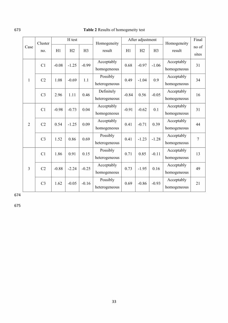
The H values of homogeneity test for all the three cases are given in Table 2. Initially, out of 354

the nine clusters (three clusters for each case), four clusters were acceptably homogeneous, 355

four clusters were possibly heterogeneous and one cluster was definitely heterogeneous. Hence, 356

adjustments were done to make the possibly and definitely heterogeneous clusters as 357

homogeneous, by either shifting discordant sites from one cluster to another or by removing 358

those sites if necessary. For case 1, stations Chubwa and Dilli were found to discordant with 359

all the clusters; hence they are removed during adjustment which lead to three acceptably 360

homogeneous clusters with the rest 81 stations. Similarly, station Chubwa was found to be 361

discordant for case 2; hence removed from the clusters and adjustments were done for 82 362

stations. However, in case 3, no stations were removed. The reason that the two stations did 363

not show any discordancy in case 3 is because the geographic locations of the stations were 364

considered during cluster analysis for case 3. The H values of homogeneity test after adjustment 365

and number of sites in each cluster are shown in Table 2. Final clusters formed after adjustment 366

are shown in Fig. 4a, 4b and 4c. 367

3.5 Comparison with similar studies done previously 368

17

Although this is the first and foremost study to divide the Brahmaputra valley region of India 369

into hydrologically homogeneous regions with the use of rainfall data record by the tea gardens 370

by applying fuzzy clustering technique and seven cluster validity indices (CVs), few previous 371

studies can be found on use of various clustering techniques for Indian subcontinent. Hence, 372

comparisons have been made with those closely related studies to validate the performance of 373

the present study. The homogeneous regions developed by Indian Meteorological Department 374

(IMD) displays five large provinces, which are although delineated based on rainfall 375

characteristics but are influenced by contiguity of area and administrative state boundaries. 376

Iyengar and Basak (1994) used principal component analysis (PCA) for regionalization of 377

Indian monsoon rainfall and recommended the PCA approach for further subdivision of the 378

region. Ten homogeneous sequential regions were formed in India from their analysis, in which 379

the stations of upper Brahmaputra valley regions were seemed to form similar kind of clusters 380

as found in the present study, although few stations remained un-clustered. Singh and Singh 381

(1996) have done regionalization of monthly as well as seasonal rainfall for sub-Himalayan 382

areas and Gangetic plains, by using principal component analysis (PCA). They used rainfall 383

data for a period of 114 years (1871-1984) from 90 well distributed stations which resulted into 384

four distinct homogeneous rainfall areas for both monthly and seasonal scales. Srinivasa and 385

Kumar (2007) utilized fuzzy cluster analysis (FCA) to classify 159 meteorological stations in 386

India and concluded that FCA method performs well than the Kohonen Artificial Neural 387

Networks (KANN) method in finding meteorologically homogeneous groups. They utilized 388

location parameters (latitude, longitude and elevation) along with other meteorological 389

parameters for clustering and the results exhibited 14 clusters over Indian region, the North-390

eastern region being in one cluster. Satyanarayana and Srinivas (2008) have done regional 391

frequency analysis using LSAVs that affects the precipitation in a region instead of observed 392

precipitation data and have used K-means clustering with adjustments and L-statistics for 393

18

regionalization. 17 homogeneous regions were formed after the analysis, two regions covering 394

the northeastern states. The upper Brahmaputra valley region came under the same 395

homogeneous cluster, hence producing similar results to those of the present study. 396

Satyanarayana and Srinivas (2011) have done regionalization of rainfall data, based on fuzzy 397

clustering method by utilizing GCM data, location parameters and seasonal precipitation data. 398

The stations of upper Brahmaputra valley regions were seemed to form similar kind of clusters 399

as found in the present study. Stations in middle Assam were found to form one cluster while 400

other stations on the upper Assam formed a different cluster. Saikranthi et al. (2013) used 401

correlation analysis for regionalization based on seasonal and annual rainfall data. They used 402

51 years (1951–2001) daily rainfall data collected for more than 1000 rain gauges across India 403

for the analysis, which produced 26 homogeneous rainfall zones. However, because of data 404

scarcity northeastern states were not included in the analysis. Bharath and Srinivas (2015) used 405

wavelet-based global FCM analysis, instead of PCA for determining homogeneous 406

hydrometeorological regions in India. The new approach proposed by them clustered the Indian 407

territory into 29 regions, northeastern region having 7 clusters. The clusters formed in the upper 408

Brahmaputra valley region were similar to the present study. Kulkarni (2017) has used 409

probability density function to divide the Indian subcontinent into homogeneous clusters, using 410

daily summer monsoon rainfall at 357 square grids of size 10000 sqkm. The study produced 411

five clusters, out of which one cluster covered adjoining regions and all other clusters were 412

scattered indicating irregular behaviour of daily rainfall pattern in India. The study was done 413

by using two time periods 1901–1975 and 1976–2010, and the resulting clusters were found to 414

be extremely different in the two time periods. The clusters formed in the northeastern region 415

is also different for the two periods which are not entirely in line with the present study. 416

However, they used gridded rainfall data instead of station data, thus the difference. Mannan 417

et al. (2018) have used climatic variables and self-organizing maps to regionalize India. 418

19

Artificial neural network is used along with four CVs for clustering and applied on gridded 419

rainfall dataset (0.25° × 0.25°) from IMD for 34 years (1980–2013) as well as climatic variables 420

such as air temperature, surface pressure, geo-potential height, specific humidity, etc. 10 421

homogeneous regions were formed when only rainfall data was used, whereas incorporation of 422

climatic variables divided the region into 15 regions. The region 2 in their study covered the 423

northeast India with rainfall of 7.2 mm/day. 424

4. Conclusion 425

In this paper, fuzzy clustering approach has been used to classify regions with homogeneous 426

rainfall in upper Brahmaputra Valley region of northeast India. Three different combinations 427

of feature vectors were employed in FCM algorithm to attain the best solutions to 428

regionalization. Seven different CVs were used to determine the optimal partition in the fuzzy 429

c-means (FCM) algorithm, out of which Extended Xie and beni index (VXB) and Kwon index 430

(VK) were opted for clustering of rainfall regions owing to their satisfactory performance. The 431

optimal value of cluster number for all three cases was identified as c=3, with corresponding 432

value of m=1.5. The clustered regions were then assessed for statistical homogeneity by 433

performing homogeneity tests using L-moment approach. Four clusters were found to be 434

acceptably homogeneous. Other possibly heterogeneous and definitely heterogeneous clusters 435

were made homogenous by adjusting the discordant sites. It was found from the results that the 436

clustering pattern was improved in case 3, where geographical location parameters (latitude, 437

longitude and elevation) were included along with local rainfall data of tea gardens. It indicates 438

that if regionalization needs to be done at a local scale such as an average sized watershed, 439

further sub-clustering of a clustered region may be required. Local rainfall data, along with 440

geographical location parameter details, can be used for the purpose since GCM data will not 441

be of much use in this aspect because of their coarse resolution. However, a good rainfall 442

dataset with large number of station points is required to be available within the region. 443

20

Acknowledgements 444

Authors acknowledge the teagarden authorities for making the data available. Our deepest 445

gratitude is extended to the editors and anonymous reviewers for their valuable comments and 446

suggestions. 447

Author’s Contribution 448

Conceptualization: Jayshree Hazarika, Arup Kumar Sarma; methodology: Jayshree Hazarika, 449

Arup Kumar Sarma; formal analysis and investigation: Jayshree Hazarika; writing - original 450

draft preparation: Jayshree Hazarika; writing - review and editing: Arup Kumar Sarma; 451

resources: Arup Kumar Sarma; supervision: Arup Kumar Sarma. 452

Funding 453

This research did not receive any specific grant from funding agencies in the public, 454

commercial, or not-for-profit sectors. 455

Availability of data and material 456

All relevant data are provided in both main manuscript and supplementary material. 457

Code availability 458

Not applicable 459

Declaration 460

Ethics approval All procedures performed in this study were in accordance with the ethical 461

standards of the institution or any comparable ethical standards. 462

Consent to participate We (authors) are agreed that Jayshree Hazarika planned, performed 463

the analysis, and wrote the paper, while Arup Kumar Sarma provided the resources and added 464

his expertise in the analysed results. 465

Consent for publication We give consent for our paper to be published in your Theoretical 466

and Applied Climatology journal. 467

21

Conflict of interest The authors have no conflicts of interest to declare that are relevant to the 468

content of this article. 469

References 470

Adelekan IO (1998) Spatio-temporal variations in thunderstorm rainfall over Nigeria. 471

International Journal of Climatology 18:1273–1284. https://doi.org/10.1002/(SICI)1097-472

0088(199809)18:11<1273::AID-JOC298>3.0.CO;2-4 473

Agarwal A, Maheswaran R, Sehgal V, Khosa R, Sivakumar B, Bernhofer C (2016) Hydrologic 474

regionalization using wavelet-based multiscale entropy method. Journal of Hydrology 538:22–475

32. https://doi.org/10.1016/j.jhydrol.2016.03.023 476

Asong ZE, Khaliq MN, Wheater HS (2015) Regionalization of precipitation characteristics in 477

the Canadian Prairie Provinces using large-scale atmospheric covariates and geophysical 478

attributes. Stochastic Environmental Research and Risk Assessment 29:875–892. 479

https://doi.org/10.1007/s00477-014-0918-z 480

Baltacı H, Göktürk OM, Kındap T, Ünal A, Karaca M (2015) Atmospheric circulation types in 481

Marmara Region (NW Turkey) and their influence on precipitation. International Journal of 482

Climatology 35:1810–1820. https://doi.org/10.1002/joc.4122 483

Baltacı H, Kındap T, Ünal A, Karaca M (2017) The influence of atmospheric circulation types 484

on regional patterns of precipitation in Marmara (NW Turkey). Theoretical and Applied 485

Climatology 127:563–572. https://doi.org/10.1007/s00704-015-1653-1 486

Bärring L (1987) Spatial patterns of daily rainfall in central Kenya: application of principal 487

component analysis and spatial correlation. Journal of Climatology 7(3):267–290. 488

https://doi.org/10.1002/joc.3370070306 489

Beable ME, McKercher AI (1982) Regional flood estimation in New Zealand. Water and Soil 490

Technical Publication 20, Ministry of works and development, Wellington. N.Z 491

22

Bedi HS, Bindra MMS (1980) Principal components of monsoon rainfall. Tellus 32(3):296–492

298. https://doi.org/10.3402/tellusa.v32i3.10584 493

Bezdek JC (1974a) Numerical taxonomy with fuzzy sets. Journal of Mathematical Biology 494

1(1):57–71. https://doi.org/10.1007/BF02339490 495

Bezdek JC (1974b) Cluster validity with fuzzy sets. Journal of Cybernetics 3(3):58–73. 496

https://doi.org/10.1080/01969727308546047 497

Bezdek JC (1981) Pattern recognition with fuzzy objective function algorithms. Plenum Press, 498

New York. https://doi.org/10.1007/978-1-4757-0450-1 499

Bezdek JC, Ehrlich R, Full W (1984) FCM: the fuzzy c-means clustering algorithm. Computers 500

& Geosciences 10:191–203. https://doi.org/10.1016/0098-3004(84)90020-7 501

Bharath R, Srinivas VV (2015) Delineation of homogeneous hydrometeorological regions 502

using wavelet-based global fuzzy cluster analysis. International Journal of Climatology 35: 503

4707–4727. https://doi.org/10.1002/joc.4318 504

Bonell M, Sumner G (1992) Atmospheric circulation and daily precipitation in Wales. 505

Theoretical and Applied Climatology 46:3–25. https://doi.org/10.1007/BF00866443 506

Burn DH (1997) Catchment similarity for regional flood frequency analysis using seasonality 507

measures. Journal of Hydrology 202:212–230. https://doi.org/10.1016/S0022-1694(97)00068-508

1 509

Chavoshi S, Azmin Sulaiman WN, Saghafian B, bin Sulaiman MN, Manaf LA (2013) 510

Regionalization by fuzzy expert system based approach optimized by genetic algorithm. 511

Journal of Hydrology 486:271–280. https://doi.org/10.1016/j.jhydrol.2013.01.033 512

Chen J, Zhao S, Wang H (2011) Risk Analysis of Flood Disaster Based on Fuzzy Clustering 513

Method. Energy Procedia 5:1915–1919. https://doi.org/10.1016/j.egypro.2011.03.329 514

23

Chew HH, Heiler M, David T (1987) Magnitude and frequency of floods in peninsular 515

malaysia (revised and updated) 1987, 1987th edn. Ministry of Agriculture and Fisheries, 516

Malayasia 517

Darand M, Daneshvar MRM (2014) Regionalization of precipitation regimes in Iran using 518

principal component analysis and hierarchical clustering analysis. Environmental Processes 519

1:517–532. https://doi.org/10.1007/s40710-014-0039-1 520

Dikbas F, Firat M, Koc AC, Gungor M (2012) Classification of precipitation series using fuzzy 521

cluster method. International Journal of Climatology 32:1596–1603. 522

https://doi.org/10.1002/joc.2350 523

Dinpashoh Y, Fakheri-Fard A, Moghaddam M, Jahanbakhsh S, Mirnia M (2004) Selection of 524

variables for the purpose of regionalization of Iran’s precipitation climate using multivariate 525

methods. Journal of Hydrology 297:109–123. https://doi.org/10.1016/j.jhydrol.2004.04.009 526

Dunn JC (1973) A fuzzy relative of the ISODATA process and its use in detecting compact, 527

well-separated clusters. Journal of Cybernetics 3(3):32–57. 528

https://doi.org/10.1080/01969727308546046 529

Efe B, Lupo AR, Deniz A (2019) The relationship between atmospheric blocking and 530

precipitation changes in Turkey between 1977 and 2016. Theoretical and Applied Climatology 531

138:1573–1590. https://doi.org/10.1007/s00704-019-02902-z 532

Farsadnia F, Kamrood MR, Nia AM, Modarres R, Bray MT, Han D, Sadatinejad J (2014) 533

Identification of homogeneous regions for regionalization of watersheds by two-level self-534

organizing feature maps. Journal of Hydrology 509:387–397. 535

https://doi.org/10.1016/j.jhydrol.2013.11.050 536

Fukuyama Y, Sugeno M (1989) A new method of choosing the number of clusters for the fuzzy 537

c-means method. Proceedings of Fifth Fuzzy Systems Symposium, pp. 247–250 (in Japanese). 538

24

Gadgil S, Yadumani, Joshi NV (1993) Coherent rainfall zones of the Indian region. 539

International Journal of Climatology 13(5):547–566. https://doi.org/10.1002/joc.3370130506 540

Goyal MK, Sharma A (2016) A fuzzy c-means approach regionalization for analysis of 541

meteorological drought homogeneous regions in western India. Natural Hazards 84(3):1831–542

1847. https://doi.org/10.1007/s11069-016-2520-9 543

Greenwood JA, Landwehr JM, Matalas NC, Wallis JR (1979) Probability weighted moments: 544

definition and relation to parameters of several distributions expressible in inverse form. Water 545

Resources Research 15(5):1049–1054. https://doi.org/10.1029/WR015i005p01049 546

Guttman NB (1993) The Use of L-Moments in the Determination of Regional Precipitation 547

Climates. Journal of Climate 6:2309–2325. https://doi.org/10.1175/1520-548

0442(1993)006<2309:TUOLMI>2.0.CO;2 549

Halkidi M, Batistakis Y, Vazirgiannis M (2001) On clustering validation techniques. Journal 550

of Intelligent Information Systems 17:107–145. https://doi.org/10.1023/A:1012801612483 551

Hall MJ, Minns AW (1999) The classification of hydrologically homogeneous regions. 552

Hydrological Sciences Journal 44(5):693–704. https://doi.org/10.1080/02626669909492268 553

Hosking JRM (1990) L-moments: Analysis and estimation of distributions using linear 554

combinations of order statistics. Journal of the Royal Statistical Society: Series B 555

(Methodological) banner 52(1):105–124. https://doi.org/10.1111/j.2517-6161.1990.tb01775.x 556

Hosking JRM, Wallis JR (1993) Some Statistics useful in regional frequency analysis. Water 557

Resources Research 29(2):271–281. https://doi.org/10.1029/92WR01980 558

Hosking JRM, Wallis JR (1995) Correction to “Some statistics useful in regional frequency 559

analysis”. Water Resources Research 31(1):251. https://doi.org/10.1029/94WR02510 560

Hosking JRM, Wallis JR (1997) Regional frequency analysis: an approach based on L-561

moments. Cambridge University Press, Cambridge. 562

https://doi.org/10.1017/CBO9780511529443 563

25

Irwin S, Srivastav RK, Simonovic SP, Burn DH (2017) Delineation of precipitation regions 564

using location and atmospheric variables in two Canadian climate regions: the role of attribute 565

selection. Hydrological Sciences Journal 62:191–204. 566

https://doi.org/10.1080/02626667.2016.1183776 567

Iyengar RN, Basak P (1994) Regionalization of Indian monsoon rainfall and long-term 568

variability signals. International Journal of Climatology 14:1095–1114. 569

https://doi.org/10.1002/joc.3370141003 570

Karaca M, Deniz A, Tayanc M (2000) Cyclone Track Variability Over Turkey in Association 571

with Regional Climate. International Journal of Climatology 20:1225–1236. 572

https://doi.org/10.1002/1097-0088(200008)20:10%3C1225::AID-JOC535%3E3.0.CO;2-1 573

Kulkarni A (2017) Homogeneous clusters over India using probability density function of daily 574

rainfall. Theoretical and Applied Climatology 129:633–643. https://doi.org/10.1007/s00704-575

016-1808-8 576

Kulkarni A, Kripalani RH, Singh SV (1992) Classification of summer monsoon rainfall 577

patterns over India. International Journal of Climatology 12(3):269–280. 578

https://doi.org/10.1002/joc.3370120304 579

Kwon SH (1998) Cluster Validity Index for Fuzzy Clustering. Electronics Letters 580

34(22):2176–2177. https://doi.org/10.1049/el:19981523 581

Machiwal D, Kumar S, Meena HM, Santra P, Singh RK, Singh DV (2019) Clustering of 582

rainfall stations and distinguishing influential factors using PCA and HCA techniques over the 583

western dry region of India. Meteorological Applications 26:300–311. 584

https://doi.org/10.1002/met.1763 585

Mannan A, Chaudhary S, Dhanya CT, Swamy AK (2018) Regionalization of rainfall 586

characteristics in India incorporating climatic variables and using self-organizing maps. ISH 587

26

Journal of Hydraulic Engineering 24(2):147–156. 588

https://doi.org/10.1080/09715010.2017.1400409 589

Mok PY, Huang HQ, Kwok YL, Au JS (2012) A robust adaptive clustering analysis method 590

for automatic identification of clusters. Pattern Recognition 45:3017–3033. 591

https://doi.org/10.1016/j.patcog.2012.02.003 592

NERC (1975) Flood Studies Report, five volumes. Natural Environmental Research Council 593

(NERC), Department of the Environment, London 594

Owen SM, MacKenzie AR, Bunce RGH, Stewart HE, Donovan RG, Stark G, Hewitt CN 595

(2006) Urban land classification and its uncertainties using principal component and cluster 596

analyses: A case study for the UK West Midlands. Landscape and Urban Planning 78:311–597

321. https://doi.org/10.1016/j.landurbplan.2005.11.002 598

Pal NR, Bezdek JC (1995) On cluster validity for the fuzzy c-means model. IEEE Transactions 599

on Fuzzy Systems 3(3):370–379. https://doi.org/10.1109/91.413225 600

Pelczer I, Ramos J, Domínguez R, González F (2007) Establishment of regional homogeneous 601

zones in a watershed using clustering algorithms. In: 32 Congress of IAHR Harmonizing the 602

Demands of Art and Nature in Hydraulics, IAHR, Venice, Italy, File. 603

http://citeseerx.ist.psu.edu/viewdoc/summary?doi=10.1.1.107.3470 604

Plain MB, Minasny B, McBratney AB, Vervoort RW (2008) Spatially explicit seasonal 605

forecasting using fuzzy spatiotemporal clustering of long-term daily rainfall and temperature 606

data. Hydrology and Earth System Sciences Discussions 5:1159–1189. 607

https://doi.org/10.5194/hessd-5-1159-2008 608

Rao AR, Srinivas VV (2006a) Regionalization of watersheds by hybrid-cluster analysis. 609

Journal of Hydrology 318:37–56. https://doi.org/10.1016/j.jhydrol.2005.06.003 610

Rao AR, Srinivas VV (2006b) Regionalization of watersheds by fuzzy cluster analysis. Journal 611

of Hydrology 318:57–79. https://doi.org/10.1016/j.jhydrol.2005.06.004 612

27

Roubens M (1982) Fuzzy clustering algorithms and their cluster validity. European Journal of 613

Operational Research 10:294–301. https://doi.org/10.1016/0377-2217(82)90228-4 614

Sadri S, Burn DH (2011) A Fuzzy C-Means approach for regionalization using a bivariate 615

homogeneity and discordancy approach. Journal of Hydrology 401:231–239. 616

https://doi.org/10.1016/j.jhydrol.2011.02.027 617

Saikranthi K, Rao TN, Rajeevan M, Bhaskara Rao SV (2013) Identification and Validation of 618

Homogeneous Rainfall Zones in India Using Correlation Analysis. Journal of 619

Hydrometeorology 14:304–317. https://doi.org/10.1175/JHM-D-12-071.1 620

Satyanarayana P, Srinivas VV (2008) Regional frequency analysis of precipitation using large-621

scale atmospheric variables. Journal of Geophysical Research 113:1–16. 622

https://doi.org/10.1029/2008JD010412 623

Satyanarayana P, Srinivas VV (2011) Regionalization of precipitation in data sparse areas 624

using large scale atmospheric variables – A fuzzy clustering approach. Journal of Hydrology 625

405:462–473. https://doi.org/10.1016/j.jhydrol.2011.05.044 626

Singh KK, Singh SV (1996) Space-time variation and regionalization of seasonal and monthly 627

summer monsoon rainfall of the sub-Himalayan region and Gangetic plains of India. Climate 628

Research 6:251–262. https://doi.org/10.3354/cr006251 629

Srinivas VV, Tripathi S, Rao AR, Govindaraju RS (2008) Regional flood frequency analysis 630

by combining self-organizing feature map and fuzzy clustering. Journal of Hydrology 631

348:148–166. https://doi.org/10.1016/j.jhydrol.2007.09.046 632

Srinivasa RK, Nagesh KD (2007) Classification of Indian meteorological stations using cluster 633

and fuzzy cluster analysis, and Kohonen artificial neural networks. Nordic Hydrology 634

38(3):303–314. https://doi.org/10.2166/nh.2007.013 635

28

Sumner G, Bonell M (1988) Variation in the spatial organisation of daily rainfall during the 636

north Queensland wet seasons, 1979–82. Theoretical and Applied Climatology 39:59–72. 637

https://doi.org/10.1007/BF00866390 638

Thomas DM, Benson M a (1970) Generalization of streamflow characteristics from drainage-639

basin characteristics. https://doi.org/10.3133/wsp1975 640

Unal Y, Kindap T, Karaca M (2003) Redefining the climate zones of Turkey using cluster 641

analysis. International Journal of Climatology 23:1045–1055. https://doi.org/10.1002/joc.910 642

Unal YS, Deniz A, Toros H, Incecik S (2012) Temporal and spatial patterns of precipitation 643

variability for annual, wet, and dry seasons in Turkey. International Journal of Climatology 644

32(3):392–405. https://doi.org/10.1002/joc.2274 645

Venkatesh B, Jose MK (2007) Identification of homogeneous rainfall regimes in parts of 646

Western Ghats region of Karnataka. Journal of Earth System Science 116(4):321–329. 647

https://doi.org/10.1007/s12040-007-0029-z 648

Viglione A, Laio F, Claps P (2007) A comparison of homogeneity tests for regional frequency 649

analysis. Water Resources Research 43(W03428):1–10. 650

https://doi.org/10.1029/2006WR005095 651

Wang Z, Zeng Z, Lai C, Lin W, Wu X, Chen X (2017) A regional frequency analysis of 652

precipitation extremes in Mainland China with fuzzy c-means and L-moments approaches. 653

International Journal of Climatology 37: 429–444. https://doi.org/10.1002/joc.5013 654

Wotling G, Bouvier C, Danloux J, Fritsch J-M (2000) Regionalization of extreme precipitation 655

distribution using the principal components of the topographical environment. Journal of 656

Hydrology 233:86–101. https://doi.org/10.1016/S0022-1694(00)00232-8 657

Xie XL, Beni G (1991) A validity measure for fuzzy clustering. IEEE Transactions on Pattern 658

Analysis and Machine Intelligence 13(8):841–847. https://doi.org/10.1109/34.85677 659

660

29

LIST OF TABLES 661

Table 1 Location details of raingauge stations located in various tea gardens of the upper 662

Brahmaputra valley region with mean annual and seasonal precipitation 663

Table 2 Results of homogeneity test 664

665

30

Table 1 Location details of raingauge stations located in various tea gardens of the upper 666

Brahmaputra valley region with mean annual and seasonal precipitation 667

Sl. No. Name of the

station

Longitude

(0E)

Latitude

(0N)

Seasonal rainfall in mm Total annual

rainfall in mm

Elevation

in m DJF MAM JJA SON

1 Abhoijan 93.8986111 26.4225 70 610 1127 510 2317 121

2 Achabam 95.2644444 27.24 82 579 1249 401 2312 123

3 Amsoi 92.4102778 26.1433333 31 326 843 346 1546 67

4 Anand 94.2300797 27.4619764 101 525 1880 719 3225 112

5 Arin 93.9752778 26.4877778 49 478 831 321 1679 100

6 Arun 92.4402778 26.6669444 32 451 823 257 1563 80

7 Athabari 94.0347222 26.4138889 9 301 525 162 996 104

8 Azizbagh 95.1302778 27.2063889 111 698 1354 479 2642 113

9 Bahani 94.2025 26.7555556 79 552 905 449 1985 93

10 Basmatia 95.0671167 27.3605556 81 637 1126 409 2253 113

11 Bateli 92.2537422 26.7759589 35 430 907 340 1712 112

12 Bhelaguri 94.3846566 26.7048311 57 489 830 279 1654 116

13 Bokajan 93.7751667 26.022 22 260 548 254 1084 136

14 Bokakhat 93.6438889 26.6377778 58 553 975 382 1968 87

15 Borahi 94.9902778 27.0433333 59 684 1291 454 2488 104

16 Borchapori 93.6899 26.6381972 75 550 1143 406 2174 92

17 Borhat 95.2888889 27.1388889 29 238 406 187 859 122

18 Borjan 94.0577778 26.5619444 39 393 745 271 1448 104

19 Borpathar 93.8488889 26.2722222 44 404 708 274 1430 127

20 Chubwa 95.1730556 27.4661111 99 835 1447 601 2981 118

21 Cinnatolliah 94.0857124 27.342037 110 653 1709 589 3061 123

22 Dalowjan 93.9747222 26.4338889 54 425 729 347 1555 105

23 Deamoolie 95.5388889 27.5905556 91 670 1275 442 2478 134

24 Dejoo 94.0031433 27.2807217 106 661 1690 544 3002 123

25 Dekorai 92.9636778 26.81 56 608 1238 445 2347 83

26 Deohall 95.2890372 27.4223095 103 710 1152 379 2344 125

27 Dhekiajuli 92.4615703 26.6904332 57 572 1090 391 2110 77

28 Dholaguri 93.84161 26.5128231 49 479 822 272 1622 99

31

29 Digulturrung 95.4119444 27.6104528 58 631 905 309 1903 126

30 Dilli 95.3672222 27.1638889 118 732 1507 519 2877 132

31 Diphloo 93.5685556 26.6394444 31 578 910 303 1822 84

32 Dooria 93.9191667 26.6316667 46 460 927 242 1675 97

33 Duklingia 94.2852151 26.6861544 74 685 1329 428 2515 112

34 Durrung 92.7297222 26.7227778 50 445 768 271 1534 76

35 Furkating 94.0137903 26.4617283 55 395 768 318 1535 106

36 Halem 93.4523611 26.8696667 44 449 1022 341 1856 90

37 Halmira 93.9466667 26.5241667 47 468 832 340 1688 101

38 Harchurah 92.7537139 26.7775488 61 561 1226 435 2282 94

39 Hatigarh 94.0433333 26.3888889 44 452 785 309 1590 102

40 Hatikhuli 93.370899 26.5848439 51 540 906 373 1870 87

41 Kakojan 94.3886111 26.735 46 440 786 247 1518 107

42 Kellyden 92.948746 26.483845 41 440 927 292 1700 86

43 Keyhung 95.3279024 27.4345426 101 658 1238 461 2457 127

44 Khowang 94.8938766 27.2431657 80 627 1052 337 2096 103

45 Koomsong 95.6537533 27.6188283 109 925 1182 476 2693 144

46 Kopati 92.25073 26.59 45 504 839 297 1685 75

47 Lakwa 94.8722222 27.0244444 93 607 1286 429 2416 100

48 Lamabari 92.277784 26.842633 35 504 1218 408 2166 134

49 Ledo 95.7683333 27.3020278 77 392 577 288 1333 153

50 Lengeree 93.7166667 25.9211111 41 299 711 302 1354 154

51 Lepetkata 94.8635316 27.3783221 222 649 1113 417 2402 104

52 Madhuting 95.3667005 27.3581907 27 262 451 157 897 129

53 Mahalakshmi 93.0608333 26.8555556 28 432 733 280 1473 88

54 Maijan 94.9783246 27.5079422 118 623 1359 529 2629 111

55 Mancotta 94.9175806 27.4385028 130 865 1764 653 3412 108

56 Mazbat 92.2515106 26.7810162 37 559 1185 379 2160 113

57 Moran 94.8846352 27.1563477 72 609 1060 405 2146 103

58 Murphuloni 93.9247879 26.457985 36 495 868 295 1694 106

59 Nahorjan 93.6065063 26.6075556 62 553 895 302 1812 98

60 Namburnodi 93.83188 26.29877 50 399 731 326 1506 134

61 Namdang 95.7220833 27.2655556 111 730 1555 534 2930 427

32

62 Namrup 95.3286111 27.1947222 50 429 731 256 1465 125

63 Nitinnagar 94.052032 26.345432 35 294 561 223 1113 107

64 Nonoi 92.9216667 26.4041667 35 487 1090 383 1994 79

65 Ouphulia 95.0147222 27.2177778 92 704 1350 493 2639 109

66 Paneery 91.8962681 26.7463385 64 680 1057 453 2254 122

67 Panitola 95.2573121 27.4941394 95 470 1087 463 2114 124

68 Pavoijan 93.9055538 26.2978396 44 371 654 275 1344 116

69 Powai 95.6482333 27.3478431 77 613 1262 377 2329 158

70 Rungamatty 93.8986111 26.6702778 53 543 894 335 1825 90

71 Rupai 95.4952778 27.6123056 111 726 1313 458 2608 132

72 Rupajuli 92.7217448 26.7260395 53 584 1225 440 2301 78

73 Sagmootea 93.004862 26.544426 49 480 1013 309 1851 92

74 Santi 95.4125 27.3038889 102 965 1368 447 2882 127

75 Sepoi 92.4102034 26.7837818 17 704 1077 327 2125 110

76 Sepon 94.845947 27.1150673 77 584 1141 394 2195 103

77 Sockeiting 94.087428 26.546912 57 422 900 314 1693 98

78 Sonabheel 92.7849483 26.7369584 48 465 1045 364 1921 76

79 Sundarpur 95.1924133 27.1453118 53 725 1612 656 3046 113

80 Teloijan 94.9437618 27.2513485 55 355 798 329 1537 103

81 Tezpore &

gogra

92.7395976 26.7232366 61 570 1030 359 2020 79

82 Thanai 95.0936111 27.5357694 73 576 1071 396 2116 116

83 Uday jyoti 93.9638889 26.5 19 383 678 264 1344 99

Note: DJF = December, January, February 668

MAM = March, April, May 669

JJA = June, July, August 670

SON = September, October, November 671

672

33

Table 2 Results of homogeneity test 673

Case Cluster

no.

H test Homogeneity

result

After adjustment Homogeneity

result

Final

no of

sites H1 H2 H3 H1 H2 H3

1

C1 -0.08 -1.25 -0.99 Acceptably

homogeneous 0.68 -0.97 -1.06

Acceptably

homogeneous 31

C2 1.08 -0.69 1.1 Possibly

heterogeneous 0.49 -1.04 0.9

Acceptably

homogeneous 34

C3 2.96 1.11 0.46 Definitely

heterogeneous -0.84 0.56 -0.05

Acceptably

homogeneous 16

2

C1 -0.98 -0.73 0.04 Acceptably

homogeneous -0.91 -0.62 0.1

Acceptably

homogeneous 31

C2 0.54 -1.25 0.09 Acceptably

homogeneous 0.41 -0.71 0.39

Acceptably

homogeneous 44

C3 1.52 0.86 0.69 Possibly

heterogeneous 0.41 -1.23 -1.28

Acceptably

homogeneous 7

3

C1 1.86 0.91 0.15 Possibly

heterogeneous 0.71 0.85 -0.11

Acceptably

homogeneous 13

C2 -0.88 -2.24 -0.25 Acceptably

homogeneous 0.73 -1.95 0.16

Acceptably

homogeneous 49

C3 1.62 -0.05 -0.16 Possibly

heterogeneous 0.69 -0.86 -0.93

Acceptably

homogeneous 21

674

675

34

LIST OF FIGURES 676

Fig. 1 Methodology used to identify homogeneous rainfall regions 677

Fig. 2 Raingauge stations located in various tea gardens of the upper Brahmaputra valley region 678

Fig. 3 Variation in the optimum value of objective function of FCM algorithm with variation of 679

fuzzifier m and cluster number c, for (a) Case 1: with total monthly rainfall as attributes; (b) Case 2: 680

with standard deviation of total monthly rainfall as attributes; and (c) Case 3: with latitude, longitude, 681

elevation, total annual rainfall and standard deviation of total annual rainfall as attributes 682

Fig. 4 Clusters formed by the FCM algorithm after adjustment for (a) Case 1: with total monthly 683

rainfall as attributes; (b) Case 2: with standard deviation of total monthly rainfall as attributes; and (c) 684

Case 3: with latitude, longitude, elevation, total annual rainfall and standard deviation of total annual 685

rainfall as attributes 686

687

35

688

Fig. 1 Methodology used to identify homogeneous rainfall regions 689

690

Form fuzzy clusters applying FCM algorithm

Identify optimum cluster number by using

cluster validity indices

Test whether

the clusters are

homogeneous

Adjust the

heterogeneous

clusters

Homogeneous rainfall

regions

No

Yes

36

691

Fig. 2 Raingauge stations located in various tea gardens of the upper Brahmaputra valley region 692

693

37

(a) Case 1

(b) Case 2

0

100

200

300

400

500

600

700

1.1 1.2 1.3 1.4 1.5 1.6 1.7 1.8 1.9 2 2.1 2.2 2.3 2.4 2.5 2.6 2.7 2.8 2.9 3

Ob

ject

ive

fu

nct

ion

Fuzzifier

no. of cluster=2

no. of cluster=3

no. of cluster=4

no. of cluster=5

no. of cluster=6

no. of cluster=7

no. of cluster=8

no. of cluster=9

no. of cluster=10

0

100

200

300

400

500

600

700

1.1 1.2 1.3 1.4 1.5 1.6 1.7 1.8 1.9 2 2.1 2.2 2.3 2.4 2.5 2.6 2.7 2.8 2.9 3

Ob

ject

ive

fu

nct

ion

Fuzzifier

no. of cluster=2

no. of cluster=3

no. of cluster=4

no. of cluster=5

no. of cluster=6

no. of cluster=7

no. of cluster=8

no. of cluster=9

no. of cluster=10

38

(c) Case 3

Fig. 3 Variation in the optimum value of objective function of FCM algorithm with variation of 694

fuzzifier m and cluster number c, for (a) Case 1: with total monthly rainfall as attributes; (b) Case 2: 695

with standard deviation of total monthly rainfall as attributes; and (c) Case 3: with latitude, longitude, 696

elevation, total annual rainfall and standard deviation of total annual rainfall as attributes 697

698

0

100

200

300

400

500

600

700

1.1 1.2 1.3 1.4 1.5 1.6 1.7 1.8 1.9 2 2.1 2.2 2.3 2.4 2.5 2.6 2.7 2.8 2.9 3

Ob

ject

ive

fu

nct

ion

Fuzzifier

no. of cluster=2

no. of cluster=3

no. of cluster=4

no. of cluster=5

no. of cluster=6

no. of cluster=7

no. of cluster=8

no. of cluster=9

no. of cluster=10

39

(a) Case 1

40

(b) Case 2

(c) Case 3

699

Fig. 4 Clusters formed by the FCM algorithm after adjustment for (a) Case 1: with total monthly 700

rainfall as attributes; (b) Case 2: with standard deviation of total monthly rainfall as attributes; and (c) 701

Case 3: with latitude, longitude, elevation, total annual rainfall and standard deviation of total annual 702

rainfall as attributes 703

704

Figures

Figure 1

Methodology used to identify homogeneous rainfall regions

Figure 2

Raingauge stations located in various tea gardens of the upper Brahmaputra valley region. Note: Thedesignations employed and the presentation of the material on this map do not imply the expression ofany opinion whatsoever on the part of Research Square concerning the legal status of any country,territory, city or area or of its authorities, or concerning the delimitation of its frontiers or boundaries. Thismap has been provided by the authors.

Figure 3

Variation in the optimum value of objective function of FCM algorithm with variation of fuzzi�er m andcluster number c, for (a) Case 1: with total monthly rainfall as attributes; (b) Case 2: with standarddeviation of total monthly rainfall as attributes; and (c) Case 3: with latitude, longitude, elevation, totalannual rainfall and standard deviation of total annual rainfall as attributes

Figure 4

Clusters formed by the FCM algorithm after adjustment for (a) Case 1: with total monthly rainfall asattributes; (b) Case 2: with standard deviation of total monthly rainfall as attributes; and (c) Case 3: withlatitude, longitude, elevation, total annual rainfall and standard deviation of total annual rainfall asattributes. Note: The designations employed and the presentation of the material on this map do notimply the expression of any opinion whatsoever on the part of Research Square concerning the legal

status of any country, territory, city or area or of its authorities, or concerning the delimitation of itsfrontiers or boundaries. This map has been provided by the authors.

Supplementary Files

This is a list of supplementary �les associated with this preprint. Click to download.

SupplementaryMaterial.docx