Important Variables of a RapidEye Time Series for ... · Thorsten Dahms et al., Important Variables of a RapidEye Time Series 287 spectral indices or band selection can be use-ful

PFG 2016 / 5 – 6, 285 – 299 ArticleStuttgart, December 2016

© 2016 E. Schweizerbart'sche Verlagsbuchhandlung, Stuttgart, Germany www.schweizerbart.deDOI: 10.1127/pfg/2016/0303 1432-8364/16/0303 $ 3.75

Important Variables of a RapidEye Time Series for Modelling Biophysical Parameters of Winter Wheat

ThorsTen dahms, sylvia seissiger, Würzburg, eriK borg, hermann vaJen, bernd FichTelmann, Neustrelitz & chrisToPher conrad, Würzburg

Keywords: biophysical parameter, RapidEye, vegetation indices, winter wheat, phenology, conditional inference forest

Summary: With the increasing availability of high resolution data, remote sensing is gaining impor-tance for agricultural management. Sensor constel-lations such as RapidEye or Sentinel-2 have a strong potential for precision agriculture because they pro-vide spectral information throughout the cropping season and at the subfield level. To explore this po-tential, methods are required that accurately trans-fer the spectral information into biophysical param-eters which in turn permit quantitative assessments of plant growth on the field. Boundary condition for a successful monitoring, e.g., a repeated derivation of the biophysical parameters is to cope with the challenge of enormous data amounts, i.e. to select the input data that is most relevant.

In this study, biophysical parameters of winter wheat, namely the fraction of absorbed photosyn-thetic active radiation (FPAR), the leaf area index (LAI) and the chlorophyll content (expressed by SPAD), were modelled with RapidEye data in Mecklenburg-West Pomerania, Germany, using Random Forest based on conditional inference trees. Focus was set at the selection of the most im-portant information out of spectral bands and indi-ces for parameter prediction on winter wheat. In-situ and remote sensing observations were grouped into phenological phases in order to examine the importance of single spectral bands or indices for modelling biophysical reality in the several grow-ing stages of winter wheat. The coefficient of deter-mination for FPAR (LAI; SPAD) ranged between 0.19 and 0.83 (0.33 and 0.66; 0.21 and 0.45). Model accuracy was linked with the phenological phase. The results showed that for each biophysical pa-rameter, different spectral variables become im-portant for modelling and the number of important variables depends on the phenological time span. The prediction of biophysical parameters for short phenological groups often depends only on one to

three variables. The results also showed that in the phenological phase of fruit development, the model accuracy is the lowest and the determination of the importance is comparatively vague.

Zusammenfassung: Wichtige Variablen aus Rapid-Eye-Zeitreihen für die Modellierung biophysikali-scher Parameter von Winterweizen. Hochaufgelös-tes Monitoring agrarwirtschaftlicher Flächen ge-winnt immer mehr an Bedeutung. Aus fernerkund-licher Sicht beruht dieses Monitoring auf der robus-ten Ableitung verschiedener biophysikalischer Pa-rameter aus räumlich und zeitlich hoch aufgelösten Fernerkundungsdaten, z.B. RapidEye oder Senti-nel-2. Ziel aktueller Forschung ist es, die biophysi-kalischen Parameter FPAR (Fraction of Absorbed Photosynthetic Active Radiation), LAI (Leaf Area Index) und den Chlorophyllgehalt aus fernerkund-lichen Daten zu ermitteln. Hierbei reizen die gro-ßen Datenmengen häufig die Berechnungskapazi-täten aus. Somit wird eine umsichtige Reduzierung der zu verarbeitenden Datenmenge die Anwend-barkeit dieser Methode verbessern.

In der vorliegenden Studie wurden conditional inference Random Forests eingesetzt, um zum ei-nen die biophysikalischen Parameter unter Ver-wendung von RapidEye Szenen zu modellieren, und zum anderen die Bedeutung der einzelnen Ein-gangsparameter (Spektrale Bänder des RapidEye und Vegetationsindizes) zu quantifizieren. Die di-rekt auf dem Feld und die fernerkundlich erhobe-nen Beobachtungen des Winterweizens wurden in unterschiedliche Entwicklungsstadien (phänologi-sche Gruppen) eingeteilt. Bei der Modellierung des FPAR (LAI; SPAD) wurden hierbei Bestimmt-heitsmaße zwischen 0.19 und 0.83 (0.33 und 0.66; 0.21 und 0.45) erreicht. Dies zeigt, dass die Genau-igkeit der Modellierung der jeweiligen biophysika-lischen Parameter stark von der entsprechenden

286 Photogrammetrie • Fernerkundung • Geoinformation 5 – 6/2016

1 Introduction

Recently launched and upcoming satellite missions like the Sentinel systems will high-ly increase the amount of spatiotemporal data provided by remote sensing (bonteMPs et al. 2015). This kind of high resolution data offers great opportunities among others in agricul-ture (FranKe & Menz 2007). Remote sensing based information of high spatial and tempo-ral resolution can for instance be beneficial for agricultural applications like precision farm-ing and crop yield estimation (Haboudane et al. 2004, aHMadian et al. 2016). These appli-cations demand accurate and up to date infor-mation on the vegetation (Jin et al. 2013), e.g. on the phenological state and on vegetation growth such as biomass production, e.g. ex-pressed by absorbed photosynthetically active radiation (FPAR), the leaf area index (LAI), or chlorophyll content. One example is the study of eitel et al. (2007), where the nitrogen sta-tus of winter wheat was predicted to support farmers with the information whether to ap-ply supplemental fertilizer during the growing period of the crop. However, such applications useful for precision agriculture are still rare.

In order to observe and analyse vegeta-tion using biophysical parameters, several re-mote sensing approaches were proposed in the past (Hall et al. 1995, Mutanga & sKidMore 2004, le Maire et al. 2011). One option is em-pirical modelling, i.e. the identification of an optimal statistical relation between spectral measurements, e.g. vegetation indices, and in situ observations. The suitability of empirical approaches varies among the biophysical pa-rameters because they vary in their complex-ity. Linear statistical approaches may be suf-ficient for the derivation of FPAR at least for

phänologischen Gruppe abhängt. Darüber hinaus zeigen die Ergebnisse, dass die Bedeutung der un-terschiedlichen Eingangsparameter für die unter-schiedlichen biophysikalischen Parameter und un-terschiedlichen Entwicklungsstadien stark unter-schiedlich ist. Häufig sind es nur bis zu drei spek-

trale Variable, die einen Parameter in den kurzen Entwicklungsphasen beschreiben. Die Ergebnisse zeigen auch, dass das Modellieren biophysikali-scher Parameter im phänologischen Stadium der Fruchtreife am ungenauesten ist.

some crops (Myneni & WilliaMs 1994, leX et al. 2013). However, e.g. for the derivation of LAI, there are strong indications that one vegetation index or spectral band cannot ex-plain the biophysical reality of the vegetation cover over the entire growing season (Viña et al. 2011, leX et al. 2013), because the physi-cal appearance of the crop and, moreover, can-opy parameters like cover fraction and plant height vary with the phenological stages of crops. Thus and not exclusively for crops, dif-ferent univariate and multivariate, linear and non-linear statistical methods have been ap-plied for monitoring biophysical parameters of vegetation with high-resolution data. Ma-chine learning algorithms such as the Ran-dom Forest algorithm (breiMan 2001) are typically able to cope with a strong non-lin-earity of the functional dependence between some biophysical parameters and the reflected spectra (becKscHaeFer et al. 2014). Differen-tiation among different phenological stages could also improve empirical estimations of biophysical parameters of vegetation, at least for some growing stages of vegetation, as e.g. shown by tillacK et al. (2014) or leX et al. (2015). Nevertheless, little attention has been put on the derivation of biophysical parame-ters using high resolution remote sensing data in combination with machine learning algo-rithms for crop monitoring at different stages of the vegetation period.

One challenge to increase the practical use of remote sensing based information products for precision agriculture is the enormous ex-penditure (e.g. data amount, storage space, processing time), which is necessary for the derivation of the relevant biophysical param-eters. To minimize this aspect the reduction of the spectral resolution, e.g. by composing

Thorsten Dahms et al., Important Variables of a RapidEye Time Series 287

spectral indices or band selection can be use-ful and information is required, which indi-ces and spectral bands have the most effect on modelling biophysical parameters at which growing stage. Machine learning methods provide an assessment of the so-called vari-able importance, which returns the relevance and suitability of certain spectral bands and indices for accurate modelling of biophysical parameters. becKscHaeFer et al. (2014) dem-onstrated the usability of the variable impor-tance when linking remote sensing observa-tions with biophysical parameters for subtrop-ical upland ecosystems.

Different remote sensing applications deal with the extraction of variable importance from Random Forests (Mutanga et al. 2012, becKscHaeFer et al. 2014). However, strobl et al. (2007) pointed out that an analysis of caus-al effects using the classical Random Forest approach can be biased in case of having cor-related regressors. Against this background, strobl et al. (2008) introduced the condition-al variable importance method to determine the variable importance for correlated regres-sors. In cause-effect analyses based on Ran-dom Forest, in which remote sensing data is utilized, this conditional variable importance method is critical, because spectral bands or e.g. vegetation indices are commonly highly correlated.

The aims of this study are (i) to predict bi-ophysical parameters, namely FPAR, LAI, chlorophyll content of winter wheat during the different growing stages using RapidEye time series and in-situ data, (ii) to identify the most important spectral bands or indices for modelling these biophysical parameters and (iii) to investigate how the indicator impor-tance of these variables changes in the pheno-logical cycle.

2 Study Area

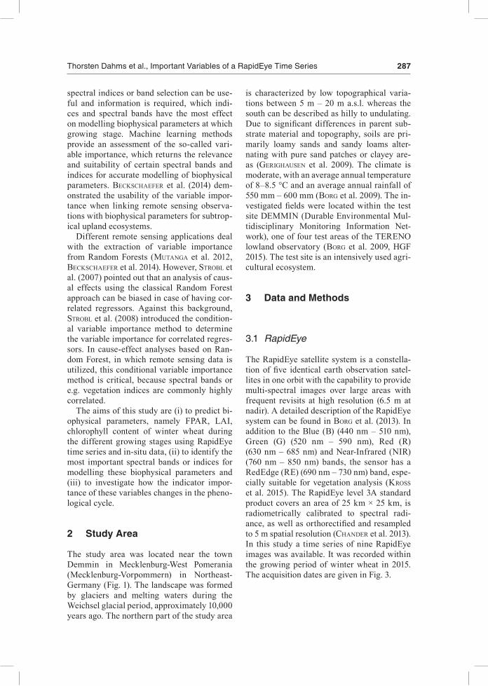
The study area was located near the town Demmin in Mecklenburg-West Pomerania (Mecklenburg-Vorpommern) in Northeast-Germany (Fig. 1). The landscape was formed by glaciers and melting waters during the Weichsel glacial period, approximately 10,000 years ago. The northern part of the study area

is characterized by low topographical varia-tions between 5 m – 20 m a.s.l. whereas the south can be described as hilly to undulating. Due to significant differences in parent sub-strate material and topography, soils are pri-marily loamy sands and sandy loams alter-nating with pure sand patches or clayey are-as (gerigHausen et al. 2009). The climate is moderate, with an average annual temperature of 8–8.5 °C and an average annual rainfall of 550 mm – 600 mm (borg et al. 2009). The in-vestigated fields were located within the test site DEMMIN (Durable Environmental Mul-tidisciplinary Monitoring Information Net-work), one of four test areas of the TERENO lowland observatory (borg et al. 2009, HGF 2015). The test site is an intensively used agri-cultural ecosystem.

3 Data and Methods

3.1 RapidEye

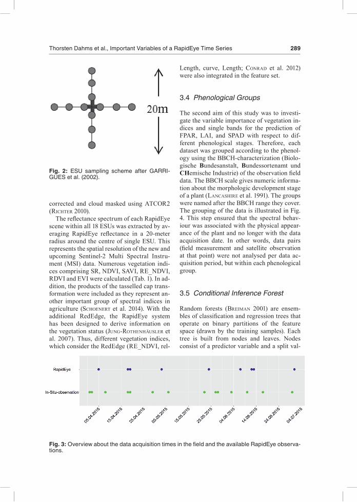
The RapidEye satellite system is a constella-tion of five identical earth observation satel-lites in one orbit with the capability to provide multi-spectral images over large areas with frequent revisits at high resolution (6.5 m at nadir). A detailed description of the RapidEye system can be found in borg et al. (2013). In addition to the Blue (B) (440 nm – 510 nm), Green (G) (520 nm – 590 nm), Red (R) (630 nm – 685 nm) and Near-Infrared (NIR) (760 nm – 850 nm) bands, the sensor has a RedEdge (RE) (690 nm – 730 nm) band, espe-cially suitable for vegetation analysis (Kross et al. 2015). The RapidEye level 3A standard product covers an area of 25 km × 25 km, is radiometrically calibrated to spectral radi-ance, as well as orthorectified and resampled to 5 m spatial resolution (cHander et al. 2013). In this study a time series of nine RapidEye images was available. It was recorded within the growing period of winter wheat in 2015. The acquisition dates are given in Fig. 3.


3.2 In-situ Observations

In diverse studies different biophysical key parameter of interest for precision farming ap-plications were identified (Moran et al. 1997, baret et al. 2007). Incoming Photosynthetic Active Radiation (PAR) is the primary driv-ing force of photosynthesis and biological pro-duction. The Fraction of Photosynthetic Ac-tive Radiation (FPAR) resembles the fraction of absorbed incoming Photosynthetic Active Radiation (APAR) in relation to the available PAR and is a key input for light used efficien-cy modelling (LUE) (seaquist et al. 2003). The LAI characterizes the leaf surface avail-able for energy and mass exchange between surface and atmosphere (carlson & riPley 1997). Chlorophyll content can be considered as one of the main inputs in the vegetation models development. Thus, it is considered to be an indicator of the photosynthetic effi-ciency of the plant (darVisHzadeH et al. 2008). These three key biophysical variables were in-vestigated in the presented study.

The field survey concept was to gather FPAR, LAI and chlorophyll information in a weekly to bi-weekly recurrence. FPAR and LAI were measured using a SunScan instru-ment (Delta-T Devices Ltd., Cambridge, Eng-land) and SPAD (Soil & Plant Analyzer Devel-opment) values were measured using a hand-

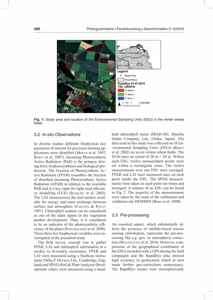
held chlorophyll meter (SPAD-502, Minolta Osaka Company, Ltd., Osaka, Japan). The data used in this study was collected on 18 En-vironmental Sampling Units (ESUs) (baret et al. 2002) on seven winter wheat fields. The EUSs have an extent of 20 m × 20 m. Within each ESU, twelve measurement points were set within a rectangular cross. The twelve measurements over one ESU were averaged. FPAR and LAI were measured once on each point inside the ESU. The SPAD measure-ments were taken on each point ten times and averaged. A scheme of an ESU can be found in Fig. 2. The majority of the measurements were taken by the team of the calibration and validation site DEMMIN (borg et al. 2009).

3.3 Pre-processing

An essential aspect, which substantially af-fects the accuracy of satellite-based remote sensing information, represents the pre-pro-cessing like e.g. geo- or atmospheric correc-tion (MannscHatz et al. 2014). However, com-parisons of the geographical coordinates of the ESUs recorded with a GPS during the field campaigns and the RapidEye data showed high accuracy in geolocation which in turn made further geo-corrections unnecessary. The RapidEye scenes were atmospherically

Fig. 1: Study area and location of the Environmental Sampling Units (ESU) in the winter wheat fields.


corrected and cloud masked using ATCOR2 (ricHter 2010).

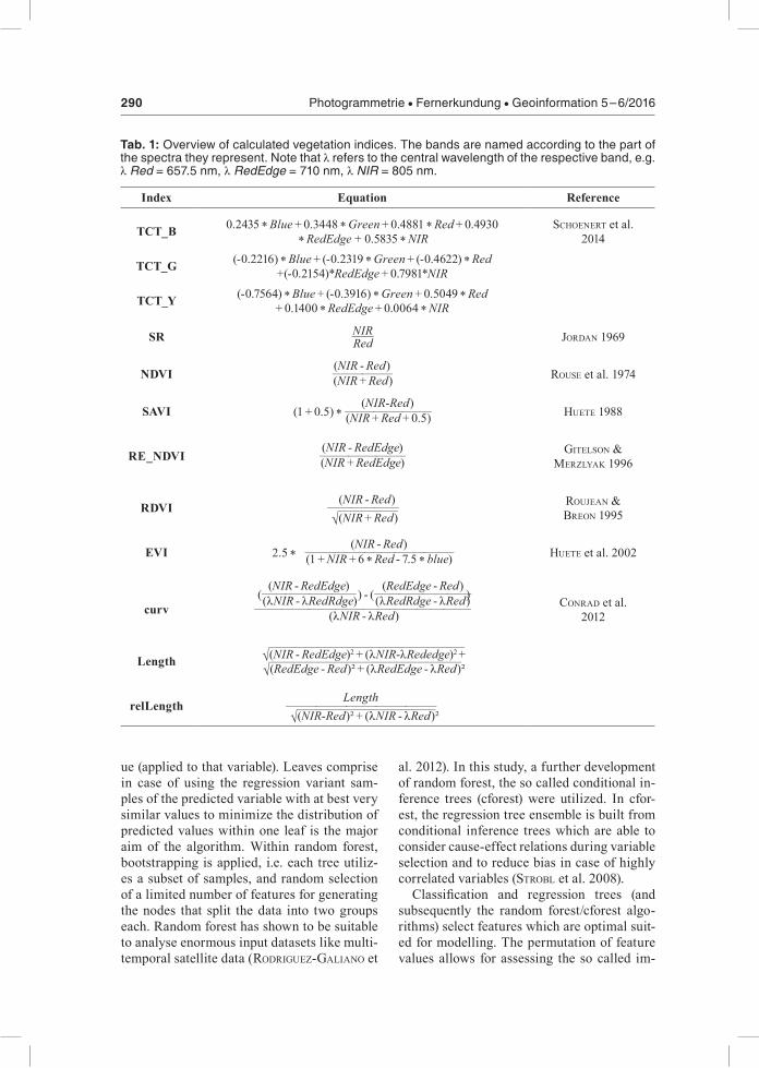
The reflectance spectrum of each RapidEye scene within all 18 ESUs was extracted by av-eraging RapidEye reflectance in a 20-meter radius around the centre of single ESU. This represents the spatial resolution of the new and upcoming Sentinel-2 Multi Spectral Instru-ment (MSI) data. Numerous vegetation indi-ces comprising SR, NDVI, SAVI, RE_NDVI, RDVI and EVI were calculated (Tab. 1). In ad-dition, the products of the tasselled cap trans-formation were included as they represent an-other important group of spectral indices in agriculture (scHoenert et al. 2014). With the additional RedEdge, the RapidEye system has been designed to derive information on the vegetation status (Jung-rotHenHäusler et al. 2007). Thus, different vegetation indices, which consider the RedEdge (RE_NDVI, rel-

Length, curve, Length; conrad et al. 2012) were also integrated in the feature set.

3.4 Phenological Groups

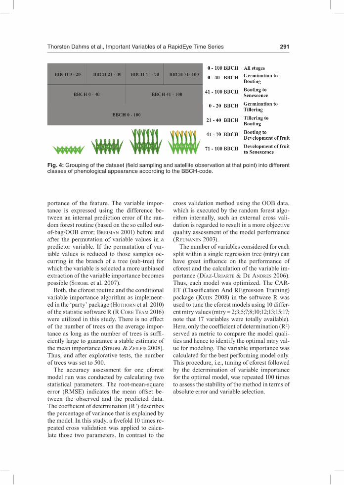
The second aim of this study was to investi-gate the variable importance of vegetation in-dices and single bands for the prediction of FPAR, LAI, and SPAD with respect to dif-ferent phenological stages. Therefore, each dataset was grouped according to the phenol-ogy using the BBCH-characterization (Biolo-gische Bundesanstalt, Bundessortenamt und CHemische Industrie) of the observation field data. The BBCH scale gives numeric informa-tion about the morphologic development stage of a plant (lancasHire et al. 1991). The groups were named after the BBCH range they cover. The grouping of the data is illustrated in Fig. 4. This step ensured that the spectral behav-iour was associated with the physical appear-ance of the plant and no longer with the data acquisition date. In other words, data pairs (field measurement and satellite observation at that point) were not analysed per data ac-quisition period, but within each phenological group.

3.5 Conditional Inference Forest

Random forests (breiMan 2001) are ensem-bles of classification and regression trees that operate on binary partitions of the feature space (drawn by the training samples). Each tree is built from nodes and leaves. Nodes consist of a predictor variable and a split val-

Fig. 2: ESU sampling scheme after GARRI-GUES et al. (2002).

Fig. 3: Overview about the data acquisition times in the field and the available RapidEye observa-tions.


ue (applied to that variable). Leaves comprise in case of using the regression variant sam-ples of the predicted variable with at best very similar values to minimize the distribution of predicted values within one leaf is the major aim of the algorithm. Within random forest, bootstrapping is applied, i.e. each tree utiliz-es a subset of samples, and random selection of a limited number of features for generating the nodes that split the data into two groups each. Random forest has shown to be suitable to analyse enormous input datasets like multi-temporal satellite data (rodriguez-galiano et

al. 2012). In this study, a further development of random forest, the so called conditional in-ference trees (cforest) were utilized. In cfor-est, the regression tree ensemble is built from conditional inference trees which are able to consider cause-effect relations during variable selection and to reduce bias in case of highly correlated variables (strobl et al. 2008).

Classification and regression trees (and subsequently the random forest/cforest algo-rithms) select features which are optimal suit-ed for modelling. The permutation of feature values allows for assessing the so called im-

Tab. 1: Overview of calculated vegetation indices. The bands are named according to the part of the spectra they represent. Note that λ refers to the central wavelength of the respective band, e.g. λ Red = 657.5 nm, λ RedEdge = 710 nm, λ NIR = 805 nm.

Index Equation Reference

TCT_B 0.2435 * Blue + 0.3448 * Green + 0.4881 * Red + 0.4930 * RedEdge + 0.5835 * NIR

scHoenert et al. 2014

TCT_G (-0.2216) * Blue + (-0.2319 * Green + (-0.4622) * Red +(-0.2154)*RedEdge + 0.7981*NIR

TCT_Y (-0.7564) * Blue + (-0.3916) * Green + 0.5049 * Red + 0.1400 * RedEdge + 0.0064 * NIR

SR NIR _ Red Jordan 1969

NDVI (NIR - Red)

__ (NIR + Red) rouse et al. 1974

SAVI (1 + 0.5) * (NIR-Red)

___ (NIR + Red + 0.5) Huete 1988

RE_NDVI (NIR - RedEdge)

___ (NIR + RedEdge) gitelson &

MerzlyaK 1996

RDVI (NIR - Red)

___

√__________

(NIR + Red) rouJean &

breon 1995

EVI 2.5 * (NIR - Red)

_____ (1 + NIR + 6 * Red - 7.5 * blue) Huete et al. 2002

curv (

(NIR - RedEdge) ____ (λNIR - λRedRdge) ) - (

(RedEdge - Red) ____ (λRedRdge - λRed) ) ________ (λNIR - λRed) conrad et al.

2012

Length √________________________________

(NIR - RedEdge)2 + (λNIR-λRededge)2 +

√________________________________

(RedEdge - Red)² + (λRedEdge - λRed)²

relLength Length

_____

√_______________________

(NIR-Red)² + (λNIR - λRed)²


cross validation method using the OOB data, which is executed by the random forest algo-rithm internally, such an external cross vali-dation is regarded to result in a more objective quality assessment of the model performance (reunanen 2003).

The number of variables considered for each split within a single regression tree (mtry) can have great influence on the performance of cforest and the calculation of the variable im-portance (díaz-uriarte & de andres 2006). Thus, each model was optimized. The CAR-ET (Classification And REgression Training) package (KuHn 2008) in the software R was used to tune the cforest models using 10 differ-ent mtry values (mtry = 2;3;5;7;8;10;12;13;15;17; note that 17 variables were totally available). Here, only the coefficient of determination (R2) served as metric to compare the model quali-ties and hence to identify the optimal mtry val-ue for modeling. The variable importance was calculated for the best performing model only. This procedure, i.e., tuning of cforest followed by the determination of variable importance for the optimal model, was repeated 100 times to assess the stability of the method in terms of absolute error and variable selection.

portance of the feature. The variable impor-tance is expressed using the difference be-tween an internal prediction error of the ran-dom forest routine (based on the so called out-of-bag/OOB error; breiMan 2001) before and after the permutation of variable values in a predictor variable. If the permutation of var-iable values is reduced to those samples oc-curring in the branch of a tree (sub-tree) for which the variable is selected a more unbiased extraction of the variable importance becomes possible (strobl et al. 2007).

Both, the cforest routine and the conditional variable importance algorithm as implement-ed in the ‘party’ package (HotHorn et al. 2010) of the statistic software R (R core teaM 2016) were utilized in this study. There is no effect of the number of trees on the average impor-tance as long as the number of trees is suffi-ciently large to guarantee a stable estimate of the mean importance (strobl & zeileis 2008). Thus, and after explorative tests, the number of trees was set to 500.

The accuracy assessment for one cforest model run was conducted by calculating two statistical parameters. The root-mean-square error (RMSE) indicates the mean offset be-tween the observed and the predicted data. The coefficient of determination (R2) describes the percentage of variance that is explained by the model. In this study, a fivefold 10 times re-peated cross validation was applied to calcu-late those two parameters. In contrast to the

Fig. 4: Grouping of the dataset (field sampling and satellite observation at that point) into different classes of phenological appearance according to the BBCH-code.


4.2 Variable Importance

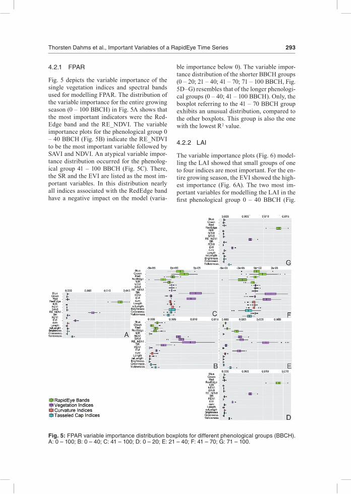
The cforest based variable importance for modelling the biophysical parameters (FPAR, LAI and SPAD) in every BBCH-based pheno-logical group can be seen in Figs. 5 to 7. The boxplots show the unscaled variable impor-tance for each of the 17 indices or bands re-ceived during all 100 model runs for one pa-rameter and phenological group. The boxplots allow for comparing the variable importance of indices or bands used for modelling. High variable importance indicates an increase of the prediction error in cforest when the re-spective band or index is excluded. On the contrary, small or negative variable impor-tance shows that omitting the tested band or index from cforest has none or negative im-pact on the model accuracy. The distribution of variable importance scores of the 100 mod-el runs determines the size of the boxes, which in turn puts a light on the stability of the im-portance level of each index or band during modelling. For instance, a slim box indicates a more stable importance estimation of the re-spective index or band, a broad box suggest varying importance levels (relevance) of that variable over numerous runs.

4 Results

4.1 Prediction Accuracy

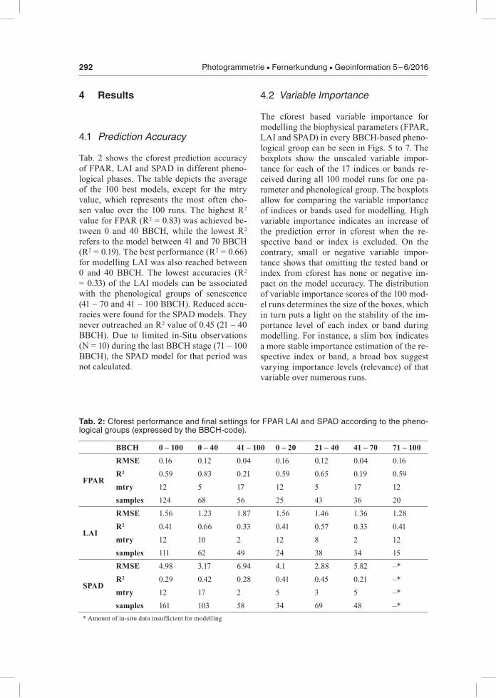
Tab. 2 shows the cforest prediction accuracy of FPAR, LAI and SPAD in different pheno-logical phases. The table depicts the average of the 100 best models, except for the mtry value, which represents the most often cho-sen value over the 100 runs. The highest R2 value for FPAR (R2 = 0.83) was achieved be-tween 0 and 40 BBCH, while the lowest R2 refers to the model between 41 and 70 BBCH (R2 = 0.19). The best performance (R2 = 0.66) for modelling LAI was also reached between 0 and 40 BBCH. The lowest accuracies (R2 = 0.33) of the LAI models can be associated with the phenological groups of senescence (41 – 70 and 41 – 100 BBCH). Reduced accu-racies were found for the SPAD models. They never outreached an R2 value of 0.45 (21 – 40 BBCH). Due to limited in-Situ observations (N = 10) during the last BBCH stage (71 – 100 BBCH), the SPAD model for that period was not calculated.

Tab. 2: Cforest performance and final settings for FPAR LAI and SPAD according to the pheno-logical groups (expressed by the BBCH-code).

BBCH 0 – 100 0 – 40 41 – 100 0 – 20 21 – 40 41 – 70 71 – 100

FPAR

RMSE 0.16 0.12 0.04 0.16 0.12 0.04 0.16R2 0.59 0.83 0.21 0.59 0.65 0.19 0.59mtry 12 5 17 12 5 17 12samples 124 68 56 25 43 36 20

LAI

RMSE 1.56 1.23 1.87 1.56 1.46 1.36 1.28R2 0.41 0.66 0.33 0.41 0.57 0.33 0.41mtry 12 10 2 12 8 2 12samples 111 62 49 24 38 34 15

SPAD

RMSE 4.98 3.17 6.94 4.1 2.88 5.82 –*R2 0.29 0.42 0.28 0.41 0.45 0.21 –*mtry 12 17 2 5 3 5 –*samples 161 103 58 34 69 48 –*

* Amount of in-situ data insufficient for modelling


ble importance below 0). The variable impor-tance distribution of the shorter BBCH groups (0 – 20; 21 – 40; 41 – 70; 71 – 100 BBCH, Fig. 5D–G) resembles that of the longer phenologi-cal groups (0 – 40; 41 – 100 BBCH). Only, the boxplot referring to the 41 – 70 BBCH group exhibits an unusual distribution, compared to the other boxplots. This group is also the one with the lowest R2 value.

4.2.2 LAI

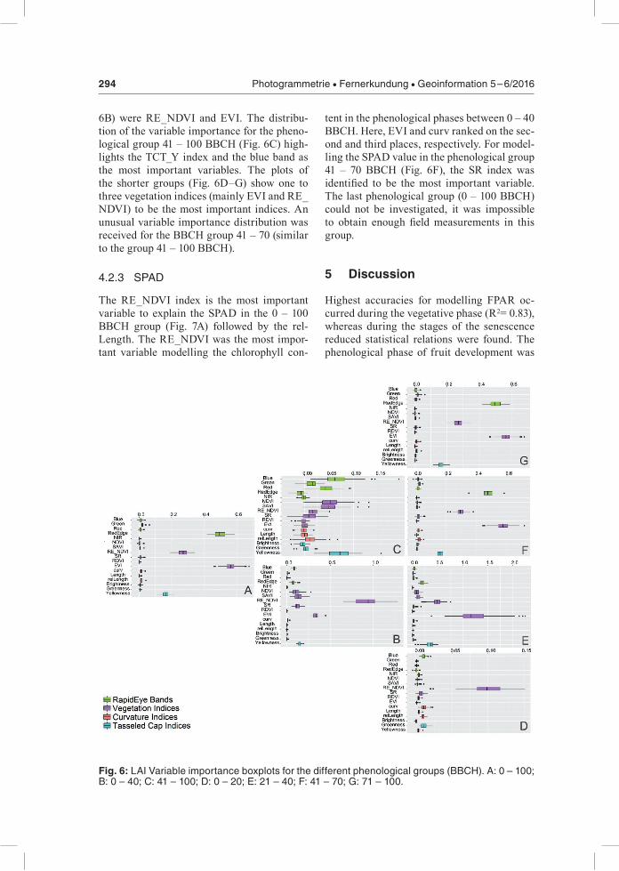
The variable importance plots (Fig. 6) model-ling the LAI showed that small groups of one to four indices are most important. For the en-tire growing season, the EVI showed the high-est importance (Fig. 6A). The two most im-portant variables for modelling the LAI in the first phenological group 0 – 40 BBCH (Fig.

4.2.1 FPAR

Fig. 5 depicts the variable importance of the single vegetation indices and spectral bands used for modelling FPAR. The distribution of the variable importance for the entire growing season (0 – 100 BBCH) in Fig. 5A shows that the most important indicators were the Red-Edge band and the RE_NDVI. The variable importance plots for the phenological group 0 – 40 BBCH (Fig. 5B) indicate the RE_NDVI to be the most important variable followed by SAVI and NDVI. An atypical variable impor-tance distribution occurred for the phenolog-ical group 41 – 100 BBCH (Fig. 5C). There, the SR and the EVI are listed as the most im-portant variables. In this distribution nearly all indices associated with the RedEdge band have a negative impact on the model (varia-

Fig. 5: FPAR variable importance distribution boxplots for different phenological groups (BBCH). A: 0 – 100; B: 0 – 40; C: 41 – 100; D: 0 – 20; E: 21 – 40; F: 41 – 70; G: 71 – 100.


tent in the phenological phases between 0 – 40 BBCH. Here, EVI and curv ranked on the sec-ond and third places, respectively. For model-ling the SPAD value in the phenological group 41 – 70 BBCH (Fig. 6F), the SR index was identified to be the most important variable. The last phenological group (0 – 100 BBCH) could not be investigated, it was impossible to obtain enough field measurements in this group.

5 Discussion

Highest accuracies for modelling FPAR oc-curred during the vegetative phase (R2= 0.83), whereas during the stages of the senescence reduced statistical relations were found. The phenological phase of fruit development was

6B) were RE_NDVI and EVI. The distribu-tion of the variable importance for the pheno-logical group 41 – 100 BBCH (Fig. 6C) high-lights the TCT_Y index and the blue band as the most important variables. The plots of the shorter groups (Fig. 6D–G) show one to three vegetation indices (mainly EVI and RE_NDVI) to be the most important indices. An unusual variable importance distribution was received for the BBCH group 41 – 70 (similar to the group 41 – 100 BBCH).

4.2.3 SPAD

The RE_NDVI index is the most important variable to explain the SPAD in the 0 – 100 BBCH group (Fig. 7A) followed by the rel-Length. The RE_NDVI was the most impor-tant variable modelling the chlorophyll con-

Fig. 6: LAI Variable importance boxplots for the different phenological groups (BBCH). A: 0 – 100; B: 0 – 40; C: 41 – 100; D: 0 – 20; E: 21 – 40; F: 41 – 70; G: 71 – 100.


nearby impossible to model with high accu-racy (R2 = 0.19), most likely due to canopy clo-sure in combination with accompanied satu-ration effects in the RapidEye observations. The challenges modelling FPAR during the saturation or senescence phase is also high-lighted by the by the variable importance dis-tribution: While the variable importance of the initial growing stages shows three indices RE_NDVI, NDVI and SAVI to be the most important ones, the only vague patterns of variable importance were observed during the fruit development and the senescence phases. For the latter, the importance values were gen-erally smaller and no group of important indi-ces with distinct spectral properties emerged during analysis.

In comparison to FPAR only slightly re-duced modelling accuracies were found when modelling the LAI. The accuracy levels were comparable with the accuracies zHao et al. (2015), who modelled the LAI of wheat us-ing univariate regressions and the HJ-1 sensor system and achieved a R2 of 0.58 and RMSE values ranging from 0.7 to 0.89. However, in

contrast to the FPAR results the variable im-portance plots for LAI indicate a more distinct distribution among the detailed phenological groups. There, a group of one to four indices were found to be most important for the cfor-est model. The observation that EVI is the highest ranked index among the phenological stages of growth, fruit development and se-nescence can be explained by a higher robust-ness of that index against saturation effects that occur in these phenological phases due to the closed canopy (Huete et al. 2002).

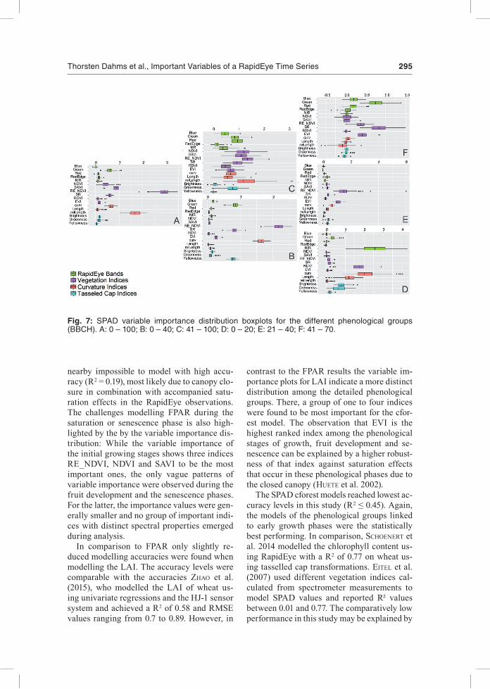
The SPAD cforest models reached lowest ac-curacy levels in this study (R2 ≤ 0.45). Again, the models of the phenological groups linked to early growth phases were the statistically best performing. In comparison, scHoenert et al. 2014 modelled the chlorophyll content us-ing RapidEye with a R2 of 0.77 on wheat us-ing tasselled cap transformations. eitel et al. (2007) used different vegetation indices cal-culated from spectrometer measurements to model SPAD values and reported R² values between 0.01 and 0.77. The comparatively low performance in this study may be explained by

Fig. 7: SPAD variable importance distribution boxplots for the different phenological groups (BBCH). A: 0 – 100; B: 0 – 40; C: 41 – 100; D: 0 – 20; E: 21 – 40; F: 41 – 70.


The variable importance varied among the biophysical parameters and the phenological stages, which in turn indicates a link with the physical appearance of wheat during the crop-ping season. Nevertheless, altogether, the RE_NDVI or the RDVI were found to be the most important variables which in turns underlines the importance of RedEdge bands for model-ling biophysical parameters of crops, at least those of winter wheat.

Cforest was applied to one ensemble of veg-etation indices and single bands of the Rapid-Eye system. Even though some features re-peatedly showed high variable importance, the results may have varied in case other sen-sor systems, e.g. Sentinel-2, acquisition dates, or spectral features have been included. Such considerations have to be taken into account in further research and discussions about the transferability of the approach. Nevertheless, indication for the selection of the important features is given, because wheat represents a single plant type with a closed canopy. This information can in turn contribute to reduce the computation efforts, which is of para-mount importance with a look on the continu-ously increasing data amount at the high reso-lution remote sensing sector.

Acknowledgements

We express our gratitude to the team of the Calibration and Validation Facility DEMMIN of the German Aerospace Center (DLR) who commonly conducted the field observations throughout the vegetation period accompa-nied by students of the University of Würz-burg. The Blackbridge Company (RESA Pro-ject 0028) provided the RapidEye data for this study. The Federal Ministry of Economic Af-fairs and Energy funded this research (FKZ: 50 EE 1353).

the temporal offset between the in situ obser-vation and the satellite data acquisition of four days which may be too long for modelling a bi-ophysical parameter like chlorophyll content. The RedEdge band and related indices always ranked under the most important variables for the prediction of SPAD values. This confirms the usefulness of analysing chlorophyll con-tent in the RedEdge spectra as demonstrated previously (eitel et al. 2007). The observation that spectral curvature indices can contribute to successful modelling of chlorophyll content is in line with the results presented by eitel et al. (2007) based on simulated RapidEye and hyperspectral data for wheat.

6 Conclusion

Remote sensing applications for farmers like precision farming demand up to date informa-tion on the crop in specific phenological phas-es. Several field management methods like the application of fertilizers depend on the phe-nological phase of the plant. This study ad-dressed the utility of RapidEye data and the use of machine learning for obtaining growth information about winter wheat in different phenological stages and to show how the vari-able importance changes along with the phe-nology. Thereby, the cforest was found suit-able to model biophysical parameters for the entire growing season and to get an increased understanding about variables useful for pre-dictions. Several vegetation indices were iden-tified to be very important for the derivation of the biophysical parameters FPAR, LAI and chlorophyll content (approximated with the SPAD-value).

The model performance for the entire grow-ing season outreached that for single pheno-logical groups. There, the vegetative phase (0 – 40 BBCH) showed the best performance and more stable variable importance distribution, particular in contrast to the senescence phase (70 – 100 BBCH). Models with a high accu-racy relied on a small set of input parameters only. The latter may allow for questioning the use of more complex approaches to model bio-physical parameters of winter wheat and crops with similar physical appearance (e.g. other cereal crops).


2013: Radiometric and geometric assessment of data from the RapidEye constellation of satel-lites. – International Journal of Remote Sensing 34 (16): 5905–5925.

conrad, c., FritscH, s., leX, s., loeW, F., ruecKer, g., scHorcHt, g. & laMers, J., 2012: Potenziale des Red Edge Kanals von RapidEye zur Unter-scheidung und zum Monitoring landwirtschaftli-cher Anbaufrüchte am Beispiel des usbekischen wässerungssystems Khorezm. – borg, e., daedeloW, H. & JoHnson, r. (eds.): RapidEye Science Archive (RESA) – Vom Algorithmus zum Produkt, 4. RESA Workshop (pp. 203–217). – GITO, Berlin.

darVisHzadeH, r., sKidMore, a., scHlerF, M. & atzberger, c., 2008: Inversion of a radiative transfer model for estimating vegetation LAI and chlorophyll in a heterogeneous grassland. – Remote Sensing of Environment 112 (5): 2592–2604.

díaz-uriarte, r. & de andres, s.a., 2006: Gene selection and classification of microarray data using random forest. – BioMed Central Bioin-formatics 7 (1): 1.

dong, t., Meng, J. & Wu, b., 2012: Overview on methods of deriving fraction of absorbed photo-synthetically active radiation (FPAR) using re-mote sensing. – Shengtai Xuebao/Acta Ecologi-ca Sinica 32 (22): 7190–7201.

eitel, J.u.H., long, d.s., gessler, P.e. & sMitH, a.M.s., 2007: Using in- situ measurements to evaluate the new RapidEy satellite series for pre-diction of wheat nitrogen status. – International Journal of Remote Sensing 28 (18): 4183–4190.

FranKe, J. & Menz, G., 2007: Multi-temporal wheat disease detection by multi-spectral remote sens-ing. – Precision Agriculture 8 (3): 161–172.

garrigues, s., allard, d., Weiss, M. & baret, F., 2002: Comparing VALERI sampling schemes to better represent high spatial resolution satellite pixel from ground measurements: How to char-acterize an ESU. – http://w3.avignon.inra.fr/valeri/methodology/samplingschemes.pdf (19.10.2016).

gerigHausen, H., borg, e., FicHtelMann, b., guen-tHer, a., VaJen, H.H., WloczyK, c., Maass, H., 2009: Validation and calibration of remote sens-ing data products on test site DEMMIN. – 43. Ziolkowski Conference (pp. 18–33). – Russische Akademie der Wissenschaften.

gitelson, a.a. & MerzlyaK, M., 1996: Signature analysis of leaf reflectance spectra: algorithm development for remote sensing of chlorophyll. – Journal of Plant Physiology 148 (3): 494–500.

Haboudane, d., Miller, J.r., Pattey, e., zarco-teJada, P.J. & stracHan, i.b., 2004: Hyperspec-tral vegetation indices and novel algorithms for

References

aHMadian, n., gHaseMi, s., Wigneron, J.P. & zoe-litz, R., 2016: Comprehensive study of the bio-physical parameters of agricultural crops based on assessing Landsat 8 OLI and Landsat 7 ETM+ vegetation indices. – GIScience & Remote Sens-ing 53 (3): 337–359.

baret, F., Houles, V. & gueriF, M., 2007: Quantifi-cation of plant stress using remote sensing ob-servations and crop models: the case of nitrogen management. – Journal of Experimental Botany 58 (4): 869–880.

becKscHaeFer, P., FeHrMann, l., Harrison, r.d., Xu, J. & Kleinn, c., 2014:. Mapping Leaf Area Index in subtropical upland ecosystems using RapidEye imagery and the randomForest algo-rithm. – iForest-Biogeosciences and Forestry 7 (1): 1.

bonteMPs, s., arias, M., cara, c., dedieu, g., guz-zonato, e., Hagolle, o., inglada, J., Matton, n., Morin, d., PoPescu, r., rabaute, t., saVinaud, M., sePulcre, g., Valero, s., aHMad, i., bégué, a., Wu, b., abelleyra, d., diarra, a., duPui, s., FrencH, a., aKHtar, i., Kussul, n., lebourgeois, V., le Page, M., neWby, t., saVin, i., Verón, s., Koetz, b. & deFourny, P., 2015: Building a data set over 12 globally distributed sites to support the development of agriculture monitoring ap-plications with Sentinel-2. – Remote Sensing 7 (12): 16062–16090.

borg, e., liPPert, K., zabel, e., loePMeier, F.J., FicHtelMann, b., JaHncKe, d. & Maass, H., 2009: deMMin – Teststandort zur Kalibrierung und Validierung von Fernerkundungsmissionen. – rebenstorF, R.W. (Hrsg.): 15 Jahre Studiengang Vermessungswesen – Geodätisches Fachforum und Festakt, Neubrandenburg, Eigenverlag: 401–419.

borg, e., daedeloW, H., Missling, K.-d. & aPel, M., 2013: RapidEye Science Archive: Remote Sensing Data for the German Scientific Commu-nity. – borg, e., daedeloW, H. & JoHnson, r. (eds.): 5th RESA Workshop “Data for Science: From the Basics to the Service”: 5–20, Neustre-litz, 20.–21.3.2012, GITO mbH Verlag, Berlin, ISBN 978-3-95545-002-1.

breiMan, l., 2001: Random forests. – Machine Learning 45 (1): 5–32.

carlson, t. & riPley, d., 1997: On the relation be-tween NDVI, fractional vegetation cover, and leaf area index. – Remote Sensing of Environ-ment 62 (3): 241–252.

cHander, g., Haque, M.o., saMPatH, a., brunn, a., trosset, g., HoFFMann, d. & anderson, C.,


leX, s., conrad, c. & scHorcHt, g., 2013: Analyz-ing the seasonal relations between in situ fpar/LAI of cotton and spectral information of Rapid-Eye. – borg, e., daedeloW, H. & JoHnson, r. (eds.): RapidEye Science Archive (RESA) – From the Basics to the Service. – GITO, Berlin.

leX, s., asaM, s., löW, F. & conrad, c., 2015: Comparison of two Statistical Methods for the Derivation of the Fraction of Absorbed Photo-synthetic Active Radiation for Cotton. – PFG – Photogrammetrie, Fernerkundung, Geoinforma-tion 2015 (1): 55–67.

MannscHatz, t., PFlug, b., borg, e., Feger, K.H. & dietricH, P., 2014: Uncertainties of LAI esti-mation from satellite imaging due to atmospher-ic correction. – Remote Sensing of Environment 153: 24–39.

Moran, M.s., inoue, y. & barnes, e.M., 1997: Op-portunities and limitations for image-based re-mote sensing in precision crop management. – Remote sensing of Environment 61 (3): 319–346.

Mutanga, o., adaM, e. & cHo, M.a., 2012: High density biomass estimation for wetland vegeta-tion using WorldView-2 imagery and random forest regression algorithm. – International Jour-nal of Applied Earth Observation and Geoinfor-mation 18: 399–406.

Mutanga, o. & sKidMore, a.K., 2004: Narrow band vegetation indices overcome the saturation problem in biomass estimation. – International Journal of Remote Sensing 25 (19): 3999–4014.

Myneni, r.b. & WilliaMs, d.l., 1994: On the rela-tionship between FAPAR and NDVI. – Remote Sensing of Environment 49 (3): 200–211.

r core teaM (2014). R: A language and environ-ment for statistical computing. – R Foundation for Statistical Computing, Vienna, Austria. URL http://www.R-project.org/ (20.10.2016).

reunanen, J., 2003: Overfitting in making com-parisons between variable selection methods. – Journal of Machine Learning Research 3: 1371–1382.

ricHter, r. (2010). Atmospheric/Topographic Cor-rection for Satellite Imagery (ATCOR-2/3 User Guide, Version 7.1, January 2008), 165.

rodriguez-galiano, V.F., gHiMire, b., rogan, J., cHica-olMo, M. & rigol-sancHez, J.P., 2012: An assessment of the effectiveness of a random forest classifier for land-cover classification. – ISPRS Journal of Photogrammetry and Remote Sensing 67: 93–104.

rouJean, J.l. & breon, F.M., 1995: Estimating PAR absorbed by vegetation from bidirectional reflectance measurements. – Remote Sensing of Environment 51 (3): 375–384.

rouse, J.W., Haas, r.H., scHell, J.a., deering, d.W. & Harlan, J.c, 1974: Monitoring the ver-

predicting green LAI of crop canopies: Mode-ling and validation in the context of precision agriculture. – Remote Sensing of Environment 90 (3): 337–352.

Hall, F.g., toWnsHend, J.r. & engMan, e.t., 1995: Status of remote sensing algorithms for estima-tion of land surface state parameters. – Remote Sensing of Environment 51 (1): 138–156.

HGF, 2015: TERENO Northeastern German Low-land Observatory. – http://teodoor.icg.kfa-juelich.de/observatories/GL_Observatory?set_language=en (8.5.2016).

HotHorn, t., bueHlMann, P., Kneib, t., scHMid, M. & HoFner, B., 2010: Model-based boosting 2.0. – Journal of Machine Learning Research 11: 2109–2113.

Huete, a., didan, K., Miura, t., rodriguez, e.P., gao, X. & Ferreira, l.g., 2002: Overview of the radiometric and biophysical performance of the MODIS vegetation indices. – Remote Sens-ing of Environment 83 (1): 195–213.

Huete, a., 1988: A soil-adjusted vegetation index (SAVI). – Remote Sensing of Environment 25 (3): 295–309.

Jin, X.l., diao, W.y., Xiao, c.H., Wang, F.y., cHen, b., Wang, K.r. & li, s.K., 2013: Estimation of wheat agronomic parameters using new spectral indices. – PLOS ONE 8: e72736 doi: 10.1371/journal.pone.0072736

Jordan, c.F., 1969: Derivation of leaf are index from quality of light on the forest floor. – Ecolo-gy 50: 663–666.

Jung-rotHenHäusler, F., WeicHelt, H. & PacH, M., 2007: RapidEye. A novel approach to space borne geo-information solutions. – International Society for Photogrammetry and Remote Sens-ing, Hanover Workshop, 29.05. – 01.06.2017.

Kross, a., Mcnairn, H., laPen, d., sunoHara, M. & cHaMPagne, c., 2015: Assessment of RapidEye vegetation indices for estimation of leaf area in-dex and biomass in corn and soybean crops. – International Journal of Applied Earth Observa-tion and Geoinformation 34: 235–248.

KuHn, M., 2008: Building predictive models in R using the caret package. – Journal of Statistical Software 28 (5).

lancasHire, P.d., bleiHolder, H., langelueddecKe, P., stauss, r., Van den booM, t., Weber, e. & Witzenberger, a., 1991: An uniform decimal code for growth stages of crops and weeds. – Annals of Applied Biology 119: 561–601.

le Maire, g., Marsden, c., VerHoeF, W., Ponzoni, F.J., seen, d.l., bégué, a. & nouVellon, y., 2011: Leaf area index estimation with MODIS reflectance time series and model inversion dur-ing full rotations of Eucalyptus plantations. – Re-mote Sensing of Environment 115 (2): 586–599.


Viña, A., Gitelson, A.A., Nguy-Robertson, A.L. & Peng, Y., 2011: Comparison of different vegeta-tion indices for the remote assessment of green leaf area index of crops. – Remote Sensing of Environment 115 (12): 3468–3478.

zHao, J., li, J., liu, q., Fan, W., zHong, b., Wu, s. & yin, g., 2015: Leaf area index retrieval com-bining HJ1/CCD and Landsat8/OLI data in the Heihe River Basin, China. – Remote Sensing 7 (6): 6862–6885.

Addresses of the authors:

tHorsten daHMs, sylVia seissiger & cHristoPHer conrad, Julius Maximilians University Würzburg, Institut für Geographie und Geologie, Lehrstuhl für Fernerkundung, Campus Hubland Nord 86, D-97074 Würzburg; e-mail: {thorsten.dahms}{sylvia.seissiger}{christopher.conrad}@uni-wuerzburg.de

eriK borg, VaJen Hans-HerMann & bernd FicHtel-Man, German Remote Sensing Data Center, National Ground Segment, Kalkhorstweg 53, D-17235 Neu-strelitz; e-mail: {erik.borg}{hans-hermann.vajen} {bernd.fichtelmann}@dlr.de

Manuskript eingereicht: September 2016Angenommen: Oktober 2016

nal advancement of retrogradiation of natural vegetation. – NASA/GSFC, Type III, Final Re-port: 371, Greenbelt, MD, USA.

scHoenert, M., WeicHelt, H., zillMann, e. & Juer-gens, c., 2014: Derivation of tasseled cap coeffi-cients for RapidEye data. – SPIE 9245, Earth Resources and Environmental Remote Sensing/GIS Applications V, 92450Q (October 23, 2014); doi: 10.1117/12.2066842.

seaquist, J.W., olsson, l. & ardoe, J., 2003: A re-mote sensing-based primary production model for grassland biomes. – Ecological Modelling 169 (1): 131–155.

strobl, c., boulesteiX, a.l., Kneib, t., augustin, t. & zeileis, a., 2008: Conditional variable im-portance for random forests. – BioMed Central Bioinformatics 9 (1): 25; doi: 10.1186/1471-2105-9-307.

strobl, c., boulesteiX, a.l., zeileis, a. & Ho-tHorn, t., 2007: Bias in random forest variable importance measures – Illustrations, sources and a solution. – BioMed Central Bioinformatics 8 (1): 307; doi: 10.1186/1471-2105-8-25.

strobl, c. & zeileis, a., 2008: Danger: high power!-exploring the statistical properties of a test for random forest variable importance. – Technical Report Number 017, 2008, Department of Statis-tics University of Munich, Munich.

tillacK, a., clasen, a., KleinscHMit, b. & Foers-ter, M., 2014: Estimation of the seasonal leaf area index in an alluvial forest using high-reso-lution satellite-based vegetation indices. – Re-mote Sensing of Environment 141: 52–63.

Documents

Important Variables of a RapidEye Time Series for ... · Thorsten Dahms et al., Important Variables of a RapidEye Time Series 287 spectral indices or band selection can be use-ful