Improved accuracy for fluid flow problems via enhancedphysics

A ThesisPresented to

the Graduate School ofClemson University

In Partial Fulfillmentof the Requirements for the Degree

Doctor of PhilosophyMathematical Sciences

byMichael A. Case

May 2010

Accepted by:Dr. Leo Rebholz, Committee Chair

Dr. Eleanor Jenkins, Co-ChairDr. Chris CoxDr. Nigel Kaye

This thesis is an investigation of numerical methods for approximating solutions to fluid

flow problems, specifically the Navier-Stokes equations (NSE) and magnetohydrodynamic equations

(MHD), with an overriding theme of enforcing more physical behavior in discrete solutions. It is

well documented that numerical methods with more physical accuracy exhibit better long-time

behavior than comparable methods that enforce less physics in their solutions. This work develops,

analyzes and tests finite element methods that better enforce mass conservation in discrete velocity

solutions to the NSE and MHD, helicity conservation for NSE, cross-helicity conservation in MHD,

and magnetic field incompressibility in MHD.

ii

Table of Contents

Title Page . . . . . . . . . . . . . . . . . . . . . . . . . . . . . . . . . . . . . . . . . . . i

Abstract . . . . . . . . . . . . . . . . . . . . . . . . . . . . . . . . . . . . . . . . . . . . ii

List of Tables . . . . . . . . . . . . . . . . . . . . . . . . . . . . . . . . . . . . . . . . . iv

List of Figures . . . . . . . . . . . . . . . . . . . . . . . . . . . . . . . . . . . . . . . . v

1 Introduction . . . . . . . . . . . . . . . . . . . . . . . . . . . . . . . . . . . . . . . . 1

2 Scott-Vogelius Elements . . . . . . . . . . . . . . . . . . . . . . . . . . . . . . . . 4

3 Stable computing with an enhanced physics based scheme for the 3d Navier-Stokes equations . . . . . . . . . . . . . . . . . . . . . . . . . . . . . . . . . . . . . 213.1 Introduction . . . . . . . . . . . . . . . . . . . . . . . . . . . . . . . . . . . . . . . . . 213.2 Mathematical Preliminaries . . . . . . . . . . . . . . . . . . . . . . . . . . . . . . . . 233.3 Stability, conservation laws, and existence of solutions . . . . . . . . . . . . . . . . . 263.4 Convergence . . . . . . . . . . . . . . . . . . . . . . . . . . . . . . . . . . . . . . . . . 313.5 Numerical Experiments . . . . . . . . . . . . . . . . . . . . . . . . . . . . . . . . . . 403.6 Conclusions and future directions . . . . . . . . . . . . . . . . . . . . . . . . . . . . . 42

4 Improving mass conservation in FE approximations of the Navier Stokes equa-tions using C0 velocity fields: A connection between grad-div stabilization andScott-Vogelius elements . . . . . . . . . . . . . . . . . . . . . . . . . . . . . . . . . 454.1 Introduction . . . . . . . . . . . . . . . . . . . . . . . . . . . . . . . . . . . . . . . . . 454.2 Preliminaries . . . . . . . . . . . . . . . . . . . . . . . . . . . . . . . . . . . . . . . . 484.3 A relation between the Taylor-Hood and the Scott-Vogelius element . . . . . . . . . 524.4 2D Numerical Experiments . . . . . . . . . . . . . . . . . . . . . . . . . . . . . . . . 564.5 Conclusions and Future Directions . . . . . . . . . . . . . . . . . . . . . . . . . . . . 61

5 An enhanced physics numerical scheme for MHD . . . . . . . . . . . . . . . . . 655.1 Introduction . . . . . . . . . . . . . . . . . . . . . . . . . . . . . . . . . . . . . . . . . 655.2 Notation and Preliminaries . . . . . . . . . . . . . . . . . . . . . . . . . . . . . . . . 675.3 Derivation of energy and cross-helicity conserving scheme . . . . . . . . . . . . . . . 695.4 Numerical analysis of the scheme . . . . . . . . . . . . . . . . . . . . . . . . . . . . . 72

iii

List of Tables

2.1 Sample Problem Velocity Error, ν = 1.0.. . . . . . . . . . . . . . . . . . . . . . . . . 82.2 Sample Problem Velocity Error, ν = 1.0. w/Pres. Stab., ε = 1.0e-6. . . . . . . . . . . 9

3.1 The ‖|uNSE − uh|‖2,1 errors and experimental convergence rates for each of the threescheme of Algorithm 3.2.1. . . . . . . . . . . . . . . . . . . . . . . . . . . . . . . . . . 41

4.1 The table above shows convergence of the grad-div stabilized TH approximations tothe SV approximation for numerical experiment 1. . . . . . . . . . . . . . . . . . . . 57

4.2 Convergence of the grad-div stabilized TH approximations toward the SV approxi-mation as γ →∞ for the Re = 100 3d driven cavity problem. . . . . . . . . . . . . . 61

iv

List of Figures

2.1 (LEFT) 2D and (RIGHT) 3D Clough-Tocher macro-element, shown with dashedlines representing barycenter refinements . . . . . . . . . . . . . . . . . . . . . . . . . 6

2.2 (LEFT) 2D conforming mesh and (RIGHT) mesh resulting from barycentric refine-ment. . . . . . . . . . . . . . . . . . . . . . . . . . . . . . . . . . . . . . . . . . . . . 7

2.3 Shown above is the mesh used for the flow around a cylinder computations in thisexperiment. . . . . . . . . . . . . . . . . . . . . . . . . . . . . . . . . . . . . . . . . . 11

2.4 Shown above are the t=7 velocity fields, speed contours, and pressure contours plotsfor solution obtained using Scott-Vogelius elements (top) Taylor-Hood elements (bot-tom). . . . . . . . . . . . . . . . . . . . . . . . . . . . . . . . . . . . . . . . . . . . . . 14

2.5 Shown above are the plots of ‖∇ · unh‖ vs. time for the SV and TH solutions for the2D cylinder problem. . . . . . . . . . . . . . . . . . . . . . . . . . . . . . . . . . . . . 15

2.6 The barycenter-refined mesh used for the 2D step computations . . . . . . . . . . . . 152.7 For SV elements the flow profile appears to agree with the “true” solution[32]. . . . 162.8 For TH elements the velocity field is underresolved and fails to shed eddies at T = 40. 172.9 Shown above are the plots of ‖∇ · unh‖ vs. time for the SV and TH solutions for the

2D step problem. . . . . . . . . . . . . . . . . . . . . . . . . . . . . . . . . . . . . . . 182.10 The barycenter-refined mesh used for the 3D lid-driven cavity problem. . . . . . . . 192.11 3D lid-driven cavity results with SV elements. Note the small scale next to the color

bar. . . . . . . . . . . . . . . . . . . . . . . . . . . . . . . . . . . . . . . . . . . . . . 192.12 3D lid-driven cavity results with TH elements. Note the scale next to the color bar

and the contours in the corners of each midplane. . . . . . . . . . . . . . . . . . . . . 202.13 3D lid-driven cavity results compared to “true” solution on centerline. . . . . . . . . 20

3.1 The velocity solution to the Ethier-Steinman problem with a = 1.25, d = 1 at t = 0on the (−1, 1)3 domain. The complex flow structure is seen in the streamribbons inthe box and the velocity streamlines and speed contours on the sides. . . . . . . . . 40

3.2 The plot above shows L2 error of the velocity vs time for the four schemes of Test2. We see in the plot that the stabilizations add accuracy to the enhanced-physicsscheme, and that the alternate grad-div stabilization gives slightly better resultsthan the usual grad-div stabilization. It can also be seen that the enhanced-physicsscheme is far more accurate in this metric than the usual CCN scheme. . . . . . . . 43

3.3 The plot above shows helicity error vs time for the four schemes of Test 2. We see inthe plot that helicity is far more accurate in the enhanced-physics scheme, and evenbetter with stabilizations, than the usual CCN scheme. . . . . . . . . . . . . . . . . . 44

4.1 (LEFT) 2d and (RIGHT) 3d macro-element, shown with dashed lines representingbarycenter refinements . . . . . . . . . . . . . . . . . . . . . . . . . . . . . . . . . . . 49

v

4.2 The t=7 velocity fields, speed contours, and pressure contour plots for approxima-tions obtained using TH elements without grad-div stabilization (top), TH elementswith γ = 1 (second from top), TH elements with γ = 10, 000 (third from top), andthe SV element approximation (bottom), on a barycentric mesh and k = 2. Con-vergence to the SV approximation as γ increases is clear. The SV and TH withγ = 10, 000 approximations are nearly indistinguishable and agree well with knownresults [50, 27, 29]. Some slight differences with these and the plotted solution forTH elements with γ = 1 can be seen in the speed contours, and the γ = 0 solutionis clearly underresolved. . . . . . . . . . . . . . . . . . . . . . . . . . . . . . . . . . . 58

4.3 Shown above are the plots of ‖∇ · unh‖ vs. time for the SV and TH approximationsfor numerical experiment 1, with varying γ. . . . . . . . . . . . . . . . . . . . . . . . 59

4.4 We see the expected velocity profiles for the lid-driven cavity problem with div uhclose to machine epsilon. . . . . . . . . . . . . . . . . . . . . . . . . . . . . . . . . . 60

4.5 For TH with γ = 0, we see the expected velocity profiles for the lid-driven cavityproblem, with non-negligible error for div uh. . . . . . . . . . . . . . . . . . . . . . . 61

4.6 For TH with γ = 1, we see the expected velocity profiles for the lid-driven cavityproblem with non-negligible error for div uh. . . . . . . . . . . . . . . . . . . . . . . 62

4.7 For TH with γ = 100, we see the expected velocity profiles for the lid-driven cavityproblem with improved error for div uh. . . . . . . . . . . . . . . . . . . . . . . . . . 63

4.8 For TH with γ = 10, 000, we see the expected velocity profiles for the lid-drivencavity problem with significantly improved error for div uh. . . . . . . . . . . . . . . 64

vi

Chapter 1

Introduction

The incompressible Navier-Stokes equations (NSE) are the standard model for simulating

free flows in computational fluid dynamics. Although they are one of the most investigated mathe-

matical equations [53, 54, 30, 23, 26, 21, 24, 5, 22, 49, 14], obtaining accurate and reliable numerical

solutions for them remains a significant challenge, making new methods and strategies for their so-

lution the subject of frequent study. The difficulty in obtaining accurate numerical approximations

for a flow is often due to the high number of degrees of freedom (dof) required to resolve velocity

fields asociated with high Reynolds numbers (Re) [30]. The situation becomes even more complex

for flows with electric charge, which are governed by the nonlinearly coupled NSE and Maxwell

equations, which is known as magnetohydrodynamic (MHD) flow. This thesis is a study of new

numerical methods and improvements to existing methods for improving the accuracy for computed

solutions of the NSE and MHD.

A widely held belief in computational fluid dynamics (CFD) is that with greater fidelity

to a physical model comes greater numerical accuracy, especially over longer time intervals. Con-

servation of physical quantities is an integral component to the physical fidelity of the NSE, and

also MHD. Despite the relationship between physical fidelity and numerical accuracy, most schemes

ensure only the conservation of energy because typically it is not easy to devise such a scheme. In

this thesis we look to further the development of dual-conserving schemes which conserve at least

a second integral quantity along with energy. Arakawa’s energy and enstrophy conserving scheme

1

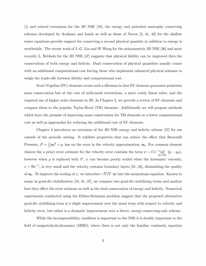
[1] and related extensions for the 2D NSE [19], the energy and potential enstrophy conserving

schemes developed by Arakawa and Lamb as well as those of Navon [2, 41, 42] for the shallow

water equations provide support for conserving a second physical quantity in addition to energy is

worthwhile. The recent work of J.-G. Liu and W.Wang for the axisymmetric 3D NSE [36] and most

recently L. Rebholz for the 3D NSE [47] suggests that physical fidelity can be improved thru the

conservation of both energy and helicity. Dual conservation of physical quantities usually comes

with an additional computational cost forcing those who implement enhanced physical schemes to

weigh the trade-offs between fidelity and computational cost.

Scott-Vogelius (SV) elements create such a dilemma in that SV elements guarantee pointwise

mass conservation but at the cost of mild-mesh restrictions, a more costly linear solve, and the

required use of higher order elements in 3D. In Chapter 2, we provide a review of SV elements and

compare them to the popular Taylor-Hood (TH) elements. Additionally we will propose methods

which have the promise of improving mass conservation for TH elements at a lower computational

cost as well as approaches for reducing the additional cost of SV elements.

Chapter 3 introduces an extension of the 3D NSE energy and helicity scheme [47] for use

outside of the periodic setting. It exhibits properties that can reduce the effect that Bernoulli

Pressure, P = 12 |u|

2 + p, has on the error in the velocity approximation, uh. For common element

choices the a priori error estimate for the velocity error contains the term ψ = Cν−1 infqh∈Qh

‖p− qh‖,

however when p is replaced with P , ψ can become poorly scaled when the kinematic viscosity,

ν = Re−1, is very small and the velocity contains boundary layers [21, 34], diminishing the quality

of uh. To improve the scaling of ψ, we introduce γ∇(∇·u) into the momentum equation. Known to

many as grad-div stabilization [10, 31, 37], we compare two grad-div stabilizing terms and analyze

how they effect the error estimate as well as the dual conservation of energy and helicity. Numerical

experiments conducted using the Ethier-Steinman problem suggest that the proposed alternative

grad-div stabilizing term is a slight improvement over the usual term with respect to velocity and

helicity error, but either is a dramatic improvement over a direct, energy-conserving-only scheme.

While the incompressibility condition is important to the NSE it is doubly important to the

field of magnetohydrodynamics (MHD), where there is not only the familiar continuity equation

2

for velocity, ∇ · u = 0, but also a solenoidal condition on the magnetic field, ∇ · B = 0. The

study of MHD pertains to the interaction of fluid flow and magnetic fields which are often used

to heat, pump, stir and levitate liquid metals in the metallurigical industries [11]. In order for

the interaction of the fluid and magnetic field to be substantial the fluids in question must be

conductors and non-magnetic, which includes liquid metals, plasmas and strong electrolytes. At

one time MHD was perhaps best known for its association with colossal failures in power generation

[11], however in the last 30 years MHD has been found to be pertinent to the flow of liquid sodium

coolants in fast-breeder reactors, and the confinement of hot plasma thru magnetic forces during

controlled thermonuclear fusion. Via the extension of the philosophy of enhanced physics, we were

able to develop a numerical scheme for MHD flows which possesses both dual-conservation, energy

and cross-helicity, and enforces pointwise incompressibility ‖∇ · uh‖ = ‖∇ ·Bh‖ = 0.

This thesis is arranged as follows. Chapter 2 provides an introduction to the Scott-Vogelius

elements and some preliminary comparisons of results against Taylor-Hood elements. Chapter 3

presents the extension of the energy-helicity conserving scheme to the case of wall-bounded flows.

In chapter 4, we study the SV elements for approximating solutions to the NSE, and establish an

important connection between these solutions and those found using Taylor-Hood elements and

grad-div stabilization. Chapter 5 derives and analyzes a new scheme for MHD flows that conserves

energy and cross-helicity globally, and enforces incompressibility of the magnetic and velocity fields

pointwise. A rigorous stability and convergence analysis of the scheme is presented.

3

Chapter 2

Scott-Vogelius Elements

Our interest in the Scott-Vogelius elements stems from the property, for (Xh, Qh) = (Pk, Pdisck−1 )

with k ≥ dim, and if the mesh is constructed as a barycenter refinement of a quasi-uniform mesh,

this element pair is LBB stable and satisfies

∇ ·Xh ⊂ QSVh . (2.1)

As a result of (2.1) when we consider the weak formulation of the incompressibility condition

(qh,∇ · uh) = 0,

we can select our test function, qh, such that

qh = ∇ · uh ⇒ ‖∇ · uh‖2 = 0.

In general, a naive selection for the discrete pressure space can introduce numerical insta-

bility into the approximation. More specifically if Qh is chosen too large in relation to the discrete

velocity space, such that if ΠQhL2 denotes the L2 projection operator into Qh, the discrete divergence

operator divh : Xh → Qh with divhvh := ΠQhL2 is not surjective and equivalently LBB is not satisfied.

The absence of LBB removes the usual stability condition on the pressure permitting erroneous

oscillations to appear which ultimately diminishes the quality of uh. The idea of using (Pk, Pdisck−1)

4

as an element pair is first attributed to [52], recent extensions of SV elements in [58, 34, 6] to Stokes

flow, Steady NSE equations and Oseen equations support our investigation into the merits of SV

element approximations for the time dependent incompressible NSE equations.

We note that Scott-Vogelius elements are implemented using a Clough-Tocher macro-

element to tessellate all of Ω. This is usually done by taking an existing quasi-uniform conforming

mesh and creating a Clough-Tocher macro-element out of each element in the tessellation. In prac-

tice we have not found this to be a considerable hurdle, while there does not appear to be any

commercial software which explicitly offers a barycentric refinement we feel that the majority of

scientists will be able to implement the mesh restriction fairly easily. The barycentric refinement

is necessary to ensure LBB holds [34, 58], in fact any refinement in which a 4-way split is achieved

will have the property of LBB stability, refining about the barycenter helps to ensure a balanced

mesh while also simplifying the proof given in [58].

Pointwise mass-conservation for the NSE has also been achieved with Discontinuous Galerkin

(DG) schemes such as those in [8, 9]. We note that these proposed DG schemes make the assumption

that u ∈ H(div) as opposed to H1(Ω) and often utilize a post processing routine to achieve point-

wise mass-conservation. Furthermore DG methods are often difficult to extend to existing legacy

codes for the NSE where as SV elements have the promise of obtaining pointwise mass conservation

without the headaches of extending existing routines to DG. Results for similar element pairs that

satisfy LBB and ∇ ·Xh ⊆ Qh are presented in [59, 60]. We feel SV elements are advantageous to

the element pairs proposed in [59, 60] as “serious” computing is going to be done with triangles and

tetrahedra opposed to quadrilaterals and parallelepipeds, while the Powell-Sabin splits proposed in

[60] enforce a stricter mesh restriction and have yet to be extended to three dimensions.

In the sequel, we will compare SV elements to TH elements. These elements differ in

structure only in that the pressure space for TH elements is continuous, although the TH element

has less restrictions in order to be LBB stable. Hence, on the same mesh, the Xh space is the same

for both elements, but Qh is not, and so will be labeled with superscripts to distinguish. Moreover,

the subspace of discretely divergence free functions in Xh, called Vh and defined by

Vh := vh ∈ Xh : (∇ · vh, qh) = 0 ∀qh ∈ Qh,

5

will also differ and be similarly labeled.

An unanticipated advantage to utilizing QSVh is competitive assembly despite the increase

in dim(Qh), which can be attributed to the lack of dependence SV elements have on neighboring

elements when the B block is assembled. Assembly can also be improved in the A block as

we can handle the nonlinearity more efficiently due to pointwise mass conservation. For high-level

computing assembly is usually deemed negligible with respect to computational cost when compared

with the cost of the linear solve. With the dim(QSVh ) > dim(QTHh ) SV elements require a significant

bump in computational cost on equivalent meshes. The extent of the additional cost in the linear

solve is being actively studied, however we do not think it is unreasonable for preconditioners

similar to those presented in [3, 39, 4, 13, 15] to reduce the additional cost as the A block is

identical for both SV and TH elements. In addition to computational cost there is also a concern

for the resulting velocity error as

dim(Vh) = dim(Xh)− dim(Qh).

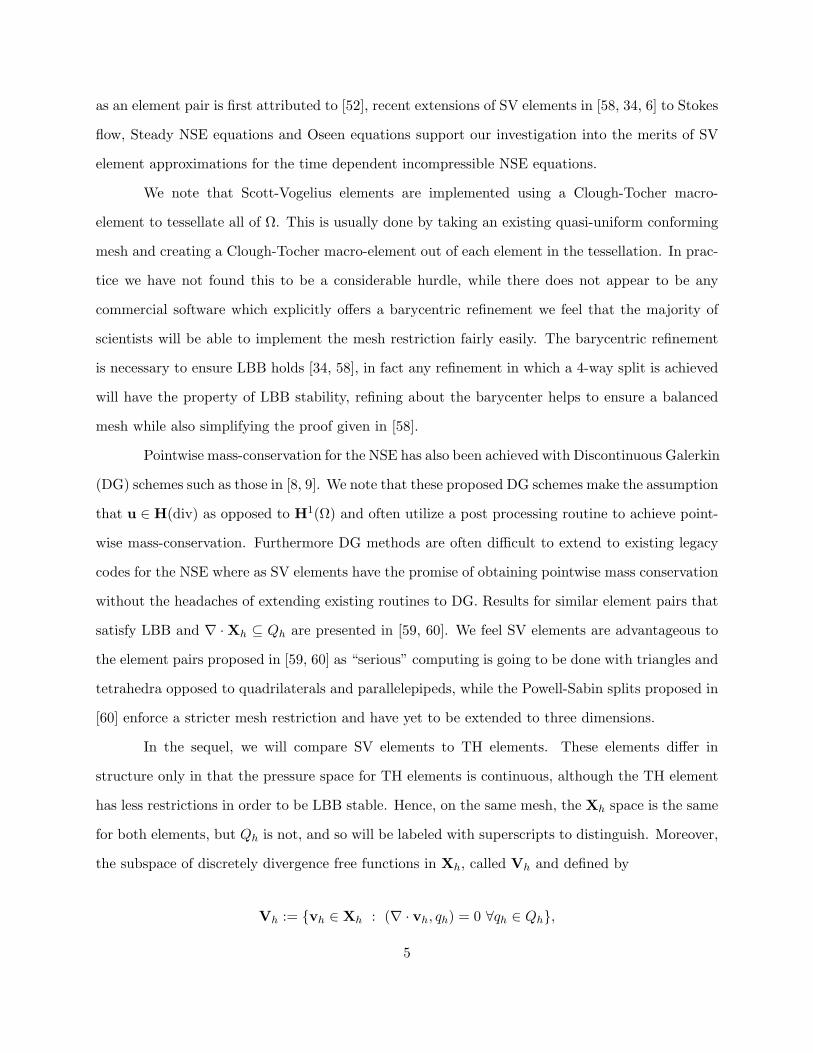
Figure 2.1: (LEFT) 2D and (RIGHT) 3D Clough-Tocher macro-element, shown with dashed linesrepresenting barycenter refinements

2.0.1 Preliminary numerical experiments

In the forthcoming numerical experiments for Stokes Flow and the time dependent incom-

pressible NSE we attempt to compare (Pk, Pk−1) elements with (Pk, Pdisck−1). When constructing

these experiments we wanted to highlight the advantages of SV elements and the low quality of

6

Figure 2.2: (LEFT) 2D conforming mesh and (RIGHT) mesh resulting from barycentric refinement.

the enforcement of mass conservation seen in TH element approximations. For the Stokes Flow

experiment we attempted to compare SV elements with TH elements when similar total dof are

used. The time-dependent examples for both two and three dimensional flow compare results for

the same mesh. Despite the advantage in the total dof since VSVh ⊂ VTH

h , SV elements are already

at a competitive disadvantage with respect to L2 error on the same mesh. With that said, one

should not come away from the forthcoming comparisons with the impression TH elements are

incapable of resolving the velocity field for a comparable total dof.

2.0.1.1 Stokes Flow

We first consider the Stokes Equations on Ω = (−1, 1)3:

− ν∆u +∇p = f , (2.2)

∇ · u = 0. (2.3)

7

We can form a finite element scheme for the solution of the Stokes problem:

find (uh, ph) ∈ (Xh, Qh) s.t. (2.4)

ν(∇uh,∇vh)− (∇ · vh, ph) = f , ∀vh ∈ Xh, (2.5)

(∇ · uh, qh) = 0, ∀qh ∈ Qh. (2.6)

Choosing u = [cos(Nπz), sin(Nπz), sin(Nπx)] and p = cos(Nπ(x+y)) gives us a nontrivial

Stokes problem and helps us illustrate how poor mass conservation can be when using Taylor-Hood

elements.

Table 2.1: Sample Problem Velocity Error, ν = 1.0..

Elem. N dim(Vh) L2 Error H1 Error ‖div uh‖TH32 2 31620 0.0058 0.1914 0.1549SV32 2 8511 3.89e-4 0.0071 5.151e-14TH32 8 31620 0.0678 1.4555 0.4165SV32 8 8511 0.1021 2.029 4.795e-14

The results from Table 2.1 suggest that Taylor-Hood elements can have respectable velocity

error for a simple flow while doing a poor job of conserving mass. For the N = 2 case, the Scott-

Vogelius solution has better L2 and H1 velocity errors. However, for N = 8, Taylor-Hood solutions

have slightly better errors. Although not shown, from the table the H(div) norm can be calculated,

and the Scott-Vogelius solution would be better in this norm for N = 8.

We now consider the Stokes problem with pressure stabilization

∇pε − ν∆uε = f , on Ω, (2.7)

div uε + εpε = 0 on Ω. (2.8)

(2.9)

8

which has the following weak formulation,

find (uh, ph) ∈ (Xh, Qh) s.t.

−(pε,∇ · qh) + ν(∇uε,vh) = f , ∀vh ∈ Xh, (2.10)

div uε + εpε = 0,∀qh ∈ Qh. (2.11)

Table 2.2: Sample Problem Velocity Error, ν = 1.0. w/Pres. Stab., ε = 1.0e-6.

Elem. N dim(Vh) L2 Error H1 Error ‖div uh‖TH32 2 31620 0.0058 0.1914 0.1549SV32 2 8511 3.890e-4 0.0071 2.1391e-6TH32 8 31620 0.0678 1.4539 0.4165SV32 8 8511 0.1022 2.0298 1.971e-6

The Stokes results in Tables 2.1 & 2.2 were computed for (P3, Pdisc2 ) elements on a 4×4×4

mesh with barycenter refinement resulting in 39,231 total dof, 23,871 velocity dof and 15,360

pressure dof. (P3, P2) results were generated on a 6×4×4 mesh with barycenter refinement giving

us 39,486 total dof, 23,871 vel. dof and only 3,933 pres. dof. These results suggest that Scott-

Vogelius elements drastically improve mass-conservation for similar computational cost, while also

improving the conditioning of the linear system in the presence of pressure stabilization. Pressure

stabilization does require additional assembly and storage of another matrix block but relative to

the assembly of the A block the extra work is not significant. Additionally pressure stabilization

allows us to drop the condition on the pressure nodes (i.e. Dirichlet,∫p dx = 0). The results

for Stokes Flow further support the concept that we cannot expect Scott-Vogelius elements to

provide an improvement in error in the L2 or H1 norms, even when the total dof are comparable

as dim(VhSV ) < dim(Vh

TH). However, we can expect improvement in error in the H(div) norm.

9

2.0.2 Time Dependent NSE results

For time dependent flow we use the following Crank-Nicholson Galerkin temporal-spatial

discretization,

find (uh, ph) ∈ (Xh, Qh),

(u0h,vh) + (λ,∇ · vh) + (∇ · u0

h, qh) = (u0,vh), ∀vh ∈ Vh, (2.12)

1∆t

(un+1h − unh,vh)− (p

n+ 12

h ,∇ · vh) + ν(∇un+ 1

2h ,∇vh)

+(un+ 1

2h · ∇u

n+ 12

h ,vh)+12

((∇ · un+ 12

h )un+ 1

2h ,vh) = (fn+ 1

2 ,vh), ∀vh ∈ Xh, (2.13)

(qh,∇un+ 1

2h ) = 0, ∀qh ∈ Qh, (2.14)

where n = 1, 2, . . . ,M = T/∆t.

2.0.2.1 Time Dependent Flow around a cylinder

2D flow around a cylinder is a well studied benchmark problem [29, 31, 27, 50]. In this

experiment Ω is defined by (0, 2.2)× (0, 0.41) representing a thin channel with flow in the positive x

direction with a circle of radius 0.05 centered at (0.2, 0.2). No-slip boundary conditions are applied

on the top and bottom of the channel along with the boundary of the cylinder.

The time dependent inflow and outflow profiles are enforced on the left and right boundaries:

u(0, y, t) = u(2, 2, y, t) =6

0.412[sin(πt/8)y(0.41− y), 0], 0 ≤ y ≤ 0.41. (2.15)

The forcing is set to zero, f = 0 and the viscosity, ν = 0.001 proving a time dependent

Reynolds number, 0 ≤ Re(t) ≤ 100. The initial condition is u0 = 0, while we approximate up to

T = 8 with a time step of ∆t = 0.01.

An accurate prediction of the velocity field will predict a vortex street forming behind the

cylinder at t = 4 and a fully formed vortex street by t = 7. We note that in addition to the velocity

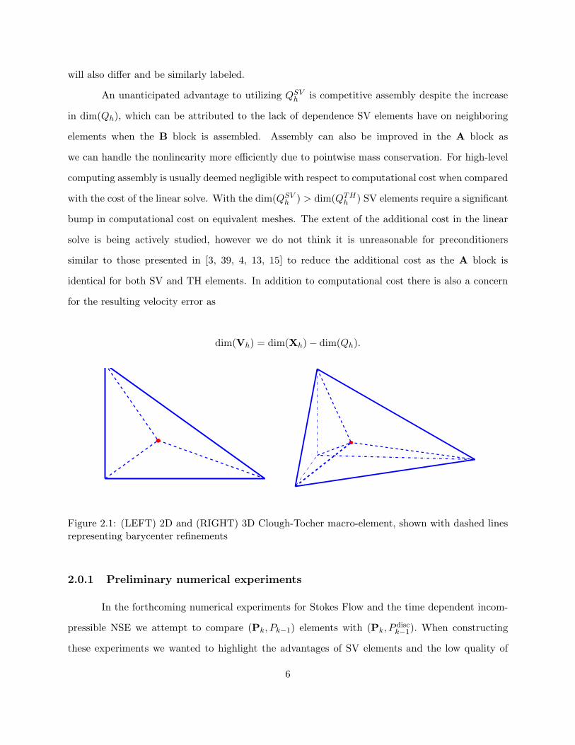
field we will be measuring the quality of div uh. We compared Scott-Vogelius and Taylor-Hood

elements using the mesh depicted in Figure 2.3 resulting in 6,578 velocity dof for each element type

10

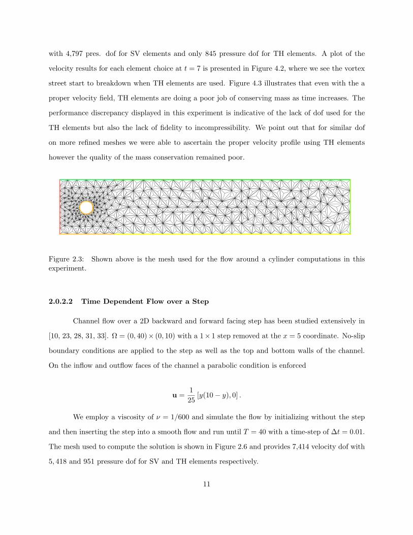
with 4,797 pres. dof for SV elements and only 845 pressure dof for TH elements. A plot of the

velocity results for each element choice at t = 7 is presented in Figure 4.2, where we see the vortex

street start to breakdown when TH elements are used. Figure 4.3 illustrates that even with the a

proper velocity field, TH elements are doing a poor job of conserving mass as time increases. The

performance discrepancy displayed in this experiment is indicative of the lack of dof used for the

TH elements but also the lack of fidelity to incompressibility. We point out that for similar dof

on more refined meshes we were able to ascertain the proper velocity profile using TH elements

however the quality of the mass conservation remained poor.

Figure 2.3: Shown above is the mesh used for the flow around a cylinder computations in thisexperiment.

2.0.2.2 Time Dependent Flow over a Step

Channel flow over a 2D backward and forward facing step has been studied extensively in

[10, 23, 28, 31, 33]. Ω = (0, 40)× (0, 10) with a 1× 1 step removed at the x = 5 coordinate. No-slip

boundary conditions are applied to the step as well as the top and bottom walls of the channel.

On the inflow and outflow faces of the channel a parabolic condition is enforced

u =125

[y(10− y), 0] .

We employ a viscosity of ν = 1/600 and simulate the flow by initializing without the step

and then inserting the step into a smooth flow and run until T = 40 with a time-step of ∆t = 0.01.

The mesh used to compute the solution is shown in Figure 2.6 and provides 7,414 velocity dof with

5, 418 and 951 pressure dof for SV and TH elements respectively.

11

Velocity field streamlines with speed contours are shown at T = 10, 20, 30 and 40 for the

SV element solution in Figure 2.7 and for TH elements in Figure 2.8. The SV element solution

forms and sheds eddies, has a smooth velocity profile, and in general agrees with the “true” solution

found in [32], which utilizes 27,228 total dof. The TH element solution is observed to be slightly

underresolved. Although it forms and sheds eddies, by T = 40, the eddies behind the step appear

to be stretching instead of detaching. Moreover, the velocity field is developing oscillations evident

in the speed contours. Figure 2.9 displays a poor quality of mass conservation for TH elements

comparable to what we have observed in the previous experiments.

2.0.2.3 3D Lid -Driven Cavity

The Lid-driven cavity problem is a popular benchmark problem described in greater detail

within [57, 44]. Ω = (−1, 1)3 with no-slip boundary conditions applied to all of the walls except on

the boundary where z = 1, the lid. The lid has a profile of [1, 0, 0] which is imposed on u at the

boundary. Viscosity at ν = 1/50, yields a Reynolds number, Re = 2 · 50 = 100 while we impose

that u0 = 0. The mesh for this experiment is displayed in Figure 2.10 and has 57,804 velocity

dof with 6,360 pressure dof for TH elements and 37,840 pressure dof for SV type. The problem

is solved directly for the steady solution with a Newton iteration taking 7 iterations to converge

to a tolerance of 10−10 for each element type. Figures 2.11 and 2.12 display vector fields which

closely resemble those in [57, 44] while Figure 2.13 supports a near-accurate flow for both elements.

However, as we have seen in the previous experiments the mass conservation for TH elements,

depicted in Figure 2.12, is poor especially in the corners for each midplane.

2.0.3 Discussion of Results

The numerical results appear to support the use of SV elements because of their ability

to provide pointwise mass conservation. However, TH elements were underresolved in some of

the experiments and not incapable of resolving the velocity field on fine meshes for comparable

computational cost, still the concern with implementing TH elements comes from the low quality

in mass conservation even when the velocity field appears to be correct as we saw in the driven cavity

12

experiment, thus how can any uh approximation be expected to have any physical meaning when

the quality of mass conservation is so poor. Furthermore, we feel these experiments support the

philosophy of enhanced physics as early on TH elements perform at a reasonable level with respect

to the velocity profiles for both the 2D cylinder and 2D step problem but ultimately breakdown as

time increases despite the fact that dim(VTHh ) > dim(VSV

h ).

We feel there is promise in extending the preliminary convective SV results given in this

section to not only rotational NSE schemes but any FEM scheme which enforces incompressibility.

Additionally we are interested in comparing the mass conservation results obtained thru

SV elements with those obtained for TH elements with grad-div stabilization in the momentum

equation on a barycenter-refined mesh. If a relationship between these basis functions can be

established it could aid greatly in reducing the computational cost of improved mass conservation

for NSE computations.

Finally we mention that we are interested in expanding on the physical problems presented

in this section (i.e. channel flow and two faced step problems). The current computer codes being

used to generate the results given in this report will be extended to parallel routines that will

allow for us to test our analytical results in a more efficient fashion and comment on existing

preconditioners for the NSE and their ability to offset the computational costs associated with SV

elements.

13

Velocity Field

Speed Countours

Pressure Contours

Velocity Field

Speed Contours

Pressure Contours

Figure 2.4: Shown above are the t=7 velocity fields, speed contours, and pressure contours plotsfor solution obtained using Scott-Vogelius elements (top) Taylor-Hood elements (bottom).

14

0 1 2 3 4 5 6 7 8

1e−13

0.5

1

1.5

2

2.5

3

time

|| d

iv u

h||

Cylinder problem, ν=1/1000

Scott−VogeliusTaylor−Hood

Figure 2.5: Shown above are the plots of ‖∇ · unh‖ vs. time for the SV and TH solutions for the2D cylinder problem.

Figure 2.6: The barycenter-refined mesh used for the 2D step computations

15

0 5 10 15 20 25 30 35 400

2

4

6

8

10

0 5 10 15 20 25 30 35 400

2

4

6

8

10

0 5 10 15 20 25 30 35 400

2

4

6

8

10

0 5 10 15 20 25 30 35 400

2

4

6

8

10

T = 40T = 30

T = 10 T = 20

Figure 2.7: For SV elements the flow profile appears to agree with the “true” solution[32].

16

0 5 10 15 20 25 30 35 400

2

4

6

8

10

0 5 10 15 20 25 30 35 400

2

4

6

8

10

0 5 10 15 20 25 30 35 400

2

4

6

8

10

0 5 10 15 20 25 30 35 400

2

4

6

8

10

T = 10 T = 20

T = 40T = 30

Figure 2.8: For TH elements the velocity field is underresolved and fails to shed eddies at T = 40.

17

0 5 10 15 20 25 30 35 40

1e−13

0.2

0.4

0.6

0.8

1

1.2

1.4

time

|| d

iv u

h||

Step problem, ν=1/600

Scott−VogeliusTaylor−Hood

Figure 2.9: Shown above are the plots of ‖∇ · unh‖ vs. time for the SV and TH solutions for the 2Dstep problem.

18

Figure 2.10: The barycenter-refined mesh used for the 3D lid-driven cavity problem.

x

y

x

z

Midplane Velocity Fields and Divergence Contours for Scott!Vogelius Element Solution

y

z

x

y

!6 !4 !2 0 2x 10!15

x

z

!5 0 5 10x 10!14

y

z

!2 0 2x 10!14

Figure 2.11: 3D lid-driven cavity results with SV elements. Note the small scale next to the colorbar.

19

xy

x

z

Midplane Velocity Fields and Divergence Contours for Taylor!Hood Element Solution

y

z

x

y

!0.05 0 0.05

x

z

!2 !1.5 !1 !0.5 0 0.5

y

z

!0.5 0 0.5

Figure 2.12: 3D lid-driven cavity results with TH elements. Note the scale next to the color barand the contours in the corners of each midplane.

0 0.1 0.2 0.3 0.4 0.5 0.6 0.7 0.8 0.9 1!0.4

!0.2

0

0.2

0.4

0.6

0.8

1Centerline x velocity for Re=100 driven cavity steady state

z

u1(0

.5,0

.5,z

)

Wong/Baker, 705,894 dofTH32 64,164 dofSV32 95,644 dof

Figure 2.13: 3D lid-driven cavity results compared to “true” solution on centerline.

20

Chapter 3

Stable computing with an enhanced

physics based scheme for the 3d

Navier-Stokes equations

3.1 Introduction

This chapter extends the methodology of the enhanced-physics based scheme for the 3D

Navier-Stokes equations (NSE) proposed in [47] (defined in Section 2) from its original derivation

for space-periodic problems to a more general class of problems. This scheme is referred to as

enhanced-physics because it is the only scheme that conserves both discrete energy and discrete

helicity for the full 3D NSE. The key ingredient for the dual conservation scheme is using the

rotational form of the nonlinearity with a projected vorticity, which allows the discrete nonlinearity

to preserve both of the quantities. Since the (continuous) NSE nonlinearity conserves both energy

and helicity, and jointly cascades them from the large scales through the inertial range to small

viscosity dominated scales [7, 12], if the discrete nonlinearity does not also conserve energy and

helicity it will introduce numerical error into the cascade, and bring into question the physical

relevance of computed approximations.

It is a widely held belief in computational fluid dynamics (CFD) that the more physically

21

correct a numerical scheme is, the more accurate its predictions will be, especially over long time

intervals. In systems of conservation laws for fluids there is typically a second integral invariant

in addition to energy, and its accurate treatment in a numerical scheme generally produces more

accurate simulations than do schemes that do not specifically conserve this quantity. Beginning

with Arakawa’s energy and enstrophy conserving scheme for the 2D NSE [1] and related extensions

[19], to energy and potential enstrophy schemes pioneered by Arakawa and Lamb, and Navon,

[2, 41, 42], and most recently to an energy and helicity conserving scheme for 3D axisymmetric

flow by J.-G. Liu and W. Wang [36], enhanced physics based schemes have provided more accurate

simulations, especially over longer time intervals.

The fundamental challenge in extending the scheme of [47] to non-periodic problems is to

avoid the large errors often present when the rotational form of the nonlinearity and the Bernoulli

pressure is used. In the usual a priori error analysis for the velocity approximation for the NSE, a

consequence that the discrete divergence free velocity is not exactly divergence free, is a pressure

error contributionC

νinf

qh∈Qh‖p− qh‖ , (3.1)

where ν = 1/Reynolds number denotes the kinematic viscosity [21, 34]. For problems whose

pressure gradients are small this term is often negligible. However, using the rotational form of the

NSE, and introducing the Bernoulli pressure p+ 12 |u|

2 can bring prominence to this term, since the

gradient of the Bernoulli pressure may be large due to boundary layers in the velocity field.

Following recent work in [31, 37, 10], a natural way to mitigate the pressure’s error influence

on the velocity approximation is to introduce grad-div stabilization. As we show, this reduces the

effect of the Bernoulli pressure error. In the interest of physical fidelity, we also introduce a

modified grad-div stabilization having the same effect on the error, but with less impact on the

energy balance. Computational results show a slight improvement when this alternate stabilization

is used instead of usual grad-div stabilization.

This chapter is arranged as follows. Section 2 presents mathematical preliminaries and

notation, and defines the scheme studied in the remainder of the chapter. Section 3 is a study

of stability and conservation laws for the scheme, and Section 4 presents a rigorous convergence

22

analysis. Section 5 shows a numerical example which clearly illustrates the advantage of the scheme.

Concluding remarks are given in Section 6.

3.2 Mathematical Preliminaries

We assume that Ω denotes a polyhedral domain in R3. The L2(Ω) norm and inner product

are denoted by ‖·‖ and (·, ·). Likewise, the Lp(Ω) norms and the Sobolev W kp (Ω) norms are denoted

‖ · ‖Lp and ‖ · ‖Wkp

, respectively. For the semi-norm in W kp (Ω) we use | · |Wk

p. Hk is used to represent

the Sobolev space W k2 (Ω), and ‖ · ‖k denotes the norm in Hk. For functions v(x, t) defined on the

entire time interval [0, T ], we define (1 ≤ m <∞)

‖v‖∞,k := ess sup[0,T ]‖v(t, ·)‖k , and ‖v‖m,k :=

(∫ T

0‖v(t, ·)‖mk dt

)1/m

.

For the analysis, we assume no slip (i.e. homogeneous Dirichlet) boundary conditions for

velocity and therefore use as our velocity and pressure spaces

X := (H10 (Ω))d, Q := L2

0(Ω) ,

where Q is denoting the mean zero subspace of L2(Ω).

We use as the norm on X the H1 seminorm which, because of the boundary condition, is a

norm, i.e. for v ∈ X, ‖v‖X := ‖∇v‖. We denote the dual space of X by X?, with the norm ‖ · ‖?.

The space of divergence free functions is defined by

V := v ∈ X : (∇ · v, q) = 0 ∀q ∈ Q .

We denote conforming velocity, pressure finite element spaces based on a regular tetrahe-

dralization, Th, of Ω (with maximum tetrahedron diameter h) by

Xh ⊂ X, Qh ⊂ Q.

23

We assume that Xh, Qh satisfy the usual inf-sup condition necessary for the stability of the pressure,

i.e.

infqh∈Qh

supvh∈Xh

(qh,∇ · vh)‖qh‖ ‖vh‖X

. (3.2)

Specifically, we assume that (Xh, Qh) is made of (Pk, Pk−1), k ≥ 2 velocity pressure elements. Thus

we have, for a given regular tetrahedralization Th,

Xh :=vh : vh|e ∈ Pk(e), ∀e∈Th , vh ∈ [C0(Ω)]3, vh|∂Ω = 0

,

Qh :=qh : qh|e ∈ Pk−1(e), ∀e∈Th , qh ∈ C

0(Ω), qh ∈ L20(Ω)

.

The discretely divergence free subspace of Xh is

Vh = vh ∈ Xh : (∇ · vh, qh) = 0 ∀qh ∈ Qh .

We also use a more general space for the discrete vorticity space. Even though the velocity

satisfies homogeneous Dirichlet boundary conditions, it is believed to be inappropriate to enforce

homogeneous Dirichlet boundary conditions for the vorticity. A more physically consistent bound-

ary condition is instead a no-slip boundary condition along the boundary, and hence we define the

space

Wh :=vh : vh ∈ [C0(Ω)]3, ∀e∈Th(vh)|e ∈ Pk(e), vh × n|∂Ω = 0

⊃ Xh .

We use tn := n∆t, and for both continuous and discrete functions of time

vn+ 12 :=

v((n+ 1)∆t) + v(n∆t)2

.

3.2.1 Enhanced-physics based numerical schemes

We study three variations of the enhanced-physics based scheme of [47] extended to homo-

geneous Dirichlet boundary conditions for velocity. The first is a direct extension of the scheme

to homogeneous boundary conditions. The second scheme adds usual grad-div stabilization (see

[46]), that is, it adds the term γ(∇ · (un+1h + unh)/2,∇ · vh) to a Crank-Nicolson scheme. This term

24

is derived from adding the (identically zero) term −γ∇(∇ · u) at the continuous level. Discretely,

this term penalizes for lack of mass conservation, and is known to reduce the effect of the pressure

error on the velocity error for large Reynolds number problems [31, 37, 46]. In finite element com-

putations of rotational form models the (Bernoulli) pressure error tends to be the dominant error

source because it is as complex as the velocity but is approximated with lower degree polynomials,

and its effect on the velocity error is amplified by the Reynolds number. The potential downside

from using this stabilization is a change in the energy balance. However, in practice this tradeoff

is worthwhile.

In the interest of physical fidelity to the energy balance, in the third scheme we introduce an

alternative stabilization that provides the same effect on reducing the effect of the pressure error on

the velocity error, but with minimal impact on the physical energy balance (Section 3). The added

stabilization term arises by adding the (also identically zero) term −γ∇(∇ · ut) at the continuous

level, leading to the term γ 1∆t(∇ · (u

n+1h − unh),∇ · vh) in the FEM formulation. The computational

results (Section 5) from using this stabilization show an improvement in accuracy over the usual

grad-div stabilization for our test problem. However, we note that for steady problems this term

will not have a stabilizing effect since it will be trivially zero.

There has been recent work done to optimally choose the constant γ that scales the stabi-

lization term. Herein, we simply choose γ = 1 in the computations, which the analysis suggests is

an appropriate choice. However, one could also choose this parameter element-wise, which would

lead to better results [43]. We leave optimal parameter choice for these schemes as an interesting

topic of future study.

Algorithm 3.2.1 (Enhanced-physics based schemes for homogeneous Dirichlet boundary condi-

tions). Given a time step ∆t > 0, finite end time T := M∆t, and initial velocity u0h ∈ Vh, find

w0h ∈Wh and λ0

h ∈ Qh satisfying ∀(χh, rh) ∈ (Wh, Qh)

(w0h, χh) + (λ0

h,∇ · χh) = (∇× u0h, χh), (3.3)

(∇ · w0h, rh) = 0. (3.4)

25

Then for n = 0, 2, ...,M − 1, find (un+1h , wn+1

h , pn+1h , λn+1

h ) ∈ (Xh,Wh, Qh, Qh) satisfying

∀(vh, χh, qh, rh) ∈ (Xh,Wh, Qh, Qh)

(un+1h − unh

∆t, vh) + STAB− (pn+1

h ,∇ · vh)

+(wn+ 1

2h × un+ 1

2h , vh) + ν(∇un+ 1

2h ,∇vh) = (f(tn+ 1

2 ), vh) (3.5)

(∇ · un+1h , qh) = 0 (3.6)

(wn+ 1

2h , χh) + (λn+1

h ,∇ · χh) = (∇× un+ 12

h , χh) (3.7)

(∇ · wn+ 12

h , rh) = 0. (3.8)

where

STAB =

0 Scheme 1

γ(∇ · un+ 12

h ,∇ · vh) Scheme 2

γ∆t(∇ · (u

n+1h − unh),∇ · vh) Scheme 3

Remark 1. We have found it computationally advantageous to decouple the 4 equation system

(3.5)-(3.8) into a velocity-pressure system (3.5)-(3.6) and a projection system (3.7)-(3.8), then

solve (3.5)-(3.8) by iterating between the two sub-systems. This typically requires more iterations

and linear solves to converge than solving the fully-coupled system using a Newton method. However

the linear solves are much easier in the decoupled system. Note also that for the decoupled system

the work required is only slightly more than a usual implicit Crank-Nicolson method (i.e. without

vorticity projection) since the extra work is (relatively inexpensive) projection solves. Moreover, for

nonhomogeneous boundary conditions, this decoupling leads to a simplified boundary condition for

the vorticity: wh = Ih(∇× uh) on the boundary, where Ih is an appropriate interpolation operator.

3.3 Stability, conservation laws, and existence of solutions

In this section we prove fundamental mathematical and physical properties of the 3 schemes:

unconditional stability, solution existence and conservation laws. We begin with stability.

Lemma 3.3.1. Solutions to Algorithm 3.2.1 are nonlinearly stable. That is, they satisfy:

26

Scheme 1: ∥∥uMh ∥∥2+ ν∆t

M−1∑n=0

∥∥∥∥∇un+ 12

h

∥∥∥∥2

≤ ∆tν

M−1∑n=0

‖f‖2∗ +∥∥u0

h

∥∥2 = C(data) . (3.9)

Scheme 2:

∥∥uMh ∥∥2+ ∆t

M−1∑n=0

(2γ∥∥∥∥∇ · un+ 1

2h

∥∥∥∥2

+ ν

∥∥∥∥∇un+ 12

h

∥∥∥∥2)≤ ∆t

ν

M−1∑n=0

‖f‖2∗ +∥∥u0

h

∥∥2 = C(data) . (3.10)

Scheme 3:

∥∥uMh ∥∥2+ γ

∥∥∇ · uMh ∥∥2+ ν∆t

M−1∑n=0

∥∥∥∥∇un+ 12

h

∥∥∥∥2

≤ ∆tν

M−1∑n=0

‖f‖2∗ +∥∥u0

h

∥∥2 + γ∥∥∇ · u0

h

∥∥ = C(data) . (3.11)

Schemes 1,2,3:

∆tM−1∑n=0

∥∥∥∥wn+ 12

h

∥∥∥∥2

≤ ∆tM−1∑n=0

∥∥∥∥∇un+ 12

h

∥∥∥∥2

= C(data) . (3.12)

Schemes 1,2,3:

∆tM∑n=1

(‖pnh‖

2 + ‖λnh‖2)≤ C(data) . (3.13)

C(data) is a constant dependent on T, ν, γ, f, u0h and Ω.

Proof. To prove the bounds on velocity for each of the schemes, choose vh = un+ 1

2h in (3.5). The

nonlinear and pressure terms are then zero. The triangle inequality, and summing over time steps

then completes the proofs of (3.9),(3.10),(3.11).

To prove (3.12) choose χh = wn+ 1

2h in (3.7) and rh = λn+1

h in (3.8). After combining the

equations we obtain

∥∥∥∥wn+ 12

h

∥∥∥∥2

= (∇× un+ 12

h , wn+ 1

2h ) ≤

∥∥∥∥∇× un+ 12

h

∥∥∥∥∥∥∥∥wn+ 12

h

∥∥∥∥≤ 1

2

∥∥∥∥∇× un+ 12

h

∥∥∥∥2

+12

∥∥∥∥wn+ 12

h

∥∥∥∥2

≤∥∥∥∥∇un+ 1

2h

∥∥∥∥2

+12

∥∥∥∥wn+ 12

h

∥∥∥∥2

.

Rearranging, and summing over time steps we obtain (3.12).

27

To obtain the stated bound for λnh, we begin with the inf-sup condition satisfied by Xh (⊂

Wh) and Qh and use (3.7) to obtain

‖λnh‖ ≤1β

supχh∈Xh

(λnh,∇ · χh)‖χh‖X

≤ 1β

supχh∈Xh

(∇× un−12

h , χh)− (wn− 1

2h , χh)

‖χh‖X

≤ 1β

(‖∇ × un−

12

h ‖+ ‖wn−12

h ‖)≤ 2β

(‖∇un−

12

h ‖+ ‖wn−12

h ‖).

Using the bounds for ∇un+ 12

h (see (3.9)-(3.11)) and wn+ 1

2h (see (3.12)) we obtain the bound for λnh.

The bound for the pressure is established in an analogous manner.

Lemma 3.3.2. Solutions exist to each of the three schemes presented in Algorithm 3.2.1.

Proof. For each of the schemes, this is a straight-forward extension of the existence proof given for

the periodic case in [47]. The result is a consequence of the Leray-Schauder fixed point theorem,

and the stability bounds of Lemma 3.3.1.

We now study the conservation laws for energy and helicity in the schemes. It is shown

in [47] that, when restricted to the periodic case, the non-stabilized scheme of Algorithm 3.2.1

(Scheme 1) conserves energy and helicity. In the case of homogeneous boundary conditions for

velocity, this physically important feature for energy is still preserved. However, as one might

expect, the stabilization terms in Schemes 2 and 3 alter the energy balance. Lemma 3.3.3 shows

these energy balances.

The energy balance of Scheme 1, the unstabilized scheme, is analogous to that for the

continuous NSE. However, for Scheme 2, we see the effect of the stabilization on the energy balance

in the term γ∆t∑M−1

n=0

∥∥∥∥∇ · un+ 12

h

∥∥∥∥2

on the left hand side of (3.15). For most choices of elements,

one may have that each term in this sum is small, but over a long time interval this sum can grow

to significantly (and non-physically) alter the balance. The energy balance for Scheme 3 differs

from Scheme 1’s energy balance in the addition of only two small terms, instead of a sum. Hence

this indicates that the modified grad-div stabilization, for problems over a long time interval, offers

a more physically relevant energy balance than the usual grad-div stabilization (Scheme 2).

28

Lemma 3.3.3. The schemes of Algorithm 3.2.1 admit the following energy conservation laws.

Scheme 1:

12

∥∥uMh ∥∥2+ ν∆t

M−1∑n=0

∥∥∥∥∇un+ 12

h

∥∥∥∥2

= ∆tM−1∑n=0

(f(tn+ 12 ), u

n+ 12

h ) +12

∥∥u0h

∥∥2. (3.14)

Scheme 2:

12

∥∥uMh ∥∥2+ ν∆t

M−1∑n=0

∥∥∥∥∇un+ 12

h

∥∥∥∥2

+ γ∆tM−1∑n=0

∥∥∥∥∇ · un+ 12

h

∥∥∥∥2

= ∆tM−1∑n=0

(f(tn+ 12 ), u

n+ 12

h ) +12

∥∥u0h

∥∥2.

(3.15)

Scheme 3:

12

(∥∥uMh ∥∥2

+ γ∥∥∇ · uMh ∥∥2

) + ν∆tM−1∑n=0

∥∥∥∥∇un+ 12

h

∥∥∥∥2

= ∆tM−1∑n=0

(f(tn+ 12 ), u

n+ 12

h )

+12

(∥∥u0

h

∥∥2 + γ∥∥∇ · u0

h

∥∥2) . (3.16)

Proof. The proofs of these results follow from choosing vh = un+ 1

2h in Algorithm 3.2.1 for each of

the schemes. The key point is that the nonlinear term vanishes with this choice of test function,

and thus does not contribute to the energy balance equations.

We now consider the discrete helicity conservation in Algorithm 3.2.1. We begin with the

case of imposing Dirichlet boundary conditions on the projected vorticity, i.e. Wh = Xh. Although

this case is nonphysical, analysis of it is the first step in understanding more complex boundary

conditions.

In this case, the schemes’ discrete nonlinearity preserves helicity, however the stabilization

terms do not. We state the precise results in the next lemma. Denote the discrete helicity at time

level n by Hnh := (unh,∇× unh). Note that from (3.6),(3.7), Hn

h := (unh, wnh).

Lemma 3.3.4. If Wh := Xh, the schemes of Algorithm 3.2.1 admit the following helicity conser-

29

vation laws.

Scheme 1:

HMh + 2ν∆t

M−1∑n=0

(∇un+ 12

h ,∇wn+ 12

h ) = 2ν∆tM−1∑n=0

(f(tn+ 12 ),∇wn+ 1

2h ) +H0

h . (3.17)

Scheme 2:

HMh + 2ν∆t

M−1∑n=0

(∇un+ 12

h ,∇wn+ 12

h ) + 2γ∆tM−1∑n=0

(∇ · un+ 12

h ,∇ · wn+ 12

h )

= 2∆tM−1∑n=0

(f(tn+ 12 ),∇wn+ 1

2h ) +H0

h . (3.18)

Scheme 3:

HMh + 2ν∆t

M−1∑n=0

(∇un+ 12

h ,∇wn+ 12

h ) + 2γM−1∑n=0

(∇ · (un+1h − unh),∇ · wn+ 1

2h )

= 2∆tM−1∑n=0

(f(tn+ 12 ),∇wn+ 1

2h ) +H0

h . (3.19)

Proof. Choosing vh = wn+ 1

2h elimates the nonlinear term and the pressure term from (3.5) for each

of the 3 schemes, and reduces the time difference term to

1∆t

(un+1h − unh, w

n+ 12

h ) =1

∆t(un+1h − unh,∇× u

n+ 12

h )

=1

2∆t((un+1h ,∇× un+1

h ) + (un+1h ,∇× unh) − (unh,∇× un+1

h ) − (unh,∇× unh))

=1

2∆t(Hn+1h −Hn

h

), (3.20)

as, for v, w ∈ H10 (Ω), (v,∇× w) = (w,∇× v).

30

Using (3.20) Scheme 1 becomes,

12∆t

(Hn+1h −Hn

h

)+ ν(∇un+ 1

2h ,∇wn+ 1

2h ) = (f(tn+ 1

2 ), wn+ 1

2h ) (3.21)

Multiplying by 2∆t and summing over time steps completes the proof of (3.17).

The proofs of (3.18) and (3.19) follow the same way, except they will contain their respective

stabilization terms.

Lemma 3.3.4 shows that if we impose Dirichlet boundary conditions on the vorticity, then

the nonlinearity is able to preserve helicity. Hence for Scheme 1, we see a helicity balance analogous

to that of the true physics. However, the stabilization terms do not preserve helicity, and thus

appear in the helicity balances for Schemes 2 and 3.

Interestingly, if the term γ(∇ · wn+1h ,∇ · χh) is added to the left hand side of the vorticity

projection equation (3.7), one can show that Scheme 3 conserves both helicity and energy. This

results from the cancellation of the stabilization term in Scheme 3’s momentum equation when vh

is chosen to be wn+ 1

2h and χh is chosen as un+1

h and unh respectively. However, computations using

this additional term with Scheme 3 were inferior to those of Scheme 3 defined above.

Similar conservation laws for helicity, even for Scheme 1, do not appear to hold for the

nonhomogeneous boundary condition for vorticity, i.e. Xh 6= Wh. Due to the definitions of these

spaces, extra terms arise in the balance that correspond to the difference between the projection of

the curl into discretely divergence-free subspaces of Wh and Xh. These extra terms will be small

except at strips along the boundary, but nonetheless global helicity conservation will fail to hold.

However, more typical schemes, e.g. usual trapezoidal convective form or rotational form [30],

introduce nonphysical helicity over the entire domain and thus the schemes of Algorithm 2.1 still

provide a better treatment of helicity than such schemes.

3.4 Convergence

Three numerical schemes are described in Algorithm 2.1. We prove in detail convergence

of solutions of Scheme 3 to an NSE solution. Convergence results for Schemes 1 and 2 can be

31

established in an analogous manner.

We define the following additional norms:

‖|v|‖∞,k := max0≤n≤M

‖vn‖k , ‖|v1/2|‖∞,k := max1≤n≤M

‖vn−1/2‖k ,

‖|v|‖m,k :=

(M∑n=0

‖vn‖mk ∆t

)1/m

, ‖|v1/2|‖m,k :=

(M∑n=1

‖vn−1/2‖mk ∆t

)1/m

.

We also let PVh : L2 → Vh denote the projection of L2 onto Vh, i.e. PVh(w) := sh where

(sh, vh) = (w, vh) ,∀vh ∈ Vh .

For simplicity in stating the a priori theorem we summarize here the regularity assumptions

for the solution u(x, t) to the NSE.

u ∈ L2(0, T ;Hk+1(Ω)) ∩ L∞(0, T ;H1(Ω)), (3.22)

u(·, t) ∈ H10 (Ω), ∇× u ∈ L2(0, T ;Hk+1(Ω)) , (3.23)

ut ∈ L2(0, T ;Hk+1(Ω)) ∩ L∞(0, T ;Hk+1(Ω)), (3.24)

utt ∈ L2(0, T ;Hk+1(Ω)) , (3.25)

uttt ∈ L2(0, T ;L2(Ω)) (3.26)

(u× (∇× u))tt ∈ L2(0, T ;L2(Ω)) . (3.27)

Theorem 3.4.1. For u, p solutions of the NSE with p ∈ L2(0, T ;Hk(Ω)), u satisfying (3.22)-(3.27),

f ∈ L2(0, T ;X∗(Ω), and u0 ∈ Vh, (unh, wnh) given by Scheme 3 of Algorithm 2.1 for n = 1, ...,M

and ∆t sufficiently small, we have that

32

∥∥u(T )− uMh∥∥+

∥∥∇ · (u(T )− uMh )∥∥+

(ν∆t

M−1∑n=0

∥∥∥∥∇(un+ 12 − un+ 1

2h )

∥∥∥∥2)1/2

≤

C(γ, T, ν−3, u)(hk‖u(T )‖k+1 + hk‖|u|‖2,k+1 + hk‖|p|‖2,k + hk‖|ut|‖2,k+1

+ hk‖|ut|‖∞,k+1 + hk‖|ut|‖∞,1 ‖|u|‖2,k+1 + (∆t)1/2 hk‖utt‖2,k+1 + (∆t)2 ‖uttt‖2,0

+ (∆t)2 ‖utt‖2,1 + (∆t)2 ‖(u× (∇× u))tt‖2,0 + hk+1‖|u|‖∞,1 ‖|∇ × u|‖2,k+1 .)

(3.28)

Proof of Theorem. Since (u, p) solves the NSE, we have ∀vh ∈ Xh that

(ut(tn+ 12 ), vh)− (u(tn+ 1

2 )× (∇× u(tn+ 12 )), vh)− (p(tn+ 1

2 ),∇ · vh)

+ ν(∇u(tn+ 12 ),∇vh) = (f(tn+ 1

2 ), vh). (3.29)

Adding (un+1−un

∆t , vh) and ν(∇un+ 12 ,∇vh) to both sides of (3.29) we obtain

1∆t

(un+1 − un, vh) +(

(∇× u(tn+ 12 )× u(tn+ 1

2 )), vh)− (p(tn+ 1

2 ),∇ · vh) + ν(∇un+ 12 ,∇vh)

= (f(tn+ 12 ), vh) +

(un+1 − un

∆t− ut(tn+ 1

2 ), vh

)+ ν(∇un+ 1

2 −∇u(tn+ 12 ),∇vh). (3.30)

Next, subtracting (3.5) from (3.30), label en := un − unh, and adding the identically zero

term γ(∇ · (un+1−un∆t ),∇ · vh) to the LHS gives

1∆t

(en+1 − en, vh) + ν(∇en+ 12 ,∇vh) +

γ

∆t(∇ · (en+1 − en,∇ · vh))

= −(∇× u(tn+ 1

2 )× u(tn+ 12 ), vh

)+(wn+ 1

2h × un+ 1

2h , vh

)+(p(tn+ 1

2 )− pn+1h ,∇ · vh

)+(un+1 − un

∆t− ut(tn+ 1

2 ), vh

)+ ν

(∇un+ 1

2 −∇u(tn+ 12 ),∇vh

). (3.31)

We split the error into two pieces Φh and η: en = un−unh = (un−Un)+(Un−unh) := ηn+Φnh,

33

where Un ∈ Vh, yielding

1∆t

(Φn+1h − Φn

h, vh) + ν(∇Φn+ 1

2h ,∇vh) +

γ

∆t(∇ · (Φn+1

h − Φnh),∇ · vh) = − 1

∆t(ηn+1 − ηn, vh)

− ν(∇ηn+ 12 ,∇vh)− γ

∆t(∇ · (ηn+1 − ηn),∇ · vh)−

((∇× u(tn+ 1

2 ))× u(tn+ 12 ), vh

)+ (w

n+ 12

h × un+ 12

h , vh) + (p(tn+ 12 )− pn+1

h ,∇ · vh) +(un+1 − un

∆t− ut(tn+ 1

2 ), vh

)+ ν(∇un+ 1

2 −∇u(tn+ 12 ),∇vh). (3.32)

Choosing vh = Φn+ 1

2h yields

12∆t

(∥∥Φn+1h

∥∥2 − ‖Φnh‖

2)

+ ν

∥∥∥∥∇Φn+ 1

2h

∥∥∥∥2

+γ

2∆t

(∥∥∇ · Φn+1h

∥∥2 − ‖∇ · Φnh‖

2)

= − 1∆t

(ηn+1 − ηn,Φn+ 12

h ) − ν(∇ηn+ 12 ,∇Φ

n+ 12

h ) − γ

∆t

(∇ · (ηn+1 − ηn),∇ · Φn+ 1

2h

)−(∇× u(tn+ 1

2 )× u(tn+ 12 ),Φ

n+ 12

h

)+ (w

n+ 12

h × un+ 12

h ,Φn+ 1

2h ) + (p(tn+ 1

2 )− pn+1h ,∇ · Φn+ 1

2h )

+(un+1 − un

∆t− ut(tn+ 1

2 ),Φn+ 1

2h

)+ ν(∇un+ 1

2 −∇u(tn+ 12 ),∇Φ

n+ 12

h ). (3.33)

We have the following bounds for the terms on the RHS (see [16]).

−ν(∇ηn+ 12 ,∇Φ

n+ 12

h ) ≤ ν

12

∥∥∥∥∇Φn+ 1

2h

∥∥∥∥2

+ 3ν∥∥∥∇ηn+ 1

2

∥∥∥2(3.34)

1∆t

(ηn+1 − ηn,Φn+ 12

h ) ≤ 12

∥∥∥∥ηn+1 − ηn

∆t

∥∥∥∥2

+12

∥∥∥∥Φn+ 1

2h

∥∥∥∥2

=12

∫Ω

(1

∆t

∫ tn+1

tnηt dt

)2

dΩ +12

∥∥∥∥Φn+ 1

2h

∥∥∥∥2

≤ 12

∫Ω

(1

∆t

∫ tn+1

tn|ηt|2 dt

)dΩ +

12

∥∥∥∥Φn+ 1

2h

∥∥∥∥2

=12

1∆t

∫ tn+1

tn‖ηt‖2 dt +

12

∥∥∥∥Φn+ 1

2h

∥∥∥∥2

. (3.35)

34

Similarly,

γ

∆t

(∇ · (ηn+1 − ηn),∇ · Φn+ 1

2h

)≤ γ

∥∥∇ · ηt(tn+1)∥∥2 + γ

∫ tn+1

tn‖∇ · ηtt‖2 dt +

γ

2

∥∥∥∥∇ · Φn+ 12

h

∥∥∥∥2

.

(3.36)

(un+1 − un

∆t− ut(tn+ 1

2 ),Φn+ 1

2h

)≤ 1

2

∥∥∥∥un+1 − un

∆t− ut(tn+ 1

2 )∥∥∥∥2

+12

∥∥∥∥Φn+ 1

2h

∥∥∥∥2

=(∆t)3

2560

∫ tn+1

tn‖uttt‖2 dt +

12

∥∥∥∥Φn+ 1

2h

∥∥∥∥2

(3.37)

ν(∇un+ 12 −∇u(tn+ 1

2 ),∇Φn+ 1

2h ) ≤ 3ν

∥∥∥∇un+ ν12 −∇u(tn+ 1

2 )∥∥∥2

+ν2

2

∥∥∥∥Φn+ 1

2h

∥∥∥∥2

(3.38)

=ν(∆t)3

16

∫ tn+1

tn‖∇utt‖2 dt +

ν

12

∥∥∥∥Φn+ 1

2h

∥∥∥∥2

(3.39)

For the pressure term, since Φn+ 1

2h ∈ Vh, for any qh ∈ Qh,

(p(tn+ 12 )− pn+1

h ,∇ · Φn+ 12

h ) = (p(tn+ 12 )− qh,∇ · Φ

n+ 12

h ), (3.40)

which implies

(p(tn+ 12 )− pn+1

h ,∇ · Φn+ 12

h ) ≤ 12γ

infqh∈Qh

∥∥∥p(tn+ 12 )− qh

∥∥∥2+γ

2

∥∥∥∥∇ · Φn+ 12

h

∥∥∥∥2

. (3.41)

Utilizing (3.34)-(3.41) we now have

12∆t

(∥∥Φn+1h

∥∥2 − ‖Φnh‖

2)

+γ

2∆t

(∥∥∇ · Φn+1h

∥∥2 − ‖∇ · Φnh‖

2)

+5ν6

∥∥∥∥∇Φn+ 1

2h

∥∥∥∥2

≤ 3ν∥∥∥∇ηn+ 1

2

∥∥∥2+

γ

∆t

∥∥∇ · ηt(tn+1)∥∥2 +

γ

∆t

∫ tn+1

tn‖∇ · ηtt‖2 dt +

12γ

infqh∈Qh

∥∥∥p(tn+ 12 )− qh

∥∥∥2

+ C(1 + ν)∆t3(∫ tn+1

tn‖uttt‖2 dt +

∫ tn+1

tn‖∇utt‖2 dt

)+ν2 + 1

2

∥∥∥∥Φn+ 1

2h

∥∥∥∥2

+ γ

∥∥∥∥∇ · Φn+ 12

h

∥∥∥∥2

+ (wn+ 1

2h × un+ 1

2h ,Φ

n+ 12

h )−(

(∇× u(tn+ 12 ))× u(tn+ 1

2 ),Φn+ 1

2h

)+

12

1∆t

∫ tn+1

tn‖ηt‖2 dt . (3.42)

35

For the nonlinear terms we have

(wn+ 1

2h × un+ 1

2h ,Φ

n+ 12

h )−(

(∇× u(tn+ 12 ))× u(tn+ 1

2 ),Φn+ 1

2h

)+(

(∇× un+ 12 )× un+ 1

2 ,Φn+ 1

2h

)−(

(∇× un+ 12 )× un+ 1

2 ,Φn+ 1

2h

)=(

(wn+ 1

2h −∇× un+ 1

2 )× un+ 12 ,Φ

n+ 12

h

)+(wn+ 1

2h × (u

n+ 12

h − un+ 12 ),Φ

n+ 12

h

)+(

(∇× un+ 12 )× un+ 1

2 − (∇× u(tn+ 12 ))× u(tn+ 1

2 ),Φn+ 1

2h

)=(

(wn+ 1

2h −∇× un+ 1

2 )× un+ 12 ,Φ

n+ 12

h

)−(wn+ 1

2h × ηn+ 1

2 ,Φn+ 1

2h

)+(

(∇× un+ 12 )× un+ 1

2 − (∇× u(tn+ 12 ))× u(tn+ 1

2 ),Φn+ 1

2h

)(3.43)

We bound the second to last and last terms in (3.43) by

(wn+ 1

2h × ηn+ 1

2 ,Φn+ 1

2h ) ≤ C

∥∥∥∥wn+ 12

h

∥∥∥∥∥∥∥∇ηn+ 12

∥∥∥∥∥∥∥∇Φn+ 1

2h

∥∥∥∥≤ ν

12

∥∥∥∥∇Φn+ 1

2h

∥∥∥∥2

+ 3ν−1

∥∥∥∥wn+ 12

h

∥∥∥∥2 ∥∥∥∇ηn+ 12

∥∥∥2(3.44)

(u(tn+ 12 )× (∇× u(tn+ 1

2 ))− un+ 12 × (∇× un+ 1

2 ),Φn+ 1

2h )

≤ ν

12

∥∥∥∥∇Φn+ 1

2h

∥∥∥∥2

+ 3ν−1∥∥∥u(tn+ 1

2 )× (∇× u(tn+ 12 ))− un+ 1

2 × (∇× un+ 12 )∥∥∥2

≤ ν

12

∥∥∥∥∇Φn+ 1

2h

∥∥∥∥2

+348ν−1(∆t)3

∫ tn+1

tn‖(u× (∇× u))tt‖2 dt. (3.45)

For the first term in (3.43), we first need a bound on∥∥∥∥∇× un+ 1

2 − wn+ 12

h

∥∥∥∥. This is obtained

by restricting χh to Vh in (3.7) and then subtracting (∇×un+ 12 , χh) from both sides of (3.7), which

gives us

(∇× un+ 12 − wn+ 1

2h , χh) = (∇× (un+ 1

2 − un+ 12

h ), χh)

= (∇× ηn+ 12 , χh) + (∇× Φ

n+ 12

h , χh) .

36

By the definition of PVh ,

(PVh(∇× un+ 12 )− wn+ 1

2h , χh) = (∇× un+ 1

2 − wn+ 12

h , χh)

= (∇× (un+ 12 − un+ 1

2h ), χh)

= (∇× ηn+ 12 , χh) + (∇× Φ

n+ 12

h , χh)

Choose χh = PVh(∇× un+ 12 )− wn+ 1

2h we obtain

∥∥∥∥PVh(∇× un+ 12 )− wn+ 1

2h

∥∥∥∥2

≤ 2

(∥∥∥∇ηn+ 12

∥∥∥2+∥∥∥∥∇Φ

n+ 12

h

∥∥∥∥2). (3.46)

Now using (3.46) and, from Poincare’s inequality,∥∥∥∥Φ

n+ 12

h

∥∥∥∥ ≤ C

∥∥∥∥∇Φn+ 1

2h

∥∥∥∥ we obtain

((PVh(∇× un+ 1

2 )− wn+ 12

h )× un+ 12 ,Φ

n+ 12

h

)≤ C

∥∥∥∇un+ 12

∥∥∥∥∥∥∥PVh(∇× un+ 12 )− wn+ 1

2h

∥∥∥∥∥∥∥∥Φn+ 1

2h

∥∥∥∥ 12∥∥∥∥∇Φ

n+ 12

h

∥∥∥∥ 12

≤ C∥∥∥∇un+ 1

2

∥∥∥(∥∥∥∇ηn+ 12

∥∥∥∥∥∥∥∇Φn+ 1

2h

∥∥∥∥+∥∥∥∥Φ

n+ 12

h

∥∥∥∥ 12∥∥∥∥∇Φ

n+ 12

h

∥∥∥∥ 32

)

≤ ν

12

∥∥∥∥∇Φn+ 1

2h

∥∥∥∥2

+ Cν−1∥∥∥∇un+ 1

2

∥∥∥2 ∥∥∥∇ηn+ 12

∥∥∥2+

ν

12

∥∥∥∥∇Φn+ 1

2h

∥∥∥∥2

+ Cν−3∥∥∥∇un+ 1

2

∥∥∥4∥∥∥∥Φ

n+ 12

h

∥∥∥∥2

.

(3.47)

Also, we have that

((∇× un+ 1

2 − PVh(∇× un+ 12 ))× un+ 1

2 ,Φn+ 1

2h

)≤ C

∥∥∥∇× un+ 12 − PVh(∇× un+ 1

2 )∥∥∥∥∥∥∇un+ 1

2

∥∥∥∥∥∥∥∇Φn+ 1

2h

∥∥∥∥≤ ν

12

∥∥∥∥∇Φn+ 1

2h

∥∥∥∥2

+ C∥∥∥∇un+ 1

2

∥∥∥2 ∥∥∥∇× un+ 12 − PVh(∇× un+ 1

2 )∥∥∥2

(3.48)

Combining (3.48) and (3.47) we obtain the required bound for(

(wn+ 1

2h −∇× un+ 1

2 )× un+ 12 ,Φ

n+ 12

h

).

37

Noting that∥∥∥∥∇ · Φn+ 1

2h

∥∥∥∥2

≤ 1/2 (∥∥∇ · Φn+1

h

∥∥2 + ‖∇ · Φnh‖

2), substituting the bounds derived

in (3.44), (3.45), (3.47), and (3.48) into (3.42) yields

12∆t

(∥∥Φn+1h

∥∥2 − ‖Φnh‖

2)

+γ

2∆t

(∥∥∇ · Φn+1h

∥∥2 − ‖∇ · Φnh‖

2)

+ν

2

∥∥∥∥∇Φn+ 1

2h

∥∥∥∥2

≤(ν2 + 4

2+ Cν−3

∥∥∥∇un+ 12

∥∥∥4)∥∥∥∥Φ

n+ 12

h

∥∥∥∥2

+γ

2

(∥∥∇ · Φn+1h

∥∥2 + ‖∇ · Φnh‖

2)

+1

2γinf

qh∈Qh

∥∥p(tn+1)− qh∥∥2 + Cν

∥∥∥∇ηn+ 12

∥∥∥2+ γ

∥∥∇ · ηt(tn+1)∥∥2

+ Cν−1

∥∥∥∥wn+ 12

h

∥∥∥∥2 ∥∥∥∇ηn+ 12

∥∥∥2+ ν−1

∥∥∥∇un+ 12

∥∥∥2 ∥∥∥∇ηn+ 12

∥∥∥2+

12

1∆t

∫ tn+1

tn‖ηt‖2 dt

+ γ

∫ tn+1

tn‖∇ · ηtt‖2 dt + C∆t3

(∫ tn+1

tn‖uttt‖2 dt +

∫ tn+1

tn‖∇utt‖2 dt

)

+ Cν−1(∆t)3

∫ tn+1

tn‖(u× (∇× u))tt‖2 dt + C

∥∥∥∇un+ 12

∥∥∥2 ∥∥∥∇× un+ 12 − PVh(∇× un+ 1

2 )∥∥∥2

(3.49)

Next multiply by 2∆t, sum over time steps, and using the Gronwall inequality (from [25])

yields

∥∥ΦMh

∥∥2+ γ

∥∥∇ · ΦMh

∥∥2+ ν∆t

M−1∑n=0

∥∥∥∥∇Φn+ 1

2h

∥∥∥∥2

≤ Cexp

(2∆t

M−1∑n=0

γ +ν2 + 4

2+ Cν−3

∥∥∥∇un+ 12

∥∥∥4)(

∆tM∑n=1

12γ

infqh∈Qh

‖p(tn)− qh‖2

+ ∆tM∑n=0

ν ‖∇ηn‖2 + ∆tM∑n=1

γ ‖∇ηt(tn)‖2 + ∆tM−1∑n=0

ν−1

∥∥∥∥wn+ 12

h

∥∥∥∥2 ∥∥∥∇ηn+ 12

∥∥∥2

+ ∆tM−1∑n=0

ν−1∥∥∥∇un+ 1

2

∥∥∥2 ∥∥∥∇ηn+ 12

∥∥∥2+

M−1∑n=0

∫ tn+1

tn‖ηt‖2 dt + ∆t

M−1∑n=0

γ

∫ tn+1

tn‖∇ · ηtt‖2 dt

+ (∆t)4 ‖uttt‖22,0 + (∆t)4 ‖∇utt‖22,0 + (∆t)4 ‖(u× (∇× u))tt‖22,0

+ ∆tM−1∑n=0

∥∥∥∇un+ 12

∥∥∥2 ∥∥∥∇× un+ 12 − PVh(∇× un+ 1

2 )∥∥∥2)

(3.50)

38

Recall the approximation properties of Un ∈ Vh, qh ∈ Qh, and PVh [30]

infUn∈Vh

‖η(tn)‖s ≤ Chk+1−s ‖u(tn)‖k+1 , s = 0, 1, and

infqh∈Qh

‖p(tn)− qh‖ ≤ Chk ‖p(tn)‖k

‖wn − PVh(wn)‖ ≤ Chk+1 ‖wn‖k+1 .

Estimate (3.50) then becomes

∥∥ΦMh

∥∥2+ γ

∥∥∇ · ΦMh

∥∥2+ ν∆t

M−1∑n=0

∥∥∥∥∇Φn+ 1

2h

∥∥∥∥2

≤ Cexp

(2∆t

M−1∑n=0

γ +ν2 + 4

2+ Cν−3

∥∥∥∇un+ 12

∥∥∥4)(

12γh2k‖|p|‖22,k

+ ν h2k‖|u|‖22,k+1 + γ h2k‖|ut|‖22,k+1 + ν−1h2k‖|ut|‖2∞,1 ‖|u|‖22,k+1

+ ∆t γ h2k‖utt‖22,k+1 + h2k+2‖ut‖22,k+1 + (∆t)4 ‖uttt‖22,0 + (∆t)4 ‖∇utt‖22,0

+ (∆t)4 ‖(u× (∇× u))tt‖22,0 +

(ν∆t

M−1∑n=0

∥∥∥∥wn+ 12

h

∥∥∥∥2)ν−2h2k‖|ut|‖2∞,k+1

+ h2k+2‖|u|‖2∞,1 ‖|∇ × u|‖22,k+1

). (3.51)

Finally, from the boundness estimate for ν∆t∑M−1

n=0

∥∥∥∥wn+ 12

h

∥∥∥∥2

from (3.12), and an applica-

tion of the triangle inequality we obtain (3.28).

Remark 2. As expected, if (Xh, Qh) is chosen to be the inf-sup stable pair (Pk, Pk−1), k ≥ 2, then

with the smoothness assumptions (3.22)-(3.27) and p ∈ L2(0, T ;Hk(Ω)) the H1 convergence for the

velocity is

‖|u− uh|‖2,1 ≤ C(∆t2 + hk) (3.52)

Remark 3. The significant computational improvement of Schemes 2 and 3 over Scheme 1 is

somewhat masked in the statement of the a priori error bound for the velocity (for Scheme 3)

given in (3.28). For Scheme 1 the pressure contribution to the bound is C/ν ‖p− qh‖, whereas for

39

Schemes 2 and 3 the pressure contribution is given by C ‖p− qh‖, see (3.41). The presence of ν in

the denominator for Scheme 1 suggests a superior numerical performance of Schemes 2 and 3 if a

large pressure error is present.

3.5 Numerical Experiments

Figure 3.1: The velocity solution to the Ethier-Steinman problem with a = 1.25, d = 1 at t = 0on the (−1, 1)3 domain. The complex flow structure is seen in the streamribbons in the box andthe velocity streamlines and speed contours on the sides.

This section presents two numerical experiments, the first to confirm convergence rates, and

the second, over a longer time interval, to compare the schemes’ accuracies against each other and a

commonly used scheme. For both experiments, we compute approximations to the Ethier-Steinman

exact NSE solution on [−1, 1]3 [17], although we choose different parameters and viscosities for the

two tests. We find in the first numerical experiment that the computed convergence rates from

successive mesh and timestep refinements indeed match the predicted rates from Section 4. For

the second experiment, the advantage of using the stabilized enhanced physics based scheme is

demonstrated.

For chosen parameters a, d and viscosity ν, the exact Ethier-Steinman NSE solution is given

40

by

u1 = −a (eax sin(ay + dz) + eaz cos(ax+ dy)) e−νd2t (3.53)

u2 = −a (eay sin(az + dx) + eax cos(ay + dz)) e−νd2t (3.54)

u3 = −a (eaz sin(ax+ dy) + eay cos(az + dx)) e−νd2t (3.55)

p = −a2

2(e2ax + e2ay + e2az + 2 sin(ax+ dy) cos(az + dx)ea(y+z)

+2 sin(ay + dz) cos(ax+ dy)ea(z+x)

+2 sin(az + dx) cos(ay + dz)ea(x+y))e−2νd2t (3.56)

We give the pressure in its usual form, although our scheme approximates instead the Bernoulli

pressure P = p + 12 |u|

2. This problem was developed as a 3d analogue to the Taylor vortex

problem, for the purpose of benchmarking. Although unlikely to be physically realized, it is a

good test problem because it is not only an exact NSE solution, but also it has non-trivial helicity

which implies the existence of complex structure [40] in the velocity field. The t = 0 solution

for a = 1.25 and d = 1 is illustrated in Figure 3.1. For both experiments below, we use u0 =

(u1(0), u2(0), u3(0))T as the initial condition and enforce Dirichlet boundary conditions for velocity

to be the interpolant of u(t) on the boundary, while a do-nothing boundary condition is used for

the vorticity projection. All computations with schemes 2 and 3 use stabilization parameter γ = 1.

3.5.1 Numerical Test 1: Convergence rate verification

h ∆t ‖|u− uS1|‖2,1 rate ‖|u− uS2|‖2,1 rate ‖|u− uS3|‖2,1 rate

1 0.001 0.01560 - 0.01556 - 0.01579 -0.5 0.0005 0.00390 2.00 0.00391 1.99 0.00395 2.000.25 0.00025 0.000979 1.99 0.000979 2.00 0.000984 2.010.125 0.000125 0.000245 2.00 0.000245 2.00 0.000246 2.00

Table 3.1: The ‖|uNSE − uh|‖2,1 errors and experimental convergence rates for each of the threescheme of Algorithm 3.2.1.

To verify convergence rates predicted in Section 4, we compute approximations to (3.53)-

(3.56) with parameters a = d = π/4, viscosity ν = 1, and end time T = 0.001. Since (P2, P1)

41

elements are being used, we expect O(h2 + ∆t2) convergence of ‖|uNSE − uh|‖2,1 for each of the

three schemes of Algorithm 3.2.1. Errors and experimental convergence rates in this norm are

shown in Table 3.1, which match those predicted by the theory.

3.5.2 Numerical Test 2: Comparison of the schemes

For our second test, we compute approximations to (3.53)-(3.56) with a = 1.25, d = 1,

kinematic viscosity ν = 0.002, end time T = 0.5, using all 3 schemes from Algorithm 3.2.1. We use

3,072 tetrahedral elements, which provides 41,472 velocity degrees of freedom, and 46,875 degrees

of freedom for the projected vorticity since here there are degrees of freedom on the boundary. It is

important to note that due to the splitting of the projection equations from the NSE system in the

solver, as the projection equations are well-conditioned, the time spent for assembling and solving

the projection equations is negligible.

In addition to the 3 schemes of Algorithm 3.2.1, for comparison, we also compute approxi-

mations using the well-known convective form Crank-Nicolson (CCN) FEM for the Navier-Stokes

equations [30, 23, 26]. We run the simulations with timestep ∆t = 0.005. Results of the simulations

are shown in Figures 3.2 and 3.3, where L2(Ω) error and helicity error are plotted against time. Is

clear from the pictures that the enhanced physics based scheme is more accurate than the CCN

scheme, and its advantage becomes more pronounced over longer time intervals. Also it is seen how

the stabilizations of the enhanced-physics scheme improve the accuracy of the approximations.

3.6 Conclusions and future directions

We have extended the methodology of the enhanced-physics based scheme of [47] to a

more general set of problems. This extension required the use of grad-div type stabilizations since

the scheme uses a Bernoulli pressure which can be a dominant source of error in finite element

computations. Additionally we proposed an alternate grad-div stabilization to the usual grad-div

stabilziation, but provides a more physical solution by not altering the energy balance. We also

provided numerical computations that illustrated the advantage of the enhanced physics based

scheme as well as the modified grad-div stabilization that we introduced.

42

0 0.05 0.1 0.15 0.2 0.25 0.3 0.35 0.4 0.45 0.50

0.02

0.04

0.06

0.08

0.1

0.12

0.14

0.16

0.18

0.2

t

|| u

NS

E(t

n)

uhn ||

L2 Error vs Time

Usual Crank NicolsonScheme 1 (No Stab)Scheme 2 (Grad div stab)Scheme 3 (altered GD stab)

Figure 3.2: The plot above shows L2 error of the velocity vs time for the four schemes of Test 2. Wesee in the plot that the stabilizations add accuracy to the enhanced-physics scheme, and that thealternate grad-div stabilization gives slightly better results than the usual grad-div stabilization.It can also be seen that the enhanced-physics scheme is far more accurate in this metric than theusual CCN scheme.

43

0 0.05 0.1 0.15 0.2 0.25 0.3 0.35 0.4 0.45 0.50.05

0.04

0.03

0.02

0.01

0

0.01

0.02

0.03

0.04

t

H(t

n)

Hhn

Helicity error vs Time

Usual Crank NicolsonScheme 1 (No Stab)Scheme 2 (Grad div Stab)Scheme 3 (Altered GD Stab)

Figure 3.3: The plot above shows helicity error vs time for the four schemes of Test 2. We see inthe plot that helicity is far more accurate in the enhanced-physics scheme, and even better withstabilizations, than the usual CCN scheme.

As discussed in the Introduction, with the rotational form of the NSE and introduction of

the Bernoulli pressure, the pressure term in the a priori error estimate for the velocity approximation

can have a significant impact. An alternative to a grad-div stabilization method may be to choose

the approximation spaces (Xh, Qh) so that the pressure term does not appear in the a priori

error estimate for the velocity approximation. Recently stable approximation spaces (Xh, Qh),

Scott-Vogelius elements [58] (see [56, 55, 51, 52] for Ω ⊂ R2), have been introduced for which

[∇ · Xh] ⊂ Qh, which guarantees that discretly divergence free approximations for the velocity

are also L2 divergence free. These elements require a special mesh, and are higher order (at

least) P3(e)− (discontinuous)P2(e) compared to the commonly used Taylor-Hood elements P2(e)−

P1(e). Future work will include a comparison of the stabilized methods investigated above with

approximations using Scott-Vogelius elements.

44

Chapter 4

Improving mass conservation in FE

approximations of the Navier Stokes

equations using C0 velocity fields: A

connection between grad-div

stabilization and Scott-Vogelius

elements

4.1 Introduction

This chapter studies two finite element methods for approximating solutions to the Navier-

Stokes equations (NSE), that use continuous velocity fields and provide accurate approximations as

well as excellent mass conservation. Under the restriction that the mesh be created as a barycenter

refinement of a triangular/tetrahedral mesh and that the degree k of approximating polynomial

for velocity be chosen at least as large as the dimension of the problem, k ≥ d, the ((Pk)d, P disck−1 )

45

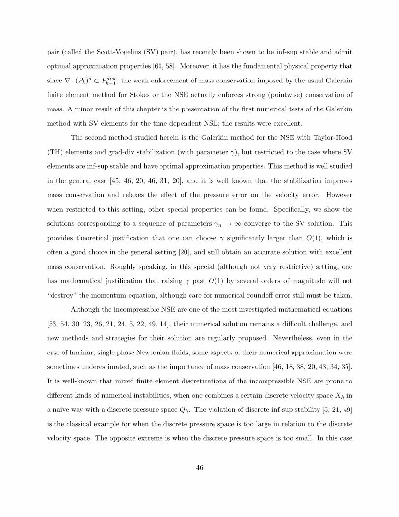
pair (called the Scott-Vogelius (SV) pair), has recently been shown to be inf-sup stable and admit

optimal approximation properties [60, 58]. Moreover, it has the fundamental physical property that

since ∇ · (Pk)d ⊂ P disck−1 , the weak enforcement of mass conservation imposed by the usual Galerkin

finite element method for Stokes or the NSE actually enforces strong (pointwise) conservation of

mass. A minor result of this chapter is the presentation of the first numerical tests of the Galerkin

method with SV elements for the time dependent NSE; the results were excellent.

The second method studied herein is the Galerkin method for the NSE with Taylor-Hood

(TH) elements and grad-div stabilization (with parameter γ), but restricted to the case where SV

elements are inf-sup stable and have optimal approximation properties. This method is well studied

in the general case [45, 46, 20, 46, 31, 20], and it is well known that the stabilization improves

mass conservation and relaxes the effect of the pressure error on the velocity error. However

when restricted to this setting, other special properties can be found. Specifically, we show the

solutions corresponding to a sequence of parameters γn → ∞ converge to the SV solution. This

provides theoretical justification that one can choose γ significantly larger than O(1), which is

often a good choice in the general setting [20], and still obtain an accurate solution with excellent

mass conservation. Roughly speaking, in this special (although not very restrictive) setting, one

has mathematical justification that raising γ past O(1) by several orders of magnitude will not

“destroy” the momentum equation, although care for numerical roundoff error still must be taken.

Although the incompressible NSE are one of the most investigated mathematical equations

[53, 54, 30, 23, 26, 21, 24, 5, 22, 49, 14], their numerical solution remains a difficult challenge, and

new methods and strategies for their solution are regularly proposed. Nevertheless, even in the

case of laminar, single phase Newtonian fluids, some aspects of their numerical approximation were

sometimes underestimated, such as the importance of mass conservation [46, 18, 38, 20, 43, 34, 35].

It is well-known that mixed finite element discretizations of the incompressible NSE are prone to

different kinds of numerical instabilities, when one combines a certain discrete velocity space Xh in

a naive way with a discrete pressure space Qh. The violation of discrete inf-sup stability [5, 21, 49]

is the classical example for when the discrete pressure space is too large in relation to the discrete

velocity space. The opposite extreme is when the discrete pressure space is too small. In this case

46

the approximation does not adequately satisfy the conservation of mass equation, thereby giving

a poor approximation to the physical solution. It is this second problem that is the motivation of

this work.

There are a number of strategies for avoiding poor mass conservation: several element

choices are known provide pointwise mass conservation [60, 58], discontinuous Galerkin methods

admit local mass conservation [48], penalization techniques such as grad-div stabilization discussed

herein reduce global mass conservation error, and a posteriori methods can be used to enforce the

conservation of mass on already computed solutions [41]. For each technique, there are naturally

both good features and drawbacks, and therefore a determination of which method is “best” is

certainly problem dependent.

Still, in most cases, the use of TH elements with grad-div stabilization is one of the easiest

to implement. For many years TH elements have been a popular choice of approximating element

in fluid flow simulations, with most downloadable finite element packages have some TH elements

implemented. Hence getting a TH code and adding grad-div stabilization is typically convenient

and simple. However, until now, it was believed that the improvement in mass conservation using

grad-div stabilization, although sometimes significant over usual TH solutions, was limited to an

O(1) choice of the stabilization parameter. With this limitation, one had to decide whether the

provided mass conservation was good enough, or instead if a different element choice or DG should

be used instead. Hence this work provides a simple solution to correct for poor mass conservation

in existing codes, and therefore may lead to TH elements being a good choice on a much wider set

of problems.

This chapter is arranged as follows. In Section 2, we give notation and preliminaries,

including a brief discussion of the SV element. Section 3 proves that on barycenter refined meshes

and k ≥ d, grad-div stabilized TH solutions of the NSE converge to SV solutions as the grad-div

parameter tends to ∞. Section 4 presents numerical experiments that illustrate the theory.

47

4.2 Preliminaries

We will represent the L2 norm and inner product by ‖·‖ and (·, ·), respectively. All other

norms used will be clearly denoted with subscripts.

Recall the time dependent incompressible NSE on a polygonal (2d), or polyhedral (3d),

domain Ω, and for simplicity with homogeneous Dirichlet boundary conditions:

ut − ν∇u + u · ∇u +∇p = f , in Ω× (0, T ], (4.1)

∇ · u = 0, in Ω× (0, T ], (4.2)

u(x, 0) = u0, in Ω (4.3)

u = 0 on ∂Ω× (0, T ]. (4.4)

Here, u represents velocity, p the (zero-mean) pressure, f an external force, and ν the kinematic

viscosity.

Throughout the report, (Xh, Qh) ⊂ (H10 (Ω), L2

0(Ω)) will denote either the Taylor-Hood or

Scott-Vogelius element pair. Due to the assumptions that the approximating polynomial degree

k ≥ d and the mesh be constructed by a barycenter refinement of a quasi-uniform mesh (details in

the following section), (Xh, Qh) will be inf-sup stable.

The following lemma will be used in the analysis that follows.

Lemma 4.2.1. There exists a constant C∗(Ω), dependent only on the size of Ω, that satisfies

∀u, v, w ∈ H10 (Ω),

|(u · ∇v, w)|+ |((∇ · u)v, w)| ≤ C∗ ‖∇u‖ ‖∇v‖ ‖∇w‖1/2 ‖w‖1/2 (4.5)

|(u · ∇v, w)|+ |((∇ · u)v, w)| ≤ C∗ ‖∇u‖ ‖∇v‖ ‖∇w‖ (4.6)

Proof. The first inequality follows from Holder’s inequality, Ladyzhenskaya inequalities and the

Sobolev imbedding theorem. The second follows directly from the first with the Poincare inequality

in H10 (Ω).

48

4.2.1 Scott-Vogelius and Taylor-Hood elements

The SV element pair is not yet very well known, and so we now give a brief description of

it. In essence, the SV pair is the same as the TH pair except that

(i) k ≥ d, where d is the space dimension,

(ii) the pressure space is discontinuous, and

(iii) the mesh is required to be a barycenter refinement of a regular mesh.

That is, polynomials of degree k and k−1 are used to approximate the velocity and pressure spaces

respectively, with k ≥ d (which is only a restriction in 3d compared to TH), and the mesh Th

that is used must be derived from a regular triangularization (tetrahedralization) of Ω, where each

element is refined by connecting its barycenter to the vertices. An illustration of such a refinement

is given in Figure 4.1. With such a mesh construction and k ≥ d, it was proved by Zhang in [58]

that the SV elements are LBB stable under these restrictions. It is well known that the TH pair is

LBB stable for this case [21].

Figure 4.1: (LEFT) 2d and (RIGHT) 3d macro-element, shown with dashed lines representingbarycenter refinements

We now formally define the element pairs. In space dimension d, for both Taylor-Hood and

Scott-Vogelius elements we define Xh to be the space of continuous element-wise vector functions

of polynomial order k ≥ d on Th

Xh :=

vh ∈ [C(Ω)]d : vh|T ∈ [Pk(T )]d, for all T ∈ Th , vh = 0 on ∂Ω.

49

For Taylor-Hood, we define

QTHh :=

qh ∈ L2(Ω) ∩ C(Ω): qh|T ∈ Pk−1, for all T ∈ Th

,

while the pressure space of the Scott-Vogelius element is only different from Taylor-Hood’s in that

its pressures are discontinuous:

QSVh :=

qh ∈ L2(Ω): qh|T ∈ Pk−1, for all T ∈ Th

.

Note that the dimension of the pressure space for SV elements is significantly larger than that for

TH elements. This creates a greater total number of degrees of freedom needed for linear solves

using SV elements, however it is not immediately clear whether this will lead to a significant increase

in computational time if preconditioners such as Augmented Lagrangian type are used [4]. The

authors plan to consider this questions in future studies.

Although the velocity spaces of the TH and SV elements are the same, the spaces of dis-

cretely divergence free subspaces are different, and will be denoted by

V SVh := vh ∈ Xh : (∇ · vh, qh) = 0 ∀qh ∈ QSVh

V THh := vh ∈ Xh : (∇ · vh, qh) = 0 ∀qh ∈ QTHh .

The SV element is very interesting from the mass conservation point of view since its discrete

velocity space and its discrete pressure space fulfill an important property, namely

∇ ·Xh ⊂ QSVh . (4.7)

Thus, using SV elements, weak mass conservation via

(∇ · uh, qh) = 0 ∀qh ∈ Qh

implies strong (pointwise) mass conservation since we can choose the special test function qh = ∇·uh

50

to get

‖∇ · uh‖2 = 0 .

In general, the same pressure test function cannot be used in the Taylor-Hood case, since ∇ ·Xh 6⊂

QTHh . Hence the Taylor-Hood element only delivers discretely divergence-free approximations uh.

The temporal-spatial discretization we study, for either TH or SV, is the Crank-Nicolson

Galerkin method, given in skew-symmetrized form by:

Find (unh, pnh) ∈ Xh×Qh with Qh ∈ QTH

h , QSVh such that ∀(vh, qh) ∈ Xh×Qh for n = 1, 2, . . . ,M =

T/∆t,

1∆t

(un+1h − unh,v)− (p

n+ 12

h ,∇ · vh) + ν(∇un+ 1

2h ,∇vh) + γ(∇ · un+ 1

2h ,∇ · vh)

+(un+ 1

2h · ∇u

n+ 12

h ,vh) +12

((divun+ 1

2h )u

n+ 12

h ,vh) = (fn+ 12 ,vh) (4.8)

(∇ · un+1h , qh) = 0 . (4.9)

For the discrete initial velocity, u0h we impose zero pointwise divergence for the initial condition for

both SV or TH elements: ∀(vh, qh) ∈ (Xh, QSVh ),

(u0h,vh) + (λh,∇ · vh) + (∇ · u0

h, qh) = (u0,vh) . (4.10)

This condition is necessary for TH elements due to the Crank-Nicolson temporal discretization and

our enforcement of discrete mass conservation (4.9). For the backward Euler method, this would

not be necessary. However, it is easy to implement.

Note that for SV elements, the term arising from skew-symmetrization vanishes, and is not

necessary to use in computations.

51

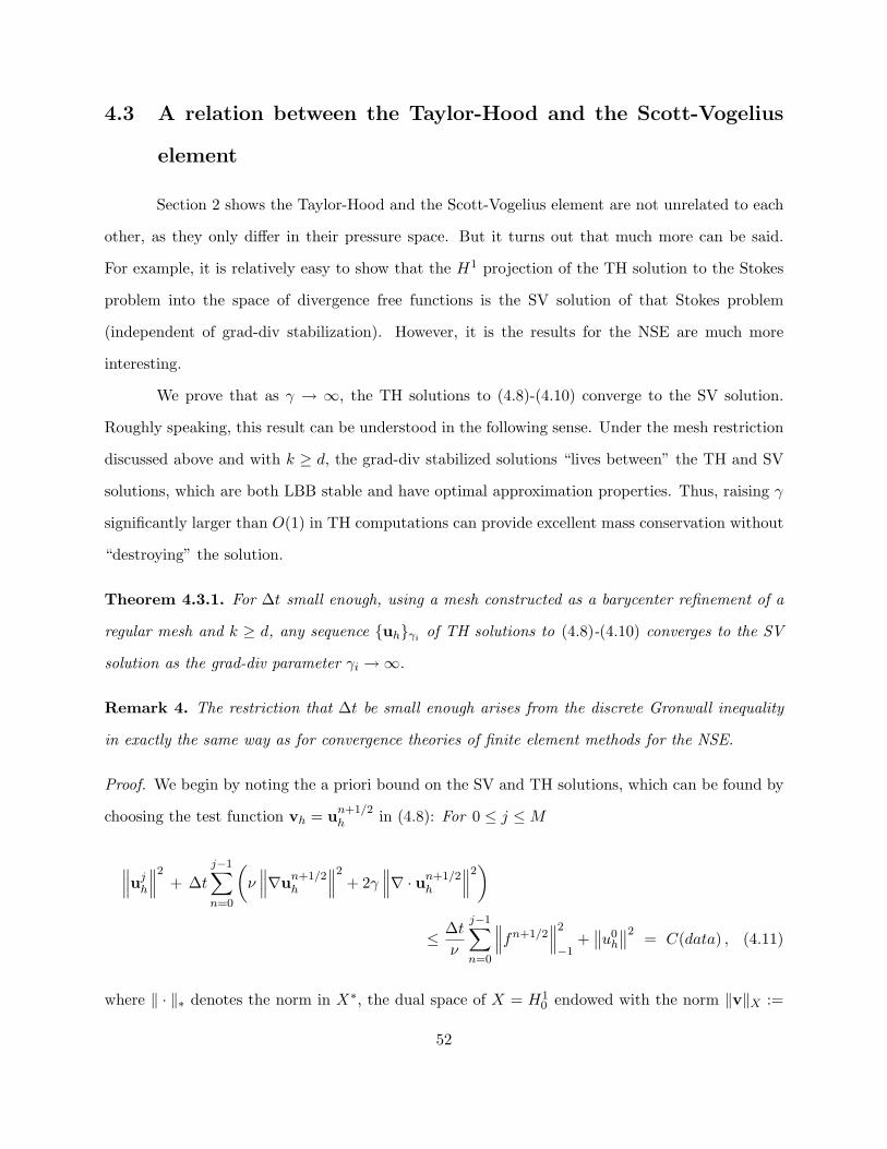
4.3 A relation between the Taylor-Hood and the Scott-Vogelius

element

Section 2 shows the Taylor-Hood and the Scott-Vogelius element are not unrelated to each

other, as they only differ in their pressure space. But it turns out that much more can be said.

For example, it is relatively easy to show that the H1 projection of the TH solution to the Stokes

problem into the space of divergence free functions is the SV solution of that Stokes problem

(independent of grad-div stabilization). However, it is the results for the NSE are much more

interesting.

We prove that as γ → ∞, the TH solutions to (4.8)-(4.10) converge to the SV solution.

Roughly speaking, this result can be understood in the following sense. Under the mesh restriction

discussed above and with k ≥ d, the grad-div stabilized solutions “lives between” the TH and SV

solutions, which are both LBB stable and have optimal approximation properties. Thus, raising γ

significantly larger than O(1) in TH computations can provide excellent mass conservation without

“destroying” the solution.

Theorem 4.3.1. For ∆t small enough, using a mesh constructed as a barycenter refinement of a

regular mesh and k ≥ d, any sequence uhγi of TH solutions to (4.8)-(4.10) converges to the SV

solution as the grad-div parameter γi →∞.

Remark 4. The restriction that ∆t be small enough arises from the discrete Gronwall inequality

in exactly the same way as for convergence theories of finite element methods for the NSE.

Proof. We begin by noting the a priori bound on the SV and TH solutions, which can be found by

choosing the test function vh = un+1/2h in (4.8): For 0 ≤ j ≤M

∥∥∥ujh∥∥∥2+ ∆t

j−1∑n=0

(ν∥∥∥∇un+1/2

h

∥∥∥2+ 2γ

∥∥∥∇ · un+1/2h

∥∥∥2)

≤ ∆tν

j−1∑n=0

∥∥∥fn+1/2∥∥∥2

−1+∥∥u0

h

∥∥2 = C(data) , (4.11)

where ‖ · ‖∗ denotes the norm in X∗, the dual space of X = H10 endowed with the norm ‖v‖X :=

52

‖∇v‖. (For the SV solution∥∥∥∇ · un+1/2

h

∥∥∥2= 0.) This bound is sufficient to show, using the

Leray-Schauder fixed point theorem, that solutions to (4.8)-(4.10) exist for either element pair [30].

Since the timestep and mesh are fixed, uniqueness follows from the boundedness of solutions shown

above.

In addition, by assumption of the existence of the SV solution (which is independent of γ)

and LBB stability we have the SV pressure is bounded independent of γ. In particular we have

that for 2 ≤ j ≤M

∆tj−1∑n=0

∥∥∥pn+1/2SV

∥∥∥2≤ C(data) . (4.12)

Note that from (4.11) it follows that as γ →∞, ∇ · un+1/2h → 0 for n = 0, . . .M − 1. Also,

as ∇ ·u0h = 0, then ∇ ·un+1

h → 0 for n = 0, . . .M − 1. In addition, as∥∥∥ujh∥∥∥2

is uniformly bounded,

then the terms∥∥∥∇ujh

∥∥∥2and

∥∥∥∇ · ujh∥∥∥2are also uniformly bounded. In these later cases the bound

will depend upon the mesh parameter h. However, as we are discussing convergence on a fixed

mesh, this dependence is not important.

Let e := uSV − uTH ∈ V THh , where (uSV , pSV ) and (uTH , pTH) denote the SV and TH

solutions respectively. (For convenience, in this proof we suppress the dependence on h.)

For v ∈ V THh , we have that (p

n+ 12

TH ,∇ · v) = 0 and thus that

1∆t

(en+1 − en,v)− (pn+ 1

2SV ,∇ · v) + ν(∇en+ 1

2 ,∇v) + γ(∇ · en+ 12 ,∇ · v)

+(un+ 1

2SV · ∇u

n+ 12

SV ,v)− (un+ 1

2TH · ∇u

n+ 12

TH ,v) +12

((divun+ 1

2SV )u

n+ 12

SV ,v)

−12

((divun+ 1

2TH )u

n+ 12

TH ,v) = 0 , (4.13)

which can be written as

1∆t

(en+1 − en,v) + ν(∇en+ 12 ,∇v) + γ(∇ · en+ 1

2 ,∇ · v)

= −(en+1/2 · ∇un+ 1

2SV ,v) − (u

n+ 12

TH · ∇en+1/2,v)− 12

((diven+1/2)un+ 1

2SV ,v)

−12

((divun+ 1

2TH )en+1/2,v) + (p

n+ 12

SV ,∇ · v) . (4.14)

53

With v = en+ 12 , the identity

(un+ 1

2TH · ∇en+1/2, en+ 1

2 ) +12

((divun+ 1

2TH )en+1/2, en+ 1

2 ) = 0 ,

and using Lemma 4.2.1, equation (4.14) becomes

12∆t

(∥∥en+1

∥∥2 − ‖en‖2) + ν∥∥∥∇en+1/2

∥∥∥2+ γ

∥∥∥∇ · en+1/2∥∥∥2

= −12

((diven+ 12 )u

n+ 12

SV , en+1/2)− (en+ 12 · ∇u

n+ 12

SV , en+1/2) + (pn+ 1

2SV ,∇ · en+1/2)

≤ C∥∥∥∇en+1/2

∥∥∥2 ∥∥∥∇un+1/2SV

∥∥∥+∥∥∥∥pn+ 1

2SV

∥∥∥∥∥∥∥∇ · en+1/2∥∥∥ . (4.15)

Since the mesh is fixed, uniform boundedness, finite dimensionality of un+ 1

2SV , and Young’s inequality

imply

12∆t

(∥∥en+1

∥∥2 − ‖en‖2) + ν∥∥∥∇en+1/2

∥∥∥2+ γ

∥∥∥∇ · en+1/2∥∥∥2

≤ C∥∥∥en+1/2

∥∥∥2+γ

2

∥∥∥∇ · en+1/2∥∥∥2

+1

2γ

∥∥∥pn+1/2SV

∥∥∥2. (4.16)

With∥∥e0∥∥ = 0, subtracting γ

2

∥∥∇ · en+1/2∥∥2

from both sides of (4.16), then summing from n = 0

to j − 1, 2 ≤ j ≤M , we have

∥∥ej∥∥2 + ∆tj−1∑n=0

(2ν∥∥∥∇en+1/2

∥∥∥2+ γ

∥∥∥∇ · en+1/2∥∥∥2)

≤ C∆tj∑

n=0

‖en‖2 +∆tγ

j−1∑n=0

∥∥∥pn+1/2SV

∥∥∥2. (4.17)

The discrete Gronwall inequality [25] then implies that (for ∆t sufficiently small)

∥∥ej∥∥2 + ∆tj−1∑n=0

(2ν∥∥∥∇en+1/2

∥∥∥2+ γ

∥∥∥∇ · en+1/2∥∥∥2)≤ C

∆tγ

j−1∑n=0

∥∥∥pn+1/2SV

∥∥∥2

≤ C1γ.

Hence, as γ →∞,∥∥ej∥∥→ 0, j = 1, 2, . . . ,M , i.e. uTH → uSV .

54

4.3.1 A connection for the steady NSE problem

An analogous result as proved above holds for the steady NSE. Consider the usual skew

symmetrized finite element scheme for the NSE [30]: Find (uh, ph) ∈ (Xh, Qh) satisfying ∀(vh, qh) ∈

(Xh, Qh)

ν(∇uh,∇vh)− (ph,∇ · vh) + γ(∇ · uh,∇ · vh) + (uh · ∇uh,vh)

+12

((divuh)uh,vh) = (f ,vh), (4.18)

(∇ · uh, qh) = 0, (4.19)

where Qh is either QSVh or QTHh . Note if Qh = QSVh , then trivially 12((divuh)uh,vh) = γ(∇·uh,∇·

vh) = 0. It is not hard to show that solutions to (4.18) exist with the Leray-Schauder fixed point

theorem, and under the small data condition C∗ν−2 ‖f‖−1 < 1 (where C∗ = C∗(Ω) is from Lemma

4.2.1), solutions are also unique [30].

Theorem 4.3.2. Suppose the data in the problem (4.18)-(4.19) satifies α := C∗ν−2 ‖f‖−1 < 1.

Then for any sequence of grad-div stabilization parameters γi →∞, the corresponding TH solutions

converge to the SV solution.

Proof. Proceeding in an analogous manner as in the proof of Theorem 4.3.1, note that by choosing

vh = uh

ν ‖∇uh‖2 + 2γ ‖∇ · uh‖2 ≤ ν−1 ‖f‖2−1 = C(data). (4.20)

From (4.20) we have uniform boundedness of uh (with respect to γ) by the Poincare-Friedrichs

inequality, and thus uniform boundedness of eh.

Following similar to the time dependent case, we have that eh satisfies

ν ‖∇e‖2 + γ ‖∇ · e‖2 ≤ C∗ ‖∇uSV ‖ ‖∇e‖2 +γ

2‖∇ · e‖2 +

12γ‖pSV ‖2

≤ C∗ν−1 ‖f‖−1 ‖∇e‖2 +γ

2‖∇ · e‖2 +

12γ‖pSV ‖2 , (4.21)

55

and thus

(ν − C∗ν−1 ‖f‖−1) ‖∇e‖2 +γ

2‖∇ · e‖2 ≤ 1

2γ‖pSV ‖2 . (4.22)

Using the small data condition, this reduces to

‖∇e‖2 ≤ C

γ‖pSV ‖2 , (4.23)

which implies e→ 0 as γ →∞.

4.4 2D Numerical Experiments

In this section we investigate the convergence theory of the previous section and the theory

that NSE approximations using TH elements with large grad-div stabilization parameters will

provide both good mass conservation and accurate solutions (when the SV solution is accurate), if

k ≥ d and with the mesh restriction discussed in Section 2. Indeed we find this is the case.

4.4.1 Numerical Experiment 1: 2d channel flow around a cylinder on a barycen-

ter refined mesh

The benchmark problem of 2D channel flow around a cylinder has been studied in numerous

works, e.g. [50, 27, 29, 31], and is well documented in [50]. The domain is the rectangle [0, 2.2] ×

[0, 0.41] representing the channel with flow in the positive x direction, with a circle radius 0.05

centered at (0.2, 0.2) representing the cylinder. No slip boundary conditions are prescribed on the

top and bottom of the channel as well as on the cylinder, and the time dependent inflow and outflow

velocity profiles are given by

u(0, y, t) = u(2.2, y, t) =[

60.412

sin(πt/8)y(0.41− y) , 0]T, 0 ≤ y ≤ 0.41.

The forcing function is set to zero, f = 0, and the viscosity at ν = 0.001, providing a time dependent

Reynolds number, 0 ≤ Re(t) ≤ 100. The initial condition is u = 0, and we compute to end-time

56

T = 8 with time-step ∆t = 0.01.

An accurate approximation of this flow’s velocity field will show a vortex street forming

behind the cylinder by t = 4, and a fully formed vortex street by t = 7. However, there is more

than one way to measure accuracy. That is, even if the vortex street forms and the velocity vector

field “appears” correct, if the velocity field does not conserve mass, then for many applications the

solution may be unacceptable.

Solutions are computed for (P2, Pdisc1 ) SV elements and for (P2, P1) TH elements with

γ = 0, 1, 100, 10, 000, all on the same barycenter refined mesh. This provides 6,578 velocity

degrees of freedom and 4,797 pressure degrees of freedom for the SV pressure, and 845 pressure

degrees of freedom for the TH simulation. Results of these simulations are shown in Table 4.1, and

Figures 4.2 and 4.3.

γ∥∥∇uγTH(t = 7)−∇uSV (t = 7)

∥∥0 5.70861 0.7616

100 7.9856e-310,000 8.5311e-5

Table 4.1: The table above shows convergence of the grad-div stabilized TH approximations to theSV approximation for numerical experiment 1.

Table 4.1 shows convergence of the TH approximations to the SV approximation as γ →∞.

This agrees with the theory of Section 3. Figure 4.2 shows the plots of the velocity field, speed

contours and pressure contours for SV and TH approximations with γ = 0, 1, 100, 10, 000. The

convergence as γ gets large of the TH approximations to the SV approximation is clear. We note

the dramatic improvement for the TH approximation from changing γ = 0 to γ = 1, continuing

to raise γ increases the accuracy further, until by γ = 10, 000 when a very good approximation is

found.

The benefit to mass conservation of increasing γ is shown in figure 4.3. Here we see with

γ = 10, 000, excellent mass conservation is achieved. Also we note that for the unstabilized TH

approximation, ‖∇ · unh‖ = O(1).

57

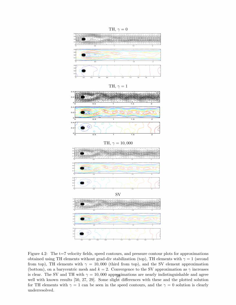
TH, γ = 0

0 0.5 1 1.5 20

0.1

0.2

0.3

0.4

0 0.5 1 1.5 20

0.1

0.2

0.3

0.4

0 0.2 0.4 0.6 0.8 1 1.2 1.4 1.6 1.8 20

0.1

0.2

0.3

0.4

TH, γ = 1

0 0.5 1 1.5 20

0.2

0.4

0 0.5 1 1.5 20

0.2

0.4

0 0.5 1 1.5 20

0.2

0.4

TH, γ = 10, 000

0 0.5 1 1.5 20

0.1

0.2

0.3

0.4

0 0.5 1 1.5 20

0.1

0.2

0.3

0.4

0 0.5 1 1.5 20

0.1

0.2

0.3

0.4

SV

0 0.5 1 1.5 20

0.1

0.2

0.3

0.4

0 0.5 1 1.5 20

0.1

0.2

0.3

0.4

0.2 0.4 0.6 0.8 1 1.2 1.4 1.6 1.8 2

0.1

0.2

0.3

0.4

Figure 4.2: The t=7 velocity fields, speed contours, and pressure contour plots for approximationsobtained using TH elements without grad-div stabilization (top), TH elements with γ = 1 (secondfrom top), TH elements with γ = 10, 000 (third from top), and the SV element approximation(bottom), on a barycentric mesh and k = 2. Convergence to the SV approximation as γ increasesis clear. The SV and TH with γ = 10, 000 approximations are nearly indistinguishable and agreewell with known results [50, 27, 29]. Some slight differences with these and the plotted solutionfor TH elements with γ = 1 can be seen in the speed contours, and the γ = 0 solution is clearlyunderresolved.

58

0 1 2 3 4 5 6 7 810 20

10 15

10 10

10 5

100

105

t

||

u hn ||

L2 norm of divergence of computed velocities against time

Taylor Hood, =0Taylor Hood, =1Taylor Hood, =100Taylor Hood, =10,000Scott Vogelius

Figure 4.3: Shown above are the plots of ‖∇ · unh‖ vs. time for the SV and TH approximations fornumerical experiment 1, with varying γ.

4.4.2 Numerical Experiment 2: The 3d driven cavity

In 3d, SV elements require k ≥ 3. Here we compare the (P3, Pdisc2 ) SV approximation with

that obtained using by grad-div stabilized (P3, P2) TH elements.

We consider the benchmark problem of the 3D lid-driven cavity. This problem has been

well-studied, [57, 44], and the description is as follows. The domain Ω is the (−1, 1)3 cube, for

boundary conditions the top of the box (lid) is prescribed the velocity u = [1, 0, 0]T with the

velocity on the the sides and bottom set to zero (u = 0), and the viscosity ν = 1/50, giving the

Reynolds’ number Re = 2 · 1 · 50 = 100. We compute with a barycenter refinement of a uniform

tetrahedral mesh (as discussed in Section 2), consisting of 51,119 total dof for the TH elements

(46,038 velocity and 5,081 pressure) and 76,038 total dof for SV elements (46,038 velocity and

30,000 pressure). The problem is solved directly for the steady state approximation with a Newton

iteration, using as the initial guess u(x) = 0, x ∈ Ω. Five iterations were required to converge to a

tolerance of 10−10 for each of the tests. We compare the SV approximation and TH approximations

with stabilization parameters γ = 0, 1, 100, 10, 000. Plots of the approximations are presented in

59

x

y

x

z

y

z

x

z

0 0.5 1 1.5 2x 10 14

y

z

1.5 1 0.5 0 0.5 1x 10 14

y

x

5 0 5x 10 15

Midplane velocity fields and divergence contours for Scott Vogelius elt solution

Figure 4.4: We see the expected velocity profiles for the lid-driven cavity problem with div uh closeto machine epsilon.

Figures 4.4-4.8.

Comparing the plots of the midplane velocity fields (Figures 4.4-4.8) with the documented

solution [57, 44], the approximations “appear” correct. As noted in the the 2d experiments, the

TH approximations with smaller γ exhibit poor mass conservation. In Figure 4.4, as expected, we

see pointwise mass conservation for the SV element solution. In Figure 4.5 (γ = 0), we observe

only O(10−1) mass conservation. Figure 4.6 shows that γ = 1 improves the mass conservation

to O(10−2), and more grad-div stabilization (i.e. larger γ) further improves mass conservation as

shown in Figures 4.7 and 4.8.

The convergence of the TH velocity approximations to the SV velocity approximation can

be seen in Table 4.2, giving verification to the theory of Section 3.

60

x

y

x

z

y

z

x

z

1 0.5 0

y

z

0.2 0 0.2

x

y

0.06 0

Midplane velocity fields and divergence contours for Taylor Hood elt solution

Figure 4.5: For TH with γ = 0, we see the expected velocity profiles for the lid-driven cavityproblem, with non-negligible error for div uh.

γ∥∥∇uγTH −∇uSV

∥∥0 1.06531 0.2093

100 0.002910,000 2.951e-5

Table 4.2: Convergence of the grad-div stabilized TH approximations toward the SV approximationas γ →∞ for the Re = 100 3d driven cavity problem.

4.5 Conclusions and Future Directions

By proving (and then exploiting) a connection between Scott-Vogelius and grad-div stabi-

lized Taylor Hood approximations of the NSE, we have shown that under a mild mesh restriction

and by choosing the approximating polynomial degree k ≥ d, grad-div stabilization can have a

much greater positive effect on Taylor-Hood approximations than previously believed. In this situ-

61

1 0.5 0 0.5 11

0.8

0.6

0.4

0.2

0

0.2

0.4

0.6

0.8

1

x

y

1 0.5 0 0.5 11

0.8

0.6

0.4

0.2

0

0.2

0.4

0.6

0.8

1

x

z

1 0.5 0 0.5 11

0.8

0.6

0.4

0.2

0

0.2

0.4

0.6

0.8

1

y

z

x

y

8 6 4 2 0 2 4x 10 3

x

z

0.05 0 0.05 0.1

y

z

0.01 0 0.01

Midplane Velocity Fields and Divergence Contours for TH =1

Figure 4.6: For TH with γ = 1, we see the expected velocity profiles for the lid-driven cavityproblem with non-negligible error for div uh.

ation, we are able to raise the stabilization parameter larger than O(1), thus achieving much better

mass conservation.

We have also shown that Scott-Vogelius elements can be an excellent choice for approxi-

mating solutions to the NSE. To our knowledge, these are the first tests of this element pair on the

time dependent Navier-Stokes equation.

Due to the similarity of Taylor-Hood elements and Scott-Vogelius elements, many existing

codes using Taylor-Hood elements can be easily converted to use Scott-Vogelius elements (provided

the mesh is as specified above). Hence we believe this element may be of great interest to engineers

and fluid dynamicists interested in better mass conservation with reasonable development cost.

62

x

y

x

z

Midplane Velocity Fields and Divergence Contours for TH =100

y

z

x

y

5 0 5x 10 5

x

z

5 0 5 10x 10 4

y

z

1 0 1x 10 4

Figure 4.7: For TH with γ = 100, we see the expected velocity profiles for the lid-driven cavityproblem with improved error for div uh.

63

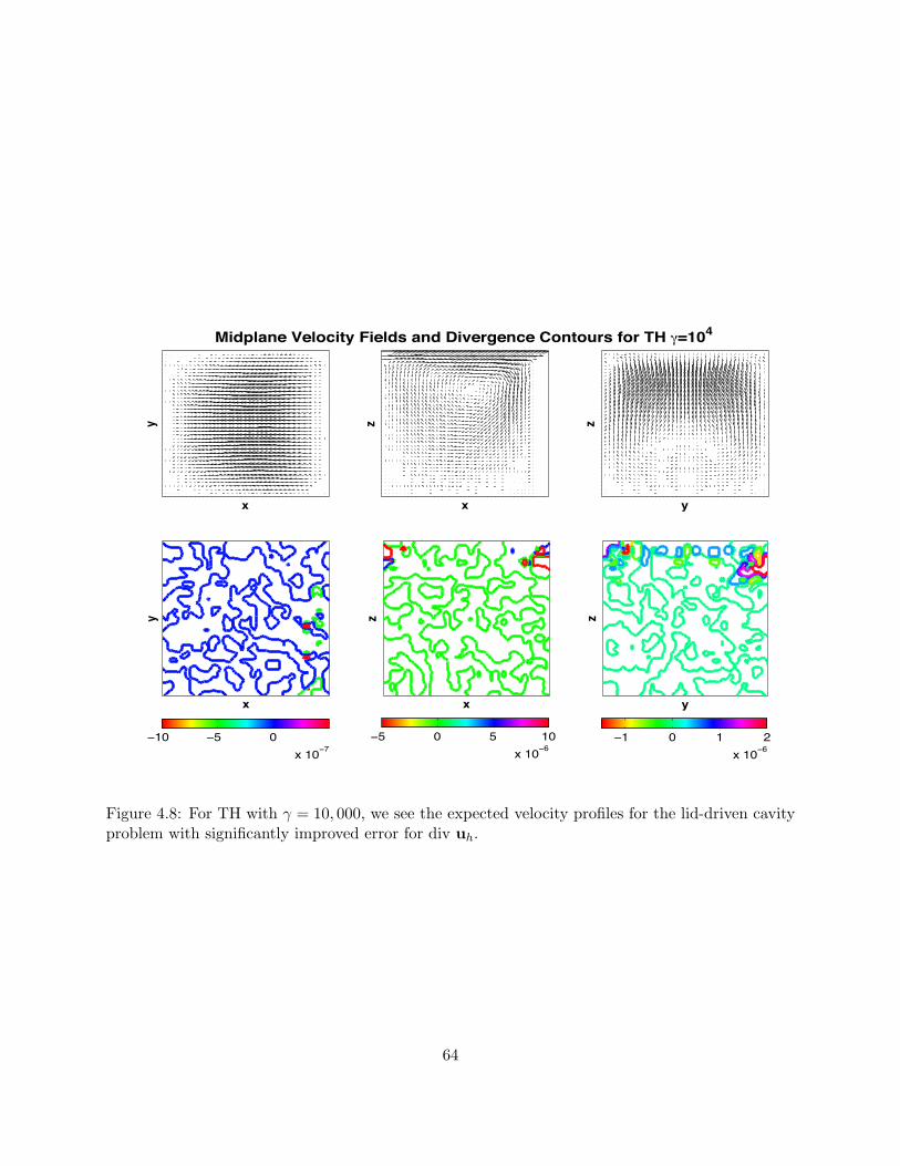
x

y

x

z

Midplane Velocity Fields and Divergence Contours for TH =104

y

z

x

y

10 5 0x 10 7

x

z

5 0 5 10x 10 6

y

z

1 0 1 2x 10 6

Figure 4.8: For TH with γ = 10, 000, we see the expected velocity profiles for the lid-driven cavityproblem with significantly improved error for div uh.

64

Chapter 5

An enhanced physics numerical

scheme for MHD

5.1 Introduction

The study of magnetohydrodynamics (MHD) pertains to the interaction of fluid flow and

magnetic fields. In order for the interaction of the fluid and magnetic field to be substantial, the

fluids in question must be conductors and non-magnetic, which leads to the fields of study being salt

water, liquid metals, plasmas and strong electrolytes. MHD is perhaps best known for its association

with colossal failures in power generation, however in the last 30 years, it has been found to be

pertinent to the flow of liquid sodium coolants in fast-breeder reactors, and the confinement of hot

plasma thru magnetic forces during controlled thermonuclear fusion. Furthermore, magnetic fields

are often used to heat, pump, stir and levitate liquid metals in the metallurgical industries [11].

The MHD conservation equations are given in magnetic field form by

ut +∇ · (uuT )−Re−1∆u+S

2∇(B ·B)− S∇ ·BBT +∇p = f, (5.1)

∇ · u = 0, (5.2)

Bt +Re−1m ∇× (∇×B) +∇× (B × u) = ∇× g, (5.3)

∇ ·B = 0, (5.4)

65

where u is velocity, p is pressure, f is body forces such as gravity, ∇× g is a force on the magnetic

field B, Re is the Reynolds number, Rem is the magnetic Reynolds number, and S is the coupling

number.

It is often the case that a careful treatment (or sometimes a clever trick) in the design

of a numerical scheme to simulate physical phenomena can provide more physically relevant and

accurate solutions. In particular, most schemes for fluid flow conserve energy, but there is often

a second fundamental integral variant that is ignored. However, when this second quantity is

accounted for in the design of the numerical scheme, the resulting scheme admits solutions with

greater physical accuracy. The improved physical accuracy may not be evident over small time

intervals but will ultimately manifest itself as time progresses. For example, Arakawas scheme

for the 2D Navier-Stokes equations(NSE) that conserves energy and enstrophy[1], Arakawa and

Lambs scheme for the shallow water equations that conserves enstrophy and potential enstrophy

[2] and those of Navon [41, 42], J.G. Liu and W. Wangs schemes for 3D axi-symmetric NSE flow

that conserves energy and helicity [36] and 3D axi-symmetric MHD flow that conserves energy and

cross-helicity, and most recently a scheme for full 3D NSE that conserves energy and helicity [47],

all exhibit better long time behavior than comparable schemes that conserve only energy.

This paper presents a study of a new Crank-Nicholson Galerkin finite element method

(FEM) for incompressible MHD in general domains. It is the first to accurately treat both energy

and cross-helicity, in the sense of global conservation, on general domains; as mentioned above,

a scheme for axi-symmetric MHD flow was created in [36]. Moreover, with a carefully derived

formulation and choice of finite elements, the scheme is also able to enforce pointwise mass conser-

vation and pointwise enforcement of the magnetic field’s incompressibility. Therefore, the proposed

discrete scheme has the potential for excellent physical accuracy of its discrete solutions and there-

fore for long-time accuracy. We formally prove the conservation properties as well as stability and

convergence for the scheme. Linearized extensions of the proposed scheme, which still preserve the

same quantities, are also discussed.

This report is arranged as follows. Section 2 presents notation and preliminaries, section 3

derives the numerical scheme and proves conservation properties for it. Section 4 presents stability

66

and convergence analysis for the scheme, and section 5 discusses extensions of the scheme to a

linearized form that still admits the conservation properties.

5.2 Notation and Preliminaries

We consider a polygonal or polyhedral domain Ω, with homogeneous Dirichlet boundary

conditions for both velocity and the magnetic field. Extension to periodic boundaries is trivial,

but requires the domain be a box, and extension to most other boundary conditions is done in the

usual way.

We will denote the L2(Ω) norma and inner product by ‖·‖ and (·, ·), respectively.

We will utilize the Poincare-Freidrich’s inequality through our analysis: For φ ∈ H10 (Ω),

‖φ‖ ≤ C(Ω) ‖∇φ‖ .

The continuous function spaces natural for this problem are

X = H10 (Ω) = v ∈ H1(Ω) : v = 0 on ∂Ω

Q = L20(Ω) = q ∈ L2(Ω) :

∫Ωq = 0

The following lemma for bounding the trilinear forms will be used heavily in our analysis.

Lemma 5.2.1. For u, v, w ∈ X, there exists C = C(Ω) such that

(u · ∇v, w) ≤ C ‖∇u‖ ‖∇v‖ ‖v‖1/2 ‖∇v‖1/2 (5.5)

(u · ∇v, w) ≤ C ‖∇u‖ ‖∇v‖ ‖∇v‖ (5.6)

Proof. These estimates follow from Holder’s inequality, the Sobolev imbedding theorem and Poincare-

Freidrich’s inequality.

The finite element spaces used throughout will be the Scott-Vogelius pair, (Xh, Qh) =

(Pk, P disck−1 ), where it is required that k ≥ dim and the mesh be constructed as a barycenter re-

67

finement of a regular mesh. Under these conditions, it is known that this element pair is LBB

stable [58]. This pair will be used to approximate the velocity-vorticity pair, and the magnetic

field - lagrange multiplier pair. A fundamentally important property of this pair is that the usual

Galerkin weak enforcement of incompressibility of an element vh ∈ Xh via

(∇ · vh, qh) = 0∀qh ∈ Qh,

implicitly enforces incompressibility pointwise since qh can be chosen to be ∇ · vh, which provides

‖∇ · vh‖2 = 0 =⇒ ∇ · vh = 0

This is important in our proposed numerical scheme for three reasons. First, mass conservation can

be enforced pointwise via the usual weak enforcement of incompressibility of velocity. Second, the

incompressibility of the magnetic field can be enforced pointwise in the same manner; the magnetic

field equation is derived from by taking the curl of the electric field, and since div of curl is zero,

enforcing this incompressibility is of fundamental importance. Third, in all of our trilinear terms,

skew-symmetry need not be enforced. This will lead to a cheaper assembly of linear systems.

Define the space of discretely divergence free function as

Vh := vh ∈ Xh : (∇ · vh, qh) = 0 ∀qh ∈ Qh.

Note that functions in Vh, when using the Scott-Vogelius pair, are pointwise divergence free.

68

5.3 Derivation of energy and cross-helicity conserving scheme

We begin with the formulation (5.1)-(5.4), expand the curl operator in the (5.3) equation

and use that ∇ · u = ∇ ·B = 0 to get

ut + u · ∇u−Re−1∆u+S

2∇(B ·B)− SB · ∇B +∇p = f (5.7)

∇ · u = 0 (5.8)

Bt +Re−1m ∇× (∇×B) + u · ∇B −B · ∇u = ∇× g (5.9)

∇ ·B = 0 (5.10)

So that (5.10) can be explicitly enforced, the addition of a Lagrange multiplier to (5.9) is done by

adding the (zero) term ∇(∇·B), then substituting λ = ∇·B to get the new set of equations which

has four unknowns and 4 equations,

ut + u · ∇u−Re−1∆u+S

2∇(B ·B)− SB · ∇B +∇p = f (5.11)

∇ · u = 0 (5.12)

Bt +Re−1m ∇× (∇×B) + u · ∇B −B · ∇u+∇λ = ∇× g (5.13)

∇ ·B = 0 (5.14)

From here, we incorporate the homogeneous Dirichlet boundary condition into the function spaces,

and discretize with the Galerkin finite element method and a four-leg Crank-Nicolson temporal

discretization. We denote un+ 1

2h := 1

2(unh + un+1h ), and require the initial u0

h and B0h be in Vh.

Then ∀(vh, χh, qh, rh) ∈ (Xh, Xh, Qh, Qh) find (un+1h , Bn+1

h , pn+ 1

2h , λ

n+ 12

h ) ∈ (Xh, Xh, Qh, Qh) for

69

n = 0, 1, 2, ...,M = T∆t

1∆t

(un+1h − unh, vh) + (u

n+ 12

h · ∇un+ 12

h , vh) +Re−1(∇× un+ 12

h ,∇× vh)

+s

2(B

n+ 12

h ·Bn+ 12

h ,∇ · vh)− s(Bn+ 12

h · ∇Bn+ 12

h , vh)− (pn+ 1

2h ,∇ · vh) = (f(tn+ 1

2 ), vh) (5.15)

(∇ · un+1h , qh) = 0 (5.16)

1∆t

(Bn+1h −Bn

h , χh) +Re−1m (∇×Bn+ 1

2h ,∇× χh)− (B

n+ 12

h · ∇un+ 12

h , χh)

+(un+ 1

2h · ∇Bn+ 1

2h , χh) + (λ

n+ 12

h ,∇ · χh) = (∇× g(tn+ 12 ), χh) (5.17)

(∇ ·Bn+1h , rh) = 0 (5.18)

Lemma 5.3.1. Solutions to the scheme (5.15)-(5.18) admit the following conservation laws:

• Mass conservation

∇ · unh = 0 (pointwise) (5.19)

• Incompressibility of the magnetic field

∇ ·Bnh = 0 (pointwise) (5.20)

• Global energy conservation

(∥∥∥∥12uMh

∥∥∥∥2

+s

2

∥∥BMh

∥∥2

)+ ∆t

M−1∑n=0

(Re−1

∥∥∥∥∇× un+ 12

h

∥∥∥∥2

+ sRe−1m

∥∥∥∥∇×Bn+ 12

h

∥∥∥∥2)

=(

12

∥∥u0h

∥∥2 +s

2

∥∥B0h

∥∥2)

+ ∆tM−1∑n=0

((f(tn+ 1

2 ), un+ 1

2h ) + s(∇× g(tn+ 1

2 ), Bn+ 1

2h )

)(5.21)

• Global cross-helicity conservation

(uMh , BMh ) + ∆t

M−1∑n=0

((Re−1 +Re−1

m )(∇× un+ 12

h ,∇×Bn+ 12

h ))

= (u0h, B

0h) + ∆t

M−1∑n=0

((∇× g(tn+ 1

2 ), un+ 1

2h ) + (f(tn+ 1

2 ), Bn+ 1

2h )

)(5.22)

70

Hence for f = g = 0 and Re = Rem = ∞, we have exact conservation of both energy and

cross-helicity.

Proof. First, we note that for Scott-Vogelius elements, we can choose qh = ∇ · un+1h and rh =

∇ ·Bn+1h . Hence we have that ∇ ·un+1

h = ∇ ·Bn+1h = 0, and thus that ∇ ·un+1/2

h = ∇ ·Bn+1/2h = 0.

This proves the first two conservation laws, and moreover these results will be used in the proofs

of the other laws.

To prove energy conservation choose vh = un+ 1

2h and χh = B

n+ 12

h which vanishes the second,

fourth, and sixth terms in (5.15) and the fourth and fifth terms in (5.17), leaving

12∆t

(∥∥un+1h

∥∥2 − ‖unh‖2)

+Re−1

∥∥∥∥∇× un+ 12

h

∥∥∥∥2

− s(Bn+ 12

h · ∇Bn+ 12

h , un+ 1

2h )

= (f(tn+ 12 ), u

n+ 12

h ), (5.23)

12∆t

(∥∥Bn+1h

∥∥2 − ‖Bnh‖

2)

+Re−1m

∥∥∥∥∇×Bn+ 12

h

∥∥∥∥2

− (Bn+ 1

2h · ∇un+ 1

2h , B

n+ 12

h )

= (∇× g(tn+ 12 ), B

n+ 12

h ). (5.24)

Multiplying (5.24) by s, rewriting the nonlinear term in (5.23) as −s(Bn+ 12

h · ∇Bn+ 12

h , un+ 1

2h ) =

s(Bn+ 1

2h · ∇un+ 1

2h , B

n+ 12

h ), and adding (5.23) and (5.24) gives

12∆t

(∥∥un+1

h

∥∥2 − ‖unh‖) +s

2∆t(∥∥Bn+1

h

∥∥2 − ‖Bnh‖

2) +Re−1

∥∥∥∥∇× un+ 12

h

∥∥∥∥2

+sRe−1m

∥∥∥∥∇×Bn+ 12

h

∥∥∥∥2

= (f(tn+ 12 ), u

n+ 12

h ) + s(∇× g(tn+ 12 ), B

n+ 12

h ). (5.25)

Multipling by ∆t and summing over timesteps finishes the proof of (5.21).

To prove cross helicity is conserved we choose vh = Bn+ 1

2h in (5.15) and χh = u

n+ 12

h in (5.17).

This vanishes the fourth, fifth and sixth terms in (5.17) and the third and fifth terms in (5.15),

leaving

71

1∆t

(un+1h − unh, B

n+ 12

h ) + (un+ 1

2h · ∇un+ 1

2h , B

n+ 12

h ) +Re−1(∇× un+ 12

h ,∇×Bn+ 12

h )

= (f(tn+ 12 ), B

n+ 12

h ), (5.26)

1∆t

(Bn+1h −Bn

h , un+ 1

2h ) +Re−1

m (∇×Bn+ 12

h ,∇× un+ 12

h ) + (un+ 1

2h · ∇Bn+ 1

2h , u

n+ 12

h )

= (∇× g(tn+ 12 ), u

n+ 12

h ). (5.27)

Adding (5.26) and (5.27) and noting that:

• (un+ 1

2h · ∇un+ 1

2h , B

n+ 12

h ) = −(un+ 1

2h · ∇Bn+ 1

2h , u

n+ 12

h ) (5.28)

• 1∆t

(un+1h − unh, B

n+ 12

h ) +1

∆t(Bn+1

h −Bnh , u

n+ 12

h ) (5.29)

=1

2∆t((un+1h , Bn+1

h )− (unh, Bnh ))

+1

2∆t((un+1h , Bn

h )− (unh, Bn+1h )

)(5.30)

+1

2∆t((Bn+1

h , un+1h )− (Bn

h , unh))− 1

2∆t((Bn+1

h , unh)− (Bnh , u

n+1h )

), (5.31)

gives

1∆t((un+1h , Bn+1

h )− (unh, Bnh ))

+ (Re−1 +Re−1m )(∇× un+ 1

2h ,∇×Bn+ 1

2h )

= (∇× g(tn+ 12 ), u

n+ 12

h ) + (f(tn+ 12 ), B

n+ 12

h ) (5.32)

Multiplying by ∆t and summing over timesteps finishes the proof of (5.22).

5.4 Numerical analysis of the scheme

We prove that the scheme is both unconditionally stable and optimally convergent in this

section.

Lemma 5.4.1. Solutions to the scheme (5.15)-(5.18) are stable provided f ∈ L2(0, T ;H−1(Ω)) and

72

g ∈ L2(0, T ;L2(Ω)), and satisfy

(∥∥uMh ∥∥2+ s

∥∥BMh

∥∥2)

+ ∆tM−1∑n=0

(Re−1

∥∥∥∥∇× un+ 12

h

∥∥∥∥2

+ sRe−1m

∥∥∥∥∇×Bn+ 12

h

∥∥∥∥2)

≤(∥∥u0

h

∥∥2 + s∥∥B0

h

∥∥2)

+ ∆tM−1∑n=0

(Re∥∥∥f(tn+ 1

2 )∥∥∥2

−1+ sRem

∥∥∥g(tn+ 12 )∥∥∥2)

= C(data). (5.33)

Proof. We begin this proof with the energy conservation equality (5.21),

(∥∥∥∥12uMh

∥∥∥∥2

+s

2

∥∥BMh

∥∥2

)+ ∆t

M−1∑n=0

(Re−1

∥∥∥∥∇× un+ 12

h

∥∥∥∥2

+ sRe−1m

∥∥∥∥∇×Bn+ 12

h

∥∥∥∥2)

=(

12

∥∥u0h

∥∥2 +s

2

∥∥B0h

∥∥2)

+ ∆tM−1∑n=0

((f(tn+ 1

2 ), un+ 1

2h ) + s(∇× g(tn+ 1

2 ), Bn+ 1

2h )

)(5.34)

The forcing term can be majorized with Cauchy-Schwarz and Young’s inequalities to get

(f(tn+ 12 ), u

n+ 12

h ) ≤ Re

2

∥∥∥f(tn+ 12 )∥∥∥2

−1+Re−1

2

∥∥∥∇un+1/2h

∥∥∥2, (5.35)

and similarly for the magnetic forcing term,

s(∇× g(tn+ 12 ), B

n+ 12

h ) ≤ sRem2

∥∥∥g(tn+ 12 )∥∥∥2

+sRe−1

m

2

∥∥∥∥∇Bn+ 12

h

∥∥∥∥2

. (5.36)

Using (5.35) and (5.36) in (5.34) gives

(∥∥uMh ∥∥2+ s

∥∥BMh

∥∥2)

+ ∆tM−1∑n=0

(Re−1

∥∥∥∥∇× un+ 12

h

∥∥∥∥2

+ sRe−1m

∥∥∥∥∇×Bn+ 12

h

∥∥∥∥2)

≤(∥∥u0

h

∥∥2 + s∥∥B0

h

∥∥2)

+ ∆tM−1∑n=0

(Re∥∥∥f(tn+ 1

2 )∥∥∥2

−1+ sRem

∥∥∥g(tn+ 12 )∥∥∥2), (5.37)

which proves the lemma.

We now prove convergence of the scheme.

Theorem 5.4.1. Assuming the existence of a continuous solution, (u, p,B) to (3.5)-(3.8), then

under the specified conditions

73

1. s is a positive constant,

2. Lemma 3.2 holds,

3. (Pk, P disc.k−1 ) elements (SV elements),

4. Bt, ut ∈ L2(Ω, [0, T ]),

5. Btt, utt ∈ L2(Ω, [0, T ]),

6. Bttt, uttt ∈ L2(Ω, [0, T ]),

7. B, u ∈ L∞(0, T ;Hm(Ω), where m = max (3, k)

the solution to the discretized formulation, (uh, ph, Bh, λh) converges to the continuous solution with

optimal rate

‖u− uh‖2,1 + ‖B −Bh‖2,1 = O(∆t2 + hk).

Proof. Multiply the momentum and magnetic equations at tn+1/2 by vh ∈ Vh and χh ∈ Vh, respec-

tively, and integrate over the domain. Denoting eku = ukh − uk, ekB = Bkh −Bk, we get

(ut(tn+ 12 ), vh) + (u(tn+ 1

2 ) · ∇u(tn+ 12 ), vh) +Re−1(∇u(tn+ 1

2 ),∇vh)

− s(B(tn+ 12 ) · ∇B(tn+ 1

2 ),∇ · vh)− s

2(B(tn+ 1

2 ) ·B(tn+ 12 ),∇ · vh)

= (f(tn+ 12 ), vh)

(5.38)

(Bt(tn+ 12 ), χh) +Re−1

m (B(tn+ 12 ),∇χh)− (B(tn+ 1

2 ) · ∇u(tn+ 12 ), χh)

+ (un+ 12 · ∇Bn+ 1

2 , χh) = (∇× g(tn+ 12 ), χh).

(5.39)

As usual, we will look to subtract the continuous formulation of the variational problem from

the discrete formulation. We start this process by introducing the following terms (5.40)-(5.44),

74

which replace the terms in the left-hand side of (5.38).

(ut(tn+ 12 ), vh)± 1

∆t(u(tn+1)− u(tn), vh) =

1∆t

(u(tn+1)− u(tn), vh)

+ (ut(tn+ 12 )− u(tn+1)− u(tn)∆t−1, vh).

(5.40)

(u(tn+ 12 ) · ∇u(tn+ 1

2 ), vh)± (un+ 12 · ∇un+ 1

2 , vh) = (u(tn+ 12 ) · ∇(u(tn+ 1

2 )− un+ 12 ), vh)

+ ((u(tn+ 12 )− un+ 1

2 ) · ∇un+ 12 , vh) + (un+ 1

2 · ∇un+ 12 , vh).

(5.41)

Re−1(

(∇u(tn+ 12 ),∇vh)± (∇un+ 1

2 ,∇vh))

= Re−1(∇(u(tn+ 12 )− un+ 1

2 ),∇vh) +Re−1(∇un+ 12 ,∇vh)

(5.42)

− s

2(B(tn+ 1

2 ) ·B(tn+ 12 ),∇ · vh)± s

2(Bn+ 1

2 ·Bn+ 12 ,∇ · vh) =

s

2(Bn+ 1

2 · (Bn+ 12 −B(tn+ 1

2 )),∇ · vh)

+s

2((Bn+ 1

2 −B(tn+ 12 )) ·Bn+ 1

2h ,∇ · vh)− s

2(Bn+ 1

2 ·Bn+ 12 ,∇ · vh) (5.43)

−s(B(tn+ 12 ) · ∇B(tn+ 1

2 ), vh)± s(Bn+ 12 · ∇Bn+ 1

2 , vh) = s(Bn+ 12 · ∇(Bn+ 1

2 −B(tn+ 12 )), vh)

+ s((Bn+ 12 −B(tn+ 1

2 )) · ∇B(tn+ 12 ), vh)− s(Bn+ 1

2 · ∇Bn+ 12 , vh).

(5.44)

75

Now we can directly subtract (5.38) from (5.15),

1∆t

(en+1u − enu, vh) +Re−1(∇en+ 1

2u ,∇vh) + (u

n+ 12

h · ∇en+ 12

u , vh) + (en+ 1

2u · ∇un+ 1

2 , vh)

− s(Bn+ 12

h · en+ 12

B , vh)− s(Bn+ 12

h ] · ∇en+ 12

B , vh)− s(en+ 12

B · ∇Bn+ 12 , vh)

= (ut(tn+ 12 )− u(tn+1)− u(tn)∆t−1, vh) +Re−1(∇(u(tn+ 1

2 )− un+ 12 ),∇vh)

+ (u(tn+ 12 ) · ∇(u(tn+ 1

2 )− un+ 12 ), vh) + ((u(tn+ 1

2 )− un+ 12 ) · ∇un+ 1

2 , vh)

+s

2(Bn+ 1

2 · (Bn+ 12 −B(tn+ 1

2 )),∇ · vh) +s

2((Bn+ 1

2 −B(tn+ 12 )) ·B(tn+ 1

2 ),∇ · vh)

+ s((Bn+ 12 −B(tn+ 1

2 )) · ∇B(tn+ 12 ), vh) + s(Bn+ 1

2 · ∇(Bn+ 12 −B(tn+ 1

2 )), vh) =: G1(t, B, u, vh)

(5.45)

Note that G1 represents terms associated with interpolation error and are introduced to

simplify the notation. Using the assumptions on the regularity of the solution, analysis similar to

that in Chapter 3 will show

G1(t, B, u, vh) ≤ C∆t2‖vh‖. (5.46)

Similar to the derivation of (5.45) we introduce terms (5.47)-(5.48) to the left hand side of

(5.39) and then subtract from (5.17).

−(B(tn+ 12 ) · ∇u(tn+ 1

2 ), χh)± (Bn+ 12 · ∇un+ 1

2 , χh) = (B(tn+ 12 ) · ∇(un+ 1

2 − u(tn+ 12 )), χh)

+ ((Bn+ 12 −B(tn+ 1

2 )) · ∇un+ 12 , χh)

− (Bn+ 12 · ∇un+ 1

2 , χh).

(5.47)

(u(tn+ 12 ) · ∇(B(tn+ 1

2 )−Bn+ 12 ), χh)± (un+ 1

2 · ∇Bn+ 12 , χh)

= (u(tn+ 12 ) · ∇(B(tn+ 1

2 )−Bn+ 12 ), χh) + ((u(tn+ 1

2 )− un+ 12 ) · ∇Bn+ 1

2 , χh)

+ (un+ 12 · ∇Bn+ 1

2 , χh) (5.48)

76

1∆t

(en+1B − enB, χh) +Re−1

m (∇en+ 12

B ,∇χh)− (Bn+ 1

2h · ∇en+ 1

2u , χh)

− (en+ 1

2B · ∇un+ 1

2 , χh) + (un+ 12 · ∇en+ 1

2B , χh) + (e

n+ 12

u · ∇Bn+ 12 , χh)

= (Bt(tn+ 12 )− B(tn+1)−B(tn)∆t−1, χh)

+Re−1m (∇(B(tn+ 1

2 )−Bn+ 12 ),∇χh)

+ (B(tn+ 12 ) · ∇(un+ 1

2 − u(tn+ 12 )), χh) + ((Bn+ 1

2 −B(tn+ 12 )) · ∇un+ 1

2 , χh)

+ (u(tn+ 12 ) · ∇(B(tn+ 1

2 )−Bn+ 12 ), χh) + ((u(tn+ 1

2 )− un+ 12 ) · ∇Bn+ 1

2 , χh)

= G2(t, B, u, χh)

(5.49)

Similar to G1, we bound G2 by

G2(t, B, u, vh) ≤ C∆t2‖χh‖. (5.50)

Define φnh = (unh − Un) and ηn = (un − Un) ⇒ enu = φnh − ηnu and analogously enB =

(Bnh − Bn) + (Bn − Bn) = ψnh − ηnB. Where Uk ∈ Vh and Bk ∈ Vh. Substituting into (5.45) and

(5.49) results in:

1∆t

(φn+1h − φnh, vh) +Re−1(∇φn+ 1

2h ,∇vh) + (u

n+ 12

h · ∇φn+ 12

h , vh) + (φn+ 1

2h · ∇un+ 1

2 , vh)

− s

2(B

n+ 12

h · ψn+ 12

h ,∇ · vh)− s(Bn+ 12

h · ∇ψn+ 12

h , vh)

− s(ψn+ 12

h · ∇Bn+ 12 , vh)− s

2(ψ

n+ 12

h ·Bn+ 12 ,∇ · vh)

=1

∆t(ηn+1u − ηnu , vh) +Re−1(∇ηn+ 1

2u ,∇vh) + (u

n+ 12

h · ∇ηn+ 12

u , vh)

+ (ηn+ 1

2u · ∇un+ 1

2 , vh)− s(Bn+ 12

h · ηn+ 12

B , vh)− s(Bn+ 12

h · ∇ηn+ 12

B , vh)

− s(ηn+ 12

B · ∇Bn+ 12 , vh)− s

2(ηn+ 1

2B ·Bn+ 1

2 ,∇ · vh) +G1(t, u,B, vh)

(5.51)

77

1∆t

(ψn+1h − ψnh , χh) +Re−1

m (∇ψn+1h ,∇χh)− (B

n+ 12

h · ∇φn+ 12

h , χh)− (ψn+ 1

2h · ∇un+ 1

2 , χh)

+ (un+ 12 · ∇ψn+ 1

2h , χh) + (φ

n+ 12

h · ∇Bn+ 12 , χh)

=1

∆t(ηn+1B − ηnB, χh) +Re−1

m (∇ηn+ 12

B ,∇χh)− (Bn+ 1

2h · ∇ηn+ 1

2u , χh)

− (ηn+ 1

2B · ∇un+ 1

2 , χh) + (un+ 12 · ∇ηn+ 1

2B , χh) + (η

n+ 12

u · ∇Bn+ 12 , χh)

+G2(t, u,B, χh)

(5.52)

A second substitution of χh = ψn+ 1

2h and vh = φ

n+ 12

h into (5.51) and (5.52) while also noting

(u · ∇w,w) = 0 and φn+ 1

2h is divergence free, yields the following pair of inequalities:

12∆t

(∥∥φn+1

h

∥∥2 − ‖φnh‖2) +Re−1

∥∥∥∥∇φn+ 12

h

∥∥∥∥2

+ (φn+ 1

2h · ∇un+ 1

2 , φn+ 1

2h )

− s(Bn+ 12

h · ∇ψn+ 12

h , φn+ 1

2h )− s(ψn+ 1

2h · ∇Bn+ 1

2 , φn+ 1

2h )

=1

∆t(ηn+1u − ηnu , φ

n+ 12

h ) +Re−1(∇ηn+ 12

u ,∇φn+ 12

h ) + (un+ 1

2h · ∇ηn+ 1

2u , φ

n+ 12

h )

+ (ηn+ 1

2u · ∇un+ 1

2 , φn+ 1

2h )− s(Bn+ 1

2h · ∇ηn+ 1

2B , φ

n+ 12

h )

− s(ηn+ 12

B · ∇Bn+ 12 , φ

n+ 12

h ) +G1(t, u,B, φn+ 1

2h )

(5.53)

12∆t

(∥∥∥∥ψn+ 1

2h

∥∥∥∥2

−∥∥∥∥ψn+ 1

2h

∥∥∥∥2

) +Re−1m

∥∥∥∥∇ψn+ 12

h

∥∥∥∥2

− (Bn+ 1

2h · ∇φn+ 1

2h , ψ

n+ 12

h )− (ψn+ 1

2h · ∇un+ 1

2 , ψn+ 1

2h )

+ (φn+ 1

2h · ∇Bn+ 1

2 , ψn+ 1

2h ) =

1∆t

(ηn+1B − ηnB, ψ

n+ 12

h ) +Re−1m (∇ηn+ 1

2B ,∇ψn+ 1

2h )

− (Bn+ 1

2h · ∇ηn+ 1

2u , ψ

n+ 12

h )− (ηn+ 1

2B · ∇un+ 1

2 , ψn+ 1

2h ) + (un+ 1

2 · ∇ηn+ 12

B , ψn+ 1

2h )

+ (ηn+ 1

2u · ∇Bn+ 1

2 , ψn+ 1

2h ) +G2(t, u,B, ψ

n+ 12

h ) (5.54)

Using the inequality,

1∆t

(ηn+1 − ηnu , φn+ 1

2h ) ≤ 1

2∆t

∫ tn+1

tn‖∂(ηu)‖2 dt+

12

∥∥∥∥φn+ 12

h

∥∥∥∥2

, (5.55)

78

along with Holder’s Inequality and (5.46),

12∆t

(∥∥φn+1

h

∥∥2 − ‖φnh‖2) +

Re−1

2

∥∥∥∥∇φn+ 12

h

∥∥∥∥2

≤ 12∆t

∫ tn+1

tn‖∂t(ηu)‖2 dt+

12

∥∥∥∥φn+ 12

h

∥∥∥∥2

+(Re−1

2

)∥∥∥∥ηn+ 12

u

∥∥∥∥2

+∥∥∥∇un+ 1

2

∥∥∥∞

∥∥∥∥φn+ 12

h

∥∥∥∥2

+ s(Bn+ 1

2h · ∇ψn+ 1

2h , φ

n+ 12

h ) + s∥∥∥∇Bn+ 1

2

∥∥∥∞

∥∥∥∥ψn+ 12

h

∥∥∥∥∥∥∥∥φn+ 12

h

∥∥∥∥+C

∥∥∥∥∇un+ 12

h

∥∥∥∥∥∥∥∥∇ηn+ 12

u

∥∥∥∥∥∥∥∥∇φn+ 12

h

∥∥∥∥+∥∥∥∇un+ 1

2

∥∥∥∞

∥∥∥∥ηn+ 12

u

∥∥∥∥∥∥∥∥φn+ 12

h

∥∥∥∥+Cs∥∥∥∥∇Bn+ 1

2h

∥∥∥∥∥∥∥∥∇ηn+ 12

B

∥∥∥∥∥∥∥∥∇φn+ 12

h

∥∥∥∥+ s

∥∥∥∇Bn+ 12

∥∥∥∞

∥∥∥∥ηn+ 12

B

∥∥∥∥∥∥∥∥φn+ 12

h

∥∥∥∥+ C∆t2∥∥∥∥φn+ 1

2h

∥∥∥∥ (5.56)

This reduces, with Cauchy-Schwarz and Young’s inequalities and the assumption of the

regularity of the solution, to

12∆t

(∥∥φn+1

h

∥∥2 − ‖φnh‖2) +

Re−1

4

∥∥∥∥∇φn+ 12

h

∥∥∥∥2

≤ 12∆t

∫ tn+1

tn‖∂t(ηu)‖2 dt+

(Re−1

2

)∥∥∥∥ηn+ 12

u

∥∥∥∥2

+ C(∥∥∥∥φn+ 1

2h

∥∥∥∥2

+∥∥∥∥ψn+ 1

2h

∥∥∥∥2

+ ∆t4 +∥∥∥∥ηn+ 1

2u

∥∥∥∥2

+∥∥∥∥∇un+ 1

2h

∥∥∥∥2 ∥∥∥∥∇ηn+ 12

u

∥∥∥∥2

+ s2

∥∥∥∥∇Bn+ 12

h

∥∥∥∥2 ∥∥∥∥∇ηn+ 12

B

∥∥∥∥2

+ s2

∥∥∥∥ηn+ 12

B

∥∥∥∥2

) + s(Bn+ 1

2h · ∇ψn+ 1

2h , φ

n+ 12

h ) (5.57)

We now step back from (5.57) and return to (5.54), which implies

12∆t

(∥∥ψn+1

h

∥∥2 − ‖ψnh‖2) +

Re−1m

2

∥∥∥∇ψn+1/2h

∥∥∥2≤ 1

2∆t

∫ tn+1

tn‖∂t(ηB)‖2 dt

+12

∥∥∥∥ψn+ 12

h

∥∥∥∥2

+Re−1m

∥∥∥∥∇ηn+ 12

B

∥∥∥∥2

+ (Bn+ 1

2h · ∇φn+ 1

2h , ψ

n+ 12

h ) +∥∥∥∇Bn+ 1

2

∥∥∥∞

∥∥∥∥φn+ 12

h

∥∥∥∥∥∥∥∥ψn+ 12

h

∥∥∥∥+∥∥∥∇un+ 1

2

∥∥∥∞

∥∥∥∥ψn+ 12

h

∥∥∥∥2

+ C

∥∥∥∥∇Bn+ 12

h

∥∥∥∥∥∥∥∥∇ηn+ 12

u

∥∥∥∥∥∥∥∥∇ψn+ 12

h

∥∥∥∥+ C∥∥∥∇un+ 1

2

∥∥∥∞

∥∥∥∥∇ηn+ 12

B

∥∥∥∥∥∥∥∥ψn+ 12

h

∥∥∥∥+∥∥∥∇Bn+ 1

2

∥∥∥∞

∥∥∥∥ηn+ 12

u

∥∥∥∥∥∥∥∥ψn+ 12

h

∥∥∥∥+ C∆t2∥∥∥∥ψn+ 1

2h

∥∥∥∥ . (5.58)

Under the regularity assumptions, Cauchy-Schwarz and Young’s inequalities, this can be

79

reduced to

12∆t

(∥∥ψn+1

h

∥∥2 − ‖ψnh‖2) +

Re−1m

4

∥∥∇ψn+1h

∥∥2 ≤ 12∆t

∫ tn+1

tn‖∂t(ηB)‖2 dt

+Re−1m

∥∥∥∥∇ηn+ 12

B

∥∥∥∥2

+ C(∥∥∥∥ψn+ 1

2h

∥∥∥∥2

+ ∆t4 +∥∥∥∥φn+ 1

2h

∥∥∥∥2

+∥∥∥∥∇ηn+ 1

2B

∥∥∥∥2

+∥∥∥∥ηn+ 1

2u

∥∥∥∥2

+Re

∥∥∥∥∇Bn+ 12

h

∥∥∥∥2 ∥∥∥∥∇ηn+ 12

u

∥∥∥∥2

) + (Bn+ 1

2h · ∇φn+ 1

2h , ψ

n+ 12

h ). (5.59)

Multiplying (5.59) by s and adding it to (5.57), and using that

(Bn+ 1

2h · ∇φn+ 1

2h , ψ

n+ 12

h ) = −(Bn+ 1

2h · ∇ψn+ 1

2h , φ

n+ 12

h ),

along with the Poincare inequality and reducing, we get

12∆t

(∥∥φn+1

h

∥∥2 − ‖φnh‖2) +

s

2∆t(∥∥ψn+1

h

∥∥2 − ‖ψnh‖2) +

Re−1

4

∥∥∥∥∇φn+ 12

h

∥∥∥∥2

+sRe−1

m

4

∥∥∥∇ψn+1/2h

∥∥∥2

≤ 12∆t

∫ tn+1

tn‖∂t(ηu)‖2 dt+

s

2∆t

∫ tn+1

tn‖∂t(ηB)‖2 dt+

(Re−1

2

)∥∥∥∥ηn+ 12

u

∥∥∥∥2

+ sRe−1m

∥∥∥∥∇ηn+ 12

B

∥∥∥∥2

+ C(s)(∥∥∥∥φn+ 1

2h

∥∥∥∥2

+∥∥∥∥ψn+ 1

2h

∥∥∥∥2

+ ∆t4 +∥∥∥∥ηn+ 1

2u

∥∥∥∥2

+∥∥∥∥∇un+ 1

2h

∥∥∥∥2 ∥∥∥∥∇ηn+ 12

u

∥∥∥∥2

+∥∥∥∥∇Bn+ 1

2h

∥∥∥∥2 ∥∥∥∥∇ηn+ 12

B

∥∥∥∥2

+∥∥∥∥∇ηn+ 1

2B

∥∥∥∥2

+Re

∥∥∥∥∇Bn+ 12

h

∥∥∥∥2 ∥∥∥∥∇ηn+ 12

u

∥∥∥∥2

) (5.60)

Multiplying by 2∆t and summing over timesteps now gives

∥∥φMh ∥∥2+ s

∥∥ψMh ∥∥2+M−1∑n=0

(Re−1

∥∥∥∥∇φn+ 12

h

∥∥∥∥2

+ sRe−1m

∥∥∥∥∇ψn+ 12

h

∥∥∥∥2)

≤∫ T

0

(‖∂t(ηu)‖2 + s ‖∂t(ηB)‖2

)dt+ CT∆t4 + C∆t

M−1∑n=0

(∥∥∥∥∇ηn+ 1

2u

∥∥∥∥2

+∥∥∥∥∇ηn+ 1

2B

∥∥∥∥2

+∥∥∥∥∇un+ 1

2h

∥∥∥∥2 ∥∥∥∥∇ηn+ 12

u

∥∥∥∥2

+∥∥∥∥∇Bn+ 1

2h

∥∥∥∥2 ∥∥∥∥∇ηn+ 12

B

∥∥∥∥2

+∥∥∥∥∇Bn+ 1

2h

∥∥∥∥2 ∥∥∥∥∇ηn+ 12

u

∥∥∥∥2

)

+ C

M∑n=1

(∥∥φn+1

h

∥∥2 +∥∥ψn+1

h

∥∥2) (5.61)

Next we use approximation properties of the spaces and the stability estimate, which reduces

80

(5.61) to

∥∥φMh ∥∥2+ s

∥∥ψMh ∥∥2+M−1∑n=0

(Re−1

∥∥∥∥∇φn+ 12

h

∥∥∥∥2

+ sRe−1m

∥∥∥∥∇ψn+ 12

h

∥∥∥∥2)

≤ C(∆t4 + h2k) + CM∑n=1

(∥∥φn+1

h

∥∥2 +∥∥ψn+1

h

∥∥2) (5.62)

Applying the Gronwall inequality followed by the triangle inequality completes the proof.

81

Bibliography

[1] A. Arakawa. Computational design for long-term numerical integration of the equations offluid motion: Two dimensional incompressible flow, Part I. J. Comput. Phys., 1:119–143,1966.

[2] A. Arakawa and V. Lamb. A potential enstrophy and energy conserving scheme for the shallowwater equations. Monthly Weather Review, 109:18–36, 1981.

[3] M. Benzi and M. Olshanksii. An augmented lagrangian-based approach to the Oseen problem.SIAM Journal of Scientific Computing, 28(6):2095–2113, 2005.

[4] M. Benzi, M. Olshanskii, and Z. Wang. Augmented lagrangian preconditioners for the incom-pressible Navier-Stokes equations. Technical report, Emory University, 2009.

[5] F. Brezzi and M. Fortin. Mixed and hybrid finite element methods. Springer-Verlag, 1991.

[6] E. Burman and A. Linke. Stabilized finite element schemes for incompressible flow usingscott-vogelius elements. Applied Numerical Mathematics, 58(11):1704–1719, 2008.

[7] Q. Chen, S. Chen, and G. Eyink. The joint cascade of energy and helicity in three dimensionalturbulence. Physics of Fluids, 15(2):361–374, 2003.

[8] B. Cockburn, G. Kanschat, and D. Schotzau. A locally conservative LDG method for theincompressible Navier-Stokes equations. Mathematics of Computation, 74:1067–1095, 2005.

[9] B. Cockburn, G. Kanschat, and D. Schotzau. A note on discontinuous Galerkin divergence-freesolutions to the Navier-Stokes equations. Journal of Scientific Computing, 31:61–73, 2007.

[10] J. Conners. Convergence analysis and computational testing of the finite element discretizationof the Navier-Stokes-alpha model. Submitted, 2009.

[11] P. Davidson. An Introduction to Magnetohydrodynamics. Cambridge, 2001.

[12] P. Ditlevson and P. Guiliani. Cascades in helical turbulence. Physical Review E, 63, 2001.

[13] H. Elman and D. Silvester. Fast nonsymmetric iterations and preconditioning for Navier-Stokesequations. SIAM journal of scientific computing, 17(1):33–46, 1996.

[14] H. Elman, D. Silvester, and A. Wathen. Finite Elements and Fast Iterative Solvers withapplications in incompressible fluid dynamics. Oxford Science, 1996.

82

[15] H.C. Elman, D.J. Silvester, and A.J. Wathen. Performance and analysis of saddle pointpreconditioners for the discrete steady-state Navier-Stokes equations. Numerische Mathematik,90:665–688, 2002.

[16] V.J. Ervin and N. Heuer. Approximation of time-dependent, viscoelastic fluid flow: Crank-Nicolson, finite element approximation. Numer. Methods Partial Differential Eq., 20:248–283,2003.

[17] C. Ethier and D. Steinman. Exact fully 3d Navier-Stokes solutions for benchmarking. Inter-national Journal for Numerical Methods in Fluids, 19(5):369–375, 1994.

[18] S. Ganesan and V. John. Pressure separation — a technique for improving the velocity error infinite element discretisations of the Navier-Stokes equations. Appl. Math. Comp., 165(2):275–290, 2005.

[19] M. Gavrilov and Z. Janji. Computed rotational energy spectra of two energy and enstrophyconserving schemes on semi-staggered grids. Meteorology and Atmospheric Physics, 41(1):1–4,1989.

[20] T. Gelhard, G. Lube, M.A. Olshanskii, and J.-H. Starcke. Stabilized finite element schemeswith LBB-stable elements for incompressible flows. J. Comput. Appl. Math., 177:243–267,2005.

[21] V. Girault and P.-A. Raviart. Finite element methods for Navier-Stokes equations : Theoryand algorithms. Springer-Verlag, 1986.

[22] P. Gresho and R. Sani. Incompressible Flow and the Finite Element Method, volume 2. Wiley,1998.

[23] M. Gunzburger. Finite Element Methods for Viscous Incompressible Flow: A Guide to Theory,Practice, and Algorithms. Academic Press, Boston, 1989.

[24] J. Heywood and R. Rannacher. Finite element approximation of the nonstationary Navier-Stokes problem. I. Regularity of solutions and second-order error estimates for spatial dis-cretization. SIAM Journal on Numerical Analysis, 19(2):275–311, 1982.

[25] J. Heywood and R. Rannacher. Finite element approximation of the nonstationary Navier-Stokes problem. Part IV: Error analysis for the second order time discretization. SIAM J.Numer. Anal., 2:353–384, 1990.

[26] V. John. Large Eddy Simulation of Turbulent Incompressible Flows. Analytical and NumericalResults for a Class of LES Models”, volume 34 of Lecture Notes in Computational Science andEngineering. Springer-Verlag Berlin, Heidelberg, New York, 2004.

[27] V. John. Reference values for drag and lift of a two dimensional time-dependent flow arounda cylinder. International Journal for Numerical Methods in Fluids, 44:777–788, 2004.

[28] V. John and W. J. Layton. Analysis of numerical errors in Large Eddy Simulation. SIAM J.Numer. Anal., 40(3):995–1020, 2002.

83

[29] A. Labovsky, W. Layton, C. Manica, M. Neda, and L. Rebholz. The stabilized extrapolatedtrapezoidal finite element method for the Navier-Stokes equations. Comput. Methods Appl.Mech. Engrg., 198:958–974, 2009.

[30] W. Layton. An introduction to the numerical analysis of viscous incompressible flows. SIAM,2008.

[31] W. Layton, C. Manica, M. Neda, M.A. Olshanskii, and L. Rebholz. On the accuracy of therotation form in simulations of the Navier-Stokes equations. J. Comput. Phys., 228(5):3433–3447, 2009.

[32] W. Layton, C. Manica, M. Neda, and L. Rebholz. Numerical analysis and computationaltesting of a high-accuracy Leray-deconvolution model of turbulence. Numerical Methods forPartial Differential Equations, 24(2):555–582, 2008.

[33] W. Layton, C. Manica, M. Neda, and L. Rebholz. Numerical analysis and computationalcomparisons of the NS-omega and NS-alpha regularizations. Comput. Methods Appl. Mech.Engrg., to appear, 2009.

[34] A. Linke. Divergence-free mixed finite elements for the incompressible Navier-Stokes Equation.PhD thesis, University of Erlangen, 2007.

[35] A. Linke. Collision in a cross-shaped domain — A steady 2d Navier-Stokes example demon-strating the importance of mass conservation in CFD. Comp. Meth. Appl. Mech. Eng., 198(41–44):3278–3286, 2009.

[36] J. Liu and W. Wang. Energy and helicity preserving schemes for hydro and magnetohydro-dynamics flows with symmetry. J. Comput. Phys., 200:8–33, 2004.

[37] C. Manica, M. Neda, M. Olshanskii, and L. Rebholz. Enabling accuracy of Navier-Stokes-alphathrough deconvolution and enhanced stability. Submitted, 2009.

[38] G. Matthies and L. Tobiska. Mass conservation of finite element methods for coupled flow-transport problems. In G. Lube and G. Rapin, editors, Proceedings of the International Con-ference on Boundary and Interior Layers. BAIL, 2006.

[39] M.Benzi and J. Liu. An efficient solver for the Navier-Stokes equations in rotational form.SIAM Journal on Scientific Computing, 29:1959–1981, 2007.

[40] H. Moffatt and A. Tsoniber. Helicity in laminar and turbulent flow. Annual Review of FluidMechanics, 24:281–312, 1992.

[41] I.M Navon. Implementation of a posteriori methods for enforcing conservation of potentialenstrophy and mass in discretized shallow water equation models. Monthly Weather Review,109:946–958, 1981.

[42] I.M. Navon. A Numerov-Galerkin technique applied to a finite element shallow water equationsmodel with enforced conservation of integral invariants and selective lumping. J. Comput.Phys., 52:313–339, 1983.

84

[43] M. Olshanskii, G. Lube, T. Heister, and J. Lowe. Grad-div stabilization and subgrid pressuremodels for the incompressible Navier-Stokes equations. Comp. Meth. Appl. Mech. Eng., 2009,to appear.

[44] M. Olshanskii and L. Rebholz. Velocity-vorticity-helicity formulation and a solver for theNavier-Stokes equations. submitted, 2009.

[45] M.A. Olshanskii. A low order Galerkin finite element method for the Navier-Stokes equationsof steady incompressible flow: A stabilization issue and iterative methods. Comp. Meth. Appl.Mech. Eng., 191:5515–5536, 2002.

[46] M.A. Olshanskii and A. Reusken. Grad-Div stabilization for the Stokes equations. Math.Comp., 73:1699–1718, 2004.

[47] L. Rebholz. An energy and helicity conserving finite element scheme for the Navier-Stokesequations. SIAM Journal on Numerical Analysis, 45(4):1622–1638, 2007.

[48] B. Riviere. Discontinuous Galerkin Methods for Solving Elliptic and Parabolic Equations:Theory and Implementation. SIAM, 2008.

[49] H.-G Roos, M. Stynes, and L. Tobiska. Robust Numerical Methods for singularly perturbeddifferential equations, volume 24. Springer, Berlin, 2nd edition, 2008.

[50] M. Schafer and S. Turek. The benchmark problem ‘flow around a cylinder’ flow simulation withhigh performance computers ii. in E.H. Hirschel (Ed.), Notes on Numerical Fluid Mechanics,52, Braunschweig, Vieweg:547–566, 1996.

[51] L.R. Scott and M. Vogelius. Conforming finite element methods for incompressible and nearlyincompressible continua. In Large-scale computations in fluid mechanics, Part 2, volume 22-2of Lectures in Applied Mathematics, pages 221–244. Amer. Math. Soc., 1985.

[52] L.R. Scott and M. Vogelius. Norm estimates for a maximal right inverse of the divergenceoperator in spaces of piecewise polynomials. Mathematical Modelling and Numerical Analysis,19(1):111–143, 1985.

[53] H. Sohr. The Navier-Stokes Equations, An Elementary Functional Analytic Approach.Birhauser Advanced Texts. Birkhauser Verlag Basel, Boston, Berlin, 2001.

[54] R. Temam. Navier-Stokes equations : theory and numerical analysis. Elsevier North-Holland,1979.

[55] M. Vogelius. An analysis of the p-version of the finite element method for nearly incompressiblematerials. uniformly valid, optimal error estimates. Numer. Math., 41:39–53, 1983.

[56] M. Vogelius. A right-inverse for the divergence operator in spaces of piecewise polynomials.Application to the p-version of the finite element method. Numer. Math., 41:19–37, 1983.

[57] K.L. Wong and A.J. Baker. A 3d incompressible Navier-Stokes velocity-vorticity weak formfinite element algorithm. International Journal For numerical methods in fluids, 38:99–123,2002.

85

[58] S. Zhang. A new family of stable mixed finite elements for the 3d stokes equations. Mathematicsof Computation, 74:543–554, 2005.

[59] S. Zhang. On the P1 Powell-Sabin divergence-free finite element for the Stokes equations. J.Comput. Math., 26(3):456–470, 2008.

[60] S. Zhang. A family of Qk+1,k × Qk,k+1 divergence-free finite elements on rectangular grids.SIAM J. Numer. Anal., 47(3):2090–2107, 2009.

86