Embed Size (px)
Citation preview
Loughborough UniversityInstitutional Repository
Improved algorithms forTCP congestion control
This item was submitted to Loughborough University's Institutional Repositoryby the/an author.
Additional Information:
• A Doctoral Thesis. Submitted in partial fulfillment of the requirementsfor the award of Doctor of Philosophy of Loughborough University.
Metadata Record: https://dspace.lboro.ac.uk/2134/7141
Publisher: c© Talal A. Edwan
Please cite the published version.

This item was submitted to Loughborough’s Institutional Repository (https://dspace.lboro.ac.uk/) by the author and is made available under the
following Creative Commons Licence conditions.
For the full text of this licence, please go to: http://creativecommons.org/licenses/by-nc-nd/2.5/

Improved Algorithms for TCP Congestion Control
by
Talal A.Edwan
A Doctoral Thesis
Submitted in partial fulfilment
of the requirements for the award of
Doctor of Philosophy
of
Loughborough University
16th August 2010
Copyright 2010 Talal A.Edwan


Research Student Office, Academic Registry
Loughborough University, Leicestershire, LE11 3TU, UK
Switchboard: +44 (0)1509 263171 Fax: +44 (0)1509 223938
Certificate of Originality
This is to certify that I am responsible for the work submitted in this thesis,
that the original work is my own except as specified in acknowledgements or in
footnotes, and that neither the thesis nor the original work contained therein has
been submitted to this or any other institution for a higher degree.
. . . . . . . . . . . . . . . . . . . . . . . . . . . . . . . . . . . . . . . . . . . . . . . .
Talal A.Edwan
16th August 2010

Abstract
Reliable and efficient data transfer on the Internet is an important issue. Since late
70’s the protocol responsible for that has been the de facto standard TCP, which
has proven to be successful through out the years, its self-managed congestion
control algorithms have retained the stability of the Internet for decades. However,
the variety of existing new technologies such as high-speed networks (e.g. fibre
optics) with high-speed long-delay set-up (e.g. cross-Atlantic links) and wireless
technologies have posed lots of challenges to TCP congestion control algorithms.
The congestion control research community proposed solutions to most of these
challenges. This dissertation adds to the existing work by: firstly tackling the high-
speed long-delay problem of TCP, we propose enhancements to one of the existing
TCP variants (part of Linux kernel stack). We then propose our own variant:
TCP-Gentle. Secondly, tackling the challenge of differentiating the wireless loss
from congestive loss in a passive way and we propose a novel loss differentiation
algorithm which quantifies the noise in packet inter arrival times and use this
information together with the span (ratio of maximum to minimum packet inter
arrival times) to adapt the multiplicative decrease factor according to a predefined
logical formula. Finally, extending the well-known drift model of TCP to account
for wireless loss and some hypothetical cases (e.g. variable multiplicative decrease),
we have undertaken stability analysis for the new version of the model.
Keywords: Congestion Control, Congestion Avoidance, TCP Algorithms, End-
to-End Flow Control, High-Speed Networks, Packet Loss Differentiation.
iv

Acknowledgements
I would like to thank so many people who have supported me during my PhD
studies at Loughborough University, particularly; I’m in deep gratitude to my
supervisors: Dr Iain Phillips and Dr Lin Guan. I have to say that Dr Phillips was
not just a supervisor, he is a friend and a mentor; who I personally benefited a lot
academically and technically from his experience during my three years of study;
starting from the first meeting (where he made me a cup of tea by himself!) to the
last days before submitting this dissertation; where he reviewed my work. During
my three years of study, he provided me with invaluable feedback on my research.
I would like to thank Dr Guan, for supporting me by buying the books that
I needed for my research, for her feedback on my research and reviewing the
research papers that I have contributed to. I would also like to thank Dr George
Oikonomou for his technical support and assistance in LAB experiments and also
in rereading some of the research papers that I have contributed to.
I have to thank Loughborough University staff for their support, particularly
the efficient library system/staff that respond to queries and requests in a re-
ally quick time, I would like to thank them for making a number of proceedings
available to me in a short time.
I would also like to thank Loughborough University in general and the Depart-
ment of Computer Science in particular for funding my PhD studies, without this
support, this work could not have been done.
This work is dedicated to my parents who have made the impossible for me
from the day that I was born up to this moment and for all the loyal people in
this world.
Talal A.Edwan
v

Contents
Abstract iv
Acknowledgements v
1 Introduction 1
1.1 Motivation . . . . . . . . . . . . . . . . . . . . . . . . . . . . . . . . 1
1.2 Objectives . . . . . . . . . . . . . . . . . . . . . . . . . . . . . . . . 2
1.3 Contributions . . . . . . . . . . . . . . . . . . . . . . . . . . . . . . 2
1.4 Structure of the Thesis . . . . . . . . . . . . . . . . . . . . . . . . . 4
2 Background 5
2.1 Congestion Phenomenon . . . . . . . . . . . . . . . . . . . . . . . . 5
2.2 Linear Algorithms . . . . . . . . . . . . . . . . . . . . . . . . . . . . 9
2.3 Non-Linear Algorithms . . . . . . . . . . . . . . . . . . . . . . . . . 10
2.4 Equation-Based Algorithms . . . . . . . . . . . . . . . . . . . . . . 11
2.5 TCP Protocol . . . . . . . . . . . . . . . . . . . . . . . . . . . . . . 12
2.6 TCP Congestion Control . . . . . . . . . . . . . . . . . . . . . . . . 14
2.7 Multipath TCP Congestion Control . . . . . . . . . . . . . . . . . . 15
2.8 TCP & Wireless Networks . . . . . . . . . . . . . . . . . . . . . . . 16
2.9 TCP & High-Speed Networks . . . . . . . . . . . . . . . . . . . . . 22
2.9.1 Long Delay . . . . . . . . . . . . . . . . . . . . . . . . . . . 22
2.9.2 Short Delay . . . . . . . . . . . . . . . . . . . . . . . . . . . 22
2.10 TCP-PEP Approach . . . . . . . . . . . . . . . . . . . . . . . . . . 24
2.11 Explicit Feedback Issues . . . . . . . . . . . . . . . . . . . . . . . . 25
2.12 Summary . . . . . . . . . . . . . . . . . . . . . . . . . . . . . . . . 27
3 TCP Congestion Control Variants 28
3.1 TCP for High-Speed Long-Delay Networks . . . . . . . . . . . . . . 28
3.1.1 TCP-BIC . . . . . . . . . . . . . . . . . . . . . . . . . . . . 31
3.1.2 TCP-CUBIC . . . . . . . . . . . . . . . . . . . . . . . . . . 32
3.1.3 TCP-Illinois . . . . . . . . . . . . . . . . . . . . . . . . . . . 33
vi

CONTENTS vii
3.1.4 TCP-HS . . . . . . . . . . . . . . . . . . . . . . . . . . . . . 33
3.1.5 STCP . . . . . . . . . . . . . . . . . . . . . . . . . . . . . . 34
3.1.6 TCP-Hamilton . . . . . . . . . . . . . . . . . . . . . . . . . 34
3.1.7 TCP-FAST . . . . . . . . . . . . . . . . . . . . . . . . . . . 34
3.1.8 TCP-YeAH . . . . . . . . . . . . . . . . . . . . . . . . . . . 35
3.1.9 TCP-Compound . . . . . . . . . . . . . . . . . . . . . . . . 36
3.2 Other TCP Variants . . . . . . . . . . . . . . . . . . . . . . . . . . 37
3.3 Summary . . . . . . . . . . . . . . . . . . . . . . . . . . . . . . . . 38
4 Optimisation & Congestion Control 39
4.1 Congestion Phenomenon & Resource Allocation . . . . . . . . . . . 39
4.1.1 Resource Allocation . . . . . . . . . . . . . . . . . . . . . . . 40
4.2 Congestion Control Algorithms . . . . . . . . . . . . . . . . . . . . 45
4.2.1 Primal & Exact Primal Algorithms . . . . . . . . . . . . . . 46
4.2.2 Dual Algorithm . . . . . . . . . . . . . . . . . . . . . . . . . 47
4.2.3 Primal-Dual Algorithm . . . . . . . . . . . . . . . . . . . . . 49
4.2.4 Simplified Model for TCP Congestion Control Algorithm . . 49
4.3 TCP-Model Revisited: Non-Linear Case . . . . . . . . . . . . . . . 51
4.4 Linearisation & Stability Analysis . . . . . . . . . . . . . . . . . . . 52
4.4.1 TCP - Constant Multiplicative Decrease . . . . . . . . . . . 52
4.4.2 Modified TCP - Variable Multiplicative Decrease . . . . . . 56
4.5 Summary . . . . . . . . . . . . . . . . . . . . . . . . . . . . . . . . 58
5 Congestion Control Metrics 60
5.1 Throughput . . . . . . . . . . . . . . . . . . . . . . . . . . . . . . . 61
5.2 Delay . . . . . . . . . . . . . . . . . . . . . . . . . . . . . . . . . . . 62
5.3 Packet Loss Rates . . . . . . . . . . . . . . . . . . . . . . . . . . . . 62
5.4 Convergence . . . . . . . . . . . . . . . . . . . . . . . . . . . . . . . 63
5.5 Fairness . . . . . . . . . . . . . . . . . . . . . . . . . . . . . . . . . 63
5.5.1 General Fairness Between Flows . . . . . . . . . . . . . . . . 64
5.5.2 Flows with Different Resource Requirements . . . . . . . . . 67
5.5.3 Fairness in Optimisation Framework . . . . . . . . . . . . . 71
5.6 Backward Compatibility . . . . . . . . . . . . . . . . . . . . . . . . 71
5.7 Response to Change . . . . . . . . . . . . . . . . . . . . . . . . . . 72
5.7.1 Transient Response . . . . . . . . . . . . . . . . . . . . . . . 72
5.7.2 Response to Packet Loss . . . . . . . . . . . . . . . . . . . . 73
5.8 Oscillations . . . . . . . . . . . . . . . . . . . . . . . . . . . . . . . 73
5.9 Robustness . . . . . . . . . . . . . . . . . . . . . . . . . . . . . . . 73
5.10 Other Issues & Trade-Offs . . . . . . . . . . . . . . . . . . . . . . . 74

CONTENTS viii
5.11 Summary . . . . . . . . . . . . . . . . . . . . . . . . . . . . . . . . 75
6 Proposed Changes to TCP Illinois 77
6.1 Higher Order Delay Functions . . . . . . . . . . . . . . . . . . . . . 77
6.2 Formal Definitions . . . . . . . . . . . . . . . . . . . . . . . . . . . 80
6.2.1 Relative Aggressiveness . . . . . . . . . . . . . . . . . . . . . 80
6.2.2 Relative Responsiveness . . . . . . . . . . . . . . . . . . . . 81
6.2.3 Three TCP-Illinois Variants . . . . . . . . . . . . . . . . . . 82
6.3 Simulation Experiments & Results . . . . . . . . . . . . . . . . . . 83
6.3.1 Intra-Protocol Fairness & RTT-Unfairness . . . . . . . . . . 84
6.3.2 Aggressiveness & Smoothness . . . . . . . . . . . . . . . . . 86
6.3.3 Transient Response . . . . . . . . . . . . . . . . . . . . . . . 86
6.3.4 Response to Packet Loss . . . . . . . . . . . . . . . . . . . . 90
6.4 Summary . . . . . . . . . . . . . . . . . . . . . . . . . . . . . . . . 92
7 TCP-Gentle 94
7.1 TCP-Gentle Algorithm . . . . . . . . . . . . . . . . . . . . . . . . . 95
7.1.1 Gentle Mode: Thrust Phase . . . . . . . . . . . . . . . . . . 97
7.1.2 Gentle Mode: Damping Phase . . . . . . . . . . . . . . . . . 98
7.1.3 Reno Mode . . . . . . . . . . . . . . . . . . . . . . . . . . . 99
7.1.4 Complete Version . . . . . . . . . . . . . . . . . . . . . . . . 99
7.2 Throughput Expression . . . . . . . . . . . . . . . . . . . . . . . . . 102
7.2.1 Steady-state average throughput: . . . . . . . . . . . . . . . 103
7.2.2 Initial average throughput: . . . . . . . . . . . . . . . . . . . 106
7.3 Simulation Experiments & Results . . . . . . . . . . . . . . . . . . 109
7.3.1 High BDP Operation . . . . . . . . . . . . . . . . . . . . . . 109
7.3.2 Friendliness to TCP-NewReno . . . . . . . . . . . . . . . . . 111
7.3.3 Effect of Web Traffic . . . . . . . . . . . . . . . . . . . . . . 113
7.4 Real Test-Bed Experiments & Results . . . . . . . . . . . . . . . . . 115
7.4.1 High BDP Operation . . . . . . . . . . . . . . . . . . . . . . 116
7.4.2 Response Function . . . . . . . . . . . . . . . . . . . . . . . 119
7.4.3 Intra-Protocol Fairness & RTT-Unfairness . . . . . . . . . . 120
7.4.4 Friendliness to TCP-NewReno . . . . . . . . . . . . . . . . . 121
7.5 Summary . . . . . . . . . . . . . . . . . . . . . . . . . . . . . . . . 123
8 A Loss Differentiation Algorithm 124
8.1 Assumptions for a New Algorithm . . . . . . . . . . . . . . . . . . . 125
8.1.1 Single Flow without Cross Traffic . . . . . . . . . . . . . . . 127
8.1.2 Single Flow with Cross Traffic . . . . . . . . . . . . . . . . . 128
8.2 PITs Distributions . . . . . . . . . . . . . . . . . . . . . . . . . . . 129

CONTENTS ix
8.2.1 Single Flow without Cross Traffic . . . . . . . . . . . . . . . 129
8.2.2 Single Flow with Cross Traffic . . . . . . . . . . . . . . . . . 129
8.3 Analysis with Packet Drop . . . . . . . . . . . . . . . . . . . . . . . 132
8.3.1 Single Flow without Cross Traffic . . . . . . . . . . . . . . . 133
8.3.2 Single Flow with Cross Traffic . . . . . . . . . . . . . . . . . 133
8.4 A Modified Multiplicative Decrease Factor . . . . . . . . . . . . . . 141
8.5 Simulation Experiments & Results . . . . . . . . . . . . . . . . . . 142
8.5.1 Total Values of Variables . . . . . . . . . . . . . . . . . . . . 145
8.5.2 Congestion Window Evolution . . . . . . . . . . . . . . . . . 147
8.6 Summary . . . . . . . . . . . . . . . . . . . . . . . . . . . . . . . . 149
9 Conclusions & Future Work 151
A History Time Line for TCP-Related Issues 163
B High-Speed TCP Equations 186
B.1 My Derivation of TCP-BIC Equations . . . . . . . . . . . . . . . . 186
B.2 TCP-HS RTT Fairness . . . . . . . . . . . . . . . . . . . . . . . . . 192
C Philosophical Thoughts 194
D TCP-Gentle Experiments 195

List of Figures
2.1 Bird-eye view of congestion control loop. . . . . . . . . . . . . . . . 7
2.2 Basic definitions of congestion avoidance and congestion control as
appeared in Chui-Jain paper in 1989. . . . . . . . . . . . . . . . . . 8
2.3 Vector diagram: two AIMD sources with different initial rates . . . 9
2.4 Convergence properties of linear algorithms, initial rates: x1=0.1,
x2=0.7 . . . . . . . . . . . . . . . . . . . . . . . . . . . . . . . . . . 10
2.5 Convergence properties of binomial algorithms, initial rates: x1=0.1,
x2=0.7 . . . . . . . . . . . . . . . . . . . . . . . . . . . . . . . . . . 10
2.6 Standard TCP congestion window evolution . . . . . . . . . . . . . 14
3.1 A number of TCP congestion control stacks . . . . . . . . . . . . . 29
3.2 Response functions . . . . . . . . . . . . . . . . . . . . . . . . . . . 31
3.3 Congestion windows: two TCP-BIC flows competing for bandwidth [102] 32
4.1 Graphical illustration of the Lagrange multiplier method. . . . . . . 40
4.2 Optimal objectives: (a) Primal method (b) Dual method. . . . . . . 41
4.3 Example to illustrate the basic idea . . . . . . . . . . . . . . . . . . 43
4.4 TCP with constant β, after linearisation. . . . . . . . . . . . . . . . 55
4.5 Nyquist Plot for h(ω), as ω → −∞ (upper plot) ω → ∞ (lower
plot), K = 1, α = 2. . . . . . . . . . . . . . . . . . . . . . . . . . . . 55
4.6 TCP with variable β ′, after linearisation. . . . . . . . . . . . . . . . 57
5.1 Convergence Times . . . . . . . . . . . . . . . . . . . . . . . . . . . 64
5.2 Epsilon fairness . . . . . . . . . . . . . . . . . . . . . . . . . . . . . 66
5.3 AIMD operational space . . . . . . . . . . . . . . . . . . . . . . . . 75
6.1 Adaptive AI and MD . . . . . . . . . . . . . . . . . . . . . . . . . . 79
6.2 AI functions . . . . . . . . . . . . . . . . . . . . . . . . . . . . . . . 80
6.3 MD functions . . . . . . . . . . . . . . . . . . . . . . . . . . . . . . 83
6.4 Topology . . . . . . . . . . . . . . . . . . . . . . . . . . . . . . . . . 84
6.5 Algorithm fairness & RTT-Unfairness . . . . . . . . . . . . . . . . . 84
x

LIST OF FIGURES xi
6.6 Congestion window for two flows running the same algorithm,x =
16ms,y = z = 30ms . . . . . . . . . . . . . . . . . . . . . . . . . . . 85
6.7 20%-fair convergence, s-factor=0.005 . . . . . . . . . . . . . . . . . 86
6.8 20%-fair convergence, s-factor=0.0001 . . . . . . . . . . . . . . . . . 87
6.9 Bottleneck = 300Mbps, buffer size = 5%BDP . . . . . . . . . . . . 87
6.10 First flow throughput for different second flow starting times . . . . 89
6.11 Theoretical response function . . . . . . . . . . . . . . . . . . . . . 90
6.12 Bottleneck capacity = 300Mbps, buffer size = 5%BDP. Thermal
bars represent average queueing delay in seconds. . . . . . . . . . . 91
6.13 x = 46ms,y = z = 0ms . . . . . . . . . . . . . . . . . . . . . . . . . 92
7.1 Theoretical Values . . . . . . . . . . . . . . . . . . . . . . . . . . . 98
7.2 Congestion window curve . . . . . . . . . . . . . . . . . . . . . . . . 103
7.3 Congestion window curve for thrust phase . . . . . . . . . . . . . . 106
7.4 Topology . . . . . . . . . . . . . . . . . . . . . . . . . . . . . . . . . 109
7.5 Bottleneck = 300 Mbps, RTT = 92 ms, Buffer = 5%, BDP = 172
pkts . . . . . . . . . . . . . . . . . . . . . . . . . . . . . . . . . . . 110
7.6 Friendliness to TCP-NewReno . . . . . . . . . . . . . . . . . . . . . 112
7.7 Bottleneck = 100 Mbps, RTT = 40 ms, Buffer = 50%BDP = 250
pkts . . . . . . . . . . . . . . . . . . . . . . . . . . . . . . . . . . . 113
7.8 Effect of Web Traffic . . . . . . . . . . . . . . . . . . . . . . . . . . 114
7.9 Topology . . . . . . . . . . . . . . . . . . . . . . . . . . . . . . . . . 115
7.10 Bottleneck = 100 Mbps , RTT = 100 ms, large buffer . . . . . . . . 116
7.11 Bottleneck = 100 Mbps , RTT = 100 ms, large buffer, Qmax=100
pkts, TPQ= 25 pkts . . . . . . . . . . . . . . . . . . . . . . . . . . 117
7.12 Response functions: bottleneck capacity = 100 Mbps, RTT = 100
ms, large buffer size . . . . . . . . . . . . . . . . . . . . . . . . . . . 119
7.13 Algorithm fairness & RTT-Unfairness . . . . . . . . . . . . . . . . . 120
7.14 Bottleneck = 100 Mbps, RTT = 14ms, large buffer size . . . . . . . 122
8.1 Single flow without cross traffic . . . . . . . . . . . . . . . . . . . . 127
8.2 Single flow with cross traffic . . . . . . . . . . . . . . . . . . . . . . 130
8.3 Hypothetical PIT distributions for scenarios 1-6. . . . . . . . . . . . 132
8.4 scenario 2, bottom: cross traffic and packet drop, top: after cross
traffic leaves the path. . . . . . . . . . . . . . . . . . . . . . . . . . 134
8.5 Difference Canceller . . . . . . . . . . . . . . . . . . . . . . . . . . . 135
8.6 Scenario 2 example, PIT of five packets. . . . . . . . . . . . . . . . 140
8.7 Accumulated values for 10 experiments: new multiplicative de-
crease factor . . . . . . . . . . . . . . . . . . . . . . . . . . . . . . . 145
8.8 Accumulated values for 10 experiments: noise . . . . . . . . . . . . 146

LIST OF FIGURES xii
8.9 Accumulated values for 10 experiments: span . . . . . . . . . . . . 146
8.10 congestive loss case . . . . . . . . . . . . . . . . . . . . . . . . . . . 147
8.11 wireless loss case . . . . . . . . . . . . . . . . . . . . . . . . . . . . 148
8.12 with noise sensitivity, a = 10, wireless loss case – Loss = 1.04483 % 148
8.13 with noise sensitivity, a = 0.1, wireless loss case – Loss = 1.04483 % 149
B.1 . . . . . . . . . . . . . . . . . . . . . . . . . . . . . . . . . . . . . . 187
B.2 Congestion window growth in binary search increase . . . . . . . . . 187
B.3 . . . . . . . . . . . . . . . . . . . . . . . . . . . . . . . . . . . . . . 188
B.4 Congestion window growth in additive increase . . . . . . . . . . . . 188

List of Tables
2.1 TCP Throughput over LAN and WAN connections [51] . . . . . . . . . 21
2.2 TCP Throughput over IEEE 802.11 connections [51] . . . . . . . . . . 21
4.1 Ca = 10 and Cb = 2 . . . . . . . . . . . . . . . . . . . . . . . . . . . 44
4.2 Ca = 15 and Cb = 5 . . . . . . . . . . . . . . . . . . . . . . . . . . . 44
5.1 Max-Min Fairness Test . . . . . . . . . . . . . . . . . . . . . . . . . 68
5.2 Link utilisation, U: under-utilised, B: bottleneck . . . . . . . . . . . 68
7.1 Breakdown of TCP-Gentle ideas . . . . . . . . . . . . . . . . . . . . 96
7.2 Initial state average throughput when TPQ = 25 pkts, Qmax = 100 118
8.1 Relation between Noise level [Ns], Samples Span [Sp] and Output [µ]142
8.2 Loss probabilities used in Group 2 and Group 3 experiments . . . . 143
xiii

Listings
7.1 TCP-Gentle AI rule . . . . . . . . . . . . . . . . . . . . . . . . . . . 111
7.2 Reno AI rule used in TCP-YeAH . . . . . . . . . . . . . . . . . . . 111
xiv

List of Algorithms
1 YeAH . . . . . . . . . . . . . . . . . . . . . . . . . . . . . . . . . . . 100
2 Gentle-1: No loss . . . . . . . . . . . . . . . . . . . . . . . . . . . . . 101
3 Gentle-2, Without slow start: No loss . . . . . . . . . . . . . . . . . 101
4 Gentle-1: Loss . . . . . . . . . . . . . . . . . . . . . . . . . . . . . . 102
5 Gentle-2: Loss . . . . . . . . . . . . . . . . . . . . . . . . . . . . . . 102
xv

List of Abbreviations
AIAD Additive Increase Additive Decrease
AIMD Additive Increase Multiplicative Decrease
AQM Active Queue Management
ARQ Automated Repeat Request
ATM Asynchronous Transfer Mode
BDP Bandwidth Delay Product
CA Congestion Avoidance
CC Congestion Control
DCCP Datagram Congestion Control Protocol
ECN Explicit Congestion Notification
ELN Explicit Loss Notification
FEC Forward Error Correction
IEEE Institute of Electrical and Electronics Engineers
IETF Internet Engineering Task Force
IIAD Inverse Increase Additive Decrease
IP Internet Protocol
ISDN Integrated Service Digital Network
ITU International Communication Union
LDA Loss Differentiation Algorithms
MIAD Multiplicative Increase Additive Decrease
xvi

LIST OF ALGORITHMS xvii
MIMD Multiplicative Increase Multiplicative Decrease
PIT Packet Inter arrival Times
QCN Quantised Congestion Notification
RFC Request For Comment
SACK Selective ACK
SCTP Stream Control Transmission Protocol
TCP Transmission Control Protocol
TFRC TCP Friendly Rate Control
VSAT Very Small Aperture Terminal
XCP Explicit Control Protocol

Chapter 1
Introduction
1.1 Motivation
TCP/IP is the name given to a protocol suite which provides the mechanism for
implementing the Internet. It consists of dozens of different protocols but only a
few protocols define the core operation of the suite. Of these key protocols, two are
usually considered important: The Internet Protocol (IP) a primary OSI network
layer protocol which provides addressing, datagram routing and other functions in
an internetwork. The Transmission Control Protocol (TCP) a primary transport
layer protocol which is responsible for connection establishment, management and
reliable data transport between various software processes.
The protocol suite has over the years continued to evolve to meet the needs of
the Internet and other smaller networks that uses the protocol suite. As part of
this, testing and development of TCP has been a continuing process since 1973.
For example, in October 1986 the Internet had the first of what became a series
of congestion collapses. The data rate from Lawrence Berkeley Laboratories to
400 yards away UC Berkeley, dropped from 32Kbps to 40bps. The problem was
solved at that time (1988) by adding two algorithms (slow start and congestion
avoidance) to control the transmission when a congestion is detected. Now, the
heavily patched old protocol is facing more and more challenges imposed by new
technologies such as those in wireless, mobile and high-speed long-delay networks.
Recently, some of these algorithms have shown problems when working over some
underlying technologies, one example is the problem of congestion avoidance al-
gorithm not being able to efficiently utilise the capacity of long-delay high-speed
pipe. Another example is packet1 loss caused by link errors which disturb the
operation of congestion avoidance that relies on this information to detect conges-
tion.
1Packets and segments are used interchangeably in this thesis
1

CHAPTER 1. INTRODUCTION 2
Since the TCP protocol is still in use, all these problems, and others have
formed a motivation for the networking research community and for me as part
of this community. From the beginning of 90’s until now, we have witnessed a
series of algorithms/changes/ideas which address the aforementioned problems,
despite that, there is no one panacea for all problems, in fact this has turned the
problem one of a compromise and trade-offs. For example, it is challenging to
have an algorithm that can efficiently utilise a high-speed long-delay pipe, have a
high responsiveness to network changes, fast convergence and at the same time be
fair to other flows and immune to link errors. This by itself has posed a challenge
and formed another motivation for me to study the subject and contribute to it.
1.2 Objectives
1. Suggest Improvements to TCP Congestion Control (CC) Algorithms: the
fruit of the work in this thesis is to contribute to existing TCP congestion
control algorithms through a cycle of study, solutions suggestions and sys-
tematic evaluation.
2. Suggest a solution(s) to increase TCP CC algorithm’s immunity against er-
ror prone links: develop a sender side passive technique to increase the im-
munity of TCP CC algorithms against packet losses that are not caused by
congestion; and extend TCP model(s) to account for such losses wherever
possible.
1.3 Contributions
This dissertation has the following contributions:
1. We approached the end-to-end Internet congestion control from a theoretical
perspective, represented by the optimisation framework, and from practical
perspective, represented by the implementation of congestion control in the
Internet via the well known transport layer protocol: TCP. We provided a
detailed discussion from the two perspectives.
2. A key element in the performance evaluation of TCP congestion control is
to have clear and well defined metrics. There have been many definitions of
metrics in the literature. We classified congestion control metrics, provided
a detailed definitions.
3. We proposed an improvement to one of TCP congestion control variants,
TCP-Illinois [69], which we call TCP Illinoisn. A conference paper written

CHAPTER 1. INTRODUCTION 3
by the author and a number of colleagues in the Computer Science Depart-
ment at Loughborough University gives detailed description of this research
work. The author has been the main contributor to the paper. The au-
thor conducted all comparative analysis experiments using ns2 based on the
congestion control metrics mentioned in this dissertation. The author also
implemented the new modifications in the relevant TCP/Linux module for
ns2. The new modifications in the form of patches (for both ns2 and the
Linux kernel) along with an extensive list of post simulation scripts written
by the author to manipulate metrics computation are publicly available.
4. We proposed a new TCP congestion control algorithm 2, which we call TCP
Gentle, the proposal is an incremental development based on the latest pro-
posal [9] in Linux kernel up to the date of writing this dissertation. The
author is the inventor of the new ideas of this TCP congestion control algo-
rithm, the author implemented the algorithm both in ns2 and Linux kernel,
the source code is publicly available. The author also conducted all sim-
ulation experiments and real test bed experiments at the laboratories of
Loughborough University. The author is the main contributor of a ready to
submit research paper 3 which gives details of this research work.
5. One of the challenges for TCP congestion control has been non-congestive
loss, which has great impact on the throughput. We proposed an idea to
discriminate congestive loss from non-congestive loss, in what is known in
literature as: Loss Differentiation Algorithms (LDAs), the idea is a novel
algorithm which tries to differentiate between the two different types of loss,
mainly based on the noise in packet inter-arrival times. A conference paper
written by the author and a number of colleagues in the Computer Science
Department at Loughborough University gives detailed description of this
research work. The author has been the main contributor to the paper.
6. We extended the TCP mathematical model [88] by including non-congestive
packet loss and variable multiplicative decrease parameters. We linearised
the model, applied Laplace Transforms and analysed the stability. We have
classified non-congestive loss as disturbance in the context of control theory,
contrary to congestive loss, which is within TCP’s control. We have shown
in the same context that the stability range for a variable multiplicative
decrease is larger than traditional fixed value for TCP. A workshop paper
written by the author and a number of colleagues in the Department of
2A history time line is available in the Appendix.3TCP-Gentle: An “Accordion-Bellows” Congestion Window for YeAH-TCP

CHAPTER 1. INTRODUCTION 4
Computer Science at Loughborough University gives details of the analysis.
The author has been the main contributor to the paper. An extended version
of the work will appear in a Journal paper.
1.4 Structure of the Thesis
The structure of the dissertation is as follows: chapter 2 gives a background of
the congestion problem in computer networks and different source behaviours that
act on this problem. This is followed by background of TCP protocol and two
broad areas of challenges: Wireless networks and High-Speed networks, followed
by an examples of existing approaches to alleviate some of the challenges. Chap-
ter 3 elaborates on current proposals for solving specific problems in these two
broad areas, mainly the High-Speed Long-Delay problem. Chapter 4 describes the
congestion problem in computer networks from an optimisation perspective, and
highlights our modification/analysis of the TCP drift model. Chapter 5 classifies
and defines the metrics used in performance evaluation of congestion control algo-
rithms. Chapter 6 describes one of our proposals to enhance one of the high-speed
long-delay TCP variants. Chapter 7 describes our new algorithm: TCP-Gentle
which is another high-speed long-delay TCP variant. Chapter 8 describes an al-
gorithm which we have developed to differentiate the wireless packet loss from
congestive loss. Chapter 6 - 8, show our contribution in the two broad areas men-
tioned at the beginning of the section. Finally, chapter 9 concludes our work and
gives potential research directions for future.

Chapter 2
Background
This chapter gives the reader a background of Internet congestion problem, end-
to-end solutions to it, currently most deployed standard end-to-end protocols and
some of their challenges. The chapter has a historical flavour to provide a “bottom-
up” development of the subject and is divided as follows: in section 2.1 we discuss
congestion control definitions and terminologies, in sections 2.2 - 2.4 we focus
on source behaviour in end-to-end congestion control. We then look at TCP
protocol in section 2.5 and its congestion control in section 2.6 and section 2.7. We
discuss some challenges to TCP congestion control in section 2.8 and section 2.9.
In section 2.10 we discuss a general approach that can be used to solve TCP
performance problems followed by network assistance for TCP in section 2.11.
Finally, we summarise the main ideas in section 2.12.
2.1 Congestion Phenomenon
The Internet is a best effort service, this implies that packets1 send across the
network might reach the other end quickly, slowly or never make it. There are
several reasons for this: unavailable links and packets re-routing, environmental
issues like the effect of wireless links and network congestion.
Network congestion degrades the quality of this best effort service and the
treatment of this problem should start by understanding the root cause of it and
the result of it. Congestion occurs when resource demands exceed the capac-
ity [100]. Another simplified definition from a user perspective [62]: “A network
is said to be congested from the perspective of a user if the service quality noticed
by the user decreases because of an increase in network load”. It is a phenomenon
that is tightly related to the pattern of users usage of the network.” It is also
1The term packet was first coined in 1967 by Donald Watts Davies at (NPL) National PhysicalLaboratory in Middlesex, England. Another fancy name for it is (PDU) Protocol Data Unit [90,p.362]
5

CHAPTER 2. BACKGROUND 6
related to link capacities and topological issues, for example congestion can occur
when traffic arrives on a high capacity link and gets sent out on a low capacity
link, or when multiple input flows arrive at a node whose output capacity is less
than the sum of the inputs [90]. The result in this case is an excess packets or
traffic spikes. The node has two choices to deal with these packets: either drop
them or buffer them. Which one to choose is not really an easy task . Typically
routers are designed to buffer such spikes, based on the assumption that they last
for short time and thus the router acts as an ample device that absorbs these
spikes, however the choice of the optimal buffer size is puzzling: big buffers can
handle traffic spikes, reduce packet loss; but at the same time increase the delay,
cause TCP time-outs, and might rise a feasibility issue, however; some see that
in general, queues should be kept short [100], and short queues lead to short de-
lay and high throughput [45] for an ACK-based protocol (in the sense that large
queues lead to large round trip time which increse the delay of returned ACKs and
in in turn reduce the growth of the congestion window i.e. forward path rate.)
Now, this is the cause and result of congestion. There are three ways to treat
it: congestion avoidance , congestion control, and/or over provision the resources.
Before discussing the three ways, let us define some terms: solutions to congestion
can be grouped into two classes [94]: open-loop and closed-loop. An open-loop
solution is a preventive solution, prevention policies can be used in data link,
network and transport layers to prevent congestion from happening, examples of
such policies are: retransmission, out-of-order caching, acknowledgement, packet
queueing and service, packet discard, packet lifetime, routing algorithm, time-out
determination, etc. Resource reservation in some connection-oriented protocols
is an example of open-loop solution, however, one problem that might arise is
bandwidth under-utilisation. A closed-loop solution, treats congestion after it
happens or just before it happens, therefore it is more difficult to tackle.
Figure 2.1, shows the big picture of a closed-loop solution:2
1. This is the congestion control loop.
(a) If the detector is proactive, this means it prevents congestion before it
happens and the process is referred to as congestion avoidance. If the
source behaviour is conservative the process is also called congestion
avoidance.
(b) By network we mean multiple nodes between sender and receiver and
the following applies :
* Fairness issues, since the path is likely to be used by other sources.
2This is based on my conclusions

CHAPTER 2. BACKGROUND 7
NETWORK ORDESTINATION NODE.
FEEDBACK SIGNAL:IMPLICIT,EXPLICIT.
DETECTOR:REACTIVE, PROACTIVE.
SOURCE BHAVIOUR:AIMD, AIAD, MIAD,MIMD, IIAD etc.
Figure 2.1: Bird-eye view of congestion control loop.
* Intermediate nodes and end node can generate feedback signals.
(c) If there are no nodes between sender and receiver the following applies :
* Destination node can generate feedback signals.
* The process is called flow control.
2. Congestion Control: Note the word “control”: it is not only prevention, but
also utilising the capacity of the network fairly and efficiently. (not exceeding
and not underutilising the capacity). These days, networks are often over
provisioned, and the underlying question has shifted from “How to eliminate
congestion” to “How to efficiently use all the available capacity”. Efficiently
using the network means answering both of these questions at the same time;
this is what good congestion control mechanisms do.
3. Congestion Avoidance & Congestion Control: Parallel to the above discus-
sion, a graphical illustration in figure 2.2 aims to help in distinguishing
between congestion control (sometimes referred to as recovery [45]) and con-
gestion avoidance. Congestion control’s goal is to stay left of Cliff3 while
congestion avoidance’s goal is to stay left of Knee.
4. Resource Over provision: This is basically increasing the capacity of the
network. In these days, congestion has, in general, moved into the access
links (at the edges of the network, not at the core). The reasons for this are
of a purely financial nature [100]:
(a) Cheap Bandwidth. It pays off to over provision a network if the excess
bandwidth costs significantly less money than that an Internet Service
Provider (ISP) could expect to lose in case a customer complains.
3The name is inspired from the fact that after exceeding a cliff there is collapse

CHAPTER 2. BACKGROUND 8
Congestion control
Congestion avoidance
Thr
ough
put
Load
CliffKnee
Figure 2.2: Basic definitions of congestion avoidance and congestion control asappeared in Chui-Jain paper in 1989.
(b) It is more difficult to control a network that has just enough band-
width than an over provisioned one, the former needs skilled network
administrators which demands additional costs for training.
(c) There is an increased risk of network failures, which once again leads
to customer complaints.
(d) Scalability for future.
As a historical note, access speeds were higher than the core capacity in the
late 1970s, but changed in the 1980s, when ISDN (56 kbps) technology came
about and the core was often based upon a 2 Mbps Frame Relay network. Where
in the 1990s ATM , with 622 Mbps along with 100 Mbps Ethernet connections
were dominant. And nowadays high-speed networks (Gigbit, optical fibber, some
wireless technologies) are widely deployed. So the development of new technologies
can be considered as another encouraging factor for the over provisioning choice.
Having said that, we focus our attention on the source behaviour in the conges-
tion control loop (upper left block in figure 2.1) for two reasons: i) We believe that
a source-based solution can be easily deployed compared to a network-based (or
hybrid-based) solution e.g. a patch as part of an upgrade to an operating system
can be easily distributed among the hosts running a protocol that has a conges-
tion control algorithm. This can be easier than providing a solution that requires
changes in Internet routers. ii) A source-based solution treats the network as a
black-box, . If the solution is a rigorously defined congestion control algorithm,
changing the network equipment e.g. wired router to wireless router, or a router
with high speed capabilities or even using a completely congestion-unaware router
will not prevent control of congestion.

CHAPTER 2. BACKGROUND 9
2.2 Linear Algorithms
As it can be seen from figure 2.1, whether targeting CA or CC; a source can
take an action (this is basically increase or decrease rate) based on feedback from
network/destination. Nowadays, since the capacity of links has significantly in-
creased; efficient use of links has become a critical issue i.e. working between the
“Knee” and “Cliff”, therefore targeting CC. Having said that, there are many
issues to consider in addition to the efficient use of capacity, like fairness among
flows, response to changes, convergence, magnitude of rate oscillation etc. Such
issues influence the increase/decrease laws of a CC algorithms.
Considering source behaviour, one famous class of CC algorithms is linear al-
gorithms. They are given this name because they have one algebraic term involved
in the increase/decrease rule. To further illustrate this point we list the rules of
four types of this class, the source rate at time t is denoted by x(t):
AIMD : x(t + 1) = x(t) + αI≤c − x(t)βI>c
AIAD : x(t + 1) = x(t) + αI≤c − βI>c
MIMD : x(t + 1) = x(t) + x(t)αI≤c − x(t)βI>c
MIAD : x(t + 1) = x(t) + x(t)αI≤c − βI>c
I≤c is an indicator of whether or not the source rate has increased beyond capacity,
in other words, I≤c = 1 when link capacity is not exceeded, I≤c = 0 otherwise. And
I>c = 1 when link is exceeded, I>c = 0 otherwise. Here if α and β are constants
then x(t) is the only algebraic term. Despite its ‘classic’ [31] content; Chui-Jain’s
0.1
0.2
0.3
0.4
0.5
0.6
0.7
0.8
0.9
1
0 0.2 0.4 0.6 0.8 1
x 2
x1
(a) x1=0.9, x2=0.1
0.1
0.2
0.3
0.4
0.5
0.6
0.7
0.8
0.9
1
0 0.2 0.4 0.6 0.8 1
x 2
x1
(b) x1=0.2, x2=0.1
Figure 2.3: Vector diagram: two AIMD sources with different initial rates
work [24] highlights the dynamics of linear algorithms. To review these dynamics
we ran a test for discrete forms of linear algorithms. Figure 2.3 and figure 2.4
show a vector diagram plot of two sources. It has been shown [24] that an AIMD
converges to fair point in an environment with synchronised congestion events
(i.e. all losses happen at the same time for different flows), this can be seen from

CHAPTER 2. BACKGROUND 10
figure 2.3. A well-known but interesting point is that, MIMD and AIAD do not
show same properties: both converges to a non-fair points and MIAD oscillates of
from the optimal share point i.e. one source will take all the capacity and deprive
the other source from bandwidth: this is clearly illustrated in figure 2.4.
However, others argued that these results do not apply to asynchronous envi-
ronments (i.e. losses happen at different frequencies for different flows), like the
Internet for example [31]. Their argument can be supported by the fact that
MIMD converges to fairness in a model with proportional instead of synchronous
packet loss [50]. Nevertheless, the AIMD characteristic of convergence has made
it a favourable choice among other types. Next, we briefly discuss a super-class of
CC algorithms, of who linear algorithms are a sub-class.
0.1
0.2
0.3
0.4
0.5
0.6
0.7
0.8
0.9
1
0 0.2 0.4 0.6 0.8 1
x 2
x1
AIMDAIADMIADMIMD
Figure 2.4: Convergence properties of linear algorithms, initial rates: x1=0.1,x2=0.7
2.3 Non-Linear Algorithms
Typek l
MIAD
AIMD
MIMD
AIAD
−1
−1
0
0 0
0
1
1
0
0.2
0.4
0.6
0.8
1
0 0.2 0.4 0.6 0.8 1
x_2
x_1
Binomial, k=0, l=1 −−> AIMDBinomial, k=0.5, l=0.5 −−> SQRT
Binomial, k=0.7, l=0.3Binomial, k=1, l=0 −−> IIAD
Figure 2.5: Convergence properties of binomial algorithms, initial rates: x1=0.1,x2=0.7
Because of it’s convergence and fairness merits; the AIMD principle has been
adopted for developing safe and stable CC algorithms for the Internet (since 1987).
However the fixed increase and decrease parameters of an AIMD used by a CC

CHAPTER 2. BACKGROUND 11
algorithm have reduced its flexibility. For example, considering a total deployment
of CC in the Internet. Streaming audio and video applications do not react well to
abrupt rate reductions because of the degradation of user-perceived quality. This
has formed a motivation to find (let me call it) a super-principle that extends the
features of AIMD.
Binomial CC algorithms [11] was first introduced in 2001 as a non-linear gen-
eralisation of linear CC algorithms and subsequently a generalisation of AIMD.
The general rule for increase and decrease is:
x(t + 1) = x(t) + αxk(t)
I≤c − xl(t)βI>c
Where, α > 0, 0 < β < 1. They are called binomial because they have two
algebraic terms involved in their increase/decrease rule, x and xk in the increase
rule. And x and xl in the decrease rule.
Obviously, linear algorithms rules are special cases of this rule. Also, smaller
k results in large aggressiveness4 and smaller l results in smaller reductions in the
rate when congestion is experienced. There is a trade-off between k and l, for
example; a choice of large l result in higher reduction which necessitate a small k
to substantially increase the rate after this large reduction. There is also a rule
that restricts the choices in order to maintain friendliness to existing standard
protocols. However, the key point here is the advantage of this general rule; which
is the many choices (flexibility). For example; for k = 1, l = 0 we obtain a rule
that is less aggressive than AIMD and has fixed MD, and a choice of k = 0.5, 0.5
lies between the two. Figure 2.5 shows a vector diagram plot of two sources for a
set of choices of k and l obtained by discrete version of the algorithm5. We note
that all choices converge to a fair point.
2.4 Equation-Based Algorithms
A different approach for adapting the source rate is by the adherence to a reference
equation. An equation giving the average throughput as a function of packet loss
rate and round trip time could be used calculate the rate which the source rate can
be adapted to. By adapt we mean: if actual rate is above the calculated rate; the
actual rate is reduced and if the actual rate is below the calculated rate; the actual
rate is increased. The advantage of such an approach is that the algorithm using
this equation will be fair to any other algorithm using or working according to it. A
well known example of this approach is the equation-based TFRC mechanism [37]
4This is defined in chapter 5.5Written by the author

CHAPTER 2. BACKGROUND 12
which uses TCP’s equation [78].
Since the values used in the equation are typical average values, it is unlikely
to have abrupt increase/decrease in the rate i.e. low level of oscillation. In fact this
merit makes this approach an alternative to binomial approach when considering
streaming audio/video applications, however as we will see in chapter 5; there is
always a trade-off for each advantage. The penalty for the smoothness in rate is
slow responsiveness to change in available bandwidth.
Theoretical formulation and analysis are important when studying CC, how-
ever the practical side has the final word, especially when considering a complex
environment like the Internet. Practically speaking the aforementioned ideas can
be embedded in any protocol that needs to have a CC functionality, however; since
the Internet is controlled by standards shepherd by bodies like IETF , IEEE , ITU
, it is more interesting to see what algorithms are implemented and where they
are implemented in standard protocols. This leads us to the topic of the following
section.
2.5 TCP Protocol
Regardless of telecommunication infrastructure, most traffic in the Internet is
controlled by the transport layer protocol, TCP. It is the de facto standard for
reliable protocols and the most dominant control protocol in the Internet. A
relatively recent study conducted during 1998-2003 on one of the few sources
publicly available: the NLANR PMA (National Laboratory for Applied Network
Research - Passive Measurement and Analysis Project)6 showed that TCP traffic
percentages of total bytes, packets and flows respectively were: 72%-94%, 63%-
87% and 41%-71% [43]. It is worth to mention that although TCP is the dominant
control protocol; it is not the only standard protocol that uses CC. Other protocols
such as SCTP borrows TCP CC. Another example is DCCP which provides a
modular CC mechanisms [65]. Two mechanisms are available: TCP-like CC [40]
and TFRC [41].
TCP and other Internet protocols are specified in RFCs. There are currently
5841 RFCs since 19697. The protocol specification was documented in RFC-
793 [80] in 1981 based on the original paper of TCP written in 1974 (where TCP
stands for Transmission Control Program at that time) by two scientists (Prof.
Vint Cerf and Prof. Robert Kahn). However there are a number of TCP-related
6The Passive Measurement and Analysis (PMA) Project is one of two research projects thatform the core of the NLANR Measurement and Network Analysis Group’s Network AnalysisInfrastructure (NAI). The other is the Active Measurement Project (AMP)
7RFC-5841: TCP Option to Denote Packet Mood. R. Hay, W. Turkal. April 1 2010

CHAPTER 2. BACKGROUND 13
RFCs [18, 71, 5, 42, 81, 38].
TCP is a connection-oriented protocol, i.e. initially any two communicating
hosts should establish a connection in what is generally known as three-way hand-
shaking. The protocol was designed to provide a reliable service to higher ap-
plications when they connect over a network, this entails; application layer data
being broken to best size segments, each segment has sequence number by which
the receiving host can resequence any out of order segments. Received segments
are acknowledged by sending ACK segments back to sender. A window based
mechanism was adopted to aid flow and congestion control.
For each sent segment; TCP maintains a timer waiting for an ACK for the re-
ceived segment. If an ACK is not received (timeout) the segment is retransmitted,
this is timer-driven recovery mechanism. There is another data-driven mechanism
called Fast Retransmit [89], in this mechanism a three duplicate ACKS trigger the
retransmission of what is believed to be a lost segment, it was assumed that one
or two duplicate ACKs are usually caused by out of order (or duplicate) received
segments so TCP waits for a third one to make the decision. Another relatively
recent loss recovery mechanism is SACK [71]: it can efficiently recover from mul-
tiple losses per window in one round trip time. The idea is that the receiver can
inform the sender about all segments that have arrived successfully, so the sender
need retransmit only the segments that have actually been lost. For this to take
place, two options need to be enabled in the TCP header: SACK-permitted (in the
SYN segments) and SACK option. In case of segments loss; the receiver specify
non-contiguous blocks (usually three) of data in the SACK options and send it
back to the sender in the ACK segments.
In the context of SACK discussion, it is worthwhile to mention an extension to
SACK called D-SACK [42] which aims to help the sender to distinguish whether
the duplicate ACKS were generated due to a lost segment or a duplicate segments.
The problem addressed here is when the threshold of three segments are not
enough to determine lost segments (it has been highlighted [85, p.21] that this
is not uncommon), the D-SACK can be used to resolve this ambiguity. It does
so as follows: when duplicate segments are received, the first block of the SACK
option field is used to report the sequence numbers of the segment that triggered
the ACK and thus the sender can determine if the cause of duplicate ACK is
duplicate segments (same sequence number) or not.
In the scope of this thesis, these are the protocol ideas needed to familiarise the
reader with TCP, however the protocol is complex and there are lots of literature
covering its details.

CHAPTER 2. BACKGROUND 14
2.6 TCP Congestion Control
Since 1988, the use of congestion avoidance algorithm in TCP is mandated [18]:
“Recent work by Jacobson [TCP:7] on Internet congestion and TCP
retransmission stability has produced a transmission algorithm com-
bining slow start with congestion avoidance. A TCP MUST implement
this algorithm.”
We also came across the same point during implementation of CC modules in
GNU/Linux kernel, where the use of two functions: ssthresh() and cong_avoid()
was mandated for standard purposes.
The window based mechanism of TCP can be summarised as follows: maintain
two windows, a congestion window which represents flow control imposed by the
sender, based on the sender’s assessment of perceived network congestion and an
advertised window which is flow control imposed by the receiver, related to the
amount of available buffer space at the receiver for the connection, then TCP
sends the minimum of both windows. The way the congestion window is adapted
critically affects both the connection and the network. The standard TCP CC uses
a slow start mechanism at the beginning of a connection (or after time-out) and
an AIMD mechanism with α = 1 and β = 0.5 in congestion avoidance (after slow
start threshold is reached) and keeps using this mechanism after packet loss (not
time-out), these algorithms are sometimes referred to as Jacobson’s algorithms [96]
figure 2.6 illustrates the congestion window evolution of standard TCP CC.
Con
gest
ion
win
dow
Time
cwnd <−− 2 * cwnd
cwnd <−− 1 every timeout
slow startthreshold
Linear growth cwnd <−− cwnd + α every RTT
every congestion eventto cwnd <−− (1−β) *cwndExponential Decrease
every RTT
Slow start (exponential growth)
Figure 2.6: Standard TCP congestion window evolution
Ack : cwnd← cwnd + αcwnd
Loss : cwnd← cwnd− β × cwnd

CHAPTER 2. BACKGROUND 15
Where, α = 1 β = 0.5. This approach was sufficient to solve the congestion prob-
lem at that time, but this did not prevent the research community from questioning
some issues, for example, whether the oscillatory behaviour can be reduced while
maintaining the fairness merits of AIMD. One such interesting attempt appeared
in 1991 [98] trying to minimise the oscillation of Jacopson’s algorithms through
the use of the so-called Normalised Throughput Gradient (NTG), the basic idea is
to adapt the congestion window based on the change in throughput. In the initial
mode, the algorithm increases exponentially, after a time-out it enters a decrease
mode and starts from one packet (i.e. the unit of adjustment), but this time for
each received ACK it checks the NTG, if a threshold is exceeded it increases ex-
ponentially otherwise it enters an increase mode where it increases linearly and
checks the NTG each round trip time, if NTG is below another threshold it re-
duces by one packet (i.e. the unit of adjustment) otherwise it keeps the window
unchanged.
The algorithm [98] fits the network speeds of that time, however in today’s
networks (e.g. large bandwidth delay product pipes) the trade-off between respon-
siveness and smoothness becomes more critical, for example the additive decrease
may not be sufficient to decrease quickly when a sudden increase in traffic occurs.
Another issue is that the thresholds need to be selected carefully, for example one
choice may underestimate the link capacity, while another may delay the action
of exponential increase when traffic load decreases, i.e. the change in NTG has
to exceed the threshold. There are other issues like for example when competing
with other greedy (Jacobson’s algorithms) flows this approach gives the rate to
the competing flows. Finally, reverse path bottlenecks can also force this approach
to stop increasing its rate, thus underutilise its uncongested forward path. As we
will see in chapter 7, one of our proposals overcome the responsiveness issue by
reacting almost immediately (in one round trip time) once an empty queue is
detected.
2.7 Multipath TCP Congestion Control
The basic idea of multipath congestion control is to let a multipath-capable flow
shift its traffic from a congested path to an uncongested path, by doing so the
packet drop rates due to congestion on the congestion path is reduced while that
on the uncongested path is increased,this attempts to balance the load on the
network by making the network perform as if its resources are grouped and shared
among the flows. This last idea is referred to as Resource Pooling [26].
Considering multipath TCP congestion control, algorithms [25] have been pro-
posed in order to achieve this form of load balancing. The basic idea of AIMD

CHAPTER 2. BACKGROUND 16
was used, however for the case when the AI and MD parameters of flow are se-
lected based on the sum of all congestion windows on different paths, a flappiness
between paths were reported i.e. the flow spends more time on one path than the
other, then it flips to the other path when packet drop rates on the current path
increases. On the other hand when selecting the AI and MD separately based on
the individual congestion window. The flappiness disappear but the main objec-
tive of load balancing (or resource pooling) is not achieved. Obviously, a trade off
appears between the two mechanisms. A compromise solution is to select the AI
parameter based on the sum and the MD based on the individual. However the
choice of AI parameter has to be carefully selected.
2.8 TCP & Wireless Networks
Wireless networks impose several challenges on TCP performance, in this section
we summarise some of the common challenges.
One challenge is link errors in wireless networks, this is usually blamed for
unnecessary throughput reduction. Other problems are: packet reordering, effect
of asymmetric paths (bandwidth, loss-rate, latency, etc) and low congestion win-
dow due to low link speeds in some wireless systems [10] (like cellular systems
for example). It has been shown that wireless loss and packet re-ordering are
not uncommon [56], and they are caused by inherited properties in the wireless
technology, e.g. signal fading, hand-off and mobility.
The Internet approach usually deals with error control at higher end-to-end
layers [51], [83]. Applications have different degrees of reliability, some could be
error intolerant (cannot rely on link layer error recovery, they need more reliability)
others could be error tolerant. The end-to-end approach gives more flexibility to
applications to accept or refuse the error recovery overhead. However this does
not eliminate the need for link layer error recovery in case of high error rate links.
Here, lower layers error recovery can be fast and more adaptable. But we should
note that they are not perfect solutions, they usually recover from error using
FEC, or ARQ mechanisms. FEC may be unable to correct too many bits if the
frame error rate is high, and with ARQ some of the protocols at link layer trades
off reliability for delay variance, frames not received after few retransmissions are
dropped, higher layer protocols can provide additional recovery, if needed.
One point to note here is that, applications and Internet protocols which im-
plement there own error recovery schemes may interact adversely with link layer
mechanisms [51]. The question that rise here is, where and how to mitigate the
problems of high error rates? This is part of the system design problem, and
depends on system’s usage requirements, for instance, in cellular systems consid-

CHAPTER 2. BACKGROUND 17
erable processing is required in order to reduce the high error rate of the link,
leading to significant processing delays which in turn needs to be considered as
part of the design. On the other hand, in WLAN systems, where the error rate is
lower, error recovery is usually left to higher protocol layers [51], e.g. TCP-SACK,
this reduces the dependency on lower layers, this also should be considered in the
design.
Many attempts were made to solve the problem at higher layers, mainly the
transport layer (we refer the reader to the history time line in the Appendix)
it is beyond the scope of this thesis to provide a complete discussion of TCP
performance in wireless networks, but rather to summarise the main challenges
and to focus on certain problems and provide a solution for them. For more details
the reader can refer to [12], [51].
To see how these problems affect TCP performance, we complied a list of
different wireless technologies and their potential problems to TCP. Below is a
list of the most common standards in wireless technologies, followed by a list of
the most common problems caused to TCP when it works over wireless networks:

CHAPTER 2. BACKGROUND 18
Types of Wireless Networks Standards
=========================== ===========
PAN System interconnection ----->|-IEEE 802.15
|
Wireless LANs |-IEEE 802.11
[Infrastructure and Ad-Hoc]
Wireless WANs ----->|-IEEE 802.16
[Infrastructure] |
[High speed and Low speed] |-Cellular Systems
[Satellite Communications] 2.5G, EDGE+GPRS
3G, ITU IMT
W-CDMA+UMTS
- Standards:
- IEEE 802.11 Wireless LAN & Mesh (Wi-Fi certification), (Wireless
Local area network-WLAN)
- IEEE 802.15 Wireless PAN, (Wireless Personal area network-WPAN)
- IEEE 802.15.1 (Bluetooth certification)
- IEEE 802.15.4 (ZigBee and Mi-Wi certification)
- IEEE 802.16 Broadband Wireless Access, (WiMAX certification),
(Wireless Metropolitan area network-WMAN),
IEEE 802.16e (Mobile) Broadband Wireless Access,
(M-WiMAX).
- IEEE 802.18 Radio Regulatory TAG
- IEEE 802.19 Coexistence TAG
- IEEE 802.20 Mobile Broadband Wireless Access, (Wireless Mobility)
- IEEE 802.21 Media Independent Hand off (Hand-off/Interoperability
Between Networks)
- IEEE 802.22 Wireless Regional Area Network

CHAPTER 2. BACKGROUND 19
Wireless PAN, LAN Characteristics Problems caused to TCP
================================= =======================
Channel Contention -----|--------------------> Random Loss
and Interference |
|
Signal Fading ----------|
Mobility ----------------|--------------------> Burst Loss
|
Hand off process --------|--|-----------------> Packet Reordering
|
Topological change ---------|
|
Link Layer RT --------------|
Media Access Protocol -----------------------> Causes latency variations
Interaction with TCP
Limited Power
Wireless MAN, WAN Characteristics Problems caused to TCP
================================= ========================
Channel Contention -----|--------------------> Random Loss
and Interference |
|
Signal Fading ----------|
Mobility(for C.S.) -----|--------------------> Burst Loss
|
Hand off process -------|--|-----------------> Packet Reordering
(for C.S.) |
|
Link Layer RT -------------|
Low speeds (for C.S.) -----------------------> Small Congestion Window
Affect Data-driven loss
recovery + Increase time-outs.
Media Access Protocol -----------------------> Causes latency variations

CHAPTER 2. BACKGROUND 20
Interaction with TCP
Asymmetric paths ----------------------------> Affects Reverse Path ACK
(bandwidth, loss-rate,latency) feedback Affects Forward
performance.
Limited Power (for C.S. and Satellites)
- Link Layer behaviour can also increase number of TCP time-outs and
retransmissions.
- 802.16 family of standards is also called Wireless MAN, Broadband
Wireless and WiMAX.
- Satellites can also be considered as mobile devices because they
move relative to earth.
and the whole system is designed to give full coverage, this
reduces the effect of hand off.
- It is worth to note that FEC (Forward Error Correction) techniques
like Hamming codes are used in the physical layer in addition to
check sums in upper layers in the case of broadband wireless,
because so many transmission errors are expected in this case,
this can add to latency variations.
- Hand off process can increase latency.
- Too many retransmissions affects the limited power.
CHAPTER 2. BACKGROUND 21
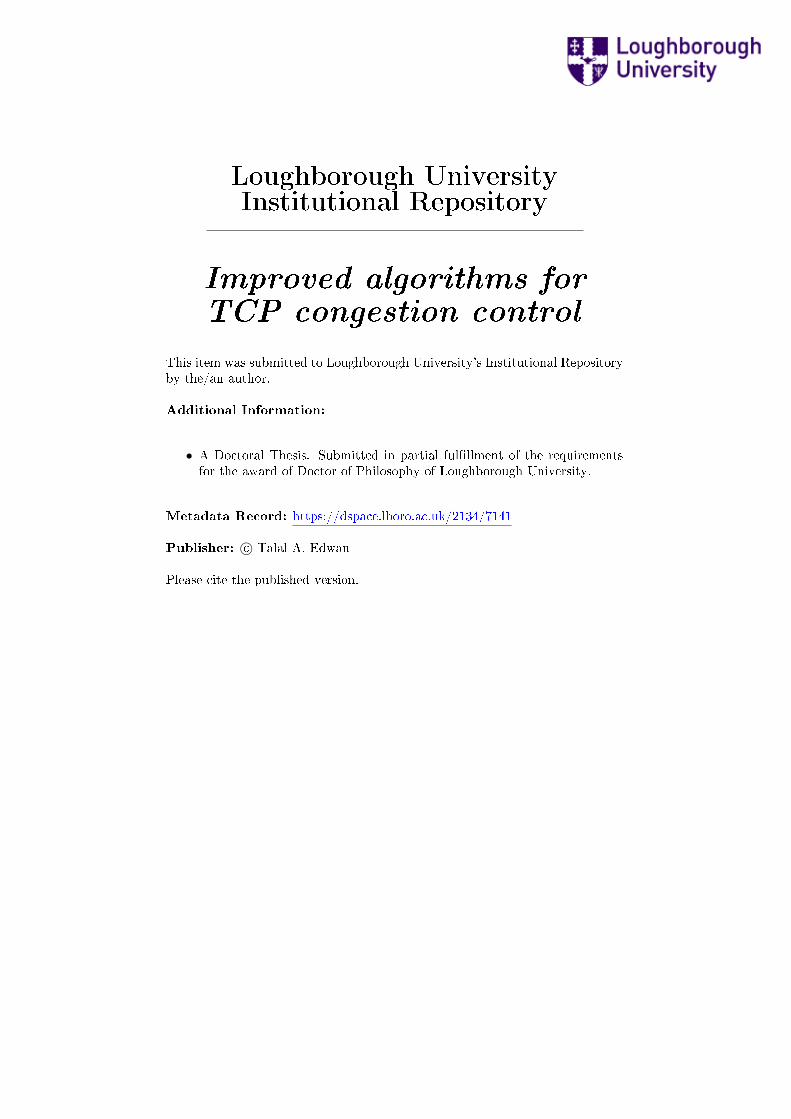
Table 2.1: TCP Throughput over LAN and WAN connections [51]
Network Type Nominal Bandwidth Actual TCP Throughput Achieved (%)
LAN 1.5 Mbps 0.70 Mbps 46.66WAN 1.35 Mbps 0.31 Mbps 22.96
Table 2.2: TCP Throughput over IEEE 802.11 connections [51]
Standard Nominal Bandwidth Actual TCP Throughput Achieved (%)
802.11 2 Mbps 0.98 Mbps 49802.11b 11 Mbps 4.3 Mbps 39.1
We focus our attention on the loss problem (which is due to high transmission
error rates) and how it affects TCP performance. Having mentioned that lower
layer error recovery cannot recover from all errors, this may lead to packets being
corrupted and thus discarded and not handed to TCP. TCP in turn makes a tacit
assumption that the lost packets are due to congestion and thus reacts by reducing
its congestion window drastically (multiplicative decrease). This results in an
unnecessary throughput reduction. We adopt some figures mainly for WLANs [51]
to show how severe the problem could be. Table 2.1 depicts TCP throughput over
a WLAN path and a WAN path consisting of a single WLAN plus 15 wired links.
The nominal bandwidth is the bandwidth in the absence of any losses, the actual
throughput is the throughput when the WLAN suffers from a frame error rate of
2.3% for a frame size of 1400 bytes. Table 2.2 shows the results for IEEE 802.11.
Note that high speed links are affected more since TCP drastically reduces its
throughput after each loss event (multiplicative decrease) and thus it takes longer
to reach the peak throughput supported by higher speeds [51]. Unnecessary TCP
throughput loss also occurs in cellular systems. In their voice mode the residual
frame error rate is 1-2% after low level error recovery. Another point to mention
here is that TCP works in the forward and reverse directions (data and ACKs), in
wireless links this could lead to undetected collisions which in turn increases the
frame error rate.
The SACK mechanism in TCP helps in recovering from multiple packet loss
quickly (i.e. in one round trip time), however, non-congestive packet loss is prob-
lematic for standard TCP CC because fast recovery is invoked and the congestion
window is halved.

CHAPTER 2. BACKGROUND 22
2.9 TCP & High-Speed Networks
2.9.1 Long Delay
The evolution of high-speed networks has facilitated the transfer of huge amounts
of scientific data like that gathered in Astronomy, Bioinformatics, Earth Sciences,
Physics etc. Nowadays, cross Atlantic data transfer between research institutes
is not uncommon. Such transfers need a reliable and efficient protocol that can
handle multiple simultaneous transfers and TCP is the most used reliable protocol.
TCP CC armed with its fixed AIMD mechanism may have a problem utilising
the full bandwidth of a high-speed long-delay pipe (this is usually referred to
as: high BDP). To see how TCP substantially underutilises network bandwidth
over high BDP connections; let us consider this case: suppose we have TCP flow
running over a 10 Gbps with RTT = 100ms, packet size = 1500 bytes = 12000
bits. This gives a BDP = 1010 × 0.1 = 109 bits, = 83, 333.33 packets. If TCP is
running in congestion avoidance phase, which means that the congestion window is
increasing by 1 packet each RTT, upon a packet loss event the window is halved.
So: ∆cwnd = (1/RTT )∆t, ∆t = ∆cwnd × RTT = 416666.67RTT = 4166.67
seconds = 1.16 hours to reach the peak i.e. full utilisation again. If packet size is
10000 bits, it takes ≈ 1.5 hours. In other words TCP needs a low packet loss rate
to achieve full utilisation and such low loss rates are not realistic especially with
the spread of new technologies like fibre optics and wireless networks, and even at
these low loss rates, it takes too long to fully utilise the link after a back off.
It has been shown [88, p.72], that TCP is not stable for large RTT. Another
way to look at this nonstability is by comparing the growth of the congestion
window for two flows, one with large RTT and another with small RTT. Recall
that the slope of a congestion window growth function over time is: α/RTT where
α = 1 for TCP. In fact, the flow with the large RTT (low slope) spends most of its
time increasing from the point at which packet loss happened to the peak, during
the same period; the flow with the small RTT (high slope) must have reached the
peak several times (reached steady state faster).8
2.9.2 Short Delay
The high-speed long-delay pipes are not the only potential problem for TCP. A
pathological behaviour of TCP in some high-speed low-delay environments has
been also identified. The problem can be seen when TCP works in a certain
communication pattern which is known as Incast. In this pattern a receiver issues
a request to multiple senders, the senders upon receiving the request concurrently
8This is my understanding.

CHAPTER 2. BACKGROUND 23
respond to the receiver. The sender traffic traverses a bottleneck link in a many-
to-one fashion and a potential for a congestion problem arise. In fact, a worst
case of congestion collapse can occur and the problem is usually referred to as
TCP-Incast.
Such communication pattern is not uncommon, it arises in typical data centre
applications: cluster-storage when data is stripped on multiple servers (for reli-
ability and better use of bandwidth) and servers need to respond to a request,
web-search when many workers respond to a search query. In these set-ups, the
data usually traverse an Ethernet switches which typically have small buffers of the
range 32KB-256KB; thus a high chance that they overflow in case of congestion.
Large companies (e.g. Google, Microsoft, Amazon, etc) use data centres for web
search, storage, e-commerce and large-scale computations. Thinking business; the
use of existing technologies is more cost effective, therefore the vast majority of
data centres use TCP for communication [23].
Technically (and historically) speaking, some of TCP parameters were tuned
for typical WAN environments, for example in Linux the intial retransmission
time-out timer is set (to a reasonable value for WAN) of 200ms, i.e. the sender
can make a decision of a time-out (lost packet) after 200ms. However, in an data
centre environment with low latency (or round trip time) this is considered long
and result in throughput degradation. To illustrate this point, suppose the sender
sends a number of packets (say a window) and they are all lost, then it will take
200ms to realise that they are lost and starts retransmitting. During this period
no packets are sent. Suppose that the retransmission time-out timer is close to the
round trip time i.e. a smaller value, then the sender will realise that the packets are
lost in nearly one round trip time and respond by retransmitting the lost packets,
thus we have more packets sent in the same period of time. It has been found that
using TCP with its current set-up and increasing the number of servers beyond
a certain number result in a huge drop in the receiver’s goodput9, this is due to
TCP large retransmission time-out value, window halving and time-outs.
One quick solution is to use large switch buffers. While this can delay the onset
of Incast, it comes at the price of substantial increase in the cost, e.g. switches
with 1MB packet buffering per port may cost $500,0000, TCP improvements e.g.
NewReno, SACK, RED, ECN, Limited Transmit and modification to slow start,
mitigate the problem but do not solve it. Ethernet flow control (when the sender
is sending too much traffic, the overwhelmed node can send a PAUSE frame to
throttle the sender) is effective when all nodes are on the same switch and less
effective when nodes are on different switches, this is due to inter-trunk head-of-
9Application-level throughput, we define this in chapter 5

CHAPTER 2. BACKGROUND 24
line blocking10
It has been shown that an effective solution is to reduce TCP’s retransmission
time-out to microsecond granularity, specifically; a value of 200µs achieves full
goodput for as many as 47 servers in real world cluster environment [7]. Deviating
from this point, their are other attempts to solve the problem at lower layers,
particularly the use of the so-called Quantised Congestion Notification(QCN) [82]
in Ethernet (see for example [4] for a modified QCN to alleviate the problem).
However we are not intending to elaborate on that in this thesis, our concern is
to focus on TCP solutions.
2.10 TCP-PEP Approach
One approach used to compensate for TCP performance degradation when work-
ing in different environments is the approach of TCP-Performance Enhancing
Proxies (TCP-PEP) [17, p.5]. In general, PEP can be integrated i.e. implemented
on a single node, or distributed i.e. implemented on multiple nodes. However, a
common mechanism used in TCP-PEP is to split11 a TCP connection into three
parts, where the first and last run standard TCP and another compensating proto-
col runs in the middle, this could be a different protocol e.g. XCP or an optimised
TCP algorithm e.g. high-speed long-delay TCP algorithm.
Three years ago12 an ISP used to have an asymmetric path (a shared E1 for
upload traffic and a higher bandwidth satellite link for download traffic) which
likely to make TCP perform badly! One such problem that may arise is ACK
compression at the upload link which results in undesirable bursts which in turn
are reflected as a bursts in the forward direction. Such bursts are not good for
the network. A TCP-PEP may be used to alter the ACK spacing to mitigate the
effect of bursts and thus smoothing TCP throughput.
Another example is the use of TCP-PEP to alter the behaviour of TCP con-
nection in a high BDP environment by generating local ACKs which make the
congestion window evolve faster (affects forward performance) and thus enhance
throughput. As said in the first paragraph of this section, this can be accompa-
nied by another protocol/algorithm which takes the responsibility of sending the
data over a high BDP pipe. There are other examples, like the use in VSAT and
10In a cross-bar switch fabric, when two ports have packets in their input queues destined tosame output port, a contention may appear; which blocks the rest of packets in a FIFO inputqueue.
11Some may argue if this breaks the end-to-end argument [83] i.e. functionality is restricted atend-hosts. There is no functionality replacement at end hosts, PEPs adds performance optimi-sation to a subpath of the end-to-end path and that agrees with the end-to-end argument [17].
12This is based on the author’s experience.
CHAPTER 2. BACKGROUND 25
WLAN environments. A typical example of the use of TCP-PEP in WLAN is
TCP-Snoop [10], this is briefly discussed in chapter 3.
We end this section with a science fiction note. In 1781 Sir William Herschel
announced the discovery of Uranus (the seventh planet from the Sun). Later on,
in 1986 the spacecraft Voyager-2 (unmanned interplanetary space probe) reached
Uranus, four days before that scientists noticed jittered sent images caused by a
software bug. The software bug was resolved and a piece of code was sent over
3.2 × 10⁹km to Voyager-2 at the speed of light (300 × 103km/s) in three hours.
The problem was solved and clear images were received.
Indeed there is no need to use a protocol with congestion control for the case
in the previous paragraph, but we build an imaginary case based on it, it might
appear in one of science fiction movies and may become true one day. The case
is: having a multiple nodes (probes) in space, where these nodes are supposed to
capture some scientific data and send it back to the Earth. Depending on the size
of data and the number of nodes and the capacity of links and the hardware used
in future, a congestion control problem may appear. If TCP is still used by that
time, TCP-PEP may be considered as a solution. Since for example based on the
previous paragraph, a round trip time of six hours may not fit a congestion control
algorithm, for instance, one choice is to split a connection (multiple connections)
and run a space version (e.g. aggressive rate increase) of TCP in the middle.
Alternatively, in literature we found three ways (at network layer) for packet
networks to deal with congestion [94]: i) Warning bit (ECN is an example), ii)
Choke packets, iii) Hop-by-hop choke packets. The hop-by-hop choke packets can
also be considered as another choice to mitigate the previous problem.
2.11 Explicit Feedback Issues
TCP follows an end-to-end approach and treats the network as a black box, how-
ever the network can play an explicit role in mitigating the congestion problem.
In this section we look at two examples13 which we believe are related in the con-
text14 of TCP CC. The first one is Explicit Congestion Notification (ECN) [81]
appeared in 2001 and the second one is Quick-Start mechanism [35] appeared in
2007.
ECN assumes that the network has some sort of Active Queue Management
13A third example is ICMP source Quench message sent back to the sender to reduce the ratein case of congestion. This technique is rarely used in the Internet: consumes bandwidth, dueto being ineffective and unfair [45]
14There are network assisted protocols which need special routers, these are believed to bealternatives to TCP CC, an example is Explicit Control Protocol XCP [57] , these are notdiscussed in this thesis.
CHAPTER 2. BACKGROUND 26
(AQM) which usually detects congestion proactively through (for example) aver-
age queueing delay, and reports this as a binary (congestion,no congestion) feed-
back information in the packets. There is no point in reporting this if the senders
are not cooperating by changing their rates, thus ECN requires support from trans-
port layer protocol(s). Information about ECN-Capability and binary feedback
information can be conveyed via four code points i.e. two bits in the IP header
of a packet, where two code points indicate if the transport protocol is capable of
using the ECN information e.g. has headers to send congestion information to the
other end, these two code points are called: ECN-Capable Transport (ECT). The
other two code points are: non-ECT and Congestion Experienced (CE).
TCP cooperates with ECN by dedicating two flags in its header: ECN-Echo
(ECE) by which the receiver can inform the sender when a CE packet has been
received and a Congestion Window Reduced (CWR) by which the sender can
inform the receiver that it responded by reducing the rate. Typically the ECN-
Capability of TCP is negotiated during the connection set-up and the ECT is
set.
A typical sequence of events is that a queue threshold is exceeded, congestion
experienced bit(s) in the IP header field are set. In response to that when an
ECN-Capable TCP receiver receives this information it echos it back by setting
ECE in an ACK packet, the sender then backoffs exactly as it does when a packet
drop happens and inform the reviver about this by setting the CWR in a forward
packet. The approach reduces delay by preventing buffer overflow and reduces
packet drop rates (if marking is used).
Another example of network cooperation, is Quick-Start which tries to find
the appropriate initial congestion window size (and thus the available bandwidth)
quickly i.e. in one round trip time. Opposed to Slow-Start available bandwidth
probing mechanism, Quick-Start suggests an explicit feedback from all the routers
along the path, for instance; the TCP sender would set its desired rate in bytes per
seconds in a Quick-Start option in the IP header of a packet. Each router along
the path can the either: i) Approve the requested rate, ii) Reduce the requested
rate, iii) Unapprove the requested rate. The TCP receiver communicates this
information back the the sender in an answering packet and the rate (congestion
window) is adjusted accordingly. Subsequent transmissions are then governed
by the congestion control algorithm. However if the request is not approved the
default congestion control algorithm is used. An interesting point is that the range
of the requested rate is: 80 Kbps - 1.3 Gbps. Which means that TCP CC can
significantly benefit from this technique when working in a high speed long delay
environments.

CHAPTER 2. BACKGROUND 27
2.12 Summary
In this chapter we discussed a number of definitions of congestion control problem.
We discussed the difference between terms like “congestion avoidance” and “con-
gestion control” and how the goal of congestion control changes in time. First it
was to prevent congestion, and nowadays to efficiently utilise high capacity links.
We focused on end-to-end solutions and because these solutions rely on adapting
the source rate, we discussed a number of approaches used to adapt the source
rate, we classified these into three classes: i) Linear algorithms, i) Non-linear al-
gorithms, iii) Equation-based algorithms. Then we looked at the practical side of
some of these solutions, mainly the most deployed protocol, TCP, then Multipath
TCP. We steered the discussion towards some challenges to TCP in high-speed
low-latency networks (e.g. TCP Incast), high-speed long-delay networks and wire-
less networks, this is followed by a general approach (TCP-PEP) that can be used
to mitigate some of these problems. Finally, we mentioned that TCP can coop-
erate with other approaches which gather information from network, we provided
two examples: i) ECN as an explicit congestion notification, ii) Quick-Start mech-
anism to determine the initial window size. However, solutions for the challenges
that we left open are discussed in the next chapter with more elaboration.

Chapter 3
TCP Congestion Control Variants
This chapter sheds the light on a number of TCP congestion control algorithms
aimed at optimising the performance of TCP in high-speed long-delay networks,
it also mentions other variants designed to enhance the performance of TCP in
different set-ups e.g. wireless networks. The chapter is divided as follows: in
section 3.1 we briefly discuss a number of high-speed long-delay TCP variants, we
used the notation: TCP-X, (where X is the name of that variant) to refer to the
variant under discussion in each subsection. We elaborate more on TCP-Illinois
and TCP-YeAH variants in chapter 6 and chapter 7 respectively. In section 3.2
we mention a number of other TCP variants. Finally we summarise in section 3.3
the ideas in this chapter.
3.1 TCP for High-Speed Long-Delay Networks
In the last decade, the research community responded with a number of congestion
control algorithms aimed to moderate the problem of bandwidth under-utilisation
of high BDP pipes [69, 102, 47, 32, 61, 64, 27, 93, 9], we visualise some of these
in figure 3.1 and provide a briefing of some of them in this section.
We have noticed that a common thing between all these algorithms is that
their designs are influenced by the following points:
• Scalability or utilisation, efficient use of bottleneck link.
• RTT fairness
• TCP friendliness, backward compatibility with TCP when deployed in low-
speed short-distance networks.
• Fairness, equal number of packets in flight at each congestion event.
28

CHAPTER 3. TCP CONGESTION CONTROL VARIANTS 29
FASTTCP−
WestwoodTCP−
CompoundTCP−
TCP− ?
TCP− ?
Westwood+Hamilton
STCP
TCP−Reno
TCP−Africa
TCP−Illinois
TCP−BICTCP−CUBIC
TCP−HS TCP−
TCP−Vegas
TCP−TCP−Hybla
TCP−Veno
TCP−YeAH
Figure 3.1: A number of TCP congestion control stacks
• Responsiveness in terms of convergence, respond quickly to changes in avail-
able bandwidth.
We also found that a simple way to characterise an algorithm and reveal many
of these points is by using the so-called Response Function, this is basically the
average throughput as a function of the back off probability (just to link ideas, this
is the same equation that we mentioned in chapter 2, when we discussed equation-
based algorithms, some refer to it as throughput equation). Some information can
be directly revealed from a response function:
• Scalability
• RTT fairness
• TCP friendliness
The well-known expression of TCP-Reno in steady state average rate for small
packet loss rates was found to be:
X ∝ 1
RTT
√1
βp
A closed form was derived [78], we mention the simplified result here:
XTCP ≈1
RTT
√3
2bp

CHAPTER 3. TCP CONGESTION CONTROL VARIANTS 30
And for a deterministic AIMD decrease model [36]:
XAIMD ≈1
RTT
√
α(2− β)
2βp
For a stochastic model [103] and also mentioned in other literature [47]:
XAIMD ≈1
RTT
√
α(1 + β)
2b(1− β)p
Where, α and β are constants, b is the number of packets acknowledged by
each ACK (in normal operation b = 1, for delayed acknowledgement b = 2). Note
that β = 1/2 here.
The deterministic AIMD model assumes that a packet is dropped each time
the congestion window reaches a certain fixed number of packets. In contrast, an
AIMD stochastic model assumes that packet is dropped randomly [36]. In fact this
is the AIMD model mentioned in [103]. The advantage of the deterministic model
is its simplicity and usefulness for focusing on the role of the α and β in AIMD
congestion control, however the stochastic model gives more accurate model under
certain assumptions.
If the response function has the form: c/pd where, c and d are constants then
by taking a log scale (i.e. the slope becomes the absolute value of d), the following
properties can be deduced:
• As d increases the slope of the function increases and the scalability of the
algorithm increases (i.e. large windows at low loss rates).
• RTT unfairness is roughly proportional to (RTT2/RTT1)d/(1−d), so if d in-
creases the slope of the function increases and the RTT unfairness increases [102].
• TCP friendliness can be seen from the point where the response function of
an algorithm crosses that of standard TCP. If it crosses TCP at lower loss
rates then its more TCP friendly. The reasoning behind that ([102]) is since
TCP does not consume too much bandwidth at low loss rates (remember,
this is the problem with the TCP algorithm) other algorithms could apply
their scalable techniques and consume what is left from TCP, so here we
say, they are not working like TCP in this region. After this point (i.e. the
crossing point) they start working like TCP. In other words it becomes more
TCP friendly if an algorithm function crosses TCP’s function as low as loss
rate as possible.
We recreated a response function plot of a number of TCP variants. Figure 3.2
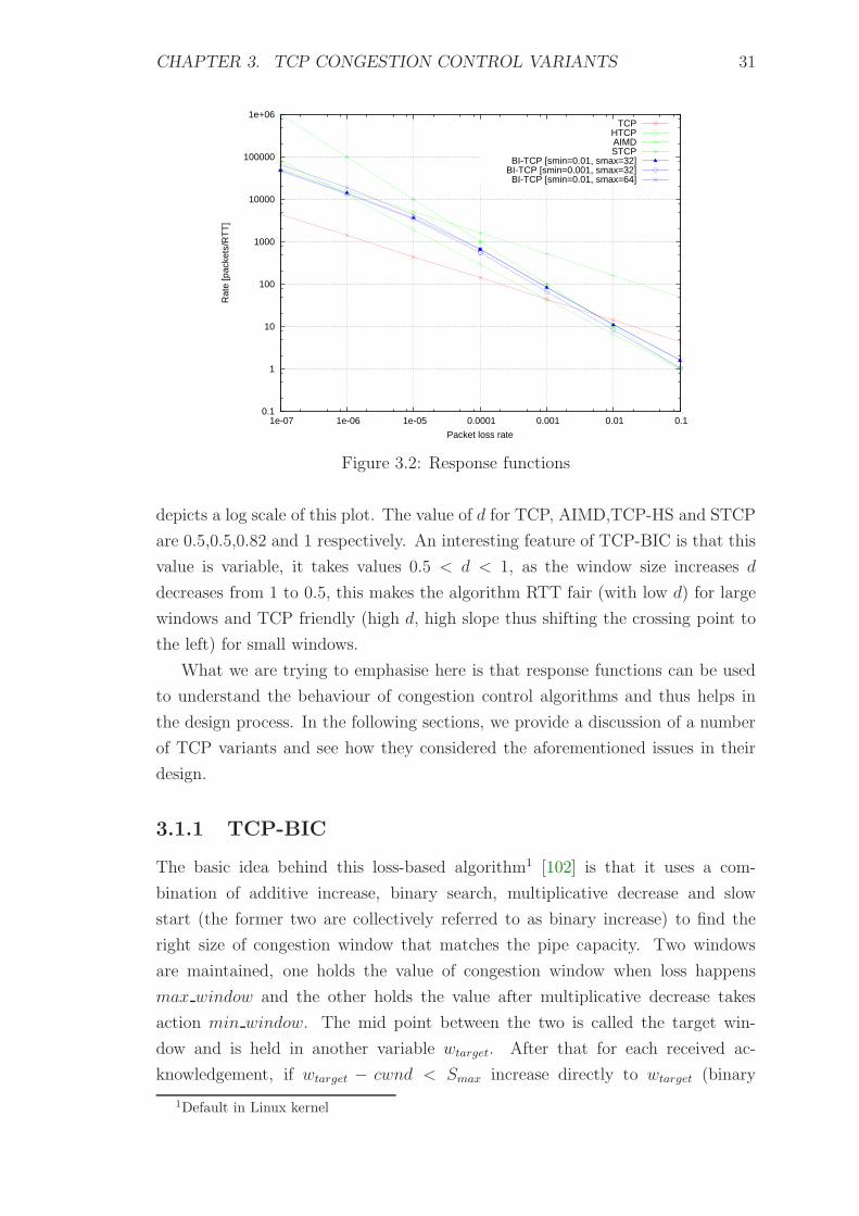
CHAPTER 3. TCP CONGESTION CONTROL VARIANTS 31
0.1
1
10
100
1000
10000
100000
1e+06
1e-07 1e-06 1e-05 0.0001 0.001 0.01 0.1
Rat
e [p
acke
ts/R
TT
]
Packet loss rate
TCPHTCPAIMDSTCP
BI-TCP [smin=0.01, smax=32]BI-TCP [smin=0.001, smax=32]
BI-TCP [smin=0.01, smax=64]
Figure 3.2: Response functions
depicts a log scale of this plot. The value of d for TCP, AIMD,TCP-HS and STCP
are 0.5,0.5,0.82 and 1 respectively. An interesting feature of TCP-BIC is that this
value is variable, it takes values 0.5 < d < 1, as the window size increases d
decreases from 1 to 0.5, this makes the algorithm RTT fair (with low d) for large
windows and TCP friendly (high d, high slope thus shifting the crossing point to
the left) for small windows.
What we are trying to emphasise here is that response functions can be used
to understand the behaviour of congestion control algorithms and thus helps in
the design process. In the following sections, we provide a discussion of a number
of TCP variants and see how they considered the aforementioned issues in their
design.
3.1.1 TCP-BIC
The basic idea behind this loss-based algorithm1 [102] is that it uses a com-
bination of additive increase, binary search, multiplicative decrease and slow
start (the former two are collectively referred to as binary increase) to find the
right size of congestion window that matches the pipe capacity. Two windows
are maintained, one holds the value of congestion window when loss happens
max window and the other holds the value after multiplicative decrease takes
action min window. The mid point between the two is called the target win-
dow and is held in another variable wtarget. After that for each received ac-
knowledgement, if wtarget − cwnd < Smax increase directly to wtarget (binary
1Default in Linux kernel

CHAPTER 3. TCP CONGESTION CONTROL VARIANTS 32
search) otherwise increase by Smax (additive increase2), update the following:
min window = cwnd,wtarget = max window+min window2
. Perform slow start any
time the current window grows past max window (since the maximum window is
unknown the above sequence is effective-less, so probing for max window stars). To
aid convergence, the algorithm use a Fast Convergence technique that exploits the
down trend of congestion window when another flow starts competing for band-
width. The previous max window is memorized in prev window and when loss
happens, if prev window > max window the algorithm computes the mid value
but this time it sets the max window to this value then computes a mid value
again (based on the new maximum window) and sets the wtarget to this value. To
achieve TCP friendliness, the algorithm operates like standard TCP if the conges-
tion window is below certain threshold. Figure 3.3 depicts the congestion window
evolution of the two flows using the algorithm and competing for bottleneck link
using a Drop-Tail queue.
Figure 3.3: Congestion windows: two TCP-BIC flows competing for band-width [102]
3.1.2 TCP-CUBIC
This algorithm [47] is an improvement over TCP-BIC, it tries to achieve the same
congestion window evolution of TCP-BIC while making it less dependent on round
trip time in an attempt to achieve RTT-fairness between flows. The idea is to
adapt the congestion window in real time according to a function. The function
is shown below, t is the elapsed time since last back off
cwnd =
{
cwndtcp = cwndmaxβ + 31−β1+β
tRTT
if cwndtcp > cwndcubic
cwndcubic = C(t−K)3 + cwndmax otherwise
2Binary search and additive increase are collectively referred to as: binary increase

CHAPTER 3. TCP CONGESTION CONTROL VARIANTS 33
If cwndtcp is larger than the cwndcubic this means that the the algorithm is likely
to be working in a short round trip time network, therefore the TCP window is
selected, however if cwndcubic is larger, then the algorithm likely to be working
in a long round trip time network and the CUBIC window is selected. Recent
studies [91] have shown that the algorithm causes collateral damage to real-time
traffic on broadband networks.
3.1.3 TCP-Illinois
As it can be seen from figure 3.3, the concavity feature of congestion window is
desirable, this actually leads to larger area under the curve which translates to
more packets being transmitted. Another loss-delay based algorithm with this fea-
ture is TCP-Illinois [69]. The algorithm uses additive increase and multiplicative
decrease (upon loss):
Ack : cwnd ← cwnd + fα(da)cwnd
Loss : cwnd ← (1− fβ(da))× cwnd
But it adapts the AI and MD parameters according to estimated average queueing
delay, fα(da) ∝ 1da
and fβ(da) ∝ da. The basic idea is to estimate the maximum
average queueing delay as the difference between the maximum and minimum
average round trip times seen so far by the flow during a connection. Then to
estimate the current average queueing delay (estimation is done each round trip
time i.e. each time a window is sent). If the estimated average queueing delay is
close to the estimated maximum delay then it sets small AI and large MD, if the
it is far it sets large AI and small MD. The algorithm falls back to standard TCP
operation if the congestion window is below a threshold. One advantage of this
algorithm is that, adapting the MD parameter in this way increases the immunity
against non-congestive packet loss, a disadvantage; however, is that a receiver can
cheat by increasing the round trip time, thus the sender thinks that there is a large
queue and overestimates the maximum round trip time, subsequently the current
average delay is likely to be far from the maximum delay and the AI is large. We
address other issues of this algorithm and propose solutions in chapter 6.
3.1.4 TCP-HS
Another algorithm that uses AIMD is TCP-HS [32], the algorithm adapts AI and
MD as a functions of the congestion window size.
Ack : cwnd ← cwnd + fα(cwnd)cwnd
Loss : cwnd ← fβ(cwnd)× cwnd

CHAPTER 3. TCP CONGESTION CONTROL VARIANTS 34
Where, fα(.) ↑ and fβ(.) ↓ as cwnd ↑. Again, the algorithm engages after a window
threshold. The idea is to adjust α and β so that the response function gives certain
W/RTT at certain high p(W ) (low window), and higher W1/RTT at certain low
p(W1) (high window).
3.1.5 STCP
Scalable TCP [61] algorithm adopts a multiplicative increase and multiplicative
decrease approach, while this is very scalable it has fairness and RTT unfairness
issues, however the rule is simple simple to implement and scalable for high-speed
long-delay networks,
Ack : cwnd ← cwnd + α
Loss : cwnd ← β × cwnd
Where, α = 0.01, β = 0.875 and the algorithm engages after a window threshold.
3.1.6 TCP-Hamilton
This algorithm updates the congestion window as a function of elapsed time since
last congestion event, the function was chosen to achieve a response function
similar to that of TCP-HS.
Ack : cwnd ← cwnd + 2(1−β)fα(∆)cwnd
Loss : cwnd ← fβ(B)× cwnd
fα(∆) =
{
1 if ∆ ≤ ∆L
max(fα(∆) ∗ Tmin, 1) if ∆ > ∆L
fβ(B) =
{
0.5 if |B(k+1)−B(k)B(k)
| > ∆B
min( Tmin
Tmax, 0.8) otherwise
Where, ∆ is the elapsed time since the last congestion event, ∆B = 0.2, B(k+1) is
the maximum achieved throughput during the last congestion epoch and: fα(∆) =
1 + 10(∆−∆L) + (∆−∆L
2)2
3.1.7 TCP-FAST
This algorithm [54] is a delay-based algorithm, it adapt the AI parameter according
to a predefined function based on the congestion window and average queueing
delay. The congestion window is updated as a smooth average:
Every RTT : cwnd ← (1− γ)(cwnd) + γ(
Tmin
Tcwnd + fα(cwnd, da)
)
Loss : cwnd ← β × cwnd

CHAPTER 3. TCP CONGESTION CONTROL VARIANTS 35
Where, β = 0.5, Tmin and T are minimum and average observed round trip times
respectively, da is the average queueing delay. The algorithm also reacts to loss
by multiplicatively decreasing the congestion window. Note that the congestion
window update rule has a component that is inversely proportional to the average
round trip time i.e. it decreases every round trip time (gradually) as the queue
builds up (congestion), rather than waiting for packet loss to happen, in other
words this is a CA rather than a CC approach (to link ideas, please see figure 2.2).
3.1.8 TCP-YeAH
Yet Another High speed algorithm [9], tries to exploit the network bandwidth
efficiently while putting less stress on the network compared to standard TCP.
The basic idea is to have two different modes of operation: Fast and Slow modes.
In the fast mode the congestion window is incremented according to an aggressive
rule (STCP rule was used for ease of implementation but any other rule can be
used). In the slow mode the congestion window is incremented like standard TCP
and a precautionary decongestion algorithm is implemented.
Switching between slow and fast modes is decided according to the estimated
number of packets in the bottleneck queue. This number is estimated as follows [9]:
Let RTTbase be the minimum RTT measured by the sender (estimate of propaga-
tion delay) and RTTmin the minimum RTT estimate in the current data window
of cwnd packets and thus is updated once per window of data (i.e. each RTT). The
current queuing delay can be estimated as RTTqueue = RTTmin − RTTbase. This
RTTqueue is then used to infer the number of packets enqueued at the bottleneck
as:
Q = RTTqueue.G = RTTqueue.
(cwnd
RTTmin
)
Where, G is the goodput. The ratio3 between the queuing delay and the propa-
gation delay L = RTTqueue/RTTbase is used to indicate network congestion level.
If Q < Qmax and L < 1/ϕ, the algorithm is in the fast mode, otherwise it is in
the slow mode. Qmax and ϕ are tunable parameters; Qmax is the maximum number
of packets a single flow is allowed to keep into the buffers. 1/ϕ is the maximum
level of buffer congestion with respect to BDP. The precautionary decongestion
algorithm is to diminish the congestion window by Q whenever Q > Qmax and the
to set the slow start threshold to half the congestion window.
The fact that the queue estimate keeps exceeding Qmax even after applying
the decongestion algorithm is logically coupled with the fact that there is a greedy
competing source and this is the rational for falling back to slow mode. In other
3This can be thought of as the ratio between the number of packets enqueued and the pipe’sBDP

CHAPTER 3. TCP CONGESTION CONTROL VARIANTS 36
words if TCP-YeAH spends more time in the slow mode that it does in the fast
mode then it is more likely that it is competing with a greedy source. However
TCP-YeAH does not continue this polite behaviour of diminishing its congestion
window by Q when competing with greedy sources. It maintains count (this count
in fact represents an estimate of the competing standard TCP congestion window,
since it increase by one packet each RTT), the count is incremented each time
the algorithm finds itself in the slow mode. If the congestion window reaches
this count or less, it stops decreasing for not to let the window drop below the
estimated standard TCP window, then it starts increasing increasing like standard
TCP. When packet loss happens the count is halved.
One point to note here is that the queue estimate (Q) is done each RTT, i.e.
this is the granularity of decongestion, thus considering flows with different RTTs,
each flow reaches Qmax at different time and thus diminish its excess packets in
the queue at different time without affecting link utilisation. Therefore, in theory
the algorithm achieves RTT fairness. In chapter 7 we proposed an increase rule
for this algorithm which automatically assigns small increase for flows with small
RTT and large increase for flows with large RTT, thus improving RTT fairness.
3.1.9 TCP-Compound
This algorithm [93]4 is a loss-delay based algorithm, it maintains a compound con-
gestion window: loss-based congestion window and delay-based congestion win-
dow, so TCP’s window becomes: min{cwnd + dwnd, awnd}. The basic idea is
to use an aggressive binomial rule (to link ideas please see figure 2.5, IIAD as an
example) in the delay-based congestion window, after reaching a certain number
of packets determined by a threshold γ, the delay-based congestion window dimin-
ishes by ζdiff 5. The loss-based congestion window increases normally according
to standard TCP rule. However note that even after reaching the threshold and
the delay-based congestion window decreases, there are still packets in the queue
due to the loss-based congestion window, as a result the delay-based congestion
window keeps decreasing until it disappears, effectively leaving only the loss-based
congestion window. The overall congestion window evolves according to the fol-
lowing rules [93]:
Ack : cwnd ← cwnd + αcwnd+dwnd
Loss : cwnd ← (1− β) ∗ (cwnd + dwnd)
4Default in Windows XP and Vista SP1. Discontinued in Linux kernel code base since 2.6.175Note how this component is similar to what was mentioned about TCP-YeAH

CHAPTER 3. TCP CONGESTION CONTROL VARIANTS 37
dwnd← dwnd + α((cwnd + dwnd)k − 1)+ if diff < γ
dwnd← dwnd− ζdiff if diff ≥ γ
dwnd← ((cwnd + dwnd)(1− β)− cwnd2
)+ if Loss/ECN
diff is the estimated number of backlogged packets:
Expected = cwnd+dwndbaseRTT
Actual = cwnd+dwndRTT
diff = (Expected − Actual) ∗ baseRTT
The parameters were selected so that the algorithms gives a response function
similar to that of TCP-HS (i.e. by comparing both response functions). They are
found to be: k = 0.8, α = 0.125, β = 0.5, for implementation purposes k was set
to 0.75. (easier through the use of fast integer algorithm of square-root). An auto-
tuning algorithm (gamma auto-tuning) was proposed for empirically adjusting the
γ value.
3.2 Other TCP Variants
There are so many TCP variants customised to achieve different goals, in this
section we only mention some which are related in the context of this thesis.
One of the earliest proposals was TCP-Vegas [19] which is totally a delay-based
algorithm, the idea is very similar to that of the algorithm ([98]) mentioned in
chapter 2. TCP-Vegas algorithm calculates the difference between actual rate
and expected rate and if this is less than a threshold (α) it increases linearly, if
the difference is larger that another threshold(β) it decreases linearly and if the
difference is larger than α and less than β then the congestion window remains
unchanged. The algorithm achieves better throughput compared to standard TCP,
however, the additive decrease nature makes it less responsive and rise fairness
issues.
A hybrid algorithm which combines features from standard TCP (Reno) and
TCP-Vegas is TCP Veno [44], the algorithm estimates the number of backlogged
packets at the bottleneck using TCP-Vegas parameters(N = Actual ∗ (RTT −baseRTT )), if this number is less than a threshold (β) a non-congestion state is
assumed and the increase rule of standard TCP is adopted but the multiplicative
decrease parameter is set to a high value (4/5). However, if the number is greater
than or equal the threshold, a congestion state is assumed and the congestion
window is increased by one packet every other round trip time instead of one
packet every round trip time (i.e. less aggressive and more concave window) and
the multiplicative decrease parameter is set to 1/2.

CHAPTER 3. TCP CONGESTION CONTROL VARIANTS 38
TCP-Westwood [20] alters the congestion window upon congestion i.e. when
receiving duplicate ACK or time-out. The idea is measure the flow rate by mon-
itoring and filtering the rate of ACK at the source. By doing so, the congestion
window can be deduced by multiplying the rate by the minimum round trip time
RTTmin, the slow start threshold and the congestion window are then set to this
values (instead of halving the window). In case of time out, only the slow start
threshold is set to this value and the congestion window is to 1 packet. All other
increase rules of standard TCP are maintained. An advantage of this approach
is that it is immune against non-congestive packet loss, particularly; due to the
increase rules of the algorithm, it fits wireless environments.
Finally, TCP-Snoop [10] tries to confine packet retransmissions over the wire-
less link of the path only by snooping inside TCP connections and transparently
transmit corrupted packets. The basic idea is to run a snoop agent at wireless gate-
way, the agent maintains a state for each flow traversing the gateway and packets
sent from the wired host (sender) to the wireless host (receiver) are cached lo-
cally. If duplicate ACKS are received the agent perform local retransmission and
suppress the duplicate ACKS, thus prevents the sender from doing retransmission
and invoking congestion control algorithm(s). It has been mentioned that if the
direction of flow is reversed i.e. the sender on the wireless side, acknowledgements
may take long time and this may have impact on performance [51]
3.3 Summary
In this chapter we discussed a number of TCP congestion control proposals that
are mainly optimised to overcome the high-speed long-delay problem. Their are
a number of important factors in the design of such proposals: efficiency, RTT
fairness, TCP friendliness, fairness and responsiveness. We also showed that lots
of these factors can be inferred directly from a response function plot.
We found that the proposals are either loss-based (reactive approach, CC)
or delay-based (proactive approach, CA), or hybrid approach (CC,CA). They are
trying to achieve similar goals but in different ways, however they are experimental
and operating systems have different default algorithms. In fact some default
proposal in certain operating systems are discontinued in other operating systems.
Recent studies showed that some of these algorithms have adverse effects on real
time traffic.
We showed examples of other TCP congestion control proposals that try to
solve other problems, for example flatten and increase the throughput, increase
the immunity against non-congestive packet loss and thus increase the throughput.

Chapter 4
Optimisation & Congestion
Control
It is valuable to understand the formulation of congestion control problem as a
resource allocation problem, before actually tackling any of the problems men-
tioned in the previous chapters. For this reason we provide a discussion of this
formulation and some stability issues related to TCP congestion control.
This chapter is structured as follows: in section 4.1 we discuss the formulation
of congestion control problem as a resource allocation problem. Section 4.2 high-
lights a three different types of algorithms that can be used to solve the resource
allocation problem, we finalise this section by relating this to TCP congestion
control. In section 4.3 we contribute and extend the current work by analysing a
non-linear case with non-congestive packet loss and a version of TCP with a vari-
able MD. We further explore the dynamics of TCP in section 4.4 by linearising
the model around an equilibrium point. Finally we conclude in section 4.5.
4.1 Congestion Phenomenon & Resource
Allocation
In this section we discuss the formulation of congestion control problem as a
resource allocation problem, the intention is to give the reader a general idea
about how the problem is formulated and how stability techniques can be applied,
without going into details. A simple case of single link single source was used
in all cases. However the extension to multiple sources and multiple links can
be done using algebraic techniques (e.g. matrices etc ). In fact a comprehensive
analysis has been done on that in literature [88]. In spite of that we analysed some
special/hypothetical cases which up to our knowledge have not been analysed in
the same context.
39

CHAPTER 4. OPTIMISATION & CONGESTION CONTROL 40
4.1.1 Resource Allocation
The resource allocation problem is that of fairly assigning rates to users who share
a common link. In this case the resource is the capacity of the link. Note that this
semantic also agrees with the congestion control (using the network efficiently).
However this problem can be viewed as an optimisation problem [88] this is ba-
sically to maximise or minimise a function subject to fixed outside conditions or
constraints. The method of Lagrange multipliers is usually used for solving this
class of problems. An example of this type of problems is: How can we minimise
the aluminium used to make a “can” while making sure it can hold 100 ml of
liquid?
In general, if f(x) is a differentiable concave function, and H is a matrix of
appropriate dimension (could be constant), then the problem can be formulated
as:
maxx
f(x), (4.1)
Subject to:
Hx ≤ c
f(x)optimal point
gradient vector
Figure 4.1: Graphical illustration of the Lagrange multiplier method.
Where c is the constraint. Figure 4.1 illustrates the graphical inspiration of the
problem. Note that at the optimal point the gradient vectors (normal to the curve
/ surface / . . . ) are in the same direction but could have different magnitudes. We
could equate both gradient to find the optimal point. However a more formal way
is to define a function then differentiate it and equate it to zero. This function is
usually referred to as the Lagrangian function. The Lagrangian function L can be
written as:
L(x, λ) = f(x)− λT (Hx− c),∂L∂x = 0, =⇒ ▽f(x)−HTλ = 0.
(4.2)
And,

CHAPTER 4. OPTIMISATION & CONGESTION CONTROL 41
λT (Hx− c) = 0. (4.3)
Where λ ≥ 0 is the Lagrange multiplier. And▽f(x) = (∂f/∂x1, ∂f/∂x2, . . . , ∂f/∂xn)
is the gradient vector. If x satisfies 4.2 and 4.3, then it solves 4.1.
Another formal way to look at the problem is through the so-called duality [88].
This is basically putting the function of our interest in another way. This can be
done by fixing the the Lagrangian function at a certain point of x and varying the
multiplier λ to reach the optimal value (instead of fixing ~λ and varying x in first
method, which is also called the primal method). Obviously λ should be tuned to
find the minimum of the new function (which is now a function of the multiplier
only). To illustrate this point we will write the new function which is called the
dual function [88], as:
D(~λ) = maxx∈C
L(x, ~λ) (4.4)
Where C is the set of all x. We can also write:
f(x) ≤ f(x)−~λT (Hx− c)︸ ︷︷ ︸
≥0
maxx∈C f(x) ≤ maxx∈C{f(x)− ~λT (Hx− c)} = D(~λ)
f(x) ≤ min~λ≥0 D(~λ).
For concave objective function and linear constraints, the equality of the above
equation holds, which means that the primal and dual objectives are the same.
Figure 4.2, depicts a graphical interpretation of the primal and dual methods.
Both solves 4.1 but from different perspectives.
L(x, λ )
max{L(x, )}λD ( λ ) =
f( x )
x x
λ
λ x
x
f( x )
{ x }
( b )( a )
Figure 4.2: Optimal objectives: (a) Primal method (b) Dual method.
To relate this to the resource allocation problem, we will adopt the approach
mentioned in [88] and assume we have r users sharing a route from a source to
a destination. Each user has a rate xr bps, and drives a utility function Ur(xr).

CHAPTER 4. OPTIMISATION & CONGESTION CONTROL 42
Then the optimisation problem is:
max{xr}∈S
∑
r
Ur(xr) (4.5)
With the constraints of:∑
r:ℓ∈r
xr ≤ cℓ, ℓ ∈ L, (4.6)
xr ≥ 0, r ∈ S,
Where:
cℓ: is the capacity of the link;
L: is the set of all links in the route;
S: is the set of all sources in the network;
Ur(xr): for each r, is a contiguously differentiable, non-decreasing, strictly concave
function, and for all r, Ur(xr)→ −∞ as xr → 01.
Depending on the type of the utility function, we define the following types of
fairness:
1. Weighted proportional fairness: when Ur(xr) = wr log xr, and because of the
property of convex functions the following holds:∑
r∈S U ′r(xr)(xr− xr) ≤ 0,
thus∑
r∈S wrxr−xr
xr≤ 0. Were xr is the optimal user rate. To illustrate this
property of convex functions we do the following: if we take the first order
Taylor series expansion of a convex function f(y) at point x, this gives
f(x) + (y− x)f ′(x), where f ′(.) is first derivative. This is an approximation
of the function around the point x and the equation is a line equation. If the
function is convex, any point on this line is less or equal than any point on
the actual function, i.e. f(x) + (y − x)f ′(x) ≤ f(y). A special case appears
when y = x, since f(x) ≤ f(x) we get: (x− x)f ′(x) ≤ f(x)− f(x) ≤ 02
2. Minimum potential delay fairness: when user with rate xr attempts to trans-
fer a file of size wr, the requires transfer time is wr/xr, let Ur(xr) = −wr/xr,
note that the minus sign is to make the function concave, in this context
we say that the problem is to maximise the sum of the utility functions and
we take the absolute value of the final result. This is equivalent of taking a
convex function Ur(xr) = wr/xr and minimising the sum of utility functions.
Both cases have the same meaning of minimising the total file transfer time.
3. Max-Min fairness: Here the capacity of the link is divide among the users in
such a way that the only way to increase a user rate is to decrease the rate
1We will see later that this does not hold for TCP congestion control algorithm2We add this illustration for sake of clarity.

CHAPTER 4. OPTIMISATION & CONGESTION CONTROL 43
allocated to some other source. It can also be shown that the users rates
allocation is max-min fair if and only if every user has a bottleneck [88]. In
the case of single bottleneck in the network, this implies an equal share of
the resource among the user flows through it [60]. An approximate utility
function for this case could be: Ur(xr) ≈ 1/(αxrα) for large values of α
A general class of utility function mentioned in [88] is:
Ur(xr) =
{
−wrx1−αr
1−αr, αr > 0, αr 6= 1
wr log xr, αr = 1(4.7)
Where:
Proportional fairness −→ αr = 1, ∀rMinimum potential delay fairness −→ αr = 2, ∀rMinimum- Maximum fairness −→ wr = 1, αr = α, ∀r, α→∞
We will give a simple example to illustrate the basic idea, a similar example
can be found in [88]. Consider the network in figure 4.3, there are three sources,
sources 0 and 1 share link A’s capacity, Ca, sources 0 and 2 share link B’s capacity,
Cb. Substituting in the above equations we get:
Source 1
Source 2
A B
Source 3
Figure 4.3: Example to illustrate the basic idea
max{xr}
(x1−α
1
1− α+
x1−α2
1− α+
x1−α3
1− α
)
subject to:
x1 + x2 ≤ Ca,
x1 + x3 ≤ Cb,
x1, x2, x3 ≥ 0,
Using the general class utility function, the Lagrangian function is:
L(x1, x2, x3, λa, λb) =x1−α
1
1− α+
x1−α2
1− α+
x1−α3
1− α−λa(x1 +x2−Ca)−λb(x1 +x3−Cb).
Then:

CHAPTER 4. OPTIMISATION & CONGESTION CONTROL 44
∂L∂x1
= 0→ 1xα1
= λa + λb,∂L∂x2
= 0→ 1xα2
= λa,∂L∂x3
= 0→ 1xα3
= λb.
Since Ca, Cb and α are known, we only have five unknowns and five equations:
x1 + x2 − Ca = 0,
x1 + x3 − Cb = 0,
xα1 (λa + λb)− 1 = 0,
xα2 λa − 1 = 0,
xα3 λb − 1 = 0.
Tables 4.1 and 4.2 show the solution of the equations using a computer pro-
gram3. Note that for high values of α the solution exhibits max-min fairness.
Table 4.1: Ca = 10 and Cb = 2
α x1 x2 x3 λa λb
1 0.94495 9.05505 1.05505 0.11044 0.947822 0.996916 9.003084 1.003084 0.012337 0.99386010 1.0000e-00 9.0000e+00 1.0000e+00 2.8680e-10 1.0000e-00
Table 4.2: Ca = 15 and Cb = 5
α x1 x2 x3 λa λb
1 4.226497 15.773503 5.773503 0.063397 0.1732052 2.4751e+00 1.2525e+01 2.5249e+00 6.3746e-03 1.5686e-0110 2.5000e+00 1.2500e+01 2.5000e+00 1.0737e-11 1.0486e-04
If each link could compute the Lagrange multipliers corresponding to its ca-
pacity constraint, and the information can be conveyed to the sources, then each
source can make use of the sum of the Lagrange multipliers on its route to compute
its optimal rate, since the optimal rate equations are known, the sources can adjust
their rates in a fast and dynamic way according to an algorithm which makes use
of the features of the utility function (concave) to converge to a unique optimal
point and stays there. Based on this idea and on the following assumptions, the
resource allocation problem can be solved precisely if [88], [60]:
3We used GNU Octave, version 2.9.9

CHAPTER 4. OPTIMISATION & CONGESTION CONTROL 45
1. Each user knows its own utility function.
2. Each router knows the total arrival rate (resource usage) on its links.
3. There is a protocol that conveys the required information about the resource
usage on a user’s route to the user, this could be done by having a field in
the packet header accessible by the routers to put the required information
in it, each router can adds its resource usage information to this field then
when the packet reaches the destination, the receiver can send back this
information in the acknowledgement packets. One disadvantage in this ap-
proach according to [88], is that the field would have to be large to convey
the information accurately.
4.2 Congestion Control Algorithms
From an optimisation point of view, there are two main classes of congestion
control algorithms: The primal algorithm, and the dual algorithm [60]4, as we will
see later it is also possible to have primal-dual algorithm which uses the features
of both algorithms. These algorithms are non-linear time variant feedback control
systems and they need special treatment in the analysis phase. The proof of
convergence and global asymptotic stability using Lyapanov stability theory for
the algorithms in this section are mentioned in [88], [60].
The basic idea is nearly the same, solving the optimisation problem. However
the primal algorithm tries to solve it by adapting the sources rates (source side),
while the dual algorithm tries to solve it by adapting the prices at each link
(network or router side). In this section we will have a look at both, then see how
TCP’s congestion control algorithm fits in this context. We start by defining some
useful terms: R is the routing matrix and is defined as a matrix of size |L| × |S|where the (ℓ, r)th entry is 1 if the source rate passes through link ℓ and 0 otherwise.
yℓ denotes the total arrival rate of traffic at link ℓ, and the following holds:
1 1 0 · · ·1
. . ....
|L|×|S|︸ ︷︷ ︸
×
x1
x2
...
|S|×1︸ ︷︷ ︸
=
y1
y2
...
|L|×1︸ ︷︷ ︸
R × x = y
4The names for each of them came from the theory of optimisation, see [13] or [88, p.17]

CHAPTER 4. OPTIMISATION & CONGESTION CONTROL 46
4.2.1 Primal & Exact Primal Algorithms
Instead of solving the optimisation problem directly, an approximate solution
could be obtained by defining a function that has similar characteristics to the
Lagrangian function, suppose we put it as:
V (x) =∑
r∈S
Ur(xr)−∑
ℓ∈L
∫ P
s:ℓ∈S xs
0
fℓ(y)dy, (4.8)
Where fℓ(.) is interpreted as the price of sending traffic at rate∑
s:ℓ∈S xs on link
ℓ [88] or the penalty function [13] in [88]. The penalty function is assumed to be a
non-decreasing contiguous function i.e.∫ y
0fl(x)dx→∞, as y →∞, which means
as the load on the link increase the price does not decrease. Furthermore V (x) is
assumed to be strictly concave function, the proof is mentioned in [88], this should
be expected since as we mentioned before, the utility function is contiguously
differentiable, non-decreasing, strictly concave. Also V (x) → −∞ as ‖x‖ → 0
and V (x)→∞ as ‖x‖ → ∞. Now the problem reduces to:
∂V
∂xr= 0, r ∈ S.
U ′r(xr)−∑
ℓ:ℓ∈r
fℓ
(∑
s:ℓ∈S
xs
)
= 0, r ∈ S. (4.9)
If the router is able to compute its resource usage at each link, i.e yℓ, then the
price can be computed according to the following formula:
pℓ = fℓ(yℓ(t)).
and the route price:
qr =∑
ℓ:ℓ∈r
pℓ, (4.10)
In matrix format:
1 1 · · ·1
. . .
0...
|S|×|L|︸ ︷︷ ︸
×
pℓ1
pℓ2
pℓ3
...
|L|×1︸ ︷︷ ︸
=
q1
q2
q3
...
|S|×1︸ ︷︷ ︸
RT × p = q
Now equation 4.9 can be rewritten as:
CHAPTER 4. OPTIMISATION & CONGESTION CONTROL 47
U ′r(xr)− qr = 0, r ∈ S.
And the candidate congestion control algorithm to solve this problem is:
dxr
dt= kr(xr)(U
′r(xr)− qr(t)), r ∈ S. (4.11)
kr(x) is an arbitrary non-decreasing contiguous function such that kr(x) > 0
for any xr > 0. The algorithm is globally asymptotically stable. The proof of
convergence is provided in the appendix.
In order to have an exact solution to the optimisation problem, fℓ(.) should be
chosen such that equation 4.8 can reflect the resource allocation problem exactly.
In fact we shall find a way to tune fℓ(.) to the desired value. One solution inspired
from the Queueing theory, uses the steady-state blocking probability with yℓ < cℓ
a buffer threshold Bℓ in an M/M/1 queue is:
pℓ = fℓ(yℓ, c) =(yℓ
c
)Bℓ
. (4.12)
In other words another parameter was added, c. It can be shown this parameter
can be adaptively chosen such that the price solves the resource allocation problem
exactly. Particularly, it can be adapted according to the following equation:
dc
dt= αℓ(cℓ − yℓ)
+cℓ
(4.13)
(g(x))+x =
{
g(x), x > 0,
max(g(x), 0), x = 0,
Where αℓ > 0. Because the solution is inspired from the Queueing theory c is
usually referred to as the virtual capacity, for not to be confused with the original
capacity of the link cℓ. One way to understand it is through its proportionality
to the available bandwidth, for example if the arrival rate is greater than the
link capacity (no available bandwidth) the virtual capacity should be decreased
to increase the price and thus signal the source to reduce its rate. In contrast, if
the arrival rate is less than the link capacity (there is an available bandwidth) the
virtual capacity should be increased to signal the source to increase its rate.5
4.2.2 Dual Algorithm
Now we will discuss an algorithm that solves the optimisation problem directly
and exactly, the dual algorithm views the problem from the network side, i.e.
5This is usually called adaptive virtual queue AVQ [88]
CHAPTER 4. OPTIMISATION & CONGESTION CONTROL 48
it dynamically adapt the prices at each router. Here we let the V (x, ~λ) be the
Lagrangian function, so we can write:
L(x, ~λ) =∑
r∈R Ur(xr)−∑
ℓ∈L λℓ
(∑
r:ℓ∈r xr − cℓ
),
∂L∂xr
= 0,∂L∂xr
= U ′r(xr)−∑
ℓ∈L λℓ = 0.
(4.14)
Since the Lagrange multiplier is equivalent to the price i.e. λℓ = pℓ ≥ 0, and
using 4.10, we can also write:
∂L∂xr
= U ′r(xr)−∑
ℓ∈L pℓ = 0,
U ′r(xr) =∑
ℓ∈L pℓ = qr,
U ′r(xr)− qr = 0,
xr = U ′−1r (qr).
(4.15)
And using 4.3 per link (not matrix),
pℓ(∑
s:ℓ∈s
xs − cℓ) = 0.
pℓ(yℓ − cℓ) = 0. (4.16)
The candidate algorithm to solve for the price pℓ (or the Lagrange multiplier) and
for the rate xr, i.e. solving 4.15 and 4.16 is:
dpℓ
dt= hℓ(pℓ)(yℓ − cℓ)
+pℓ
. (4.17)
Where hℓ(pℓ) > 0 is a non-decreasing contiguous function. Note that when yℓ =
cℓ → dpℓ
dt= 0 i.e when the sum of all user rates going through link ℓ is equal to
its capacity, the price adaptation stops and the optimal point is reached6. Since
this algorithm adapts the price (or the Lagrange multiplier), it adopts the duality
approach discussed in section 4.1.1 hence the name “dual algorithm”. In fact the
problem now is to minimise the duality function, which can be written as:
D(p) = maxxr
∑
r Ur(xr)−∑
ℓ pℓ
(∑
s:ℓ∈s xs − cℓ
)
= maxxr
∑
r (Ur(xr)− xr
∑
ℓ pℓ:ℓ∈rpℓ) +∑
ℓ pℓcℓ.
∴ minp≥0 D(p)
6From stability point of view, we could ask whether the algorithm converges if it started fromany initial condition? And how long would it take to reach the optimal point?

CHAPTER 4. OPTIMISATION & CONGESTION CONTROL 49
4.2.3 Primal-Dual Algorithm
As the name states, this is an algorithm that combines the features of both primal
and dual algorithms, i.e. solving the problem from the network side and the source
side at the same time:dxr
dt= kr(xr)(U
′r(xr)− qr), (4.18)
And,
dpℓ
dt= hℓ(pℓ)(yℓ − cℓ)
+pℓ
. (4.19)
It is worth to mention that various attempts were made to analyse different
flavours of the above algorithms, for example, the behaviour of wireless links in
a mobile environment has been represented as a a time varying capacities, i.e. by
making cℓ function of time cℓ(t), in a dual algorithm [105], stability analysis has
also been provided for the algorithm with a logarithmic utility function. We have
not touched discrete-time versions, however it has been mentioned [88, p.28] that
others have proven stability for a discrete-time versions of the dual algorithm with
logarithmic utility functions.
4.2.4 Simplified Model for TCP Congestion Control
Algorithm
Several models were mentioned in literature to mathematically approximate and
formulate the behaviour of TCP, a summary of the most common approaches in
TCP modelling is mentioned in [51]. The common thing between these models is
that they try to capture the dynamics of TCP and to certain extent the statistics
of the environment, the former point needs good understanding of the operations
of TCP (the reader can refer to [90] for details of the operation of TCP protocol),
the later point usually requires assumptions of stochastic events, such as the type
of loss process. One of the most common models, is the detailed packet loss
model [78], the periodic model [72]. Others are the stochastic model [6], network
system model [60], control system model with stochastic differential equations [74].
Markov chain models [101] in [51].
A detailed control system models is provided by [74], it takes into account both
phases of TCP operation: slow start and congestion avoidance, the effect of time-
out back off taken by TCP and the limitation of maximum window size (advertised
by the receiver). In this section we will mention a simplified model that describes
the operation of the TCP in steady state congestion avoidance phase and later
on in this chapter we will build on that by modifying the model and using it to
analyse the stability of TCP in the presence of non-congestive loss. We use the

CHAPTER 4. OPTIMISATION & CONGESTION CONTROL 50
following equation to describe the original TCP-Reno congestion control:
dWr
dt=
additive−increase︷ ︸︸ ︷
xr(t− RTTr)
Wr(1− qr(t))−
multiplicative−decrease︷ ︸︸ ︷
βWr(t)xr(t−RTTr)qr(t) (4.20)
Where, qr is the probability of packet loss at a function of time, Wr,xr,RTTr are
the congestion window, rate and round trip time of flow r respectively. Note the
time shift in the quantities by RTTr, this is due to packet loss being detected
after one RTT from the time when it actually happened. Equation 4.20 can be
re-written in terms of the rate using the fact that xr = Wr/RTTr:
dxr
dt=
(xr(t− RTTr)
RTT 2r xr(t)
+ βxr(t− RTTr)xr(t)
)(1
βRTT 2r x2
r(t) + 1− qr(t)
)
(4.21)
At equilibrium there is no change in the average rate, i.e. dxr/dt = 0, thus
equation 4.21 reduces to:
xr =1
RTTr
√
1− qr
βq. (4.22)
For small values of qr:
xr ≈1
RTTr
√1
βq.
This is the well known expression of TCP-Reno average throughput (or user rate),
which is approached by different methods and assumptions in literature.
It is easy to see that equation 4.21 is similar to equation 4.11, this result is
mentioned in literature [88], we note that the first derivative of the utility function
with respect to the source rate is:
U ′r(xr) =1
βRTT 2r x2
r(t) + 1. (4.23)
Using the fact that:∫
1x2+a2 dx = 1
atan−1 x
a, we get:
Ur(xr) =tan−1
(xr(t)RTTr
√β)
√βRTTr
. (4.24)
In the next section we show our contribution of using this model to represent a
modified TCP-Reno which we also analyse its stability in the presence of non-
congestive loss.

CHAPTER 4. OPTIMISATION & CONGESTION CONTROL 51
4.3 TCP-Model Revisited: Non-Linear Case
We start by investigating the effect of general variable MD on the stability of a
modified version of the original TCP model. It has been shown that the conver-
gence attribute of TCP congestion control algorithms is inherited from the stability
of the primal algorithm [88]. The same work ([88]) proves the convergence of the
primal algorithm using the Lyapunov stability theory.
Consider a user’s TCP flow r, which has a round trip time7 of RTTr, a prob-
ability of window reduction incident due to congestion of qrc(t), and rate of xr(t).
In this work, we add a probability of window reduction incident due to link error
qre(t). Note that qre(t) = 0 for a congestion control algorithm that does not reduce
its rate in response to non-congestive packet loss. This, however, is not the case
for TCP therefore in our context qre(t) 6= 0.
The equation which describes TCP’s dynamics in the steady-state congestion
avoidance phase has two parts: i) linear AI of one segment each round trip time
(1/RTT ) and ii) MD by the new factor β ′ (in case of packet loss). Taking into
consideration the new factor for link errors (qre(t)), this expression can be rewritten
as:dxr
dt= xr(t−RTTr)(1−(qrc(t)+qre(t)))
RTT 2r xr(t)
−
xr(t−RTTr)(qrc(t) + qre(t))β′xr(t)
(4.25)
And β ′ takes values 0 < β ′ ≤ 0.5. The primal algorithm is:
dxr
dt= kr (U ′r − qr(t)) (4.26)
Where, kr(.) and Ur(.) (the utility function) are functions of xr. Rewriting equa-
tion 4.25 to make it similar to the equation of the primal algorithm:
dxr
dt=
(xr(t−RTTr)RTT 2
r xr(t)+ xr(t−RTTr)β
′xr(t))
(1
RTT 2r xr(t)∗β′xr(t)+1
− (qrc(t) + qre(t)))
(4.27)
From equation 4.27, the first derivative of the utility function with respect to the
source rate is:
U ′r(xr) =1
RTT 2r xr(t) ∗ β ′xr(t) + 1
(4.28)
It is trivial to show that, if β ′ is constant, equation 4.23 is reduced to the result
7A constant RTT was assumed

CHAPTER 4. OPTIMISATION & CONGESTION CONTROL 52
mentioned in [88] and [70].
Following the proof of the primal algorithm, at steady-state the algorithm
converges to a unique, non-zero solution. We note that the existence of the term
qre in the equations disturbs the algorithm’s convergence; equilibrium is reached
at lower rates. Assuming that loss is due to congestion, the algorithm keeps
decreasing transmission rate in an attempt to converge to an equilibrium point.
We believe that equation 4.27 reveals little information about the dynamics of
the algorithm in the presence of non-congestive packet loss. For this reason, we
linearise the model around an equilibrium point to take the analysis further.
4.4 Linearisation & Stability Analysis
We considered a simple, single link - single source scenario. We linearised the
TCP congestion avoidance model in the presence of i) delay, ii) window reduction
incidents due to link errors, iii) window reduction incidents due to congestion. We
then repeated the analysis for a general variable MD version of the model. For a
more general case, we included a constant κ that takes into account the AI factor
as well. For standard TCP, κ = 1/RTT 2. In this context of analysis, RTT is
assumed to be constant. The reason behind this assumption is that for proper
operation of TCP, packet loss must occur. In other words, the queue is nearly
full most of the time and thus the RTT is nearly constant [88]. One obstacle in
linearisation is that it is usually assumed that TCP operates in the vicinity of an
equilibrium point i.e. near a certain congestion event probability. While this is
true when considering error-free links, it is less accurate for wireless environment.
To overcome this, we assumed that TCP also operates in the vicinity of certain
non-congestion event probability.
4.4.1 TCP - Constant Multiplicative Decrease
We used the following equation to describe the source rate evolution of TCP during
the congestion avoidance phase:
dxdt
= κx(t− T )(
1−p(t−T )x(t)
− βκx(t)p(t− T )
)
(4.29)
Where T is the RTT. Because we have window reduction incidents due to link
errors as well as due to congestion, we denoted two different probabilities. Thus
p = pc + pe, where pc is the probability of a window reduction incident due to
congestion and pe is the probability of window reduction due to a link error. There

CHAPTER 4. OPTIMISATION & CONGESTION CONTROL 53
is a relationship between the source rate and pc, we represent this by pc = f(x)
(this depends on the queueing process). Substituting for p in the above equation:
dxdt
= κx(t− T )(1−pc(t−T )−pe(t−T )x(t)
−βκx(t)pc(t− T )− β
κx(t)pe(t− T ))
(4.30)
When dxdt
= 0→ βκ
= 1−(pc+pe)x2(pc+pe)
→ pc + pe = 1
1+x2 βκ
.
Where, pc and pe are equilibrium probabilities for a window reduction incident
due to a congestion and link error respectively. x is the steady-state rate.
If TCP operates near a steady-state point, we can define:
x(t− T ) = x(t) = x = x + δx,
x2 = x + 2x +�
���*
0
(δx)2,
pc(t− T ) = pc + δpc(t− T ),
pe(t− T ) = pe + δpe(t− T ).
Substituting in equation 4.30 and neglecting higher-order terms:
dxdt
= κ(−δx
x(1− (pc + pe))− δpc(t− T )− β
κx2
δpc(t− T )− δpe(t− T )− βκx2δpe(t− T )
) (4.31)
We linearise the relationship pc = f(x) using the chain rule δpc = f ′(x)δx, where
f ′(.) is the first derivative of f(.) with respect to x. Then, taking the Laplace

CHAPTER 4. OPTIMISATION & CONGESTION CONTROL 54
Transform, L {.} yields: pc(s) = p′cX(s). And for equation 4.31:
sX(s)− x0 = −2κx
(1− (pc + pe))X(s)− κe−Tspc(s)− κe−Tspe(s)
−e−Tsβx2pc(s)− e−Tsβx2pe(s)
= −κx
(1− (pc + pe))X(s)− κx(1− (pc + pe))X(s)
−κe−Tspc(s)− κe−Tspe(s)− e−Tsβx2pc(s)
−e−Tsβx2pe(s)
= −κx
(1− (pc + pe))X(s)− (pc + pe))xβX(s)
−κe−Tspc(s)− κe−Tspe(s)− e−Tsβx2pc(s)
−e−Tsβx2pe(s)
x0 = (s + κx(1− (pc + pe)) + (pc + pe)xβ)X(s)
+κe−Ts(1 + βκx2) pc(s)
︸ ︷︷ ︸
controlled
+κe−Ts(1 + βκx2) pe(s)
︸ ︷︷ ︸
disturbance
Rearranging terms and using pc(s) = p′cX(s), we end up with a system with a
characteristic equation:
1 + G(s)H(s) = 0
Where,
G(s) = 1s+ κ
x(1−(pc+pe))+(pc+pe)xβ
H(s) = κe−Tsp′cpc+pe
G(s)H(s) = κe−Tsp′c(pc+pe)(s+
κx(1−(pc+pe))+(pc+pe)xβ)
Figure 4.4 shows the arrangement of G(s) and H(s) in a block diagram. Note
that only window reduction incidents due to congestion are part of the feedback
and within TCP’s control, while window reduction incidents due to link errors are
considered external or disturbance. Concerning stability, we can apply the Nyquist
Criterion to G(jω)H(jω). In other words G(jω)H(jω) should not encircle the
point −1. We can rely on the following lemma [88]:

CHAPTER 4. OPTIMISATION & CONGESTION CONTROL 55
+−− X(s)
Pe(s)
x0 1s+ κ
x(1−(pc+pe))+(pc+pe)xβ
κe−T s(1 +βκ
x)
p′
cpc+pe
.κe−T s
Figure 4.4: TCP with constant β, after linearisation.
-0.5
-0.4
-0.3
-0.2
-0.1
0
0.1
0.2
0.3
0.4
0.5
-0.4 -0.3 -0.2 -0.1 0 0.1 0.2 0.3 0.4 0.5
Im
Re
Nyquist plot
Figure 4.5: Nyquist Plot for h(ω), as ω → −∞ (upper plot) ω → ∞ (lowerplot), K = 1, α = 2.
LEMMA 1. As ω is varied from −∞ to ∞, h(ω) := e−jωT
α+jωTdoes not encircle the
point −2/π.
Figure 4.5 is a visualisation of this condition. Let:
K = κp′c(pc+pe)
α = κx(1− (pc + pe)) + (pc + pe)xβ
Substituting s = jω, the stability criterion becomes:
ℜ{G(jω)H(jω)} > −K 2π
−K 2π
< 1 (Nyquist− condition)
Tκ p′cpc+pe
< π2
Tκ(1 + x2 βκ)p′c < π
2
(1 + x2 βκ) < π
2κp′cT
T < 1/(2κp′cπ
(βκx2 + 1))
(4.32)

CHAPTER 4. OPTIMISATION & CONGESTION CONTROL 56
In other words, the system is stable if the RTT (T ) is lower than the right term
of inequality 4.32. The importance of this result becomes clearer in the next
subsection.
4.4.2 Modified TCP - Variable Multiplicative Decrease
Let b = β ′x(t). Equation 4.30 can then be rewritten as:
dxdt
= κx(t− T )(1−pc(t−T )−pe(t−T )x(t)
− bκpc(t− T )
− bκpe(t− T ))
(4.33)
When dxdt
= 0→ bκ
= 1−(pc+pe)x(pc+pe)
→ pc + pe = 1
1+x bκ
.
Recall that TCP operates near a steady-state point, thus we can define:
x(t− T ) = x(t) = x = x + δx
pc(t− T ) = pc + δpc(t− T )
pe(t− T ) = pe + δpe(t− T )
b(t− T ) = b + δb(t− T )
Substituting in equation 4.33 and neglecting higher order terms:
dxdt
= κ(
− δpc(t− T )− δpe(t− T )− (x bκδpc
δpc(t− T ) + xpcδb(t− T ) + bκpcδx+
x bκδpe(t− T ) + xpeδb(t− T ) + b
κpeδx)
)
(4.34)
Taking the Laplace Transform of both sides, L {.} yields: sX(s)− x0 =
κ(
− (1 + x bκ)p′ce
−TsX(s)− (1 + x bκ)e−Tspe(s)−
(pc+pe)κ
xe−Tsb(s))

CHAPTER 4. OPTIMISATION & CONGESTION CONTROL 57
Disturbance
Input
+−−
Output
Feedback
x0
b(s)
Pe(s)
xe−T s(pc + pe)
κe−T s(1 + bκ
x)
X(s)1
s+b(pc+pe)
p′
cpc+pe
.κe−T s
Figure 4.6: TCP with variable β ′, after linearisation.
x0 =(
s + κ(1 + x bκ)p′ce
−Ts + (pc + pe)b)
X(s)+
κ(1 + x bκ)e−Tspe(s) + (pc + pe)xe−Tsb(s)
Rearranging terms and using pc(s) = p′cX(s), we end up with a system with a
characteristic equation:
1 + G(s)H(s) = 0
Where,
G(s) = κ(1 + x bκ)p′ce
−Ts
H(s) = 1s+(pc+pe)b
G(s)H(s) =κ(1+x b
κ)p′ce−Ts
s+(pc+pe)b
Figure 4.6 depicts a block diagram of G(s) and H(s). We note the existence
of the additional term b(s), which is not considered as disturbance because it is
part of the input. Regarding stability, we again apply the Nyquist Criterion to
G(jω)H(jω),
Let:K = κ(1 + x b
κ)p′c
α = (pc + pe)b

CHAPTER 4. OPTIMISATION & CONGESTION CONTROL 58
Substituting s = jω, the stability criterion becomes:
ℜ{G(jω)H(jω)} > −K 2π
−K 2π
< 1 (Nyquist− condition)
Tκ p′cpc+pe
< π2
Tκ p′cpc+pe
< π2
Tκ(1 + x bκ)p′c < π
2
(1 + x bκ) < π
2κp′cT
T < 1/(2κp′cπ
( bκx + 1))
(4.35)
The expected value of MD factor (b) in inequality 4.35 is lower than the original
fixed value (β) used in inequality 4.32 (i.e. b ≤ β). Therefore, the right-hand term
of inequality 4.35 is greater than the right-hand term of inequality 4.32. Thus, the
system will be stable for a wider range of RTT (T ) values compared to the system
discussed in subsection 4.4.1. We view this as a relax in the stability condition,
which leads to the conclusion that TCP can achieve better link utilisation if the
MD factor is adjusted according to the type of loss (congestion or wireless link
errors).
4.5 Summary
In this chapter we provided a discussion of the congestion control problem formu-
lated as a resource allocation problem, we briefly mentioned the types of algorithms
used to solve this resource allocation problem and how this is related to TCP con-
gestion control. Our contribution in this chapter is the stability analysis of two
versions of TCP-Reno in the presence of non-congestive packet loss, such losses
can be caused by error-prone links e.g. optical fibre or wireless links. The first
version is the original algorithm, the other version takes variable MD into account.
We modified the TCP-Reno model and analytically investigated the stability of
the TCP congestion control mechanism. Our analysis extends existing work using
control-theoretic techniques and taking into account two additional factors: i) link
errors and ii) general MD. We showed that, in the context of control theory, link
errors are considered disturbance. Afterwards, by examining the Nyquist Stability
CHAPTER 4. OPTIMISATION & CONGESTION CONTROL 59
Criterion we showed that adapting the MD factor according to the type of loss
(congestion or wireless link errors) makes the system (single-flow single-link case)
more stable at higher delays. To be more specific, the right-hand term of the
inequality of the final result in subsection 4.4.1 is lower than the right-hand term
of the final result in subsection 4.4.2. This relaxes the stability condition for an
algorithm that uses a variable MD. In other words, one such algorithm is expected
to be more stable at higher delay values than an algorithm using a fixed MD.
However, this result is general and theoretical, because of the assumptions
made in section 4.4. The analysis also assumes the existence of an ideal algorithm,
capable of differentiating between loss due to congestion and loss due to other
reasons and then adjusting lower MD in the former case and higher MD in the
later case. However, under those two commonly encountered assumptions, our
work provides better understanding of TCP’s congestion control.
Chapter 5
Congestion Control Metrics
Performance evaluation of congestion control algorithms is an important issue,
especially in judgement of new proposals which are to be integrated into existing
protocols e.g. TCP; before being actually put into action in real environments. In
order to achieve this, researchers have used a number of metrics. It is important
to mention that there is not necessarily a consensus with the research community
about the metrics that a congestion control algorithm should be designed to opti-
mise [34]. However, according to the same source, there is a clear consensus that
congestion control algorithms should be evaluated in terms of ‘trade-offs’ between
certain metrics rather than in terms of optimising for a single metric. In light of
that, this chapter provides a discussion of metrics relevant to evaluation of con-
gestion control algorithms. Some of the metrics mentioned in this chapter were
used in our experiments.
The rest of the chapter is divided as follows: in sections 5.1 - 5.3 we present
definitions of some elementary metrics. In section 5.4 we discuss a number of
convergence metrics, followed by a discussion of fairness metrics in section 5.5. We
discuss metrics used to measure backward compatibility with standard protocols
with focus on TCP in section 5.6. In section 5.7 we divide the metrics used to
measure response to change into: i) Transient response metrics, ii) Response to
packet loss metrics and discuss both sets separately. We briefly discuss metrics
related to oscillation and robustness in section 5.8 and section 5.9 because they
received little attention in our experiments. Finally, we sum-up by discussing
trade-offs between a number of desired characteristics in section 5.10 followed by
a summary in section 5.11.
60
CHAPTER 5. CONGESTION CONTROL METRICS 61
5.1 Throughput
Throughput can be measured as the rate in bytes per second, it can be a network-
based metric e.g. aggregate rate of flows, or flow-based metric, e.g. per-flow rate.
It can also be measured at different time scales or as an average. A good example
of measuring the throughput as a running average also called weighted moving
average (i.e. low pass filtering) or short-term average, is mentioned in [68, p.3], we
used the same formula in our experiments. Equation 5.1 shows a similar expres-
sion, where α is a smoothing factor. As we have seen in chapter 4, maximising
the throughput subject to network constraints is of concern in computer and com-
munication networks. Another way at looking at this, is by minimising the file
transfer time per connection.
(Smoothed Thr .)new = α× Number of bytes sent
Period of time+ (1−α)× (Smoothed Thr .)old
(5.1)
A related metric, which is usually thought of as the effective throughput and
used in performance studies of error-prone environments, is the goodput. Goodput
is a subset of throughput, it excludes dropped and duplicate packets, etc,[34].
It is also referred to as application layer throughput [10]. Thus goodput is a
measure of useful (for the application) bytes per second. Equations 5.2 - 5.4, are
expressions for long-term average values. If an accurate measure of goodput is
to be considered, packet headers should be excluded, since they are part of lower
layers communication overhead. However, in our experiments we did not take this
accurate measure. It is also possible to combine the two metrics as a goodput to
throughput ratio which may give a good indication of efficiency. For example, in
wireless networks this may indicate the efficient use of radio spectrum.
Throughput =Total number of sent bytes
Total transfer time(5.2)
Goodput =Total number of useful (to application) bytes
Total transfer time(5.3)
Goodput ratio =Total number of useful (to application) bytes
Total number of bytes transmitted by the sender≤ 1 (5.4)
CHAPTER 5. CONGESTION CONTROL METRICS 62
5.2 Delay
Delay in communication networks can be caused by several reasons: propagation
time, processing time, etc. However, this could be a flow-based metric measured as
of per-packet transfer time, or network-based metric measured as queueing delay
over time. The former can of significant concern in both, bulk-transfer (affects the
throughput) and streaming media [34]. Similar to throughput, the delay can be
measured at different time scales or as an average. Besides that, as we have seen
in chapter 3, maximum delay or worst-case delay could be a useful metric.
In our experiments, we considered the network-based delay metric, we used
the round trip time to estimate the queueing delay from the receiver side, in an
approach similar to the approaches mentioned in [69, 9]. Note that in the absence
of any congestion i.e. queueing, the round trip time forms the base round trip time,
on the other hand larger round trip times, can carry information about queueing
delay and the difference between the two can be used to estimate the queueing
delay. In some of our ns2 simulation experiments, we probed the bottleneck queue
directly.
5.3 Packet Loss Rates
Packet loss rates are usually measured as:
p =Total number of lost packets
Total number of sent packets(5.5)
And can be network-based or flow-based metrics [34].
Packet loss rate gains its importance as a metric from the following two points:
firstly, it can be used as a direct metric which indicates the efficiency of the envi-
ronment e.g. efficient use of the medium, or for example the number of retransmis-
sions and its effect on the sender’s energy in a wireless environment. Just to link
ideas, we mention that the goodput ratio ideally should be equal to 1− p, where
p is the loss rate [10]. Packet loss rate is usually expressed as a fraction of sent
packets (equation 5.5), Note that in this case, both metrics indicates the efficiency
of environment as mentioned before when the goodput ratio was discussed.
Secondly, packet loss rates can affect per-connection transfer times, in the
sense that congestion control algorithms usually use packet loss/mark information
as an indication of congestion and react by reducing their rates, and thus reducing
their throughput. Although different algorithms react differently upon packet
loss/mark and after that when they increase their rates, packet loss rates can be
used indirectly to indicate per-connection transfer times or throughput, especially

CHAPTER 5. CONGESTION CONTROL METRICS 63
when comparing flows running the same algorithm. In chapter 8, differentiating
packet loss type was considered, our simulation scripts calculate two different types
of packet loss rates.
5.4 Convergence
An important type of congestion control metric is that of convergence times. This
metric is of special concern for flows in large bandwidth delay product pipes, it
concerns the time for convergence to fairness between an existing flow and a newly
starting one; or the convergence to fairness after a sudden change, e.g. network
path, competing cross traffic, wireless-link characteristics [34]. Convergence times
could be measured between flows running the same congestion control algorithm
or between flows running different algorithms [34].
From literature, we focused on two ways to measure convergence times: Delta-
Fair convergence [34] and epsilon convergence times [68].
1. Delta-Fair convergence: is defined as the time taken for two flows with the
same round trip time to go from shares of 100/101 -th and 1/101-th of the
link bandwidth, to having close to fair sharing with shares of (1 + δ)/2 and
(1−δ)/2 of the link bandwidth. Figure 5.1a illustrates this definition, where
B is the link bandwidth, flow rates can be measured as short-term aver-
age throughputs. The choice of δ is an arbitrary small number, we choose
the values between 0.1 and 0.2, this maps to 80%-90% of the fair share,
these numbers were concluded from Epsilon-Fairness (discussed below) ex-
periments [68].
2. Epsilon convergence: following the start up of a new flow, is defined as the
time before a short-term average throughput of the new flow is within a
factor ǫ of its long-term average throughput value. A value of ǫ between
0.8 and 0.9 yields 80%-90% convergence times. Figure 5.1b illustrates this
definition.
5.5 Fairness
It is important to consider the case of multiple flows when developing congestion
control algorithms, whether running the same algorithm (Intra-protocol fairness)
or different algorithms (Inter-protocol fairness), the question here is: how a flow
affects other flows and how other flows affect a flow in terms of throughput? The

CHAPTER 5. CONGESTION CONTROL METRICS 64
((1−δ)/2)Β
((1+δ)/2)Β
(100/101)B
(1/101)B
Time
Ban
dwid
th
flow−2’s rate
flow−1’s rate
convergence time
(a) Definition of delta convergence time
Time
Ban
dwid
th
convergence time
long−term average throughput
short−term average throughput
ε
(b) Definition of epsilon convergence time
Figure 5.1: Convergence Times
fairness metric is usually used as an index of how fair a resource (bandwidth) is
used among a number of flows.
Depending on the resource requirements, fairness measures can be classified
into two categories [34](discussed below)
5.5.1 General Fairness Between Flows
Fairness measures here do not take path characteristics into account, e.g. the
number of links in a path, or different round trip times. But this does not mean
that they cannot be used to measure the effect of different path characteristics
on fairness between flows. For example, if an experiment was conducted using
flows running the same congestion control algorithm, all path characteristics are
the same and the fairness measure indicates unfairness, then one possible inter-
pretation is that the algorithm is not sharing the resource efficiently. However, if
for example the flows have different round trip times, then the fairness measure
will indicate unfairness, but the interpretation will not be clear i.e. whether the
unfairness is completely caused by the difference in round trip times or both dif-
ference in round trip times and the algorithm. The same applies if an experiment
of flows running different algorithms were run, in fact the situation may be worse
in this case, since there are three possible choices for the cause of unfairness.
On the other hand, if a congestion control algorithm is known to share resources
equally between flows having similar path characteristics, then changing one path
characteristic measures the fairness/unfairness with respect to that parameter e.g.
if RTT is changed this measures RTT-unfairness.
We mention three measures. In the discussion the jth throughput is denoted
by xj .

CHAPTER 5. CONGESTION CONTROL METRICS 65
1. Jain fairness index:
f(x1, x2, . . . , xn) =
(∑n
j=1 xj
)2
n∑n
j=1(xj)20 ≤ f ≤ 1 (5.6)
Where,
n : number of simultaneous connections.
xj : jth connection throughput.
f : fairness index
From equation 5.6, it can be seen that, when k users equally share a resource
and the other n− k receive nothing of the resource, the index is k/n, thus,
when all flows receive the same share, Jain’s index is at maximum with a
value of 1.
2. Network power: is defined as the product measure, however because xj is
sometimes referred to as the power of the jth flow, the measure can be
referred to as the network power and expressed as:
np =n∏
j=1
xj (5.7)
We note that if one flow has zero throughput the metric drops to zero, on the
other hand the measure is maximum when all flows have the same through-
put [34]. We can stop here and take this as a fact, however; although this
may seem to be trivial, we find this a good situation to test our understand-
ing of Lagrange multiplier method mentioned previously in chapter 4. To
see how the product measure is maximum when all flows are the same, we
formulate the problem as an optimisation problem as follows: assume we
have three flows with rates of, x1, x2, x3 competing for bandwidth of a link
with a capacity C then we can write,
max(x1 × x2 × x3)
subject to:
x1 + x2 + x3 ≤ C
And:

CHAPTER 5. CONGESTION CONTROL METRICS 66
L(x1, x2, x3, λ) = x1 × x2 × x3 − λ× (x1 + x2 + x3 − C).
Then:
∂L∂x1
= 0→ x2 × x3 − λ = 0,∂L∂x2
= 0→ x1 × x3 − λ = 0,∂L∂x3
= 0→ x1 × x2 − λ = 0.
Thus it follows that x1 = x2 = x3 = C/3. This can be extended to n flows
as: max∏n
j=1 xj , subject to∑n
j=1 xj ≤ C and xj ≥ 0. The solution is then
xj = C/n.
3. Epsilon Fairness: is measured as the ratio between minimum and maximum
throughputs, a rate allocation among a set of flows is considered ǫ-fair if:
minj xj
maxj xj
≥ (1− ǫ) (5.8)
This could be thought of as measuring the worst-case ratio. Figure 5.2
illustrates the idea graphically.
11−ε
fairunfair ε−ε−
Figure 5.2: Epsilon fairness
4. Asymmetry index: this measure gives more information about the competing
flows than the aforementioned measures, particularly, it gives information
about which flow larger share of bandwidth, it is formulated for two flows
and originally defined by [49], and has been used in performance studies
(e.g. [99]):
A =x1 − x2
x1 + x2
(5.9)
Where, x is the average throughput. Note that when A = 0 both flows have
the same share, A = 1 first flow has larger share, A = −1 second flow has
larger share
This could be thought of as measuring the worst-case ratio. Figure 5.2 illus-
trates the idea graphically.

CHAPTER 5. CONGESTION CONTROL METRICS 67
5.5.2 Flows with Different Resource Requirements
There are a number of fairness measures that account for flows with different path
characteristics, like for example the number of links in a path or different round
trip times
1. Max-Min fairness: informally, this can be defined as each user’s throughput
is at least as large as that of all other users which have the same bottle-
neck [45]. Max-min fairness1 could be explained by the progressive filling
algorithm, where all flows start at zero and all the rates grow at the same
pace, each flow rate stops growing only when one or more links on the path
reach its capacity [34]. From literature [45, p.18] we found a good way to
understand this is to examine this fairness macroscopically along the path
(global view), or on per-link basis (local view) and to translate from locally
fair allocation to globally fair one, each flow should limit its resource usage
to the smallest locally fair allocation along its path; this result in a globally
fair allocation.
To have a closer look at max-min fairness we implemented the algorithm and
run a simple test: 48 sources using 9 links as defined in table 5.1. The output
is shown in table 5.2, where U indicates that the link is underutilised and B
indicates bottleneck for the listed sources. We note from table 5.2 that each
source has a bottleneck link, this agrees with the Lemma mentioned in [88,
p.11], which states that a set of rates is max-min fair if and only if every
source has a bottleneck link.
2. Proportional fairness: A feasible allocation, x, is defined as proportional fair
if, for any other feasible allocation x the aggregate of proportional changes
is less than or equal to zero:
n∑
j=1
xj − xj
xj≤ 0
What does this mean from an an optimisation2 point of view? If we have
a convex utility function say: Ur(xr), then from the property of convex
functions [88, p.9]:∑
r∈S
U ′r(xr)(xr − xr) ≤ 0
1A generalization of is weighted max-min fairness where the weight reflects the right forrelative resource share for each user
2chapter 4 notations apply.

CH
AP
TE
R5.
CO
NG
EST
ION
CO
NT
RO
LM
ET
RIC
S68
Table 5.1: Max-Min Fairness Test
Link C0 C1 C2 C3 C4 C5 C6 C7 C8
Capacity 3 4 8 10 6 7 8 11 61 1,3-4, 1,3-4, 1,3-4, 1,3,5-6,8, 1,3,5-7,11 1-3,5-7, 2-3,6, 2,11,14-23,
Sources 8-10 6,8-10 6,8-10, 6,8,10 11,13,18, 13-14,18, 11,13-14, 11,14, 32-43,46-48Used 26 12,44 25,27,30, 27,31,34, 16,18-19, 16-21,24,
44-45,48 44-45,48 28,33-34, 28-29,32-36,36,42, 42-44,46-48
44-45,48
Table 5.2: Link utilisation, U: under-utilised, B: bottleneck
Link C0 C1 C2 C3 C4 C5 C6 C7 C8
Status U B B B B B B B BShare – 0.69 4.00 6.20 0.48 1.01 1.16 2.08 0.22
– 4,9-10 26 12 1,3,5-6,8, 7,31 28 24,29 2,11,Sources 13,25-27, 14-23,
30,44,45 32-43,46-48

CHAPTER 5. CONGESTION CONTROL METRICS 69
{xr}: set of optimal rates (optimal solution), {xr}: any other set of feasible
rates (feasible solution). If we choose a logarithmic function with arbitrary
weight say: wr the inequality becomes:
∑
r∈S
wrxr − xr
xr
≤ 0
The corresponding resource allocation is weighted proportional fair or just
proportional fair in case wr = 1.
As we have seen in chapter 4, when solving problems related to proportional
fairness, the resultant rate allocation is different from max-min fairness. It
is reasonably easy to feel the fairness in max-min fairness, but why propor-
tional fairness is considered fair? To answer this question, we take a simple
example of three sources using two links link A, CA = 2 and link B, CB = 1
as follows: source 0 uses link A and link B, source 1 uses link A, source
2 uses link B. Assume the optimal rate allocation is: {0.485, 1.515, 0.515}.We choose a feasible solution i.e. a solution that satisfies the capacity con-
strains condition, say: {0.5, 1.5, 0.5}. Since: (0.5 − 0.485)/0.485 + (1.5 −1.515)/1.515 + (0.5− 0.515)/0.515 = −0.02, the optimal solution is propor-
tional fair. This set could be considered fair if for example source 2 needs at
least 0.515 for its application while the added benefit of getting more than
0.485 is negligible for source 0. In fact, this is another way of looking at
fairness concept, even in general terms, I do not want to distract the reader
or lead him/her outside the context, but this simple example shows that
equally dividing a resource among users who share this resource may not
be fair, but rather giving each user its requirement of the resource could be
more fair.
3. Minimum potential delay fairness: this can be thought of as minimising
the average download time of a set of flows downloading an equal-sized file.
Formally, a rate allocation x is minimum potential delay fair if (subject to
the capacity constrains and positiveness of rate) it satisfies:
maxj
n∑
j=1
−wj
xj
Where, wj is the jth file size. That is the average download time is smaller
than any other feasible allocation.
4. Round Trip Time fairness: RTT fairness between two flows running the
same congestion control algorithm, is often defined in terms of throughput

CHAPTER 5. CONGESTION CONTROL METRICS 70
ratio. The flow with small RTT will usually get higher throughput than
the flow with the large RTT, this will starve the flow with large RTT from
bandwidth [39, 102]. In other words, TCP has a bias against long flows
(traverse large number of links)3 and this problem is sometimes referred to
as RTT-unfairness.
Since all algorithms suffer from this problem, researchers tend to compare
RTT-unfairness of congestion control algorithms with that of AIMD (as a
reference), the reason behind that is that AIMD exhibit a quadratic increase
in throughput ratio as RTT ratio increases which is interpreted as linear
RTT-unfairness4 i.e. like standard TCP. Hence the goal has been to make the
RTT-unfairness of a congestion control algorithm as close as possible to that
of AIMD, although their were attempts (e.g. TCP-Hamilton, TCP-CUBIC)
to make it better by making the congestion window function independent
from RTT and instead; adapting it in real time, we restrict our discussion
to the algorithms that adapt as standard TCP5. It can be shown6 that for a
response function of the form: c/pd, where c is constant and p is the steady
state packet loss probability, the throughput ratio is:Th1
Th2= (RTT2
RTT1)
11−d . We
concluded from the discussion in [31, 102] that 0.5 ≤ d ≤ 1, where d = 0.5
for AIMD. When d = 1 this gives a linear response function with fixed
congestion epoch (period between losses) regardless of the packet loss rate.
When d > 1 the congestion epoch is inversely proportional with the average
window, for example we conclude from [31] that for d = 2 it should be:
1/√
wc (where w is the average window). Between 0.5 and 1; as d gets smaller
the congestion control algorithm operation gets closer to AIMD. The same
result can be achieved by studying a log-log plot of the response function,
where d is the slope. Small ds give an operation similar to AIMD, large ds
give more scalability (could be a good choice for high-speed networks).
It is worth mentioning that there is no clear consensus in the networking
community about the desirability of this goal in general [34]. In addition
to that, the desire that flow with large RTT share equally resources on its
end-to-end path (even though it uses more network resources along its end-
to-end path) with small RTT flow may not always be considered a pragmatic
approach [73], in fact this is one argument against this goal [34]
3There is a subtle conclusion here that TCP is proportionality fair based on our previousproportional fair example which has a bias against source 0. This is not necessary [45].
4The reader is to refer to appendix for the derivation of the expression.5It is easy to forget a benefit of making the congestion window function of RTT: throughput
decrease when congestion increases, since RTT increases and its in denominator6The result has been mentioned in [31, 102], the reader is to refer to appendix for our workout
of the equations.

CHAPTER 5. CONGESTION CONTROL METRICS 71
5.5.3 Fairness in Optimisation Framework
Recently, there has been extensive work in analysing fairness in optimisation
framework, [70, 8, 97] are just examples. The aim of this subsection is to link
fairness metrics discussed in this chapter with the definitions mentioned in chap-
ter 4, we are not targeting an in-depth discussion of current literature in this
direction but rather an understanding of the concepts and how they are measured
in the context of performance evaluation. We mentioned several fairness concepts
in chapter 4, and we already mentioned some optimisation terms in our discussion
of fairness in this chapter, in fact optimisation framework is one way to analyse
and understand fairness concepts [34, 88]. For sake of relevance to context and in
order to link ideas, we will summarise some of these results here.
The main resource allocation problem can be described by equation 4.5; using
different utility functions result in different optimal solution i.e. different set of
optimal rates. In other words, the choice of utility function determines what set
of rates is optimal – proportional fair, minimum potential delay fair, max-min fair.
A choice of logarithmic utility function, Ur(xr) = wr log xr, where xr denotes the
rate of user r and w is an arbitrary weight for user r, gives a weighted proportional
fair set of rates. Another choice is Ur(xr) = −wr/xr, where wr can be interpreted
as the file size for user r, and the problem degenerates to minimising the average
download time i.e. rates are allocated as minimum potential delay fair. A choice
of Ur(xr) ≈ 1/(cxrc) for large values of the positive constant c, shows a max-min
fair behaviour.
5.6 Backward Compatibility
Compatibility with existing protocols is another vital issue that needs attention,
mainly existing predominant protocols such as TCP. Particularly; researchers are
usually concerned about fairness between a flow running a congestion control algo-
rithm with a flow running standard TCP algorithm in the so-called ‘well-behaving’
range of TCP, i.e loss rates of 10−2−10−4. This is sometimes referred to as ‘TCP-
friendliness’ [102]. In other words, we do not expect standard TCP to work well
(scale) at small loss rates (large windows), but we are concerned about how the a
new algorithm will affect standard TCP at high loss rates (small windows). This
is one primary concern when developing scalable congestion control algorithms for
high-speed networks.
The term ‘TCP-fairness’ has been described as a new definition [34, p.11], in
this definition a set of TCP fair flows do not cause more congestion than a set of
TCP flows would cause, where congestion is defined in terms of queueing delay,

CHAPTER 5. CONGESTION CONTROL METRICS 72
queueing delay variation, congestion event rate and packet loss rate.
5.7 Response to Change
We divide this into two parts: transient response and response to packet loss.
5.7.1 Transient Response
Sudden congestion in a network can occur due to bandwidth or routing changes
or from a burst of competing traffic. Sudden bandwidth delay product changes
are also possible, in fact, sudden changes (sometimes by several orders of mag-
nitude [34]) in bandwidth and RTT are becoming more frequent and inevitable
with the spread of mobile and heterogeneous wireless networks (WiFi, WiMAX,
WCDMA, Bluetooth,. . . ) along with the use of some techniques like vertical han-
dover for example in mobile networks, a question that rises here is: how fast should
a congestion control algorithm respond to all these changes?
A congestion control algorithm is expected to respond quickly (low response
times) to sudden congestion, while at the same time avoid severe response to
changes that last less than the connection RTT (e.g. sudden increase in delay) [34].
Some of the key metrics in evaluating the response to sudden or transient changes
are: smoothness, responsiveness and aggressiveness. For an individual connection7
these can be defined as:
1. Smoothness: in a deterministic environment, is defined as the largest reduc-
tion in the sending rate in one round trip time. The sending rate here can
be measured each RTT or as short-term average throughput.
2. Responsiveness: is defined as the number of round trip times of sustained
congestion required for the sender to halve the sending rate. Another pos-
sible measure of responsiveness is through convergence times following a
sudden congestion caused by change in bandwidth. For example, epsilon
convergence time of a flow following the start up of second flow could mea-
sure responsiveness. In both cases we measure the sending rate as short-term
average throughput.
3. Aggressiveness: is defined as the maximum increase in the sending rate in one
round trip time in packets per second, in the absence of congestion. Sending
rate here can be measured each RTT or as short-term average throughput.
7Responsiveness and smoothness can be measured as network-based metrics.

CHAPTER 5. CONGESTION CONTROL METRICS 73
The asymmetry index [49] (please see 5.9) can be used to measure aggres-
siveness, when A = 0 both flows have the same aggressiveness, A = 1 first
flow is more aggressive, A = −1 first flow is more gentle.
5.7.2 Response to Packet Loss
Another measure for response to change is Response function. Response function
describes the response of congestion control algorithm to packet loss, particularly;
it is the average throughput as a function of packet loss. The function could
be derived analytically, there are several examples mentioned in literature: for
standard TCP with random packet loss [78], for deterministic analysis [36], for
deterministic analysis of one of TCP high speed variants [102]. The function can
also be obtained experimentally by measuring the average throughput for a span
of random packet loss rates, some use this approach to measure the response to
packet loss [68, p.3].
5.8 Oscillations
Two major signs of instability are: under-utilisation of link capacity and synchro-
nised loss (as we will see later in this chapter, synchronised loss is blamed for
a set of problems). These two reasons are the result of queue overflow which is
caused by fluctuations in queue size due to rate fluctuations. Thus throughput or
queueing delay fluctuation (or oscillation), measures stability [34].
Throughput and queueing delay fluctuations (throughput fluctuation can be
measured as flow-based metric or network-based metric), can be measured by:
coefficient of variation and standard deviation, both can be used at different time
scales. For throughput fluctuations the smoothness metric can be used to indicate
the level of oscillation. Concerning minimising oscillation in throughput or queue-
ing delay (thus enhancing stability), relevant flow-based metrics of minimising
jitter in round trip time and loss rates can be considered [34].
5.9 Robustness
Robustness of congestion control algorithm when working in different environ-
ments can be important, for example; robustness has gained more importance in
the Internet architecture compared to efficiency [34]. We quote from the same
source two important metrics, one of which was discussed before:
1. In mobile environment: energy consumption metric, this metric is affected
by the transport protocol.

CHAPTER 5. CONGESTION CONTROL METRICS 74
2. In wireless environment: goodput ratio metric, high values indicate efficient
use of radio spectrum.
5.10 Other Issues & Trade-Offs
We first look at the impact of synchronised loss on congestion control metrics. Syn-
chronised loss happens when packet loss occurs across multiple competing flows si-
multaneously [102] and it is a sign of instability [34]. Synchronised loss encourages
RTT unfairness [102, 39], prolong convergence times (slower convergence) [102, 34],
hurts fairness [102], cause long-term oscillation of data rates [102, 34], affects de-
lay [34] and causes under-utilisation [102].
The problem can get even worse when considering congestion control algo-
rithms designed for high-speed networks, for example, concerning window size, as
the window gets larger, the probability it loses at least one packet grows exponen-
tially, this is fairly simple to observe, let p be the packet loss probability, then the
probability that a window gets delivered without errors is: (1 − p)(1 − p)(1− p)
. . . end of window or (1− p)w, where w is the window size. Then the probability
that a window is not delivered (i.e. has at least one packet loss) is: 1− (1−p)w. In
other words, synchronised loss can occur more frequently at large windows. It is
well-known that queue management policy plays a role in mitigating synchronised
loss, it has been shown that Drop Tail policy exhibits substantial synchronised
loss, while for example RED policy exhibits less [102]. As a result, all problems
associated with synchronised loss are mitigated when using RED policy.
On the other end of the spectrum, implementation issues also need to be con-
sidered. Practical wise, deploy-ability metrics such as: protocol overhead, ease of
diagnosis and the added complexity at nodes are to be considered when develop-
ing a new congestion control algorithm. Two main aspects have been mentioned
in [34] related to implementation, first the range of deployment needed i.e. sender
side implementation; receiver side implementation; or both, router involvement,
etc. Second is the complexity of code.
As mentioned in the first paragraph of the chapter, understanding trade-offs
between congestion control metrics is important in the evaluation of congestion
control metrics, in some situations the relation between metrics is not clear and
depends on many factors e.g. throughput is proportional to fairness in certain
topologies while inversely proportional in others [34]. Our interest however is in
the effect of source behaviour on these metrics, a simple way to have a broad
view of the effect of AIMD mechanism on these metrics is to look at the relation
between AI (α) and MD (β) on one side and the affected metrics on the other
side. Figure 5.3, illustrates this broad view. A high AI and low MD provide better

CHAPTER 5. CONGESTION CONTROL METRICS 75
CONSERVATIVE
SMOOTH AGGRESSIVE
0
1
β 0.5
operation point
1
α
RESOPONSIVE &
OSCILLATION
TCP−NewReno
Figure 5.3: AIMD operational space
aggressiveness, this is a trade-off with conservativeness which can be achieved by
low AI and high MD. On the other hand, a low AI and low MD achieve a smooth
rate, this is a trade-off with high responsiveness which can be achieved by high
AI and high MD. Also note that there is a trade-off within the upper right block:
we achieve high responsiveness at the price of high oscillation.
We conclude from this discussion that a CC algorithm with fixed AI and MD
has limitations in adapting to different working environments. A CC algorithm
that varies AI and MD according to a fixed relation or function is more flexible
yet the flexibility depends on this used function, thus some limitation can occur.
A CC algorithm that uses multiple AI and MD that can be adapted according
to different network conditions is indeed more flexible, this can be thought of as
having multiple points in the four blocks in figure 5.3.
5.11 Summary
The meaning of congestion control metrics is important in performance evaluation
and comparison between different congestion control algorithms. For this reason
we took the time to understand the metrics mentioned in literature. We started
with what we called ‘elementary’ metrics: throughput, delay and packet-loss rates.
We show different ways to measure these metrics. We called these elementary
because other metrics can be derived from them, for instance the convergence
and fairness metrics which we discussed after that; depends on the throughput
metric. It is quite hard to define ‘fairness’, however we divided the discussion
into: i) General fairness metrics which are used to indicate whether the flows are

CHAPTER 5. CONGESTION CONTROL METRICS 76
equally sharing the resources or not, ii) A definition of a number of fairness types
when flows differ in resource requirements, e.g. traversing different links. Common
fairness types in this case are: max-min fairness, proportional fairness, minimum
potential delay fairness and RTT-fairness. iii) We view the definitions of ‘ii’ from
an optimisation perspective, mainly a briefing of related issues from chapter 4.
We discussed issues related to backward compatibility with standard TCP, and
metrics for transient response: smoothness, responsiveness and aggressiveness and
how to capture response to packet loss. We briefly mentioned oscillations and
robustness metrics and finalise by a discussion of some problematic issues that
might hurt the performance e.g. synchronised packet loss, followed by various
trade-offs for AIMD algorithms.

Chapter 6
Proposed Changes to TCP Illinois
This chapter highlights our contributions to high-speed TCP Congestion Control;
we suggest an idea to improve some shortcomings in TCP-Illinois [69]. We show
that higher order versions of the delay functions employed to adjust AI and MD
used in [69] can provide better scalability and responsiveness.
The chapter is divided as follows: in section 6.1 we discuss our proposal for the
new delay functions. In section 6.2 we define the notion of relative aggressiveness
and relative responsiveness which we use to understand the improvement of the
new proposal. In section 6.3 we discuss our simulation methodology which we
use to validate our work, then in light of that we discuss our simulation results.
Finally, we summarise in 6.4 the ideas discussed in this chapter
6.1 Higher Order Delay Functions
It has been observed that both TCP-Illinois [69](part of Linux kernel stack) and
TCP-Compound [93](Default in Windows Vista SP1) can exhibit poor scaling
behaviour as path BDP increases [29]. For TCP-Illinois, the reason behind that
is believed to be related to linear increase which limits its scalability, and to its
relatively long congestion epochs. It is well known that convergence times are
proportional to congestion epochs duration, since long congestion epochs cause
long convergence times which translates into prolonged unfairness. In addition to
that long congestion epochs lead to sluggish responsiveness [29].
In this section we propose an alternative mechanism for varying AI and MD
parameters for TCP-Illinois [69]. Particularly we consider higher order versions
of the delay functions used to adjust AI and MD. The motivation behind that
is to see whether or not this choice of functions provide better aggressiveness,
responsiveness, Inter/Intra protocol fairness and convergence and if yes, by what
magnitude.
77

CHAPTER 6. PROPOSED CHANGES TO TCP ILLINOIS 78
The original algorithm [69] addresses the low throughput performance problem
of TCP when working in high-speed long-delay networks. It has an adaptive AI
and MD parameters that engage after a window threshold, cwnd ≥ cwndthresh,
and falls back to TCP NewReno operation (i.e. fixed AI and MD) if the window
is below this threshold. The algorithm keeps tracking RTT for each ACK and
average the measurements over the last window ACK to compute the average
RTT, average queueing delay, maximum average queueing delay, and finally α
according to the following function:
α = f(da) =
{
αmax if da ≤ d1
κ1
κ2+daotherwise
(6.1)
And β according to:
β = f(da) =
βmin if da ≤ d2
κ3 + κ4 ∗ da if d2 < da < d3
βmax otherwise
(6.2)
Where, Ta: average RTT for one window,
Tmin: minimum average RTT seen so far,
Tmax: maximum average RTT seen so far,
dm: maximum average queueing delay,
da: average queueing delay,
dm = Tmax − Tmin,
da = Ta − Tmin,
di = ηidm (i = 2, 3) and 0 ≤ η2 ≤ η3 ≤ 0.5,
0 < βmin ≤ βmax ≤ 0.5,
κi, i = {1, 2, 3, 4},κ1 = (dm−d1)∗αmin∗αmax
αmax−αmin,
κ2 = (dm−d1)∗αmin
αmax−αmin− d1,
κ3 = (βmin ∗ d3 − βmax ∗ d2)/(d3 − d2),
κ4 = (βmax − βmin)/(d3 − d2).
We note here that, for each window there should be a computed value of
β and α; regardless of any window reduction incident. However, multiplicative
decease takes action when the algorithm decides a window reduction incident
(i.e. congestion event). Because the function uses average delay, the algorithm is
believed to be immune to non-congestive packet loss.
As a step towards studying different functions, we changed the original func-
tions mentioned in [69] and used higher order versions. The functions are expressed

CHAPTER 6. PROPOSED CHANGES TO TCP ILLINOIS 79
as:
α = fn(da) =
{
αmax if da ≤ d1
κ1(n)κ2(n)+dn
aotherwise
(6.3)
Where,
n > 1,
κ1(n) =(dn
m−dn1 )∗αmin∗αmax
αmax−αmin,
κ2(n) =(dn
m−dn1 )∗αmin
αmax−αmin− dn
1 .
β = fn(da) =
βmin if da ≤ d2
κ3(n) + κ4(n) ∗ dna if d2 < da < d3
βmax otherwise
(6.4)
Where,
n > 1,
κ3(n) = (βmin ∗ dn3 − βmax ∗ dn
2)/(dn3 − dn
2),
κ4(n) = (βmax − βmin)/(dn3 − dn
2 ).
We now use a graph argument to illustrate the responsiveness1 characteristic
TCP−NewReno operation point
TCP−Illinois operation point
α
β
0
0.2
0.4
0.6
0.8
1
0 2 4 6 8 10
"TCP−Illinois"
(a) Original, (n=1, TCP-Illinois)
1
0 2 4 6 8 10
"TCP−Q""TCP−C"
0.5
"TCP−Illinois"
"TCP−HS"
TCP−NewReno operation point
1
α
β
(b) Higher orders, (n=2,TCP-Q, n=3, TCP-C)
Figure 6.1: Adaptive AI and MD
of higher order functions. Figure 6.1 shows the relationship between α and β for
TCP-NewReno, TCP-Illinois, TCP-Q (power of 2), TCP-C (power of 3) and TCP-
HS [32]. Considering TCP-NewReno as a neutral fixed point; TCP-Illinois point
“slides” according to the curve in figure 6.1a, from the aggressive domain to the
smooth domain. Referring to figure 6.1b, a point on the dashed or solid (the one
below the dashed) curves slides faster (where “faster” translates to responsiveness
in this context) from right to left compared to a point sliding on the semi-dashed
(bottom) curve. Note also that the difference between the first order and second
order is less that between the third and second order which makes the second
order function a good representative of higher order functions2.
1Where responsiveness is defined in terms of response to changes in network.2End of graph argument

CHAPTER 6. PROPOSED CHANGES TO TCP ILLINOIS 80
1 3 5 7 9 11 13 15 17 19
0.125 0.225
0.325 0.425
0.3 2.3 4.3 6.3 8.3
n
1 3 5 7 9 11 13 15 17 19
0.3 2.3
4.3 6.3
8.3
0.125
0.225
0.325
0.425
n
α
β α
β
Figure 6.2: AI functions
6.2 Formal Definitions
In this section we layout our definitions of relative aggressiveness and relative
responsiveness, we also aid our proofs with a visualisation of the new functions.
Figure 6.2 illustrate the AI and MD as functions of normalised delay and n. It can
be seen that the functions are non-decreasing, it can also be seen that all functions
are upper and lower bounded by the original values of the algorithm.
6.2.1 Relative Aggressiveness
For an AIMD with variable AI and MD; both the AI parameter and the MD
parameters affect aggressiveness (increase when AI is high and MD is low), how-
ever the AI parameter is updated more often especially in loss-based AIMD, thus
aggressiveness is tightly linked to the AI parameter, this also agrees with the def-
inition of aggressiveness [34]. Based on that, we state the following definition of
relative aggressiveness:
DEFINITION 1. A loss-based AIMD CC algorithm with a variable αi and βi
compared to another loss-based AIMD CC algorithm with a variable αj and βj:
• has more aggressiveness, if for βi = βj, αi > αj;
• has equal aggressiveness, if for βi = βj, αi = αj.
It follows from equations 6.1, 6.3 and figure 6.1 that:
COROLLARY 1. Adapting the AI parameter according to equations 6.1, 6.3
achieves variable aggressiveness.
OBSERVATION 1. The maximum aggressiveness achieved by higher order de-
lay functions of TCP-Illinois’s algorithm is upper bounded by the maximum ag-
gressiveness of TCP-Illinois’s algorithm, αmax. In this case both have the same
aggressiveness (i.e. βill = βn = βmax and αill = αn = αmax).

CHAPTER 6. PROPOSED CHANGES TO TCP ILLINOIS 81
OBSERVATION 2. The minimum aggressiveness achieved by higher order de-
lay functions of TCP-Illinois’s algorithm is lower bounded by the minimum ag-
gressiveness of TCP-Illinois’s algorithm, αmin. In this case both have the same
aggressiveness (i.e. βill = βn = βmin and αill = αn = αmin).
LEMMA 2. Compared to TCP-Illinois, higher orders of power n ∈ N∗ of the
delay functions, achieve higher aggressiveness for α ∈ (αmin, αmax) and equal ag-
gressiveness for α ∈ {αmin, αmax}.
Proof. Let κi(n), i = 1, 2, 3, 4, be the algorithm constants and n ∈ N∗. If α(n) is
a non-decreasing function in n, then α(n2) > α(n1) for all n2 > n1.
α(n, β) =κ1(n)κ4(n)
β − κ3(n) + κ2(n)κ4(n)
It can be shown that ∂α∂n
> 0. Therefore, the function is indeed non-decreasing
between the following two values:
α(1, β) = κ1(1)κ4(1)β−κ3(1)+κ2(1)κ4(1)
limn→∞ α(n, β) = αmax
∴ α(n2, β) > α(n1, β)
From Observations 1, 2:
α(n2, β) ≥ α(n1, β)
∴ higher orders of power n ∈ N∗ achieves better aggressiveness.
6.2.2 Relative Responsiveness
The responsiveness characteristic of higher order functions can also be approached
from a different angle. Formally speaking we state the following definition of
relative responsiveness:
DEFINITION 2. An AIMD CC algorithm ‘A’ with a variable αa and βa com-
pared to another AIMD CC algorithm ‘B’ with a variable αb and βb:
has better responsiveness if βa ≥ βb and αa ≥ αb except when, βa = βb and αa = αb
where it has equal responsiveness.
LEMMA 3. Compared to TCP-Illinois, higher orders of power n ∈ N∗ of the de-
lay functions achieve better responsiveness for β ∈ (βmin, βmax), α ∈ (αmin, αmax)
and equal responsiveness for β ∈ {βmin, βmax}, α ∈ {αmin, αmax}.

CHAPTER 6. PROPOSED CHANGES TO TCP ILLINOIS 82
Proof. Using similar argument as in lemma 2, it can be shown that β(n2, α) >
β(n1, α). From Observations 1, 2:
β(n2, α) ≥ β(n1, α)
From this and lemma 2, higher orders of power n ∈ N∗ achieves better responsive-
ness.
6.2.3 Three TCP-Illinois Variants
Based on the conclusions of our previous formal analysis, we experimented with
three specific TCP-Illinois variants. The first variant (TCP-Q) employs a second
order (power two - quadratic) AIMD function. Additionally, we experimented
with two more variants by modifying the MD function only, while leaving the AI
function unaltered: TCP-Fs uses a sub-linear MD function and TCP-Fq uses a
quadratic MD function. In total we have three different modified versions of the
algorithm: TCP-Q (quadratic MD and AI), TCP-Fs (sub-linear MD), TCP-Fq
(quadratic MD). Figures 6.3a and 6.3 plot the AI (α) and MD (β) factors as a
function of delay. It is important to note that TCP-Fs and TCP-Q have two
different aims, the former aims to be more robust to non-congestive loss compared
to TCP-Illinois by selecting a lower MD below mid range of average delay and
keeping the same MD above mid range, i.e. this value of mid range separates
the congestive from non-congestive loss actions. On the other hand TCP-Q has
different aims: increase aggressiveness and responsiveness, for this reason the MD
has different function for all the delay range, this function is more sensitive to
delay in the sense that a small change in delay will result in a large change in MD
compared to TCP-Illinois. In addition to that TCP-Q varies also varies AI in a
similar sense to achieve these aims. We conducted the experiment of TCP-Fq just
for curiosity i.e. to compare it with TCP-Fs, we have no aims for this version.
We observe that these variants have a rapid increase and small β for low delay
values. Since the algorithm uses cwnd ← (1 − β) × cwnd for back off, our new
functions yield higher window values. With regards to the sub-linear function, the
slope gets steeper below midway between d2 and d3. Equation 6.5 shows our new
definition of this function:
β = fs(da) =
βmin if da ≤ d4
κ′3 + κ′4 ∗ da if d4 < da ≤ d5
κ3 + κ4 ∗ da if d5 < da < d3
βmax otherwise
(6.5)

CHAPTER 6. PROPOSED CHANGES TO TCP ILLINOIS 83
da
α
i
i
di dmd1
max
min
α
α
α
α ’
TCP−Q
TCP−Illinois
(a) AI functions
d2 d3 dmda
5
d4 d5
max
minβ
β
β
βTCP−Fs
TCP−Illinois
(b) Sub-linear
d2 d3 dmda
i
’i
max
min
β
β
β
β
β
di
TCP−Illinois
TCP−Fq
(c) Quadratic (n=2)
Figure 6.3: MD functions
Where,
d5 = (d2 + d3)/2: the arithmetic mean of d2 and d3,
d4 = (d2 + d5)/2: the arithmetic mean of d2 and d5,
βmid = (βmax + βmin)/2: the arithmetic mean of βmax and βmin,
κ′3 = (βmin ∗ d5 − βmid ∗ d4)/(d5 − d4),
κ′4 = (βmid − βmin)/(d5 − d4).
The conclusion of the previous discussion is that, compared to TCP-Illinois,
we expect TCP-Q to have better aggressiveness and better responsiveness (and
thus convergence times and inter-fairness).
6.3 Simulation Experiments & Results
By modifying the TCP-Illinois code in the Linux kernel, we obtained a module for
each of our variants and used them for our simulations using the TCP/Linux patch
for ns2. Based on the definitions of congestion control metrics [34], we conducted
a comparative analysis between our variants and a number of relevant high speed
TCP algorithms.
The simulation topology is a simple dumb-bell (figure 6.4) with only two TCP

CHAPTER 6. PROPOSED CHANGES TO TCP ILLINOIS 84
msx
0 ms1 Gbps1 Gbps
msy
Error
Model
1 Gbpsmsz
TCP
Sink−2
TCP
Sink−1
TCP
Source−1
TCP
Source−2
300 Mbps 0 ms1 Gbps
Figure 6.4: Topology
flows and one bottleneck with a fixed capacity of 300 Mbps. We used fixed MSS
of 1000 bytes and drop-tail queue policy. The buffer size is fixed to 5% of BDP
(when the total propagation delay is 46ms, roughly a round trip time of 100ms),
the reason for using this buffer size was to limit the amount of data generated
by the simulator for high-speed setup. We found that 300s of simulation time is
sufficient for TCP to reach equilibrium under our setup.
We studied responsiveness in terms of transient response (response to change)
and in terms of response functions (response to loss). For the later, we used
an error model generating uniformly distributed random loss. The remaining
variables in figure 6.4 had values set on a per experiment basis.
6.3.1 Intra-Protocol Fairness & RTT-Unfairness
0.50
0.60
0.70
0.80
0.901.00
0 0.1 0.2 0.3 0.4 0.5 0.6 0.7
Jain
inde
x
RTT [seconds]
TCP-HSTCP-YeAH
TCP-Q
0.50
0.60
0.70
0.80
0.901.00
0 0.1 0.2 0.3 0.4 0.5 0.6 0.7
Jain
inde
x
RTT [seconds]
TCP-CubicTCP-Comp
TCP-Q
0.50
0.60
0.70
0.80
0.901.00
0 0.1 0.2 0.3 0.4 0.5 0.6 0.7
Jain
inde
x
RTT [seconds]
TCP-IllinoisTCP-FqTCP-FsTCP-Q
0.50
0.60
0.70
0.80
0.901.00
0 0.1 0.2 0.3 0.4 0.5 0.6 0.7
Jain
inde
x
RTT [seconds]
TCP-IllinoisTCP-Q
Figure 6.5: Algorithm fairness & RTT-Unfairness

CHAPTER 6. PROPOSED CHANGES TO TCP ILLINOIS 85
0
500
1000
1500
2000
2500
3000
0 200 400 600 800 1000 1200
Flow[1]−−TCP−IllinoisFlow[2]−−TCP−Illinois
(a) TCP-Illinois
0
500
1000
1500
2000
2500
3000
0 200 400 600 800 1000 1200
Flow[1]−−TCP−QFlow[2]−−TCP−Q
(b) TCP-Q
Figure 6.6: Congestion window for two flows running the same algorithm,x =16ms,y = z = 30ms
To evaluate RTT-Unfairness we used Jain index3. Referring to figure 6.4; two
flows have the same starting time, bottleneck link propagation delay is fixed at
x = 16ms, first flow propagation delay is fixed at z = 30ms and second flow
propagation delay is varied as y = 5ms, 16ms, 30ms, 60ms, 160ms, 300ms, when
y = z we measure fairness, otherwise we measure RTT-Unfairness. For each run,
two flows use the same TCP congestion control algorithm. We used the following
relevant algorithms: TCP-YeAH, TCP-HS, TCP-Compound, TCP-Cubic, TCP-
Illinois and our modified versions: TCP-Fs, TCP-Fq, TCP-Q.
Figure 6.5 shows Jain’s fairness index versus second flow RTT for a set of
TCP congestion control algorithms. Each trace, shows the result of two flows
operating the same algorithm, where in all experiments x = 16ms and first flow
propagation delay is fixed at z = 30ms, second flow propagation delay is varied
as y = 5ms, 16ms, 30ms, 60ms, 160ms, 300ms. Note that when y = z with a RTT
≈ 100ms for both flows, fairness index and throughput ratio are maximum for all
except for TCP-Illinois and TCP-Fs. We believe that the reason TCP-Fs operates
like TCP-Illinois is because average delay must have taken values above midway
between maximum and minimum values (please see figure 6.3b). On the other
hand, both TCP-Fq and TCP-Q have better fairness.
For RTT values above 200ms and below 100ms, RTT-unfairness is clear for
all algorithms, this is indicated by drop in the fairness index. Note that the drop
is severe for large RTTs for all algorithms except for TCP-Cubic and some values
of TCP-Q.
3f(x1, x2, . . . , xn) =(
Pnj=1 xj)
2
nP
nj=1(xj)2
0 ≤ f ≤ 1

CHAPTER 6. PROPOSED CHANGES TO TCP ILLINOIS 86
6.3.2 Aggressiveness & Smoothness
The aggressiveness and smoothness characteristics of our new proposals compared
to TCP-Illinois can be seen from AI and MD rules of the algorithms: for instance; if
we consider smoothness in a deterministic environments to be the largest reduction
in sending rate in one RTT. Then this means that losses happen at certain times,
because this usually happens around maximum average delay, and since AI is
the same for TCP-Fs, TCP-Fq, TCP-Q and TCP-Illinois, they all have the same
reduction, βmax. In parallel, if we consider aggressiveness as the maximum increase
in the sending rate in one RTT, then this is held constant for TCP-Fs,TCP-
Fq,TCP-Q and TCP-Illinois. This can be seen from figure 6.3a to be αmax. In
other words these characteristics are upper bounded by the original values of
TCP-Illinois.
6.3.3 Transient Response
101
102
103
0.04 0.05 0.06 0.07 0.08 0.09 0.10 0.11 0.12 0.13Avg
.Con
v. T
ime
[s]
Avg. RTT [s]
TCP-YeAHTCP-HS
TCP-Q
101
102
0.04 0.05 0.06 0.07 0.08 0.09 0.10
Avg
.Con
v. T
ime
[s]
TCP-IllinoisTCP-Fs
102
0.04 0.05 0.06 0.07 0.08 0.09 0.10 0.11 0.12 0.13
Avg. RTT [s]
TCP-IllinoisTCP-Fq
102
0.04 0.05 0.06 0.07 0.08 0.09 0.10 0.11 0.12 0.13
TCP-IllinoisTCP-Q
10-2
10-1
100
101
102
103
0.04 0.05 0.06 0.07 0.08 0.09 0.10 0.11 0.12 0.13
Avg
.Con
v. T
ime
[s]
Avg. RTT [s]
TCP-CubicTCP-Comp
TCP-Q
Figure 6.7: 20%-fair convergence, s-factor=0.005
We studied transient by investigating responsiveness, where responsiveness is
defined in terms of convergence. In particular we used Delta-Fair convergence,
where we define this as the time taken for two flows with same RTT to go from
shares of 100/101-th and 1/101-th of the bottleneck bandwidth, to having close
share of (1± δ)/2 of it.

CHAPTER 6. PROPOSED CHANGES TO TCP ILLINOIS 87
101
102
0.04 0.05 0.06 0.07 0.08 0.09 0.10 0.11 0.12 0.13
Avg
.Con
v. T
ime
[s]
Avg. RTT [s]
TCP-IllinoisTCP-Q
Figure 6.8: 20%-fair convergence, s-factor=0.0001
0
1000
2000
3000
4000
5000
0 50 100 150 200 250 300
Cw
nd [p
acke
ts]
Time [seconds]
75 110
130 150 TCP-IllinoisTCP-Q
(a) x = 35ms,y = z = 0ms
0
1000
2000
3000
4000
5000
0 50 100 150 200 250 300
Cw
nd [p
acke
ts]
Time [seconds]
75 110
130 150 TCP-IllinoisTCP-Q
(b) x = 46ms,y = z = 0ms
Figure 6.9: Bottleneck = 300Mbps, buffer size = 5%BDP
Referring to figure 6.4, we let z = y = 0ms and varied the bottleneck propa-
gation delay as x = 20ms, 35ms, 46ms, 50ms, 60ms, 90ms, 190ms, 330ms, thus for
each run the RTT is the same for both flows. In addition to that, for each RTT
run we used four different starting times for the second flow: 75s, 110s, 130s, 150s.
and calculated the throughput for each flow at a granularity of 0.2s; then we
short-term averaged with a smoothing factor of 0.005 and with a δ = 0.2 which
gives 20%-fair convergence.
Figure 6.7 shows average convergence times versus RTT (same for both flows)
for a set of TCP congestion control algorithms. The bars above and below each
point are the minimum and maximum values (not confidence intervals), and miss-
ing points indicate no convergence in the duration of simulation (300s). Figure 6.8
shows the result for TCP-Illinois and TCP-Q when we used smaller smoothing fac-
tor i.e. increased the low pass filtering.
Note that TCP-Fq has slightly higher average convergence times compared to
TCP-Illinois at all RTTs, while TCP-Fs has almost identical values. For TCP-
Illinois and TCP-Q; also note that when x = 20ms (RTT ≈ 40ms), both have
nearly same average convergence times. If we look at the other two points in more
detail, when x = 35ms (RTT ≈ 70ms); TCP-Q has less convergence time, to
understand this we refer to figure 6.9a, the figure shows the congestion window

CHAPTER 6. PROPOSED CHANGES TO TCP ILLINOIS 88
evolution of a single flow in the absence of any other competing flows, the two
traces are from two different experiments. Vertical lines with arrows show the
entry point in time of the second flow. We observed from the experiments that
if the second flow enters at the beginning of congestion epoch (just after a loss)
better convergence time is achieved, and if it enters at the end of it; convergence
times are longer. We refer to this as good entry and not good entry respectively,
we also consider any value below the middle as good entry and not good entry
otherwise. The reason for that is that if the second flow enters at lower window
values the reduction in window after a short period of that will result in significant
drop in rate which will in turn enhance convergence times.
Referring to figure 6.9a, 75s and 110s are good entries for TCP-Illinois and
not good entries for TCP-Q, 130s and 150s are good entries for TCP-Q and not
good entries for TCP-Illinois. Thus having the same number of good and not
good entries for both algorithms which makes the experiment unbiased to certain
algorithm. We note that the entry point at 75s for TCP-Q is similar to entry
point at 130s for TCP-Illinois. It would be more meaningful if we compare these
two points.
Now, figures 6.10a - 6.10d show the throughput versus time for x = 35ms,
by comparing the dashed trace of figure 6.10a with the solid trace of figure 6.10c
we see that TCP-Q has less convergence time. Similarly, entry point at 110s for
TCP-Q is similar to entry point at 150s for TCP-Illinois, and by comparing the
dashed trace of figure 6.10b with the solid trace of figure 6.10d we see that TCP-Q
has also lower convergence times.
In a parallel argument, when x = 46ms (RTT ≈ 92ms) and by referring to
figure 6.9b, we see that 75s and 110s are good entries for TCP-Illinois and not
good entries for TCP-Q, 130s is the same for both and not a good entry, while
150s is a good entry for TCP-Q and not good entry for TCP-Illinois. In other
words, TCP-Illinois has two good entries and two bad entries and TCP-Q has
one good entry and three bad entries which makes the experiment biased towards
TCP-Illinois. From figure 6.10h, it can be seen that TCP-Q converged to 20% fair
share better that other entry points. In addition to that, we note that entry point
at 150s for TCP-Q is similar to entry point at 110 for TCP-Illinois.
Figures 6.10e - 6.10h show the throughput versus time for x = 46ms, by
comparing the dashed trace in figure 6.10h with the solid trace of figure 6.10f, we
see that TCP-Q has less convergence time. However, because of the bias in this
experiment the total average convergence time was larger for TCP-Q (please see
figure 5.1).

CHAPTER 6. PROPOSED CHANGES TO TCP ILLINOIS 89
0
1e+07
2e+07
3e+07
4e+07
5e+07
0 50 100 150 200 250 300
Thr
ough
put [
byte
s/s]
Time [s]
Instantaneous gran 0.100
TCP-IllinoisTCP-Q
0
1e+07
2e+07
3e+07
4e+07
5e+07
0 50 100 150 200 250 300
Thr
ough
put [
byte
s/s]
Time [s]
Short-term s-factor 0.005
TCP-IllinoisTCP-Q
(a) Starting time: 75 seconds, x=35ms
0
1e+07
2e+07
3e+07
4e+07
5e+07
0 50 100 150 200 250 300
Thr
ough
put [
byte
s/s]
Time [s]
Instantaneous gran 0.100
TCP-IllinoisTCP-Q
0
1e+07
2e+07
3e+07
4e+07
5e+07
0 50 100 150 200 250 300
Thr
ough
put [
byte
s/s]
Time [s]
Short-term s-factor 0.005
TCP-IllinoisTCP-Q
(b) Starting time: 110 seconds, x=35ms
0
1e+07
2e+07
3e+07
4e+07
5e+07
0 50 100 150 200 250 300
Thr
ough
put [
byte
s/s]
Time [s]
Instantaneous gran 0.100
TCP-IllinoisTCP-Q
0
1e+07
2e+07
3e+07
4e+07
5e+07
0 50 100 150 200 250 300
Thr
ough
put [
byte
s/s]
Time [s]
Short-term s-factor 0.005
TCP-IllinoisTCP-Q
(c) Starting time: 130 seconds, x=35ms
0
1e+07
2e+07
3e+07
4e+07
5e+07
0 50 100 150 200 250 300
Thr
ough
put [
byte
s/s]
Time [s]
Instantaneous gran 0.100
TCP-IllinoisTCP-Q
0
1e+07
2e+07
3e+07
4e+07
5e+07
0 50 100 150 200 250 300
Thr
ough
put [
byte
s/s]
Time [s]
Short-term s-factor 0.005
TCP-IllinoisTCP-Q
(d) Starting time: 150 seconds, x=35ms
0
1e+07
2e+07
3e+07
4e+07
5e+07
0 50 100 150 200 250 300
Thr
ough
put [
byte
s/s]
Time [s]
Instantaneous gran 0.100
TCP-IllinoisTCP-Q
0
1e+07
2e+07
3e+07
4e+07
5e+07
0 50 100 150 200 250 300
Thr
ough
put [
byte
s/s]
Time [s]
Short-term s-factor 0.005
TCP-IllinoisTCP-Q
(e) Starting time: 75 seconds, x=46ms
0
1e+07
2e+07
3e+07
4e+07
5e+07
0 50 100 150 200 250 300
Thr
ough
put [
byte
s/s]
Time [s]
Instantaneous gran 0.100
TCP-IllinoisTCP-Q
0
1e+07
2e+07
3e+07
4e+07
5e+07
0 50 100 150 200 250 300
Thr
ough
put [
byte
s/s]
Time [s]
Short-term s-factor 0.005
TCP-IllinoisTCP-Q
(f) Starting time: 110 seconds, x=46ms
0
1e+07
2e+07
3e+07
4e+07
5e+07
0 50 100 150 200 250 300
Thr
ough
put [
byte
s/s]
Time [s]
Instantaneous gran 0.100
TCP-IllinoisTCP-Q
0
1e+07
2e+07
3e+07
4e+07
5e+07
0 50 100 150 200 250 300
Thr
ough
put [
byte
s/s]
Time [s]
Short-term s-factor 0.005
TCP-IllinoisTCP-Q
(g) Starting time: 130 seconds, x=46ms
0
1e+07
2e+07
3e+07
4e+07
5e+07
0 50 100 150 200 250 300
Thr
ough
put [
byte
s/s]
Time [s]
Instantaneous gran 0.100
TCP-IllinoisTCP-Q
0
1e+07
2e+07
3e+07
4e+07
5e+07
0 50 100 150 200 250 300
Thr
ough
put [
byte
s/s]
Time [s]
Short-term s-factor 0.005
TCP-IllinoisTCP-Q
(h) Starting time: 150 seconds, x=46ms
Figure 6.10: First flow throughput for different second flow starting times

CHAPTER 6. PROPOSED CHANGES TO TCP ILLINOIS 90
(a) First view (b) Second view
Figure 6.11: Theoretical response function
6.3.4 Response to Packet Loss
We first considered the theoretical Response function shown in figure 6.11. It can
be seen that TCP-Q has higher goodput compared to TCP-Illinois at low loss
rates and low delay values i.e. more scalable.
Experimentally we used only one flow with propagation delays z = 0ms, x =
46ms, and set an error model to produce a uniformly distributed packet loss on the
final link with a set of packet loss probabilities 10−5 − 10−1. We used bottleneck
link capacities of 100Mbps, 300Mbps with buffer sizes of 5,16% BDP respectively
and computed the average throughput for each packet loss probability.
Figure 6.12 shows the empirical response functions for a set of TCP congestion
control algorithms, the y-axis is the average throughput of one flow trying to
utilise a bottleneck link of 300Mbps with a buffer size of 5%BDP and having a
propagation delays z = 0ms, x = 46ms under the influence of an error model
which produces a uniformly distributed packet loss on the final link. The x-axis
represents the measured loss probability, we tried many packet loss probabilities in
the range of 10−5−10−1; however in some experiments I were not able to produce
the exact loss probabilities as other experiments, but they are all in the same
range, this explains the different points for each trace. For low loss probabilities
(< 10−4) loss happens nearly at fixed interval when the delay is ≈ maximum
(i.e. deterministic environment) and in steady state all achieve the same average
throughput, this is expected for TCP-Fs and TCP-Fq, since they have the same
AI as TCP-Illinois and will have the same MD if the delay is maximum. However,
for TCP-Q at very low loss probabilities where the algorithm nearly utilises the
capacity of the pipe, the congestion window evolution is different, this can be seen
from figure 6.13a, the dark shaded areas represent the difference in the number of
packets sent when TCP-Illinois is sending more than TCP-Q, and the light shaded
areas represents the difference when TCP-Q is sending more than TCP-Illinois.
If both areas are approximately equal (through same period of time) both have
approximately the same average throughput.

CHAPTER 6. PROPOSED CHANGES TO TCP ILLINOIS 91
Avg
. Thr
. [by
tes/
s] TCP-QTCP-CubicTCP-Comp
1e-05 0.0001 0.001 0.01 0.1 1104
105
106
107
108
0
0.02
0.04
0.06
0.08
0.1
0.12
Avg
. Thr
. [by
tes/
s] TCP-HSTCP-YeAH
TCP-Q
1e-05 0.0001 0.001 0.01 0.1 1104
105
106
107
108
0 0.01 0.02 0.03 0.04 0.05 0.06 0.07 0.08 0.09
Avg
. Thr
. [by
tes/
s] TCP-CubicTCP-Comp
TCP-HSTCP-YeAH
1e-05 0.0001 0.001 0.01 0.1 1104
105
106
107
108
0
0.02
0.04
0.06
0.08
0.1
0.12
Avg
. Thr
. [by
tes/
s] TCP-IllinoisTCP-FqTCP-FsTCP-Q
1e-05 0.0001 0.001 0.01 0.1 1104
105
106
107
108
0 0.01 0.02 0.03 0.04 0.05 0.06 0.07 0.08 0.09
Figure 6.12: Bottleneck capacity = 300Mbps, buffer size = 5%BDP. Thermalbars represent average queueing delay in seconds.
For loss probabilities in the range of 10−4−10−3 we note that TCP-Q achieves
better average throughput compared to TCP-Illinois, while TCP-Fs and TCP-Fq
are nearly identical to TCP-Illinois. We view this as a minor advantage due to
short range of loss probabilities, we also believe the reason for this is the fast
additive increase of TCP-Q compared to TCP-Fs, TCP-Fq and TCP-Illinois; this
result in larger light shaded total area and thus larger average throughput in the
duration of simulation.
For loss probabilities (> 10−3), TCP-Illinois, TCP-Q, TCP-Fs and TCP-Fq
work much like standard TCP, since they all fall-back to standard TCP when the
window is below cwndthresh. We note that the average delay at high loss probability
of 10% is due to loss happening in the slow start phase, this is basically a reset; as
TCP starts again from one segment. We blame slow-start’s aggressive bandwidth
probing for this increase in average delay.
Finally, for illustrative purposes we show in figure 6.13 the congestion window
evolution for TCP-Illinois and TCP-Q in absence of any competing flows, each
trace is from different experiment. Figure 6.13a illustrates the difference in sent
packets (area under the curve) at different times. Figure 6.13b shows the result
when we used different bottleneck capacity. Note that the congestion epoch for
TCP-Q is less than that for TCP-Illinois, and shorter congestion epochs usually
translates to better convergence/responsiveness.

CHAPTER 6. PROPOSED CHANGES TO TCP ILLINOIS 92
0 500
1000 1500 2000 2500 3000 3500 4000
0 50 100 150 200 250 300
Cw
nd [p
acke
ts]
Time [s]
TCP-IllinoisTCP-Q
0 500
1000 1500 2000 2500 3000 3500 4000
Cw
nd [p
acke
ts]
TCP-IllinoisTCP-Q
(a) Bottleneck capacity = 300Mbps, buffer size = 5%BDP
600
800
1000
1200
1400
1600
0 50 100 150 200 250 300
Cw
nd [p
acke
ts]
Time [seconds]
TCP-IllinoisTCP-Q
(b) Bottleneck capacity = 100Mbps, buffer size = 16%BDP
Figure 6.13: x = 46ms,y = z = 0ms
6.4 Summary
In this chapter we proposed a new idea for improving the sluggish responsive-
ness of TCP-Illinois, the idea is simple to implement and is based on generalising
the delay functions used to adjust the additive increase and multiplicative de-
crease. We have shown that this can yield improvements, while operating within
the same range of values for both MD and AI. More specifically, the higher order
functions that we use enhance the algorithm’s responsiveness (in terms of conver-
gence). Experiments on special case quadratic variant show that the delay-loss
based algorithm (TCP-Q) exhibits better fairness and convergence compared to
the original algorithm (TCP-Illinois). Additionally, our new proposal is very easy
to deploy since it only requires modifications on the sender side, which can poten-
tially lead to a performance leap. According to our preliminary investigation, we
believe that TCP-Fs and TCP-Fq (where only MD is changed) will exhibit better
immunity in the case of error-prone links. This is mainly because of their lower
MD values compared to TCP-Illinois. As part of our future work, we aim to run
experiments in order to validate this assumption. Additionally, we will examine
all three variants in more realistic, larger-scale environments.
The next chapter sheds the light on a new TCP congestion control algorithm,
the algorithm is believed to combine the good merits of a number of existing

CHAPTER 6. PROPOSED CHANGES TO TCP ILLINOIS 93
ones, especially targeting the feature of efficient utilisation of high bandwidth
delay product pipes and contrast to TCP-Illinois, keeping the network load to
minimum. We believe this is one of the challenges in the TCP congestion control
field of research.

Chapter 7
TCP-Gentle
Our view of an ideal CC algorithm is to have an easy-deployable algorithm that
has a perfect link utilisation, responsiveness, convergence to a fair share in zero
time, robust (to environmental effects, e.g. link errors) has no additional load on
the network. This formed the basis for the second contribution on this track. The
approach that we adopted was to use a number of principles rather than to adhere
to one to solve all problems. Each principle targets a problem without affecting
other principles. In fact this lead us to the idea of modes which appeared in
1991 [98] and has been recently used in some relatively recent proposals [64], [9].
Having said that, we propose TCP-Gentle, a high speed TCP CC based on TCP-
YeAH [9] (the latest in GNU/Linux kernel stack at the time of writing this thesis).
Unlike loss-based algorithms, TCP-YeAH algorithm focuses on high link utilisa-
tion, high responsiveness while maintaining low network load, it achieves this by
dividing the problem and adopting the idea of modes. However, we argue that
better results can be achieved by dividing the problem differently. Our argument
is supported by the fact that TCP-Gentle (our new proposal) is able to break some
of the trade-offs, mainly, being smooth and having high responsiveness while be-
ing gentle to network and potentially more safe. Our interest in smoothness is to
keep high link utilisation; since low smoothness (high oscillation) has undesirable
effects on link utilisation (many large backoffs throughout the connection).
The rest of the chapter is divided as follows: in section 7.1 we discuss TCP-
Gentle algorithm, its operational modes/phases and provide a a full pseudo-code
for TCP-Gentle and TCP-YeAH. We also derive an expression for the average
throughput which acts as a deterministic model for the algorithm. In section 7.3
we validate the new algorithm through simulation experiments, we validate the
basic concepts for operation in high-speed long-delay network, study friendliness
to TCP-NewReno and also study the effect of web traffic. In section 7.4 we present
some of our real test-bed experiments, mainly congestion window evolution and
link utilisation in high-speed long-delay network and compare this to TCP-YeAH.
94

CHAPTER 7. TCP-GENTLE 95
We also study response to different random packet loss probabilities, intra-protocol
fairness and RTT-unfairness and compare this to TCP-YeAH and TCP-CUBIC
and examine friendliness to TCP-NewReno. Finally, we summarise in 7.5 the ideas
discussed in this chapter.
7.1 TCP-Gentle Algorithm
We described the operation of TCP-YeAH in chapter 3, in this section we describe
TCP-Gentle: a new proposal based on TCP-YeAH. The objective of this new
algorithm is to get as close as possible to our view of ideal CC behaviour. This
translates to the following aims:
1. Intra-protocol fairness: Address the potentially unsafe MI rule of TCP-YeAH
in fast mode where an MIMD is used. As mentioned in chapter 2 this type
of operation may not converge to a fair share, and when considering RTT-
unfairness it is completely unfair. Instead, TCP-Gentle uses an adaptive
AIMD rule (a safe rule from fairness perspective) which adapts according to
different network circumstances.
2. Smoothness & Responsiveness: Break the trade-off between smoothness and
responsiveness while being gentle to the network. Thus have higher smooth-
ness and high responsiveness. By gentle to network we mean when TCP-
Gentle is competing with other traffic, e.g. web traffic (many sources) it
leaves a proportion of the queue rather than occupying additional propor-
tion.
3. TCP-Friendly: Maintain friendliness to standard TCP-NewReno.
4. Link utilisation: Keeps high link utilisation and minimum queue size.
5. Network load: Keeps network load as minimum as possible, i.e. keep queue
size as minimum as possible.
Each of of these aims maps to a principle, and principles are then grouped in
modes. Instead of operating TCP-YeAH fast and slow modes, TCP-Gentle uses
two different modes:gentle mode and reno mode.
The reno mode maintains TCP-YeAH slow mode idea of switching to NewReno
operation when competing with a NewReno flow, and also has the same decon-
gestion mechanism i.e. back off when a queue threshold is exceeded. This means,
when a queue threshold is exceeded, the algorithm backs off by reducing the con-
gestion window by the estimated queue size, and increment a counter. If in the
next round trip time it finds that its queue estimate is still above threshold, it

CHAPTER 7. TCP-GENTLE 96
Table 7.1: Breakdown of TCP-Gentle ideas
Aim Principle Mode of Occurrence PhaseIntra-protocol fairness AIMD Gentle T/D
Increase responsiveness: Gentle Dfast detection of changeIncrease responsiveness: Gentle Tfast response to change
Smoothness Damping AI rule Gentle DDecongestion Beginning of Reno -
TCP-Friendliness Reno AI rule Reno -Link utilisation Damping AI rule Gentle D
Decongestion Beginning of Reno -Network load Damping AI rule Gentle D
Decongestion Beginning of Reno -
reduces the congestion window by the queue estimate again, and also increment
the counter, and so on. When the counter exceeds a predefined number, the al-
gorithm gives up and stops its non-greedy behaviour and assumes that the other
competing source is greedy (NewReno-like) and switches to reno mode i.e. using
AI specified by αreno = 1 and MD upon loss or ECN by half. TCP-Gentle adds
to this by setting two different AI variables after each back off (upon exceeding
queue threshold), these are: αgh and αgh/NP v. This is explained later on in this
chapter, for now we treat these as two parameters. These two parameters are
used when the algorithm backs off after exceeding the queue threshold and in the
next round trip time it finds that the queue threshold is not exceeded, i.e. the net-
work responded to the decongestion mechanism, in this case TCP Gentle enters
its gentle mode, use these two parameters and keeps its non-greedy behaviour.
The gentle mode is described in details in following paragraphs.
While not in reno mode, TCP-Gentle is in gentle mode, this mode of operation
consists of two phases: thrust phase and damping phase. The thrust phase is
enabled only when the queue is empty. In this phase the AI is adapted according
to an aggressive mechanism which we use to replace slow start and limited slow
start [33], this mechanism is explained in detail in the following subsection. On
the other hand the damping phase is enabled if the queue is not empty and below
a threshold, in this phase the two AI variables set after decongestion back off (in
reno mode) are used as boundaries i.e. maximum and minimum, and the AI is
adjusted according to a formula each RTT; starting from the maximum value αgh
until the minimum value αgh/NP v is reached at end of decongestion epoch (when
a back off is needed again). Table 7.1 summarises the relationship between the
aims, principles, modes and phases.

CHAPTER 7. TCP-GENTLE 97
7.1.1 Gentle Mode: Thrust Phase
In the thrust phase of gentle mode we use an aggressive rule which we call rocket
mechanism. This mechanism is a realisation of our principle for fast response to
change, it replaces slow start and limited slow start. The basic idea is illustrated
below:
Slow Start, every RTT:
cwnd← 2× cwnd
Rocket Mechanism, every RTT:
if Q = 0 then
α← fuel × αrocket
cwnd← cwnd + α
fuel← fuel + 1
else
fuel← 0
. . .
The mechanism is enabled only when the the queue size estimate 1 is zero.
The increase starts by a specified AI denoted by αrocket instead of one segment.
The AI keeps increasing until it reaches an upper bound αmax, after that the
increase is linear. The name of the mechanism was inspired from the shape of
congestion window evolution being similar to that of a real rocket path. The
rational behind using this mechanism is three folds: i) We are more concerned in
increasing responsiveness than probing the network like slow start, ii) Since the
queue is empty we can be less conservative and increase by more than one segment
from the beginning, iii) After certain number of RTT the growth is linear, while in
an MI approach e.g. slow start, the window can grow to large values and put load
on the network just before it reaches the full capacity (when it is not needed). We
are aware of new techniques like limited slow start which can mitigate the large
congestion window growth problem, however our technique treats the congestion
window evolution at the beginning of the phase (more increase) and at the end of
it (limited linear increase) and maintains consistency of using AI mechanism in the
whole algorithm. While limited slow start limit the growth after a threshold and
indeed keeps the traditional slow start before that in order to probe the network
for available bandwidth.
1Queue size estimate is done each RTT

CHAPTER 7. TCP-GENTLE 98
5
10
15
20
25
30
35
40
45
50
2 4 6 8 10 12RTT
Theoretical values of SS and RM
Slow StartRocket M, agh=2,amax=20Rocket M, agh=3,amax=20Rocket M, agh=5,amax=20
Rocket M, agh=10,amax=20α
(a) SS RM
Con
gest
ion
win
dow
Time
scalable rule i.e. like slow start
rocket mechanism
(b) Congestion window evolution
Figure 7.1: Theoretical Values
Figure 7.1a shows the theoretical values of both slow start and rocket mecha-
nism with different values of αrocket, for simplicity we used αrocket = αgh. It can be
seen from the figure that instantly the rocket mechanism inflates the congestion
window more than slow start; thus allowing more packets to be transmitted, after
a number of RTT, the upper bound is reached and the increase is fixed, while
slow start keeps increasing the congestion window. The evolution of congestion
window is shown in figure 7.1b.
7.1.2 Gentle Mode: Damping Phase
In the damping phase of gentle mode we make the algorithm adapt the AI ac-
cording to a formula, the formula has been chosen to realise a set of principles
(the relevant set of principles are mentioned in table 7.1). The damping phase
is enabled only when the queue estimate is larger than zero and less or equal a
threshold Qmax, during which the AI is adapted according to the following formula:
α =αgh
NP v× (
Qmax
Q)
Upper bounded by αgh
α = min{α, αgh}
Lower bounded by αgl
α = max{α, αgl}
Where, αgh is the initial value of AI and is set to same value in the thrust phase,
NP is a counter which is incremented each decongestion epoch. The purpose
of this counter is to damp the target minimum AI in a decongestion epoch as
time progress since the phase is entered. The parameter v is used to control the
speed of damping. The AI is inversely proportional to the queue estimate and in
each decongestion epoch the AI is adapted between the maximum AI, αgh (from

CHAPTER 7. TCP-GENTLE 99
αgh/NP v when NP = 1) and the target minimum AI in that decongestion epoch
αgh/NP v. The maximum value of NP is αgh/αgl, where αgl is the minimum AI
in the algorithm.
To further control the damping of AI, we used a parameter which allows us
to use the same target minimum AI for a number of decongestion epoch before
actually incrementing NP , we named this parameter alpha age, AG.
7.1.3 Reno Mode
The Reno mode has no phases, this mode is a realisation of the principle mentioned
in the third row of table 7.1, the mode is enabled only when2 Q > Qmax we are in
Reno mode and we use this rule.
α = αreno
7.1.4 Complete Version
In this subsection we put all the ideas together to summarise TCP-Gentle algo-
rithm. The final expression of AI is as follows:
Each RTT:
cwnd← cwnd + α
αreno if Q > Qmax OR L > 1φ
max{min{ αgh
NP v × QQmax
, αgh}, αgl} if 0 < Q ≤ Qmax
min{fuel × αrocket, αmax} if Q = 0
The final expression of MD is the same as TCP-YeAH and is as follows:
Back off
cwnd← cwnd−Q if Q > Qmax
cwnd← cwnd−Q if loss or ECN
cwnd← max{min{cwnd, cwnd8}, cwnd
2}
In the following we show a pseudo code of both TCP-YeAH and TCP-Gentle for
more clarification of the differences between the two algorithms. We also show
the code for a version of TCP-Gentle that allows the thrust phase to take one
period (the first period) of the damping phase, we believe that this gives better
performance, in terms of convergence/responsiveness during transient state (when
traffic enters/exits) instead of sensing for zero queue to stop the thrust phase
and start the damping phase. This may result in a conservative behaviour of
the algorithm, since any time the queue is not empty the thrust phase is stopped,
2There is another condition adopted from YeAH: L > 1/φ, where L is an estimate of theratio of packets in flight to the BDP

CHAPTER 7. TCP-GENTLE 100
alternatively we let the algorithm stops after one period of the damping phase. We
call this version TCP-Gentle-2 compared to the original version, TCP-Gentle-1.
Algorithm 1: YeAHInitialisation:
lastQ← 0
reno count← 2 // end of initialisation
no loss: if packet loss is FALSE then
per ack: foreach ACK do
if cwnd < ssthresh then
SlowStart
end
if doing reno now is FALSE then
scalable: cwnd← cwnd + a // Scalable Rule
else
reno: cwnd← cwnd + 1cwnd
// Reno Rule
end
end
per rtt: foreach RTT do
slow mode: if (Q > Qmax) ∨ (L > 1φ) then
if (Q > Qmax) ∧ (cwnd > reno count) then
reduction← min{Qγ
, cwnd2ǫ }
cwnd← cwnd− reduction
cwnd← max{cwnd, reno count}ssthresh← cwnd
end
if reno count ≤ 2 then
reno count← max{ cwnd2
, 2}else
reno count← reno count + 1
end
doing reno now ← doing reno now + 1
else
fast mode: fast count← fast count + 1
if (fast count > ζ) thenreno count← 2
fast count← 0
end
doing reno now ← 0
end
lastQ← Q
end
else
loss: if (doing reno now < ρ) then
reduction← lastQ
reduction← min{reduction,max{ cwnd2
, 2}}reduction← max{reduction, cwnd
2δ }else
reduction← max{ cwnd2
, 2}end
fast count← 0
reno count← max{ reno count2
, 2}cwnd← cwnd− reduction
end

CHAPTER 7. TCP-GENTLE 101
Algorithm 2: Gentle-1: No lossinit: Initialisation:
lastQ← 0
virtual reno← 2
α← αgh // reset gentle mode --> start
NP ← NPmin
AG ← AGmin // reset gentle mode --> end
fuel← 0
gmode reset count← 0
do reno← 0 // end of initialisation
per ack: foreach ACK do
if cwnd < ssthresh then
SlowStart
else
cwnd← cwnd + αcwnd
// AI Rule
end
end
per rtt: foreach RTT do
currentQ← Q // To distinguish from Q used in
YeAH
lasQ← Q // Same as YeAH, for loss reduction
reno mode: if (Q > Qmax) ∨ (L > 1φ
) then
if (Q > Qmax) ∧ (cwnd > virtual reno)
then
reduction← min{Qγ
, cwnd2ǫ }
cwnd ← cwnd − reduction
cwnd ← max{cwnd, virtual reno}
ssthresh← cwnd
gmode reset count←
gmode reset count + 1
if (gmode reset count >
RESET THRESHOLD) then
α← αgh // reset gentle mode
--> start
NP ← NPmin
AG← AGmin // reset gentle
mode --> end
end
if (AG < AGmax) then
AG← AG + 1 // this is
decongestion start counting
else
if (NP < NPmax) then
NP ← NP + 1
else
AG← AGmin
end
end
end
if virtual reno ≤ 2 then
virtual reno← max{ cwnd2
, 2}
else
virtual reno← virtual reno + 1
end
do reno← do reno + 1
else
gentle mode: gmode reset count← 0
gmode count← gmode count + 1
if (gmode count > ζ) then
virtual reno← 2
gmode count← 0
end
do reno← 0end
if do reno is FALSE then
thrust phase: if (currentQ = 0) // Gentle mode -->
Thrust phase
then
fuel← fuel + 1
α← min{fuel ∗ αrocket, αmax}
else
fuel← 0
end
damping phase: if (currentQ > 0) ∧ (currentQ ≤ Qmax)
// Gentle mode --> Damping phase
then
α← min{αghNPν ∗
QmaxcurrentQ
, αgh}
end
elseα← αreno
end
end
Algorithm 3: Gentle-2, Without
slow start: No loss: Initialisation:
lastQ← 0
virtual reno← 2
α← αrocket // reset gentle mode --> start
NP ← NPmin
AG← AGmin
fuel← 0
max cwnd ← 2 // reset gentle mode --> end
do reno ← 0 // end of initialisation
: foreach ACK do
cwnd ← cwnd + αcwnd
// AI Rule
end
: foreach RTT do
currentQ← Q // To distinguish from Q used in
YeAH
lasQ← Q // Same as YeAH, for loss reduction
max cwnd← max(max cwnd, cwnd)
: if (Q > Qmax) ∨ (L > 1φ
) then
if (Q > Qmax) ∧ (cwnd > virtual reno)
then
reduction← min{Qγ
, cwnd2ǫ }
cwnd ← cwnd − reduction
cwnd ← max{cwnd, virtual reno}
ssthresh← cwnd
fuel← 0
if (cwnd < max cwnd − max cwnd2r )
// instead of RESET THRESHOLD
then
α← αrocket // reset gentle
mode --> start
NP ← NPmin, AG← AGmin
fuel← 0, max cwnd ← 2
// reset gentle mode --> end
end
if (AG < AGmax) then
AG← AG + 1 // this is
decongestion start counting
else
if (NP < NPmax) then
NP ← NP + 1
else
AG ← AGmin
end
end
end
if virtual reno ≤ 2 then
virtual reno← max{ cwnd2
, 2}
else
virtual reno← virtual reno + 1
end
if cwnd ≤ virtual reno then
do reno ← do reno + 1
end
else
: gmode count← gmode count + 1
if (gmode count > ζ) then
virtual reno← 2
gmode count← 0
end
do reno← 0end
if do reno is FALSE then
: fuel← fuel + 1 // Gentle mode --> Thrust
phase
α← min{fuel ∗ αrocket, αmax}
: if (currentQ > 0) ∧ (currentQ ≤
Qmax) ∧ (NP ≥ (NPmin + 1))
// Gentle mode --> Damping phase
then
α← min{αghNPν ∗
QmaxcurrentQ
, αgh}
fuel← 0
end
elseα← αreno
end
end

CHAPTER 7. TCP-GENTLE 102
Algorithm 4: Gentle-1: Loss
if (do reno < ρ) then
reduction← lastQ
reduction←min{reduction,max{ cwnd
2, 2}}
reduction← max{reduction, cwnd2δ }
else
reduction← max{ cwnd2
, 2}end
gmode count← 0
virtual reno← max{ virtual reno2
, 2}α← αgh // reset gentle mode-->start
NP ← NPmin
AG← AGmin // reset gentle mode-->end
cwnd← cwnd− reduction
Algorithm 5: Gentle-2: Loss
if (do reno < ρ) then
reduction← lastQ
reduction←min{reduction, max{ cwnd
2, 2}}
reduction← max{reduction, cwnd2δ }
else
reduction← max{ cwnd2
, 2}end
gmode count← 0
virtual reno← max{ virtual reno2
, 2}α← αrocket // reset gentle mode-->start
NP ← NPmin
AG← AGmin
fuel← 0
max cwnd← 2 // reset gentle mode-->end
cwnd← cwnd− reduction
One advantage of TCP-Gentle, is the ability to adapt its congestion window
by controlling the parameters. For example, if the alpha age parameter AG is set
to a large value →∞, the congestion window evolves according to fixed additive
increase rule, αgh. Another example is to consider a negative power of v, in
this case the algorithm increase rule gains a multiplicative increase component in
steady-state. Next, we derive the throughput expression for TCP-Gentle.
7.2 Throughput Expression
We are interested in the theoretical average throughput expression of the new
algorithm. We focus on: i) Steady-state for gentle mode / damping phase, ii)
Rocket mechanism. We follow an approach similar to some approaches mentioned
in literature [11], the steps are as follows: i) Obtain an expression for the congestion
window as a function of time, ii) Determine the the length of decongestion epoch
in time, iii) Determine the number of packets sent i.e. the area under the curve,
iv) Divide the total number of packets sent by the length of congestion epoch to
obtain the average throughput, v) Write this in terms of probability of back off
(loss for loss-based algorithms). We show later in this chapter, that the theoretical
values calculated herein agrees with experimental results values, we consider this
a good validation of the expression.

CHAPTER 7. TCP-GENTLE 103
������������������������������������������������������������������������������������
������������������������������������������������������������������������������������
������������������������������������
������������
������������������������������������������������������������������������������������������������������������������������������������������������������������������������������������������������������������������������������������������������������������������������������������������������������
���������������������������������������������������������������������������������������������������������������������������������������������������������������������������������������������������������������������������������������������������������������������������������������������������������������������
������������������������������
���������������������������������������������
Con
gest
ion
win
dow
steady−state
Cp
Wmax
Time t0=0 t1=TD
TD
transient−state
Thrust phase Damping phase
RTT
α
dt
dw
ND
Linear interpolationFluid approximation &
Figure 7.2: Congestion window curve
7.2.1 Steady-state average throughput:
The increase rule of TCP-Gentle can be expresses as:
w(t + 1)← w(t) + α
Which can be written as:
∆w = α
We know from TCP congestion control, that this change in congestion window
takes place each RTT, thus we can write the slope of the congestion window
function as:∆w
∆t=
α
RTT
Using fluid approximation and linear interpolation, we can generalise this to any
infinitesimal sample on the curve (see figure 7.2), thus
dw
dt=
α
RTT(7.1)
In steady-state, NP = NPmax. Let Cp be the pipe capacity in packets, then the
queue size can be written as
Q = w − Cp, Q ≥ 0
Thus the increase parameter in the steady-state is:
α =αgh
NP vmax
.Qmax
Q

CHAPTER 7. TCP-GENTLE 104
Substituting for Q:
α =αgh
NP vmax
.Wmax − Cp
w − Cp
Thus, equation 7.1 becomes:
dw
dt=
αgh
NP vmax
.Wmax − Cp
w − Cp
.1
RTT
Separating variables and integrating both sides:
∫(w − Cp).dw =
∫ αgh
NP vmax
.WmaxCp
RTT.dt
w2
2− Cpw =
αgh
NP vmax
.WmaxCp
RTT.t + C
Where, C is the integration constant and can be found from the initial condition.
At t0, w = Cp, thus C = −C2p/2. Rearranging terms of the last result:
w2
2− Cpw − (
αgh
NP vmax
.WmaxCp
RTT.t−
C2p
2) = 0
Solving for w:
w = Cp ±√
2αgh(Wmax−Cp)
NP vmaxRTT
.t
= Cp +√
2αgh(Wmax−Cp)
NP vmaxRTT
.t
(7.2)
The negative sign solution was rejected because the window in steady-state is
always larger or equal to the capacity of the pipe. Note that the congestion
window is a square-root function of time.
To find TD, we note that the congestion window reaches Wmax after a period
TD, thus using equation 7.2:
Wmax = Cp +√
2αgh(Wmax−Cp)
NP vmaxRTT
.TD
TD = NP vmaxRTT (Wmax−Cp)
2αgh
(7.3)
To find ND, we find the area under the curve during TD:
ND = 1RTT
∫ TD
0Cp +
√2αgh(Wmax−Cp)
NP vmaxRTT
.√
t.dt
= 1RTT
(
CpTD +√
2αgh(Wmax−Cp)
NP vmaxRTT
.TD3/2.23
)(7.4)

CHAPTER 7. TCP-GENTLE 105
To find the average throughput X, we divide the ND by TD, thus:
X =ND
TD=
1
3RTT(2Wmax + Cp) (7.5)
Finally, to write the average throughput in terms of the probability of back off
pb, we need to do the following steps: i) Use equation 7.3 to substitute for TD in
equation 7.4:
ND =NP v
max(Wmax − Cp)(Cp + 23(Wmax − Cp))
2αgh(7.6)
ii) Use the relationship, ND = 1/pb:
pb =2αgh
NP vmax(Wmax − Cp)(Cp + 2
3(Wmax − Cp))
(7.7)
iii) Solve equation 7.7 for Wmax:
Wmax =Cp + 3
(√
C2p +
16αgh
3NP vmaxpb
)
4(7.8)
iv) Substitute for Wmax in equation 7.5:
X =ND
TD=
1
2RTT
(√
C2p +
16αgh
3NP vmaxpb
+ Cp
)
(7.9)
This final result shows that the average throughput in steady-state is ∝ 1√pb
.
However, it is very important to note that for large pb the average throughput
does not reduce below the link capacity. In other words the average throughput
is nearly flat. This can be seen from equation 7.17 and also is understood from
the algorithm operation since it only reduces by the amount of excess packets in
the network. As we will see later in this chapter, the limitation of this expression
is that it does not take time-outs into account.
To illustrate the use of equation 7.9, we give a numerical example. Given
the algorithm parameters: αgh = 2, NPmax = 4, v = 2, Qmax = 50 pkts, and
link bandwidth of 300 Mbps, with large buffer and a RTT = 100ms. Let the
packet size be 1000 bytes. We calculate probability of back off and the average
throughput. First note that, the capacity of the pipe without the buffer is: 3750
pkts (300×106×0.1/8000) and with 50 pkts in the buffer, the capacity is 3800 pkts,
i.e. the maximum throughput in the steady-state is 304 Mbps (3800× 8000/0.1).
Using equation 7.7 we find that the probability of back off is pb = 1.32× 10⁻⁶,
using this information and equation 7.9 we find that the average throughput is

CHAPTER 7. TCP-GENTLE 106
302.67 Mbps (X = 37833.7 pkts/s). The algorithm values used in this example
are the same values used in our experiments.
��������������������������������������������������
��������������������������������������������������������������������������������������������������
������������������������������������������������
αgh
N1 N2
N3
Timet2=TRt0=0
Con
gest
ion
win
dow
Cp
α max
2
2
t1=Tmax
Figure 7.3: Congestion window curve for thrust phase
7.2.2 Initial average throughput:
Now we derive and expression for the average throughput in the thrust phase. In
this phase the rocket mechanism is enabled and the increase rule of TCP-Gentle
can be expresses as:
w(t + 1)← w(t) + α
Using the same fluid approximation and interpolation:
dw
dt=
α
RTT
But:
α(t + 1)← α(t) + αgh
Similarly:
dα
dt=
αgh
RTT
We solve for α by separating variables and integrating both sides:
α =αgh
RTT.t + C1
CHAPTER 7. TCP-GENTLE 107
Where C1 is an integration constant and can be found from the initial condition
at t0. At t0 α = 0, thus, C1 = 0. The the window equation becomes:
dw
dt=
αgh
RTT 2.t (7.10)
We solve for w by separating variables and integrating both sides:
w =αgh
RTT 2
∫
t.dt =αgh
RTT 2.t2
2+ C2 (7.11)
Where C2 is an integration constant and can be found from the initial condition
at t0. At t0 w = 0, thus, C2 = 0. Note that the window is a quadratic function of
time at the beginning of this phase. However, after reaching αmax at time Tmax,
the window growth is linear and the increase is fixed and determined by αmax.
Tmax can be found from equation 7.10:
Tmax =RTTαmax
αgh(7.12)
We can find the window at Tmax by substituting for Tmax in equation 7.11:
wm =α2
max
2αgh
Using the same approach, we need to find the window function after Tmax:
dw
dt=
αmax
RTT
solving again for w by separating variables and integrating both sides:
w =αmax
RTT.t + C3
Where C3 is an integration constant and can be found from the initial condition at
t1. At t1, w = wm, thus, C3 = −α2max/(2αgh). The the window equation becomes:
w =αmax
RTT.t− α2
max
2αgh(7.13)
From equation 7.11 and equation 7.13 we can write a full form for the window
function in this phase:
w =
(αgh
RTT 2.t2
2
)
u(Tmax − t) +
(αmax
RTT.t− α2
max
2αgh
)
u(t− Tmax) (7.14)

CHAPTER 7. TCP-GENTLE 108
Where, u(.) is the unit step function. Note that the window growth function is
first quadratic, then linear, then square-root (in the damping phase), which we
believe that this strongly supports a congestion avoidance approach and thus safe
to deploy in the Internet.
To find the average throughput we need to find each of the sub-areas shown in
figure 7.3, N1, N2, N3, find their sum and divide it by TR. First we find TR, by
substituting w = Cp in equation 7.13 and rearranging terms:
TR =
(
Cp +α2
max
2αgh
)RTT
αmax(7.15)
The we find the sub-areas:
N1 =1
RTT
∫ Tmax
0
αgh
RTT 2
t2
2.dt =
αghT3max
6RTT 3
N2 =α2
max
2RTTαgh
(TR − Tmax)
N3 =1
2RTT(TR − Tmax)
(
Cp −α2
max
2αgh
)
The average throughput can be expressed as:
X =N1 + N2 + N3
TR
=αghT 3
max
6RTT 3TR
+1
RTT
(
1− Tmax
TR
)(Cp
2+
α2max
4αgh
)
(7.16)
We can write the average throughput in terms of the algorithm parameters and
the capacity Cp by substituting for Tmax and TR in equation 7.16:
X =1
RTT
(
α2max
6αgh
(
α2max
αghCp − α2max
2
)
+
(
1− α2max
αghCp − α2max
2
)(Cp
2+
α2max
4αgh
))
(7.17)
As a numerical example, we consider the the same values mentioned when
discussing the steady-state, however in this case substituting the values in equa-
tion 7.17 we get 146.9 Mbps (X = 18367.05 pkts/s). This means that on average
approximately 50% of the pipe capacity (in bits/s) can be achieved in the thrust
phase.
In the following sections, we show through simulation and real experiments
that for a set of algorithm parameters, the desired aims can be achieved.

CHAPTER 7. TCP-GENTLE 109
7.3 Simulation Experiments & Results
0 ms1 Gbps
TCP
Source−2
TCP
Source−1
TCP
Sink−2
TCP
Sink−1
WWW
Sources
WWW
Sinks
x Mbps 0 ms1 Gbps
ms
1 Gbpsms0
1 Gbpsms0
y
Figure 7.4: Topology
In this section we discuss our simulation experiments used to evaluate TCP-
Gentle. We implemented TCP-Gentle based on TCP-YeAH module and used
TCP/Linux patch3 for ns2. We have found that the following choice for the set of
TCP-Gentle parameters achieve our aims: αgh = 2, αgl = 0.1, αrocket = 2, αmax =
20, NP = 7, AG = 8, v = 2. We used the same queue size threshold in TCP-YeAH
(80 packets), to be able to compare TCP-Gentle and TCP-YeAH under the same
conditions. The choice of 80 packets gives reasonable performance of TCP-YeAH
for high-speed long-delay environment [9]. A simple dumbbell topology (please
see figure 7.4) with only two TCP flows and one bottleneck with a Drop-Tail
queue policy and a capacity of 300 Mbps and 100Mbps was used in most of the
experiments. The MSS was fixed to 1000 bytes, buffer size was fixed to 5% of
BDP4 (when the total propagation delay is 46ms, roughly a round trip time of
100ms), the reason for using this buffer size was to limit the amount of data
generated by the simulator for high-speed setup. The WWW sources, are used
only when studying the effect of web traffic. We found that in most cases; 300s
of simulation time is sufficient for TCP to reach equilibrium under this setup.
However, a large buffer size (100 % of BDP) and longer simulation time, 1200s
were used in a number of cases when studying steady-state behaviour.
7.3.1 High BDP Operation
In order to evaluate TCP-Gentle basic concepts, we used two flows running TCP-
Gentle. In the absence of any other competing traffic, the flows try to utilise the
bottleneck link in figure 7.4.
First, we let the second flow start at → ∞, and studied the operation of a
single flow. Figure 7.5 shows the congestion window evolution of TCP-Gentle flow
3TCP/Linux is now part of ns2 code.4Unless otherwise mentioned, these values of bottleneck link capacity and buffer size are
default values in this section

CHAPTER 7. TCP-GENTLE 110
Cw
nd [p
kts]
Time [s]
Flow[1]−−>TCP−GentleFlow[2]−−>TCP−Gentle
Queue size
0
500
1000
1500
2000
2500
3000
3500
4000
0 200 400 600 800 1000 1200
(a) TCP-Gentle-1: Single flow
Damping Phase
Rocket
Mechanism
Zero QueueMechanismRocket
ThrustPhase
+
convergenceFast
Time [s]
Cw
nd [p
kts]
0
500
1000
1500
2000
2500
3000
3500
4000
0 200 400 600 800 1000 1200
Flow[1]−−>TCP−GentleFlow[2]−−>TCP−Gentle
Queue size
(b) TCP-Gentle-1: Double impulse
0
500
1000
1500
2000
2500
3000
3500
4000
0 100 200 300 400 500 600 700 800
Flow[1]−−>TCP−GentleFlow[2]−−>TCP−Gentle
Queue size
(c) TCP-Gentle-2: Single flow
0
500
1000
1500
2000
2500
3000
3500
4000
0 100 200 300 400 500 600 700 800
Flow[1]−−>TCP−GentleFlow[2]−−>TCP−Gentle
Queue size
(d) TCP-Gentle-2: Double impulse
Figure 7.5: Bottleneck = 300 Mbps, RTT = 92 ms, Buffer = 5%, BDP = 172 pkts
and the queue size of the bottleneck link. As can be seen from figure 7.5(top),
when the connection starts, the algorithm is in the gentle mode. Since the queue
is empty, the thrust phase is enabled and the congestion window evolves according
to the rocket mechanism rule until it senses a non-empty queue. In the RTT where
a non-empty queue is sensed, the algorithm de-couple the rocket mechanism and
enters the damping phase with an initial increase of αgh per RTT. After that,
the congestion window keeps increasing until it senses that the queue threshold
is exceeded. In the RTT where the sender estimate of the bottleneck queue ex-
ceeds this queue threshold, the algorithm reduces the congestion window by the
queue estimate (this is decongestion) and switches reno mode, however because
the network responds to this reduction, the next RTT, the sender sees a queue less
than the threshold and exits reno mode and goes back to gentle mode / damping
phase. Note that the reno mode is entered only once per decongestion epoch and
the algorithm exits in the next RTT i.e. the algorithm spends most of its time in
gentle mode / damping phase, which is the steady-state mode in this case.
Second, we study a double impulse response. We let the second flow start
at t = 200s and exit at t = 400s, then start again at t = 600s and finally
exit at t = 900s. The congestion window evolution of this case is illustrated in
figure 7.5(bottom). One point to note is the fast convergence when the second

CHAPTER 7. TCP-GENTLE 111
flow enters, this is because the first flow reset its gentle mode after a number of
subsequent reductions (RESET THRESHOLD), and thus two flows start with
the high αgh which facilitates the fast convergence according to the concept of
AIMD (chapter 2). Another point is the automatic enabling/disabling of rocket
mechanism. For example, when the second flow exits at t = 400s and t = 900s, the
queue size estimate in the next RTT becomes zero and the first flow relieves that
the second flow exits and thus enables the rocket mechanism. Note that even if the
queue was not completely empty when the second flow exits, the algorithm still
respond aggressively due to its damping phase rule being inversely proportional to
the queue estimate (∝ 1/Q. The square-wave-like shape of the first flow congestion
window is desirable, since on one side it indicates the trade-off break of high
responsiveness and smoothness, from another side it increases the area under the
curve, i.e. number of packets sent during time interval. Historically, increasing this
area was indeed a desirable thing, and was achieved by means of using a concave
congestion window growth, see for example [102], [69].
7.3.2 Friendliness to TCP-NewReno
Considering TCP-NewReno friendliness, TCP-Gentle differs from TCP-YeAH in
two points: firstly, TCP-Gentle has different implementation of TCP-NewReno
increase rule, a stanza from both codes is shown in Listing 7.1 and Listing 7.2.
When competing with a TCP-NewReno flow, both increment by one packet each
RTT, however this implementation of of TCP-Gentle rule fits our needs, since α
is variable and can take different values (in reno mode, α = αreno = 1) while in
TCP-YeAH the increment is always by one.
Listing 7.1: TCP-Gentle AI rule� �u32 de l t a ;
tp−>snd cwnd cnt+=gent le−>pkts acked ;
d e l t a = ( tp−>snd cwnd cnt ∗ gent le−>alpha ) >> ALPHA SHIFT;
if ( d e l t a >= tp−>snd cwnd ) {tp−>snd cwnd = min ( tp−>snd cwnd + de l t a /tp−>snd cwnd ,
( u32 ) tp−>snd cwnd clamp ) ;
tp−>snd cwnd cnt = 0 ;
} � �
Listing 7.2: Reno AI rule used in TCP-YeAH� �if ( tp−>snd cwnd cnt >= w) {if ( tp−>snd cwnd < tp−>snd cwnd clamp )
tp−>snd cwnd++;
tp−>snd cwnd cnt = 0 ;

CHAPTER 7. TCP-GENTLE 112
}else
{tp−>snd cwnd cnt++;
} � �
Secondly, in steady-state TCP-Gentle and TCP-YeAH have totally different
modes of operation; TCP-Gentle steady-state operation is in gentle mode, while
TCP-YeAH steady-state operation is fast mode. When a competing TCP-NewReno
enters both exist from different modes and after a the competing TCP-NewReno
exits, TCP-Gentle enters gentle mode, while TCP-YeAH enters fast mode. In
order to study the impact of these two points on TCP-NewReno, we used two
flows that have the same starting time, bottleneck link propagation delay var-
ied as x = 10ms, 15ms, 20ms, 25ms, 30ms, 35ms, 40ms, 45ms, 50ms, 55ms, 60ms,
z = y = 0ms. For each run, one flow use TCP-Gentle or TCP-YeAH and other
flow is is TCP-NewReno. Then we used the Asymmetry index [49] to get an
indication about which flow is having more/less share than the other flow.
0 200 400 600 800
1000 1200 1400
0 50 100 150 200 250 300
Cw
nd [p
acke
ts]
Flow[1]−−>TCP−YeAHFlow[2]−−>TCP−NewReno
Queue
0 200 400 600 800
1000 1200 1400
0 50 100 150 200 250 300
Cw
nd [p
acke
ts]
Time [s]
Flow[1]−−>TCP−GentleFlow[2]−−>TCP−NewReno
Queue
(a) Bottleneck = 100 Mbps , RTT = 40 ms, Buffer= 50%, BDP = 250 pkts
−1.5
−1
−0.5
0
0.5
1
1.5
0.03 0.04 0.05 0.06 0.07 0.08 0.09 0.1 0.11 0.12 0.13
A
RTT [seconds]
TCP−YeAH vs TCP−NewRenoTCP−Gentle vs TCP−NewReno
100% TCP−NewReno
100% TCP−Gentle or TCP−YeAH
50% TCP−NewReno
50% TCP−Gentle or TCP−YeAH
(b) Asymmetry index
Figure 7.6: Friendliness to TCP-NewReno
Figure 7.6 shows the result of the experiments. It can be seen from figure 7.6b
that over this range of RTTs, TCP-Gentle AI rule is more friendly to TCP-
NewReno, this can be seen from the close-to-zero values of asymmetry index, which
indicates better fair share of bandwidth when competing with TCP-NewReno.
Figure 7.6a shows the congestion window evolution for one of the RTT ex-
periments, but instead of starting at the same time, the TCP-NewReno flow was
started at t = 100s and stopped at t = 200s. We note that at t = 200s TCP-
Gentle responds better than TCP-YeAH case, this is due to the rocket mechanism.
Interestingly, the use of initial value of αrocket = αgh in the rocket mechanism ex-
hibits an s-shape congestion window evolution in the thrust phase, this is because
at the end of this phase the algorithm enters to the damping phase with an initial

CHAPTER 7. TCP-GENTLE 113
value of αgh. Again this concave behaviour is desirable for the reasons mentioned
in the previous subsection. We also run longer experiments, e.g. TCP-Gentle 20
minutes flow interrupted by a TCP-NewReno. The congestion window evolution
is shown in figure 7.7.
0
100
200
300
400
500
600
700
0 500 1000 1500 2000
Cw
nd [p
acke
ts]
Time [seconds]
TCP-Gentle vs NewReno impulse
Flow[1]-->TCP-GentleFlow[2]-->TCP-NewRenoQueue size
Figure 7.7: Bottleneck = 100 Mbps, RTT = 40 ms, Buffer = 50%BDP = 250 pkts
7.3.3 Effect of Web Traffic
In order to study the effect of web traffic on TCP-Gentle long-lived flows and queue
size, we used an HTTP/1.0 background traffic generator code [52] for ns2. The
generator’s WWW Model implements a client and server sources to emulate the
request and response traffic processes from typical web browsers and servers. The
client object initiates a variable length request; after a random processing time, the
server responds with a random number of connections of varying length. After a
random viewing time (called ”think time”), the client issues another request. The
same empirical distributions were used to dictate the various random quantities.
However, we modified the code to use GNU/Linux agents, this allowed us to have
a typical traffic from a GNU/Linux sources, we used 340 sources giving roughly
4Mbps of web traffic load. We added this traffic to a long-lives TCP-Gentle flow
and used a bottleneck capacity of 300 Mbps, RTT of 92ms and buffer size of 5%
BDP (172 pkts). Note that the web traffic shares about 1.3% of the bottleneck
capacity and the rest 98.67% is used by the bulk transfer of TCP-Gentle flow.
Figure 7.8 depicts the queue size for a single flow TCP-Gentle, with and with-
out the web traffic load, left upper plot. The left bottom plot, shows the case
when the algorithm is replaced by TCP-YeAH. The right vertical plot shows av-
erage values over 50 seconds. We note that, when web traffic load is added the

CHAPTER 7. TCP-GENTLE 114
average queue size reduces in the case of TCP-Gentle and increases in the case of
TCP-YeAH. The reason for the increase is indeed TCP-YeAH aggressive rule. On
the other hand the reason for the decrease is because the added traffic increase
the number of backoffs of TCP-Gentle and because TCP-Gentle additive rule in
the damping phase, it takes longer time to reach the threshold after a back off,
this results in less number of TCP-Gentle packets in the buffer.
0
50
100
150
200
0 50 100 150 200 250 300 350
Que
ue S
ize
[pac
kets
]
Time [seconds]
TCP-GentleTCP-Gentle with http
0
50
100
150
200
0 50 100 150 200 250 300 350
Que
ue S
ize
[pac
kets
]
Time [seconds]
TCP-YeAHTCP-YeAH with http
0 50 100 150 200 250 300 350 0
20
40
60
80
100
120
Average Queue [packets]
TCP-YeAHTCP-Gentle
TCP-YeAH with httpTCP-Gentle with http
Figure 7.8: Effect of Web Traffic
One interesting observation is the drop in the average queue in the case of
TCP-Gentle at 250s. The reason behind that is because the α value is damping
and the lowest appears in the last decongestion epoch (200s−300s), so we expect
a drop in the queue size in this epoch. In addition to that, it is more likely to be
in the first half of the epoch (200s− 250s) just after the back off of the previous
epoch which would have probably emptied the queue, and unlikely to be in the
second half of the epoch (250s − 300s) where the queue is most probably about
to reach the threshold.

CHAPTER 7. TCP-GENTLE 115
7.4 Real Test-Bed Experiments & Results
Dell
DummynetTCP−receiver
TCP−sender−2
TCP−sender−1
Figure 7.9: Topology
Parallel to our simulation experiments, we run experiments5 on a real test
bed. The aim was to test TCP-Gentle in high-speed long-delay environment,
particularly the objectives of our experiments are:
Single flow testing:
1. Examine basic concepts of single TCP-Gentle flow in a high-speed long-
delay environment;
2. Measure TCP-Gentle response function.
Double flow testing:
1. Measure Intra-protocol fairness/RTT-unfairness;
2. Measure Inter-protocol fairness (TCP-NewReno).
Figure 7.12 depicts the arrangement of the test bed. The experimental test bed
consists of four Linux boxes, one of which is used as a router running dummynet, the
other three PCs running Iperf (two TCP senders and a receiver). All PCs have
two processors each is Intel(R) Pentium(R) 4 CPU clock frequency 3.20GHz. 1GB
RAM. The network interface cards used are all 1 Gigabit Ethernet. All PCs have
Linux-2.6.33.3 installed on them with TCP-Gentle enabled on the TCP senders.
We used tcpprobe module to probe the congestion window and the slow start
threshold values, we also modified the code to probe the sender size queue estimate
and the do_reno flag (to identify the mode of operation). We used a bottleneck
capacity of 100 Mbps and a packet size of 1500 bytes in all experiments in this
section, we also changed the queue size threshold (i.e. Qmax) to 50 packets instead
of 80 packets, we did that to study the effect of reducing the queue threshold,
since we already studied a value of 80 packets in the previous section. In addition
5A step by step procedure is mentioned in the appendix

CHAPTER 7. TCP-GENTLE 116
to changing the queue size threshold, we disabled slow start algorithm for TCP-
YeAH and TCP-Gentle in all experiments in this section, we did that to study
the operation of newly introduced ideas without the effect of any other congestion
control algorithms operating inside our algorithm. In the following subsections we
elaborate on findings related to each of the aforementioned objectives.
7.4.1 High BDP Operation
50
500
1200
1300
2000
50 100 150 200 250 300
Time [s]
Cw
nd [p
kts]
833.33Pc
883.33Cp+Qm
Qm
TCP-GentleQueue size
Operation Modessthresh value
(a) TCP-Gentle
50
500
1200
1300
2000
50 100 150 200 250 300
Time [s]
Cw
nd [p
kts]
833.33Pc
883.33Cp+Qm
Qm
TCP-YeAHQueue size
Operation Modessthresh value
(b) TCP-YeAH
Figure 7.10: Bottleneck = 100 Mbps , RTT = 100 ms, large buffer
In the first experiment, we used a single flow running TCP-Gentle, then re-
peated the experiment for TCP-YeAH. We emulated a high BDP environment by
setting the bottleneck capacity to 100 Mbps and the propagation delay to 50ms
i.e. RTT of 100ms, this gives a BDP of 833.33 packets6(100 × 106/(8 × 1500)).
This is the pipe capacity and we denote it by Cp. The algorithm is allowed to keep
Qm in the buffer, where Qm = 50 packets, thus we have a margin of 50 packets
after reaching the pipe capacity, in other words, in gentle mode the congestion
window can grow to a maximum value of Cp + Qm before a decongestion back off
takes place.
In figure 7.10 we show a plot of the congestion window evolution for both
experiments,the status of the do_reno flag is indicated as pulses (the top line), if
do_reno == 0 the algorithm is in the gentle mode, otherwise its in the reno mode.
To plot this information on the same plot of congestion window, we scaled the flag
value, i.e. if do_reno == 0, the operation mode7 is set to 1200 and the algorithm
is in gentle mode, otherwise the operation mode is 1300 and the algorithm is in
reno mode. The resultant pulse train gives information about the frequency of
6BDP is usually expressed in bits, but we express it in terms of packets for convenience, sincewe use packets in the context of the discussion
7This is the value is represented by top line and it is unit less

CHAPTER 7. TCP-GENTLE 117
switching between the two modes and when it happens. Obviously, TCP-Gentle
has less number of pulses due to its gentle rule of increase, while TCP-YeAH has
more pulses due to its more aggressive rule in the fast mode. In other words the
queue size threshold is exceeded less number of times in TCP-Gentle compared
to TCP-YeAH, this supports our argument about TCP-Gentle rule being less
aggressive than TCP-YeAH.
Considering link utilisation, both algorithms efficiently utilise the pipe capac-
ity, this can be seen from figure 7.10. We also run longer experiments of 20 minutes
for TCP-Gentle, TCP-CUBIC and reported the average throughput from Iperf.
TCP-Gentle transmitted 13.0 Gbytes in 1200.0 seconds; which maps to 93.2 Mbps,
while TCP-CUBIC transmitted 13.1 Gbytes in 1200.2 seconds; which maps to 93.9
Mbps.
0
500
1000
1500
2000
0 50 100 150 200 250 300
Cw
nd [p
kts]
Time [s]
TCP−GentleQueue size
Operation Modessthresh value
(a) Congestion window
Packets that cause early stop of thrust phase
TRTmax
0
10
20
30
40
50
0 0.5 1 1.5 2 2.5 3 3.5 4 4.5 5 5.5 6 6.5 7 7.5 8 8.5 9 9.5 10
Alp
ha a
nd Q
[pkt
s]
Alpha valueQueue size
Time [s]
(b) Alpha & Queue size
Figure 7.11: Bottleneck = 100 Mbps , RTT = 100 ms, large buffer, Qmax=100pkts, TPQ= 25 pkts
To study the initial average throughput, we used a single TCP-Gentle flow
and stopped the flow at the end of the thrust phase, we repeated the process
for ten times and reported the average value of the throughput, we compared
the theoretical results calculated using equation 7.15 and equation 7.17 with the
experimental results. We found that if thrust phase stops when Q ≥ 0 (the
current algorithm setup), the rocket mechanism stops early i.e. before reaching
the capacity of the pipe. We found that when this happens the congestion window
is ≈ Cp
2. According to equation 7.17, this achieves 25% of the pipe capacity (in
pkts/s) The reason behind that is the existence of some packets in the queue even
when the link is not fully utilised, these packets are not persistent, they appear
to be random, persistent packets only appear when the link is fully utilised.
To overcome this problem, we let the thrust phase stop after a higher threshold
Q ≥ TPQ and set TPQ = 25 pkts, and set Qmax = 100 instead of 50 pkts,
this prevents early stop of the rocket mechanism, in fact it stops only when the
threshold (TPQ) is exceeded, when this happens the congestion window is = Cp

CHAPTER 7. TCP-GENTLE 118
Table 7.2: Initial state average throughput when TPQ = 25 pkts, Qmax = 100
Experiment TR = 5s TR = 6s TR = 7s# Throughput [Mbps] Throughput [Mbps] Throughput [Mbps]
1 32.7 41.2 48.92 33.9 41.1 48.33 32.5 42.3 47.84 32.9 42.3 48.95 32.5 42.2 45.86 32.6 42.4 49.07 33.9 40.0 45.38 32.6 42.3 48.49 33.9 42.1 49.510 32.6 41.2 48.3
and 50% of the pipe capacity is achieved. However we note that there is no problem
of stopping the rocket mechanism early, the only issue is that the algorithm will
be more conservative. at the end of the thrust phase, which agrees with the gentle
behaviour of the algorithm..
Figure 7.11 shows the congestion window evolution and the AI increase value
of one of our experiments, it can be seen from the congestion window evolution
plot, that the thrust phase stops when the capacity of the pipe is reached, unlike
the original case, for example figure 7.10a. Theoretical values of Tmax and TR are
calculated using equation 7.12 and equation 7.15, and they are: Tmax = 1 second,
TR = 4.67 seconds. Experimentally we found that the values are: Tmax = 1 second,
TR = 5.68. The average throughput calculated using equation 7.17 is 41.8 Mbps,
table 7.2 summarises the average throughput of the of the initial state for ten runs
for durations of TR and near it.
Over all, TCP-Gentle has the advantage of putting less load on the network
while achieving the high performance of its sibling TCP-YeAH and other algo-
rithms like TCP-CUBIC. We finish this subsection by two remarks, the first is
that TCP-CUBIC is a loss-based algorithm i.e. it follows a reactive approach, while
TCP-YeAH and TCP-Gentle follow a proactive approach (they react before loss).
The second is that in the original case for TCP NewReno the slow start threshold
sshthresh is changed upon back off (loss or time out) and considering TCP conges-
tion control algorithms, algorithms adjust this value differently. However, Linux
TCP code adaptively change this value even for the original case of TCP-NewReno
, it sets an infinite initial value (0x7fffffff) and if cwnd > ssthresh, Linux may
rise the sshthresh to half-way to cwnd, the exception is rate halving phase, when
cwnd is decreased towards ssthresh (practically this happens exponentially, al-
though it is theoretically referred to as MD). Details of this implementation is

CHAPTER 7. TCP-GENTLE 119
mentioned in the Linux source code tree: /include/net/tcp.h.
7.4.2 Response Function
10
20
30
40
50
60
70
80
90
100
1e-09 1e-08 1e-07 1e-06 1e-05 0.0001 0.001 0.01 0.1
Thr
ough
put [
Mbp
s]
Packet Loss Prb.
TCP-Gentle:αgh=2,αrocket=2,αmax=20TCP-Gentle:αgh=10,αrocket=10,αmax=100
TCP-YeAHTCP-Cubic
Figure 7.12: Response functions: bottleneck capacity = 100 Mbps, RTT = 100ms, large buffer size
In this subsection we study the response of TCP-CUBIC, TCP-YeAH and
TCP-Gentle to range of random packet loss probabilities.In our experiments we
considered empirical Response function. In the setup in figure 7.9 we used a single
flow running one of the algorithms, a bottleneck capacity of 100 Mbps, a RTT of
100ms and used the uniform packet loss functionality provided by dummynet, we
used a range of packet loss probabilities [10−08,10−01] and run a 5 minutes exper-
iment for each probability in this range then reported the average throughput.
Figure 7.12 shows a plot of average throughput versus packet loss probability
for the algorithms. We note that the response of TCP-Gentle is very close to
that of TCP-YeAH, when we tried different values for TCP-Gentle parameters,
we noticed a better response, this is indicated by increase in throughput at higher
loss rates, however the price for that is indeed more aggressiveness. Since our aim
is to reduce network load as much as possible, we would trade a tolerable decrease
in responsiveness (response to packet loss) for reducing network load. We would
like to mention that upon packet loss all algorithms use the SACK mechanism
for retransmitting the lost packets, Linux implementation of SACK usually spend
time to locate the missing segment, and this time is sufficient to cause time-outs
which will result in less average throughput. We have experienced this in our
experiments, we also found that this has been reported as a problematic issue for

CHAPTER 7. TCP-GENTLE 120
Linux when working in high-speed long-delay networks. We did not disable SACK
in our experiments and the reason was that we wanted to take into account all
implementation aspects from a worst case point of view.
7.4.3 Intra-Protocol Fairness & RTT-Unfairness
0
20
40
60
80
100
120
140
20 20 20 <-> 25 25 25 <-> 50 50 50 <-> 100 100 100 <-> 150 150 150 <-> 200 200 200
Thr
ough
put [
Mbp
s]
Second flow RTT [ms]
Gentle
YeAHCub
ic
Gentle
YeAHCub
ic
Gentle
YeAHCub
ic
Gentle
YeAHCub
ic
Gentle
YeAHCub
ic
Gentle
YeAHCub
ic
Flow[1]Flow[2]
Remaining
Figure 7.13: Algorithm fairness & RTT-Unfairness
We study the intra-protocol fairness of TCP-Gentle compared to TCP-YeAH
and TCP-CUBIC, by intra-protocol fairness we mean fairness between flows run-
ning the same algorithm. Referring to figure 7.9, we used two flows running
the same algorithm and one bottleneck with a capacity of 100 Mbps. The RTT
for the first flow is fixed at 100ms. The RTT for the second flow is varied as:
20ms, 25ms, 50ms, 100ms, 150ms, 200ms. The reason for that is to study the im-
pact of RTT-unfairness. At 100ms both flows have the same RTT. Each experi-
ments is repeated three times and the average value of the throughput is reported.
We summarise our results in figure 7.13.
As can be seen from figure 7.13, all algorithms under test underutilise the pipe
capacity, this is indicated by the upper shaded areas. The reason for that is each
flow tries to get half the the pipe capacity which is in this case 50 Mbps. We
found that trying to utilise this bandwidth using the RTTs in this experiment
result in excessive time-outs. In addition to that we found that, when SACK is
enabled, after a time-out the congestion window is halved instead of going back
to one packet and when SACK is disabled the congestion window goes back to
one packet after each time-out (original case). In other words the upper shaded

CHAPTER 7. TCP-GENTLE 121
areas in the figure would have been larger if the SACK is disabled. We also note
that this underutilisation gets worse as the RTT increases i.e. the network gets
sluggish and time-outs increase. However using, larger bottleneck capacity e.g.
300 Mbps makes each flow struggle for 150 Mbps which would indeed show less
time-outs and thus better link utilisation i.e. less upper shaded areas.In parallel, it
is easy to forget that dummynet is also queueing packets in the network (this is way
the emulator works), this can create increased delay and eventually time-outs, we
also found that such cases are also reported in literature for high-speed long-delay
networks.
TCP-YeAH and TCP-Gentle exhibit clear RTT-unfairness as the RTT of the
second flow is varied and it is worse as the the RTT increase difference increase,
however TCP-Gentle perform better than TCP-YeAH, and the reason behind that
is believed to be the MI rule of TCP-YeAH. TCP-CUBIC is very immune against
RTT-unfairness and the reason behind that is that increase rule is not a function
of RTT and it is updated as a function of real time, in fact the algorithm was
optimised to achieve this goal, although the desirability of this goal is arguable in
literature we quote [34, p.11]:
“We note that there is not a consensus in the networking commu-
nity about the desirability of this goal, or about the implications and
interactions between this goal and other metrics [FJ92] (Section 3.3).
One common argument against the goal of fairness between flows with
different round-trip times has been that flows with long round-trip
times consume more resources; this aspect is covered by the previous
paragraph. Researchers have also noted the difference between the
RTT-unfairness of standard TCP, and the greater RTT-unfairness of
some proposed modifications to TCP [LLS05].”
When both flows have the same RTT, we note that TCP-Gentle performs better
than TCP-YeAH and its performance is similar to that of TCP-CUBIC. We
note that TCP-YeAH substantially underutilise the pipe capacity compared to
the other two algorithms. As a result, TCP-Gentle unique AI rule provides better
fairness and RTT-unfairness compared to TCP-YeAH and thus has the potential
to be an improvement from this perspective.
7.4.4 Friendliness to TCP-NewReno
In order to study the interaction of TCP-Gentle with standard TCP-NewReno, we
used a bottleneck capacity of 100 Mbps and a RTT of 14ms in the setup shown in
figure 7.9. This setup is a typical setup for TCP-NewReno normal operation and

CHAPTER 7. TCP-GENTLE 122
0
100
200
300
400
500
600
700
800
0 200 400 600 800 1000 1200
Cw
nd [p
kts]
Time [s]
TCP-GentleQueue size
Operation Modessthresh value
Figure 7.14: Bottleneck = 100 Mbps, RTT = 14ms, large buffer size
it is not a high speed long delay setup. We used a single long-lived TCP-Gentle
running for 20 minutes, during this period we let another TCP-NewReno flow
start at a random time (≈ 40 seconds) and last for 1 minute, then we repeated
the process again at random time (≈ 815 seconds) but this time we let the flow
last for 2 minutes. We also reported the do_reno flag, but this time we scaled it
between 500 and 600 to be able to plot it on the congestion window plot.
The result of the experiment is shown in figure 7.14. The figure shows the
double impulse response of the algorithm, only the congestion window of TCP-
Gentle is plotted, we note the dark areas on of the congestion window at the
beginning of the connection and when TCP-NewReno exits, these are resets of the
gentle mode and thus the algorithm starts with the thrust phase then enters the
damping phase (with αgh) after the queue size threshold is reached, following that
it quickly reaches steady-state. Considering the do_reno flag, if the value is 600
this means that the algorithm is in reno mode and if the value is 500 this means
that the algorithm is in the gentle mode, thus the upper plot shows the frequency
of switching between the two modes of operation. We note that the algorithm
spends more time in the reno mode when it is competing the NewReno 8 flow.
The reason for the large values of congestion window when competing with a
NewReno flow is the large buffer size. And since NewReno and TCP-Gentle in
reno mode are loss-based algorithms, the buffer is highly occupied, this can also
be seen from the sender size queue size (the bottom plot).
8This mechanism of switching is borrowed from TCP-YeAH

CHAPTER 7. TCP-GENTLE 123
7.5 Summary
In this chapter we discussed in details our new TCP congestion control algo-
rithm: TCP-Gentle. The new algorithm is an incremental development over
TCP-YeAH, which is an algorithm optimised for high link utilisation while main-
taining minimum network load and at the same time being friendly to standard
TCP-NewReno. Our algorithm uses different increase rules depending on network
conditions. It uses an adaptive additive increase rule instead of multiplicative
increase. It is believed to be more gentle to the network and has better fairness
properties than YeAH-TCP, has a nearly flat rate in steady-state while at the
same time maintains high responsiveness, high link utilisation and friendliness to
TCP-NewReno.
We derived a deterministic model for the new algorithm, this is basically a
theoretical expression for the initial and steady-state average throughputs. We
implemented the new algorithm as a Linux kernel module and showed through
theoretical analysis and simulation/real experiments that the algorithm is even
more gentle to the network and shares bandwidth more fairly and thus is a com-
petitive algorithm to existing algorithms. We discussed some of our experience
dealing with the Linux TCP code wherever it was needed. This finalise the contri-
butions of this dissertation on this track. In the next chapter we move to another
TCP problem related to non-congestive packet loss which is another challenge to
TCP protocol.

Chapter 8
A Loss Differentiation Algorithm
In this final chapter, we address another TCP congestion control problem, the
problem arises from the fact that TCP makes a tacit assumption that each packet
loss is caused due to congestion and based on that TCP reduces the congestion
window. Due to the existence of new technologies such as optical fibre, wireless
networks, etc, coupling the packet loss with congestion is no more accurate. To
elaborate on this point, some studies have shown that such non-congestive loss are
not uncommon in WLANs and can have tragic impact on TCP throughput, for
example; a test on a single WLAN with 15 wired links showed that the throughput
in the absence of loss was 1.5 Mbps, while with independent frame loss of 2.3%,
frame size of 1400 bytes the actual throughput was 0.7 Mbps and for a WAN case
the actual throughput was 0.3 Mbps, a test for IEEE 802.11 in the absence of
loss showed that the throughput was 2 Mbps which dropped to 0.98 Mbps when
the same percentage of loss was introduced [51]. Applying these figures to IEEE
802.11g bandwidths (up to 54 Mbps) which are extensively used nowadays, the
46.66% and 22.96% and 49% drop in throughput can be significant. In addition to
that the problem can get even worse with the existence of clustered errors where
multiple errors in a congestion window usually result in a time-out forcing TCP
to effectively reset its congestion window. Another complication, is the way TCP
operates, in a shared WLAN medium forward TCP traffic contends with reverse
ACKS leading to undetectable collisions which significantly increase the Frame
Error Rate (FER) visible to higher layers [51]. Considering wireless networks in
general, there are other TCP congestion control problems associated with cellular
communication systems (e.g. GSM, satellite system) and even the heterogeneity
of wireless systems, but these are out of the scope of this thesis.
Techniques such as ECN can help in mitigating the problem, however they do
not provide a complete solution [81, p.10]:
“. . . if a CE packet is dropped later in the network due to corruption
124

CHAPTER 8. A LOSS DIFFERENTIATION ALGORITHM 125
(bit errors), the end nodes should still invoke congestion control, just
as TCP would today in response to a dropped data packet. This
issue of corrupted CE packets would have to be considered in any
proposal for the network to distinguish between packets dropped due to
corruption, and packets dropped due to congestion or buffer overflow.
In particular, the ubiquitous deployment of ECN would not, in and
of itself, be a sufficient development to allow end-nodes to interpret
packet drops as indications of corruption rather than congestion.”
There have been many attempts to solve the non-congestive loss problem and the
proposed algorithms are usually referred to as Loss Differentiation Algorithms
(LDAs), some do not use this term but rather integrate the solution as part
of the algorithm/protocol design, like for example the explicit loss notification
(ELN) [10], which relies on the queue length at the wireless link gateway to differ-
entiate between the type of losses. Some of the High-Speed TCP algorithms [69]
use the queueing delay.
In this chapter, we present a novel heuristic which is based on sensing and
quantifying what we call noise and span in packet inter arrival times (PITs) of
duplicate ACKs in the Fast Recovery phase. After that the multiplicative decrease
factor is adapted according to a logical formula.
The rest of the chapter is organised as follows: in section 8.1 we provide a
discussion of the assumptions used to build this heuristic for loss differentiation.
Then we provide a prolonged theoretical discussion of our thoughts about the
behaviour of PITs under different network scenarios, first we look at different
PITs distributions in section 8.2 then we look at the PITs in presence of packet
drops in 8.3. In section 8.4 we present our logical formula which we use to adapt
the multiplicative decrease based on the noise and span in PITs. In 8.5 we discuss
our simulation results and finally we summarise in section 8.6.
8.1 Assumptions for a New Algorithm
In [14] and [2], a heuristic was developed for discriminating congestive loss from
wireless loss based on PITs. The heuristic works under several assumptions: the
sender is on a wired network and the receiver is connected via a wireless link,
the wireless link is the bottleneck link for the connection (often valid in cellular
environments), processing time at the receiver is negligible, only the last link in
the path is wireless, and finally the sender performs a bulk data transfer.
In [59], PITs were analysed in a totally different context and were used in
detecting bottleneck in a passive way. We look at the problem of discriminating

CHAPTER 8. A LOSS DIFFERENTIATION ALGORITHM 126
congestive loss from wireless loss from a different angle, combine some of the
previous work and add a new technique that attempts to discriminate loss even
if the bottleneck link is not the last link in the connection (implies other wireless
environments not just cellular).
We analyse a sequence of packets only when they arrive out of order, in the
following manner: let SQ0, SQ1, SQ2 be the first, second and third packet sequence
number of the first three captured packets and all belong to the same flow (TCP
connection). If SQ1 6= SQ0+1 and SQ2 6= SQ0+1 then capturing continues to np+
1 of packets with SQnp being the last packet. On the sender side this is equivalent
to capturing the first three duplicate acknowledgements, with the exception that
if three duplicate acknowledgements are received capturing continues for the rest
of the duplicate acknowledgements until receiving the acknowledgement of the
retransmitted packet. In other words, np is determined by the number of duplicate
acknowledgements. This means that the captured samples contain at least one
out of order sample which implies at least one packet loss event. From sender side
implementation point of view this can help us implementing the new technique in
TCP Fast Recovery algorithm [89] and adjusting the congestion window according
to type of loss.
We maintain all the assumptions mentioned in [14], except that the wireless
link is not necessarily the bottleneck link. Now, depending on the path traversed,
we assume that the above PITs, have the following cases:
A) Congestive loss case: PITs for out of order packets have no pattern compared
to wireless loss case and the difference between the maximum PIT and the
minimum PIT in our samples is less than the difference in wireless loss case.
B) Wireless loss case: PITs for out of order packets have a pattern compared to
congestive loss case and the difference between the maximum PIT and the
minimum PIT in our samples is greater than the difference in the congestive
loss case.
By “pattern” we mean that PITs take certain finite values. Our discrimination
approach can be informally stated as follows: if the difference between maximum
and minimum PITs is small then make the assumption that this is a congestive
loss, if the difference is large then an ambiguity arise (could be non-congestive or
congestive plus large cross traffic interference causing this large difference), in this
case; use the randomness in PITs as another signal, if randomness is high then
make the assumption that this is a congestive loss, if randomness is small then
make the assumption that this is non-congestive loss.
To see how these assumptions can be valid, let us consider the following two
cases in a multi hop network, a typical arrangement for a multi hop network is a
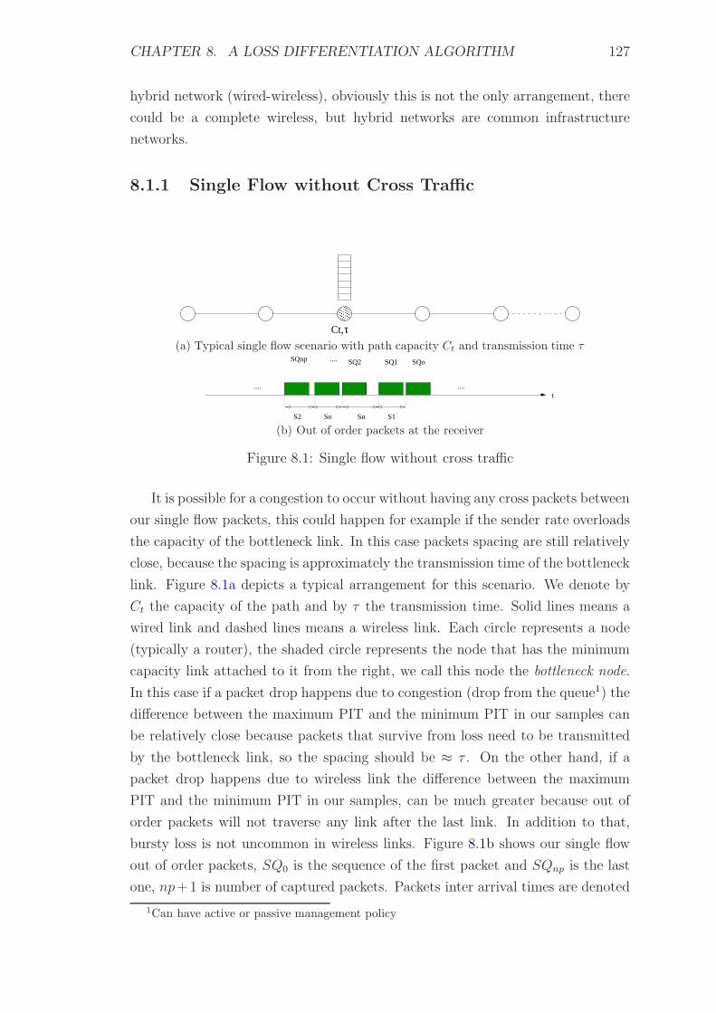
CHAPTER 8. A LOSS DIFFERENTIATION ALGORITHM 127
hybrid network (wired-wireless), obviously this is not the only arrangement, there
could be a complete wireless, but hybrid networks are common infrastructure
networks.
8.1.1 Single Flow without Cross Traffic
���������
���������
Ct, τ(a) Typical single flow scenario with path capacity Ct and transmission time τ
t
SnSoS2 S1
SQoSQ1SQ2....SQnp
.... ....
(b) Out of order packets at the receiver
Figure 8.1: Single flow without cross traffic
It is possible for a congestion to occur without having any cross packets between
our single flow packets, this could happen for example if the sender rate overloads
the capacity of the bottleneck link. In this case packets spacing are still relatively
close, because the spacing is approximately the transmission time of the bottleneck
link. Figure 8.1a depicts a typical arrangement for this scenario. We denote by
Ct the capacity of the path and by τ the transmission time. Solid lines means a
wired link and dashed lines means a wireless link. Each circle represents a node
(typically a router), the shaded circle represents the node that has the minimum
capacity link attached to it from the right, we call this node the bottleneck node.
In this case if a packet drop happens due to congestion (drop from the queue1) the
difference between the maximum PIT and the minimum PIT in our samples can
be relatively close because packets that survive from loss need to be transmitted
by the bottleneck link, so the spacing should be ≈ τ . On the other hand, if a
packet drop happens due to wireless link the difference between the maximum
PIT and the minimum PIT in our samples, can be much greater because out of
order packets will not traverse any link after the last link. In addition to that,
bursty loss is not uncommon in wireless links. Figure 8.1b shows our single flow
out of order packets, SQ0 is the sequence of the first packet and SQnp is the last
one, np+1 is number of captured packets. Packets inter arrival times are denoted
1Can have active or passive management policy

CHAPTER 8. A LOSS DIFFERENTIATION ALGORITHM 128
by S, where S0 ≤ S1 ≤ S2 . . . ≤ Sn and the number of samples is n+1. In this case
S ≈ τ , if we plot the distribution of the PITs we get a single major spike at the
transmission time of the bottleneck capacity, τ . In our discussion a “major spike”
is synonym to a “pattern”. So in this situation we have small difference between
the maximum and minimum PITs and a pattern. The discriminator decision based
on the difference between the maximum and minimum PITs appears to be valid
in this case.
8.1.2 Single Flow with Cross Traffic
It is possible to have cross traffic joining our single flow packets during their
travel from source to destination across the multi hop path and exit the path
at some point later, cross traffic interference during congestion (queue build-up)
adds randomness to our single flow PIT, this is due to queue build-up and queue
empty processes, because each cross traffic packet that interferes with the single
flow packets represent a time gap in future time (when the cross traffic packet
exits the path) these time gaps are subject to variations along the path, starting
from the random arrival of cross traffic then bottleneck node processing time, any
other future queue build-up, or other cross traffic, etc. In addition to that cross
traffic packets can have different sizes (e.g. ACK packets which have smaller size).
If packet loss happens in this situation (likely due to congestion), an ambiguity
appears: is the difference between the maximum and minimum PITs due to cross
traffic interference or is it the large difference that appears in a non-congestive
loss (when there is at least one large gap in PITs and the rest are small i.e.
back-to-back)?
To help resolving this, we use another signal which we believe it is coupled with
the existence of cross traffic, we expect the single flow PITs in our captured sample
to have significant randomness due to cross traffic interference during congestion.
In contrast, if there is no congestion (queue build-up) and a packet drop happens
(likely due to wireless link transmission error), the single flow PITs in our captured
sample are expected to have less randomness, since the packets are dropped at the
last link, the time gaps have less chance to change and the PITs are approximately
multiples of the bottleneck link transmission time (depending on how many packet
drops happened at the last link). Therefore, this randomness in PITs can help our
discriminator to make the discussion about the type of packet loss in this case.
Two points to note here: Firstly, lower layer wireless protocols adds random-
ness to both situations. Secondly, an intuitive question that stems from the above
discussion is: What if a packet drop due to wireless link transmission error happens
during congestion? Since the overall pattern is random in a congestion situation

CHAPTER 8. A LOSS DIFFERENTIATION ALGORITHM 129
the packet drop will be assumed to be due to congestion. In fact it is better to
be conservative in our assumptions, it has been shown [15] that it is much more
costly to mistakenly identify a congestive loss as a non-congestive one than the
other way round.
Another point to mention is that it is possible to have a cross traffic interference
without having a congestion, this means that either there is no queue build-up or
the queue build-up and empty between two single flow packets (before the second
packet arrive at the node), both situations have limited effect on the pattern.
Any packet drop in this case will be recognised as wireless link transmission error
based on case B. Note that the network is not congested here, this can be viewed
as temporary or transient congestion that disappears after a short time.
8.2 PITs Distributions
In this section we examine different PITs distributions in existence and absence
of cross traffic. Where spikes are considered patterns, the areas between these
spikes, in fact; constitute the randomness2 that we were talking about. Hence, the
wider the spectrum, the more likely to have randomness in PITs. Our aim in this
section is to show that cross traffic interference can have this wide spectrum.
8.2.1 Single Flow without Cross Traffic
Referring to figure 8.1, in normal operation; our single flow packets arrive back-to-
back at the receiver separated by the bottleneck transmission time, maintaining
the assumption that the sender performs bulk data transfer, the PIT distribution
is expected to have single spike at the bottleneck transmission time, in this case
τ .
8.2.2 Single Flow with Cross Traffic
There are many scenarios where this could happen, we break these into six sce-
narios (other scenarios can be combinations of these six scenarios). In figure 8.2
all the conventions in figure 8.1a apply. It is possible to have a queue build-up at
Ct, but we are not showing this queue to avoid confusion with the queue build-
up due to cross traffic. The bottleneck transmission time is denoted by Tc, the
transmission time of the link attached to right to the node which has significant
queueing due to cross traffic is denoted by τ , in case there are more than one, they
2In reality, there are minor i.e. very small spikes between the major spikes, we refer to theseas “areas” without drawing them, so the term “spike” can retain the meaning of a pattern. Plotsfrom real experiments are available in literature [59]

CHAPTER 8. A LOSS DIFFERENTIATION ALGORITHM 130
��������
��������
cross traffic
τ
Ct
(a) Scenario 1
������������
������������
cross traffic
Ct,τ
(b) Scenario 2
������������
������������
cross traffic
τCt
(c) Scenario 3
���������
���������
cross traffic
Ct τ1 τ2
cross traffic
(d) Scenario 4
��������
��������
cros
s tra
ffic
τ2
cros
s tra
ffic
Ct,τ1
(e) Scenario 5
������������
������������
cros
s tra
ffic
cros
s tra
ffic
Ct,τ1 τ2
(f) Scenario 6
Figure 8.2: Single flow with cross traffic
are denoted by τ1, τ2, . . .. The flow of packets is from the left to the right, with
our single flow packets arriving with an initial time spacing denoted by Ti at the
first node from the left and determined by the minimum transmission time in the
path traversed so far (not shown in the figure) and packet size, however if the first
node from the left is the sender, then Ti is determined only by sender rate and
packet size. In scenarios 1-6, Tc ≥ Ti, Tc ≥ τ
In the analysis of these scenarios we are concerned in a three major points:
• The location of the bottleneck node;
• The location of the queue due to cross traffic;
• The packet drop event (discussed in the next section).
We leave the last point to the next section. Let us start by looking at scenario 1,
our single flow packets get re-spaced from Ti to Tc at the bottleneck node (first
from left in figure 8.2a), then they are queued at the third node where cross traffic
starts joining our packets in their journey to the destination. Due to cross traffic
interference and queue build-up, PITs get expanded or squeezed3 by multiples
of τ depending on the degree of congestion. Some practical cases that illustrate
this behaviour are shown in [59]. As a result, the distribution of PIT is expected
to have a major spike at Tc (because queueing is transient and most packets will
arrive spaced approximately by the bottleneck transmission time Tc in the absence
of the queue at node three) and minor spikes at the multiples of τ . Please see
figure 8.3a, scenario 1. It is not necessary for the spikes to be symmetrical, this
could depend on the severity of cross traffic interference but several symmetrical
cases were reported in practical measurements made in [59].
Scenario 2 can be analysed similarly, but now cross traffic joins our single flow
packets at the the bottleneck node, thus Tc = τ , PITs get expanded but cannot get
3Note that squeezing could happen if single flow packets queue behind cross traffic packetsand is possible because τ is less than Tc

CHAPTER 8. A LOSS DIFFERENTIATION ALGORITHM 131
squeezed (less than Tc), the distribution of PIT is expected to have a major spike
at Tc and minor spikes at the multiples of it only from the right. See figure 8.3a,
scenario 2.
In scenario 3, the cross traffic joins our single flow packets before the bottleneck
node, so the queueing at the second node disturbs the initial PIT, Ti by expanding
and squeezing at multiples of τ . However, after passing the bottleneck link things
change depending on the amount of of expansion in Ti. If Tc > Ti + nτ , where n
is the number of cross traffic in between, the bottleneck link re-spaces the packets
to Tc. If Tc < Ti + nτ , then packets can escape from the bottleneck link without
being re-spaced. The distribution of PIT is expected to have only one major spike
at Tc when Tc > Ti + nτ and a major spike at Tc followed by one minor spike on
the right at a random time determined by n in Ti +nτ , we denote this by X. After
that, minor spikes at multiples of τ could appear on the right. See figure 8.3a,
scenario 3.
Scenario 4 can be seen as a combination of scenario 1 and scenario 3, in this
case we have two queues due to cross traffic, one at node one and the other at
node four, each followed by two links with transmission times of τ1, τ2 respectively,
and the bottleneck is in between. We analyse the case where τ1 > τ2. Before the
bottleneck node, the initial packets spacing Ti gets expanded and squeezed by τ1
at node one, again squeezing is possible because τ1 is less than Ti. If no packets
escape from the bottleneck link re-spacing (as in scenario 3) then all packets leave
the bottleneck link re-spaced by Tc. After the bottleneck node our single flow
packets still have one queue barrier at node four where again their spacing gets
expanded and squeezed by τ2, squeezing is possible because τ2 is less than Tc.
However if some packets escaped with a spacing of Tc > Ti + nτ1 each can get
further expanded or squeezed by τ2, squeezing is possible because τ2 is less than
their spacing. See figure 8.3b, scenario 4. figure 8.3c scenario 4, depicts the case
when τ1 < τ2.
Scenario 5 can be seen as a combination of scenario 1 and scenario 2, in this
case we have two queues due to cross traffic, one at the bottleneck node (node
two) and the other at node four, each followed by two links with transmission
times of τ1 = Tc, τ2 respectively. We analyse the case where τ1 > τ2. Before the
second queue, the single flow packets are spaced by τ1 or expanded by multiples
of it (similar to scenario 2), each of these spacings can get squeezed or expanded
by multiples of τ2 (note that they might remain unchanged in the absence of the
second queue, but here we are considering a queue build-up). See figure 8.3b,
scenario 5. figure 8.3c scenario 5, depicts the case when τ1 < τ2.
Finally, scenario 6 can be seen as a combination of scenario 2 and scenario 3,
since Tc = τ2 > τ1, the second queue is expected to dominate the packet spacing

CHAPTER 8. A LOSS DIFFERENTIATION ALGORITHM 132
ττTcTc
= Tc
Tiτ
Tc Tcχ τ
Tc < Ti + nτ
Ti + nτ
Tc > Ti + nτ
[2][1]
Before Ct :
After Ct :
[3]
(a) Scenarios 1-3.
Ti
Tc
τ1
τ1
τ2
Ti + nτ1
Tc < Ti + nτ1
τ2
Tc > Ti + nτ1
Tcτ2
χ
τ2
Before Ct :
After Ct :
τ1 τ1
τ2 τ2 τ2
[5]
[4]
(b) Scenarios 4-6, τ1 > τ2.
Ti
Tc
τ1Ti + nτ1
Tc < Ti + nτ1
τ2
Tc > Ti + nτ1
Tc
χ
Before Ct :
After Ct :
Tc = τ2
τ1 τ2
τ2
τ1 τ1
τ2 τ2 τ2
[6][5]
[4]
(c) Scenarios 4-6, τ1 < τ2.
Figure 8.3: Hypothetical PIT distributions for scenarios 1-6.
in this scenario, most packets are expected to arrive spaced by the bottleneck
transmission time Tc along with other expanded (but not squeezed) in time at
multiples of τ2. figure 8.3c scenario 6, depicts the PITs distribution.
As mentioned before, there are other scenarios, for example having two or more
queues (due to cross traffic) before the bottleneck, or after it. This adds more time
spacing variations and the analysis of such cases will not add to the discussion;
since we have already seen similar time spacing variations in the six scenarios.
Most of these scenarios have a wide spectrum of PITs and the areas between their
distribution spikes are potential values for PIT, i.e. PIT can take values between
these spikes in reality, see for example [59]. We believe that this supports our
assumption about randomness in PITs during cross traffic interference.
8.3 Analysis with Packet Drop
In this section we analyse the case of single flow without cross traffic and scenario 2
of the other case, we also explain a new technique which we use for extracting the

CHAPTER 8. A LOSS DIFFERENTIATION ALGORITHM 133
noise from the samples in order to quantify it.
8.3.1 Single Flow without Cross Traffic
The cases mentioned before are ideal cases, they are mentioned for pedagogical
purposes to illustrate the concept. In reality PITs are not separated exactly by
fixed time spaces, this is due to variations in the delay along the path: propaga-
tion delay, queueing delay, packet re-spacing, node processing times, in addition
to packet re-spacing that can take place along the path, lower layer protocols
behaviour (e.g. frame retransmission, not significant in wired links compared to
wireless links), in addition to cross traffic interference during congestion, where a
packet could arrive while the another is being served4. To take this into account,
we assign a noise factor ±δ to each sample. We looked at single flow out of order
packets in figure 8.1b, we refer the same figure in our discussion. There are np+1
packets and their sequence numbers are denoted by: SQ0 . . . SQnp and captured
upon a packet loss trigger. Samples are denoted by: S0 ≤ S1 ≤ S2 . . . ≤ Sn. Each
sample is represented as: xT ± δ, where:
T : Packet transmission time of the minimum capacity link in the path (all packets
arrive back to back spaced by this time in normal operation);
x: Number of multiples of T , ∈ Z+;
x0 ≤ x1 ≤ x2 . . . ≤ xn, xi ≤ xi+l, 0 < x0 ≤ xi ≤ xn, 0 ≤ i ≤ n;
Smin = x0T ± δ0 and Smax = xnT ± δn;
δ: Noise factor, δ ≪ T ;
np: Maximum number of packets. ∈ Z+;
nℓi: Number of lost packets in each sample (between two out of order packets),∈Z+, 0 ≤ i ≤ n;
n: Maximum number of PITs (samples) to be analysed. n ∈ Z+;
n = np− 1;
xi = nℓi + 1.
Because out of order packets arrive spaced by ≈ T in case of congestion, and ≈ xT ,
x > 1 in case of wireless loss, we rely on the span 1− Smin/Smax (we explain this
formula later on in this chapter) to discriminate the type of loss in this case. A
large span indicates a wireless loss and a small one indicates congestive loss.
8.3.2 Single Flow with Cross Traffic
This section includes the analysis of scenario 2 in the presence of packet drop.
Scenario 2 was chosen for its simplicity, since most of the events happen at the
4This affects the time spacing between packets [59], which we will rely upon in discriminatingthe type of packet loss.

CHAPTER 8. A LOSS DIFFERENTIATION ALGORITHM 134
........
SQoSQ2 SQ1....SQnp
SnS2SoS1
t
t
........
TT T T
Figure 8.4: scenario 2, bottom: cross traffic and packet drop, top: after crosstraffic leaves the path.
same location (the bottleneck node).
Each sample is represented as xT ± δ, where T = Tc = τ . Figure 8.4 depicts
a hypothetical PIT pattern for this scenario. Single flow packets have the green
colour, and cross traffic have the yellow colour. Lost packets from both have a red
contour. The samples are:
S0 = x0T ± δ0
S1 = x1T ± δ1
S2 = x2T ± δ2
...
Sn = xnT ± δn
(8.1)
If the packet drop happens due to congestion, the noise factor is expected to have
large values compared to the case where it happens due to wireless link errors. In
subsection 8.3.1 we used a quantified measure (the span) we shall find a way to
quantify the noise factor in order to make a decision. Our first goal is to extract
the noise factor (δs) from our samples, then as a second goal, to find a way to
quantify the collected δs.
In order to extract the noise factor from the samples, we propose a recursive
technique and call it a “Difference Canceller”, the basic idea is to subtract all
possible different combinations of the samples from each other, because xT takes
finite values, after repeating the process for a certain number of iterations, the term
xT diminishes at the same time the technique dumps residual terms (those less
than T ) each iteration. The block diagram in figure 8.5 depicts the operation of the
recursive technique. The process continues until sufficient T terms are cancelled;
leaving the residual noise factor terms. It can be shown that the maximum sample

CHAPTER 8. A LOSS DIFFERENTIATION ALGORITHM 135
S1
S2
S3
Si
SnSn−1
Sj
S2
S1
S0 |S1−S0|
|S2−S0|, |S2−S1|
|S3−S0|, |S3−S1|, |S3−S2|
|Si−S0|, |Si−S1|, ..., |Sj−Si|
Figure 8.5: Difference Canceller
of the next iteration is always less than the maximum sample of the previous
iteration, which means that the technique converges towards T . Now, we apply the
technique to scenario 2, let k be the number of iterations, recall that T = Tc = τ ,
we define di,j to be the absolute difference between two samples, by taking all
different possible combinations of samples we obtain a set ∆k for each iteration,
where:
di,j = |Si − Sj| , when k = 1, 0 ≤ j ≤ n− 1. (8.2)
∆k = {di,j}i>j , when k = 1, j < i ≤ n. (8.3)
We need the number of samples in each iteration to calculate all possible dif-
ferent combinations, for example; for the first iteration:
(n + 1
2
)
=(n + 1)!
2!(n− 1)!=
(n + 1)n
2
All output samples in ∆k are considered inputs for the next iteration. The number
of the new samples is n′ + 1, where n′ + 1 = (n + 1)n/2, therefore there are
S ′0, S′1, S
′1 . . . S ′n′
The samples for the next iteration are:
S ′0 = |(x1 − x0)T ± δ1 ∓ δ0|S ′1 = |(x2 − x0)T ± δ2 ∓ δ0|
...

CHAPTER 8. A LOSS DIFFERENTIATION ALGORITHM 136
S ′n−1 = |(xn − x0)T ± δn ∓ δ0|S ′n = |(x2 − x1)T ± δ2 ∓ δ1|
...
S ′n′−1 = |(xn − xn−2)T ± δn ∓ δn−2|S ′n′ = |(xn − xn−1)T ± δn ∓ δn−1|
(8.4)
Below is the first and second iterations, the number to the right is the number of
samples of the jth set. One point to note here is that some noise factors can get
cancelled in a sample due to the subtraction process but this doesn’t mean that
they are lost, because they appear in other samples, thus the information of this
noise factor is reserved by the additive term in other samples, this can be seen for
example in the second iteration when j′ = 0, δ0 is cancelled in some terms, but it
sill appear in other samples, like the last one. In other words there is a redundancy
and the noise factor information is conveyed throughout the iterations, unlike the
the xT terms which diminish throughout the iterations:
k=1
j = 0
d1,0 = |(x1 − x0)T ± δ1 ∓ δ0|d2,0 = |(x2 − x0)T ± δ2 ∓ δ0|d3,0 = |(x3 − x0)T ± δ3 ∓ δ0|...
di,0
...
dn,0 = |(xn − x0)T ± δn ∓ δ0|
n
j = 1
d2,1 = |(x2 − x1)T ± δ2 ∓ δ1|d3,1 = |(x3 − x1)T ± δ3 ∓ δ1|d4,1 = |(x4 − x1)T ± δ4 ∓ δ1|...
di,1
...
dn,1 = |(xn − x1)T ± δn ∓ δ1|
n− 1

CHAPTER 8. A LOSS DIFFERENTIATION ALGORITHM 137
...
di,j = |(xi − xj)T ± δi ∓ δj |...
n− j
j = n− 2
{
dn−1,n−2 = |(xn−1 − xn−2)T ± δn−1 ∓ δn−2|dn,n−2 = |(xn − xn−2)T ± δn ∓ δn−2|
2
j = n− 1{
dn,n−1 = |(xn − xn−1)T ± δn ∓ δn−1| 1
k=2
j′ = 0
d1,0 = |(x2 − x1)T ± δ2 ∓ δ0 ∓ δ1 ± δ0|d2,0 = |(x3 − x1)T ± δ3 ∓ δ0 ∓ δ1 ± δ0|d3,0 = |(x4 − x1)T ± δ4 ∓ δ0 ∓ δ1 ± δ0|...
di′,0
...
dn′,0 = |(xn − xn−1 − x1 + x0)T ± δn ∓ δn−1 ∓ δ1 ± δ0|
n′
j′ = 1
d2,1 = |(x3 − x2)T ± δ3 ∓ δ0 ∓ δ2 ± δ0|d3,1 = |(x4 − x2)T ± δ4 ∓ δ0 ∓ δ2 ± δ0|d4,1 = |(x5 − x2)T ± δ5 ∓ δ0 ∓ δ2 ± δ0|...
di′,1
...
dn′,1 = |(xn − xn−1 − x2 + x0)T ± δn ∓ δn−1 ∓ δ2 ± δ0|
n′ − 1
j′ = n−1
dn,n−1 = |Sn − Sn−1| = |(xn − x0 − x2 + x1)T ± δn ∓ δ0 ∓ δ2 ± δ1|...
dn′,n−1 = |Sn′ − Sn−1| = |(xn − x0 − xn + xn−1)T ± δn ∓ δ0 ∓ δn ± δn−1|= |(xn−1 − x0)T ± δn ∓ δ0 ∓ δn ± δn−1|
n′ − n + 1
...
di′,j′ = |(xi′ − xj′)T ± δi′ ∓ δj′|...
n′ − j′

CHAPTER 8. A LOSS DIFFERENTIATION ALGORITHM 138
j′ = n′−2
dn′−1,n′−2 = |(xn − xn−2 − xn−1 + xn−2)T ± δn ∓ δn−2 ∓ δn−1 ± δn−2|= |(xn − xn−1)T ± δn ∓ δn−2 ∓ δn−1 ± δn−2|
dn′,n′−2 = |(xn − xn−1 − xn−1 + xn−2)T ± δn ∓ δn−1 ∓ δn−1 ± δn−2|= |(xn − 2xn−1 + xn−2)T ± δn ∓ δn−1 ∓ δn−1 ± δn−2|
2
j′ = n′−1
{
dn′,n′−1 = |(xn − xn−1 − xn + xn−2)T ± δn ∓ δn−1 ∓ δn ± δn−2|= |(xn−1 − xn−2)T ± δn ∓ δn−1 ∓ δn ± δn−2|
1
It can be shown using simple algebra that the finite term xT in our samples
cancel as the number of iterations increase. We refer to this as “convergence of
the algorithm”. We state the proof of convergence as follows:
Proof. Let Smax be the initial maximum sample and S ′max, S′′max, . . . be the maxi-
mum samples of the first, second, . . . iterations respectively. Similarly, Smin be the
initial minimum sample and S ′min, S ′′min, . . . be the minimum samples of the first,
second, . . . iterations respectively. We already know that:
Smax = xnT ± δn
Smin = x0T ± δ0
(8.5)
And using equation 8.2:
S ′max = |Smax − Smin|S ′′max = |S ′max − S ′min|
...
(8.6)
Given that T ≫ δ and 0 < x0 < xn, then:
x0 > 0
−x0 < 0
xn − x0 < xn
|(xn − x0)T | < |xnT |, T > 0
|(xn − x0)T ± δn ∓ δ0| < |xnT ± δn|, T ≫ δ

CHAPTER 8. A LOSS DIFFERENTIATION ALGORITHM 139
∴ S ′max < Smax
(8.7)
Following a similar semantic for the next iteration, here S ′min is not precisely
known, only its range is known:
S ′max = |(xn − x0)T ± δn ∓ δ0|S ′min = |(yp − yq)T ± δp ∓ δq|
(8.8)
Where, 0 < x0 ≤ yq ≤ yp ≤ xn. Now using equation 8.2 and equation 8.6 we get:
|yp − yq| > 0
−|yp − yq| < 0
|xn − x0| − |yp − yq| < |xn − x0|(|xn − x0| − |yp − yq|)T < (|xn − x0|)T, T > 0
|(|xn − x0| − |yp − yq|)T ±δn ∓ δ0 ∓ δyp ± δyq︸ ︷︷ ︸
≪ T
| < |(|xn − x0|)T ± δn ∓ δ0|, T ≫ δ
∴ S ′′max < S ′max
(8.9)
And:
. . . < S(k+3)max < S(k+2)
max < S(k+1)max < S(k)
max < Smax (8.10)
Note, that for this proof to hold, the condition: T ≫∑
δ in each iteration is
necessary.

CHAPTER 8. A LOSS DIFFERENTIATION ALGORITHM 140
Example (scenario 2):
S3S2SoS1
t
SQ4 SQ1 SQoSQ2SQ3
Figure 8.6: Scenario 2 example, PIT of five packets.
In this example, {SQ1, SQ2} 6= SQ0 + 1, and we captured five packets, thus
np + 1 = 5, np = 4 and n = np − 1 = 4− 1 = 3. The samples to be analysed in
the first iteration (k = 1) are:
S0 = T ± δ0
S1 = 2T ± δ1
S2 = 3T ± δ2
S3 = 4T ± δ3
Calculating the differences using equation- 8.2 and equation- 8.3:
di,j = |Si − Sj| , when k = 1, 0 ≤ j ≤ 2.
∆1 = {di,j}i>j , when k = 1, j < i ≤ 3.
d1,0 = |S1 − S0| = |2T ± δ1 − T ∓ δ0| = |T ± δ1 ∓ δ0|d2,0 = |S2 − S0| = |3T ± δ2 − T ∓ δ0| = |2T ± δ2 ∓ δ0|d3,0 = |S3 − S0| = |4T ± δ3 − T ∓ δ0| = |3T ± δ3 ∓ δ0|d2,1 = |S2 − S1| = |3T ± δ2 − 2T ∓ δ1| = |T ± δ2 ∓ δ1|d3,1 = |S3 − S1| = |4T ± δ3 − 2T ∓ δ1| = |2T ± δ3 ∓ δ1|d3,2 = |S3 − S2| = |4T ± δ3 − 3T ∓ δ2| = |T ± δ3 ∓ δ2|
Now, the number of input samples for the next iteration (k = 2) is: n′ + 1 =
n(n + 1)/2 = 3× 4/2 = 6, n′ = 5.
S ′0 = T ± δ1 ∓ δ0
S ′1 = T ± δ2 ∓ δ1
S ′2 = T ± δ3 ∓ δ2
S ′3 = 2T ± δ2 ∓ δ0
S ′4 = 2T ± δ3 ∓ δ1
S ′5 = 3T ± δ3 ∓ δ0
Calculating the differences for the new iteration using equation 8.2 and equa-
tion 8.3:
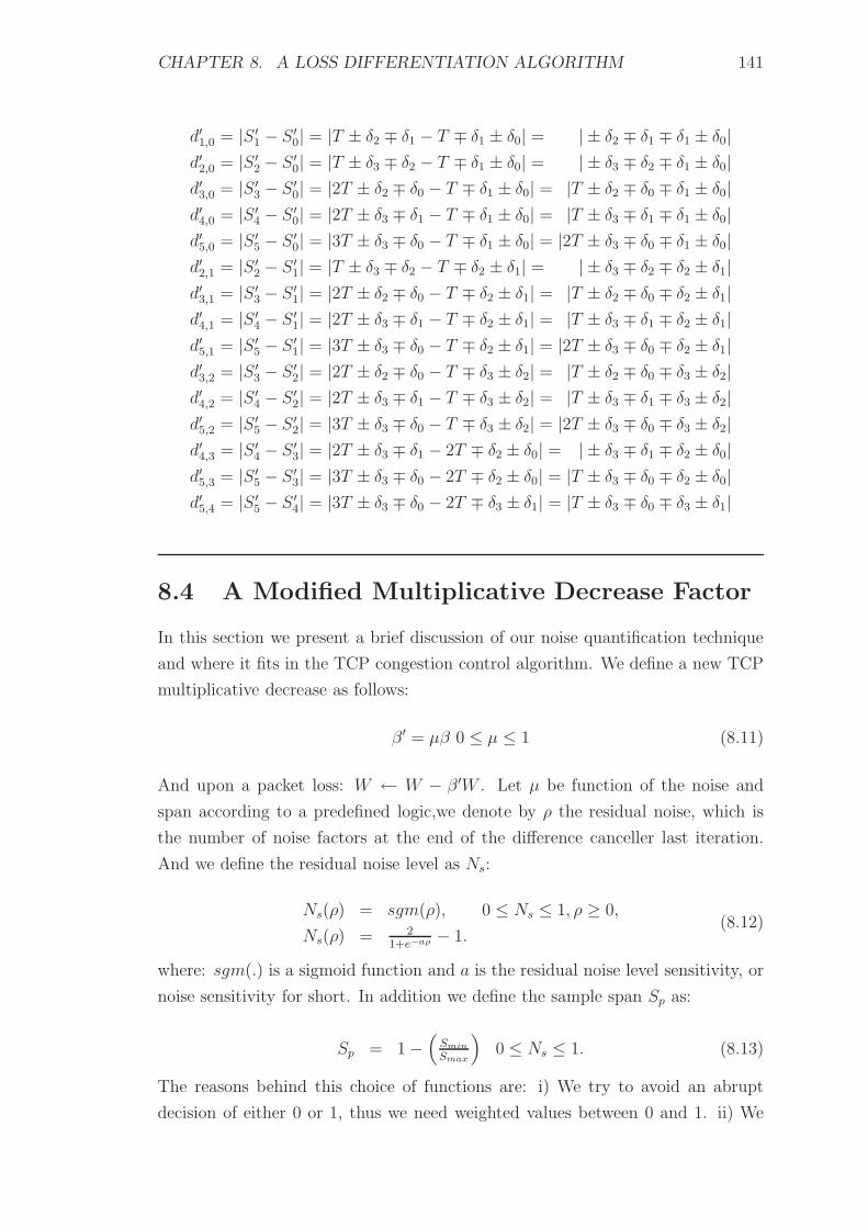
CHAPTER 8. A LOSS DIFFERENTIATION ALGORITHM 141
d′1,0 = |S ′1 − S ′0| = |T ± δ2 ∓ δ1 − T ∓ δ1 ± δ0| = | ± δ2 ∓ δ1 ∓ δ1 ± δ0|d′2,0 = |S ′2 − S ′0| = |T ± δ3 ∓ δ2 − T ∓ δ1 ± δ0| = | ± δ3 ∓ δ2 ∓ δ1 ± δ0|d′3,0 = |S ′3 − S ′0| = |2T ± δ2 ∓ δ0 − T ∓ δ1 ± δ0| = |T ± δ2 ∓ δ0 ∓ δ1 ± δ0|d′4,0 = |S ′4 − S ′0| = |2T ± δ3 ∓ δ1 − T ∓ δ1 ± δ0| = |T ± δ3 ∓ δ1 ∓ δ1 ± δ0|d′5,0 = |S ′5 − S ′0| = |3T ± δ3 ∓ δ0 − T ∓ δ1 ± δ0| = |2T ± δ3 ∓ δ0 ∓ δ1 ± δ0|d′2,1 = |S ′2 − S ′1| = |T ± δ3 ∓ δ2 − T ∓ δ2 ± δ1| = | ± δ3 ∓ δ2 ∓ δ2 ± δ1|d′3,1 = |S ′3 − S ′1| = |2T ± δ2 ∓ δ0 − T ∓ δ2 ± δ1| = |T ± δ2 ∓ δ0 ∓ δ2 ± δ1|d′4,1 = |S ′4 − S ′1| = |2T ± δ3 ∓ δ1 − T ∓ δ2 ± δ1| = |T ± δ3 ∓ δ1 ∓ δ2 ± δ1|d′5,1 = |S ′5 − S ′1| = |3T ± δ3 ∓ δ0 − T ∓ δ2 ± δ1| = |2T ± δ3 ∓ δ0 ∓ δ2 ± δ1|d′3,2 = |S ′3 − S ′2| = |2T ± δ2 ∓ δ0 − T ∓ δ3 ± δ2| = |T ± δ2 ∓ δ0 ∓ δ3 ± δ2|d′4,2 = |S ′4 − S ′2| = |2T ± δ3 ∓ δ1 − T ∓ δ3 ± δ2| = |T ± δ3 ∓ δ1 ∓ δ3 ± δ2|d′5,2 = |S ′5 − S ′2| = |3T ± δ3 ∓ δ0 − T ∓ δ3 ± δ2| = |2T ± δ3 ∓ δ0 ∓ δ3 ± δ2|d′4,3 = |S ′4 − S ′3| = |2T ± δ3 ∓ δ1 − 2T ∓ δ2 ± δ0| = | ± δ3 ∓ δ1 ∓ δ2 ± δ0|d′5,3 = |S ′5 − S ′3| = |3T ± δ3 ∓ δ0 − 2T ∓ δ2 ± δ0| = |T ± δ3 ∓ δ0 ∓ δ2 ± δ0|d′5,4 = |S ′5 − S ′4| = |3T ± δ3 ∓ δ0 − 2T ∓ δ3 ± δ1| = |T ± δ3 ∓ δ0 ∓ δ3 ± δ1|
8.4 A Modified Multiplicative Decrease Factor
In this section we present a brief discussion of our noise quantification technique
and where it fits in the TCP congestion control algorithm. We define a new TCP
multiplicative decrease as follows:
β ′ = µβ 0 ≤ µ ≤ 1 (8.11)
And upon a packet loss: W ← W − β ′W . Let µ be function of the noise and
span according to a predefined logic,we denote by ρ the residual noise, which is
the number of noise factors at the end of the difference canceller last iteration.
And we define the residual noise level as Ns:
Ns(ρ) = sgm(ρ), 0 ≤ Ns ≤ 1, ρ ≥ 0,
Ns(ρ) = 21+e−aρ − 1.
(8.12)
where: sgm(.) is a sigmoid function and a is the residual noise level sensitivity, or
noise sensitivity for short. In addition we define the sample span Sp as:
Sp = 1−(
Smin
Smax
)
0 ≤ Ns ≤ 1. (8.13)
The reasons behind this choice of functions are: i) We try to avoid an abrupt
decision of either 0 or 1, thus we need weighted values between 0 and 1. ii) We

CHAPTER 8. A LOSS DIFFERENTIATION ALGORITHM 142
need a a tunable function for the noise factor since the amount of noise that is
needed to make a decision is still vague and a tunable function is desirable for
experimental purposes, an attractive choice of functions is the sigmoid, where we
can change the value between 0 and 1 and tune it using a. iii) On the other hand
the amount of span needed to make a decision depends on the ratio of minimum
to maximum values of a sample thus it is logical to use a simple linear function of
the ratio, also note that taking the ratio (not the difference) makes the function’s
output unit less (i.e. not in seconds).
Let µ(Ns, Sp). We now find the relation between µ and Ns, Sp using the logic
in table 8.1. This logic is in fact a translation of our assumptions.
Table 8.1: Relation between Noise level [Ns], Samples Span [Sp] and Output [µ]
Sp Ns Output [µ] Type of Loss
↓ ↓ ↑ congestive loss↓ ↑ ↑ congestive loss↑ ↓ ↓ wireless loss↑ ↑ ↑ congestive loss
µ = ¬Sp + Ns,
= 1− Sp + Ns,(8.14)
Substituting for Ns Sp using equations 8.12, 8.13: µ(ρ, Smin, Smax) =
=Smin(1 + e−aρ)− Smax(1 + e−aρ) + 2
Smax(1 + e−aρ)(8.15)
8.5 Simulation Experiments & Results
In this section we present some of our simulation results. Nodes were arranged
as in scenario 2 (please see figure 8.2b), with link capacities from left to right:
4 Mbps, 5 Mbps, 3 Mbps, 4 Mbps and 5 Mbps. Each having 10ms propagation
delay. We used single TCP flow, where the source performs a bulk transfer for
one minute of simulation time. A group of: 10, 50 and 100 UDP cross traffic
sources enter the network route randomly and interfere with the TCP flow during
the one minute. Each cross traffic source sends data at rate of 0.3 Mbps and each
cross traffic link has a capacity of 1 Mbps with randomly assigned propagation
delays. We used an error model at the last link to simulate the behaviour of a
lossy wireless link. At the bottleneck link we used ordinary Drop-Tail queue with
buffer size of 5 packets. We did not take the effect of variable packets size of cross
traffic into account in our experiments and used a fixed packet size of 1000 bytes

CHAPTER 8. A LOSS DIFFERENTIATION ALGORITHM 143
for both TCP flow and UDP cross traffic.
Table 8.2: Loss probabilities used in Group 2 and Group 3 experiments
Experiment Congestive loss (%) Wireless loss (%)
1 0.465371 0.6345372 0.826583 0.9427253 0.911279 1.005854 0.79264 0.9427255 0.80507 0.9427256 0.379205 0.5354387 1.05028 1.325058 0.541859 0.7436159 0.827519 0.94272510 1.04483 1.32505
The aim is to validate our assumptions and the logical formula that we have
used, in order to do that, we run three groups of simulation experiments, 10
experiments for each group, Group 1: no cross traffic, no wireless loss, Group 2:
cross traffic without wireless loss, Group 3: wireless loss without cross traffic. By
examining the resultant values of the new multiplicative decrease factor β ′, noise
and span, we can achieve our aim as follows: the TCP flow in Group 2 suffers only
from congestive loss and thus its β ′ values are expected to have large values. In
contrast, the TCP flow in Group 3 suffers mainly from wireless loss and thus its β ′
values are expected to have small values. The arguments for noise and span and
their assumptions are mutatis mutandis to that of the new multiplicative decrease
factor β ′.
In the absence of any cross traffic and wireless loss (Group 1) we noticed that
the network suffered from a packet loss probability = 0.00950841% (caused by
standard TCP CC operation). Table 8.2 shows the packet loss probabilities used
in the 10 experiments of Group 2 (second column) and the 10 experiments of
Group 3 (third column). These probabilities were obtained as follows: we first
run Group 2 experiments, we select a number of cross traffic sources, run the first
experiment, calculate the packet loss probability, then run the second experiment
and do the same, and so on until the tenth experiment. Second, we run Group 3
experiments, but in this group we need to set the random loss model, we used
the values obtained from Group 2 experiments in this model. We set the loss
probability to the value obtained from the first experiment from Group 2 and
run the first experiment then calculate the loss probability, then we set the loss
probability to the value obtained from the second experiment from Group 2 and
run the second experiment then calculate the loss probability and so on until the
tenth experiment.
Steps in bullet points are:

CHAPTER 8. A LOSS DIFFERENTIATION ALGORITHM 144
• Nodes were arranged as in scenario 2
• Link capacities from left to right: 4 Mbps, 5 Mbps, 3 Mbps, 4 Mbps and 5
Mbps
• Each having 10ms propagation delay
• Single TCP flow, one minute bulk transfer
• A group of: 10, 50 and 100 UDP randomly interfere with the TCP flow
• Cross traffic rates are 0.3 Mbps and each link has a capacity of 1 Mbps with
randomly assigned propagation delays
• We used an error model at the last link to simulate the behaviour of a lossy
wireless link
• At the bottleneck link we used drop tail queue discipline with buffer size of
5 packets
• Fixed packet size of 1000 bytes for both TCP flow and UDP cross traffic
• We did not take the effect of variable packets size and lower layers into
account in our experiments
• We run three groups of simulation experiments, 10 experiments for each
group
• Group 1: no cross traffic, no wireless loss
• Group 2: cross traffic without wireless loss
• Group 3: wireless loss without cross traffic
After that we run a non-implemented version of the modified TCP-Reno which is
part of our TCP post-simulation analysis tool that we developed to test our work.
The tool does packet drop statistics, TCP parameters calculations, runs the new
technique and generates 15 graphs representing the results. We set the Difference
Canceller to work for one iteration i.e. k = 1 and the noise sensitivity a = 1. Steps
in bullet points:
• Non-implemented version of the modified TCP-Reno as part of our TCP
post-simulation analysis tool
• We set the Difference Canceller to work for one iteration i.e. k = 1 and the
noise sensitivity a = 1

CHAPTER 8. A LOSS DIFFERENTIATION ALGORITHM 145
0
0.1
0.2
0.3
0.4
0.5
1 10 100
β’
Loss detected by duplicate ACKs
Total Variable M.D. -- congestive loss caseTotal Variable M.D. -- wireless loss case
Figure 8.7: Accumulated values for 10 experiments: new multiplicative decreasefactor
• The tool does packet drop statistics, TCP parameters calculations, runs the
new technique
• Generates 15 graphs representing the results
8.5.1 Total Values of Variables
Figures 8.7, 8.8 and 8.9 depict the accumulated values over the 10 experiments for
the new multiplicative decrease factor β ′, noise and span respectively for Group-
2(congestive loss case) and Group-3(wireless loss case). The figures where gener-
ated as follows: we select a group, say Group-2, we run an experiment, we find
the total number of congestion window cuts (only these detected by duplicate
ACKs), then we ask: what are the calculated values of β ′, noise and span for
each congestion window cut? For example suppose we have 5 congestion win-
dow cuts and the values of β ′ are: 0.5, 0.3, 0.1, 0.5, 0.2. We plot this as:
(5,0.5),(5,0.3),(5,0.1),(5,0.5),(5,0.2). Then we run another experiment, say this
time we have 15 congestion window cuts, we do the same and plot that on top of
the previous plot, then we run another experiment and so on. Say we have two
experiments with the same number of congestion window cuts but with different
values of β ′, we also plot these on the same plot. When we finish 10 experiments,
we move to another group, say Group-3 and we do the same and plot all on the
same plot. Generating the plots in this way, makes it easier for us to figure out
whether our assumptions were right or wrong, for example, when we run 10 ex-
periments for Group-2, there are no wireless loss and all loss detected by duplicate

CHAPTER 8. A LOSS DIFFERENTIATION ALGORITHM 146
0
0.002
0.004
0.006
0.008
0.01
1 10 100
Ns
Loss detected by duplicate ACKs
Total Residual Noise -- congestive loss caseTotal Residual Noise -- wireless loss case
Figure 8.8: Accumulated values for 10 experiments: noise
0
0.2
0.4
0.6
0.8
1
1.2
1.4
1 10 100 1000
Spa
n
Loss detected by duplicate ACKs
Total Span. -- congestive loss caseTotal Span. -- wireless loss case
Figure 8.9: Accumulated values for 10 experiments: span
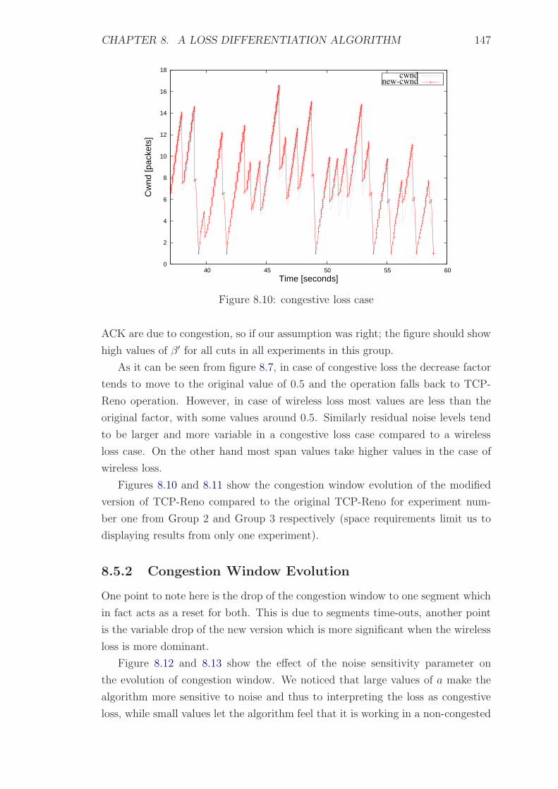
CHAPTER 8. A LOSS DIFFERENTIATION ALGORITHM 147
0
2
4
6
8
10
12
14
16
18
40 45 50 55 60
Cw
nd [p
acke
ts]
Time [seconds]
cwndnew-cwnd
Figure 8.10: congestive loss case
ACK are due to congestion, so if our assumption was right; the figure should show
high values of β ′ for all cuts in all experiments in this group.
As it can be seen from figure 8.7, in case of congestive loss the decrease factor
tends to move to the original value of 0.5 and the operation falls back to TCP-
Reno operation. However, in case of wireless loss most values are less than the
original factor, with some values around 0.5. Similarly residual noise levels tend
to be larger and more variable in a congestive loss case compared to a wireless
loss case. On the other hand most span values take higher values in the case of
wireless loss.
Figures 8.10 and 8.11 show the congestion window evolution of the modified
version of TCP-Reno compared to the original TCP-Reno for experiment num-
ber one from Group 2 and Group 3 respectively (space requirements limit us to
displaying results from only one experiment).
8.5.2 Congestion Window Evolution
One point to note here is the drop of the congestion window to one segment which
in fact acts as a reset for both. This is due to segments time-outs, another point
is the variable drop of the new version which is more significant when the wireless
loss is more dominant.
Figure 8.12 and 8.13 show the effect of the noise sensitivity parameter on
the evolution of congestion window. We noticed that large values of a make the
algorithm more sensitive to noise and thus to interpreting the loss as congestive
loss, while small values let the algorithm feel that it is working in a non-congested

CHAPTER 8. A LOSS DIFFERENTIATION ALGORITHM 148
0
5
10
15
20
25
30
35
40
45
50
40 45 50 55 60
Cw
nd [p
acke
ts]
Time [seconds]
cwndnew-cwnd
Figure 8.11: wireless loss case
0
10
20
30
40
50
60
0 10 20 30 40 50 60
Cw
nd [p
acke
ts]
Time [seconds]
cwndnew-cwnd
Figure 8.12: with noise sensitivity, a = 10, wireless loss case – Loss = 1.04483 %

CHAPTER 8. A LOSS DIFFERENTIATION ALGORITHM 149
0
10
20
30
40
50
60
0 10 20 30 40 50 60
Cw
nd [p
acke
ts]
Time [seconds]
cwndnew-cwnd
Figure 8.13: with noise sensitivity, a = 0.1, wireless loss case – Loss = 1.04483 %
lossy environment.
8.6 Summary
We presented a new technique for discriminating congestive packet drop from
non-congestive packet drop based on the noise level and span in out of order
PITs. The importance of this technique is that it is passive and can help TCP
congestion control algorithms in the judgement of congestion window reduction
when a packet drop happens. The technique can run along side other techniques
working to resolve the same problem and can help in taking the decision whenever
an ambiguity about the source of packet drop appears, for example; not all network
routers cooperate by setting the ECN bit(s). Also reverse traffic may affect delay-
based approaches. When such ambiguity appears, our technique can be consulted
especially if the network setup is similar to that mentioned in this chapter.
The approach that we proposed in this chapter is orthogonal to other ap-
proaches mentioned in literature, whether those which rely on queueing delay or
queue size or even network assisted techniques like ECN5. However; although it
has intersection with some of PIT-based techniques, we believe that the approach
is new and for this reason we provide a prolonged theoretical discussion of the
ideas and assumptions.
We suggested six general scenarios for evaluation of the new technique and
focused on one scenario where we mathematically formulated and proved the tech-
5Also uses average queue size.

CHAPTER 8. A LOSS DIFFERENTIATION ALGORITHM 150
nique. Finally we validated a non-implemented version in a controlled simulated
environment and showed that this technique can augment other available tech-
niques in helping TCP to differentiate between the two different types of packet
drop.

Chapter 9
Conclusions & Future Work
Most of the Internet protocols designs were influenced by the technologies which
existed at the time when the Internet was born. It was difficult at that time to
predict the evolution of technologies for the next decades. Since the birth of the In-
ternet, TCP, the most important Internet protocol that aims at providing reliable
data transfer, flow and congestion control has performed well. Its self-managed
congestion control algorithms preserve the stability of the Internet and the proto-
col has become the most used protocol for data transfer on the Internet. However,
the spread of new technologies such as fibre optics and wireless networks poses
many challenges to TCP in general and to TCP’s congestion control algorithms
in particular.
This dissertation focused on two main challenges to TCP congestion control.
The first challenge is link underutilisation when working in a high-speed long-delay
networks. Such networks are characterised by high bandwidth-delay product,
standard TCP congestion control algorithms have a problem utilising these pipes,
this is due to its fixed and small amount of congestion window increase per round
trip time, which is one packet per round trip time. The research community,
however; responded quickly in the last decade with a number of proposals in
the form of modular congestion control algorithms. Most of these proposals are
experimental and some of them have disadvantages and shortcomings. Therefore
this thesis makes two contributions which we believe that the congestion control
research community would benefit from: i) Improvements to one of the existing
algorithms (part of Linux kernel stack), show us through simulation that our
suggestions improves the responsiveness and aggressiveness shortcomings of this
algorithm. ii) TCP-Gentle, an incremental development over the latest proposed
algorithm (also part of Linux kernel stack) addressing this problem. Unlike all
other proposals, TCP-Gentle uses different increase rules depending on network
conditions. The thesis presents a throughput expression for the new algorithm
based on a deterministic model and shows through simulation and real test bed
151

CHAPTER 9. CONCLUSIONS & FUTURE WORK 152
experiments that the new algorithm is gentle to networks in the sense that it keeps
a small number of a TCP-Gentle flow packets in the queue compared to all other
TCP congestion control algorithms, it also has good fairness properties, nearly flat
rate in steady-state while at the same time maintains high responsiveness, high
link utilisation and friendliness to standard TCP. Therefore it is competitive to
existing algorithms.
The second challenge is the ability to differentiate between congestive loss and
non-congestive loss (e.g. wireless loss), this has been a problem for standard TCP
congestion control algorithms, since TCP makes a tacit assumption that each
packet loss is due to congestion and reduces its congestion window drastically.
The thesis proposes a novel loss differentiation algorithm which quantifies the
noise in packet inter arrival times and use this information together with the span
(ratio of maximum to minimum packet inter arrival times) to adapt the multiplica-
tive decrease factor according to a predefined logical formula. We show through
simulation experiments that in certain topologies the randomness in packet inter
arrival times and the span can be exploited to differentiate between the two types
of packet loss, to the best of our knowledge, this is a unique approach in packet
loss differentiation which is orthogonal to approaches mentioned in literature. The
thesis also suggestes that this algorithm can work cooperatively with other exist-
ing loss differentiation algorithms (especially in topologies were the algorithm is
efficient) and resolve any ambiguities that may arise in other algorithms.
On the modelling side of TCP congestion control, the thesis extends the well-
known drift model of TCP to account for wireless loss and some hypothetical
cases (e.g. variable multiplicative decrease). It shows us a stability analysis for
the new version of the model after linearising it around an equilibrium point. The
thesis mathematically shows how the wireless loss is considered disturbance and it
is beyond the control of standard TCP congestion control algorithms. Following
that, it analytically shows that this can be controlled via a variable multiplicative
decrease.
Because TCP protocol is still in use and technologies are evolving, there is a
potential for other problems to arise in future. There is also an interest to improve
the performance of networks (e.g. Multipath TCP). One part of our future work
is to investigate the performance of TCP algorithms in different network set-ups
including the Internet.
The thesis treated the end-to-end TCP congestion control approach. Despite
the advantages of this approach like scalability, ease of deployment, etc, there are
limitations for improvements, most work is done by end-hosts which try to infer
things about the network. One such limitation is the reverse path traffic which
affects ACK-based protocols that use estimates like delay and queue size based

CHAPTER 9. CONCLUSIONS & FUTURE WORK 153
on round trip time measurements as part of their congestion control algorithms.
TCP-Gentle is subject to this problem, however our argument against this is that
if the reverse traffic is persistent the algorithm is tricked and assumes a case of
congestion then takes a sequence of events which eventually leads to a fall back
to standard TCP congestion control algorithm operation, i.e. the worst case is to
work like the standard TCP congestion control algorithms (increase until a packet
loss happens then decrease).
Having said that, another part of our future work will focus more on network
assisted approaches hoping to investigate the limitations of totally depending on
end-hosts, interesting examples are: XCP protocol, lower layer QCN approach.
Performance evaluation and analysis of these are a of research interest.

References
[1] NS-2 TCP-Linux: an NS-2 TCP implementation with congestion control
algorithms from Linux (New York, NY, USA, 2006), ACM Press.
[2] A statistical method of packet loss type discrimination in wired-wireless net-
works (Jan. 2006), Consumer Communications and Networking Conference,
2006. CCNC 2006. 2006 3rd IEEE.
[3] Linux Foundation Website. http://www.linuxfoundation.org/
collaborate/workgroups/networking/tcp_testing#Congestion_
Control, May 2010.
[4] Performance of Quantized Congestion Notification in TCP Incast Scenarios
of Data Centers (Aug. 2010), The 18th Annual Meeting of the IEEE In-
ternational Symposium on Modeling, Analysis and Simulation of Computer
and Telecommunication Systems, MASCOTS.
[5] Allman, M., Paxson, V., and Stevens, W. TCP Congestion Con-
trol. RFC 2581 (Proposed Standard), Apr. 1999. Obsoleted by RFC 5681,
updated by RFC 3390.
[6] Altman, E., Avrachenkov, K., and Barakat, C. A stochastic model
of TCP/IP with stationary random losses. IEEE/ACM Trans. Netw. 13, 2
(2005), 356–369.
[7] Andersen, D. Carnegie Mellon University, Parallel Data Lab’s Current
Projects. http://www.pdl.cmu.edu/Incast/, Aug. 2010.
[8] Andrew, L. L. H., Low, S. H., and Wydrowski, B. P. Understanding
XCP: equilibrium and fairness. IEEE/ACM Trans. Netw. 17, 6 (2009), 1697–
1710.
[9] Baiocchi, A., Castellani, A., and Vacirca, F. YeAH-TCP: yet An-
other Highspeed TCP. In Fifth International Workshop on Protocols for
FAST Long-Distance Networks (PFLDnet-07) (February 2007), pp. 37–42.
154

REFERENCES 155
[10] Balakrishnan, H. Challenges to Reliable Data Transport over Heteroge-
neous Wireless Networks. PhD thesis, Computer Science Division University
of California, Berkeley, 1998.
[11] Bansal, D., and Balakrishnan, H. Binomial Congestion Control Al-
gorithms. In IEEE Infocom 2001 (Anchorage, AK, April 2001).
[12] Barakat, C., Altman, E., and Dabbous, W. On TCP performance
in an heterogeneous network: A survey. Tech. rep.
[13] Bertsekas, D. P. Nonlinear Programming, 1st ed. Athena Scientific, 1995.
[14] Biaz, S., and Vaidya, N. H. Discriminating congestion losses from wire-
less losses using inter-arrival times at the receiver. IEEE Symposium AS-
SET’99 (Mar. 1999), 10–17.
[15] Biaz, S., and Vaidya, N. H. “de-randomizing” congestion losses to im-
prove TCP performance over wired-wireless networks. IEEE/ACM Trans.
Netw. 13, 3 (2005), 596–608.
[16] Blanton, E., Allman, M., Fall, K., and Wang, L. A Conserva-
tive Selective Acknowledgment (SACK)-based Loss Recovery Algorithm for
TCP. RFC 3517 (Proposed Standard), Apr. 2003.
[17] Border, J., Kojo, M., Griner, J., Montenegro, G., and Shelby,
Z. Performance Enhancing Proxies Intended to Mitigate Link-Related
Degradations. RFC 3135 (Informational), June 2001.
[18] Braden, R. Requirements for internet hosts – communication layers. RFC
1122, Oct. 1989.
[19] Brakmo, L. S., O’Malley, S. W., and Peterson, L. L. TCP Vegas:
new techniques for congestion detection and avoidance. SIGCOMM Comput.
Commun. Rev. 24, 4 (1994), 24–35.
[20] Casetti, C., Gerla, M., Mascolo, S., Sanadidi, M. Y., and Wang,
R. TCP Westwood: end-to-end congestion control for wired/wireless net-
works. Wirel. Netw. 8, 5 (2002), 467–479.
[21] Cavendish, D., Gerla, M., and Mascolo, S. A control theoretical
approach to congestion control in packet networks. IEEE/ACM Trans. Netw.
12, 5 (2004), 893–906.

REFERENCES 156
[22] Cen, S., Cosman, P. C., and Voelker, G. M. End-to-end differen-
tiation of congestion and wireless losses. IEEE/ACM Trans. Netw. 11, 5
(2003), 703–717.
[23] Chen, Y., Griffith, R., Liu, J., Katz, R. H., and Joseph, A. D.
Understanding tcp incast throughput collapse in datacenter networks. In
WREN ’09: Proceedings of the 1st ACM workshop on Research on enterprise
networking (New York, NY, USA, 2009), ACM, pp. 73–82.
[24] Chiu, D., and Jain, R. Analysis of the increase and decrease algorithms
for congestion avoidance in computer networks. Comput. Netw. ISDN Syst.
17, 1 (June 1989), 1–14.
[25] Costin Raiciu, Damon Wischik, M. H. Practical congestion control
for multipath transport protocols. Tech. rep.
[26] Damon Wischik, M. H., and Braun, M. B. The resource pooling
principle. Online, July 2010.
[27] David X. Wei, Jin Cheng; Low, S. H., and Sanjay, H. FAST TCP:
motivation, architecture, algorithms, performance. IEEE/ACM Trans.
Netw. 14, 6 (2006), 1246–1259.
[28] de Oliveira, R., and Braun, T. A delay-based approach using fuzzy
logic to improve TCP error detection in ad hoc networks.
[29] Douglas Leith, Lachlan Andrew, T. Q., Shorten, R., and Lavi,
K. Experimental evaluation of delay/loss-based tcp congestion control al-
gorithms. In PFLDnet (2008).
[30] Floyd, S. Congestion Control Principles. RFC 2914 (Best Current Prac-
tice), Sept. 2000.
[31] Floyd, S. HighSpeed TCP for Large Congestion Windows. RFC 3649,
Dec. 2003.
[32] Floyd, S. HighSpeed TCP for Large Congestion Windows, Dec. 2003.
[33] Floyd, S. Limited Slow-Start for TCP with Large Congestion Windows.
RFC 3742 (Experimental), Mar. 2004.
[34] Floyd, S. Metrics for the evaluation of congestion control mechanisms.
RFC 5166, Mar. 2008.

REFERENCES 157
[35] Floyd, S., Allman, M., ICIR, Jain, A., Networks, F., Sarolahti,
P., and Center, N. R. Quick-start for tcp and ip. RFC 4782, Jan. 2007.
[36] Floyd, S., Handley, M., and Padhye, J. A comparison of equation-
based and aimd congestion control. Tech. rep., 2000.
[37] Floyd, S., Handley, M., Padhye, J., and Widmer, J. TCP Friendly
Rate Control (TFRC): Protocol Specification. RFC 5348 (Proposed Stan-
dard), Sept. 2008.
[38] Floyd, S., Henderson, T., and Gurtov, A. The NewReno Modifica-
tion to TCP’s Fast Recovery Algorithm. RFC 3782 (Proposed Standard),
Apr. 2004.
[39] Floyd, S., and Jacobson, V. Traffic phase effects in packet-switched
gateways. SIGCOMM Comput. Commun. Rev. 21, 2 (1991), 26–42.
[40] Floyd, S., and Kohler, E. Profile for Datagram Congestion Control
Protocol (DCCP) Congestion Control ID 2: TCP-like Congestion Control.
RFC 4341 (Proposed Standard), Mar. 2006.
[41] Floyd, S., Kohler, E., and Padhye, J. Profile for Datagram Conges-
tion Control Protocol (DCCP) Congestion Control ID 3: TCP-Friendly Rate
Control (TFRC). RFC 4342 (Proposed Standard), Mar. 2006. Updated by
RFC 5348.
[42] Floyd, S., Mahdavi, J., Mathis, M., and Podolsky, M. An Exten-
sion to the Selective Acknowledgement (SACK) Option for TCP. RFC 2883
(Proposed Standard), July 2000.
[43] Fomenkov, M., Keys, K., Moore, D., and Claffy, K. Longitu-
dinal study of internet traffic in 1998-2003. In WISICT ’04: Proceedings
of the winter international synposium on Information and communication
technologies (2004), Trinity College Dublin, pp. 1–6.
[44] Fu, C., and Liew, S. TCP Veno: TCP enhancement for transmission
over wireless access, 2003.
[45] Gevros, P., Crowcroft, J., Kirstein, P., and Bhatti, S. Conges-
tion control mechanisms and the best effort service model. IEEE Network
15 (2001), 16–26.
[46] H. Shimonishi, T. Hama, T. M. Tcp-adaptive reno: Improving efficiency-
friendliness tradeoffs of tcp congestion control algorithm. In PFLDnet
(2006).

REFERENCES 158
[47] Ha, S., Rhee, I., and Xu, L. Cubic: a new tcp-friendly high-speed tcp
variant. SIGOPS Oper. Syst. Rev. 42, 5 (2008), 64–74.
[48] Hacker, T. J., Noble, B. D., and Athey, B. D. Improving throughput
and maintaining fairness using parallel TCP. In IEEE InfoCom (2004).
[49] Hadrien Bullot, R. L. C., and Hughes-Jones, R. Evaluation of
advanced tcp stacks on fast long-distance production networks. Journal of
Grid Computing Volume 1, 4 (Dec. 2003), 345–359.
[50] Harrick, S. G. Extended analysis of binary adjustment algorithms. Tech.
rep., 2002.
[51] Hassan, M., and Jain, R. High Performance TCP/IP Networking, Con-
cepts, Issues, and Solutions. Pearson Education, Inc, 2004.
[52] Henderson, T. Http/1.0 traffic generator for ns-2. Online, 1998.
[53] Jain, R. The Art of Computer Systems Performance Analysis. John Wiley
& Sons, Inc., 1991.
[54] Jin, C., Wei, D. X., and Low, S. H. Fast tcp: Motivation, architecture,
algorithms, performance, 2004.
[55] Jin, S., Guo, L., Matta, I., and Bestavros, A. Tcp-friendly simd
congestion control and its convergence behavior. In in Proceedings of ICNP
(2001).
[56] Ka-Cheong Leung Li, V. Transmission control protocol TCP in wireless
networks: issues, approaches, and challenges. Communications Surveys &
Tutorials, IEEE 8, 4 (Fourth Quarter 2006), 64–79.
[57] Katabi, D. Decoupling Congestion Control and Bandwidth Allocation Poli-
cyWith Application to High Bandwidth-Delay Product Networks. PhD thesis,
Department of Electrical Engineering and Computer Science, M.I.T., Mar.
2003.
[58] Katabi, D., Handley, M., and Rohrs, C. Congestion control for high
bandwidth-delay product networks. SIGCOMM Comput. Commun. Rev.
32, 4 (October 2002), 89–102.
[59] Katti, S., Katabi, D., Blake, C., Kohler, E., and Strauss, J.
Multiq: automated detection of multiple bottleneck capacities along a path.
In IMC ’04: Proceedings of the 4th ACM SIGCOMM conference on Internet
measurement (New York, NY, USA, 2004), ACM, pp. 245–250.

REFERENCES 159
[60] Kelly, F., Maulloo, A., and Tan, D. Rate control for communication
networks: shadow prices, proportional fairness and stability. Journal of the
Operational Research Society 49, 3 (March 1998), 237–252.
[61] Kelly, T. Scalable TCP: Improving Performance in Highspeed Wide Area
Networks, Apr. 2003.
[62] Keshav, S. Congestion Control in Computer Networks. PhD thesis, UC
Berkeley, Sept. 1991.
[63] Kesselman, A., and Mansour, Y. Adaptive aimd congestion control.
Algorithmica Volume 43, 1-2 (Sept. 2005), 97–111.
[64] King, R., Baraniuk, R. G., and Riedi, R. H. TCP-Africa: an adaptive
and fair rapid increase rule for scalable TCP. In INFOCOM (2005), IEEE,
pp. 1838–1848.
[65] Kohler, E., Handley, M., and Floyd, S. Datagram Congestion Con-
trol Protocol (DCCP). RFC 4340 (Proposed Standard), Mar. 2006. Updated
by RFCs 5595, 5596.
[66] Lathi, B. Modern Digital and Analog Communication Systems, 3rd ed.
Oxford University Press, 1998.
[67] Leith, D., and Shorten, R. H-tcp: Tcp for high-speed and long-distance
networks. In in Proc. PFLDnet, Argonne (2004).
[68] Li, Y.-T., Leith, D., and Shorten, R. N. Experimental evaluation
of tcp protocols for high-speed networks. IEEE/ACM Trans. Netw. 15, 5
(2007), 1109–1122.
[69] Liu, S., Basar, T., and Srikant, R. TCP-Illinois: a loss and delay-
based congestion control algorithm for high-speed networks. In valuetools
’06: Proceedings of the 1st international conference on Performance evalua-
tion methodolgies and tools (New York, NY, USA, 2006), ACM, p. 55.
[70] Low, S. H. A duality model of tcp and queue management algorithms.
IEEE/ACM Trans. Netw. 11, 4 (2003), 525–536.
[71] Mathis, M., Mahdavi, J., Floyd, S., and Romanow, A. TCP Selec-
tive Acknowledgment Options. RFC 2018 (Proposed Standard), Oct. 1996.
[72] Mathis, M., Semke, J., and Mahdavi, J. The macroscopic behavior
of the TCP congestion avoidance algorithm. Computer Communications
Review 27, 3 (1997).

REFERENCES 160
[73] Miras, D., Bateman, M., and Bhatti, S. Fairness of High-Speed TCP
Stacks. Advanced Information Networking and Applications, International
Conference on 0 (2008), 84–92.
[74] Misra, V., Gong, W., and Towsley, D. Stochastic differential equation
modeling and analysis of TCP-windowsize behavior, 1999.
[75] Misra, V., Gong, W.-B., and Towsley, D. Fluid-based analysis of a
network of aqm routers supporting TCP flows with an application to red.
SIGCOMM Comput. Commun. Rev. 30, 4 (2000), 151–160.
[76] Nguyen, G. T., Noble, B., Katz, R. H., and Satyanarayanan,
M. A trace-based approach for modeling wireless channel behavior. In In
Proceedings of the Winter Simulation Conference (1996), pp. 597–604.
[77] Ogata, K. Modern Control Engineering, 3rd ed. Prentice Hall, Inc, 1997.
[78] Padhye, J., Firoiu, V., Towsley, D., and Krusoe, J. Modeling
TCP throughput:A simple model and its empirical validation. Proceedings
of the ACM SIGCOMM ’98 conference on Applications, technologies, archi-
tectures, and protocols for computer communication (1998), 303–314.
[79] Paxson, V. Measurements and Analysis of End-to-End Internet Dynamics.
PhD thesis, Computer Science Division University of California, Berkeley,
Apr. 1997.
[80] Postel, J. Transmission Control Protocol. RFC 793 (Standard), Sept.
1981. Updated by RFCs 1122, 3168.
[81] Ramakrishnan, K., Floyd, S., and Black, D. The Addition of Ex-
plicit Congestion Notification (ECN) to IP. RFC 3168 (Proposed Standard),
Sept. 2001.
[82] Ron Pan, Balaji Prabhakar, A. L. QCN:Quantized Con-
gestion Notification. www.stanford.edu/~balaji/presentations/
au-prabhakar-qcn-description.pdf, Aug. 2010.
[83] Saltzer, J. H., Reed, D. P., and Clark, D. D. End-To-End argu-
ments in system design. ACM Transactions on Computer Systems 2, 4 (Nov.
1984), 277–288.
[84] Samios, C. B., and Vernon, M. K. Modeling the throughput of TCP
Vegas. SIGMETRICS Perform. Eval. Rev. 31, 1 (2003), 71–81.

REFERENCES 161
[85] Sarolahti, P. TCP Performance in Heterogeneous Wireless Networks.
PhD thesis, Department of Computer Science, University of Helsinki, Fin-
land, 2007.
[86] Siekkinen, M. Measuring the internet, part 2 - digging in. University of
Oslo, Feb. 2007.
[87] Source, O. The network simulator - ns-2, Jan 2008.
http://www.isi.edu/nsnam/ns/.
[88] Srikant, R. The Mathematics of Internet Congestion Control. Birkhauser,
2004.
[89] Stevens, W. TCP Slow Start, Congestion Avoidance, Fast Retransmit,
and Fast Recovery Algorithms. RFC 2001 (Proposed Standard), Jan. 1997.
Obsoleted by RFC 2581.
[90] Stevens, W. R. TCP/IP illustrated (vol. 1): The Protocols. Addison-
Wesley Longman Publishing Co., Inc., Boston, MA, USA, 1994.
[91] Stewart, L., Armitage, G., and Huebner, A. Collateral damage: The
impact of optimised TCP variants on real-time traffic latency in consumer
broadband environments. In NETWORKING ’09: Proceedings of the 8th
International IFIP-TC 6 Networking Conference (Berlin, Heidelberg, 2009),
Springer-Verlag, pp. 392–403.
[92] Swan, T. GNU C++ FOR LINUX. Que Corporation, 1999.
[93] Tan, K., Song, J., Zhang, Q., and Sridharan, M. A compound TCP
approach for high-speed and long distance networks. Tech. Rep. MSR-TR-
2005-86, Microsoft Research, July 2005.
[94] Tanenbaum, A. S. Computer Networks, 4th ed. Pearson Education, Inc,
2003.
[95] Tobe, Y., Tamura, Y., Molano, A., Ghosh, S., and Tokuda, H.
Achieving moderate fairness for udp flows by path-status classification. In
LCN ’00: Proceedings of the 25th Annual IEEE Conference on Local Com-
puter Networks (Washington, DC, USA, 2000), IEEE Computer Society,
p. 252.
[96] V.Jacobson. Congestion avoidance and control. SIGCOMM’88 (Aug.
1988), 314–329.

REFERENCES 162
[97] Vojnovic, M., Le Boudec, J.-Y., and Boutremans, C. Global
fairness of additive-increase and multiplicative-decrease with heterogeneous
round-trip times. In IEEE INFOCOM‘2000 (2000), pp. 1303–1312.
[98] Wang, Z., and Crowcroft, J. A new congestion control scheme: slow
start and search (tri-s). SIGCOMM Comput. Commun. Rev. 21, 1 (1991),
32–43.
[99] Weigle, M. C., Sharma, P., and Iv, J. R. F. Iv. “performance of
competing high-speed tcp flows. In In the Proceedings of NETWORKING
(2006).
[100] Welzl, M. Network Congestion Control: Managing Internet Traffic (Wiley
Series on Communications Networking & Distributed Systems). John Wiley
& Sons, 2005.
[101] Wierman, A., Osogami, T., and Olsen, J. A unified framework for
modeling TCP-vegas, TCP-sack, and TCP-reno. In International Sympo-
sium on Modeling, Analysis, and Simulation of Computer and Telecommu-
nication Systems (Oct. 2003).
[102] Xu, L., Harfoush, K., and Rhee, I. Binary Increase Congestion Control
(BIC) for Fast Long-Distance Networks. In IEEE INFOCOM (March 2004),
vol. 4, pp. 2514–2524.
[103] Yang, Y. R., and Lam, S. S. General aimd congestion control. In ICNP
’00: Proceedings of the 2000 International Conference on Network Protocols
(Washington, DC, USA, 2000), IEEE Computer Society, p. 187.
[104] Ye, L., Wang, Z., Che, H., Chan, H. B. C., and Lagoa, C. M.
Utility function of tcp. Comput. Commun. 32, 5 (2009), 800–805.
[105] Zhang, G., Wu, Y., and Liu, Y. Stability and sensitivity for congestion
control in wireless networks with time varying link capacities. In ICNP
’05: Proceedings of the 13TH IEEE International Conference on Network
Protocols (Washington, DC, USA, 2005), IEEE Computer Society, pp. 401–
412.

Appendix A
History Time Line for
TCP-Related Issues
History Notes: TCP/IP and Transport Layer Protocols
Compiled by: Talal A.Edwan.
Date: 04-March-2008. Update date: 23-July-2010.
TCP/IP Overview and History1
The best place to start looking at TCP/IP is probably the name itself. TCP/IP
in fact consists of dozens of different protocols, but only a few are the main pro-
tocols that define the core operation of the suite. Of these key protocols, two are
usually considered the most important. The Internet Protocol (IP) is the primary
OSI network layer (layer three) protocol that provides addressing, datagram rout-
ing and other functions in an internetwork. The Transmission Control Protocol
(TCP) is the primary transport layer (layer four) protocol, and is responsible for
connection establishment and management and reliable data transport between
software processes on devices.
Due to the importance of these two protocols, their abbreviations have come to
represent the entire suite: TCP/IP. (In a moment we’ll discover exactly the
history of that name.) IP and TCP are important because many of TCP/IP’s
most critical functions are implemented at layers three and four. However, there
is much more to TCP/IP than just TCP and IP. The protocol suite as a whole
requires the work of many different protocols and technologies to make a functional
1This text is quoted from {source:http://www.tcpipguide.com/free/t TCPIPOverviewandHistory.htm}
163

APPENDIX A. HISTORY TIME LINE FOR TCP-RELATED ISSUES 164
network that can properly provide users with the applications they need.
TCP/IP uses its own four-layer architecture that corresponds roughly to the OSI
Reference Model and provides a framework for the various protocols that comprise
the suite. It also includes numerous high-level applications, some of which are well-
known by Internet users who may not realise they are part of TCP/IP, such as
HTTP (which runs the World Wide Web) and FTP. In the topics on TCP/IP
architecture and protocols I provide an overview of most of the important TCP/IP
protocols and how they fit together. Early TCP/IP History
As I said earlier, the Internet is a primary reason why TCP/IP is what it is today.
In fact, the Internet and TCP/IP are so closely related in their history that it is
difficult to discuss one without also talking about the other. They were developed
together, with TCP/IP providing the mechanism for implementing the Internet.
TCP/IP has over the years continued to evolve to meet the needs of the Internet
and also smaller, private networks that use the technology. I will provide a brief
summary of the history of TCP/IP here; of course, whole books have been written
on TCP/IP and Internet history, and this is a technical Guide and not a history
book, so remember that this is just a quick look for sake of interest.
The TCP/IP protocols were initially developed as part of the research network
developed by the United States Defence Advanced Research Projects Agency
(DARPA or ARPA). Initially, this fledgling network, called the ARPAnet, was
designed to use a number of protocols that had been adapted from existing tech-
nologies. However, they all had flaws or limitations, either in concept or in prac-
tical matters such as capacity, when used on the ARPAnet. The developers of the
new network recognised that trying to use these existing protocols might eventu-
ally lead to problems as the ARPAnet scaled to a larger size and was adapted for
newer uses and applications.
In 1973, development of a full-fledged system of inter networking protocols for the
ARPAnet began. What many people don’t realise is that in early versions of this
technology, there was only one core protocol: TCP. And in fact, these letters
didn’t even stand for what they do today; they were for the Transmission Control
Program. The first version of this predecessor of modern TCP was written in
1973, then revised and formally documented in RFC 675, Specification of Internet
Transmission Control Program, December 1974.
Modern TCP/IP Development and the Creation of TCP/IP Architecture:
Testing and development of TCP continued for several years. In March 1977,

APPENDIX A. HISTORY TIME LINE FOR TCP-RELATED ISSUES 165
version 2 of TCP was documented. In August 1977, a significant turning point
came in TCP/IPs development. Jon Postel, one of the most important pioneers
of the Internet and TCP/IP, published a set of comments on the state of TCP.
In that document (known as Internet Engineering Note number 2, or IEN 2), he
provided what I consider superb evidence that reference models and layers aren’t
just for textbooks, and really are important to understand:
“We are screwing up in our design of internet protocols by violating the principle
of layering. Specifically we are trying to use TCP to do two things: serve as a
host level end to end protocol, and to serve as an internet packaging and routing
protocol. These two things should be provided in a layered and modular way. I
suggest that a new distinct internetwork protocol is needed, and that TCP be used
strictly as a host level end to end protocol.”
– Jon Postel, IEN 2, 1977
What Postel was essentially saying was that the version of TCP created in the
mid-1970s was trying to do too much. Specifically, it was encompassing both layer
three and layer four activities (in terms of OSI Reference Model layer numbers).
His vision was prophetic, because we now know that having TCP handle all of
these activities would have indeed led to problems down the road.
Postel’s observation led to the creation of TCP/IP architecture, and the splitting
of TCP into TCP at the transport layer and IP at the network layer; thus the
name TCP/IP. (As an aside, it’s interesting, given this history, that sometimes
the entire TCP/IP suite is called just IP, even though TCP came first.) The
process of dividing TCP into two portions began in version 3 of TCP, written in
1978. The first formal standard for the versions of IP and TCP used in modern
networks (version 4) were created in 1980. This is why the first real version of IP is
version 4 and not version 1. TCP/IP quickly became the standard protocol set for
running the ARPAnet. In the 1980s, more and more machines and networks were
connected to the evolving ARPAnet using TCP/IP protocols, and the TCP/IP
Internet was born.
Key Concept: TCP/IP was initially developed in the 1970s as part of an effort to
define a set of technologies to operate the fledgling Internet. The name TCP/IP
came about when the original Transmission Control Program (TCP) was split
into the Transmission Control Protocol (TCP) and Internet Protocol (IP). The
first modern versions of these two key protocols were documented in 1980 as TCP
version 4 and IP version 4.
Important Factors in the Success of TCP/IP:

APPENDIX A. HISTORY TIME LINE FOR TCP-RELATED ISSUES 166
TCP/IP was at one time just one of many different sets of protocols that could
be used to provide network-layer and transport-layer functionality. Today there
are still other options for inter networking protocol suites, but TCP/IP is the
universally-accepted world-wide standard. Its growth in popularity has been due
to a number of important factors. Some of these are historical, such as the fact
that it is tied to the Internet as described above, while others are related to the
characteristics of the protocol suite itself. Chief among these are the following:
- Integrated Addressing System: TCP/IP includes within it (as part of the Internet
Protocol, primarily) a system for identifying and addressing devices on both small
and large networks. The addressing system is designed to allow devices to be
addressed regardless of the lower-level details of how each constituent network is
constructed. Over time, the mechanisms for addressing in TCP/IP have improved,
to meet the needs of growing networks, especially the Internet. The addressing
system also includes a centralised administration capability for the Internet, to
ensure that each device has a unique address.
- Design For Routing: Unlike some network-layer protocols, TCP/IP is specifi-
cally designed to facilitate the routing of information over a network of arbitrary
complexity. In fact, TCP/IP is conceptually concerned more with the connection
of networks, than with the connection of devices. TCP/IP routers enable data to
be delivered between devices on different networks by moving it one step at a time
from one network to the next. A number of support protocols are also included in
TCP/IP to allow routers to exchange critical information and manage the efficient
flow of information from one network to another.
- Underlying Network Independence: TCP/IP operates primarily at layers three
and above, and includes provisions to allow it to function on almost any lower-
layer technology, including LANs, wireless LANs and WANs of various sorts. This
flexibility means that one can mix and match a variety of different underlying
networks and connect them all using TCP/IP.
- Scalability: One of the most amazing characteristics of TCP/IP is how scal-
able its protocols have proven to be. Over the decades it has proven its mettle
as the Internet has grown from a small network with just a few machines to a
huge internetwork with millions of hosts. While some changes have been required
periodically to support this growth, these changes have taken place as part of the
TCP/IP development process, and the core of TCP/IP is basically the same as it
was 25 years ago.
- Open Standards and Development Process: The TCP/IP standards are not
proprietary, but open standards freely available to the public. Furthermore, the

APPENDIX A. HISTORY TIME LINE FOR TCP-RELATED ISSUES 167
process used to develop TCP/IP standards is also completely open. TCP/IP
standards and protocols are developed and modified using the unique, democratic
RFC process, with all interested parties invited to participate. This ensures that
anyone with an interest in the TCP/IP protocols is given a chance to provide
input into their development, and also ensures the world-wide acceptance of the
protocol suite.
- Universality: Everyone uses TCP/IP because everyone uses it!
This last point is, perhaps ironically, arguably the most important. Not only is
TCP/IP the underlying language of the Internet, it is also used in most private
networks today. Even former competitors to TCP/IP such as NetWare now use
TCP/IP to carry traffic. The Internet continues to grow, and so do the capabilities
and functions of TCP/IP. Preparation for the future continues, with the move
to the new IP version 6 protocol in its early stages. It is likely that TCP/IP will
remain a big part of inter networking for the foreseeable future.
Key Concept: While TCP/IP is not the only inter networking protocol suite, it
is definitely the most important one. Its unparalleled success is due to a wide
variety of factors. These include its technical features, such as its routing-friendly
design and scalability, its historical role as the protocol suite of the Internet, and
its open standards and development process, which reduce barriers to acceptance
of TCP/IP protocols.
For Brief History of Wireless Technologies see: Wireless Data Technologies. Vern
A. Dubendorf 2003 John Wiley & Sons, Ltd ISBN: 0-470-84949-5. Notice that in
802.11(b) are popular in 2000.
Note: the aim of the following history time line is to:
• See the effect of various telecommunication technologies (e.g. wireless, long
fat pipes,. . . ) on the evolution of transport layer reliable protocols. (trend
of research).
• Show the need for reliable protocols (the topic is still evolving).
• Help in tracking the changes and learning from previous algorithms.
• Provide short reading list for certain topics. (organised research or pointers
for research papers).

APPENDIX A. HISTORY TIME LINE FOR TCP-RELATED ISSUES 168
1957: USSR launches Sputnik, first artificial earth satellite. The start of global
telecommunications. Satellites play an important role in transmitting all sorts
of data today. In response, US forms the Advanced Research Projects Agency
(ARPA) within the Department of Defence (DOD) to establish US lead in science
and technology applicable to the military. {source: Gromov’s Timeline, inthistory
file}
1967: ARPANET design discussions held by Larry Roberts at ARPA IPTO PI
meeting in Ann Arbor, Michigan (April)
ACM Symposium on Operating Systems Principles in Gatlinburg, Tennessee (Oc-
tober).
- First design paper on ARPANET published by Larry Roberts: ”Multiple Com-
puter Networks and Inter computer Communication.
- First meeting of the three independent packet network teams (RAND, NPL,
ARPA).
National Physical Laboratory (NPL) in Middlesex, England develops NPL Data
Network under Donald Watts Davies who coins the term packet. The NPL net-
work, an experiment in packet-switching, used 768kbps lines.
1969: Birth of Internet. ARPANET commissioned by DOD (US Dept. of Defence)
for research into networking. First node at UCLA (Los Angeles) closely followed
by nodes at Stanford Research Institute, UCSB (Santa Barbara) and U of Utah
(4 Nodes) {source: Gromov’s Timeline, inthistory file}
1970: ALOHANET developed at the University of Hawaii. {source: Gromov’s
Timeline, inthistory file}
1971: People communicate over a network. 15 nodes (23 hosts) on ARPANET.
E-mail invented.
{source: Gromov’s Timeline, inthistory file}
1970-1973: The ARPANET was a success from the very beginning.
1973: Need of development of fully fledged system for ARPAnet.
1974: TCP v.1, Vint Cerf and Bob Kahn publish ”A Protocol for Packet Network
Interconnection” which specified in detail the design of a Transmission Control
Program (TCP). {IEEE Trans Comm} BBN opens Telenet, the first public packet
data service (a commercial version of ARPANET).
Formally documented in RFC 675 December 1974.

APPENDIX A. HISTORY TIME LINE FOR TCP-RELATED ISSUES 169
1976: Elizabeth II, Queen of the United Kingdom sends out an email on 26 March
from the Royal Signals and Radar Establishment (RSRE) in Malvern.
UUCP (Unix-to-Unix CoPy) developed at AT&T Bell Labs and distributed with
UNIX one year later.
1977: March, TCP v.2 was documented.
August, TCP v.2 should be split into two protocols. According to Jon Postel, IEN
2
1978: TCP v.3, The process of dividing TCP into two portions began in version
3 of TCP and it was written.
1980: User Datagram Protocol (UDP) created by David P. Reed.
1980: TCP v.4, first formal standard for the versions of IP and TCP used in mod-
ern networks.
January, RFC 760 761 outline new specifications for the two protocols IP and
TCP. {source: www.cs.utexas.edu}February, RFC TCP/IP becomes the preferred military protocol. {source: www.cs.utexas.edu}TCP/IP Internet was born.
1981: September, IETF RFC 793 (TCP), RFC 791 (IP). RFC-791 replaced RFC-
760.
1981: Jerome H. Saltzer, David P. Reed, and David D. Clark, s.l. End-to-End
Arguments in System Design. IEEE Computer Society, 1981, Proceedings of the
2nd International Conference on Distributed Computing Systems, Paris, 1981, pp.
509-512.
Jerome H. Saltzer, David P. Reed, and David D. Clark. End-to-end arguments in
system design. ACM Transactions on Computer Systems 2, 4 (November 1984)
pages 277-288. An earlier version appeared in the Second International Conference
on Distributed Computing Systems (April, 1981) pages 509-512.
{source: wikipedia, End-to-end principle}
1982: The term ‘Internet’ was used for the first time. {source: Gromov’s Timeline,
inthistory file}
1983: 4.2BSD, Many of the implementations of TCP/IP at the time (1973-1980)
were pulled together to create the first widely available (and used) version of
TCP/IP. {source: node8 file}.
1984: Domain Name System (DNS) introduced.
-Number of hosts breaks 1,000.

APPENDIX A. HISTORY TIME LINE FOR TCP-RELATED ISSUES 170
-JUNET (Japan Unix Network) established using UUCP.
-JANET (Joint Academic Network) established in the UK using the Coloured
Book protocols; previously SERCnet.
1986: In October of ’86, the Internet had the first of what became a series of ‘con-
gestion collapses’. During this period, the data throughput from LBL (Lawrence
Berkeley Laboratories) to UC Berkeley (sites separated by 400 yards and two
IMP (Infrastructure Message Processor, i.e router) hops) dropped from 32 Kbps
to 40bps. This sudden factor-of-thousand drop in bandwidth embarked on an in-
vestigation of why things had gotten so bad. In particular, we wondered if the
4.3bsd (Berkeley UNIX) TCP was mis-behaving or if it could be tuned to work
better under abysmal network conditions. The answer to both of these questions
was “yes”.
1987: Karn’s Algorithm: P. Karn and C. Partridge. Improving Round-Trip Time
Estimates in Reliable Transport Protocols. Computer Communication Review,
17(5), August 1987.
1988: 4.3BSD TAHOE TCP
The Tahoe implementation of TCP (1988) introduced significant improvements
for working over a shared network (leading in 1989 to the Net/1 release). An al-
gorithm (Slow Start (congestion control) and multiplicative decrease (congestion
avoidance)) was introduce to control transmission following any detected conges-
tion. Under this algorithm, a TCP transmitter is allowed to transmit a number
of bytes determined by the smallest value of the window advertised by the re-
ceiver and a congestion window (cwnd). The cwnd is initially assigned a value of
1 segment, and is doubled following receipt of each ACK, normally resulting in
exponential window growth.
The algorithm also uses a variable to keep the threshold value of the send window
(ssthresh), which is initialised to the receiver’s advertised window size. Following
a retransmission time out, the algorithm assigns half of the current window to
ssthresh (this is the multiplicative decrease part of the algorithm), the cwnd is set
to one packet and the slow start phase begins. The cwnd is increased by one seg-
ment whenever an acknowledgement is received, until it reaches the ssthresh. At
this point, the algorithm switches to the congestion avoidance phase and the win-
dow size is only increased by a fraction of the segment (equivalent to an increment
of one segment per round trip delay).
The Fast Retransmission {RFC 2001} algorithm was also implemented into avoid
waiting for the retransmission timer to expire following every packet loss. In this

APPENDIX A. HISTORY TIME LINE FOR TCP-RELATED ISSUES 171
algorithm, a receiver sends a duplicate ACK immediately on reception of each
out of sequence packet. The transmitter interprets reception of 3 duplicate ACKs
(sufficient to avoid spurious retransmissions due to reordering of segments) as a
congestion packet loss and triggers the Slow Start algorithm.
1989: NET/1 TCP
1989: XTP
Xpress Transport Protocol (XTP) is a transport layer protocol for high-speed
networks promoted by the XTP Forum developed to replace TCP. XTP pro-
vides protocol options for error control, flow control, and rate control. Instead
of separate protocols for each type of communication, XTP controls packet ex-
change patterns to produce different models, e.g. reliable datagrams, transactions,
unreliable streams, and reliable multicast connections. XTP does not employ con-
gestion avoidance algorithms. XTP is a real-time option at Layer 4 for the US
Navy SAFENET LAN Profile.
”XTP Protocol Definition Revision 3.4”, Protocol Engines, Incorporated, 1900
State Street, Suite D, Santa Barbara, California 93101, 1989.
{source:http://en.wikipedia.org/wiki/Xpress Transport Protocol +
http://www.cs.virginia.edu/papers/p67-sanders.pdf}
1990: 4.4BSD RENO TCP
Reno TCP (1990, followed by Net/2 in 1991) introduced a further optimisation
(Fast Recovery) to improve performance following retransmission. When the third
duplicate ACK is received, the Reno TCP transmitter sets ssthresh to one half of
the current congestion window (cwnd) and retransmits the missing segment. The
cwnd is then set to ssthresh plus three segments (one segment per each duplicate
ACK that has already received). cwnd is then increased by one segment on re-
ception of each duplicate ACK which continues to arrive after fast-retransmission.
This allows the transmitter to send new data when cwnd is increased beyond the
value of the cwnd before the fast-retransmission. When an ACK arrives which
acknowledges all outstanding data sent before the duplicate ACKs were received,
the cwnd is set to ssthresh so that the transmitter slows down the transmission
rate and enters the linear increase phase.
Much had also been learned through research into alternative protocols to TCP
(e.g. XTP, NetBLT). This experience was transferred to TCP through the addi-
tion of ”header prediction”, providing a very significant performance improvement.

APPENDIX A. HISTORY TIME LINE FOR TCP-RELATED ISSUES 172
1991: Tri-S, a congestion control algorithm.
1992: T/TCP
TCP for Transactions,
RFC 1379: Braden, R. T., Extending TCP for Transactions-Concepts, 38 pages,
Nov. 1992.
RFC 1644: Braden, R. T., T/TCP-TCP Extensions for Transactions, Functional
Specification, 38 pages, July 1994.
{source: http://www.kohala.com/start/ttcp.html}.
1993: 4.4BSD NET/3 TCP
The 4.4 BSD release (1993) lead to Net/3 TCP, which continues to be one of the
reference implementations used by developers. This added capability for multi-
cast, long fat network extensions and various other refinements.
1993: Floyd, S., and Jacobson, V., Random Early Detection gateways for Con-
gestion Avoidance V.1 N.4, August 1993, p. 397-413. This is the basic paper that
describes RED queue management.
1994: VEGAS TCP
An experimental modification to TCP was proposed by Lawrence Brakmo at Uni-
versity of Arizona. This primarily added rate control to avoid congestion (rather
than react after detection of congestion) it emphasises packet delay, rather than
packet loss, as a signal to help determine the rate at which to send packets. Vegas
has not been widely implemented and is not universally accepted by the Internet
community and is still a subject of much controversy.
{source: wikipedia + see SIGCOMM94 paper}.
1994: T-TCP
T/TCP (Transactional TCP) is a variant of the TCP protocol. It is an experimen-
tal TCP extension for efficient transaction-oriented (request/response) service. It
was developed to fill the gap between TCP and UDP, by Bob Braden in 1994. Its
definition can be found in RFC 1644.
This protocol is faster than TCP and delivery reliability is comparable to that of
TCP. Unfortunately, T/TCP suffers from a major spoofing problem pointed out
by Vasim Valejev in 1998 in a posting to Bugtraq, and has not gained widespread
popularity.

APPENDIX A. HISTORY TIME LINE FOR TCP-RELATED ISSUES 173
{source: http://en.wikipedia.org/wiki/Category:Transport layer protocols}
1995: I-TCP
I-TCP: indirect TCP for mobile hosts
Abstract: IP based solutions to accommodate mobile hosts within existing in-
ternetworks do not address the distinctive features of wireless mobile computing.
IP-based transport protocols thus suffer from poor performance when a mobile
host communicates with a host on the fixed network. This is caused by frequent
disruptions in network layer connectivity due to - i) mobility and ii) unreliable
nature of the wireless link. We describe I-TCP, which is an indirect transport
layer protocol for mobile hosts. I-TCP utilizes the resources of Mobility Support
Routers (MSRs) to provide transport layer communication between mobile hosts
and hosts on the fixed network. With I-TCP, the problems related to mobility
and unreliability of wireless link are handled entirely within the wireless link; the
TCP/IP software on the fixed hosts is not modified. Using I-TCP on our testbed,
the throughput between a fixed host and a mobile host improved substantially in
comparison to regular TCP.
{source: http://citeseer.ist.psu.edu/bakre95itcp.html}
1995-1996: NEW-RENO TCP
Janey Hoe (of MIT) proposed a modification to Reno TCP usually called New-
Reno, which addressed two problems in TCP, these ideas are gradually finding
acceptance within the IETF. Hoe noted that a smaller value for ssthresh causes
premature termination of the slow start phase and subsequent slow increase of the
cwnd (i.e. the linear increase phase). A larger value causes the sender to over-feed
packets to the network (i.e. transmit too long a burst of data packets) causing
congestion. Since most TCP sessions last only for a short period of time, the
initial slow start period is significant for the over all performance.
Hoe proposed a method to estimate an optimum ssthresh value by calculating the
byte equivalent of bandwidth delay product of the network, when a new connection
is made. The bandwidth is calculated using the Packet-Pair algorithm (measuring
the arrival time of closely spaced ACKs at the sender).
If two or more segments have been lost from the transmitted data (window), the
Fast Retransmission and Fast Recovery algorithms will not be able to recover
the losses without waiting for retransmission time out. New-Reno overcomes this
problem by introducing the concept of a Fast Retransmission Phase, which starts
on detection of a packet loss (receiving 3 duplicate ACKs) and ends when the
receiver acknowledges reception of all data transmitted at the start of the Fast

APPENDIX A. HISTORY TIME LINE FOR TCP-RELATED ISSUES 174
Retransmission phase. If more than one packet is missing within the same window,
a retransmission only recovers the first lost packet from the window. The receiver
then ACKs reception of the retransmitted segment and all following segments up
to the next lost segment. This ACK is called a ”partial ACK”, because it has not
ACKed all the packets which were transmitted prior to the start of the current
Fast Retransmission Phase.
The transmitter assumes reception of a partial ACK during the Fast Retransmis-
sion phase as an indication that another packet has been lost within the window
and retransmits that packet immediately to prevent expiry of the retransmission
timer. New Reno sets the cwnd to one segment on reception of 3 duplicate ACKs
(i.e. when entering the Fast Retransmission Phase) and unacknowledged data are
retransmitted using the Slow Start algorithm. The transmitter is also allowed to
transmit a new data packet on receiving 2 duplicate ACKs. While the transmitter
is in the Fast Retransmission Phase, it continues to retransmit packets using Slow
Start until all packets have been recovered (without starting a new retransmis-
sion phase for partial ACKs). Although this modification may cause unnecessary
retransmissions, it reduces transmitter time outs and efficiently recovers multiple
packet loss using partial ACKs.
{source: tcp-evol file + RFC 2582}
1995-1996: Snoop TCP
The Snoop protocol is a TCP-aware link layer protocol designed to improve the
performance of TCP over networks of wired and single-hop wireless links. (Note:
The TCP split approach was before this work - mid 1990s-, see the background
part of [10], section 2.5.3 Split connection protocols).
{source: http://nms.lcs.mit.edu/ hari/papers/snoop.html}
1996: RTP
The Real-time Transport Protocol (or RTP) defines a standardised packet format
for delivering audio and video over the Internet. It was developed by the Audio-
Video Transport Working Group of the IETF and first published in 1996 as RFC
1889 which was made obsolete in 2003 by RFC 3550. {source: wikipedia}
Note: Call setup and tear-down for VoIP applications is usually performed by
either SIP (Session Initiation Protocol an application-layer control) or H.323 (an
ITU Telecommunication Standardisation Sector (ITU-T) standard ) protocols,
SIP is designed to be independent of the underlying transport layer; it can run on
TCP, UDP, or SCTP.
1996-1998: SELECTIVE ACKNOWLEDGEMENT OPTION (SACK)

APPENDIX A. HISTORY TIME LINE FOR TCP-RELATED ISSUES 175
The probability of multiple packet loss in a window is much greater for a long
fast network, where more packets are in flight. Although TCP is able to recover-
ing multiple packet losses without waiting for expiry of the retransmission timer,
frequent packet loss may still not be efficiently recovered. The SACK extension
(1996-98) improves TCP performance over such a network, and has been included
in some recent TCP implementations.
The SACK option is triggered when the receiver buffer holds in-sequence data
segments following a packet loss. The receiver then sends duplicate ACKs bearing
the SACK option to inform the transmitter which segments have been correctly
received. When the third duplicate ACKis received, a SACK TCP transmitter
retransmits only the missing packets starting with the sequence number acknowl-
edged by the duplicate ACKs, and followed by any subsequent unacknowledged
segments. The Fast Retransmission and Recovery algorithms are also modified
to avoid retransmitting already SACKed segments. The explicit information car-
ried by SACKs enables the transmitter to also accurately estimate the number of
transmitted data packets that have left the network (this procedure is known as
Forward Acknowledgement (FACK)), allowing transmission of new data to con-
tinue during retransmission. The SACK option is able to sustain high throughput
over a network subject to high packet loss and is therefore desirable for bulk trans-
fers over a DVB network. Optimisation of the algorithms which govern use of the
SACK information are still the subject of research, however the basic algorithms
are now widely implemented.
N Samaweera & G Fairhurst have proposed a refinement to SACK to solve the re-
liance of SACK on protocol timers when a retransmission is unsuccessful. {source:
tcp-evol file}
1997: RSVP
The Resource ReSerVation Protocol (RSVP), version 1 is described in RFC 2205,
is a Transport layer protocol designed to reserve resources across a network for
an integrated services Internet. ”RSVP does not transport application data but
is rather an Internet control protocol, like ICMP, IGMP, or routing protocols” -
RFC 2205.
{source wikipedia + http://www.isi.edu/div7/rsvp/rsvp.html}
1997: M-TCP
http://web.cecs.pdx.edu/ singh/mtcp.html
http://www.cs.pdx.edu/ singh/ftp/mtcp.ps.gz
Kevin Brown and Suresh Singh, M-TCP: TCP for Mobile Cellular Networks, ACM

APPENDIX A. HISTORY TIME LINE FOR TCP-RELATED ISSUES 176
CCR Vol. 27(5), 1997
1998: IPv6 RFC 2460.
1999: WTCP
WTCP (Wireless Transmission Control Protocol) is a proxy based modification of
TCP that preserves the end-to-end semantics of TCP. As its name suggests, it is
used in wireless networks to improve the performance of TCP.
{source: http://en.wikipedia.org/wiki/WTCP +
http://timely.crhc.uiuc.edu/Projects/wtcp/wtcp.html}
2000: SCTP
Stream Control Transmission Protocol standard draft document ( RFC2960 ) in
October 2000 (This RFC Updated by RFC 3309 and obsoleted by RFC 4960).
{source: wikipedia + http://tdrwww.exp-math.uni-essen.de/inhalt/
forschung/sctp fb/sctp intro.html}
2000: RFC 2914 Congestion Control Principles.
2000: TCP Westwood
TCP Westwood: Handling Dynamic Large Leaky Pipes
TCP Westwood (TCPW), is a sender-side-only modification to TCP NewReno
that is intended to better handle large bandwidth-delay product paths (large
pipes), with potential packet loss due to transmission or other errors (leaky pipes),
and with dynamic load (dynamic pipes).
TCPW relies on mining the ACK stream for information to help it better set the
congestion control parameters: Slow Start Threshold (ssthresh), and Congestion
Window (cwin). In TCPW, an ”Eligible Rate” is estimated and used by the
sender to update ssthresh and cwin upon loss indication, or during its ”Agile
Probing” phase, a proposed modification to the well-known Slow Start phase. In
addition, a scheme called Persistent Non Congestion Detection (PNCD) has been
devised to detect persistent lack of congestion and induce an Agile Probing phase
to expeditiously utilise large dynamic bandwidth.
The resultant performance gains in efficiency, without undue sacrifice of fairness,
friendliness, and stability have been reported in numerous papers that can be
found on this web site. Significant efficiency gains can be obtained for large leaky
dynamic pipes, while maintaining fairness. Under a more appropriate criterion for
friendliness, i.e. ”opportunistic friendliness”, TCPW is shown to have good, and

APPENDIX A. HISTORY TIME LINE FOR TCP-RELATED ISSUES 177
controllable, friendliness.
{source: Westwood Homepage, http://www.cs.ucla.edu/NRL/hpi/tcpw/ TCP }
2001: TCP Westwood+2
TCP Westwood+ is a sender-side only modification of the TCP Reno/NewReno
classic congestion control protocol stack that optimises the performance of TCP
congestion control especially over wireless networks. TCPW is based on end-to-
end bandwidth estimation to set congestion window and slow start threshold after
a congestion episode, that is, after three duplicate acknowledgements or a timeout.
The bandwidth is estimated by properly low-pass filtering the rate of returning
acknowledgement packets. The rationale of this strategy is simple: in contrast
with TCP Reno, which blindly halves the congestion window after three duplicate
ACKs, TCP Westwood+ adaptively sets a slow start threshold and a congestion
window which takes into account the bandwidth used at the time congestion is
experienced. TCP Westwood significantly increases fairness with respect to TCP
(New) Reno in wired networks and throughput over wireless links.
{source: Westwood Homepage, http://www.cs.ucla.edu/NRL/hpi/tcpw/ TCP }
2001: ATCP
ATCP: TCP for mobile ad hoc networks Liu, J.; Singh, S. Selected Areas in Com-
munications, IEEE Journal on Volume 19, Issue 7, Jul 2001 Page(s):1300 - 1315
Digital Object Identifier 10.1109/49.932698 Summary:Transport connections set
up in wireless ad hoc networks are plagued by problems such as high bit error
rates, frequent route changes, and partitions. If we run the transmission control
protocol (TCP) over such connections, the throughput of the connection is ob-
served to be extremely poor because TCP treats lost or delayed acknowledgments
as congestion. We present an approach where we implement a thin layer between
Internet protocol and standard TCP that corrects these problems and maintains
high end-to-end TCP throughput. We have implemented our protocol in FreeBSD,
and we present results from extensive experimentation done in an ad hoc network.
We show that our solution improves the TCP’s throughput by a factor of 2-3
2001: TCP HACK
R.K.Balan, B.P.Lee and K.R.R.Kumar ” TCP HACK: TCP Header checksum
option to Improve performance over Lossy Links ”, in proc. INFOCOM ’2001,
Anchorage, AK, pp.309-318.
2Also begining of Veno

APPENDIX A. HISTORY TIME LINE FOR TCP-RELATED ISSUES 178
2001: TCP-Real
TCP-real: improving real-time capabilities of TCP over heterogeneous networks.
Source:International Workshop on Network and Operating System Support for
Digital Audio and Video archive Proceedings of the 11th international workshop
on Network and operating systems support for digital audio and video table of
contents Port Jefferson, New York, United States Pages: 189 - 198 Year of Publi-
cation: 2001 ISBN:1-58113-370-7
Authors: C. Zhang College of Computer Science, Northeastern University, Boston,
MA V. Tsaoussidis College of Computer Science, Northeastern University, Boston,
MA
Abstract
We present a TCP-compatible and -friendly protocol which abolishes three major
shortfalls of TCP for reliable multimedia applications over heterogeneous net-
works: (i) ineffective bandwidth utilisation, (ii) unnecessary congestion-oriented
responses to wireless link errors (e.g., fading channels) and operations (e.g. hand-
offs), and (iii) wasteful window adjustments over asymmetric, low-bandwidth re-
verse paths. We propose TCP-Real, a high-throughput transport protocol that
minimises transmission-rate gaps, thereby enabling better performance and rea-
sonable playback timers. In TCP-Real, the receiver decides with better accuracy
about the appropriate size of the congestion window. Slow Start and timeout ad-
justments are used whenever congestion avoidance fails; however, rate and timeout
adjustments are cancelled whenever the receiving rate indicates sufficient avail-
ability of bandwidth. We detail the protocol design and we report significant
improvement on the performance of the protocol with time-constrained traffic,
wireless link errors and asymmetric paths.
{source: http://portal.acm.org/citation.cfm?id=378371}
2001-2002: HighSpeed TCP (HSTCP) is a new congestion control algorithm pro-
tocol defined in RFC 3649 for TCP (Sally Floyd).
{source: wikipedia + http://www.icir.org/floyd/hstcp.html}
2002: XCP The eXplicit Control Protocol
SIGCOMM02: http://www.acm.org/sigcomm/sigcomm2002/papers/xcp.pdf
{source: http://www.isi.edu/isi-xcp/}
2002: TCP Nice
TCP Nice, Arun Venkataramani, Ravi Kokku, and Mike Dahlin, 2002.

APPENDIX A. HISTORY TIME LINE FOR TCP-RELATED ISSUES 179
“makes good use of the spare bandwidth without affecting the traffic already
present.”
{source: http://www.cs.utexas.edu/users/arun/nice/ and link (2) at the end }
2003: TCP Veno
TCP Veno is a novel end-to-end congestion control scheme which can improve
TCP performance quite significantly over heterogeneous networks, particularly
when wireless links form part of such networks. The key innovation in Veno is the
enhancement of Reno congestion control algorithm by using the estimated state of
a connection based on Vegas. This scheme significantly reduces ”blind” reduction
of TCP window regardless of the cause of packet loss. The salient feature of TCP
Veno is that it only needs simple modification at sender side of Reno protocol
stack. Considering practical issues deployability and compatibility (conformance
with legacy connections), Veno TCP may be quickly deployed in ”hot” Mobile
Internet industry.
{source: www.ntu.edu.sg/home/ascpfu/veno/index.html}
2003: TCP Hybla
TCP Hybla is a experimental TCP enhancement conceived with the primary aim
of counteracting the performance deterioration caused by the long RTTs typical
of satellite connections. It consists of a set of procedures which includes, among
others:
- an enhancement of the standard congestion control algorithm (to grant long RTT
connections the same instantaneous segment transmission rate of a comparatively
fast reference connection).
- the mandatory adoption of the SACK policy.
- the use of timestamps.
- the adoption of Hoes channel bandwidth estimate.
- the implementation of packet spacing techniques (also known as ”pacing”).
TCP Hybla involves only sender-side modification of TCP. As that, it is fully
compatible with standard receivers.
{source: TCP Hybla Homepage, http://hybla.deis.unibo.it/}
2003: TCP-LP TCP Low Priority
Service prioritisation among different traffic classes is an important goal for the
future Internet. Conventional approaches to solving this problem consider the
existing best-effort class as the low-priority class, and attempt to develop mech-
anisms that provide “better-than-best-effort” service. We explore the opposite
approach, and devise a new distributed algorithm to realise a low-priority service

APPENDIX A. HISTORY TIME LINE FOR TCP-RELATED ISSUES 180
(as compared to the existing best effort) from the network endpoints. To this end,
we develop TCP Low Priority (TCP-LP), a distributed algorithm whose goal is
to utilise only the excess network bandwidth as compared to the “fair share” of
bandwidth as targeted by TCP. The key mechanisms unique to TCP-LP conges-
tion control are the use of one-way packet delays for congestion indications and
a TCP-transparent congestion avoidance policy. On the other hand, HSTCP-LP
(High-Speed TCP Low Priority) is an advanced TCP version targeted towards
fast long-distance networks (i.e., networks operating at 622 Mb/s, 2.5 Gb/s, or
10 Gb/s and spanning several countries or states). HSTCP-LP is a TCP-LP ver-
sion with aggressive window increase policy. More details on HSTCP-LP could be
found below. {source: http://www.ece.rice.edu/networks/TCP-LP/}
2003: FAST TCP
FAST TCP is a new TCP congestion avoidance algorithm especially targeted at
high-speed, long-distance links, developed at the Netlab, California Institute of
Technology and now being commercialised by Fastsoft. It is compatible with
existing TCP algorithms, requiring modification only to the computer which is
sending data.
{source: wikipedia + http://netlab.caltech.edu/FAST/}
2003: Scalable TCP improved performance in highspeed networks
Scalable TCP is a simple change to the traditional TCP congestion control al-
gorithm (RFC2581) which dramatically improves TCP performance in highspeed
wide area networks. This page provides information on various aspects of Scalable
TCP. {source: http://www.deneholme.net/tom/scalable/}
2003: TFRC
TFRC is a TCP-Friendly, rate-based congestion control protocol, which intends
to compete fairly for bandwidth with TCP flows.
RFC 3448: TCP Friendly Rate Control (TFRC): Protocol Specification.
Handley, M., Floyd, S., Pahdye, J., and Widmer, J.
RFC 3448, Proposed Standard, January 2003.
{source: http://www.icir.org/tfrc/}
2003: TCP-DCR
Delayed Congestion Response TCP protocol (TCP-DCR).
TCP-DCR delays responding to a packet loss indication by a small period of
time (one RTT) to allow channel errors to be recovered by link level retransmis-
sion. . . An interested by-product of using TCP-DCR is the inherent robustness it
provides against. . . degradation due to packet re-ordering in the network.

APPENDIX A. HISTORY TIME LINE FOR TCP-RELATED ISSUES 181
{source: http://dropzone.tamu.edu/techpubs/2003/TAMU-ECE-2003-01.pdf and
link (2) at the end }
2003: TCP-PR
TCP-PR: TCP for Persistent Packet Reordering
The key feature of TCP-PR is that duplicate ACKs are not used as an indication of
packet loss. Rather, TCP-PR relies exclusively on timeout.{source: http://www-
rcf.usc.edu/ junsool/tcp-pr/tcp-pr.html and link (2) at the end }
2004: H-TCP
H-TCP is another implementation of TCP with an optimised congestion control
algorithm for high speed networks with high latency (LFN: Long Fat Networks).
It was created by researchers at the Hamilton Institute in Ireland.
H-TCP is an optional module in recent Linux 2.6 kernels.
{source: wikipedia + http://www.hamilton.ie/net/htcp/}
2004: TCP-Jersey
TCP-Jersey is a new TCP scheme that focuses on the capability of the transport
mechanism to distinguish the wireless from congestion packet losses.
TCP-Jersey for wireless IP communications Kai Xu Ye Tian Ansari, N. Dept. of
Electr. & Comput. Eng., New Jersey Inst. of Technol., Newark, NJ, USA;
This paper appears in: Selected Areas in Communications, IEEE Journal on Publi-
cation Date: May 2004 Volume: 22, Issue: 4 On page(s): 747- 756 ISSN: 0733-8716
INSPEC Accession Number: 7956371 Digital Object Identifier: 10.1109/JSAC.2004.825989
Posted online: 2004-05-04 13:48:11.0
Abstract
Improving the performance of the transmission control protocol (TCP) in wire-
less Internet protocol (IP) communications has been an active research area. The
performance degradation of TCP in wireless and wired-wireless hybrid networks
is mainly due to its lack of the ability to differentiate the packet losses caused
by network congestions from the losses caused by wireless link errors. In this
paper, we propose a new TCP scheme, called TCP-Jersey, which is capable of
distinguishing the wireless packet losses from the congestion packet losses, and
reacting accordingly. TCP-Jersey consists of two key components, the available
bandwidth estimation (ABE) algorithm and the congestion warning (CW) router
configuration. ABE is a TCP sender side addition that continuously estimates the
bandwidth available to the connection and guides the sender to adjust its transmis-
sion rate when the network becomes congested. CW is a configuration of network
routers such that routers alert end stations by marking all packets when there is

APPENDIX A. HISTORY TIME LINE FOR TCP-RELATED ISSUES 182
a sign of an incipient congestion. The marking of packets by the CW configured
routers helps the sender of the TCP connection to effectively differentiate packet
losses caused by network congestion from those caused by wireless link errors.
This paper describes the design of TCP-Jersey, and presents results from experi-
ments using the NS-2 network simulator. Results from simulations show that in a
congestion free network with 1% of random wireless packet loss rate, TCP-Jersey
achieves 17% and 85% improvements in goodput over TCP-Westwood and TCP-
Reno, respectively; in a congested network where TCP flow competes with VoIP
flows, with 1% of random wireless packet loss rate, TCP-Jersey achieves 9% and
76% improvements in goodput over TCP-Westwood and TCP-Reno, respectively.
Our experiments of multiple TCP flows show that TCP-Jersey maintains the fair
and friendly behavior with respect to other TCP flows.
2004: UDP Lite RFC 3828 , July 2004.
UDP Lite is a connectionless protocol, very similar to UDP. Unlike UDP, where
either all or none of a packet is protected by a checksum, UDP Lite allows for
partial checksums that only cover part of a datagram, and will therefore deliver
packets that have been partially corrupted. It is particularly useful for multimedia
protocols, such as voice over IP, in which receiving a packet with a partly damaged
payload is better than receiving no packet at all.
{source: http://en.wikipedia.org/wiki/UDP Lite}
2004: A TCP congestion control algorithm for wireless Internet connections Yay-
che, H. Pierre, S. Quintero, A.Ecole Polytech. de Montreal, Que., Canada;
This paper appears in: Electrical and Computer Engineering, 2004. Canadian
Conference on Publication Date: 2-5 May 2004 Volume: 3, On page(s): 1797- 1800
Vol.3 ISSN: 0840-7789 ISBN: 0-7803-8253-6 INSPEC Accession Number: 8088655
Posted online: 2004-11-01 11:50:34.0
Abstract This letter proposes a new congestion control algorithm for TCP in a
wireless Internet. TCP performs poorly in such an environment because of the
high frame error rate and the assumption that packet loss is always a sign of
congestion. Our TCP congestion control algorithm is distributed and is based
on a numerical algorithm that solves this optimization problem using a gradient-
based method. Simulation results show that, according to the proposed algorithm,
TCP converges to the proportional fair allocation if some precautions are taken to
limit the delays experienced by packets and the corresponding acknowledgements.
2004: BIC (Binary Increase Congestion control) TCP
2005: and CUBIC (cubic function) TCP

APPENDIX A. HISTORY TIME LINE FOR TCP-RELATED ISSUES 183
The demands for fast transfer of large volumes of data, and the deployment of the
network infrastructures to support the demand are ever increasing. However, the
dominant network transport protocol of today, TCP, does not meet this demand.
The slow response of TCP in fast long distance networks leaves sizeable unused
bandwidth in such networks. BIC TCP and CUBIC are congestion control proto-
cols designed to remedy this problem. Our goal is to design a protocol that can
scale its performance up to several tens of gigabits per second over high-speed long
distance networks while maintaining strong fairness, stability and TCP friendli-
ness.
{source: http://netsrv.csc.ncsu.edu/twiki/bin/view/Main/BIC}
BIC is the abbreviation for Binary Increase Congestion control. BIC uses a unique
window growth function. In case of packet loss, the window is reduced by a mul-
tiplicative factor. The window size just before and after the reduction is then
used as parameters for a binary search for the new window size. BIC was used
as standard algorithm in the Linux kernel. CUBIC is a less aggressive variant of
BIC (meaning, it doesn’t steal as much throughput from competing TCP flows as
does BIC).
BIC TCP is implemented and used by default in Linux kernels 2.6.8 and above.
The default implementation was again changed to CUBIC TCP in the 2.6.19
version.
{source: wikipedia}
2005: Compound-TCP
Compound TCP (CTCP) is a Microsoft algorithm that is part of the Windows
Vista and Window Server 2008 TCP stack. It is designed to aggressively ad-
just the sender’s congestion window to optimise TCP for connections with large
bandwidth-delay products while trying not to harm fairness (as can occur with
HSTCP).
{source: wikipedia + http://research.microsoft.com/research/pubs/
view.aspx?type=Technical%20Report&id=940}
2005: TCP Africa
R. King, R. Baraniuk, R. Riedi, TCP Africa: An Adaptive and Fair Rapid In-
crease Rule for Scalable TCP, in proc. of IEEE INFOCOM 2005, Miami, USA,
Mar.
2005: TCP-Casablanca

APPENDIX A. HISTORY TIME LINE FOR TCP-RELATED ISSUES 184
”De-Randomizing” congestion losses to improve TCP performance over wired-
wireless networks Biaz, S.; Vaidya, N.H. Networking, IEEE/ACM Transactions
on Volume 13, Issue 3, June 2005 Page(s): 596 - 608 Digital Object Identifier
10.1109/TNET.2005.850205 Summary: Currently, a TCP sender considers all
losses as congestion signals and reacts to them by throttling its sending rate.
With Internet becoming more heterogeneous with more and more wireless error-
prone links, a TCP connection may unduly throttle its sending rate and experience
poor performance over paths experiencing random losses unrelated to congestion.
The problem of distinguishing congestion losses from random losses is particularly
hard when congestion is light: congestion losses themselves appear to be random.
The key idea is to ”de-randomize” congestion losses. This paper proposes a simple
biased queue management scheme that ”de-randomizes” congestion losses and en-
ables a TCP receiver to diagnose accurately the cause of a loss and inform the TCP
sender to react appropriately. Bounds on the accuracy of distinguishing wireless
losses and congestion losses are analytically established and validated through sim-
ulations. Congestion losses are identified with an accuracy higher than 95% while
wireless losses are identified with an accuracy higher than 75%. A closed form
is derived for the achievable improvement by TCP endowed with a discriminator
with a given accuracy. Simulations confirm this closed form. TCP-Casablanca,
a TCP-Newreno endowed with the proposed discriminator at the receiver, yields
through simulations an improvement of more than 100% on paths with low levels
of congestion and about 1% random wireless packet loss rates. TCP-Ifrane, a
sender-based TCP-Casablanca yields encouraging performance improvement.
2006: DCCP
Created on: 2006/04/03 RFC4340 March 2006. The Datagram Congestion Con-
trol Protocol (DCCP) is a transport protocol that provides bidirectional unicast
connections of congestion-controlled unreliable datagrams. DCCP is suitable for
applications that transfer fairly large amounts of data and that can benefit from
control over the tradeoff between timeliness and reliability.
{source: http://www.read.cs.ucla.edu/dccp/}
2006: TCP-Illinois
TCP-Illinois is a congestion control algorithm for high speed networks. It inherits
the good features of TCP and modifies the features of TCP which are not suitable
for high speed networks. It satisfies all the requirements for a high speed variants
and has great performance. TCP-Illinois is invented by Shao Liu, under the di-
rection of his co-advisors, Professor Tamer Basar and Professor R. Srikant. This
APPENDIX A. HISTORY TIME LINE FOR TCP-RELATED ISSUES 185
work is done in University of Illinois, and this new protocol is named after this
university.
{source: http://www.ews.uiuc.edu/%7Eshaoliu/tcpillinois/}
2007: YeAH-TCP
YeAH-TCP is a sender-side high-speed enabled TCP congestion control algorithm,
which uses a mixed loss/delay approach to compute the congestion window. It’s
design goals target high efficiency, internal, RTT and Reno fairness, resilience to
link loss while keeping network elements load as low as possible.
For further details look here:
http://wil.cs.caltech.edu/pfldnet2007/paper/YeAH TCP.pdf
This is the YeAH-TCP implementation of the algorithm presented to PFLD-
net2007 (http://wil.cs.caltech.edu/pfldnet2007/).
{source: Internet}
Freeze-TCP, TCP-Door, JTCP, TCP ADA, TCP Peach Peach+, TCP Probing.
2010: TCP-Gentle
TCP-Gentle is variant of YeAH-TCP developed by Talal A.Edwan at Loughbor-
ough University. The algorithm uses different increase rules depending on network
conditions. It uses an adaptive additive increase rule instead of multiplicative in-
crease. It is belived to be more gentle to the network and has better fairness
properties than YeAH-TCP, it has a nearly flat rate in steady-state while at the
same time maintains high responsiveness, high link utilisation and friendliness to
TCP-NewReno.
For further details, see the paper or contact: <[email protected]>.
Note: For a Taxonomy of congestion control see:
{source: http://en.wikipedia.org/wiki/Taxonomy of congestion control}
More Information:
1-http://www.icir.org/floyd/
2-http://www.icir.org/floyd/tcp small.html
Appendix B
High-Speed TCP Equations
B.1 My Derivation of TCP-BIC Equations
In this I show the work out of derivation of the equations mentioned in [102],
mainly a closed form for the response function and RTT faireness. This is a bit
pedantic, but I would like to document it for the benifit for people interested in
the subject.
Binary search increase
BI-TCP switches from additive increase to binary search increase when the dis-
tance from the current window size to the target window size is less than Smax.
During binary search increase, the algorithm treats the problem as a search prob-
lem, the target window size is initially computed as the midway between a large
window (maximum window) and the current window (minimum window at which
the flow does not see any packet loss). Upon a packet loss event, the target win-
dow is computed as the half way between the window size before loss and that
after loss (after multiplicative decrease), if the target is reached with no loss, the
current window becomes the new minimum and a new target is calculated and
so on, until the difference between the maximum and the minimum falls below a
preset threshold Smin. Figure B.2 shows a hypothetical window growth for binary
search increase. A = βWmax −N1Smax, where, Wmax is the maximum window, β
is the multiplicative decrease factor, Smax is the maximum increment and N1 is
the number of RTT in additive increase period. The number of RTT in binary
search period N2 can be found from Smin expression:
Smin =1
2N2(βWmax −N1Smax)
186

APPENDIX B. HIGH-SPEED TCP EQUATIONS 187
Thus,
N2 = log2
(Wmaxβ −N1Smax
Smin
)
+ 2
And the total number of packets Y2 (the area under the curve Figure B.2) is:
(1−β)Wmax
Wmax
(N1)Smax
(N1)−(β)
(β)Wmax
SmaxWmax
Figure B.1
Y2 = Total Area − Top Area
= WmaxN2 − (βWmax −N1Smax)∑N2−2
k=0 (12)k
Substituting for N2 − 2:
Top Area = (βWmax −N1Smax)(
1−(1/2)N2−1
1−(1/2)
)
= (βWmax −N1Smax)(
2(Wmaxβ−N1Smax)−Smin
Wmaxβ−N1Smax
)
Y2 = WmaxN2 − 2(Wmax −N1Smax) + Smin
A
A/2
A/4
A/8
N2
Cwnd
# RTT
Wmax
Smin
Figure B.2: Congestion window growth in binary search increase
Additive Increase:
In order to maintain faster converngence time and RTT fairness the BI-TCP al-
gorithm uses additive increase. Additive increase works if the distance from the
current window to the target is larger than Smax, which implies that the distance
from the minimum window to the maximum window is larger than 2Smax. The
number of RTT N1 can be found from: N1Smax + 2Smax − βWmax = 0, then:
N1 = max(⌈βWmax
Smax
− 2⌉
, 0)

APPENDIX B. HIGH-SPEED TCP EQUATIONS 188
Wmax
(N1)Smax
(β)Wmax
Wmin
Wmin limit
(2)Smax
Figure B.3
�����������������������������������������������������������������������������������������������������������������������������������������������������������������������������������������������������������������������������������������������������������������������������������������������������������
����������������������������������������������������������������������������������������������������������������������������������������������������������������������������������������������������������������������������������������������������������������������������������������������������������������������������
�������������������������������������������������������������������������������������������������������������������������������������������������������������������������������������������
������������������������������������������������������������������������������������������������������������������������������������������������������������������������������������������������������������
N1
Cwnd
# RTT
D
C
B
1
Figure B.4: Congestion window growth in additive increase
Now N2 can be rewritten as:
N2 = log2
(Wmaxβ −Wmaxβ + 2Smax
Smin
)
+ 2 = log2(Smax
Smin
) + 3
Similarly, Figure B.4 shows a hypothetical window growth for the additive increase
period. B = Wmax(1− β) + (N1 − 1)Smax, C = (1− β)Wmax, D = (N1 − 1)Smax,
N1 is the number of RTT during the additive increase period. The area under the
curve is:
Y1 =1
2(N1 − 1)SmaxN1 + Wmax(1− β)N1
Average sending rate for Binary Increase:
The total number of packets can be expressed as: Y = Y1 + Y2 and Y = 1/p,
Y = Wmax(1− β)(WmaxβSmax
− 2) + 12Smax(
WmaxβSmax
− 3)(WmaxβSmax
− 2)+
Wmax log2(Smax/Smin) + 3Wmax − 2Wmaxβ + 2Smax(WmaxβSmax
− 2) + Smin
= β(1−β)Smax
W 2max − 2(1− β)Wmax + β2
2SmaxW 2
max − βWmax − 32Wmaxβ + 3Smax+
Wmax log2(Smax/Smin) + 3Wmax − 2Wmaxβ + 2Wmaxβ − 4Smax + Smin
=(
β(1−β)Smax
+ β2
2Smax
)
W 2max +
(1− β
2+ log2(Smax/Smin)
)Wmax + Smin − Smax

APPENDIX B. HIGH-SPEED TCP EQUATIONS 189
Y = aW 2max + bWmax − C
0 = aW 2max + bWmax − (C + Y )
Wmax =−b+√
b2+4a(1/p)
2a
Where, a = β(2−β)/(2Smax), b = log2(Smax/Smin)+ (2−β)/2, c = Smax−Smin.
The average sending rate is expressed as, X = Y/N :
N = N1 +N2 =Wmaxβ
Smax−2+log2(Smax/Smin)+3 =
Wmaxβ
Smax+log2(Smax/Smin)+1
X = Y/N = 1/pWmaxβSmax
+log2(Smax/Smin)+1
= (2−β)/p
Wmaxβ(2−β)Smax
+(2−β) log2(Smax/Smin)+(2−β)
= (2−β)/p
−b+√
b2+4a(1/p)+2 log2(Smax/Smin)+(2−β)−β log2(Smax/Smin)
= (2−β)/p
−b+√
b2+4a(1/p)+2(log2(Smax/Smin)+ (2−β)2
)−β log2(Smax/Smin)
= (2−β)/p
−b+√
b2+4a(1/p)+2b−β log2(Smax/Smin)
= (2−β)/p√b2+4a(1/p)+b−β(b− 2−β
2)
= (2−β)/p√b2+4a(1/p)+b−βb+β( 2−β
2 )
= (2−β)/p√b2+4a(1/p)+(1−β)b+β( 2−β
2 )
Average rate for Additive Increase:
Wmax ≫ 2Smax,N1 ≫ N2, fixed Smin and small values of p
X ≈ (2−β)/pq
( 2−β2 )
2+
4β(2−β)2Smax
(1/p)
= (2−β)/pq
( 2−β2 )
2+
2β(2−β)Smax
(1/p)
=√
(2−β)2/p
( 2−β2 )
2+
2β(2−β)Smax
=
√(2−β)/p
2−β2
+ 2βSmax
=√
Smax(2−β)2βp
Note that Smin is not appearing in the final result.
Average rate for Binary Search Increase:
Wmax ≤ 2Smax,N1 = 0 and (1/p)≫ Smin

APPENDIX B. HIGH-SPEED TCP EQUATIONS 190
In this case:
N2 = log2
(WmaxβSmin
)
+ 2
Y1 = 0
Y2 = WmaxN2 − 2(Wmaxβ) + Smin
Y = Y1 + Y2 = WmaxN2 − 2(Wmaxβ) + Smin
Y = Wmax log2(Wmaxβ/Smin)− 2Wmax − 2Wmaxβ − Smin
= Wmax [log2(Wmaxβ/Smin) + 2(1− β)] + Smin
Wmax = (1/p)−Smin
log2(Wmaxβ/Smin)+2(1−β)
≈ 1/plog2(Wmaxβ/Smin)+2(1−β)
log2(Wmaxβ/Smin) = (1/pWmax)− 2(1− β)
ln(Wmaxβ/Smin) = (ln(2)/pWmax)− 2a ln(2)(1− β)eln(2)/pWmax
Wmax= βe2 ln(2).e−2 ln(2)β
Smin
ln(2)eln(2)/pWmax
pWmax=
ln(2)βe2 ln(2).e−2 ln(2)β
pSmin
And, using:
y = ex → x = ln y
y = xex → x = LambertW (y)
ln(2)
pWmax= LambertW
(4 ln(2)β
pSmine−2 ln(2)β
)
Wmax =ln(2)
p.LambertW(
4 ln(2)βpSmin
e−2 ln(2)β)
X = Y/N =1/p
log2
(WmaxβSmin
)
+ 2≈Wmax
1− 2β
log2
(WmaxβSmin
)
+ 2
Note that Smax is not appearing the final result, and for 2β ≪ log2(Wmaxβ/Smin)+
2, R ≈Wmax.

APPENDIX B. HIGH-SPEED TCP EQUATIONS 191
RTT fairness of Binary Increase1:
Let RTTi be the RTT of flow i(i = 1, 2) and Wi denote Wmax of flow i, ni denote
the number of RTT in a congetsion epoch of flow i, t denote the length of an epoch
during steady state. We already expect that the additive increase will exhibit a
linear RTT unfairness, in fact this is one of the reasons for including additive
increase in the algorithm. However the situation for binary search increase is
different. As can be seen below:
Additive Increase: For Wmaxβ > 2Smax we have: N1 = (Wmaxβ/Smax)−2,N2 =
log2(Smax/Smin) + 3,N = N1 + N2. Now we will find the window ratio:
n = N =Wmax
Smax+ log2(Smax/Smin) + 1
n = t/RTT,t
RTT=
Wmaxβ
Smax+ log2(Smax/Smin) + 1
Wmax =(
tRTT− log2(Smax/Smin)− 1
)Smax
β
=(
1RTT− 1
tlog2(Smax/Smin)− 1
t
)Smax.t
β
The window ratio is:
W1
W2=
(1
RTT1− 1
tlog2(Smax/Smin)− 1
t
)Smax.t
β(
1RTT2
− 1tlog2(Smax/Smin)− 1
t
)Smax.t
β
≈ RTT2
RTT1, for large t
Binary Search Increase: For Wmaxβ ≤ 2Smax we have: N1 = 0, N2 =
log2(βWmax/Smin) + 2,n = N2 = t/RTT .
ln(2)(N2 − 2) = ln(βWmax
Smin)
Smin
βeN2 ln(2).e−2 ln(2) = Wmax
Wmax =Smin
βe−2 ln(2).eln(2) t
RTT
The window ratio is:

APPENDIX B. HIGH-SPEED TCP EQUATIONS 192
W1
W2
=
Smin
βe−2 ln(2).e
ln(2) tRTT1
Smin
βe−2 ln(2).e
ln(2) tRTT2
= e( 1
RTT1− 1
RTT2)t ln(2)
B.2 TCP-HS RTT Fairness
Here I also provide the work out of RTT faireness the final result is mentioned
in [102]. Consider two flows
{
w1 = w1(1− β1) + α1t
RTT1
w2 = w2(1− β2) + α2t
RTT2
Where: β1 = β(w1) and α1 = α(w1). The additive incease is given by: α(w) =2w2βp2−β
, where the window is: w = 0.15p0.82 , p = p(w)
w = w(1− β) + 2w2βp2−β
tRTT
1 = (1− β) + 2wβp2−β
tRTT
β = 2wβp2−β
tRTT
w = (2−β)RTT2pt
The RTT faireness is often defined in terms of throughput ratio which can written
as two muliplied ratios: the window ratio and the round trip time ratio. So:Th2
Th1= w2
w1
RTT1
RTT2
Let us have look at the window ratio:
w1
w2=
(2−β1)RTT1
p1
(2−β2)RTT2
p2
= 2−β1
2−β2
RTT1
RTT2
p2
p1
= 2−β1
2−β2
RTT1
RTT2
0.82√0.150.82√
w2
0.82√
w10.82√0.15
w1
w2
0.82
√w1
w2
=2− β1
2− β2
RTT1
RTT2

APPENDIX B. HIGH-SPEED TCP EQUATIONS 193
(w1
w2
)(1− 10.82
)
=2− β1
2− β2
RTT1
RTT2
w1
w2=
(2−β1
2−β2
RTT1
RTT2
)−4.56
=(
2−β2
2−β1
RTT2
RTT1
)4.56
since: Th1
Th2∝ RTT2
RTT1to keep a linear RTT unfairness, the term
(RTT2
RTT1
) d1−d
where
d = 0.82 in this case, should be kept minimum. In other words as d increases, the
RTT unfaireness increases

Appendix C
Philosophical Thoughts
Philosophical Point of View:
Is noise always a bad signal?In order to illustrate the idea, let us take two analogous cases, one fromelectrical engineering field and the other from real life:If things are expected to arrive in a stream in normal operation, then anydisturbance to this stream indicates a problem. An excellent example can beseen in the principle of water leak detector, the stream of water flow in a pipeis the normal operation (packets arriving at the bottleneck speed), any leakproblem in the pipe disturbs this flow and produces a “noise”, special highsensitivity microphones are then used to locate the faulty part.Electromagnetic signals are detected using special equipment (antennas, thenlow noise amplifiers, etc), obviously the whole system tries to eliminate anynoise picked up by the main signal, the interest is in the original transmittedsignal which contains the information, anything else is noise. If we switchour interest to noise, certainly customers have nothing to do with this infor-mation they just want to have a clear voice and/or video, but for analyticalpurposes, the amount of noise (signal to noise ratio), can give informationabout the environment and the path traversed by the signal (the nature ofthe environment good or bad for transmission, the amount of interference,security threats signal jamming etc ).Another example inspired from real life is the difference between two horses(signals), one coming from a far distance and the other just walked from anear place. Each have different characteristics (noise) The first one couldbe breathing fast, sweating,. . . (more noise) the second one might look morerelaxed.
194

Appendix D
TCP-Gentle Experiments
Testing TCP In High-Speed Long-Delay Environment
Objectives
Single flow testing:
1. Plot the congestion window evolution of single TCP-Gentle flow in a high-speedlong-delay environment;
2. Measure TCP-Gentle response function.
Double flow testing:
1. Measure Intra-protocol fairness/RTT-unfairness;
2. Measure Inter-protocol fairness (NewReno).
Experimental Set-up
Dell
DummynetTCP−receiver
TCP−sender−2
TCP−sender−1
Step-1: 4 Linux boxes and 1 FreeBSD box as a router running dummynet. This shouldbe configured to give two pipes with different RTT i.e. different propagationdelay. Switch ports should be operating in full-duplex mode. There should be athird pipe (outgoing link) configured as the bottleneck with fixed BW=C, buffersize is set to BDP which can be caclulated as: RTT× C and a fixed propagationdelay. Minimum of both RTTs can be used in the calculation of buffer size.
195

APPENDIX D. TCP-GENTLE EXPERIMENTS 196
Step-2: 3 PCs running Iperf (TCP sender and receiver) or using other tool like wgetto download a file, the first option is usually used. The PCs should also haveGNU/Linux-2.6.33.3 with TCP-Gentle enabled.
Step-3: Check that 2 PCs (TCP sender) have tcpprobe enabled in kernel.
Step-4: When running TCP experiments over high BDP we need to change the max-imum availalbe TCP window size, this is done via sysctl variables documentedin:/linux-2.6.33.3/Documentation/networking/ip-sysctl.txt , at mini-mum we should increase tcp_rmem for the receiver and tcp_wmem for the senderto 2× BDP [3]. Thus we check that the buffer sizes (the aformentioned vari-ables) are big enough to allow the window to grow. The following lines shouldbe added in /etc/sysctl.conf for the sender and receiver:
# increase Linux TCP buffer limits
net.core.rmem_max = 33554432
net.core.wmem_max = 33554432
net.core.default = 65536
net.core.default = 65536
net.ipso.tcp_rmem = 4096 87380 33554432
net.ipso.tcp_wmem = 4096 65536 33554432
net.ipso.tcp_mem = 33554432 33554432 33554432
Other alternative values:
# increase TCP max buffer size set-able using setsockopt()
net.core.rmem_max = 16777216
net.core.wmem_max = 16777216
# increase Linux auto-tuning TCP buffer limits
# min, default, and max number of bytes to use
# set max to at least 4MB, or higher if you use very high BDP paths
net.ipv4.tcp_rmem = 4096 87380 16777216
net.ipv4.tcp_wmem = 4096 65536 16777216
Step-5: Verify that the following are all set to the default value of 1:
sysctl net.ipv4.tcp_window_scaling
sysctl net.ipv4.tcp_timestamps
sysctl net.ipv4.tcp_sack
Step-6: Flush old route information, the following lines should be added in /etc/sysctl.conf
for the sender and receiver:

APPENDIX D. TCP-GENTLE EXPERIMENTS 197
# flush old route information
net.ipv4.route.flush = 1
If the test involves repeated connections, you should also turn off the route met-rics:
sysctl -w net.ipv4.tcp_no_metrics_save=1
Because GNU/Linux remember the last ssthresh, this causes errors in secondtests, [3], ssthresh for the route should not be remembered.

APPENDIX D. TCP-GENTLE EXPERIMENTS 198
Procedure-1: congestion window evolution
Dummynet configuration
Step-1: Configure the path bottleneck BW = 100 Mbps, propagation delay Td = 50ms (RTT ≈ 100 ms), queue size of BDP where, BDP = (BW × RTT) / (8 ×pkt-size) in pkts.
ipfw add 100 pipe 1 out src-ip <tcp-tx> // IP address or subnet.
ipfw pipe 1 config bw 100Mbit/s delay 50ms queue 1000
# for bw values are expressed as Mbit/s Kbit/s,
# it has been reported that fractions cause errors
#e.g. dummynet fail to transmit data.
Other nodes configuration
Step-1: To plot the congestion window evolution for 20 minutes we use Iperf andonly one TCP sender, first we start Iperf server at the receiver:
iperf -s -w <window_size_in_bytes> -p<port_no>
#or for default values just
iperf -s
Step-2: Load TCP-Gentle as the congestion control algorithm on the sender and re-ceiver:
echo "gentle" > /proc/sys/net/ipv4/tcp_congestion_control
#or
sysctl -w net.ipv4.tcp_congestion_control=gentle
#and check
cat /proc/sys/net/ipv4/tcp_congestion_control
#or
sysctl net.ipv4.tcp_congestion_control=gentle
Step-3: Run tcpprobe on the sender and place it in background:
cat /proc/net/tcpprobe | awk ’{print $1 " " $7}’ > /tmp/cwnd.dat &
TCPCAP=$!
The field description for tcpprobe is shown below, we modified the code toprobe the values of: AI, estimated queue size and the do_reno flag so we canhave a microscopic look.
Step-4: Run Iperf on the sender for 20 minutes

APPENDIX D. TCP-GENTLE EXPERIMENTS 199
iperf -c <server_ip_addr> -w <window_size_in_bytes> -p <port_no>
-t <time_in_seconds> -i <interval_in_seconds> -M <mss> -m -r
#or
iperf -i 2 -t 1200 -c <server_ip_addr>
Step-5: Kill tcpprobe process:
kill $TCPCAP
Step-6: Use gnuplot or any other plotting tool to plot the captured data in cwnd.dat.
Procedure-2: Response function
Dummynet configuration
Step-1: Configure the path bottleneck BW = 100 Mbps, propagation delay Td = 50ms (RTT ≈ 100 ms), queue size of BDP where, BDP = (BW × RTT) / (8 ×pkt-size) in pkts.
ipfw add 100 pipe 1 out src-ip <tcp-tx> // IP address or subnet.
ipfw pipe 1 config bw 100Mbit/s delay 50ms queue 1000
Step-2: Use the uniform packet drop distribution and set dropping probabilities, Pr,in the range from 10−8 to 10−1, first start with 10−8.
ipfw add 101 prob Pr deny src-ip <tcp-tx> // IP address or subnet.
#or use it in the bottleneck pipe, so in the above use the following
#line for pipe 1
ipfw pipe 1 config bw 100Mbit/s delay 50ms queue 1000 plr Pr
Other nodes configuration
Step-1: Load TCP-Gentle in the same way in Procedure-1.
Step-2: Run Iperf in the same way in Procedure-1.
Step-3: Report the average throughput measured by Iperf.
Step-4: Go to Step-2 of Dummynet configuration in Procedure-2 and change Pr.
Step-5: Repeat Step-2 to Step-4.

APPENDIX D. TCP-GENTLE EXPERIMENTS 200
Step-6: Use gnuplot or any other plotting tool to plot average throughput versusPr.
Procedure-3: Intra-protocol fairness
Dummynet configuration
Step-1: Use 2 pipes (for TCP-senders), the delay for the second pipe is variable z(used for RTT-unfairness) and is set to: 1ms, 50ms, 100ms, 150ms, 200ms,250ms. First start with 1ms.
ipfw add 100 pipe 1 in src-ip <tcp-tx> //IP address for first TCP-sender.
ipfw add 101 pipe 2 in src-ip <tcp-tx> //IP address for second TCP-sender.
ipfw pipe 1 config bw 1000Mbit/s delay 1ms
ipfw pipe 2 config bw 1000Mbit/s delay zms
Step-2: Configure the path bottleneck BW = 100 Mbps, propagation delay Td = 50ms (RTT ≈ 100 ms), queue size of BDP where, BDP = (BW × RTT) / (8 ×pkt-size) in pkts.
ipfw add 102 pipe 3 out dst-ip <tcp-rx> // IP address or subnet.
ipfw pipe 3 config bw 100Mbit/s delay 50ms queue 1000
Other nodes configuration
Step-1: Load TCP-Gentle in the same way in Procedure-1 for the two TCP senders.
Step-2: Run Iperf in the same way in Procedure-1 for the two TCP senders.
Step-3: Report the average throughput measured by Iperf at each sender side.
Step-4: Calculate Jain’s fairness index.
Step-5: Go to Step-1 of Dummynet configuration in Procedure-3 and change z.
Step-6: Repeat Step-2 to Step-5.
Step-7: Use gnuplot or any other plotting tool to plot Jain’s index versus RTT.
Procedure-4: Inter-protocol fairness (NewReno)
Dummeynet configuration
Step-1: Configure the path bottleneck BW = 100 Mbps, propagation delay Td = 10ms, 20 ms, 30 ms, 40 ms, 50 ms. Queue size of BDP where, BDPTd=10ms = (BW× RTTTd=10ms) / (8 × pkt-size) in pkts.

APPENDIX D. TCP-GENTLE EXPERIMENTS 201
ipfw add 102 pipe 3 out dst-ip <tcp-rx> // IP address or subnet.
ipfw pipe 3 config bw 100Mbit/s delay 10ms queue 200
Other nodes configuration
Step-1: Load TCP-Gentle in the same way in Procedure-1 for the first TCP-sender.
Step-2: Load TCP-NewReno in the same way in Procedure-1 for the second TCP-sender. The following command can be used to see the available congestioncontrol modules.
sysctl net.ipv4.tcp_available_congestion_control
#or if they are loaded
ls /lib/modules/‘uname -r‘/build/net/ipv4
Step-3: Run Iperf in the same way in Procedure-1 for the two TCP senders.
Step-4: Report the average throughput measured by Iperf at each sender side.
Step-5: Calculate the asymmetry index.
Step-6: Repeat Step-3 to Step-5.
Step-7: Use gnuplot or any other plotting tool to plot asymmetry index versus RTT.
Repeat Procedure-3 and Procedure-4 for TCP-YeAH1 instead of TCP-Gentle.
c© Talal Edwan
1The name is YeAH TCP, but we reversed it for consistency since we used TCP-X to referto TCP variants.