Embed Size (px)
Citation preview
IMPROVED EXACT FBP ALGORITHM FOR SPIRAL CT
ALEXANDER KATSEVICH
Abstract. Proposed is a theoretically exact formula for inversion of dataobtained by a spiral CT scan with a 2-D detector array. The detector arrayis supposed to be of limited extent in the axial direction. The main propertyof the formula is that it can be implemented in a truly filtered backprojectionfashion. First, one performs shift-invariant filtering of a derivative of the conebeam projections, and, second, the result is back-projected in order to forman image. Compared with an earlier reconstruction algorithm proposed bythe author, the new one is two times faster, requires a smaller detector array,and does not impose restrictions on how big the patient is inside the gantry.Results of numerical experiments are presented.
1. Introduction
Spiral computed tomography (CT) involves continuous data acquisition through-out the volume of interest by simultaneously moving the patient through the gantrywhile the x-ray source rotates. Spiral CT has numerous advantages over conven-tional CT and is now a standard medical imaging modality. In the past decade it be-came clear that spiral CT can be significantly improved if one uses two-dimensionaldetector arrays instead of one-dimensional ones. This lead to the development ofscanners with multiple detector rows. At the present time, scanners with four andeight detector rows are commercially available. It appears that as the technology ad-vances further, scanners with even higher number of detector rows will emerge. Onthe other hand, accurate and efficient image reconstruction from the data providedby such scanners is very challenging because until very recently there did not exista theoretically exact and efficient reconstruction formula. Several approaches forimage reconstruction have been proposed. They can be classified into two groups:theoretically exact and approximate. See [TD00] for a recent review of availablealgorithms. Most of exact algorithms are based on computing the Radon transformfor a given plane by partitioning the plane in a manner determined by the spiral pathof the x-ray source [Tam95, Tam97, KS97, SNS+00]. Even though exact algorithmsare more accurate, they are computationally quite intensive and require keepingconsiderable amount of cone beam projections in memory. Approximate algorithmsare much more efficient (see e.g. [KND98, NKD98, DNK00, B+00, KSK00, Kat02]for several most recent techniques), but produce artifacts, which can be significantunder unfavorable circumstances.
In [Kat01b, Kat01a] the first theoretically exact inversion formula of the filteredbackprojection (FBP) type was proposed. The formula can be numerically imple-mented in two steps. First, one performs shift-invariant filtering of a derivative of
This research was supported in part by NSF grant DMS-0104033Department of Mathematics, University of Central Florida, Orlando, FL 32816-1364E-mail address: [email protected].
1
2 ALEXANDER KATSEVICH
the cone beam projections, and, second, the result is back-projected in order toform an image. The price to pay for this efficient structure is that the algorithmrequires an array wider than the theoretically minimum one. Also, the algorithmis applicable if radius of support of the patient inside the gantry is not too big (notgreater than ≈ 0.62× radius of gantry).
In this paper we propose an improved algorithm which is still theoretically exactand of the filtered back-projection type, but has fewer drawbacks. First, in thenew algorithm there is no restriction on the size of the patient as long as he/shefits inside the gantry. Second, the new algorithm requires a smaller detector arraythan the old one. For example, if r and R denote radius of the patient and radiusof the gantry, respectively, then in the case r/R = 0.5 the area of the detectorarray required for the old algorithm is 1.93Amin, and for the new one – 1.21Amin.Here Amin denotes the theoretically minimal area. Third, the new algorithm is twotimes faster than the old one.
In Section 2 we derive the inversion formula. In Section 3 its proof is given, andin Section 4 we show that the resulting algorithm is of the FBP type and presentresults of three numerical experiments.
2. Inversion formulas
First we introduce the necessary notations. Let
C := {y ∈ R3 : y1 = R cos(s), y2 = R sin(s), y3 = s(h/2π), s ∈ I}, I := [a, b],
(2.1)
where h > 0, b > a, be a spiral, and U be an open set strictly inside the spiral:
U ⊂ {x ∈ R3 : x21 + x22 < r2, a(h/2π) < x3 < b(h/2π)}, 0 < r < R,(2.2)
S2 is the unit sphere in R3 , and
Df (y,Θ) :=∫ ∞
0f(y + Θt)dt, Θ ∈ S2;(2.3)
β(s, x) :=x − y(s)|x − y(s)| , x ∈ U, s ∈ I ; Π(x, ξ) := {y ∈ R
3 : (y − x) · ξ = 0},(2.4)
that is Df (y, β) is the cone beam transform of f . Given (x, ξ) ∈ U × (R3 \ 0), letsj = sj(ξ, ξ ·x), j = 1, 2, . . . , denote finitely many points of intersection of the planeΠ(x, ξ) with C. Also, y(s) := dy/ds.
As was shown in [D+97, DNK00], any point strictly inside the spiral belongsto one and only one PI segment. Recall that a PI segment is a segment of lineendpoints of which are located on the spiral and separated by less than one pitchin the axial direction (see Figure 1). Let s = sb(x) and s = st(x) denote values ofthe parameter corresponding to the endpoints of the PI segment containing x. Wewill call IPI(x) := [sb(x), st(x)] the PI parametric interval. The part of the spiralcorresponding to IPI(x) will be denoted CPI(x).
Choose any ψ ∈ C∞([0, 2π]) with the properties
ψ(0) = 0; 0 < ψ′(t) < 1, t ∈ [0, 2π].(2.5)
Suppose s0, s1, and s2 are related by
s1 =
{ψ(s2 − s0) + s0, s0 ≤ s2 < s0 + 2π,ψ(s0 − s2) + s2, s0 − 2π < s2 < s0.
(2.6)

IMPROVED EXACT FBP ALGORITHM FOR SPIRAL CT 3
Figure 1. Illustration of a PI line
Since ψ(0) = 0, s1 = s1(s0, s2) is a continuous function of s0 and s2. (2.5) and (2.6)imply s1 �= s2 unless s0 = s1 = s2. In order to avoid unnecessary complications,we will assume in what follows
ψ′(0) = 0.5; ψ(2k+1)(0) = 0, k ≥ 1.(2.7)
If (2.7) holds, then s1 = s1(s0, s2) is a C∞ function of s0 and s2. Conditions (2.5)and (2.7) are very easy to satisfy. One can take, for example, ψ(t) = t/2, and thisleads to
s1 = (s0 + s2)/2, s0 − 2π < s2 < s0 + 2π.(2.8)
Denote also
u(s0, s2) =(y(s1) − y(s0)) × (y(s2) − y(s0))|(y(s1) − y(s0)) × (y(s2) − y(s0))|
sgn(s2 − s0), 0 < |s2 − s0| < 2π,
u(s0, s2) =y(s0) × y(s0)|y(s0) × y(s0)|
, s2 = s0.
(2.9)
Using (2.5), (2.6), and the property that s1 − s0 and s2 − s0 are always of the samesign, we find
u(s0, s2) =y(s0) × y(s0) + O(s2 − s0)|y(s0) × y(s0) + O(s2 − s0)|
, s2 → s0.(2.10)
Hence, u(s0, s2) is a C∞ vector function of its arguments. Also u(s0, s2) · e3 > 0.Indeed, assume without loss of generality that s0 = 0 and consider the case 0 <s1 < s2 < 2π. Using (2.1),
u(s0, s2) · e3 =R2
c[(cos(s1) − 1) sin(s2) − sin(s1)(cos(s2) − 1)]
=4R2
csin(s1/2) sin(s2/2) sin((s2 − s1)/2) > 0,
(2.11)
where c > 0 is the denominator in (2.9). The cases −2π < s2 < s1 < 0 ands1 = s2 = 0 can be considered similarly.
4 ALEXANDER KATSEVICH
Fix x ∈ U and s0 ∈ IPI(x). Find s2 ∈ IPI(x) such that the plane throughy(s0), y(s2), and y(s1(s0, s2)) contains x. More precisely, we have to solve for s2the following equation
(x − y(s0)) · u(s0, s2) = 0, s2 ∈ IPI(x).(2.12)
It is shown below (see (3.10) and the argument around it) that such s2 exists, isunique, and depends smoothly on s0. Therefore, this construction defines s2 :=s2(s0, x) and, consequently, u(s0, x) := u(s0, s2(s0, x)). Our main result is thefollowing theorem.
Theorem 1. For f ∈ C∞0 (U) one has
f(x) = − 12π2
∫IP I(x)
1|x − y(s)|
∫ 2π
0
∂
∂qDf (y(q),Θ(s, x, γ))
∣∣∣∣q=s
dγ
sin γds,(2.13)
where e(s, x) := β(s, x) × u(s, x) and Θ(s, x, γ) := cos γβ(s, x) + sin γe(s, x).
Comparing (2.13) with the results of [Kat01b, Kat01a] we see that the recon-struction formula of [Kat01b, Kat01a] consists of two integrals, each of which isanalogous to (2.13). Therefore, the algorithm proposed in this paper is two timesfaster than the older one.
Integrating by parts with respect to s in (2.13) we obtain an inversion formulain which all the derivatives are performed with respect to the angular variables.
f(x) = − 12π2
{[1
|x − y(s)|
∫ 2π
0Df (y(s),Θ(s, x, γ))
dγ
sin γ
]∣∣∣∣s=st(x)
s=sb(x)
−∫IP I(x)
(∂
∂s
1|x − y(s)|
)∫ 2π
0Df (y(s),Θ(s, x, γ))
dγ
sin γds
−∫IP I(x)
β′s(s, x) · u(s, x)
|x − y(s)|
∫ 2π
0(∇u(s,x)Df)(y(s),Θ(s, x, γ)) cot(γ)dγds
−∫IP I(x)
e′s(s, x) · u(s, x)
|x − y(s)|
∫ 2π
0(∇u(s,x)Df )(y(s),Θ(s, x, γ))dγds
−∫IP I(x)
β′s(s, x) · e(s, x)
|x − y(s)|
∫ 2π
0
(∂
∂γDf (y(s),Θ(s, x, γ))
)dγ
sin γds
}.
(2.14)
Here β′s = ∂β/∂s, e′
s = ∂e/∂s, and ∇uDf denotes the derivative of Df with respectto the angular variables along the direction u:
(∇uDf )(y(s),Θ) =∂
∂tDf (y(s),
√1 − t2 Θ + tu)
∣∣∣t=0
, Θ ∈ u⊥.(2.15)

IMPROVED EXACT FBP ALGORITHM FOR SPIRAL CT 5
3. Proof of Theorem 1
Let x ∈ U be fixed. Consider the integral with respect to γ in (2.13):
∫ 2π
0
∂
∂q
∫ ∞
0f(y(q) + t(cos γβ(s, x) + sin γe(s, x)))
∣∣∣∣q=s
1t sin γ
tdtdγ
=∫
R2
∂
∂qf(y(q) + u)
∣∣∣∣q=s
1u · e(s, x)
du
=1
(2π)3
∫R3
f(ξ)∫
R2
∂
∂qe−iξ·(y(q)+u)
∣∣∣∣q=s
1u · e(s, x)
dudξ
=1
(2π)3
∫R3
f(ξ)(−iξ · y(s))e−iξ·y(s)[∫
R
e−iξ1u1du1
∫R
e−iξ2u2du2u2
]dξ
=1
(2π)3
∫R3
f(ξ)(−iξ · y(s))e−iξ·y(s)2πδ(ξ1)(−iπsgnξ2)dξ
=−|x − y(s)|
4π
∫R3
f(ξ)(ξ · y(s))e−iξ·y(s)δ(ξ · (x − y(s)))sgn(ξ · e(s, x))dξ.
(3.1)
Here we have assumed without loss of generality that the ξ1-axis is parallel toβ(s, x), and the ξ2-axis is parallel to e(s, x). In regularizing the divergent integralsin (3.1) it is essential that supp f is strictly inside the spiral and separated fromthe ray u1 ≤ 0, u2 = 0. Pick any δ1 ∈ C∞
0 (R), δ1 (t) ≥ 0,∫δ1(t)dt = 1, and define
δε(t) = ε−1δ1(t/ε). Replacing δ and sgn by δε and sgnε = sgn ∗ δε, respectively, in(3.1) we get
A(s, x) = limε→0+
∫R3
f(ξ)(ξ · y(s))δε(ξ · (x − y(s)))sgnε(ξ · e(s, x))e−iξ·y(s)dξ,(3.2)
where A(s, x) is the last integral in (3.1). Substituting into (2.13) we get
(Bf)(x) =1
(2π)3
∫IP I(x)
limε→0+
Aε(s, x)ds,(3.3)
where Aε(s, x) is the integral on the right in (3.2). Since it is not known at thispoint that the right-hand side of (2.13) equals f(x), we denoted it (Bf)(x).
Since f ∈ S(R3 ) and x − y(s) ⊥ e(s, x), it is easy to see that Aε(s, x) is uni-formly bounded with respect to s ∈ IPI(x) as ε → 0+. Hence, using the Lebesguedominated convergence theorem and changing the order of integration
(Bf)(x) =1
(2π)3limε→0+
∫R3
f(ξ)Gε(x, ξ)dξ,
Gε(x, ξ) :=∫IP I(x)
(ξ · y(s))δε(ξ · (x − y(s)))sgnε(ξ · e(s, x))e−iξ·y(s)ds.(3.4)
Clearly, Gε(x, ξ = 0) = 0. We will show that |Gε(x, ξ)| < c, ξ �= 0, for some c > 0and all ε > 0. Indeed, let s = qk ∈ IPI(x), q1 < q2 < . . . , be the roots of theequation ξ · y(s) = 0. Obviously the number of such roots is uniformly bounded

6 ALEXANDER KATSEVICH
with respect to ξ ∈ R3 \ 0. Say, there are no more than K roots. Then,
|Gε(x, ξ)| ≤∫IP I(x)
δε(ξ · (x − y(s)))|ξ · y(s)|ds
≤(∫ q1
sb
+K−1∑k=1
∫ qk+1
qk
+∫ st
qK
)δε(ξ · (x − y(s)))(ξ · y(s))ds sgn(ξ · y(q∗k)),
(3.5)
where q∗k is the midpoint of the corresponding interval of integration. Each term in
the summation in (3.5) is bounded because∫ qk+1
qk
δε(ξ · (x − y(s)))(ξ · y(s))ds sgn(ξ · y(q∗k))
≤∫ t=ξ·y(qk+1)
t=ξ·y(qk)δε(ξ · x − t)dt sgn(ξ · y(q∗
k)) ≤∫
δε(ξ · x − t)dt = 1,(3.6)
and (3.5), (3.6) imply |Gε(x, ξ)| < K + 1.It is clear that any plane through x intersects CPI(x) at least at one point.
Introduce the following sets:
Crit(x) ={ξ ∈ R3 \ 0 : Π(x, ξ) contains y(sb(x)), y(st(x)) or
Π(x, ξ) is tangent to CPI(x)} ∪ {0},Ξ1(x) ={ξ ∈ R
3 : ξ �∈ Crit(x) and Π(x, ξ) ∩ CPI(x) contains one point},Ξ3(x) =R
3 \ {Ξ1(x) ∪ Crit(x)},Ξψ(x) ={ξ ∈ R
3 : ξ = λu(s, x), s ∈ IPI(x), λ ∈ R}.
(3.7)
Recall that u(s, x) was defined above Theorem 1. By construction, the sets Crit(x),Ξ1,3(x) are pairwise disjoint, their union is all of R
3 , Crit(x) and Ξψ(x) haveLebesgue measure zero, and Ξ1,3(x) are open.
Take any ξ �∈ Crit(x) ∪ Ξψ(x). An easy calculation based on the change ofvariables t = ξ · y(s) as in (3.6) shows
limε→0+
Gε(x, ξ) = e−iξ·xB(x, ξ),
B(x, ξ) =∑
sj∈IP I(x)
sgn(ξ · y(sj)) sgn(ξ · e(sj , x)).(3.8)
Recall that sj = sj(ξ, ξ · x), j = 1, 2, . . . , denote parameter values corresponding topoints of intersection of the plane Π(x, ξ) with the spiral and are found by solvingξ · (x−y(s)) = 0. Here we have used that ξ · (x−y(sj)) = 0 implies ξ · y(sj) �= 0 andξ · e(sj , x) �= 0. Indeed, if ξ · y(sj) = 0, then Π(x, ξ) is tangent to CPI(x) at y(sj)and ξ ∈ Crit(x). If ξ · e(sj , x) = 0, then together with ξ · β(sj , x) = 0 this impliesξ ∈ Ξψ(x). In both cases we get a contradiction. This argument implies also thatB(x, ξ) is locally constant in a neighborhood of any ξ �∈ Crit(x) ∪ Ξψ(x).
We now study the function B(x, ξ). Recall that x ∈ U is fixed. By construction,Gε(x, ξ) ∈ C∞(R3 ). Since eiξ·xGε(x, ξ) → B(x, ξ), ε → 0, on R
3 \{Crit(x)∪Ξψ(x)}and the sets Crit(x),Ξψ(x) have Lebesgue measure zero, B(x, ξ) is measurable (cf.[Lan93], p. 125). Moreover, B(x, ξ) ∈ L∞(R3 ) because the functions Gε(x, ξ) areuniformly bounded on R
3 as ε → 0. Thus, in order to finish the proof we have toshow that B(x, ξ) = 1 for almost all ξ ∈ R
3 .

IMPROVED EXACT FBP ALGORITHM FOR SPIRAL CT 7
Figure 2. Stereographic projection from the source onto the de-tector plane DP (s0)
Figure 3. Illustration of the detector plane DP (s0)
Suppose first that the x-ray source is fixed at y(s0) for some s0 ∈ IPI(x). Projectstereographically the upper and lower turns of the spiral onto the detector plane asshown in Figure 2. Since the detector array rotates together with the source, thedetector plane depends on s0 and is denoted DP (s0). It is assumed that DP (s0)is parallel to the axis of the spiral and is tangent to the cylinder y21 + y22 = R2 (cf.(2.1)) at the point opposite to the source. Thus, the distance between y(s0) and
8 ALEXANDER KATSEVICH
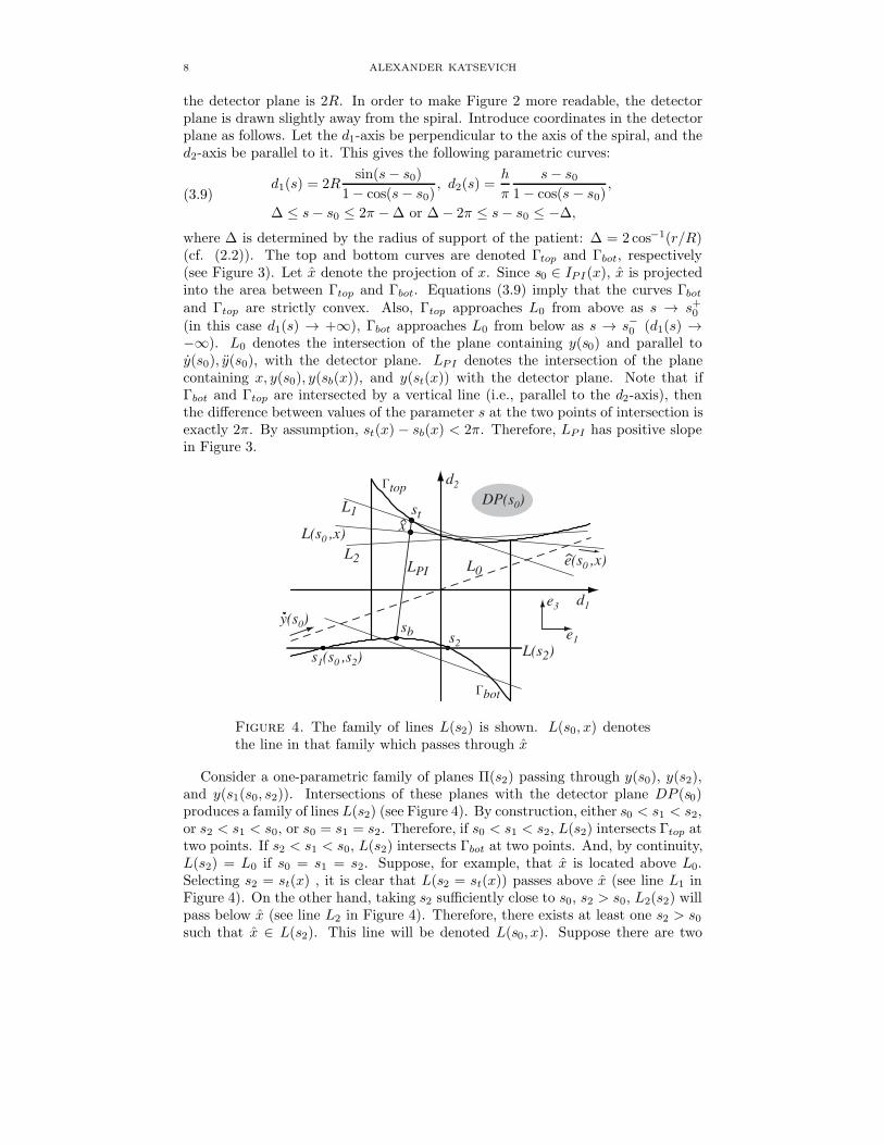
the detector plane is 2R. In order to make Figure 2 more readable, the detectorplane is drawn slightly away from the spiral. Introduce coordinates in the detectorplane as follows. Let the d1-axis be perpendicular to the axis of the spiral, and thed2-axis be parallel to it. This gives the following parametric curves:
d1(s) = 2Rsin(s − s0)
1 − cos(s − s0), d2(s) =
h
π
s − s01 − cos(s − s0)
,
∆ ≤ s − s0 ≤ 2π − ∆ or ∆ − 2π ≤ s − s0 ≤ −∆,
(3.9)
where ∆ is determined by the radius of support of the patient: ∆ = 2 cos−1(r/R)(cf. (2.2)). The top and bottom curves are denoted Γtop and Γbot, respectively(see Figure 3). Let x denote the projection of x. Since s0 ∈ IPI(x), x is projectedinto the area between Γtop and Γbot. Equations (3.9) imply that the curves Γbotand Γtop are strictly convex. Also, Γtop approaches L0 from above as s → s+0(in this case d1(s) → +∞), Γbot approaches L0 from below as s → s−
0 (d1(s) →−∞). L0 denotes the intersection of the plane containing y(s0) and parallel toy(s0), y(s0), with the detector plane. LPI denotes the intersection of the planecontaining x, y(s0), y(sb(x)), and y(st(x)) with the detector plane. Note that ifΓbot and Γtop are intersected by a vertical line (i.e., parallel to the d2-axis), thenthe difference between values of the parameter s at the two points of intersection isexactly 2π. By assumption, st(x) − sb(x) < 2π. Therefore, LPI has positive slopein Figure 3.
Figure 4. The family of lines L(s2) is shown. L(s0, x) denotesthe line in that family which passes through x
Consider a one-parametric family of planes Π(s2) passing through y(s0), y(s2),and y(s1(s0, s2)). Intersections of these planes with the detector plane DP (s0)produces a family of lines L(s2) (see Figure 4). By construction, either s0 < s1 < s2,or s2 < s1 < s0, or s0 = s1 = s2. Therefore, if s0 < s1 < s2, L(s2) intersects Γtop attwo points. If s2 < s1 < s0, L(s2) intersects Γbot at two points. And, by continuity,L(s2) = L0 if s0 = s1 = s2. Suppose, for example, that x is located above L0.Selecting s2 = st(x) , it is clear that L(s2 = st(x)) passes above x (see line L1 inFigure 4). On the other hand, taking s2 sufficiently close to s0, s2 > s0, L2(s2) willpass below x (see line L2 in Figure 4). Therefore, there exists at least one s2 > s0such that x ∈ L(s2). This line will be denoted L(s0, x). Suppose there are two

IMPROVED EXACT FBP ALGORITHM FOR SPIRAL CT 9
values s2, s′2, 0 < s′
2 < s2 < st(x) such that x ∈ L(s2) and x ∈ L(s′2). Since x is
below Γtop, this implies
0 < s1 < s′1 < s′
2 < s2, s1 := s1(s0, s2), s′1 := s1(s0, s′
2).(3.10)
From (2.6), ∂s1/∂s2 = ψ′(s2 − s0) > 0, that is s2 > s′2 implies s1 > s′
1, and thiscontradicts (3.10). Hence, there exists a unique s2, s0 < s2 < st(x), such thatx ∈ Π(s2). The case when x appears below L0 can be considered similarly. Ifx ∈ L0, then the unique solution is s2 = s0.
To prove that s2 = s2(s0, x) depends smoothly on s0 we first consider the casewhen s0 is such that s2(s0, x) and s0 are close. According to the preceding discussionthis happens when s0 → s(x), where s(x) ∈ IPI(x) is the unique value such thatthe plane through y(s(x)) and parallel to y(s(x)), y(s(x)) contains x. It is easilyseen that such s(x) exists and is unique. To simplify the notations, we can assumewithout loss of generality that s(x) = 0. Thus,
x = y(0) + ay(0) + by(0), b > 0.(3.11)
The condition b > 0 follows from x ∈ U . Taking into account terms of the firstorder of smallness and using (2.7), we find analogously to (2.10):
u(s0, s2) =[y(s0) × y(s0)] + [y(s0) × ...
y (s0)] s2−s02 + O((s2 − s0)2)∣∣[y(s0) × y(s0)] + [y(s0) ×
...y (s0)] s2−s0
2 + O((s2 − s0)2)∣∣ , s2 → s0.
(3.12)
Substituting (3.11) and (3.12) into (2.12), implicitly differentiating the resultingequation with respect to s0, and then setting s0 = 0 gives
{b y(0) · (y(0) × ...y (0))}
[1 +
(∂s2/∂s0) − 12
]= 0.(3.13)
Since the expression in braces is not zero, we find
∂s2(s0, x)∂s0
∣∣∣∣s0=s(x)
= −1.(3.14)
Suppose now s0 ∈ (sb(x), st(x)), s0 �= s(x). Instead of solving (2.12) for s2, wecan find the appropriate line L(s2) in Figure 4 which contains x. Let (x1(s0), x2(s0))be the coordinates of x on the detector plane DP (s0). Obviously, these coordinatesdepend smoothly on s0. Consider, for example, the case when x appears above L0.Then s0 < s1 < s2. The equation for s2 is
x2(s0) − d2(s2 − s0)x2(s0) − d2(s1 − s0)
=x1(s0) − d1(s2 − s0)x1(s0) − d1(s1 − s0)
.(3.15)
To simplify the notations, after all differentiations have been carried out the depen-dence of x1,2 on s0 will be dropped and it will be assumed without loss of generalitythat s0 = 0. Multiplying (3.15) out, taking into account s1 − s0 = ψ(s2 − s0), anddifferentiating with respect to s0, we obtain an equation in which ∂s2/∂s0 is mul-tiplied by:
κ :=d′1(s2)(x2 − d2(s1)) + d′
2(s1)ψ′(s2)(x1 − d1(s2))
−d′2(s2)(x1 − d1(s1)) − d′
1(s1)ψ′(s2)(x2 − d2(s2)).
(3.16)
10 ALEXANDER KATSEVICH
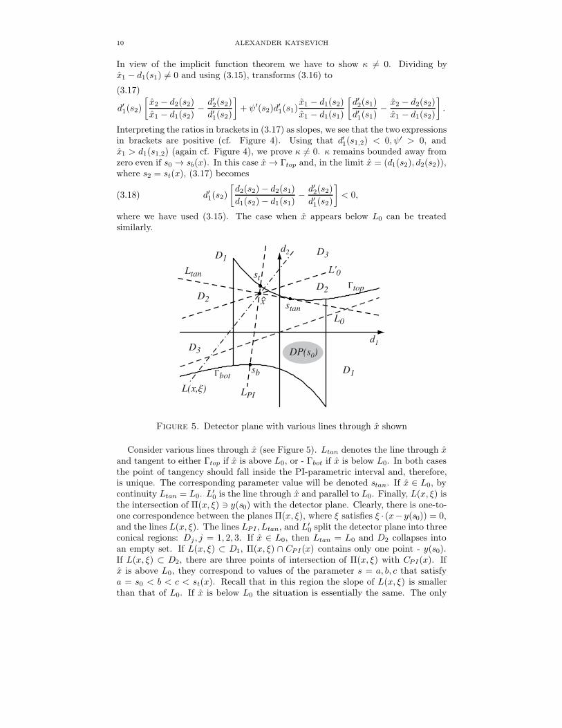
In view of the implicit function theorem we have to show κ �= 0. Dividing byx1 − d1(s1) �= 0 and using (3.15), transforms (3.16) to
d′1(s2)
[x2 − d2(s2)x1 − d1(s2)
− d′2(s2)
d′1(s2)
]+ ψ′(s2)d′
1(s1)x1 − d1(s2)x1 − d1(s1)
[d′2(s1)
d′1(s1)
− x2 − d2(s2)x1 − d1(s2)
].
(3.17)
Interpreting the ratios in brackets in (3.17) as slopes, we see that the two expressionsin brackets are positive (cf. Figure 4). Using that d′
1(s1,2) < 0, ψ′ > 0, andx1 > d1(s1,2) (again cf. Figure 4), we prove κ �= 0. κ remains bounded away fromzero even if s0 → sb(x). In this case x → Γtop and, in the limit x = (d1(s2), d2(s2)),where s2 = st(x), (3.17) becomes
d′1(s2)
[d2(s2) − d2(s1)d1(s2) − d1(s1)
− d′2(s2)
d′1(s2)
]< 0,(3.18)
where we have used (3.15). The case when x appears below L0 can be treatedsimilarly.
Figure 5. Detector plane with various lines through x shown
Consider various lines through x (see Figure 5). Ltan denotes the line through xand tangent to either Γtop if x is above L0, or - Γbot if x is below L0. In both casesthe point of tangency should fall inside the PI-parametric interval and, therefore,is unique. The corresponding parameter value will be denoted stan. If x ∈ L0, bycontinuity Ltan = L0. L′
0 is the line through x and parallel to L0. Finally, L(x, ξ) isthe intersection of Π(x, ξ) � y(s0) with the detector plane. Clearly, there is one-to-one correspondence between the planes Π(x, ξ), where ξ satisfies ξ · (x− y(s0)) = 0,and the lines L(x, ξ). The lines LPI , Ltan, and L′
0 split the detector plane into threeconical regions: Dj , j = 1, 2, 3. If x ∈ L0, then Ltan = L0 and D2 collapses intoan empty set. If L(x, ξ) ⊂ D1, Π(x, ξ) ∩ CPI(x) contains only one point - y(s0).If L(x, ξ) ⊂ D2, there are three points of intersection of Π(x, ξ) with CPI(x). Ifx is above L0, they correspond to values of the parameter s = a, b, c that satisfya = s0 < b < c < st(x). Recall that in this region the slope of L(x, ξ) is smallerthan that of L0. If x is below L0 the situation is essentially the same. The only
IMPROVED EXACT FBP ALGORITHM FOR SPIRAL CT 11
difference is that L(x, ξ) ⊂ D2 implies that parameter values at the three points ofintersection of Π(x, ξ) with CPI(x) satisfy sb < a < b < c = s0. If L(x, ξ) ⊂ D3(an example of such a line is shown in Figure 5), then again there are three pointsof intersection of Π(x, ξ) with CPI(x), and sb(x) < a < b = s0 < c < st(x). Thisargument shows that if ξ ∈ Ξ1 (i.e. when CPI(x) ∩ Π(x, ξ) consists of one point),then L(x, ξ) ⊂ D1. If ξ ∈ Ξ3, then CPI(x) ∩ Π(x, ξ) consists of precisely threepoints and L(x, ξ) ⊂ D2 or D3.
In order to compute the value of the sum in (3.8) we need a simplifying argument.Let ξ be a nonzero vector in the detector plane DP (s0) perpendicular to L(x, ξ)and pointing into the same half-space as ξ, that is ξ · ξ > 0. Fix any nonzerovector e ∈ R
3 perpendicular to β(s0, x), and let L be the line in the intersection ofΠ(x, β(s0, x) × e) with the detector plane. Analogously, e denotes a vector in thedetector plane parallel to L and with the property e · e > 0. We claim that
sgn(ξ · e) = sgn(ξ · e).(3.19)
Indeed, let d0 be the unit vector perpendicular to the detector plane and pointingfrom the source position y(s0) towards the detector (e.g., d0 = y(s0)/|y(s0)|). Thisimplies β(s0, x) · d0 > 0. It is easy to check that
ξ = d0 × (ξ × d0), e = d0 × (e × β(s0, x)).(3.20)
Therefore,
e · ξ = (ξ × d0) · (e × β(s0, x)) = (β(s0, x) · d0)(e · ξ),(3.21)
and (3.19) follows. In (3.21) we have used that β(s0, x) · ξ = 0. Similarly,
ξ · y(s0) = ξ · y(s0)(3.22)
because d0 · y(s0) = 0. Combining (3.19) and (3.22) gives
sgn(ξ · y(s0)) sgn(ξ · e(s0, x)) = sgn(ξ · y(s0)) sgn(ξ · e(s0, x)).(3.23)
For convenience, vectors y(s0) and e(s0, x) are shown in Figure 4.Let us discuss how y(s0) and e(s0, x) should be drawn in Figure 4. By construc-
tion, y(s0) is parallel to the detector plane, that is d0 · y(s0) = 0. Therefore, weshould draw y(s0) parallel to L0 and pointing upward (i.e., y(s0) · e3 > 0). Let e1be the unit vector in the direction of the d1-axis. Then e1 = d0 × e3 (see Figures 2and 4) and
e(s0, x) · e1 ={d0 × [e(s0, x) × β(s0, x)]
}· {d0 × e3} = e3 · [e(s0, x) × β(s0, x)]
= e3 · [(β(s0, x) × u(s0, x)) × β(s0, x)]
= [(β(s0, x) × u(s0, x)] · [β(s0, x) × e3] = u(s0, x) · e3 > 0,
(3.24)
where we have used that e3 · d0 = 0, β(s0, x) · u(s0, x) = 0 (by construction), and(2.11). Therefore, e(s0, x) should point to the right as shown in Figure 4. Notethat if x ∈ L0, then L(s0, x) = L0, e(s0, x) and y(s0) are parallel and point in thesame direction.
To compute B(x, ξ) we have to consider several cases.I. ξ ∈ Ξ1(x). Since in this case Π(x, ξ) ∩ CPI(x) consists of only one point, say
y(s0), L(x, ξ) ⊂ D1 and sgn(ξ · e(s0, x)) = sgn(ξ · y(s0)). Hence, from (3.8) and
12 ALEXANDER KATSEVICH
(3.23):
B(x, ξ) = sgn(ξ · y(s0)) sgn(ξ · e(s0, x)) = 1, ξ ∈ Ξ1(x).(3.25)
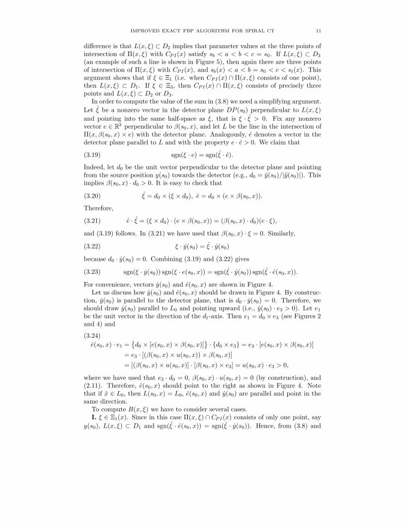
Figure 6. Top half of the detector plane projected from y(a)
II. ξ ∈ Ξ3(x) \ Ξψ(x). In this case there are three points in Π(x, ξ) ∩ CPI(x)corresponding to sb(x) < a < b < c < st(x).
II.1. Consider the detector plane DP (a), where a is the smallest value of theparameter among the three points. Since y(a) is the lowest point of intersectionand there are two more points in Π(x, ξ) ∩ CPI(x), the line L(x, ξ) intersects thepart of Γtop corresponding to a < s < st(x) at two points (see Figure 6).
II.1.a. If c < s2(a, x), then L(x, ξ) passes between L(a, x) and Ltan. This caseis illustrated by Figure 6. Consequently,
sgn(ξ · y(a)) = sgn(ξ · e(a, x)) and sgn(ξ · y(a)) sgn(ξ · e(a, x)) = 1.(3.26)
II.1.b. If c > s2(a, x), then L(x, ξ) passes between L(a, x) and L′0. Conse-
quently,
sgn(ξ · y(a)) = −sgn(ξ · e(a, x)) and sgn(ξ · y(a)) sgn(ξ · e(a, x)) = −1.(3.27)
The case c = s2(a, x) need not be considered because this leads to
{y(s0), y(s2), y(s1(s0, s2))} ∈ Π(x, ξ),(3.28)
which contradicts the assumption ξ �∈ Ξψ(x).II.2. Consider the detector plane DP (b). Since y(b) is the middle point of
intersection, L(x, ξ) passes through D3 because it has to intersect both Γtop andΓbot at s = c, b < c < st(x) and s = a, sb(x) < a < b, respectively. Therefore,
sgn(ξ · y(b)) = sgn(ξ · e(b, x)) and sgn(ξ · y(b)) sgn(ξ · e(b, x)) = 1.(3.29)
II.3. Consider the detector plane DP (c). Since y(c) is the highest point ofintersection and there are two more points in Π(x, ξ) ∩ CPI(x), L(x, ξ) intersectsthe part of Γbot corresponding to sb(x) < s < c at two points.
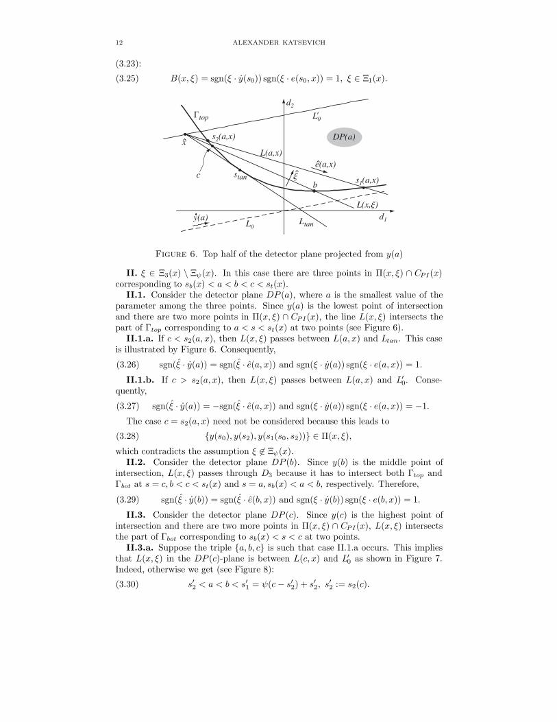
II.3.a. Suppose the triple {a, b, c} is such that case II.1.a occurs. This impliesthat L(x, ξ) in the DP (c)-plane is between L(c, x) and L′
0 as shown in Figure 7.Indeed, otherwise we get (see Figure 8):
s′2 < a < b < s′
1 = ψ(c − s′2) + s′
2, s′2 := s2(c).(3.30)
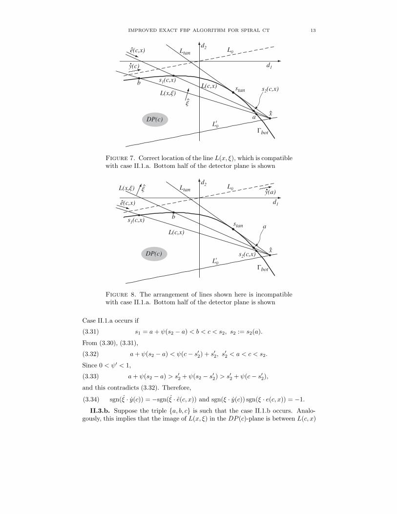
IMPROVED EXACT FBP ALGORITHM FOR SPIRAL CT 13
Figure 7. Correct location of the line L(x, ξ), which is compatiblewith case II.1.a. Bottom half of the detector plane is shown
Figure 8. The arrangement of lines shown here is incompatiblewith case II.1.a. Bottom half of the detector plane is shown
Case II.1.a occurs if
s1 = a + ψ(s2 − a) < b < c < s2, s2 := s2(a).(3.31)
From (3.30), (3.31),
a + ψ(s2 − a) < ψ(c − s′2) + s′
2, s′2 < a < c < s2.(3.32)
Since 0 < ψ′ < 1,
a + ψ(s2 − a) > s′2 + ψ(s2 − s′
2) > s′2 + ψ(c − s′
2),(3.33)
and this contradicts (3.32). Therefore,
sgn(ξ · y(c)) = −sgn(ξ · e(c, x)) and sgn(ξ · y(c)) sgn(ξ · e(c, x)) = −1.(3.34)
II.3.b. Suppose the triple {a, b, c} is such that the case II.1.b occurs. Analo-gously, this implies that the image of L(x, ξ) in the DP (c)-plane is between L(c, x)

14 ALEXANDER KATSEVICH
and Ltan and
sgn(ξ · y(c)) = sgn(ξ · e(c, x)) and sgn(ξ · y(c)) sgn(ξ · e(c, x)) = 1.(3.35)
Let us now summarize. If ξ ∈ Ξ1(x), B(x, ξ) = 1 from (3.25). If ξ ∈ Ξ3(x) \Ξψ(x), there are three points of intersection: sb(x) < a < b < c < st(x). Contri-bution of the middle point y(b) to the sum in (3.8) equals one, and contributionsof the points y(a), y(c) cancel each other (see (3.26) and (3.34), (3.27) and (3.35)).Since the sets Crit(x) and Ξψ(x) have measure zero, the proof is finished.
4. Practical implementation and numerical experiments
In this section we discuss efficient implementations of inversion formulas (2.13)and (2.14). Consider (2.13) first. It is clear from (2.12) that s2(s, x) actuallydepends only on s and β(s, x). Therefore, we can write
u(s, β) := u(s, s2(s, β)), e(s, β) := β × u(s, β), β ∈ S2,
Ψ(s, β) :=∫ 2π
0
∂
∂qDf (y(q), cos γβ + sin γe(s, β))
∣∣∣∣q=s
1sin γ
dγ,
f(x) := − 12π2
∫IP I(x)
1|x − y(s)|Ψ(s, β(s, x))ds.
(4.1)
Fix s2 ∈ [s − 2π + ∆, s + 2π − ∆], s2 �= s, and let Π(s2) denote the plane throughy(s), y(s2), and y(s1(s, s2)). If s2 = s, Π(s2) is determined by continuity andcoincides with the plane through y(s) and parallel to y(s), y(s). The family of linesL(s2) obtained by intersecting Π(s2) with the detector plane is shown in Figure 4.By construction, given any x ∈ U with β(s, x) parallel to Π(s2), s2 used here isprecisely the same as s2 found by solving (2.12). Since e(s, β) · β = 0, |e(s, β)| = 1,we can write (with abuse of notation):
β = (cos θ, sin θ), e(s, β) = (− sin θ, cos θ), β, e(s, β) ∈ Π(s2).(4.2)
Therefore,
Ψ(s, β) =∫ 2π
0
∂
∂qDf(y(q), (cos(θ + γ), sin(θ + γ)))
∣∣∣∣q=s
1sin γ
dγ, β ∈ Π(s2).(4.3)
Equation (4.3) is of convolution type and one application of Fast Fourier Transform(FFT) gives values of Ψ(s, β) for all β ∈ Π(s2) at once.
Equations (4.1) and (4.3) imply that the resulting algorithm is of the filtered-backprojection type. First, one computes shift-invariant filtering of a derivative ofcone beam projections using (4.3) for all s2 ∈ [s−2π+∆, s+2π−∆] (cf. Figure 4).The second step is backprojection according to (4.1). Since ∂/∂q in (4.1) and (4.3)is a local operation, each cone beam projection is stored in memory as soon as ithas been acquired for a short period of time for computing this derivative at a fewnearby points and is never used later.
Comparing (2.13) and (2.14) we see that (2.14) admits absolutely analogousfiltered-backprojection implementation. Moreover, since no derivative with respectto the parameter along the spiral is present, there is never a need to keep morethan one cone beam projection in computer memory at a time.
Consider now the requirements on the detector array imposed by the algorithm.Clearly, they depend on the function ψ in (2.6). In the experiments described belowψ(t) = t/2 and s1(s0, s2) is given by (2.8). From the discussion preceding (4.2) we

IMPROVED EXACT FBP ALGORITHM FOR SPIRAL CT 15
Figure 9. Dashed segments are segments of lines L(s2) locatedbetween Γl and Γr
conclude that given any line L(s2), s2 ∈ [s−2π+∆, s+2π−∆], its segment locatedbetween Γl and Γr should be inside the detector array. These segments are shownin Figure 9. Thus, the left and right boundaries of the required detector array arestill Γl and Γr, but the new top and bottom boundaries are determined using theenvelopes of the lines L(s2). In Figure 9 these boundaries are denoted Γtop and Γbot.As is seen, the detector array required for the algorithm (its area is denoted Aalg)is not much greater than the theoretically minimum one. The latter is bounded byΓtop and Γbot and its area is denoted Amin. The ratio of the areas Aalg/Amin growsas r/R → 1, but slowly. For example, Aalg/Amin = 1.209, 1.230, and 1.255 whenr/R = 0.5, 0.6, and 0.7, respectively. The case r/R = 0.7 is shown in Figure 9.For comparison note that if r/R = 0.5 the algorithm of [Kat01b, Kat01a] requiresa detector array with area 1.93Amin.
Consider L(s2) corresponding to the largest possible value s2 = s + 2π − ∆ (cf.Figure 3). Since s1 = (s + s2)/2 = s + π − ∆/2 < s + π, this line intersects Γtop tothe right of the d2-axis and, therefore, intersects Γr above the point correspondingto s2 = s − 2π + ∆. Hence, the entire segment of this line located between Γl andΓr is inside the detector array and there is no restriction on how big the set Ucan be inside the spiral as long as r/R < 1. This is in contrast with the inversionalgorithm proposed in [Kat01b] (see also [Kat01a]). In the earlier algorithm onehas to know the cone beam data along all lines tangent to Γtop and Γbot at pointsbetween Γl and Γr. Therefore, if r/R is close to one (∆ is close to zero), the linetangent to Γtop at stan = s + 2π − ∆ intersects Γr below the point correspondingto s − 2π + ∆, thereby increasing significantly the required detector array.
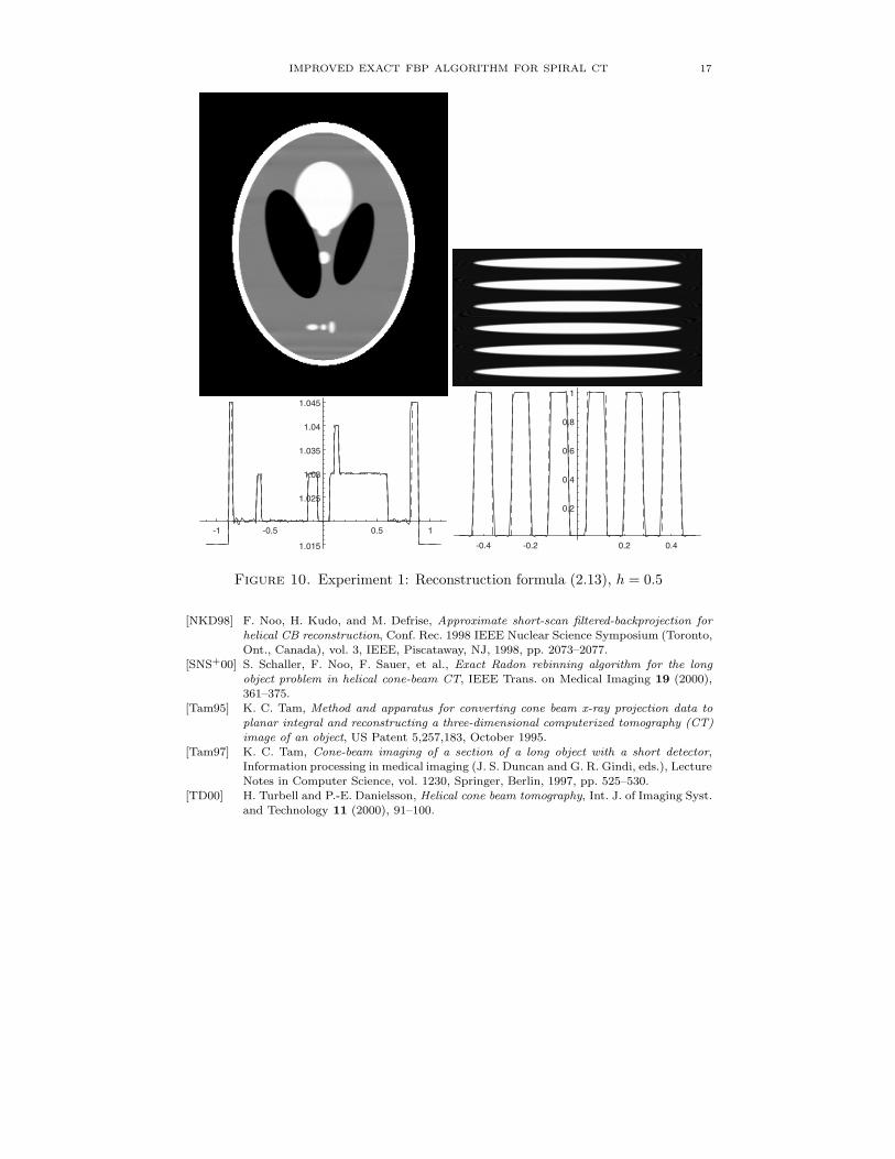
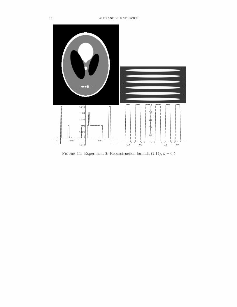
Consider now three numerical experiments. Parameters of the data collectionprotocols are given in Table 1. Reconstructions in Experiment 1 are done using(2.13), and reconstructions in Experiments 2 and 3 are done using (2.14). Theaxial span of the detector array in Experiment 2 is slightly bigger than that inExperiment 1 (despite h being equal in both cases) because to use (2.14) we need alittle extra space for computing derivatives of the data with respect to the angularvariables.

16 ALEXANDER KATSEVICH
Experiment number 1 2 3R (radius of the spiral) 3h (pitch of the spiral) 0.5 0.5 1.0
axial span of the detector array 0.70 0.72 1.44transverse span of the detector array 4.26
number of detector rows 50 50 200number of detectors per row 500
number of source positions per one turn of the spiral 1500 1000 1000
Table 1. Parameters of the data collection protocols
Results of Experiments 1, 2, and 3 are shown in Figures 10, 11, and 12, re-spectively. Left panels of these figures show the 3-D low contrast Shepp phantom(see Table 1 in [KMS98]). Top half demonstrates a vertical slice through the re-constructed image at x1 = −0.25, and bottom half - the graphs of exact (dashedline) and computed (solid line) values of f along a vertical line x1 = −0.25, x2 = 0.We used the grey scale window [1.01, 1.03] to make low-contrast features visible.Right panels of these figures show the disk phantom, which consists of six identi-cal flattened ellipsoids (lengths of half-axes: 0.75, 0.75, and 0.04, distance betweencenters of neighboring ellipsoids: 0.16). Again, top half demonstrates a verticalslice through the reconstructed image at x1 = 0, and the bottom half - the graphsof exact (dashed line) and computed (solid line) values of f along a vertical linex1 = 0, x2 = 0.
References
[B+00] H. Bruder et al., Single slice rebinning reconstruction in spiral cone-beam computedtomography, IEEE Transactions on Medical Imaging 19 (2000), 873–887.
[D+97] P. E. Danielsson et al., Towards exact reconstruction for helical cone-beam scanningof long objects. A new detector arrangement and a new completeness condition, Proc.1997 Meeting on Fully 3D Image Reconstruction in Radiology and Nuclear Medicine(Pittsburgh) (D. W. Townsend and P. E. Kinahan, eds.), 1997, pp. 141–144.
[DNK00] M. Defrise, F. Noo, and H. Kudo, A solution to the long-object problem in helicalcone-beam tomography, Physics in Medicine and Biology 45 (2000), 623–643.
[Kat01a] A. Katsevich, An inversion algorithm for Spiral CT, Proceedings of the 2001 Interna-tional Conference on Sampling Theory and Applications, May 13-17, 2001, Universityof Central Florida (A. I. Zayed, ed.), 2001, pp. 261–265.
[Kat01b] A. Katsevich, Theoretically exact FBP-type inversion algorithm for Spiral CT, (sub-mitted).
[Kat02] A. Katsevich, Microlocal analysis of an FBP algorithm for truncated spiral cone beamdata, Journal of Fourier Analysis and Applications (2002), (to appear).
[KMS98] H. Kudo, N. Miyagi, and T. Saito, A new approach to exact cone-beam reconstructionwithout Radon transform, 1998 IEEE Nuclear Science Symposium Conference Record,IEEE, 1998, pp. 1636–1643.
[KND98] H. Kudo, F. Noo, and M. Defrise, Cone-beam filtered-backprojection algorithm for trun-cated helical data, Phys. Med. Biol. 43 (1998), 2885–2909.
[KS97] H. Kudo and T. Saito, An extended cone-beam reconstruction using Radon transform,1996 IEEE Med. Imag. Conf. Record, IEEE, 1997, pp. 1693–1697.
[KSK00] M. Kachelriess, S. Schaller, and W. A. Kalender, Advanced single-slice rebinning incone-beam spiral CT, Medical Physics 27 (2000), 754–772.
[Lan93] S. Lang, Real and functional analysis, 3rd ed., Springer-Verlag, New York, 1993.
IMPROVED EXACT FBP ALGORITHM FOR SPIRAL CT 17
Figure 10. Experiment 1: Reconstruction formula (2.13), h = 0.5
[NKD98] F. Noo, H. Kudo, and M. Defrise, Approximate short-scan filtered-backprojection forhelical CB reconstruction, Conf. Rec. 1998 IEEE Nuclear Science Symposium (Toronto,Ont., Canada), vol. 3, IEEE, Piscataway, NJ, 1998, pp. 2073–2077.
[SNS+00] S. Schaller, F. Noo, F. Sauer, et al., Exact Radon rebinning algorithm for the longobject problem in helical cone-beam CT, IEEE Trans. on Medical Imaging 19 (2000),361–375.
[Tam95] K. C. Tam, Method and apparatus for converting cone beam x-ray projection data toplanar integral and reconstructing a three-dimensional computerized tomography (CT)image of an object, US Patent 5,257,183, October 1995.
[Tam97] K. C. Tam, Cone-beam imaging of a section of a long object with a short detector,Information processing in medical imaging (J. S. Duncan and G. R. Gindi, eds.), LectureNotes in Computer Science, vol. 1230, Springer, Berlin, 1997, pp. 525–530.
[TD00] H. Turbell and P.-E. Danielsson, Helical cone beam tomography, Int. J. of Imaging Syst.and Technology 11 (2000), 91–100.
18 ALEXANDER KATSEVICH
Figure 11. Experiment 2: Reconstruction formula (2.14), h = 0.5

IMPROVED EXACT FBP ALGORITHM FOR SPIRAL CT 19
Figure 12. Experiment 3: Reconstruction formula (2.14), h = 1.0