Aachen Institute for Advanced Study in Computational Engineering Science

Preprint: AICES-2012/09-1

03/September/2012

Improved Orthogonality for Dense Hermitian

Eigensolvers Based on the MRRR Algorithm

M. Petschow, E. S. Quintana-Ortì, P. Bientinesi

Financial support from the Deutsche Forschungsgemeinschaft (German Research Foundation) through

grant GSC 111 is gratefully acknowledged.

©M. Petschow, E. S. Quintana-Ortì, P. Bientinesi 2012. All rights reserved

List of AICES technical reports: http://www.aices.rwth-aachen.de/preprints

Improved Orthogonality for Dense Hermitian Eigensolvers

based on the MRRR algorithm

A Mixed Precision Approach

M. Petschow ∗, E. S. Quintana-Ortı †, P. Bientinesi ∗

Abstract

The dense Hermitian eigenproblem is of outstanding importance in numericalcomputations and a number of excellent algorithms for this problem exist. Oneof the fastest method is the MRRR algorithm, which is based on a reduction toreal tridiagonal form. This approach, although fast, does not deliver the sameaccuracy (orthogonality) as competing methods like the Divide-and-Conquer orthe QR algorithm. In this paper, we demonstrate how the use of mixed preci-sions in MRRR-based eigensolvers leads to improved orthogonality. At the sametime, when compared to the classical use of the MRRR algorithm, our approachcomes with no or only limited performance penalty, increases the robustness, andimproves scalability.

1 Introduction

In [36], the authors describe how the use of “higher internal precision and mixedinput/output types and precisions [in libraries] permits [...] to implement some al-gorithms that are simpler, more accurate, and sometimes faster.” In particular, theinternal use of higher precision provides the library developer with extra precision anda wider range of values, which may benefit the accuracy and robustness of numericalroutines. As a major difference to software that uses arbitrary precision (e.g., Math-ematica [58], Sage [51], and the LAPACK [2] adaptation MPACK [42]) to obtain anydesired accuracy – as pointed out in [36] – the use of higher precision should not lower“performance significantly if at all.” Our goal is to use mixed precisions to improve theaccuracy, robustness and scalability of solvers for the Hermitian eigenproblem (HEP)based on the fast method of Multiple Relatively Robust Representations (MRRR orMR3 for short) [18, 20, 21] with little or negligible impact on their execution time.

∗RWTH Aachen, Aachen Institute for Advanced Study in Computational Engineering Science,52062 Aachen, Germany. Electronic address: {petschow,pauldj}@aices.rwth-aachen.de

†Depto. de Ingenierıa y Ciencia de Computadores, Universidad Jaume I, 12071 Castellon, Spain.Electronic address: quintana@icc.uji.es

1

The Hermitian eigenproblem consists of finding scalars λ ∈ R and nonzero vectorsv ∈ C

n such that the equationAv = λv (1)

holds for a given Hermitian matrix A ∈ Cn×n. In this case, λ is called an eigenvalue of

A and v is called a corresponding eigenvector. Together, (λ, v) form an eigenpair. TheSpectral Theorem for Hermitian matrices [43] ensures the existence of n eigenpairs(λi, vi) such that the eigenvectors form a complete orthonormal set; that is for alli, j ∈ {1, 2, . . . , n}

v∗j vi =

{1 if j = i ,0 if j 6= i ,

(2)

where we use v∗ to denote the complex-conjugate-transpose of v. Frequently, only theeigenvalues or a subset of eigenpairs are desired. In this paper, we consider the casewhere eigenvectors are computed as well.

For dense matrices, there exist a number of excellent algorithms, which usuallyproceed in three stages: (1) reduction of A to a real symmetric tridiagonal matrixT = Q∗AQ via a unitary similarity transformation; (2) solution of the symmetrictridiagonal eigenproblem Tz = λz; and (3) back-transformation of the eigenvectorsv = Qz. These solvers commonly differ only in the algorithm that is used for thetridiagonal part. Thus, differences in performance and accuracy are attributed to thetridiagonal eigensolver used in the second stage. A study on the performance andaccuracy of various tridiagonal eigensolvers demonstrates that among the fastest isthe MRRR algorithm [16]. Unfortunately, this approach delivers generally the leastaccurate results. These observations carry over to dense eigensolvers that differ onlyin their tridiagonal stage.

For a solver based on the MRRR algorithm, we present how the use of mixed pre-cisions leads to more accurate results at very little or even no extra costs in termsof performance and memory usage. As a consequence, MRRR becomes not only oneof the fastest methods, but also as accurate or even more accurate than the competi-tion. Furthermore, we give compelling experimental evidence that the mixed precisionapproach improves both robustness and parallel scalability. Before we detail the discus-sion, in Section 1.1 we present that all these goals can be achieved for an eigensolverwith single precision input/output.

1.1 Motivating example

High-performance numerical linear algebra libraries such as LAPACK contain routineswith input/output data in the single and double precision formats (defined by theIEEE-754 standard [1, 31]) as these formats and their arithmetic is widely supportedby both computer languages and hardware. We therefore concentrate on the twocases of single precision and double precision input/output. However, to increase theperformance, accuracy, and robustness of routines, numerical libraries can make use ofother data types internally, that is, invisible to the user. Table 1 shows the relevantfloating point formats and their support on our test machine. For example, when we

2

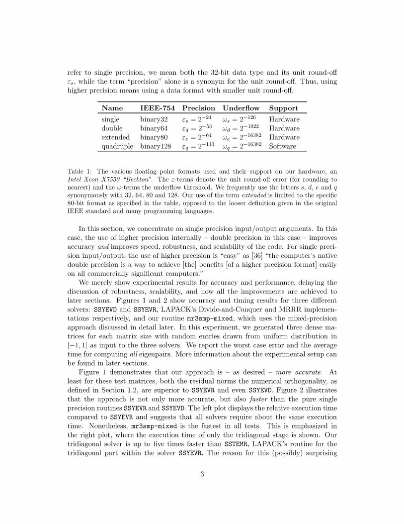
refer to single precision, we mean both the 32-bit data type and its unit round-offεs, while the term “precision” alone is a synonym for the unit round-off. Thus, usinghigher precision means using a data format with smaller unit round-off.

Name IEEE-754 Precision Underflow Support

single binary32 εs = 2−24 ωs = 2−126 Hardwaredouble binary64 εd = 2−53 ωd = 2−1022 Hardwareextended binary80 εe = 2−64 ωe = 2−16382 Hardwarequadruple binary128 εq = 2−113 ωq = 2−16382 Software

Table 1: The various floating point formats used and their support on our hardware, anIntel Xeon X7550 “Beckton”. The ε-terms denote the unit round-off error (for rounding tonearest) and the ω-terms the underflow threshold. We frequently use the letters s, d, e and qsynonymously with 32, 64, 80 and 128. Our use of the term extended is limited to the specific80-bit format as specified in the table, opposed to the looser definition given in the originalIEEE standard and many programming languages.

In this section, we concentrate on single precision input/output arguments. In thiscase, the use of higher precision internally – double precision in this case – improvesaccuracy and improves speed, robustness, and scalability of the code. For single preci-sion input/output, the use of higher precision is “easy” as [36] “the computer’s nativedouble precision is a way to achieve [the] benefits [of a higher precision format] easilyon all commercially significant computers.”

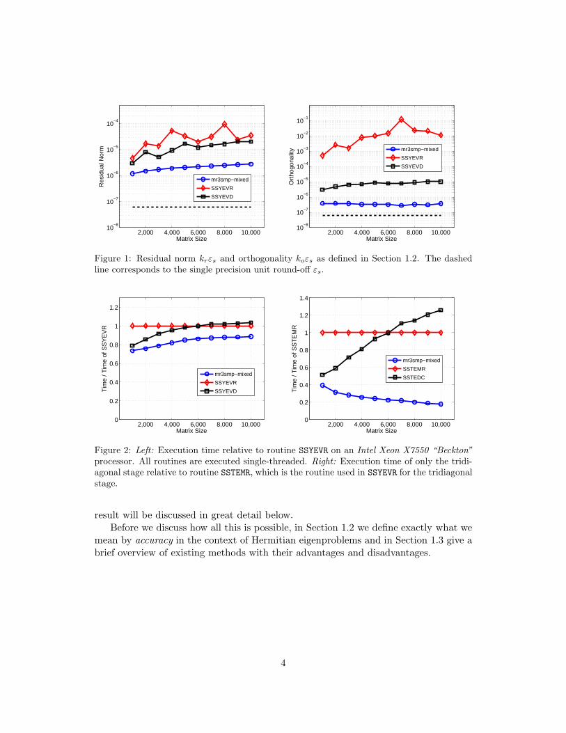
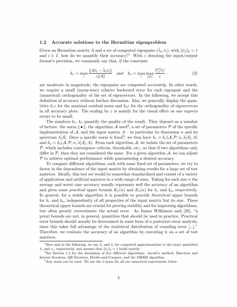
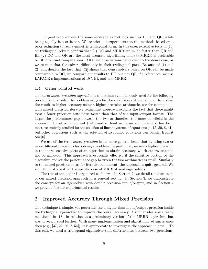
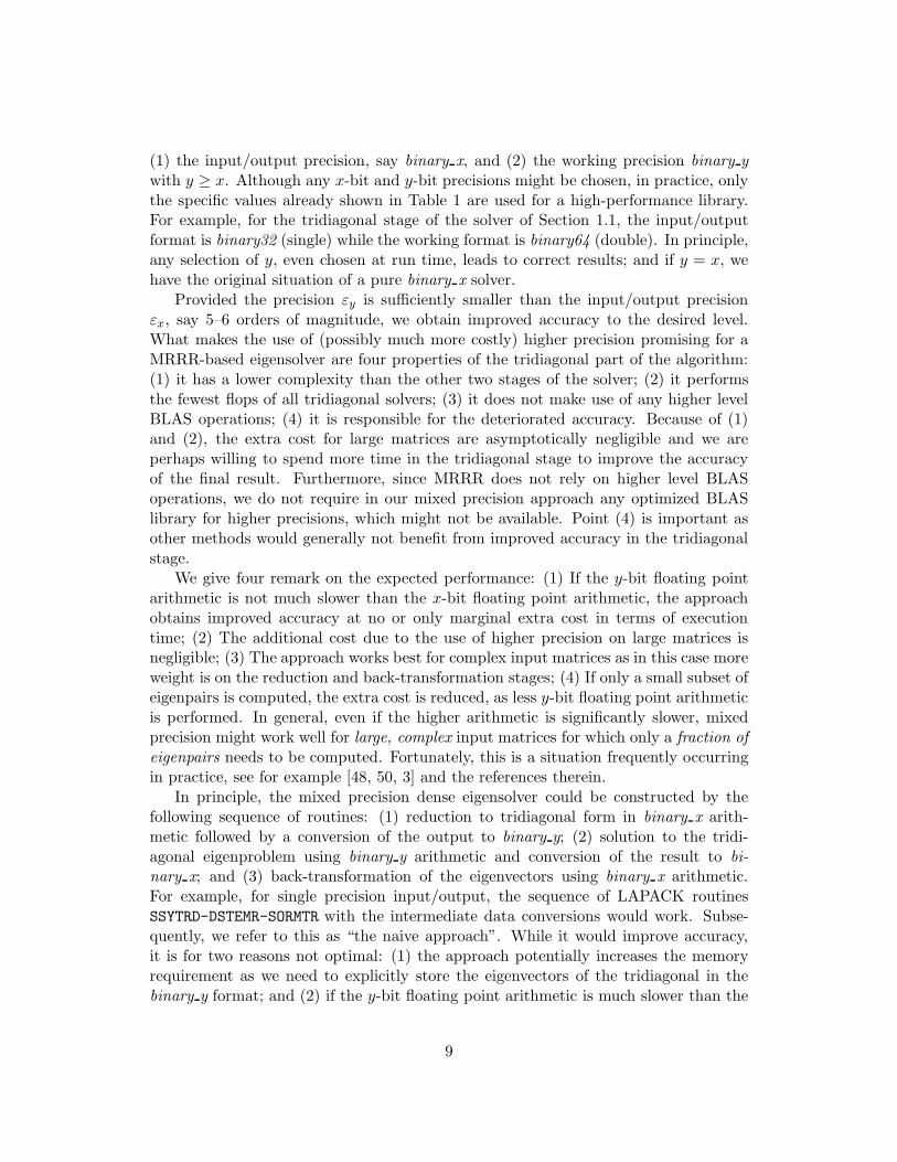
We merely show experimental results for accuracy and performance, delaying thediscussion of robustness, scalability, and how all the improvements are achieved tolater sections. Figures 1 and 2 show accuracy and timing results for three differentsolvers: SSYEVD and SSYEVR, LAPACK’s Divide-and-Conquer and MRRR implemen-tations respectively, and our routine mr3smp-mixed, which uses the mixed-precisionapproach discussed in detail later. In this experiment, we generated three dense ma-trices for each matrix size with random entries drawn from uniform distribution in[−1, 1] as input to the three solvers. We report the worst case error and the averagetime for computing all eigenpairs. More information about the experimental setup canbe found in later sections.

Figure 1 demonstrates that our approach is – as desired – more accurate. Atleast for these test matrices, both the residual norms the numerical orthogonality, asdefined in Section 1.2, are superior to SSYEVR and even SSYEVD. Figure 2 illustratesthat the approach is not only more accurate, but also faster than the pure singleprecision routines SSYEVR and SSYEVD. The left plot displays the relative execution timecompared to SSYEVR and suggests that all solvers require about the same executiontime. Nonetheless, mr3smp-mixed is the fastest in all tests. This is emphasized inthe right plot, where the execution time of only the tridiagonal stage is shown. Ourtridiagonal solver is up to five times faster than SSTEMR, LAPACK’s routine for thetridiagonal part within the solver SSYEVR. The reason for this (possibly) surprising

3

2,000 4,000 6,000 8,000 10,00010

−8

10−7

10−6

10−5

10−4

Res

idua

l Nor

m

Matrix Size

mr3smp−mixed

SSYEVR

SSYEVD

2,000 4,000 6,000 8,000 10,00010

−8

10−7

10−6

10−5

10−4

10−3

10−2

10−1

Ort

hogo

nalit

y

Matrix Size

mr3smp−mixed

SSYEVR

SSYEVD

Figure 1: Residual norm krεs and orthogonality koεs as defined in Section 1.2. The dashedline corresponds to the single precision unit round-off εs.

2,000 4,000 6,000 8,000 10,0000

0.2

0.4

0.6

0.8

1

1.2

Tim

e / T

ime

of S

SY

EV

R

Matrix Size

mr3smp−mixed

SSYEVR

SSYEVD

2,000 4,000 6,000 8,000 10,0000

0.2

0.4

0.6

0.8

1

1.2

1.4T

ime

/ Tim

e of

SS

TE

MR

Matrix Size

mr3smp−mixed

SSTEMR

SSTEDC

Figure 2: Left: Execution time relative to routine SSYEVR on an Intel Xeon X7550 “Beckton”processor. All routines are executed single-threaded. Right: Execution time of only the tridi-agonal stage relative to routine SSTEMR, which is the routine used in SSYEVR for the tridiagonalstage.

result will be discussed in great detail below.Before we discuss how all this is possible, in Section 1.2 we define exactly what we

mean by accuracy in the context of Hermitian eigenproblems and in Section 1.3 give abrief overview of existing methods with their advantages and disadvantages.

4

1.2 Accurate solutions to the Hermitian eigenproblem

Given an Hermitian matrix A and a set of computed eigenpairs (λi, vi), with ‖vi‖2 = 1and i ∈ I, how do we quantify their accuracy?1 With ε denoting the input/outputformat’s precision, we commonly say that, if the constants

kr = maxi

‖Avi − λivi‖ε‖A‖ and ko = max

imaxj 6=i

|v∗j vi|ε

, (3)

are moderate in magnitude, the eigenpairs are computed accurately. In other words,we require a small (norm-wise) relative backward error for each eigenpair and the(numerical) orthogonality of the set of eigenvectors. In the following, we accept thisdefinition of accuracy without further discussion. Also, we generally display the quan-tities krε for the maximal residual norm and koε for the orthogonality of eigenvectorsin all accuracy plots. The scaling by ε is mainly for the visual effect as one expectserrors to be small.

The numbers kr, ko quantify the quality of the result. They depend on a numberof factors: the norm ‖ • ‖, the algorithm A used2, a set of parameters P of the specificimplementation of A, and the input matrix A – in particular its dimension n and itsspectrum λ[A]. Once a specific norm is fixed3, we thus have kr = kr(A,P, n, λ[A], A)and ko = ko(A,P, n, λ[A], A). From each algorithm A, we isolate the set of parametersP, which includes convergence criteria, thresholds, etc., so that if two algorithms onlydiffer in P, then they are considered the same. For a given algorithm A, we can adjustP to achieve optimal performance while guaranteeing a desired accuracy.

To compare different algorithms, each with some fixed set of parameters, we try tofactor in the dependence of the input matrix by obtaining results for a large set of testmatrices. Ideally, this test set would be somewhat standardized and consist of a varietyof application and artificial matrices in a wide range of sizes. Taking for each size n theaverage and worst case accuracy usually represents well the accuracy of an algorithmand gives some practical upper bounds Kr(n) and Ko(n) for kr and ko, respectively.In general, for a stable algorithm it is possible to provide theoretical upper boundsfor kr and ko, independently of all properties of the input matrix but its size. Thesetheoretical upper bounds are crucial for proving stability and for improving algorithms,but often greatly overestimate the actual error. As James Wilkinson said [28], “apriori bounds are not, in general, quantities that should be used in practice. Practicalerror bounds should usually be determined in some form of a posteriori error analysis,since this takes full advantage of the statistical distribution of rounding error [...].”Therefore, we evaluate the accuracy of an algorithm by executing it on a set of testmatrices.

1Here and in the following, we use λi and vi for computed approximations to the exact quantitiesλi and vi, respectively, and assume that ‖vi‖2 = 1 holds exactly.

2See Section 1.3 for the discussion of five different algorithms: Jacobi’s method, Bisection andInverse Iteration, QR Iteration, Divide-and-Conquer, and the MRRR algorithm.

3Any norm can be used. We use the 1-norm for all our numerical experiments below.

5

Similar to the accuracy considerations, the average and worst case execution timescan be used to assess the performance of different methods. This approach is forinstance taken in [16] to evaluate the performance and accuracy of LAPACK’s sym-metric tridiagonal eigensolvers. All performance numbers depend highly on the inputmatrices, the architecture, and the implementation of external libraries, such as vendoroptimized BLAS [24], making the evaluation a difficult task. In our experiments, thetest matrix set is not large enough to draw final conclusions, but the tests suggest gen-eral ideas on the behavior of the algorithms. Our experiments are underpinned by theoutcomes in [16], where results of a large set of test matrices on different architecturesare collected.

1.3 Algorithms for the dense Hermitian eigenproblem

For the solution of dense Hermitian eigenproblems, one is in the luxurious situation ofbeing able to choose among different algorithms: Jacobi’s method, Bisection and In-verse Iteration, QR Iteration, the Divide-and-Conquer method, and the already men-tioned method of Multiple Relatively Robust Representations. The library user isrequired to make a selection among the available algorithms, each of them with itsstrengths and weaknesses and without a clear winner in all situations. At this point,we collect some of the advantages and disadvantages of each method as reported invarious studies, e.g. [12, 14, 28, 43]. As already mentioned, we concentrate on thecase where the eigenvectors are desired. With the exception of Jacobi’s method, allmethods are based on the three-stage approach that initially reduces the input matrixto real symmetric tridiagonal form.

• Jacobi’s method (JM) [32], as stated in [14], “has been very popular, since it isimplemented by a very simple program and gives eigenvectors that are orthog-onal to working accuracy.” It has the advantage of finding eigenvalues to highrelative accuracy whenever this is possible [17, 43]. Furthermore, it is naturallysuitable for parallelism [28, 49] and can be fast on strongly diagonally dominantmatrices. On the downside, in terms of performance, it is usually not competitiveto methods that are based on a reduction to real symmetric tridiagonal form [12].Additionally, JM cannot compute a subset of eigenpairs at reduced cost.

• Bisection and Inverse Iteration (BI) [5, 55] has the advantage of being adaptable,that is, the method may be used to compute a subset of eigenpairs at reducedcost. On the other hand, it was shown that the current software can theoreti-cally fail to deliver correct results [19, 12] and, due to the reorthogonalization ofeigenvectors, its performance suffers severely on matrices with tightly clusteredeigenvalues [12]. While BI has been the method of choice for computing a subsetof eigenpairs for many years, the authors of [16] suggest that today MRRR “ispreferable to BI for subset computations.”

• QR Iteration (QR) [27, 35] is the work horse of dense eigencomputations, es-pecially for unsymmetric and generalized eigenproblems [34, 12]. For the Her-

6

mitian problem the method faces the competition of the Divide-and-Conqueralgorithm, which is usually faster and equally accurate. Recent improvementsreduce this performance handicap, making it almost comparable to the fastestmethods available for computing all eigenpairs [52]. Like Jacobi’s Method, thecurrent implementations of QR are very robust. The method has the distinctfeature that in the dense case it requires the least amount of memory since theeigenvectors can overwrite the initial input matrix [52]. If only a moderate subsetof eigenpairs has to be computed, other methods are preferred.

• Divide-and-Conquer (DC) [10, 29] is among the fastest and most accurate meth-ods available [12, 16]. One advantage of the method lies in the inherent paral-lelism of the divide-and-conquer approach [25]; a second advantage is the relianceon the highly optimized matrix-matrix kernel. DCs drawbacks are that it requiresthe largest amount of memory of all methods [16, 48] and that most implemen-tations cannot be used to compute a subset of eigenpairs at reduced cost; for DCand subset computations see [3].

• Multiple Relatively Robust Representations (MRRR) [18, 20, 21] cures BI from theexplicit reorthogonalization of eigenvectors. As a result, the method is capableof computing k eigenpairs of a tridiagonal matrix in O(nk) operations and hastherefore the lowest worst case complexity of all the tridiagonal eigensolvers. Inthe dense case, this means that the cost of the tridiagonal stage is asymptoticallynegligible compared with the O(n3) cost of the reduction to tridiagonal form.MRRR is the method of choice for computing small subsets of eigenpairs, butoften is the fastest method even when all eigenpairs are desired [16, 47, 48, 7]. Inparticular, as stated in [23], “the MRRR algorithm is usually faster than all othermethods on matrices from industrial applications.” Various studies [48, 47, 7, 54]show its excellent scalability in parallel environments. There are mainly twodisadvantages of MRRR: (1) The computation relies on finding so called relativerobust representations, which are special factorizations of shifted versions of theintermediate tridiagonal matrix that must fulfill certain restrictions, and thereexists the danger of failing to find such representations; (2) In general, MRRRdelivers the least accurate results of all the listed methods. In the dense case,the residual norms of all methods are comparable, but the orthogonality of theeigenvectors computed by MRRR is inferior to the other methods.

To summarize, all methods will generally deliver accurate results – i.e., with krand kc in Eq. (3) of moderate size – but the MRRR-based solvers are less accuratethan the others. In particular, the orthogonality of the eigenvectors can be severalorders of magnitudes worse. On the other hand, MRRR is very fast and the method ofchoice when only a small subset of eigenpairs is desired. In this paper, we address theaccuracy disadvantage of MRRR with a pragmatic approach based on mixed precisions.Additionally, this approach decreases the risk posed by the first of MRRR’s drawback;experimental evidence for this claim is given in Section 4.

7

Our goal is to achieve the same accuracy as methods such as DC and QR, whilebeing equally fast or faster. We restrict our experiments to the methods based on aprior reduction to real symmetric tridiagonal form. In this case, extensive tests in [16]on tridiagonal solvers confirm that (1) DC and MRRR are much faster than QR andBI, (2) DC and QR are the most accurate algorithms, and (3) MRRR is preferableto BI for subset computations. All these observations carry over to the dense case, aswe assume that the solvers differ only in their tridiagonal part. Because of (1) and(2) and despite the fact that [52] shows that dense solvers based on QR can be madecomparable to DC, we compare our results to DC but not QR. As references, we useLAPACK’s implementations of DC, BI, and and MRRR.

1.4 Other related work

The term mixed precision algorithm is sometimes synonymously used for the followingprocedure: first solve the problem using a fast low-precision arithmetic, and then refinethe result to higher accuracy using a higher precision arithmetic, see for example [4].This mixed precision iterative refinement approach exploits the fact that there mightexist a lower precision arithmetic faster than that of the input/output format. Thelarger the performance gap between the two arithmetics, the more beneficial is theapproach. Iterative refinement (with and without using mixed precisions) has beenmost extensively studied for the solution of linear systems of equations [4, 15, 30, 8, 41],but other operations such as the solution of Lyapunov equations can benefit from ittoo [6].

We use of the term mixed precision in its more general form; that is, using two ormore different precisions for solving a problem. In particular, we use a higher precisionin the more sensitive parts of an algorithm to obtain accuracy, which otherwise couldnot be achieved. This approach is especially effective if the sensitive portion of thealgorithm and/or the performance gap between the two arithmetics is small. Similarlyto the mixed precision ideas for iterative refinement, the approach is quite general. Wewill demonstrate it on the specific case of MRRR-based eigensolvers.

The rest of the paper is organized as follows: In Section 2, we detail the discussionof our mixed precision approach in a general setting. In Section 3, we demonstratethe concept for an eigensolver with double precision input/output, and in Section 4we provide further experimental results.

2 Improved Accuracy Through Mixed Precision

The technique is simple, yet powerful: use a higher than input/output precision insidethe tridiagonal eigensolver to improve the overall accuracy. A similar idea was alreadymentioned in [18], in relation to a preliminary version of the MRRR algorithm, butwas never pursued further. With many implementation and algorithmic advances sincethen (e.g., [37, 22, 56, 7, 54]), it is appropriate to investigate the approach in detail. Tothis end, we need a tridiagonal eigensolver that differentiates between two precisions:

8

(1) the input/output precision, say binary x, and (2) the working precision binary ywith y ≥ x. Although any x-bit and y-bit precisions might be chosen, in practice, onlythe specific values already shown in Table 1 are used for a high-performance library.For example, for the tridiagonal stage of the solver of Section 1.1, the input/outputformat is binary32 (single) while the working format is binary64 (double). In principle,any selection of y, even chosen at run time, leads to correct results; and if y = x, wehave the original situation of a pure binary x solver.

Provided the precision εy is sufficiently smaller than the input/output precisionεx, say 5–6 orders of magnitude, we obtain improved accuracy to the desired level.What makes the use of (possibly much more costly) higher precision promising for aMRRR-based eigensolver are four properties of the tridiagonal part of the algorithm:(1) it has a lower complexity than the other two stages of the solver; (2) it performsthe fewest flops of all tridiagonal solvers; (3) it does not make use of any higher levelBLAS operations; (4) it is responsible for the deteriorated accuracy. Because of (1)and (2), the extra cost for large matrices are asymptotically negligible and we areperhaps willing to spend more time in the tridiagonal stage to improve the accuracyof the final result. Furthermore, since MRRR does not rely on higher level BLASoperations, we do not require in our mixed precision approach any optimized BLASlibrary for higher precisions, which might not be available. Point (4) is important asother methods would generally not benefit from improved accuracy in the tridiagonalstage.

We give four remark on the expected performance: (1) If the y-bit floating pointarithmetic is not much slower than the x-bit floating point arithmetic, the approachobtains improved accuracy at no or only marginal extra cost in terms of executiontime; (2) The additional cost due to the use of higher precision on large matrices isnegligible; (3) The approach works best for complex input matrices as in this case moreweight is on the reduction and back-transformation stages; (4) If only a small subset ofeigenpairs is computed, the extra cost is reduced, as less y-bit floating point arithmeticis performed. In general, even if the higher arithmetic is significantly slower, mixedprecision might work well for large, complex input matrices for which only a fraction ofeigenpairs needs to be computed. Fortunately, this is a situation frequently occurringin practice, see for example [48, 50, 3] and the references therein.

In principle, the mixed precision dense eigensolver could be constructed by thefollowing sequence of routines: (1) reduction to tridiagonal form in binary x arith-metic followed by a conversion of the output to binary y; (2) solution to the tridi-agonal eigenproblem using binary y arithmetic and conversion of the result to bi-nary x; and (3) back-transformation of the eigenvectors using binary x arithmetic.For example, for single precision input/output, the sequence of LAPACK routinesSSYTRD-DSTEMR-SORMTR with the intermediate data conversions would work. Subse-quently, we refer to this as “the naive approach”. While it would improve accuracy,it is for two reasons not optimal: (1) the approach potentially increases the memoryrequirement as we need to explicitly store the eigenvectors of the tridiagonal in thebinary y format; and (2) if the y-bit floating point arithmetic is much slower than the

9

x-bit floating point arithmetic, the performance suffers severely. The first issue is ad-dressed in Section 2.1, where we discuss how the computation can be organized so thatthe memory requirements do not grow essentially. The second caveat is addressed inSection 3, where we demonstrate that the mixed precision approach becomes feasibleeven if we need to resort to much slower y-bit floating point arithmetic.

2.1 Memory cost

The memory management in the mixed precision tridiagonal solver is affected by thefact that the eigenvector matrix Z ∈ R

n×k in binary x format is used as intermediatework space. Thus if y > x, this part of the work space is not sufficient anymorefor its customary use, which is the following: for every cluster of two or more closeeigenvalues, the method stores up to 2n binary y numbers in columns of Z. This isgenerally not possible if y > x. If we restrict y ≤ 2x, it is still possible store the 2nbinary y numbers whenever the cluster of eigenvalues is of size four or larger. Thus, thecomputation must be carefully reorganized so that clusters containing less than foureigenvalues are processed without storing any data in Z temporarily. Additionally,after computing an eigenvector in binary y, it is converted to binary x, written into Z,and discarded. Since also some of the bookkeeping can be done using binary x, we donot require (substantially) more memory.

At the beginning of the tridiagonal stage, we must also make a copy of the inputmatrix in order to cast it to binary y. Since in the input is tridiagonal, the memoryincrease due to keeping a copy of the input is rather small. As the result, our mixedprecision approach still needs only O(n) floating point numbers extra work space forthe tridiagonal stage, although (most of) the computation is performed in a higherprecision.

3 A Solver for Double Precision Input/Output

By Table 1 in Section 1.1, when dealing with binary64 input/output arguments, wecan use either binary128 (quadruple) or binary80 (extended) in our mixed precisionapproach. Both cases are analyzed in Section 3.1 and 3.2, respectively.

3.1 Quadruple precision

We discuss the use of quadruple precision first, as it closely resembles the single/doubleprecision case. The major difference is that this time the binary y arithmetic is notsupported by hardware and is therefore much slower than binary x. In general, thesituation corresponds to the case where input/output are in the largest IEEE formatsupported by hardware. Thus, when using quadruple precision for the tridiagonalstage, we must identify which of the computation can still be performed in the muchfaster hardware supported double precision and relax the accuracy requirements of thetridiagonal eigensolver to improve its performance. We use the double/quadruple caseas our case study, but the discussion is general, provided the quantities with index d,

10

such as εd, and with index q are respectively replaced with the indices x and y, and thewords ’double’ and ’quadruple’ are respectively replaced by ’binary x’ and ’binary y’.4

While the mixed precision approach for the single/double case works on virtually anyof today’s processors, the applicability of the double/quadruple case depends on theperformance of the quadruple arithmetic, on the matrix size, and on whether the subsetof eigenpairs to be computed is large.

3.1.1 Optimizing the tridiagonal stage for performance

There are two performance optimization approaches for our tridiagonal eigensolver:(1) Given a double precision eigensolver, replace a minimum of the computation to usequadruple and adjust a minimum of the parameters to guarantee a certain accuracy;(2) Given a quadruple precision eigensolver, use as much of double precision compu-tation and loosen as many of the convergence criteria and thresholds as possible whilestill meeting the accuracy requirements.

We took the second approach as it is incremental: we can only apply some of thechanges without breaking the functionality of the mixed precision solver. In the follow-ing, we give a list of optimizations that can be incorporated. A reader that is merelyinterested in the results, can safely skip to Section 3.1.4 at this point. Otherwise, Al-gorithm 1 presents the MRRR algorithm in sufficient detail for our discussion. Sincethe algorithm heavily uses the concept of so called Relatively Robust Representationsof tridiagonals, we give the following definition adapted from [56].

Definition 3.1. A (partial) Relatively Robust Representation (RRR) of the symmetrictridiagonal T ∈ R

n×n is a set {x1, . . . , xm} of m ≤ 2n − 1 scalars and a mapping f :Rm → R

2n−1 that define the entries of T in such a way that small relative perturbationsxi = xi(1 + ξi), with |ξi| ≤ ξ ≪ 1, will only cause relative changes in (some of) theeigenvalues and eigenvectors of f(x1, . . . , xm) proportional to ξ. In particular, if Mis an RRR for eigenvalue λ, we have |λ − λ| = O(nξ|λ|), where λ is the perturbed 5

eigenvalue of M .

For example, the non-trivial entries of bidiagonal factorizations LDL∗ = T −σI forsome shift σ ∈ R together with the mapping defined by the factorization often form(partial) RRRs and are used in all implementations we consider in this paper. Thus, ifpreferred by the reader, each occurrence of a representation M might be replaced withLDL∗. For a detailed discussion of the MRRR algorithm and the Relatively RobustRepresentations of tridiagonals in particular, we refer to [18, 20, 21, 56] and [45],respectively.

Algorithm 1 requires the input matrix to be unreduced, i.e., all the off-diagonalentries are non-zero. Because of this requirement and an efficiency benefit, small off-diagonal elements are set to zero in a preprocessing step. We discuss this step first.

4Furthermore, in the general discussion, we might assume εx/εy ≥ 105, to improve the orthogonalityto levels of other eigensolvers.

5Here and in the following, we use the notation O(x) informally as “of the order of x in magnitude”.

11

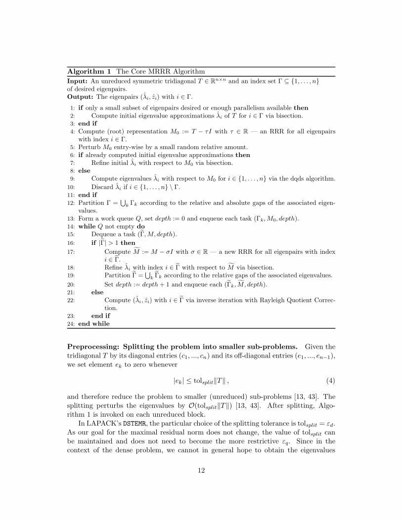
Algorithm 1 The Core MRRR Algorithm

Input: An unreduced symmetric tridiagonal T ∈ Rn×n and an index set Γ ⊆ {1, . . . , n}of desired eigenpairs.Output: The eigenpairs (λi, zi) with i ∈ Γ.

1: if only a small subset of eigenpairs desired or enough parallelism available then

2: Compute initial eigenvalue approximations λi of T for i ∈ Γ via bisection.3: end if

4: Compute (root) representation M0 := T − τI with τ ∈ R — an RRR for all eigenpairswith index i ∈ Γ.

5: Perturb M0 entry-wise by a small random relative amount.6: if already computed initial eigenvalue approximations then7: Refine initial λi with respect to M0 via bisection.8: else

9: Compute eigenvalues λi with respect to M0 for i ∈ {1, . . . , n} via the dqds algorithm.

10: Discard λi if i ∈ {1, . . . , n} \ Γ.11: end if

12: Partition Γ =⋃

k Γk according to the relative and absolute gaps of the associated eigen-values.

13: Form a work queue Q, set depth := 0 and enqueue each task (Γk,M0, depth).14: while Q not empty do

15: Dequeue a task (Γ,M, depth).

16: if |Γ| > 1 then

17: Compute M := M − σI with σ ∈ R — a new RRR for all eigenpairs with indexi ∈ Γ.

18: Refine λi with index i ∈ Γ with respect to M via bisection.19: Partition Γ =

⋃k Γk according to the relative gaps of the associated eigenvalues.

20: Set depth := depth+ 1 and enqueue each (Γk, M , depth).21: else

22: Compute (λi, zi) with i ∈ Γ via inverse iteration with Rayleigh Quotient Correc-tion.

23: end if

24: end while

Preprocessing: Splitting the problem into smaller sub-problems. Given thetridiagonal T by its diagonal entries (c1, ..., cn) and its off-diagonal entries (e1, ..., en−1),we set element ek to zero whenever

|ek| ≤ tolsplit‖T‖ , (4)

and therefore reduce the problem to smaller (unreduced) sub-problems [13, 43]. Thesplitting perturbs the eigenvalues by O(tolsplit‖T‖) [13, 43]. After splitting, Algo-rithm 1 is invoked on each unreduced block.

In LAPACK’s DSTEMR, the particular choice of the splitting tolerance is tolsplit = εd.As our goal for the maximal residual norm does not change, the value of tolsplit canbe maintained and does not need to become the more restrictive εq. Since in thecontext of the dense problem, we cannot in general hope to obtain the eigenvalues

12

to high relative accuracy, we normally employ this absolute splitting criterion. Arelative criterion on the other hand, where ‖T‖ becomes for example

√|ckck+1| and

which might by used for some tridiagonal eigenproblems, requires the tolerance tobecome εq. In both cases, the tolerance for splitting the matrix has no effect on theworst case orthogonality, which depends on the size of the largest sub-problem andtherefore is usually improved by splitting. In the rest of this section, we assume thatthe preprocessing has been done and each sub-problem can be treated independentlyby invoking Algorithm 1. In particular, whenever we refer to matrix T , it is assumedto be unreduced; whenever we reference the matrix size n in the context of parametersettings, it refers to the size of the processed block.

A note on optimizing for performance. Given an MRRR tridiagonal eigensolverfor quadruple precision, we are seeking to relax some of its convergence criteria andthresholds such that we achieve the desired accuracy for the double precision inputand output arguments. Often these parameters can take a wide range of values. Asthe performance not only depends on these parameters in a highly non-trivial fashion,but also on the input matrix, the platform, the performance difference of the dou-ble and quadruple arithmetic, we cannot expect to select “optimal” values withoutsome form of (auto-)tuning these parameters on a specific set of matrices and on aspecific architecture. Nonetheless, we can choose the parameters in a way that givegenerally good performance. Additionally, often the tridiagonal eigensolver is not theperformance bottleneck of the dense eigenproblem, and tuning these parameters is asecondary problem.

To fully understand the parameters and their effect on the accuracy, the readershould be familiar with the basics of the MRRR algorithm in general and the LAPACKimplementation in particular. For a reader that does not have this background, werecommend to read [23] first or skip directly to the results in Section 3.1.4.

3.1.2 Optimizations that do not influence the final accuracy

Some modifications in our tridiagonal eigensolver stem from the fact that we usequadruple precision but require double precision accuracy. The following amendmentsare not perceivable in the output and can therefore equally be used in a tridiagonaleigensolver aiming for quadruple precision accuracy.

Line 2: Convergence criteria for bisection. The bisection procedure relies onthe ability to count the number of eigenvalues smaller than given value µ ∈ R [13].Starting from an interval [λ, λ] known to contain eigenvalue λ, for instance by virtueof the Gerschgorin bounds, bisection reduces the width of the interval by a factortwo at every iteration. The process is converged when the interval satisfies |λ − λ| ≤rtol0 ·max{|λ|, |λ|} or |λ− λ| ≤ atol.

LAPACK’s DSTEMR uses atol = O(ωd) and rtol0 =√εd, i.e., computing the values

to about 8 digits of accuracy (whenever possible). In our solver, we can adjust these

13

parameters. If we desire relative accuracy in this stage, ωd becomes ωq, but we do notneed to select rtol0 =

√εq. Instead, we could for instance retain rtol0 =

√εd. In fact,

there is no obvious functional dependency of rtol0 with the machine precision at all.We therefore changed the parameter to rtol0 = 10−3 for all our experiments. Since theresult will be refined before the eigenvalues are classified, the actual choice of rtol0 isnot crucial, although it influences performance. In principle, we could omit this step(Line 2) entirely.

Line 7 and 18: Convergence criteria for bisection. The intervals from theprevious approximations to the eigenvalues are inflated and used as a starting pointfor limited bisection to refine the eigenvalue with respect to the RRR. The intervalwidth is halved until it satisfies |λ − λ| ≤ max{rtol1 · gap(λ), rtol2 · max{|λ|, |λ|}} or|λ− λ| ≤ atol.

LAPACK’s choice in DSTEMR is rtol1 =√εd and rtol2 = max{5√εd · 10−3, 4εd}.

This reflects the fact that the “eigenvalue needs to be known to high relative accuracyonly at the point when the eigenvector is computed. At intermediate stages, whilethe representation tree is constructed, eigenvalues only need to be accurate enough todistinguish between large and small relative gaps” [53]. In our situation, we do notneed to change rtol1 and rtol2 if also the minimum relative gap, given by the parametergaptol (see below), remains mainly unchanged. For various reasons, we prefer to usesmaller values for gaptol and possibly double precision arithmetic for the bisectioncomputation. Thus, we choose rtol1 = rtol2 = max{5 · gaptol · 10−3, 4εd}.

A side note: “if the proportion of desired eigenpairs is high enough or the fullspectrum has to be computed, then all eigenvalues are computed by the more efficientdqds algorithm and unwanted ones are discarded” [23]. However, bisection might bemore efficient – even if all the eigenvalues are needed – in a parallel environment. Wetherefore need to decide whether the dqds algorithm or bisection is used for the initialeigenvalue computation in Lines 1 to 11, see [47]. The changes in the convergencecriteria and the precision used (see below) for the computations both influence theminimal amount of parallelism necessary for bisection to become faster than dqds.

Line 9: Precision used in the dqds algorithm. If the dqds algorithm is chosen,let Zq = (q1, e1, q2, e2, . . . , qn, en) be the quadruple precision input – as defined forexample in [46] – to a specific implementation of the algorithm and Zd be Zq cast todouble precision. Then the conversion Zq to Zd corresponds to an element-wise relativeperturbation of at most εd. Since Zq is an RRR for all eigenvalues, and by Def. 3.1, theexact eigenvalues λq and λd of respectively Zq and Zd satisfy |λq − λd| = O(nεd|λd|).A double precision implementation of the dqds algorithm such as LAPACK’s DLASQ2produces eigenvalues λd to high relative accuracy, that is |λd−λd| = O(nεd|λd|). Thus,our computed eigenvalues satisfy |λq − λd| ≤ |λq − λd| + |λd − λd| = O(nεd|λd|). Asa final cast of the result to quad precision introduces no additional error, we obtainthe eigenvalues with relative error of O(nεd). This is more than required, provided weprohibit gaptol from being too small, to classify the eigenvalues. In this way, we can

14

perform a (noticeable) portion of the computation in the much faster double precisionarithmetic.

Line 7 and 18: Precision used for bisection. By the same argument, we can usethe much faster double precision computation when refining the eigenvalues. In Lines7 and 18, given representation Mq in quadruple precision. A conversion to double, thatis to Md, corresponds to relative perturbations in the entries of Mq. The refinement of

the eigenvalue λd with respect toMd via bisection in double precision with a conversionto the quadruple yields |λq − λq| = O(tol · |λq|), where the convergence parameter tolis chosen as discussed above.6

Note that in order to avoid under-/overflow in the double precision execution, itmight be necessary that the input matrix T is scaled as in a pure double precision solver.This depends on the specific implementation of the bisection routine, see [13, 38]. Also,the relative convergence criterion cannot be taken smaller than what is achievable bybisection executed double precision.

As the initial eigenvalue approximation and refinement of eigenvalues can makeup for a noticeable portion of the overall computation, the use of double precisionarithmetic for these parts can speed up the mixed precision approach considerably inthose cases where quadruple precision arithmetic is performed rather slow, e.g., whenit is simulated in software.

3.1.3 Optimizations that influence the final accuracy

The following optimizations reflect the fact that we are not aiming for quadruple pre-cision accuracy in the tridiagonal stage. The list is not exhaustive, but concentrates onthe parameters that influence performance the most. Additionally, the freedom in theparameter selection due to the relaxed accuracy requirement may be used to increaserobustness and scalability as well; both aspects are discussed further in Section 4.

Line 5: Random perturbation of the root representation. The elements ofthe representation M0, {x1, ..., xm}, are perturbed by small random relative amountsxi = xi(1+ ξi) with |ξi| ≤ ξ for all 1 ≤ i ≤ m to break up tight clusters. This idea andits importance for robustness is discussed in detail in [22].

DSTEMR uses ξ = 8εd, which is perturbing each entry by a few units in the lastplace. In our situation, we can be more aggressive, using ξ = εd. Thus, about half ofthe digits in each entry of the representation M0 are chosen randomly. This has twomajor effects: (1) it becomes very unlikely to encounter clusters within clusters underthe classification criterion described below and (2) it helps significantly in finding anRRR with a shift close to one end of a cluster.

6At this point, we could use Mq to ensure at the cost of two Sturm counts per eigenvalue that theapproximation as accurate as required. If not, the corresponding interval could be inflated and refinedin quadruple precision. A similar approach could be taken after the double precision dqds algorithmwas used.

15

Line 12 and 19: Minimum relative gap. The unfolding of Algorithm 1 highlydepends on how the sets Γ and Γ are partitioned in Line 12 in Line 19, respectively.The criterion is based on the absolute and relative gap of the eigenvalues. To justifythe choice made, we invoke the following classical theorem that can be found in similarform for example in [43, 12].

Theorem 3.1. Given T (by any representation) and an approximation (λ, z), with‖z‖2 = 1, to the eigenpair (λ, z), let r be the residual T z − λz; then

sin∠(z, z) ≤ ‖r‖2gap(λ)

, (5)

with gap(λ) = minj{|λ− λj | : λj 6= λ}. Proof: See [43, 12, 56, 11].

In order to achieve sin∠(z, z) = O(nε), we must be able to compute residual normswith ‖r‖2 = O(nεgap(λ)). Unfortunately, this is not always possible. In particular, ifgap(λ) ≪ ‖T‖2, we cannot expect convergence of standard inverse iteration [18, 19].One of the features of the MRRR algorithm is the computation of eigenpairs with‖r‖2 = O(nε|λ|) [44, 21]. Thus, provided gap(λ) & |λ|, say gap(λ)/|λ| > gaptol, wecan achieve sin∠(z, z) ≤ O(nε/gaptol). The choice of gaptol is restricted by the loss oforthogonality that we are willing to accept. In practice, the value is often chosen to be10−3, reflecting a compromise between achievable orthogonality and practicality [20].

When our working precision becomes quadruple, the requirement can be relaxed.We have

sin∠(z, z) ≤ O(

nεqgaptol

), (6)

and the value of gaptol can be chosen (at least) as small as εq√n/εd ≈ 10−18

√n.

The particular choice7 of gaptol affects performance in multiple ways: the conver-gence criteria for bisection depend explicitly on it, and in order to use double precisioncomputations of the eigenvalues as discussed above, the value cannot be chosen toosmall. On the other hand, the smaller the value of gaptol the less clustering of eigen-values occurs – resulting in beneficial performance. Taking these considerations intoaccount, we restricted gaptol to the interval [10−12, 10−3] and optimized the value forperformance. For the experimental results shown in later sections, we fixed gaptol to10−10.

Line 12: Minimum absolute gap. A classification of the eigenvalues based ontheir relative gaps alone can lead to bulky clusters, especially for large-scale problems.In order for an eigenvalue λ to be classified as well-separated by the relative criterion,we require

gap(λ) > gaptol · |λ| , (7)

7In the more general case, min{10−3, εy√n/εx} ≤ gaptol ≤ 10−3.

16

i.e., the absolute gap for an eigenvalue large in magnitude must be equally large; eventhough some of the eigenvalues might be well-separated from the others in an absolutesense, they might not be in the relatively sense.

Large clusters can lead to deteriorated performance and impose problems for paral-lel distributed-memory codes such as [48, 54, 7]. The problem and how to overcome itis discussed in detail in [53, 54]. The solution is to supplement the relative classificationcriterion in Line 12 with one that takes also the absolute gap of the eigenvalues intoaccount. Using a small adaption of the criterion in [53, 54], we classify an eigenvalueas well-separated if

gap(λ) >|λn − λ1|n− 1

= avgap , (8)

and additionally split clusters of eigenvalues into smaller clusters whenever the clusterhas a separation from the rest of the spectrum greater than the average gap, avgap.This criterion can be justified by the analog of Theorem 3.1 for invariant subspacesof any dimension, see [43, 56, 11, 14, 53]. In fact, we could relax this condition toα · avgap with α ≪ 1, if we also reduce the convergence criterion for inverse iterationaccordingly and adjust gaptol. For practical matrices, the effect on performance isminor and we used α = 1 in all experiments.

Line 22: Stopping criteria for inverse iteration. The MRRR algorithm usu-ally performs Rayleigh Quotient iteration with twisted factorizations (controlled bybisection), a process described in detail in [23, 56, 53]. An eigenpair is accepted if‖r‖2 ≤ tol1 · gap(λ), or if the ’Rayleigh Quotient Correction’ ≤ tol2 · |λ| and thereforecannot improve the eigenvalue approximation. The convergence criteria are discussedfor example in [53].

DSTEMR uses tol1 = 4εd log n and tol2 = 2εd. While tol2 must becomeO(εq), in mostcases we can stop the inverse iteration process earlier by relaxing the tol1 parameter.We chose tol1 = 4εd and tol2 = 2εq for the experiments.

3.1.4 The effect of the changes to performance and accuracy

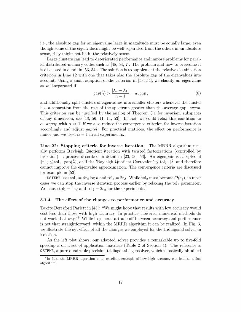
To cite Beresford Parlett in [43]: “We might hope that results with low accuracy wouldcost less than those with high accuracy. In practice, however, numerical methods donot work that way.”8 While in general a trade-off between accuracy and performanceis not that straightforward, within the MRRR algorithm it can be realized. In Fig. 3,we illustrate the net effect of all the changes we employed for the tridiagonal solver inisolation.

As the left plot shows, our adapted solver provides a remarkable up to five-foldspeedup a on a set of application matrices (Table 2 of Section 4). The reference isQSTEMR, a pure quadruple precision tridiagonal eigensolver, which is basically obtained

8In fact, the MRRR algorithm is an excellent example of how high accuracy can lead to a fastalgorithm.

17

by automatically translating LAPACK’s DSTEMR by replacing DOUBLE PRECISION datatypes with REAL*16 (quadruple) data types.

Such performance gains are not a miracle, but stem from our willingness to giveup accuracy up to a certain level. This is depicted by the accuracy of our solutions inFig. 3 (right).9 Note that there is nothing special about the line given by εd; in fact,we can achieve any accuracy that is not better than the quadruple precision result. Inour context however, it makes no sense to further reduce residuals and orthogonalitysince the results will be converted to double precision. At this place, we also wantto point to Fig. 2 again, as now it becomes understandable why our mixed precisionapproach is faster than SSYEVR for single precision input/output.

2,053 4,289 7,923 12,387 16,0230

0.2

0.4

0.6

0.8

1

Tim

e / T

ime

of Q

ST

EM

R

Matrix Size

Quad solver QSTEMR

mr3smp−mixed

2,053 4,289 7,923 12,387 16,02310

−35

10−30

10−25

10−20

10−15

10−10

Res

idua

l Nor

m &

Ort

hogo

nalit

y

Matrix Size

QSTEMR (residual)

QSTEMR (orthogonality)

mr3smp−mixed (residual)

mr3smp−mixed (orthogonality)

Figure 3: Left: Execution time of our adapted tridiagonal solver mr3smp-mixed relative tothe quad precision routine QSTEMR computing all eigenpairs. Left: Corresponding accuracy formr3smp-mixed and QSTEMR. As a reference, we added εd and εq as black dashed lines.

3.1.5 Portability of using quadruple precision

Presently, there are two major drawbacks in using quadruple precision: (1) it is ratherslow and (2) the support through compilers and languages is limited. These draw-backs make it hard to produce portable code that runs at reasonable performanceon different architectures with different compilers. In FORTRAN, it is possible toproduce portable code by using the REAL*16 data type. But, this type might not besupported by all compilers. In a C/C++ environment, the support is entirely compilerdependent. It is for instance supported via the float128 and Quad data types withthe GNU compilers and the Intel compilers, respectively. Alternatively, an externallibrary implementing the software arithmetic might be used for portability. In anycase, if quadruple precision is available, the performance highly depends on the spe-cific implementation. Most likely, the support for quadruple precision will be improved

9In this experiments, we kept all the eigenpairs in quadruple precision in order to compute theirresiduals and the orthogonality in quadruple.

18

in the future.

3.2 Extended precision

Quadruple precision arithmetic is rather slow, as there exist no widespread hardwaresupport at the time of writing. But, many current architectures have hardware supportfor a 80-bit extended floating point format (see Table 1). According to William Ka-han [33] “this format is intended mainly to help programmers enhance the integrity oftheir Single and Double software, and to attenuate degradation by round-off in Doublematrix computations of larger dimensions, and can easily be used in such a way thatsubstituting Quadruple for Extended need never invalidate its use.” Our situation fitsinto this picture.

As the unit round-off εe is only about three orders of magnitude smaller than εd, wecannot expect our orthogonality to be improved by more than this amount. The mainadvantage of the extended format is that compared to double precision its arithmeticcomes without any or only a small loss in speed.10 We therefore expect in all situationsimproved accuracy without any significant loss in performance. This is confirmed inall test we performed: the tridiagonal stage was never slowed down more than bya factor of two, which results in negligible extra cost for the dense eigensolver. Thesituation is slightly different between the double/extended and double/quadruple cases;in contrast to the double/quadruple case, we cannot relax the accuracy requirementsof the tridiagonal eigensolver when using extended precision – all the extra precisionis necessary to improve accuracy. Thus, even if the arithmetic is performed exactly atthe same speed, we cannot expect the mixed precision eigensolver using extended tobe faster than a solver using pure double precision exclusively.

Experimental results suggest that in many cases the MRRR-based eigensolver usingextended precision obtains orthogonality comparable to that of methods such DC orQR. On the other hand, especially for larger matrices, the use of extended precisionpotentially leads to an orthogonality that is inferior to other methods (see Section 4).

3.2.1 Portability of using extended precision

Not all architectures support the 80-bit extended floating point format, so that itsuse is not generally portable. A C/C++ code that uses the long double data type(introduced in ISO C99) for the higher precision in the tridiagonal solver would achievethe desired result on most architectures. However, some compilers might interpret longdouble as either double or rarely even quadruple. In the first case, we do not gain(or lose) anything. In the later case, we gain accuracy but might lose performancedepending on how quadruple is supported. FORTRAN code making use of extendedprecision is likely not to be portable, as not all compilers support the extended precisionformat REAL*10.

10A loss in performance might appear for two reasons: (1) the ability to use vectorized operationsis lost, and (2) the algorithm is memory-bandwidth limited.

19

4 Experimental Results

So far we have not listed the details of the experimental results of the previous sections.At this point, we want to catch up on this. For all LAPACK results, we used version3.3 in conjunction with version 10.2 of Intel MKL BLAS. For the mixed precisionresults, we used the same reduction and back-transformation routines as LAPACK inconjunction with a modified mixed precision version of the parallel solver presentedin [47]. For the extended precision results, we used version 4.7 of the GNU compilers.In all other experiments, we used version 12.1 of Intel’s compiler.11 In all cases, weenabled optimization level -O3. All experiments were performed single-threaded on aIntel Xeon X7550 “Beckton” processor with nominal clock speed of 2 GHz.

In the single/double experiment of Section 1.1, we applied all the adjustmentsdiscussed in Section 3.1, with only one exception: we do not resort to single precisionarithmetic in the dqds algorithm and bisection. In the double/extended experiments,we merely used extended as our higher precision arithmetic; in the double/quadruplecase, we applied all the discussed changes.

Since for single precision input/output the mixed precision approach works verywell, here we concentrate on double precision input/output. In this case, the mixedprecision approach uses either extended or quadruple precision. We refer to thesecases as mr3smp-extended and mr3smp-quad, respectively. The use of quadruple ismore critical as it shows that the approach is applicable in many circumstances, evenwhen the higher precision arithmetic used in the tridiagonal stage is much slower thanarithmetic in the input/output format.

In this section, we confine ourselves to experiments on a small set of applicationmatricesas listed in Table 2, coming from quantum chemistry and structural mechanicsproblems.12 As the performance of the eigensolvers highly depend on the spectra ofthe input matrices, the platform of the experiment, the used BLAS library, and theimplementation of the quadruple arithmetic, we cannot draw final conclusions aboutperformance from these limited test. On the other hand, the orthogonality improve-ments are quite general and are observed also for a much larger test set originatingfrom [39]. We do not report on residuals as the worst case residual norms are generallycomparable for all solvers.

To better display the effects of the use of mixed precisions, the performance resultsare simplified in the following sense: As the routines for the reduction to tridiagonalform and the back-transformation of all solvers are exactly the same, we used for thesestages the minimum execution time of all runs for each solver. In this way, the costof the mixed precision approach becomes more visible and we do not have to resort tostatistical metrics for the timings. We point out that especially for the subset tests,the run time of the tridiagonal stage for larger matrices is often smaller than the

11For all timings, we only compare routines compiled with the same compiler. That is the routinesusing extended are compared to routines compiled with the GNU compilers.

12These matrices are stored in tridiagonal form. In order to create real and complex dense matrices,we generated a random Householder matrix H = I − τvv∗ and applied the similarity transformationHTH to the tridiagonal matrix T .

20

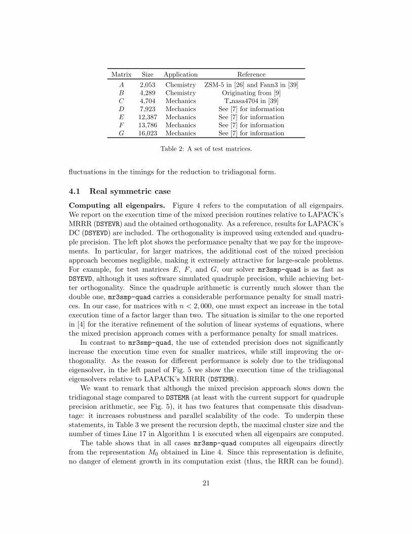
Matrix Size Application Reference

A 2,053 Chemistry ZSM-5 in [26] and Fann3 in [39]B 4,289 Chemistry Originating from [9]C 4,704 Mechanics T nasa4704 in [39]D 7,923 Mechanics See [7] for informationE 12,387 Mechanics See [7] for informationF 13,786 Mechanics See [7] for informationG 16,023 Mechanics See [7] for information

Table 2: A set of test matrices.

fluctuations in the timings for the reduction to tridiagonal form.

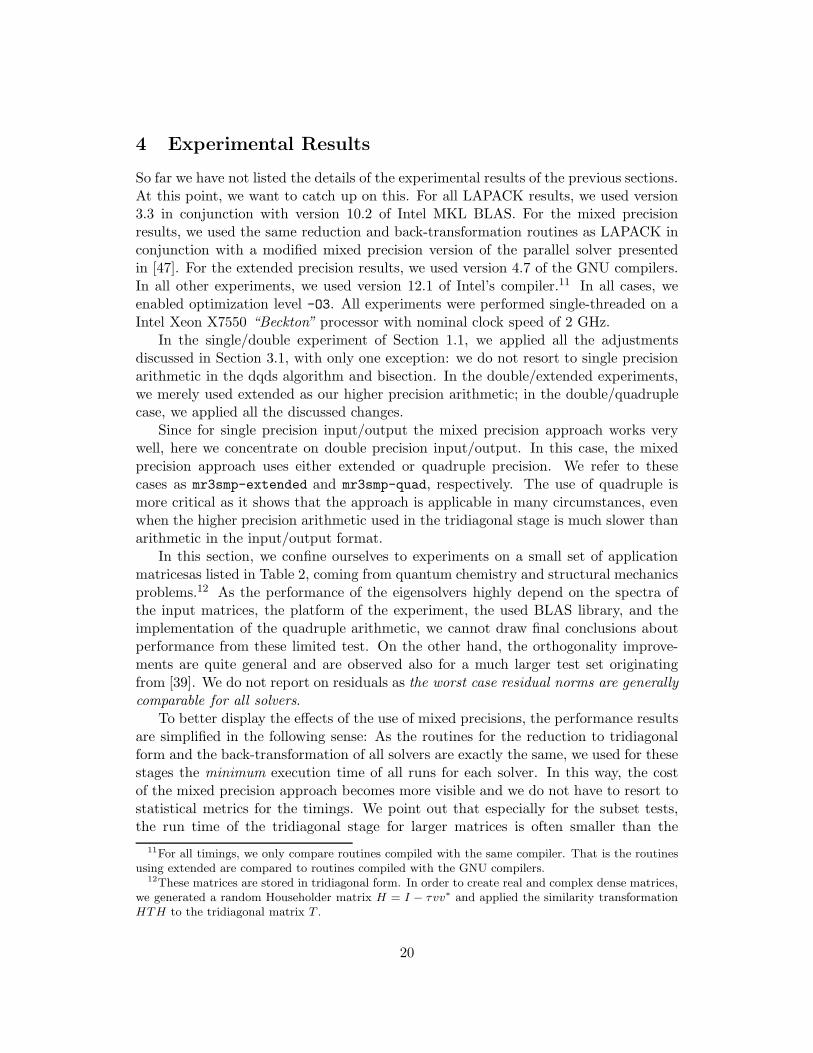
4.1 Real symmetric case

Computing all eigenpairs. Figure 4 refers to the computation of all eigenpairs.We report on the execution time of the mixed precision routines relative to LAPACK’sMRRR (DSYEVR) and the obtained orthogonality. As a reference, results for LAPACK’sDC (DSYEVD) are included. The orthogonality is improved using extended and quadru-ple precision. The left plot shows the performance penalty that we pay for the improve-ments. In particular, for larger matrices, the additional cost of the mixed precisionapproach becomes negligible, making it extremely attractive for large-scale problems.For example, for test matrices E, F , and G, our solver mr3smp-quad is as fast asDSYEVD, although it uses software simulated quadruple precision, while achieving bet-ter orthogonality. Since the quadruple arithmetic is currently much slower than thedouble one, mr3smp-quad carries a considerable performance penalty for small matri-ces. In our case, for matrices with n < 2, 000, one must expect an increase in the totalexecution time of a factor larger than two. The situation is similar to the one reportedin [4] for the iterative refinement of the solution of linear systems of equations, wherethe mixed precision approach comes with a performance penalty for small matrices.

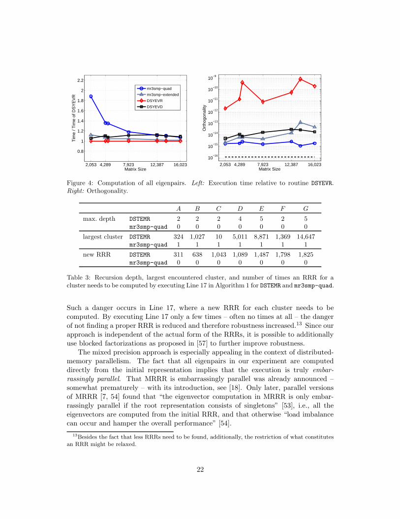
In contrast to mr3smp-quad, the use of extended precision does not significantlyincrease the execution time even for smaller matrices, while still improving the or-thogonality. As the reason for different performance is solely due to the tridiagonaleigensolver, in the left panel of Fig. 5 we show the execution time of the tridiagonaleigensolvers relative to LAPACK’s MRRR (DSTEMR).

We want to remark that although the mixed precision approach slows down thetridiagonal stage compared to DSTEMR (at least with the current support for quadrupleprecision arithmetic, see Fig. 5), it has two features that compensate this disadvan-tage: it increases robustness and parallel scalability of the code. To underpin thesestatements, in Table 3 we present the recursion depth, the maximal cluster size and thenumber of times Line 17 in Algorithm 1 is executed when all eigenpairs are computed.

The table shows that in all cases mr3smp-quad computes all eigenpairs directlyfrom the representation M0 obtained in Line 4. Since this representation is definite,no danger of element growth in its computation exist (thus, the RRR can be found).

21

2,053 4,289 7,923 12,387 16,023

0.8

1

1.2

1.4

1.6

1.8

2

2.2

Tim

e / T

ime

of D

SY

EV

R

Matrix Size

mr3smp−quad

mr3smp−extended

DSYEVR

DSYEVD

2,053 4,289 7,923 12,387 16,023

10−16

10−15

10−14

10−13

10−12

10−11

10−10

10−9

Ort

hogo

nalit

y

Matrix Size

Figure 4: Computation of all eigenpairs. Left: Execution time relative to routine DSYEVR.Right: Orthogonality.

A B C D E F G

max. depth DSTEMR 2 2 2 4 5 2 5mr3smp-quad 0 0 0 0 0 0 0

largest cluster DSTEMR 324 1,027 10 5,011 8,871 1,369 14,647mr3smp-quad 1 1 1 1 1 1 1

new RRR DSTEMR 311 638 1,043 1,089 1,487 1,798 1,825mr3smp-quad 0 0 0 0 0 0 0

Table 3: Recursion depth, largest encountered cluster, and number of times an RRR for acluster needs to be computed by executing Line 17 in Algorithm 1 for DSTEMR and mr3smp-quad.

Such a danger occurs in Line 17, where a new RRR for each cluster needs to becomputed. By executing Line 17 only a few times – often no times at all – the dangerof not finding a proper RRR is reduced and therefore robustness increased.13 Since ourapproach is independent of the actual form of the RRRs, it is possible to additionallyuse blocked factorizations as proposed in [57] to further improve robustness.

The mixed precision approach is especially appealing in the context of distributed-memory parallelism. The fact that all eigenpairs in our experiment are computeddirectly from the initial representation implies that the execution is truly embar-rassingly parallel. That MRRR is embarrassingly parallel was already announced –somewhat prematurely – with its introduction, see [18]. Only later, parallel versionsof MRRR [7, 54] found that “the eigenvector computation in MRRR is only embar-rassingly parallel if the root representation consists of singletons” [53], i.e., all theeigenvectors are computed from the initial RRR, and that otherwise “load imbalancecan occur and hamper the overall performance” [54].

13Besides the fact that less RRRs need to be found, additionally, the restriction of what constitutesan RRR might be relaxed.

22

2,053 4,289 7,923 12,387 16,0230

1

2

3

4

5

6

7T

ime

/ Tim

e of

LA

PA

CK

’s M

RR

R

Matrix Size

mr3smp−quad

mr3smp−extended

LAPACK’s MRRR

LAPACK’s DC

2,053 4,289 7,923 12,387 16,0230

5

10

15

20

25

30

Tim

e / T

ime

of L

AP

AC

K’s

MR

RR

Matrix Size

mr3smp−quad

mr3smp−extended

LAPACK’s MRRR

LAPACK’s BI (real)

LAPACK’s BI (complex)

Figure 5: Execution time of the tridiagonal stage relative to LAPACK’s MRRR. Left: Com-putation of all eigenpairs. Right: Computation of 20% of the eigenpairs corresponding to thesmallest eigenvalues.

While one can expect only very limited clustering of eigenvalues for applica-tion matrices arising from dense inputs, it is not always the case that the recursiondepth is zero. Experiments on all the tridiagonal matrices provided explicitly by theStetester [39] – a total of 176 matrices ranging in size from 3 to 24,873 – showed thatthe worst case residual norm and worst case orthogonality were given by respectively1.5·10−14 and 1.2·10−15 and the recursion depth was limited to two for all matrices. Infact, only four artificially constructed matrices, glued Wilkinson matrices [22], whichare challenging for the MRRR algorithm, had clusters within clusters. In most cases,with the settings of our experiments, the clustering was very benign or even no clus-tering was observed. For example, the largest matrix in the test set, Bennighof 24873,had only a single cluster of size 37. Furthermore, it is also possible to significantlylower the gaptol parameter, say to 10−16, and therefore reduce clustering even more.For such small values, in the approximation and refinement of eigenvalues we need toresort to quadruple precision, which so far we avoided for performance reasons, seeSection 3.

Our results suggest that all experimental results hold similarly for the multi-threaded and the distributed-memory case. The MRRR algorithm was already highlyscalable, see [47, 48, 7, 54], and the mixed precision approach additionally improvesscalability – often making the computation truly embarrassingly parallel.

Computing a subset of eigenpairs. The situation is more favorable when onlya subset of eigenpairs needs to be computed. As DSYEVD does not allow subset com-putations at reduced cost, a user can resort to either BI or MRRR. The capabilitiesof BI are accessible via LAPACK’s routine DSYEVX. Recently, the routine DSYEVR wasedited, so that it uses BI instead of MRRR in the subset case. We therefore referto ’DSYEVR (BI)’ when we use BI and ’DSYEVR (MRRR)’ when we force the use of

23

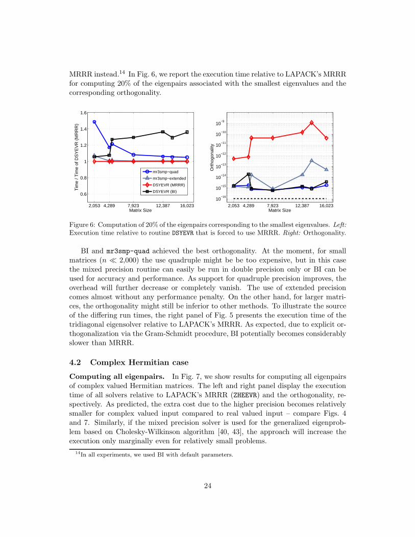
MRRR instead.14 In Fig. 6, we report the execution time relative to LAPACK’s MRRRfor computing 20% of the eigenpairs associated with the smallest eigenvalues and thecorresponding orthogonality.

2,053 4,289 7,923 12,387 16,023

0.6

0.8

1

1.2

1.4

1.6

Tim

e / T

ime

of D

SY

EV

R (

MR

RR

)

Matrix Size

mr3smp−quad

mr3smp−extended

DSYEVR (MRRR)

DSYEVR (BI)

2,053 4,289 7,923 12,387 16,023

10−16

10−15

10−14

10−13

10−12

10−11

10−10

10−9

Ort

hogo

nalit

yMatrix Size

Figure 6: Computation of 20% of the eigenpairs corresponding to the smallest eigenvalues. Left:Execution time relative to routine DSYEVR that is forced to use MRRR. Right: Orthogonality.

BI and mr3smp-quad achieved the best orthogonality. At the moment, for smallmatrices (n ≪ 2,000) the use quadruple might be be too expensive, but in this casethe mixed precision routine can easily be run in double precision only or BI can beused for accuracy and performance. As support for quadruple precision improves, theoverhead will further decrease or completely vanish. The use of extended precisioncomes almost without any performance penalty. On the other hand, for larger matri-ces, the orthogonality might still be inferior to other methods. To illustrate the sourceof the differing run times, the right panel of Fig. 5 presents the execution time of thetridiagonal eigensolver relative to LAPACK’s MRRR. As expected, due to explicit or-thogonalization via the Gram-Schmidt procedure, BI potentially becomes considerablyslower than MRRR.

4.2 Complex Hermitian case

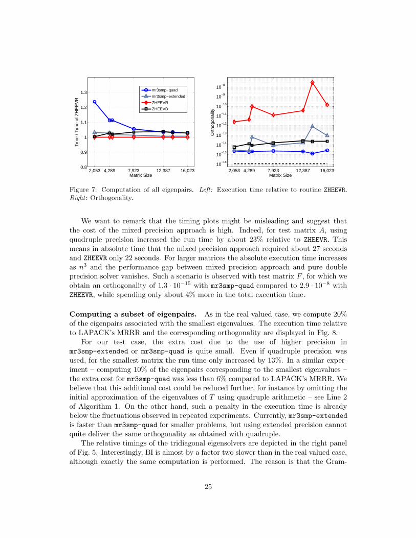
Computing all eigenpairs. In Fig. 7, we show results for computing all eigenpairsof complex valued Hermitian matrices. The left and right panel display the executiontime of all solvers relative to LAPACK’s MRRR (ZHEEVR) and the orthogonality, re-spectively. As predicted, the extra cost due to the higher precision becomes relativelysmaller for complex valued input compared to real valued input – compare Figs. 4and 7. Similarly, if the mixed precision solver is used for the generalized eigenprob-lem based on Cholesky-Wilkinson algorithm [40, 43], the approach will increase theexecution only marginally even for relatively small problems.

14In all experiments, we used BI with default parameters.

24

2,053 4,289 7,923 12,387 16,0230.8

0.9

1

1.1

1.2

1.3

Tim

e / T

ime

of Z

HE

EV

R

Matrix Size

mr3smp−quad

mr3smp−extended

ZHEEVR

ZHEEVD

2,053 4,289 7,923 12,387 16,02310

−16

10−15

10−14

10−13

10−12

10−11

10−10

10−9

10−8

Ort

hogo

nalit

y

Matrix Size

Figure 7: Computation of all eigenpairs. Left: Execution time relative to routine ZHEEVR.Right: Orthogonality.

We want to remark that the timing plots might be misleading and suggest thatthe cost of the mixed precision approach is high. Indeed, for test matrix A, usingquadruple precision increased the run time by about 23% relative to ZHEEVR. Thismeans in absolute time that the mixed precision approach required about 27 secondsand ZHEEVR only 22 seconds. For larger matrices the absolute execution time increasesas n3 and the performance gap between mixed precision approach and pure doubleprecision solver vanishes. Such a scenario is observed with test matrix F , for which weobtain an orthogonality of 1.3 · 10−15 with mr3smp-quad compared to 2.9 · 10−8 withZHEEVR, while spending only about 4% more in the total execution time.

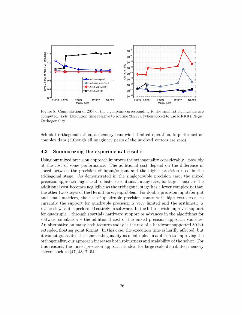
Computing a subset of eigenpairs. As in the real valued case, we compute 20%of the eigenpairs associated with the smallest eigenvalues. The execution time relativeto LAPACK’s MRRR and the corresponding orthogonality are displayed in Fig. 8.

For our test case, the extra cost due to the use of higher precision inmr3smp-extended or mr3smp-quad is quite small. Even if quadruple precision wasused, for the smallest matrix the run time only increased by 13%. In a similar exper-iment – computing 10% of the eigenpairs corresponding to the smallest eigenvalues –the extra cost for mr3smp-quad was less than 6% compared to LAPACK’s MRRR. Webelieve that this additional cost could be reduced further, for instance by omitting theinitial approximation of the eigenvalues of T using quadruple arithmetic – see Line 2of Algorithm 1. On the other hand, such a penalty in the execution time is alreadybelow the fluctuations observed in repeated experiments. Currently, mr3smp-extendedis faster than mr3smp-quad for smaller problems, but using extended precision cannotquite deliver the same orthogonality as obtained with quadruple.

The relative timings of the tridiagonal eigensolvers are depicted in the right panelof Fig. 5. Interestingly, BI is almost by a factor two slower than in the real valued case,although exactly the same computation is performed. The reason is that the Gram-

25

2,053 4,289 7,923 12,387 16,0230.7

0.8

0.9

1

1.1

1.2

Tim

e / T

ime

of Z

HE

EV

R (

MR

RR

)

Matrix Size

mr3smp−quad

mr3smp−extended

ZHEEVR (MRRR)

ZHEEVR (BI)

2,053 4,289 7,923 12,387 16,02310

−16

10−15

10−14

10−13

10−12

10−11

10−10

10−9

10−8

Ort

hogo

nalit

y

Matrix Size

Figure 8: Computation of 20% of the eigenpairs corresponding to the smallest eigenvalues arecomputed. Left: Execution time relative to routine ZHEEVR (when forced to use MRRR). Right:Orthogonality.

Schmidt orthogonalization, a memory bandwidth-limited operation, is performed oncomplex data (although all imaginary parts of the involved vectors are zero).

4.3 Summarizing the experimental results

Using our mixed precision approach improves the orthogonality considerably – possiblyat the cost of some performance. The additional cost depend on the difference inspeed between the precision of input/output and the higher precision used in thetridiagonal stage. As demonstrated in the single/double precision case, the mixedprecision approach might lead to faster executions. In any case, for larger matrices theadditional cost becomes negligible as the tridiagonal stage has a lower complexity thanthe other two stages of the Hermitian eigenproblem. For double precision input/outputand small matrices, the use of quadruple precision comes with high extra cost, ascurrently the support for quadruple precision is very limited and the arithmetic israther slow as it is performed entirely in software. In the future, with improved supportfor quadruple – through (partial) hardware support or advances in the algorithms forsoftware simulation – the additional cost of the mixed precision approach vanishes.An alternative on many architectures today is the use of a hardware supported 80-bitextended floating point format. In this case, the execution time is hardly affected, butit cannot guarantee the same orthogonality as quadruple. In addition to improving theorthogonality, our approach increases both robustness and scalability of the solver. Forthis reasons, the mixed precision approach is ideal for large-scale distributed-memorysolvers such as [47, 48, 7, 54].

26

5 Conclusions

In order to achieve improvements in accuracy, robustness, and scalability of MRRR-based eigensolvers, we take on a different perspective of the tridiagonal MRRR algo-rithm. In our perspective, given a format binary x for the input/output arguments, abinary y floating point arithmetic is used to obtain any desired (achievable) accuracy.In particular, provided the precision of the y-bit floating point format is sufficientlysmaller than the precision of the x-bit format, we obtain eigenvectors that are trulyorthogonal to input/output precision. We showed through cases studies that the per-formance, robustness, and scalability of a tridiagonal eigensolver that incorporates ourmixed precision approach can be improved by relaxing its accuracy requirements. Theapplicability of the approach depends mainly on the difference in performance betweenthe x-bit and y-bit floating point arithmetics. This is illustrated by two cases with re-spectively a small and a large gap in performance: (1) binary32 (single) input/outputwith binary64 (double) used internally and (2) binary64 input/output with binary128(quadruple) used internally.

For single precision input/output arguments, we obtain routines for dense Hermi-tian eigenproblems that are more accurate and faster, more robust, and more scalablethan the corresponding single precision eigensolver. Additionally, our mixed precisionapproach is portable and has memory requirements similar to the original. In the sin-gle precision case, the approach has no major drawback and works well for all matrixsizes, whether all eigenpairs are computed or just a subset of them.

For double precision input/output arguments, we can resort to either extended orquadruple precision. The first option offers a somewhat improved accuracy withoutmajor performance cost. The latter option provides all the benefits mentioned in thesingle precision case, but might slow down the computation due to today’s limitedsupport for quadruple precision. Nonetheless, for large matrices, the extra cost issmall even with today’s software simulated arithmetic. This is even more when onlya small subset of eigenpairs is computed and when the routines are executed in par-allel. Furthermore, if the support for quadruple precision improves in the future, themixed precision approach will – like for single precision input/output – provide higheraccuracy without any major performance penalty.

As a result, we obtain MRRR-based eigensolvers for the Hermitian eigenproblemthat are at least as accurate as other methods like the Divide-and-Conquer or the QRalgorithm while largely maintaining or even improving the strengths of MRRR: speedand scalability.

Acknowledgments

The authors would like to thank Diego Fabregat for discussion on an earlier draft ofthis report. Financial support from the Deutsche Forschungsgemeinschaft (GermanResearch Association) through grant GSC 111 is gratefully acknowledged. Enrique S.Quintana-Ortı was supported by project TIN2011-23283 and FEDER.

27

References

[1] American National Standards Institute and Institute of Electrical and Electronic Engineers.ANSI/IEEE 754-1985. 1985.

[2] E. Anderson, Z. Bai, C. Bischof, S. Blackford, J. W. Demmel, J. Dongarra, J. D. Croz, A. Green-baum, S. Hammarling, A. McKenney, and D. Sorensen. LAPACK Users’ Guide. SIAM, Philadel-phia, PA, third edition, 1999.

[3] T. Auckenthaler, V. Blum, H.-J. Bungartz, T. Huckle, R. Johanni, L. Kramer, B. Lang, H. Led-erer, and P. Willems. Parallel Solution of Partial Symmetric Eigenvalue Problems from ElectronicStructure Calculations. Parallel Comput., 37:783–794, Dec. 2011.

[4] M. Baboulin, A. Buttari, J. Dongarra, J. Kurzak, J. Langou, J. Langou, P. Luszczek, and S. To-mov. Accelerating Scientific Computations with Mixed Precision Algorithms. Computer PhysicsCommunications, 180(12):2526 – 2533, 2009.

[5] W. Barth, R. S. Martin, and J. H. Wilkinson. Calculation of the Eigenvalues of a SymmetricTridiagonal Matrix by the Method of Bisection. Numer. Math., V9(5):386–393, 1967.

[6] P. Benner, P. Ezzatti, D. Kressner, E. S. Quintana-Ortı, and A. Remon. A Mixed-PrecisionAlgorithm for the Solution of Lyapunov Equations on Hybrid CPU-GPU Platforms. ParallelComput., 37(8):439–450, Aug. 2011.

[7] P. Bientinesi, I. Dhillon, and R. van de Geijn. A Parallel Eigensolver for Dense SymmetricMatrices Based on Multiple Relatively Robust Representations. SIAM J. Sci. Comput., 27:43–66, July 2005.

[8] A. Bjorck. Iterative Refinement and Reliable Computing. In M. G. Cox and S. J. Hammarling,editors, Reliable Numerical Computation, pages 249–266, Oxford, 1990. Clarendon Press.

[9] S. Blugel, G. Bihlmeyer, D. Wortmann, C. Friedrich, M. Heide, M. Lezaic, F. Freimuth, andM. Betzinger. The Julich FLEUR Project. Julich Research Center, 1987. http://www.flapw.de.

[10] J. Cuppen. A Divide and Conquer Method for the Symmetric Tridiagonal Eigenproblem. Nu-mer. Math., 36:177–195, 1981.

[11] C. Davis and W. Kahan. The Rotation of Eigenvectors by a Perturbation. III. SIAM J. Numer.Anal., 7(1):pp. 1–46, 1970.

[12] J. W. Demmel. Applied Numerical Linear Algebra. SIAM, Philadelphia, PA, USA, 1997.

[13] J. W. Demmel, I. Dhillon, and H. Ren. On the Correctness of some Bisection-like ParallelEigenvalue Algorithms in Floating Point Arithmetic. Electronic Trans. Num. Anal., 3:116–149,1995.

[14] J. W. Demmel, J. Dongarra, A. Ruhe, and H. van der Vorst. Templates for the Solution ofAlgebraic Eigenvalue Problems: a Practical Guide. SIAM, Philadelphia, PA, USA, 2000.

[15] J. W. Demmel, Y. Hida, W. Kahan, X. S. Li, S. Mukherjee, and E. J. Riedy. Error Bounds fromExtra-Precise Iterative Refinement. ACM Trans. Math. Softw., 32(2):325–351, June 2006.

[16] J. W. Demmel, O. Marques, B. Parlett, and C. Vomel. Performance and Accuracy of LAPACK’sSymmetric Tridiagonal Eigensolvers. SIAM J. Sci. Comp., 30:1508–1526, 2008.

[17] J. W. Demmel and K. Veselic. Jacobi’s Method is more accurate than QR. SIAM J. Matrix Anal.Appl, 13:1204–1245, 1992.

[18] I. Dhillon. A New O(n2) Algorithm for the Symmetric Tridiagonal Eigenvalue/Eigenvector Prob-lem. PhD thesis, EECS Department, University of California, Berkeley, 1997.

[19] I. Dhillon. Current Inverse Iteration Software Can Fail. BIT, 38:685–704, 1998.

[20] I. Dhillon and B. Parlett. Multiple Representations to Compute Orthogonal Eigenvectors ofSymmetric Tridiagonal Matrices. Linear Algebra Appl., 387:1–28, 2004.

28

[21] I. Dhillon and B. Parlett. Orthogonal Eigenvectors and Relative Gaps. SIAM J. MatrixAnal. Appl., 25:858–899, 2004.

[22] I. Dhillon, B. Parlett, and C. Vomel. Glued Matrices and the MRRR Algorithm. SIAM J. Sci.Comput, 27:496–510, 2005.

[23] I. Dhillon, B. Parlett, and C. Vomel. The Design and Implementation of the MRRR Algorithm.ACM Trans. Math. Software, 32:533–560, December 2006.

[24] J. Dongarra, J. Du Cruz, I. Duff, and S. Hammarling. A Set of Level 3 Basic Linear AlgebraSubprograms. ACM Trans. Math. Software, 16:1–17, 1990.

[25] J. Dongarra and D. C. Sorensen. A fully parallel algorithm for the symmetric eigenvalue problem.SIAM J. Sci. Stat. Comput., 8(2):139–154, Mar. 1987.

[26] G. Fann, R. Littlefield, and D. Elwood. Performance of a Fully Parallel Dense Real SymmetricEigensolver in Quantum Chemistry Applications. In Proceedings of High Performance Computing’95, Simulation MultiConference. The Society for Computer Simulation, 1995.

[27] J. Francis. The QR Transform - A Unitary Analogue to the LR Transformation, Part I and II.The Comp. J., 4, 1961/1962.

[28] G. H. Golub and C. F. V. Loan. Matrix Computations. The Johns Hopkins University Press, 3rdedition, 1996.

[29] M. Gu and S. C. Eisenstat. A Divide-and-Conquer Algorithm for the Symmetric TridiagonalEigenproblem. SIAM J. Matrix Anal. Appl., 16(1):172–191, 1995.

[30] N. Higham. Iterative Refinement for Linear Systems and LAPACK. IMA Journal of NumericalAnalysis, 17(4):495–509, 1997.

[31] IEEE Computer Society. IEEE Standard for Floating-Point Arithmetic. IEEE Standard 754-2008,2008.

[32] C. G. J. Jacobi. Uber ein leichtes Verfahren die in der Theorie der Sacularstorungen vorkom-menden Gleichungen numerisch aufzulosen. 30:51–94, 1846.

[33] W. Kahan. Lecture Notes on the Status of IEEE Standard 754 for Binary Floating-Point Arith-metic. Manuscript, 1997.

[34] D. Kressner. Numerical Methods for General And Structured Eigenvalue Problems. Springer,Berlin Heidelberg New York, 2005.

[35] V. Kublanovskaya. On some Algorithms for the Solution of the Complete Eigenvalue Problem.Zh. Vych. Mat., 1:555–572, 1961.

[36] X. S. Li, J. W. Demmel, D. H. Bailey, G. Henry, Y. Hida, J. Iskandar, W. Kahan, A. Kapur,M. C. Martin, T. Tung, and D. J. Yoo. Design, Implementation and Testing of Extended andMixed Precision BLAS. ACM Trans. Math. Software, 28:2002, 2002.

[37] O. Marques, B. Parlett, and C. Vomel. Computations of Eigenpair Subsets with the MRRRAlgorithm. Numerical Linear Algebra with Applications, 13(8):643–653, 2006.

[38] O. Marques, E. Riedy, and C. Vomel. Benefits of IEEE-754 Features in Modern SymmetricTridiagonal Eigensolvers. SIAM J. Sci. Comput., 28:1613–1633, September 2006.

[39] O. A. Marques, C. Vomel, J. W. Demmel, and B. N. Parlett. Algorithm 880: A Testing Infras-tructure for Symmetric Tridiagonal Eigensolvers. ACM Trans. Math. Softw., 35(1):8:1–8:13, July2008.

[40] R. Martin and J. Wilkinson. Reduction of the Symmetric Eigenproblem Ax = λBx; and RelatedProblems to Standard Form. Numerische Mathematik, 11:99–110, 1968. 10.1007/BF02165306.

[41] C. B. Moler. Iterative Refinement in Floating Point. J. ACM, 14(2):316–321, Apr. 1967.

[42] M. Nakata. The MPACK (MBLAS / MLAPACK): A Multiple Precision Arithmetic Version ofBLAS and LAPACK, 2012. http://mplapack.sourceforge.net.

29

[43] B. Parlett. The Symmetric Eigenvalue Problem. Prentice-Hall, Inc., Upper Saddle River, NJ,USA, 1998.

[44] B. Parlett and I. Dhillon. Fernando’s Solution to Wilkinson’s Problem: an Application of DoubleFactorization. Linear Algebra Appl., 267:247–279, 1996.

[45] B. Parlett and I. Dhillon. Relatively Robust Representations of Symmetric Tridiagonals. LinearAlgebra Appl., 309(1-3):121 – 151, 2000.

[46] B. Parlett and O. Marques. An Implementation of the DQDS Algorithm (Positive Case). LinearAlgebra Appl., 309:217–259, 1999.

[47] M. Petschow and P. Bientinesi. MR3-SMP: A Symmetric Tridiagonal Eigensolver for Multi-CoreArchitectures. Parallel Computing, 37(12):795 – 805, 2011.

[48] M. Petschow, E. Peise, and P. Bientinesi. High-Performance Solvers For Dense HermitianEigenproblems. Submitted, 2011.

[49] A. Sameh. On Jacobi and Jacobi-like Algorithms for a Parallel Computer. Math. Comp.,25(115):579–590, 1971.

[50] M. Sears, K. Stanley, and G. Henry. Application of a High Performance Parallel Eigensolverto Electronic Structure Calculations. In Proceedings of the 1998 ACM/IEEE conference on Su-percomputing (CDROM), Supercomputing ’98, pages 1–1, Washington, DC, USA, 1998. IEEEComputer Society.

[51] W. Stein et al. Sage Mathematics Software. The Sage Development Team, 2012.http://www.sagemath.org.

[52] F. G. Van Zee, R. van de Geijn, and G. Quintana-Orti. Restructuring the QR Algorithm forHigh-Performance Application of Givens Rotations. Technical Report TR-11-36, The Universityof Texas at Austin, Department of Computer Sciences, October 2011.

[53] C. Vomel. A Refined Representation Tree for MRRR. LAPACK Working Note 194, Departmentof Computer Science, University of Tennessee, Knoxville, Nov. 2007.

[54] C. Vomel. ScaLAPACK’s MRRR Algorithm. ACM Trans. Math. Software, 37:1:1–1:35, January2010.

[55] J. H. Wilkinson. The Calculation of the Eigenvectors of Codiagonal Matrices. Comp. J., 1(2):90–96, 1958.

[56] P. Willems. On MR3-type Algorithms for the Tridiagonal Symmetric Eigenproblem and BidiagonalSVD. PhD thesis, University of Wuppertal, 2010.

[57] P. Willems and B. Lang. Block Factorizations and qd-type Transformations for the MR3 Algo-rithm. Electron. Trans. Numer. Anal., 38:363–400, 2011.

[58] S. Wolfram. Mathematica - a system for doing mathematics by computer (2. ed.). Addison-Wesley,1992.

30