Improved Transportation Networks Facilitate Adaptation to Pollutionand Temperature ExtremesPanle Jia Barwicka,c, Dave Donaldsonb,c,1, Shanjun Lia,c, Yatang Lind, and Deyu Raoa

aCornell University, Ithaca, NY 14853, USA; bMassachusetts Institute of Technology, Cambridge, MA 02139, USA; cNational Bureau ofEconomic Research, Cambridge, MA 02138, USA; dHong Kong University of Science and Technology, Clear Water Bay, Hong Kong

This manuscript was compiled on May 13, 2021

The social costs of air pollution and climate change hinge critically on humans’ ability to adapt. Based on high-resolution transaction records from the world’s largest payment network, this research shows how China’s rapidexpansion of high-speed railways and air-travel networks (HSR/air) has facilitated the use of intercity travel asan effective means of adaptation. On average, HSR/air connection would reduce travelers’ exposure to bothextreme pollution and temperature by 16% when home cities are experiencing pollution and temperature ex-tremes. Longer-horizon changes in travel patterns before and after HSR/air access explain 56% of the reductionin pollution exposure and 81% for temperature exposure. Contemporaneous responses to unexpected adverseconditions account for the remaining impact. These reductions in exposure to environmental extremes entailsubstantial health benefits. This study contributes to our understanding of the role of adaptation and the benefitof transportation infrastructure investment in a changing environment.

Climate Change | Transportation Infrastructure | Temperature shocks | Air Pollution | Adaptation

A ir pollution and climate change are among the most pressing environmental challenges of our time.These challenges impose large social costs by affecting economic growth,1, 2, 3 social stability,4, 5 and

health.6, 7, 8, 9 The social costs of climate change and air pollution depend crucially on the extent to whichhumans can adapt to extreme environmental conditions. While long-term migration can be an effectivestrategy for adaptation to a changing environment,10, 11, 12, 13 it entails significant costs especially for residentsin developing countries with severe market frictions and institutional constraints. In contrast, short-termintercity travel may offer a more practical and affordable adaptation strategy to reduce the negativeeffects of local environmental conditions. Indeed, “haze-avoidance tourism” and “smog refugees” havebecome important new themes in intercity travel in China with the advent of cheap and fast transportationmodes.14, 15, 16

This study provides the first analysis of how improved transportation infrastructure facilitates behavioralchanges in response to adverse environmental conditions. We do so in the context of China’s rapidexpansion of high-speed-railways (HSR) and air-travel networks (“air"). Since 2008, China has extendedHSR dramatically to a total length of over 29,000 km by the end of 2018, twice as long as the HSR networksof all other countries combined (Panel (a) of Figure S1 in Supplementary Information (SI)). China’s airnetwork has also grown considerably, with the number of direct flights nearly doubling between 2011 and2016 (Panels (b) and (c) of Figure S1). Our analysis uses the first high-frequency (daily) measure of travelerflows between all city-pairs in China and compares the intensity of extreme air pollution and temperaturethat is actually realized by travelers from cities with HSR/air access to that by travelers without such access.An estimate of the causal effect is established based on the day-to-day variation in travel patterns and theexpansion of HSR and air networks.

Data and Descriptive EvidenceOur primary data source is the universe of credit- and debit-card transactions made through UnionPay, theonly inter-bank payment network in China and the largest payment network in the world. We constructcross-city travel between all city pairs during 2013-2016 using offline transactions where the cardholder is

1

physically present at the merchant’s location. We then merge this daily travel data with daily air pollutionand temperature readings at the city level, as well as data on the HSR and air network expansion over time.The outcome variables of interest in our analysis measure the realized exposure to pollution (and, separately,to temperature extremes) among travelers, constructed on the basis of the environmental conditions at theirdestination cities. Such a measure cannot be constructed without the high-frequency and high-spatial traveland environmental data merge that we develop here. Table S1 and Section A in SI provide the summarystatistics of key variables and further details on data sets used in this analysis.

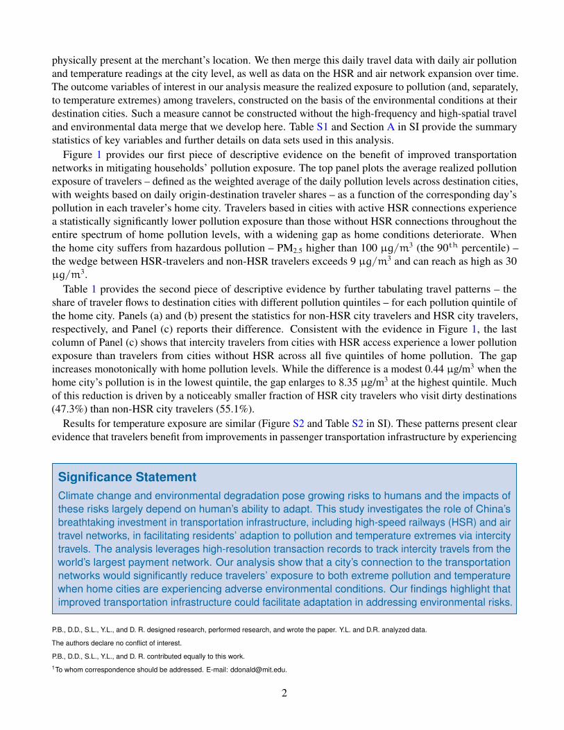
Figure 1 provides our first piece of descriptive evidence on the benefit of improved transportationnetworks in mitigating households’ pollution exposure. The top panel plots the average realized pollutionexposure of travelers – defined as the weighted average of the daily pollution levels across destination cities,with weights based on daily origin-destination traveler shares – as a function of the corresponding day’spollution in each traveler’s home city. Travelers based in cities with active HSR connections experiencea statistically significantly lower pollution exposure than those without HSR connections throughout theentire spectrum of home pollution levels, with a widening gap as home conditions deteriorate. Whenthe home city suffers from hazardous pollution – PM2.5 higher than 100 µg/m3 (the 90th percentile) –the wedge between HSR-travelers and non-HSR travelers exceeds 9 µg/m3 and can reach as high as 30µg/m3.

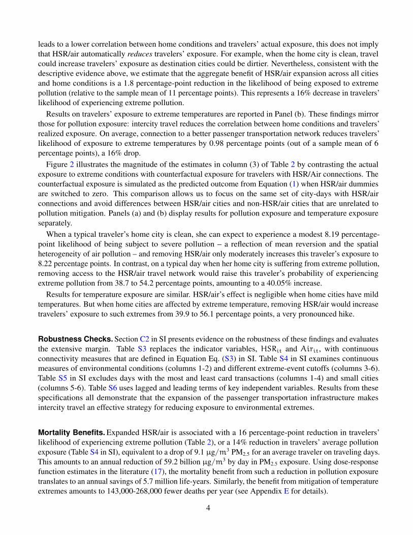
Table 1 provides the second piece of descriptive evidence by further tabulating travel patterns – theshare of traveler flows to destination cities with different pollution quintiles – for each pollution quintile ofthe home city. Panels (a) and (b) present the statistics for non-HSR city travelers and HSR city travelers,respectively, and Panel (c) reports their difference. Consistent with the evidence in Figure 1, the lastcolumn of Panel (c) shows that intercity travelers from cities with HSR access experience a lower pollutionexposure than travelers from cities without HSR across all five quintiles of home pollution. The gapincreases monotonically with home pollution levels. While the difference is a modest 0.44 µg/m3 when thehome city’s pollution is in the lowest quintile, the gap enlarges to 8.35 µg/m3 at the highest quintile. Muchof this reduction is driven by a noticeably smaller fraction of HSR city travelers who visit dirty destinations(47.3%) than non-HSR city travelers (55.1%).

Results for temperature exposure are similar (Figure S2 and Table S2 in SI). These patterns present clearevidence that travelers benefit from improvements in passenger transportation infrastructure by experiencing

Significance StatementClimate change and environmental degradation pose growing risks to humans and the impacts ofthese risks largely depend on human’s ability to adapt. This study investigates the role of China’sbreathtaking investment in transportation infrastructure, including high-speed railways (HSR) and airtravel networks, in facilitating residents’ adaption to pollution and temperature extremes via intercitytravels. The analysis leverages high-resolution transaction records to track intercity travels from theworld’s largest payment network. Our analysis show that a city’s connection to the transportationnetworks would significantly reduce travelers’ exposure to both extreme pollution and temperaturewhen home cities are experiencing adverse environmental conditions. Our findings highlight thatimproved transportation infrastructure could facilitate adaptation in addressing environmental risks.

P.B., D.D., S.L., Y.L., and D. R. designed research, performed research, and wrote the paper. Y.L. and D.R. analyzed data.

The authors declare no conflict of interest.

P.B., D.D., S.L., Y.L., and D. R. contributed equally to this work.1To whom correspondence should be addressed. E-mail: ddonald@mit.edu.

2

reduced exposure to adverse environmental conditions.

Regression ModelTo quantify the benefit of improved transportation infrastructure in mitigating pollution, we follow thestandard difference-in-differences strategy in a panel regression framework:

TravExpoit = β1 Expoit + β2 HSRit × Expoit + β3i × HSRit + µi + δt + εit. [1]

In this expression, Expoit measures pollution exposure in city i at time t, which we construct as a simpleindicator that equals one whenever i experiences extreme pollution (PM2.5 > 100µg/m3, the 90th percentileof the empirical distribution).* The dependent variable, TravExpoit, analogously measures the pollutionexposure at time t of travelers whose home city is i. We calculate this from the extreme pollution that wasrealized in the destination cities that each traveler from city i visited at time t; see Equation (S1).

The variable HSRit is an indicator set equal to one if city i has direct access to the HSR network attime t. We let the impact of HSR access on travelers’ pollution exposure be a function of both the homecity’s exposure (captured in the coefficient β2) and the identity of the home city itself (via the set ofcoefficients β3i, one for each city i). Finally, all regressions control for city fixed effects µi, which capturetime-invariant city-level unobservables that affect travelers’ exposure (e.g. economic connections withother cities), as well as year-day (i.e. day-of-sample) fixed effects δt that control for phenomena such asholidays and seasonality.

We estimate the total benefit of the expansion of the HSR network on travelers’ pollution exposure by−∑

i,tωi,t(β2 × Expoit + β3i), where ωi,t is the city-i and day-t share of travelers among all HSRcity-days in our sample period. All regressions are weighted by the number of home city i’s travelers attime t, so that the effect sizes reported below can be interpreted as the national average across all travel.

We also present two variants on specification 1. First, we include an indicator for airport access in city iat time t, denoted Airit, both instead of and in addition to the variable HSRit. This allows us to comparethe benefits of rail and air travel infrastructure. Second, we study temperature exposure analogously topollution exposure by letting Expoit take the value one if city i at time t experiences extreme temperature(daily temperature > 90◦F or < 30◦F) and adjusting TravExpoit accordingly.†

Section C of SI presents more details about our regression framework and examines alternative cutoffsfor extreme pollution and temperature conditions.

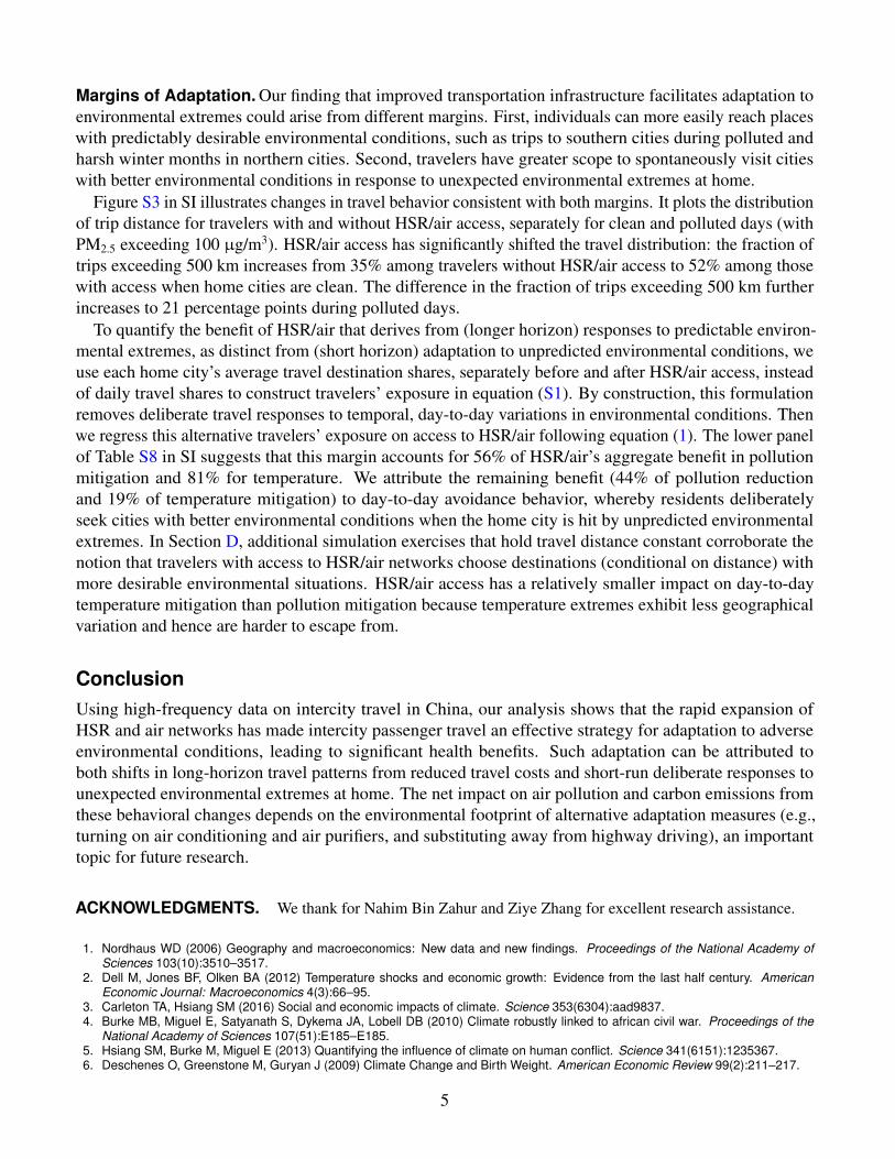
Empirical ResultsPanel (a) of Table 2 reports OLS estimates as specified in Equation (1). Columns (1)-(3) examine the effectson travelers’ pollution exposure from obtaining access to HSR, air, and both, respectively. The estimates ofβ1 in all columns are much lower than one and vary from 0.19 to 0.27, implying that intercity travel reducessubstantially the correlation between home pollution and travelers’ realized exposure. The estimates ofβ2 are negative, significant and economically large in all columns, suggesting that improvements in thetransportation network (both HSR and air) can change travel patterns in a way that further flattens therelationship between home extreme pollution and travelers’ exposure.‡

We summarize HSR/air’s aggregate benefit, −∑

i,tωi,t{β2 × Expoit + β3i}, in the last row of panel(a). In theory, its sign is ambiguous. While HSR/air expansion allows individuals to visit further places and

*China’s Ministry of Ecology and Environment’s standard for daily maximum PM2.5 is 75 µg/m3. In comparison, in the U.S. the Environ-mental Protection Agency’s daily PM2.5 standard is 35 µg/m3.

†Using 30◦F and 90◦F as cutoffs, extreme temperature occurs in around 10% of city-days.‡The estimate for β2 is -0.05 for HSR and -0.14 for Air, respectively, largely because air travel spans a longer distance and the spatialcorrelation of pollution decays with distance.

3

leads to a lower correlation between home conditions and travelers’ actual exposure, this does not implythat HSR/air automatically reduces travelers’ exposure. For example, when the home city is clean, travelcould increase travelers’ exposure as destination cities could be dirtier. Nevertheless, consistent with thedescriptive evidence above, we estimate that the aggregate benefit of HSR/air expansion across all citiesand home conditions is a 1.8 percentage-point reduction in the likelihood of being exposed to extremepollution (relative to the sample mean of 11 percentage points). This represents a 16% decrease in travelers’likelihood of experiencing extreme pollution.

Results on travelers’ exposure to extreme temperatures are reported in Panel (b). These findings mirrorthose for pollution exposure: intercity travel reduces the correlation between home conditions and travelers’realized exposure. On average, connection to a better passenger transportation network reduces travelers’likelihood of exposure to extreme temperatures by 0.98 percentage points (out of a sample mean of 6percentage points), a 16% drop.

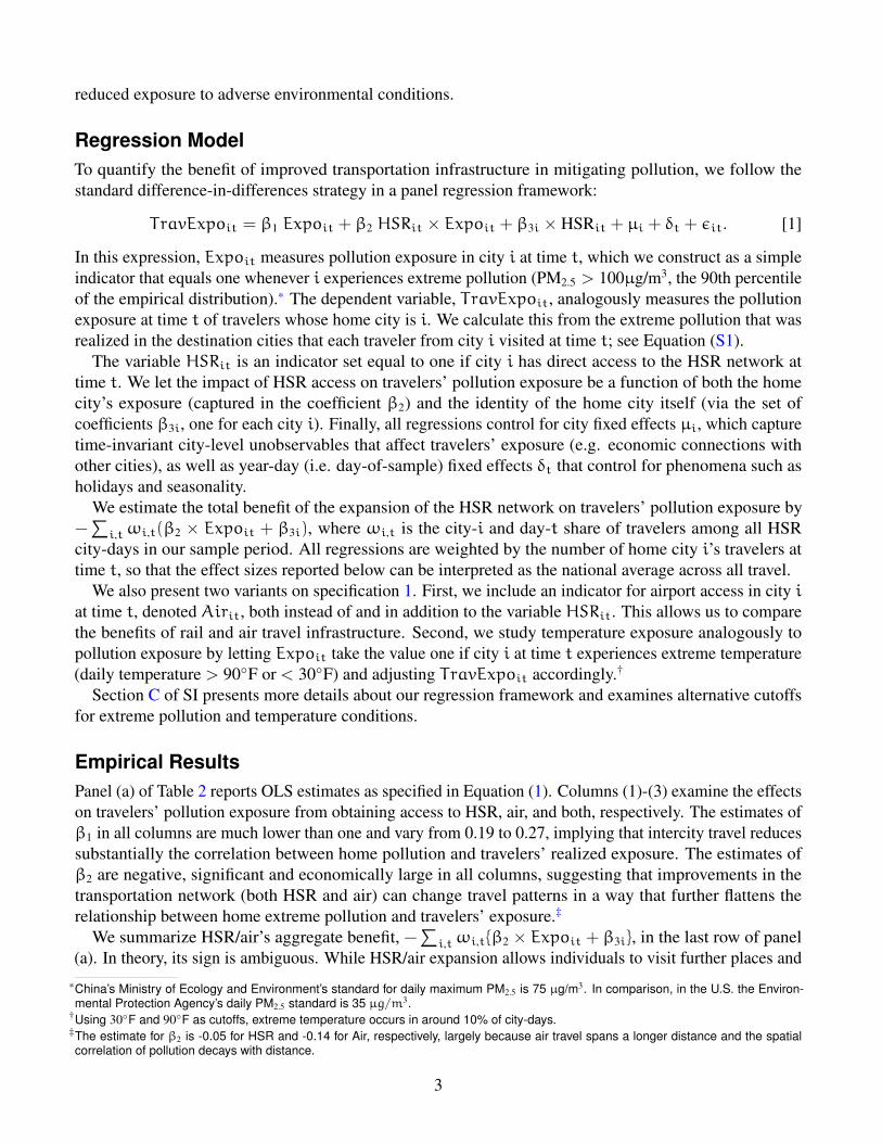
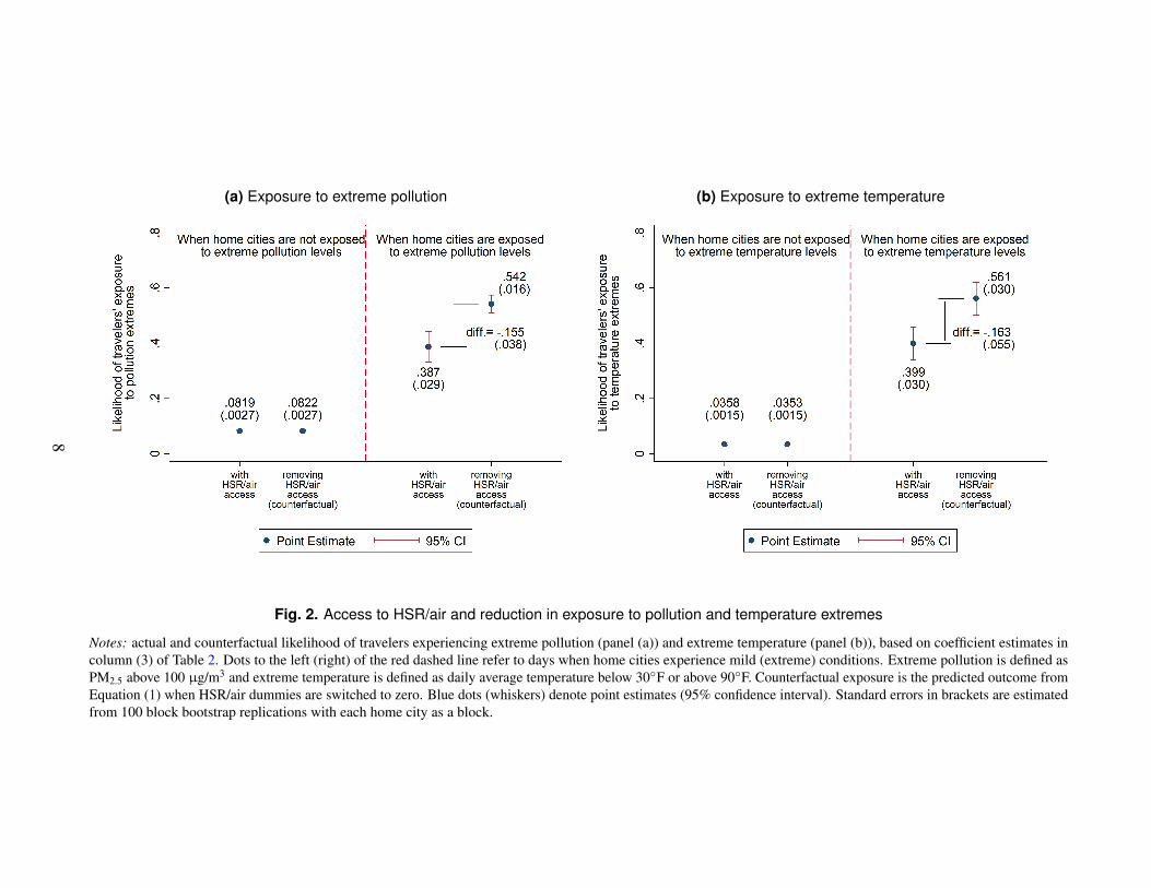
Figure 2 illustrates the magnitude of the estimates in column (3) of Table 2 by contrasting the actualexposure to extreme conditions with counterfactual exposure for travelers with HSR/Air connections. Thecounterfactual exposure is simulated as the predicted outcome from Equation (1) when HSR/air dummiesare switched to zero. This comparison allows us to focus on the same set of city-days with HSR/airconnections and avoid differences between HSR/air cities and non-HSR/air cities that are unrelated topollution mitigation. Panels (a) and (b) display results for pollution exposure and temperature exposureseparately.

When a typical traveler’s home city is clean, she can expect to experience a modest 8.19 percentage-point likelihood of being subject to severe pollution – a reflection of mean reversion and the spatialheterogeneity of air pollution – and removing HSR/air only moderately increases this traveler’s exposure to8.22 percentage points. In contrast, on a typical day when her home city is suffering from extreme pollution,removing access to the HSR/air travel network would raise this traveler’s probability of experiencingextreme pollution from 38.7 to 54.2 percentage points, amounting to a 40.05% increase.

Results for temperature exposure are similar. HSR/air’s effect is negligible when home cities have mildtemperatures. But when home cities are affected by extreme temperature, removing HSR/air would increasetravelers’ exposure to such extremes from 39.9 to 56.1 percentage points, a very pronounced hike.

Robustness Checks. Section C2 in SI presents evidence on the robustness of these findings and evaluatesthe extensive margin. Table S3 replaces the indicator variables, HSRit and Airit, with continuousconnectivity measures that are defined in Equation Eq. (S3) in SI. Table S4 in SI examines continuousmeasures of environmental conditions (columns 1-2) and different extreme-event cutoffs (columns 3-6).Table S5 in SI excludes days with the most and least card transactions (columns 1-4) and small cities(columns 5-6). Table S6 uses lagged and leading terms of key independent variables. Results from thesespecifications all demonstrate that the expansion of the passenger transportation infrastructure makesintercity travel an effective strategy for reducing exposure to environmental extremes.

Mortality Benefits. Expanded HSR/air is associated with a 16 percentage-point reduction in travelers’likelihood of experiencing extreme pollution (Table 2), or a 14% reduction in travelers’ average pollutionexposure (Table S4 in SI), equivalent to a drop of 9.1 µg/m3 PM2.5 for an average traveler on traveling days.This amounts to an annual reduction of 59.2 billion µg/m3 by day in PM2.5 exposure. Using dose-responsefunction estimates in the literature (17), the mortality benefit from such a reduction in pollution exposuretranslates to an annual savings of 5.7 million life-years. Similarly, the benefit from mitigation of temperatureextremes amounts to 143,000-268,000 fewer deaths per year (see Appendix E for details).

4

Margins of Adaptation. Our finding that improved transportation infrastructure facilitates adaptation toenvironmental extremes could arise from different margins. First, individuals can more easily reach placeswith predictably desirable environmental conditions, such as trips to southern cities during polluted andharsh winter months in northern cities. Second, travelers have greater scope to spontaneously visit citieswith better environmental conditions in response to unexpected environmental extremes at home.

Figure S3 in SI illustrates changes in travel behavior consistent with both margins. It plots the distributionof trip distance for travelers with and without HSR/air access, separately for clean and polluted days (withPM2.5 exceeding 100 µg/m3). HSR/air access has significantly shifted the travel distribution: the fraction oftrips exceeding 500 km increases from 35% among travelers without HSR/air access to 52% among thosewith access when home cities are clean. The difference in the fraction of trips exceeding 500 km furtherincreases to 21 percentage points during polluted days.

To quantify the benefit of HSR/air that derives from (longer horizon) responses to predictable environ-mental extremes, as distinct from (short horizon) adaptation to unpredicted environmental conditions, weuse each home city’s average travel destination shares, separately before and after HSR/air access, insteadof daily travel shares to construct travelers’ exposure in equation (S1). By construction, this formulationremoves deliberate travel responses to temporal, day-to-day variations in environmental conditions. Thenwe regress this alternative travelers’ exposure on access to HSR/air following equation (1). The lower panelof Table S8 in SI suggests that this margin accounts for 56% of HSR/air’s aggregate benefit in pollutionmitigation and 81% for temperature. We attribute the remaining benefit (44% of pollution reductionand 19% of temperature mitigation) to day-to-day avoidance behavior, whereby residents deliberatelyseek cities with better environmental conditions when the home city is hit by unpredicted environmentalextremes. In Section D, additional simulation exercises that hold travel distance constant corroborate thenotion that travelers with access to HSR/air networks choose destinations (conditional on distance) withmore desirable environmental situations. HSR/air access has a relatively smaller impact on day-to-daytemperature mitigation than pollution mitigation because temperature extremes exhibit less geographicalvariation and hence are harder to escape from.

ConclusionUsing high-frequency data on intercity travel in China, our analysis shows that the rapid expansion ofHSR and air networks has made intercity passenger travel an effective strategy for adaptation to adverseenvironmental conditions, leading to significant health benefits. Such adaptation can be attributed toboth shifts in long-horizon travel patterns from reduced travel costs and short-run deliberate responses tounexpected environmental extremes at home. The net impact on air pollution and carbon emissions fromthese behavioral changes depends on the environmental footprint of alternative adaptation measures (e.g.,turning on air conditioning and air purifiers, and substituting away from highway driving), an importanttopic for future research.

ACKNOWLEDGMENTS. We thank for Nahim Bin Zahur and Ziye Zhang for excellent research assistance.

1. Nordhaus WD (2006) Geography and macroeconomics: New data and new findings. Proceedings of the National Academy ofSciences 103(10):3510–3517.

2. Dell M, Jones BF, Olken BA (2012) Temperature shocks and economic growth: Evidence from the last half century. AmericanEconomic Journal: Macroeconomics 4(3):66–95.

3. Carleton TA, Hsiang SM (2016) Social and economic impacts of climate. Science 353(6304):aad9837.4. Burke MB, Miguel E, Satyanath S, Dykema JA, Lobell DB (2010) Climate robustly linked to african civil war. Proceedings of the

National Academy of Sciences 107(51):E185–E185.5. Hsiang SM, Burke M, Miguel E (2013) Quantifying the influence of climate on human conflict. Science 341(6151):1235367.6. Deschenes O, Greenstone M, Guryan J (2009) Climate Change and Birth Weight. American Economic Review 99(2):211–217.

5

7. Currie J, Neidell M (2005) Air pollution and infant health: What can we learn from california’s recent experience. Quarterly Journalof Economics 120:1003–1030.

8. Chen Y, Ebenstein A, Greenstone M, Li H (2013) Evidence on the impact of sustained exposure to air pollution on life expectancyfrom china’s huai river policy. Proceedings of the National Academy of Sciences 110(32):12936–12941.

9. Landrigan P, et al. (2018) The lancet commission on pollution and health. The Lancet 391(10119):462–512.10. Banzhaf HS, Walsh RP (2008) Do people vote with their feet? an empirical test of tiebout. American Economic Review 98(3):843–

863.11. Deschenes O, Moretti E (2009) Extreme weather events, mortality, and migration. The Review of Economics and Statistics

91(4):659–681.12. Kahn M (2010) Climatopolis: How Our Cities will Thrive in Our Hotter Future. (Basic Books).13. Freeman R, Liang W, Song R, Timmins C (2019) Willingness to pay for clean air in china. Journal of Environmental Economics

and Management 94:188–216.14. Arlt WG (2017) As smog hits china, chinese tourists seek fresh air on pollution free holidays. Forbes.15. Sharkov D (2016) Smog in china prompts tide of tourism fleeing ’airpocalypse:’ report. Newsweek.16. Chen S, Chen Y, Lei Z, Tan-Soo JS (2021) Chasing clean air: Pollution-induced travels in china. Journal of the Association of

Environmental and Resource Economists pp. 59–89.17. Ebenstein A, Fan M, Greenstone M, He G, Zhou M (2017) New evidence on the impact of sustained exposure to air pollution on

life expectancy from china’s huai river policy. Proceedings of the National Academy of Sciences 114(39):10384–10389.18. Zhang J, Mu Q (2018) Air pollution and defensive expenditures: Evidence from particulate-filtering facemasks. Journal of Environ-

mental Economics and Management 92:517–536.19. Ito K, Zhang S (2020) Willingness to pay for clean air: Evidence from air purifier markets in china. Journal of Political Economy

128:1627–1672.20. Zheng S, Kahn ME (2017) A new era of pollution progress in urban china? Journal of Economic Perspectives 31(1):71–92.21. Kahn ME, Zheng S (2016) Blue skies over Beijing: Economic growth and the environment in China. (Princeton University Press).22. Barwick PJ, Li S, Lin L, Zou E (2020) From fog to smog: the value of pollution information.23. Li S, Liu Y, Purevjav AO, Yang L (2019) Does subway expansion improve air quality? Journal of Environmental Economics and

Management.

6

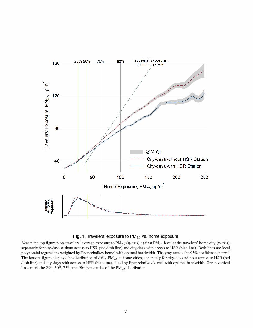
Fig. 1. Travelers’ exposure to PM2.5 vs. home exposureNotes: the top figure plots travelers’ average exposure to PM2.5 (y-axis) against PM2.5 level at the travelers’ home city (x-axis),separately for city-days without access to HSR (red dash line) and city-days with access to HSR (blue line). Both lines are localpolynomial regressions weighted by Epanechnikov kernel with optimal bandwidth. The gray area is the 95% confidence interval.The bottom figure displays the distribution of daily PM2.5 at home cities, separately for city-days without access to HSR (reddash line) and city-days with access to HSR (blue line), fitted by Epanechnikov kernel with optimal bandwidth. Green verticallines mark the 25th, 50th, 75th, and 90th percentiles of the PM2.5 distribution.

7

(a) Exposure to extreme pollution (b) Exposure to extreme temperature

Fig. 2. Access to HSR/air and reduction in exposure to pollution and temperature extremes

Notes: actual and counterfactual likelihood of travelers experiencing extreme pollution (panel (a)) and extreme temperature (panel (b)), based on coefficient estimates incolumn (3) of Table 2. Dots to the left (right) of the red dashed line refer to days when home cities experience mild (extreme) conditions. Extreme pollution is defined asPM2.5 above 100 µg/m3 and extreme temperature is defined as daily average temperature below 30◦F or above 90◦F. Counterfactual exposure is the predicted outcome fromEquation (1) when HSR/air dummies are switched to zero. Blue dots (whiskers) denote point estimates (95% confidence interval). Standard errors in brackets are estimatedfrom 100 block bootstrap replications with each home city as a block.

8

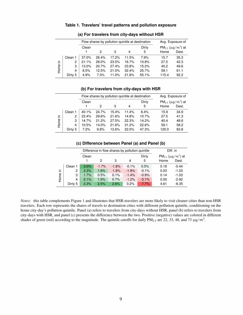
Table 1. Travelers’ travel patterns and pollution exposure

(a) For travelers from city-days without HSR

Flow shares by pollution quintile at destination Avg. Exposure of

Clean Dirty PM2.5 (µg/m3) at1 2 3 4 5 Home Dest.

Hom

ein

Clean 1 37.0% 26.4% 17.2% 11.5% 7.9% 15.7 35.32 21.1% 28.0% 23.5% 16.7% 10.8% 27.5 42.33 13.0% 20.7% 27.4% 23.8% 15.2% 40.2 49.64 8.5% 12.5% 21.0% 32.4% 25.7% 59.1 61.1

Dirty 5 4.9% 7.3% 11.0% 21.8% 55.1% 115.4 92.2

(b) For travelers from city-days with HSR

Flow shares by pollution quintile at destination Avg. Exposure of

Clean Dirty PM2.5 (µg/m3) at1 2 3 4 5 Home Dest.

Hom

ein

Clean 1 40.1% 24.7% 15.4% 11.4% 8.4% 15.9 34.92 23.4% 29.6% 21.6% 14.8% 10.7% 27.5 41.33 14.7% 21.2% 27.5% 22.3% 14.2% 40.4 48.64 10.5% 14.0% 21.6% 31.2% 22.6% 59.1 58.2

Dirty 5 7.2% 9.8% 13.6% 22.0% 47.3% 120.0 83.8

(c) Difference between Panel (a) and Panel (b)

Difference in flow shares by pollution quintile Diff. in

Clean Dirty PM2.5 (µg/m3) at1 2 3 4 5 Home Dest.

Hom

ein

Clean 1 3.0% -1.7% -1.8% -0.1% 0.5% 0.18 -0.442 2.3% 1.6% -1.8% -1.9% -0.1% 0.03 -1.033 1.7% 0.5% 0.1% -1.4% -0.9% 0.14 -1.034 2.1% 1.5% 0.7% -1.2% -3.1% 0.00 -2.92

Dirty 5 2.3% 2.5% 2.6% 0.2% -7.7% 4.61 -8.35

Notes: this table complements Figure 1 and illustrates that HSR-travelers are more likely to visit cleaner cities than non-HSRtravelers. Each row represents the shares of travels to destination cities with different pollution quintile, conditioning on thehome city-day’s pollution quintile. Panel (a) refers to travelers from city-days without HSR, panel (b) refers to travelers fromcity-days with HSR, and panel (c) presents the difference between the two. Positive (negative) values are colored in differentshades of green (red) according to the magnitude. The quintile cutoffs for daily PM2.5 are 22, 33, 48, and 73 µg/m3.

9

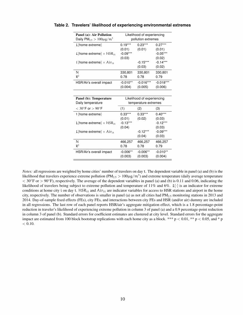
Table 2. Travelers’ likelihood of experiencing environmental extremes

Panel (a): Air Pollution Likelihood of experiencingDaily PM2.5 > 100µg/m3 pollution extremes

1{home extreme} 0.19*** 0.23*** 0.27***(0.01) (0.01) (0.01)

1{home extreme}×HSRit -0.09*** -0.05***(0.03) (0.02)

1{home extreme}×Airit -0.15*** -0.14***(0.03) (0.02)

N 330,801 330,801 330,801R2 0.78 0.78 0.79

HSR/Air’s overall impact -0.010** -0.016*** -0.018***(0.004) (0.005) (0.006)

Panel (b): Temperature Likelihood of experiencingDaily temperature temperature extremes

< 30◦F or > 90◦F (1) (2) (3)

1{home extreme} 0.33*** 0.33*** 0.40***(0.01) (0.02) (0.03)

1{home extreme}×HSRit -0.13*** -0.12***(0.04) (0.03)

1{home extreme}×Airit -0.12*** -0.09***(0.04) (0.03)

N 466,257 466,257 466,257R2 0.78 0.78 0.79

HSR/Air’s overall impact -0.006** -0.006** -0.010**(0.003) (0.003) (0.004)

Notes: all regressions are weighted by home cities’ number of travelers on day t. The dependent variable in panel (a) and (b) is thelikelihood that travelers experience extreme pollution (PM2.5 > 100µg/m3) and extreme temperature (daily average temperature< 30◦F or > 90◦F), respectively. The average of the dependent variables in panel (a) and (b) is 0.11 and 0.06, indicating thelikelihood of travelers being subject to extreme pollution and temperature of 11% and 6%. 1{·} is an indicator for extremeconditions at home city i on day t. HSRit and Airit are indicator variables for access to HSR stations and airport in the homecity, respectively. The number of observations is smaller in panel (a) as not all cities had PM2.5 monitoring stations in 2013 and2014. Day-of-sample fixed effects (FEs), city FEs, and interactions between city FEs and HSR (and/or air) dummy are includedin all regressions. The last row of each panel reports HSR/air’s aggregate mitigation effect, which is a 1.8 percentage-pointreduction in traveler’s likelihood of experiencing extreme pollution in column 3 of panel (a) and a 0.9 percentage-point reductionin column 3 of panel (b). Standard errors for coefficient estimates are clustered at city level. Standard errors for the aggregateimpact are estimated from 100 block bootstrap replications with each home city as a block. *** p < 0.01, ** p < 0.05, and * p< 0.10.

10

Supplementary InformationThis study provides the first analysis of how transportation infrastructure promotes short-term mobility and facilitatesbehavioral changes in response to adverse environmental conditions, in the context of China’s rapid expansion ofhigh-speed-railways (HSR) and air-travel networks. Our analysis exploits high-frequency data of traveler flows acrossChinese cities that are constructed using the universe of credit- and debit-card transactions through UnionPay, theworld’s largest payment network. It also takes advantage of China’s massive and staggered expansion of passengertransportation networks from 2011 to 2016, as well as the rich variation in daily pollution and temperature at the citylevel.

Air Pollution and Temperature Extremes in China. Many Chinese cities regularly rank among the mostpolluted cities in the world. In addition, climate change has increased both the frequency and the intensity of heatwaves.24, 25 Air pollution and temperature extremes in China raise serious concerns given the size of the affectedpopulation.

Expansion of China’s Passenger Transportation Network. Transportation networks can promote the mobilityof people and goods,26, 27, 28 foster market integration,29, 30, 31, 28, 32, 33 and facilitate knowledge sharing.34, 35 Improvedtransportation networks also provide households opportunities to mitigate the adverse effect of local shocks (includingpollution and weather shocks) so that local conditions no longer “impose a death sentence on some fraction of thecitizens inhabiting the affected region”.36 China has made great strides in developing its passenger transportationinfrastructure over the past decade. Since 2008, China has expanded HSR to two-thirds of all prefecture level cities(Panel (a) of Figure S1), with a total length that exceeded 29,000 km by the end of 2018. Its HSR network is twice aslong as the HSR networks of all other countries combined. Because of its fast speed (155-217 miles/hr), low cost andreliability, HSR offers an attractive substitute to traditional travel options, such as driving or taking regular railways,and has transformed how Chinese residents travel. At the same time, China’s air network has also expanded, withthe number of direct flights increasing dramatically from 2011 to 2016 (Panel (b) and (c) of Figure S1). The rapidexpansion of HSR and air networks has led to one of the most significant increases in human mobility in modernhistory: the passenger trips via HSR increased from 290 million to 2.3 billion, and those via airlines increased from268 million to 660 million during the past decade (2010-2019).

Adaptation and Short-Term Travels. Households’ demand for environmental quality usually grows with theirincome. With increasingly more resources, households are more likely to undertake adaptation measures to dealwith adverse environmental conditions. For example, studies have documented that Chinese residents have signif-icantly increased spending on air purifiers and face masks to protect themselves from air pollution over the pastdecade.18, 19, 20, 21, 22

In addition to defensive investments, households can change locations and move away from an adverse environment.Long-term migration, however, entails significant moving costs, especially for residents in developing countries withsevere market frictions and institutional constraints. The household registration system (or hukou) in China has longhindered formal migration and is still in-place in most cities.21 In contrast, short-term intercity travel is not affectedby the hukou system and offers a more practical and affordable adaptation strategy to mitigate the negative effects oflocal environmental conditions.

Our analysis compares differential exposure to adverse environmental conditions among travelers with HSR/airaccess and travelers without such access. We present both descriptive evidence and regression analysis. We evaluatetwo environmental conditions (air pollution and temperature shocks) and two transportation modes (HSR and air).

A. Data and Descriptive Evidence

A1. Data Sources and Description. Our analysis relies on the following data sources: (1) data on daily passengerflow across cities derived from credit/debit card transactions; (2) information on daily air pollution and temperatureby city; and (3) HSR and commercial air networks between city pairs over time.

S1

Traveler Flow We construct daily bilateral passenger flows across cities using the universe of credit and debit cardtransactions conducted through the UnionPay network. UnionPay is the only inter-bank payment network in China,and it is the largest network in the world, ahead of Visa and Mastercard. The database covers 34 trillion yuan ($4.9trillion) of annual economic activities from 2.7 billion cards across more than 300 merchant categories from 2011 to2016. The dataset includes the time and value of transaction, the merchant’s name, category, and location. The dateand location information of transaction records allows us to trace traveler flows between city pairs on a daily basis.This enables us to overcome a major data limitation in the literature where high-frequency measures of city-pair travelflows at the national level are unavailable until very recently with the proliferation of mobile positioning data.

Our traveler flow is calculated from a 1% card sample, which includes the stream of transactions made by 270million cards during 2013-2016. We focus on offline transactions, for which the cardholder is physically present atthe merchant’s location. A card’s home location at monthm is calculated as the city with the most frequent usageover a rolling 12-month window between monthm− 6 and month m+ 5. A trip occurs if the city of the transactiondiffers from the home city.§ Using credit and debit cards is a popular payment method and accounted for over 40% ofnational retail consumption during our data period. Electronic payment methods such as Wechat and Alipay werelimited during our data period, accounting for less than 2% of aggregate retail sales in 2013 and about 10% in 2016.

Air Pollution and Temperature Data China’s Ministry of Ecology and Environment (MEE, formerly the Ministryof Environmental Protection) rolled out a nation-wide pollution monitoring and information disclosure programacross cities in three-waves from 2013. Ground-level monitoring stations were installed or upgraded in over 1600 sitesthroughout China and hourly air quality data on PM2.5, PM10, CO, SO2, NO2, and O3 from these monitoring stationsare publicly reported on the MEE website. The number of monitoring stations and cities covered increased steadilyfrom 1003 stations in 159 cities in 2013 to 1615 stations in 367 cities in 2015. We calculate the daily concentrationof PM2.5 at the city-daily level by averaging across hourly readings from monitoring stations within a city. Thenationwide average concentration of PM2.5 during the 2013-2016 period was 48 µg/m3 (with a standard deviation of41 µg/m3), much higher than the annual air quality standards of 12 µg/m3 set by the U.S. Environmental ProtectionAgency (EPA) and 35 µg/m3 by China’s MEE.

We collect hourly temperature data from NOAA’s Integrated Surface Database (ISD) for all weather stations inChina. ISD includes 408 weather stations in China that has complete time series from 2013 to 2016. We match eachcity to the nearest weather station in ISD using their geographical coordinates. All timestamps in the dataset areadjusted by an 8-hour lead to offset the difference between Bejing Time and Greenwich Mean Time (GMT). Weaverage over hourly readings to obtain the daily average temperature.

HSR and Air Network We gather information on the opening dates of HSR station and airports from governmentofficial reports. If a city has multiple HSR stations or airports, we use the date when the first HSR station or airportstarted operation in the city. For HSR connections, we use national railway timetables which report the origin anddestination cities for all train services on a given day. For the air network, we use monthly reports from the OfficialAviation Guide (OAG) that cover schedules on all of China’s domestic flights from 2013 to 2016. The number ofconnections via HSR and air network is defined as the number of distinct cities that are directly connected to theorigin city via the two travel modes respectively.

Summary Statistics Table S1 presents summary statistics for key variables used in this analysis. There are a totalof 330,819 city-day observations for PM2.5 readings and 466,551 city-day observations for temperature from 2013 to2016. Some cities did not have PM2.5 monitoring stations in the beginning of our sample, which explains PM2.5’slower number of observations. The average daily PM2.5 is 52.19 µg/m3. This is considerably higher than U.S.’s dailystandard of 35.4 µg/m3. About 19% of the city-days also exceeded China’s daily standard of 75 µg/m3 (whichbecame effective in 2016).

PM2.5 varies considerably in our sample period, with a standard deviation of 44.51 µg/m3 and an inter-quartilerange of 40.3 µg/m3. The 90th, 95th, and 99th percentiles are 100.8, 131.8, and 219.8 µg/m3, respectively. About80% of the variation comes from day-to-day changes within a city, while the remaining 20% arises from differences

§We limit our sample to trips up to seven days. The majority of trips last for one to two days.

S2

across cities (within vs. between variation in a panel setting). The average temperature is 57.96 ◦F, also with asizeable standard derivation (20.2 ◦F) and inter-quartile range (29.3 ◦F). Similar to pollution, within-city variationaccounts for a lion’s share (three-quarters) of total variation in temperature. The cutoff for extreme heat in our baselineanalysis is 90◦F, the 99th percentile of the temperature distribution. The 95th percentile is 83◦F = 26◦C, whichappears as a very mild cutoff for hot days. The cutoff for extreme cold is 30◦F. Using 30◦F and 90◦F as cutoffs,extreme temperature occurs in around 10% of city-days.

B. Additional Descriptive EvidenceIn this section, we present additional descriptive evidence on patterns of adaptation to environmental extremes andthe role of transportation infrastructure in facilitating such adaptation.

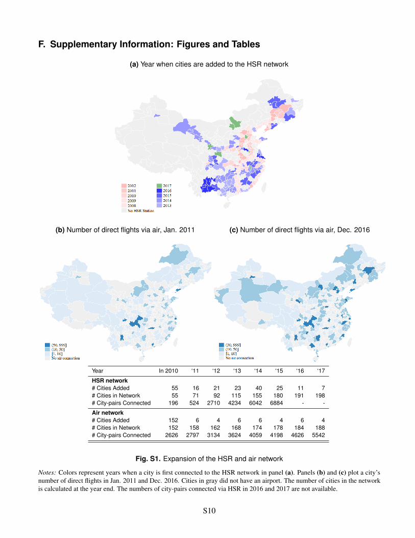
Figure S2 is analogous to Figure 1 and presents descriptive evidence on the benefit of improved transportationnetworks in mitigating households’ exposure to extreme temperature. The top panel of Figure S2 plots the temperaturelevel experienced by travelers against temperature levels at their home cities. The colored lines represent the localpolynomial smoothed averages of the raw data for city-days with HSR connections (blue) and city-days without HSR(red), respectively. The bottom panel presents the empirical temperature distribution for city-days with HSR (blue)and city-days without HSR (red).

Travelers with HSR connections experience warmer temperatures during cold seasons (temperature below 37◦F) athome and cooler temperatures during mild and hot seasons (temperature above 37◦F). These differences can reach5 degrees and are statistically significant throughout most of the distribution, except in the tails when estimatesare noisier.¶ The bottom panel shows that the home city’s temperature is slightly higher for city-days with HSRaccess. This is largely due to cross-sectional variation, as cities with HSR are more likely to be found in the warmersouth. Figure S2 complements Figure 1 in the main text and provides descriptive evidence on the benefit of improvedtransportation networks in mitigating households’ exposure to adverse environmental conditions.

Figure S4 further maps the geographical distribution of HSR’s impact in reducing pollution exposure across citiesduring each city’s 50 most polluted days between 2014 - 2016. The outcome variable is the difference in µg/m3

between the pollution level at the home city and travelers’ actual exposure. Hence the figure illustrates travelers’benefit of leaving their home city during their home city’s 50 most polluted days between 2014 - 2016. A largerpositive number denotes a higher benefit. Cities outlined by thick black borders were connected to the HSR networkby 2013. We use the most polluted days between 2014-2016 instead of 2013-2016 since some cities did not haveHSR connections during the winter of 2013 when several episodes of extreme pollution occurred.

Cities that experience larger reductions in travelers’ pollution exposure, on days of intense home exposure, areshown in darker green. It is evident from the map that cities with HSR connections are more likely to exhibit largerreductions relative to their neighbors without such connections. Cities that reap the greatest benefit in pollutionreduction tend to be located in Northern China, which has experienced the country’s worst pollution over the pastdecade, especially in winter months.

Figure S5 presents travelers’ benefits in terms of temperature exposure in each city’s 50 hottest (left panel) and50 coldest days (right panel) during 2014 - 2016. Travelers’ benefit is measured by the difference between theiractual exposure and the temperature at the home city. Darker green colors represent travelers experiencing coolertemperatures during hottest days (left panel) and warmer temperatures during coldest days (right panel). Cities inSoutheastern China with HSR access display the largest benefits during the hottest days, as the majority of these citiesfalls into the humid subtropical climate category and are vulnerable to heat waves. Similarly, cities in NortheasternChina with HSR access benefit more on the coldest days, when the temperature falls below zero. These trips arefacilitated by several north-south HSR lines that travel across a wide temperature range (e.g. the Beijing - Wuhanline). The contrast between cities on and off the HSR lines reflects the mitigating effect of HSR connections, exceptfor southeastern cities in cold days when these cities are much warmer than the rest of the country.

Table S2 illustrates travel patterns by destination cities’ temperature, analogous to Table 1. Since extremetemperature includes both cold and hot days, we divide the temperature distribution into ten bins (decile), five bins for

¶The standard errors are calculated using the Epanechnikov kernel and optimal bandwidth in STATA.

S3

temperatures below 61 ◦F (the median) and five bins for temperatures above 61 ◦F. Each row of the table reportsthe fraction of travelers visiting each of the ten temperature bins, conditioning on the decile of home temperature.The last two columns report the average temperature experienced by travelers and that at their home city. Panels(a) and (b) present the statistics for non-HSR travelers and HSR-travelers, respectively, and Panel (c) reports theirdifference. For example, when the home city’s temperature is in the coldest decile, travelers with HSR access are8.6 percentage points more likely to visit warmer destinations than travelers without HSR access. Similarly, whenthe home city’s temperature is in the highest decile, travelers with HSR access are 7.7 percentage points more likelyto visit cooler destinations than travelers without HSR access. Table S2 complements Table 1 in the main text andprovides additional descriptive evidence on the benefit of improved transportation networks.

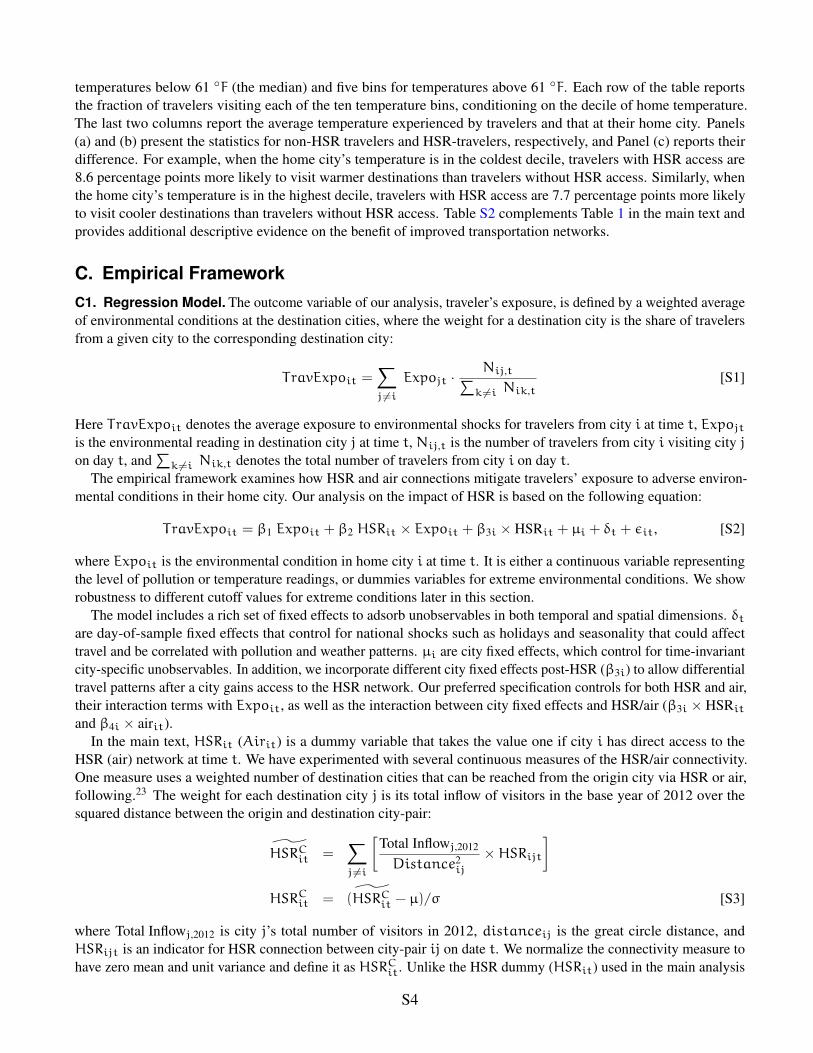
C. Empirical FrameworkC1. Regression Model. The outcome variable of our analysis, traveler’s exposure, is defined by a weighted averageof environmental conditions at the destination cities, where the weight for a destination city is the share of travelersfrom a given city to the corresponding destination city:

TravExpoit =∑j6=i

Expojt ·Nij,t∑

k6=i Nik,t[S1]

Here TravExpoit denotes the average exposure to environmental shocks for travelers from city i at time t, Expojtis the environmental reading in destination city j at time t, Nij,t is the number of travelers from city i visiting city jon day t, and

∑k6=i Nik,t denotes the total number of travelers from city i on day t.

The empirical framework examines how HSR and air connections mitigate travelers’ exposure to adverse environ-mental conditions in their home city. Our analysis on the impact of HSR is based on the following equation:

TravExpoit = β1 Expoit + β2 HSRit × Expoit + β3i × HSRit + µi + δt + εit, [S2]

where Expoit is the environmental condition in home city i at time t. It is either a continuous variable representingthe level of pollution or temperature readings, or dummies variables for extreme environmental conditions. We showrobustness to different cutoff values for extreme conditions later in this section.

The model includes a rich set of fixed effects to adsorb unobservables in both temporal and spatial dimensions. δtare day-of-sample fixed effects that control for national shocks such as holidays and seasonality that could affecttravel and be correlated with pollution and weather patterns. µi are city fixed effects, which control for time-invariantcity-specific unobservables. In addition, we incorporate different city fixed effects post-HSR (β3i) to allow differentialtravel patterns after a city gains access to the HSR network. Our preferred specification controls for both HSR and air,their interaction terms with Expoit, as well as the interaction between city fixed effects and HSR/air (β3i × HSRit

and β4i × airit).In the main text, HSRit (Airit) is a dummy variable that takes the value one if city i has direct access to the

HSR (air) network at time t. We have experimented with several continuous measures of the HSR/air connectivity.One measure uses a weighted number of destination cities that can be reached from the origin city via HSR or air,following.23 The weight for each destination city j is its total inflow of visitors in the base year of 2012 over thesquared distance between the origin and destination city-pair:

HSRCit =∑j6=i

[Total Inflowj,2012

Distance2ij

×HSRijt]

HSRCit = (HSRCit − µ)/σ [S3]

where Total Inflowj,2012 is city j’s total number of visitors in 2012, distanceij is the great circle distance, andHSRijt is an indicator for HSR connection between city-pair ij on date t. We normalize the connectivity measure tohave zero mean and unit variance and define it as HSRCit. Unlike the HSR dummy (HSRit) used in the main analysis

S4

whose value remains the same after a city is first connected to the HSR network, HSRCit increases whenever cityi is connected to additional destinations as the HSR network expands. In addition, this measure also depends oncities’ centrality in the transportation network. The connectivity measure for air (airCit) is defined analogously. Otherconnectivity measures include replacing distance squared with distance and/or removing the destination city’s inflow(Total Inflowj,2012) in the weights. Our results are robust to these different measures of connectivity.

Parameter β1 captures the relationship between a given home city’s environmental condition and its travelers’exposure. While both pollution and temperature are correlated geographically, the spatial correlation decays acrossspace. In the absence of a strong correlation between the trip direction and destination conditions (e.g., all trips goingfrom dirty to dirty cities), one should expect to see 0 < β1 < 1.

Parameter β2 measures how HSR access affects the relationship between home conditions and travelers’ exposure.If HSR facilitates residents’ ability to mitigate adverse environmental conditions at home, β2 should be negative. Theidentification of β2 is based on the standard difference-in-differences (DID) design. Taking pollution (PM2.5) as anexample, when Expoit is a dummy variable for local extreme pollution, the DID estimator of β2 measures HSR’simpact on travelers’ exposure during polluted days relative to its impact during clean days, while using cities withoutHSR as a control group. The key identification assumption is the standard common-trend assumption, where there areno confounding factors that affect the relationship between home city’s pollution level and traveler’s exposure beforeand after the HSR connection.

In principle, if HSR connection simply enables travelers to travel further to destinations whose pollution andtemperature are less correlated to those at home, the aggregate benefit in terms of pollution mitigation could beeither negative or positive. For example, travelers might visit dirty places when home cities are clean and such anegative effect could dominate the benefit from mitigation when the home city is polluted. Hence, whether improvedtransportation facilitates mitigation on net is an empirical question. Our measure of the aggregate benefit of improvedtransportation infrastructure is −

∑i,tωi,t(β2 ∗Expoit+β3i), whereωi,t is city-i-day-t’s share of travelers among

all cities with HSR access in our sample period. All regressions are weighted by the number of home city i’s travelersat time t, so that the effect sizes reported below can be interpreted as the national average across all travel.

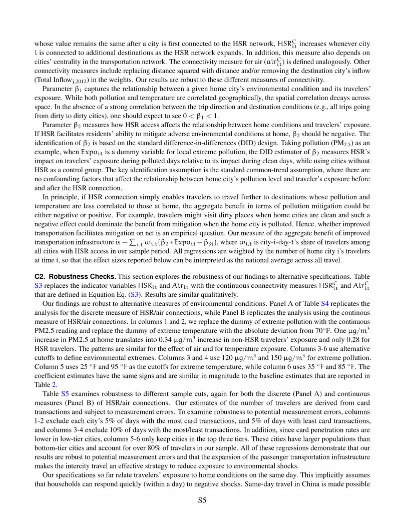
C2. Robustness Checks. This section explores the robustness of our findings to alternative specifications. TableS3 replaces the indicator variables HSRit and Airit with the continuous connectivity measures HSRCit and AirCitthat are defined in Equation Eq. (S3). Results are similar qualitatively.

Our findings are robust to alternative measures of environmental conditions. Panel A of Table S4 replicates theanalysis for the discrete measure of HSR/air connections, while Panel B replicates the analysis using the continousmeasure of HSR/air connections. In columns 1 and 2, we replace the dummy of extreme pollution with the continuousPM2.5 reading and replace the dummy of extreme temperature with the absolute deviation from 70◦F. One µg/m3

increase in PM2.5 at home translates into 0.34 µg/m3 increase in non-HSR travelers’ exposure and only 0.28 forHSR travelers. The patterns are similar for the effect of air and for temperature exposure. Columns 3-6 use alternativecutoffs to define environmental extremes. Columns 3 and 4 use 120 µg/m3 and 150 µg/m3 for extreme pollution.Column 5 uses 25 ◦F and 95 ◦F as the cutoffs for extreme temperature, while column 6 uses 35 ◦F and 85 ◦F. Thecoefficient estimates have the same signs and are similar in magnitude to the baseline estimates that are reported inTable 2.

Table S5 examines robustness to different sample cuts, again for both the discrete (Panel A) and continuousmeasures (Panel B) of HSR/air connections. Our estimates of the number of travelers are derived from cardtransactions and subject to measurement errors. To examine robustness to potential measurement errors, columns1-2 exclude each city’s 5% of days with the most card transactions, and 5% of days with least card transactions,and columns 3-4 exclude 10% of days with the most/least transactions. In addition, since card penetration rates arelower in low-tier cities, columns 5-6 only keep cities in the top three tiers. These cities have larger populations thanbottom-tier cities and account for over 80% of travelers in our sample. All of these regressions demonstrate that ourresults are robust to potential measurement errors and that the expansion of the passenger transportation infrastructuremakes the intercity travel an effective strategy to reduce exposure to environmental shocks.

Our specifications so far relate travelers’ exposure to home conditions on the same day. This implicitly assumesthat households can respond quickly (within a day) to negative shocks. Same-day travel in China is made possible

S5

by the expansive network and numerous train- and flight-departures that are scheduled daily for most cities. Ampleevidence cites households using pollution and weather forecasts to travel to desirable places in events of extremepollution and heat waves.14, 15, 16 As a result, “Haze-avoidance tourism” and “smog refugees” have become newthemes in intercity travel in recent years.

Nonetheless, to allow the possibility that households react with a lag to pollution and temperature shock (dueto the time constraint it takes to respond), or even in advance of such a shock (due to the wide availability andincreasing accuracy of forecasts), Table S6 replaces the daily environmental measure Expoit with its average leadsin the following week (column 1) and average lags in the previous week (column 2). Similar to Tables S3-S5,Panel A presents results for discrete HSR/air connections and panel B reports results using continuous measures ofconnections. Travelers respond to both leading and lagged home pollution/temperature, though the magnitudes aresmaller than responses to contemporary conditions. These results suggests that HSR/air facilitates adaptation to bothcontemporaneous environmental shocks and recent and future shocks.

C3. Extensive Margin. Up to now, our analysis has focused on the intensive margin of travel responses: the roleof HSR/air in assisting travelers from pollution-hit cities to access cleaner destinations. However, adjustments atthe extensive margin could also be relevant. It is unclear ex-ante whether people might be expected to travel morewhen pollution is worse in their home city. On the one hand, people might travel to cleaner cities as a means ofavoidance. On the other hand, people might reduce outdoor activities entirely, thus limiting their intercity travel.Table S7 evaluates such extensive margin responses by using the log number of travelers in a city-day.

Corroborating existing findings in the literature,38, 39, 40 we find that residents travel significantly less when theirhome cities are subject to extreme pollution. This is consistent with the observation that residents stay indoors toavoid exposure, as advocated by government and media. On the other hand, having access to HSR/air networksincreases the frequency of travel, especially for trips with a medium or long distance (longer than 300km or 500km).The coefficients are somewhat small and noisy, suggesting that the extensive margin is unlikely to be the primarychannel underlying the avoidance behavior documented above.

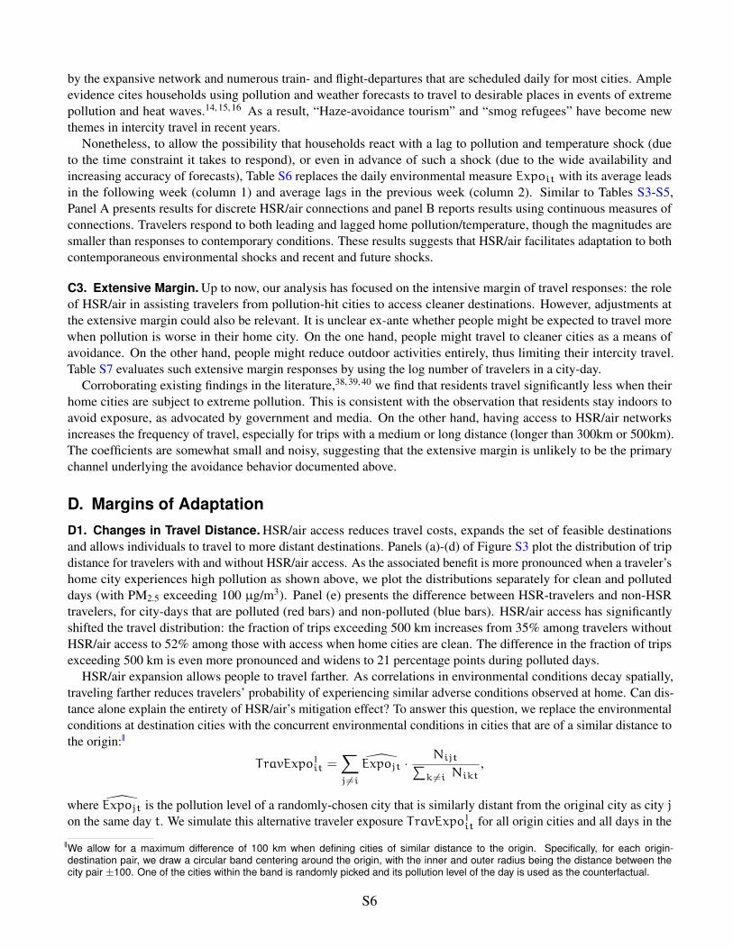
D. Margins of AdaptationD1. Changes in Travel Distance. HSR/air access reduces travel costs, expands the set of feasible destinationsand allows individuals to travel to more distant destinations. Panels (a)-(d) of Figure S3 plot the distribution of tripdistance for travelers with and without HSR/air access. As the associated benefit is more pronounced when a traveler’shome city experiences high pollution as shown above, we plot the distributions separately for clean and polluteddays (with PM2.5 exceeding 100 µg/m3). Panel (e) presents the difference between HSR-travelers and non-HSRtravelers, for city-days that are polluted (red bars) and non-polluted (blue bars). HSR/air access has significantlyshifted the travel distribution: the fraction of trips exceeding 500 km increases from 35% among travelers withoutHSR/air access to 52% among those with access when home cities are clean. The difference in the fraction of tripsexceeding 500 km is even more pronounced and widens to 21 percentage points during polluted days.

HSR/air expansion allows people to travel farther. As correlations in environmental conditions decay spatially,traveling farther reduces travelers’ probability of experiencing similar adverse conditions observed at home. Can dis-tance alone explain the entirety of HSR/air’s mitigation effect? To answer this question, we replace the environmentalconditions at destination cities with the concurrent environmental conditions in cities that are of a similar distance tothe origin:||

TravExpo1it =

∑j6=i

Expojt ·Nijt∑

k6=i Nikt,

where Expojt is the pollution level of a randomly-chosen city that is similarly distant from the original city as city jon the same day t. We simulate this alternative traveler exposure TravExpo1

it for all origin cities and all days in the

||We allow for a maximum difference of 100 km when defining cities of similar distance to the origin. Specifically, for each origin-destination pair, we draw a circular band centering around the origin, with the inner and outer radius being the distance between thecity pair ±100. One of the cities within the band is randomly picked and its pollution level of the day is used as the counterfactual.

S6

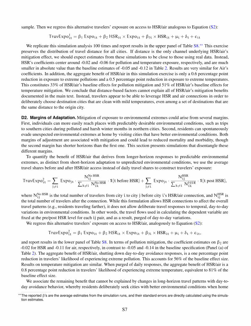
sample. Then we regress this alternative travelers’ exposure on access to HSR/air analogous to Equation (S2):

TravExpo1it = β1 Expoit + β2 HSRit × Expoit + β3i × HSRit + µi + δt + εit

We replicate this simulation analysis 100 times and report results in the upper panel of Table S8.** This exercisepreserves the distribution of travel distance for all cities. If distance is the only channel underlying HSR/air’smitigation effect, we should expect estimates from these simulations to be close to those using real data. Instead,HSR’s coefficients center around -0.02 and -0.06 for pollution and temperature exposure, respectively, and are muchsmaller in absolute value than the baseline estimates of -0.05 and -0.12 in Table 2. Results are very similar for Air’scoefficients. In addition, the aggregate benefit of HSR/air in this simulation exercise is only a 0.6 percentage pointreduction in exposure to extreme pollutions and a 0.5 percentage point reduction in exposure to extreme temperatures.This constitutes 33% of HSR/air’s baseline effects for pollution mitigation and 51% of HSR/air’s baseline effects fortemperature mitigation. We conclude that distance-based factors cannot explain all of HSR/air’s mitigation benefitsdocumented in the main text. Instead, travelers appear to be able to leverage HSR and air connections in order todeliberately choose destination cities that are clean with mild temperatures, even among a set of destinations that arethe same distance to the origin city.

D2. Margins of Adaptation. Mitigation of exposure to environmental extremes could arise from several margins.First, individuals can more easily reach places with predictably desirable environmental conditions, such as tripsto southern cities during polluted and harsh winter months in northern cities. Second, residents can spontaneouslyevade unexpected environmental extremes at home by visiting cities that have better environmental conditions. Bothmargins of adjustment are associated with mitigation and could lead to reduced mortality and morbidity, thoughthe second margin has shorter horizons than the first one. This section presents simulations that disentangle thesedifferent margins.

To quantify the benefit of HSR/air that derives from longer-horizon responses to predictable environmentalextremes, as distinct from short-horizon adaptation to unpredicted environmental conditions, we use the averagetravel shares before and after HSR/air access instead of daily travel shares to construct travelers’ exposure:

TravExpo2it =

∑j6=i

Expojt ·NNo HSR

ij∑k6=i N

No HSRik

· 1{t before HSR}+∑j6=i

Expojt ·NHSR

ij∑k6=i N

HSRik

· 1{t post HSR},

where NNo HSRij is the total number of travelers from city i to city j before city i’s HSR/air connection, and NHSR

ij isthe total number of travelers after the connection. While this formulation allows HSR connections to affect the overalltravel patterns (e.g., residents traveling farther), it does not allow deliberate travel responses to temporal, day-to-dayvariations in environmental conditions. In other words, the travel flows used in calculating the dependent variable arefixed at the pre/post HSR level for each ij pair, and as a result, purged of day-to-day variations.

We regress this alternative travelers’ exposure on access to HSR/air, analogously to Equation (S2):

TravExpo2it = β1 Expoit + β2 HSRit × Expoit + β3i × HSRit + µi + δt + εit,

and report results in the lower panel of Table S8. In terms of pollution mitigation, the coefficient estimates on β2 are-0.02 for HSR and -0.11 for air, respectively, in contrast to -0.05 and -0.14 in the baseline specification (Panel (a) ofTable 2). The aggregate benefit of HSR/air, shutting down day-to-day avoidance responses, is a one percentage pointreduction in travelers’ likelihood of experiencing extreme pollution. This accounts for 56% of the baseline effect size.Results on temperature mitigation are similar. When purged of daily responses, the aggregate benefit of HSR/air is a0.8 percentage point reduction in travelers’ likelihood of experiencing extreme temperature, equivalent to 81% of thebaseline effect size.

We associate the remaining benefit that cannot be explained by changes in long-horizon travel patterns with day-to-day avoidance behavior, whereby residents deliberately seek cities with better environmental conditions when home

**The reported β’s are the average estimates from the simulation runs, and their standard errors are directly calculated using the simula-tion estimates.

S7

city is hit by environmental extremes. For pollution mitigation, both the long-horizon and short-horizon adaptationsmatter, with the former and latter margins accounting for 56% and 44% of the aggregate benefit, respectively. Fortemperature exposure, day-to-day mitigation is less important and only explains 19% of the aggregate effect. This isbecause temperature extremes exhibit less geographical variation and hence are harder to escape from.

E. Mortality Benefits of Reduced ExposureAccording to the estimates in Column (1), Table S4, improved transportation infrastructure leads to a reduction of 9.1µg/m3 units in terms of exposure to PM2.5 for an average traveler on traveling days. This is equivalent to a 14%reduction in an average traveler’s pollution exposure. Using 2.5 days as the average trip duration calculated from theUnionPay dataset, the benefit translates to 0.062 µg/m3 unit reduction in travelers’ annual average PM2.5 exposure.

One µg/m3 unit increase in average PM10 exposure is estimated to reduce life expectancy by 0.064 years.17 Thepollution monitoring data in China suggest that one µg/m3 increase in PM2.5 corresponds to 1.5 µg/m3 increase inPM10. Hence, we consider the health consequence per-unit of PM2.5 exposure equivalent to 1.5 times that of PM10. In2016, 1.4 billion passengers traveled via HSR and 0.5 billion passengers traveled via airlines in China††.42, 43 Ourestimate therefore implies that the annual reduction in pollution exposure induced by improved HSR/air transportationnetworks translates into a potential savings of 5.7 million life-years in 2016.

For the mortality impact of temperature extreme, we follow the age-specific dose-response functions fromDeschênes et al.44 Based on the age structure of China’s population, their estimates suggest that an increase ofone-day exposure to temperature extremes will raise the mortality rate by 5 to 10 per million population.‡‡ Ourestimates from Table S4 show that the improved transportation network reduces an average traveler’s exposure totemperature extremes by 3.28 days per year. Taken together, these estimates suggest that mitigation in exposure totemperature extremes as a result of the HSR/air expansion leads to 143 to 268 thousand lives saved each year.

24. Y. Dian-Xiu, Y. Ji-Fu, C. Zheng-Hong, Z. You-Fei, W. Rong-Jun, Spatial and temporal variations of heat waves in China from 1961 to2010, Advances in Climate Change Research 5, 66 (2014).

25. M. Luo, N.-C. Lau, Heat waves in southern China: Synoptic behavior, long-term change, and urbanization effects, Journal of Climate30, 703 (2017).

26. C. Behrens, E. Pels, Intermodal competition in the London–Paris passenger market: High-Speed Rail and air transport, Journal ofUrban Economics 71, 278 (2012).

27. A. B. Bernard, A. Moxnes, Y. U. Saito, Production networks, geography, and firm performance, Journal of Political Economy 127, 000(2019).

28. D. Donaldson, Railroads of the Raj: Estimating the impact of transportation infrastructure, American Economic Review 108, 899(2018).

29. S. Zheng, M. E. Kahn, China’s bullet trains facilitate market integration and mitigate the cost of megacity growth, Proceedings of theNational Academy of Sciences 110, E1248 (2013).

30. B. Faber, Trade integration, market size, and industrialization: evidence from China’s National Trunk Highway System, Review ofEconomic Studies 81, 1046 (2014).

31. Y. Lin, Travel costs and urban specialization patterns: Evidence from China’s high speed railway system, Journal of Urban Economics98, 98 (2017).

32. N. Baum-Snow, Changes in transportation infrastructure and commuting patterns in US metropolitan areas, 1960-2000, AmericanEconomic Review 100, 378 (2010).

33. D. Donaldson, R. Hornbeck, Railroads and American economic growth: A market access approach, The Quarterly Journal of Eco-nomics 131, 799 (2016).

34. X. Dong, S. Zheng, M. E. Kahn, The Role of Transportation Speed in Facilitating High Skilled Teamwork, Journal of Urban Economics(2020).

35. A. Agrawal, A. Galasso, A. Oettl, Roads and innovation, Review of Economics and Statistics 99, 417 (2017).36. R. Burgess, D. Donaldson, Can openness mitigate the effects of weather shocks? Evidence from India’s famine era, American Economic

Review 100, 449 (2010).37. M. E. Kahn, S. Zheng, Blue skies over Beijing: Economic growth and the environment in China (Princeton University Press, 2016).38. E. Moretti, M. Neidell, Pollution, Health, and Avoidance Behavior: Evidence from the Ports of Los Angeles, Journal of Human Resources

46, 154 (2011).39. J. Zivin, M. Kotchen, E. Mansur, Spatial and Temporal Heterogeneity of Marginal Emissions: Implications for Electric Cars and Other

Electricity-Shifting Policies, Journal of Economic Behavior and Organization 107, 248 (2014).40. P. J. Barwick, S. Li, D. Rao, N. B. Zahur, The morbidity cost of air pollution: evidence from consumer spending in China (2018).

††We assume all trips are round trips, thus the number of travelers being half of the total ridership.‡‡Specifically, for an increase of one-day exposure to temperature extremes on the population, the mortality rate will increase from 5629.6

per year per million people to 5634.2-5638.2 deaths per year per million people.

S8

41. A. Ebenstein, M. Fan, M. Greenstone, G. He, M. Zhou, New evidence on the impact of sustained exposure to air pollution on lifeexpectancy from China’s Huai River Policy, Proceedings of the National Academy of Sciences 114, 10384 (2017).

42. Xinhua, 1.4 Billion Passengers Rode China’s HSR Last Year, Renmin Ribao (2017).43. CAAC, Statistics on China’s Civil Aviation Industry Development (2017).44. O. Deschenes, M. Greenstone, Climate Change, Mortality, and Adaptation: Evidence from Annual Fluctuations in Weather in the US,

American Economic Journal: Applied Economics 3, 152 (2011).

S9

F. Supplementary Information: Figures and Tables

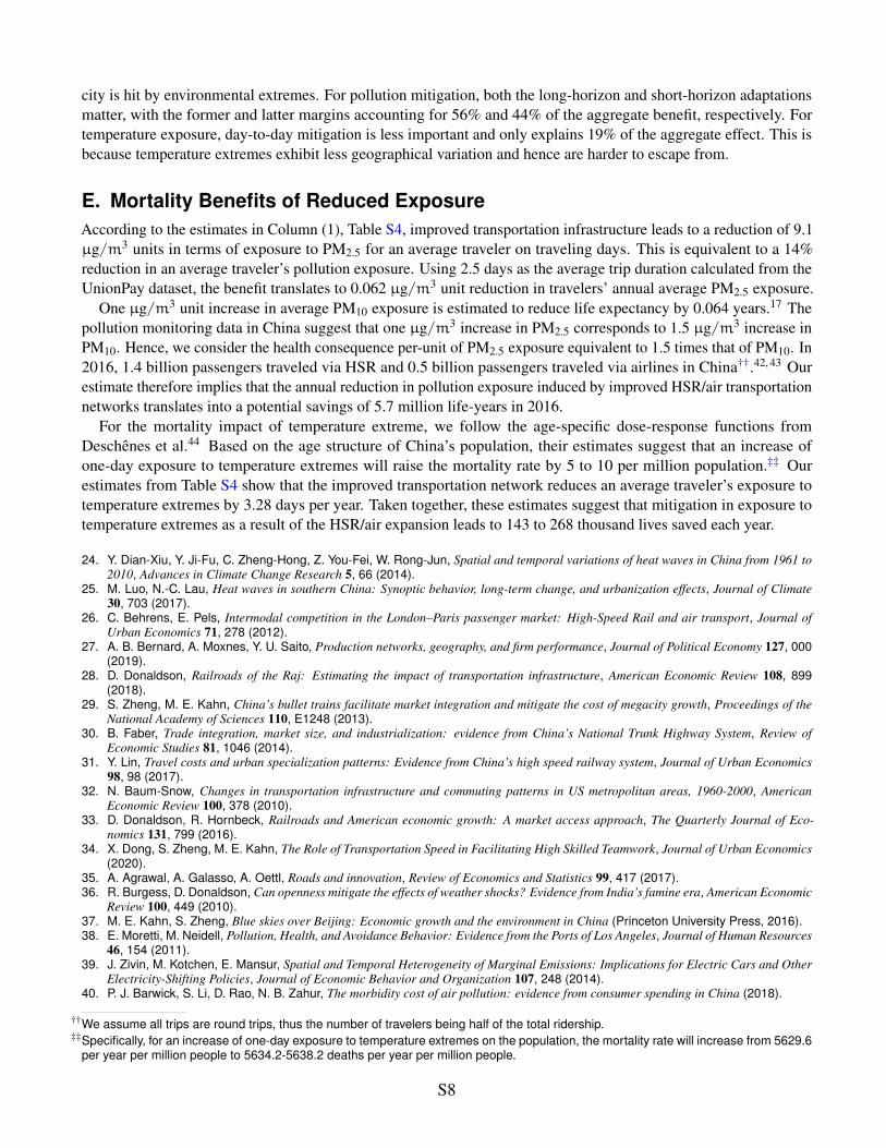
(a) Year when cities are added to the HSR network

(b) Number of direct flights via air, Jan. 2011 (c) Number of direct flights via air, Dec. 2016

Year In 2010 ‘11 ‘12 ‘13 ‘14 ‘15 ‘16 ‘17

HSR network# Cities Added 55 16 21 23 40 25 11 7# Cities in Network 55 71 92 115 155 180 191 198# City-pairs Connected 196 524 2710 4234 6042 6884 - -

Air network# Cities Added 152 6 4 6 6 4 6 4# Cities in Network 152 158 162 168 174 178 184 188# City-pairs Connected 2626 2797 3134 3624 4059 4198 4626 5542

Fig. S1. Expansion of the HSR and air network

Notes: Colors represent years when a city is first connected to the HSR network in panel (a). Panels (b) and (c) plot a city’snumber of direct flights in Jan. 2011 and Dec. 2016. Cities in gray did not have an airport. The number of cities in the networkis calculated at the year end. The numbers of city-pairs connected via HSR in 2016 and 2017 are not available.

S10

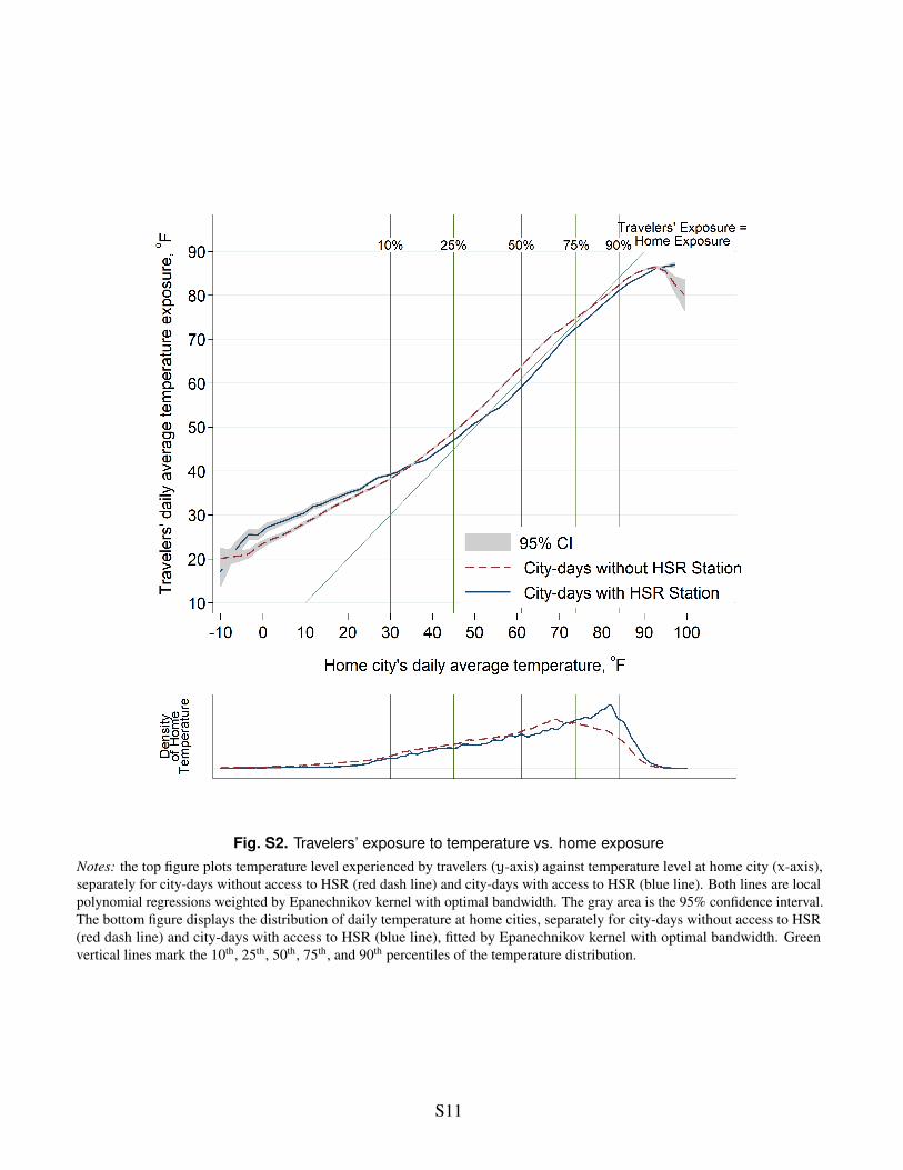
Fig. S2. Travelers’ exposure to temperature vs. home exposureNotes: the top figure plots temperature level experienced by travelers (y-axis) against temperature level at home city (x-axis),separately for city-days without access to HSR (red dash line) and city-days with access to HSR (blue line). Both lines are localpolynomial regressions weighted by Epanechnikov kernel with optimal bandwidth. The gray area is the 95% confidence interval.The bottom figure displays the distribution of daily temperature at home cities, separately for city-days without access to HSR(red dash line) and city-days with access to HSR (blue line), fitted by Epanechnikov kernel with optimal bandwidth. Greenvertical lines mark the 10th, 25th, 50th, 75th, and 90th percentiles of the temperature distribution.

S11

(a) Trip distances for cities without HSR/air ac-cess during clean days

(b) Trip distances for cities with HSR/air ac-cess during clean days

(c) Trip distances for cities without HSR/air ac-cess during polluted days

(d) Trip distances for cities with HSR/air ac-cess during polluted days

(e) Difference in trip distances

Fig. S3. Trip distance for city-days w. and w/o HSR/air during clean and polluted days

Notes: panels (a)-(d): histograms for trip distances for cities without or with HSR/air access during clean and polluted(PM2.5 > 100µg/m3) days. Panel (e) plots differences in traveler density between cities with HSR/air access and cities without,on polluted days (red bars) and clean days (blue bars). Travelers from cities with HSR/air access are more likely to visit distantdestinations and especially so when home cities experience extreme pollution.

S12

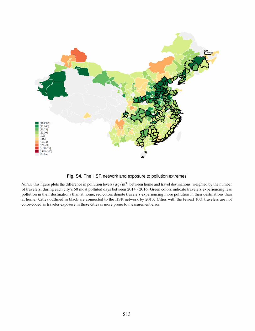
Fig. S4. The HSR network and exposure to pollution extremes

Notes: this figure plots the difference in pollution levels (µg/m3) between home and travel destinations, weighted by the numberof travelers, during each city’s 50 most polluted days between 2014 - 2016. Green colors indicate travelers experiencing lesspollution in their destinations than at home; red colors denote travelers experiencing more pollution in their destinations thanat home. Cities outlined in black are connected to the HSR network by 2013. Cities with the fewest 10% travelers are notcolor-coded as traveler exposure in these cities is more prone to measurement error.

S13

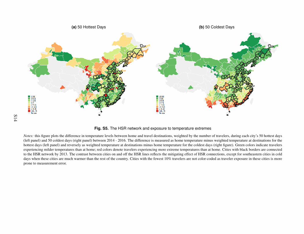
(a) 50 Hottest Days (b) 50 Coldest Days

Fig. S5. The HSR network and exposure to temperature extremes

Notes: this figure plots the difference in temperature levels between home and travel destinations, weighted by the number of travelers, during each city’s 50 hottest days(left panel) and 50 coldest days (right panel) between 2014 - 2016. The difference is measured as home temperature minus weighted temperature at destinations for thehottest days (left panel) and reversely as weighted temperature at destinations minus home temperature for the coldest days (right figure). Green colors indicate travelersexperiencing milder temperatures than at home; red colors denote travelers experiencing more extreme temperatures than at home. Cities with black borders are connectedto the HSR network by 2013. The contrast between cities on and off the HSR lines reflects the mitigating effect of HSR connections, except for southeastern cities in colddays when these cities are much warmer than the rest of the country. Cities with the fewest 10% travelers are not color-coded as traveler exposure in these cities is moreprone to measurement error.

S14

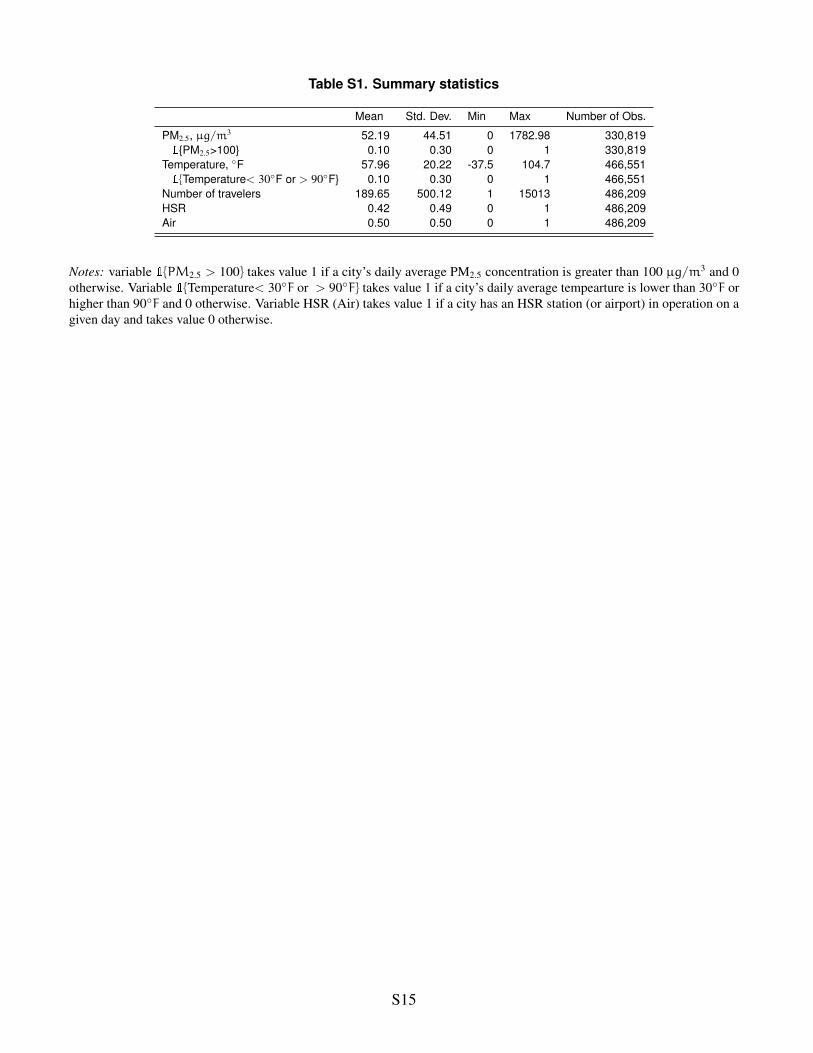
Table S1. Summary statistics

Mean Std. Dev. Min Max Number of Obs.

PM2.5, µg/m3 52.19 44.51 0 1782.98 330,8191{PM2.5>100} 0.10 0.30 0 1 330,819

Temperature, ◦F 57.96 20.22 -37.5 104.7 466,5511{Temperature< 30◦F or > 90◦F} 0.10 0.30 0 1 466,551

Number of travelers 189.65 500.12 1 15013 486,209HSR 0.42 0.49 0 1 486,209Air 0.50 0.50 0 1 486,209

Notes: variable 1{PM2.5 > 100} takes value 1 if a city’s daily average PM2.5 concentration is greater than 100 µg/m3 and 0otherwise. Variable 1{Temperature< 30◦F or > 90◦F} takes value 1 if a city’s daily average tempearture is lower than 30◦F orhigher than 90◦F and 0 otherwise. Variable HSR (Air) takes value 1 if a city has an HSR station (or airport) in operation on agiven day and takes value 0 otherwise.

S15

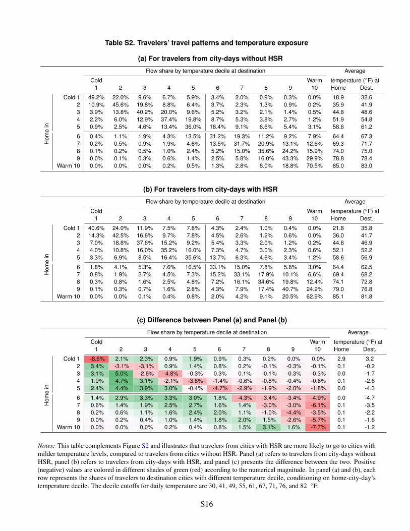
Table S2. Travelers’ travel patterns and temperature exposure

(a) For travelers from city-days without HSR

Flow share by temperature decile at destination Average

Cold Warm temperature (◦F) at1 2 3 4 5 6 7 8 9 10 Home Dest.

Hom

ein

Cold 1 49.2% 22.0% 9.6% 6.7% 5.9% 3.4% 2.0% 0.9% 0.3% 0.0% 18.9 32.62 10.9% 45.6% 19.8% 8.8% 6.4% 3.7% 2.3% 1.3% 0.9% 0.2% 35.9 41.93 3.9% 13.8% 40.2% 20.0% 9.6% 5.2% 3.2% 2.1% 1.4% 0.5% 44.8 48.64 2.2% 6.0% 12.9% 37.4% 19.8% 8.7% 5.3% 3.8% 2.7% 1.2% 51.9 54.85 0.9% 2.5% 4.6% 13.4% 36.0% 18.4% 9.1% 6.6% 5.4% 3.1% 58.6 61.2

6 0.4% 1.1% 1.9% 4.3% 13.5% 31.2% 19.3% 11.2% 9.2% 7.9% 64.4 67.37 0.2% 0.5% 0.9% 1.9% 4.6% 13.5% 31.7% 20.9% 13.1% 12.6% 69.3 71.78 0.1% 0.2% 0.5% 1.0% 2.4% 5.2% 15.0% 35.6% 24.2% 15.9% 74.0 75.09 0.0% 0.1% 0.3% 0.6% 1.4% 2.5% 5.8% 16.0% 43.3% 29.9% 78.8 78.4

Warm 10 0.0% 0.0% 0.0% 0.2% 0.5% 1.3% 2.8% 6.0% 18.8% 70.5% 85.0 83.0

(b) For travelers from city-days with HSR

Flow share by temperature decile at destination Average

Cold Warm temperature (◦F) at1 2 3 4 5 6 7 8 9 10 Home Dest.

Hom

ein

Cold 1 40.6% 24.0% 11.9% 7.5% 7.8% 4.3% 2.4% 1.0% 0.4% 0.0% 21.8 35.82 14.3% 42.5% 16.6% 9.7% 7.8% 4.5% 2.6% 1.2% 0.6% 0.0% 36.0 41.73 7.0% 18.8% 37.6% 15.2% 9.2% 5.4% 3.3% 2.0% 1.2% 0.2% 44.8 46.94 4.0% 10.8% 16.0% 35.2% 16.0% 7.3% 4.7% 3.0% 2.3% 0.6% 52.1 52.25 3.3% 6.9% 8.5% 16.4% 35.6% 13.7% 6.3% 4.6% 3.4% 1.2% 58.6 56.9

6 1.8% 4.1% 5.3% 7.6% 16.5% 33.1% 15.0% 7.8% 5.8% 3.0% 64.4 62.57 0.8% 1.9% 2.7% 4.5% 7.3% 15.2% 33.1% 17.9% 10.1% 6.6% 69.4 68.28 0.3% 0.8% 1.6% 2.5% 4.8% 7.2% 16.1% 34.6% 19.8% 12.4% 74.1 72.89 0.1% 0.3% 0.7% 1.6% 2.8% 4.3% 7.9% 17.4% 40.7% 24.2% 79.0 76.8

Warm 10 0.0% 0.0% 0.1% 0.4% 0.8% 2.0% 4.2% 9.1% 20.5% 62.9% 85.1 81.8

(c) Difference between Panel (a) and Panel (b)

Flow share by temperature decile at destination Average

Cold Warm temperature (◦F) at1 2 3 4 5 6 7 8 9 10 Home Dest.

Hom

ein

Cold 1 -8.6% 2.1% 2.3% 0.9% 1.9% 0.9% 0.3% 0.2% 0.0% 0.0% 2.9 3.22 3.4% -3.1% -3.1% 0.9% 1.4% 0.8% 0.2% -0.1% -0.3% -0.1% 0.1 -0.23 3.1% 5.0% -2.6% -4.8% -0.3% 0.3% 0.1% -0.1% -0.3% -0.3% 0.0 -1.74 1.9% 4.7% 3.1% -2.1% -3.8% -1.4% -0.6% -0.8% -0.4% -0.6% 0.1 -2.65 2.4% 4.4% 3.9% 3.0% -0.4% -4.7% -2.9% -1.9% -2.0% -1.8% 0.0 -4.3

6 1.4% 2.9% 3.3% 3.3% 3.0% 1.8% -4.3% -3.4% -3.4% -4.9% 0.0 -4.77 0.6% 1.4% 1.9% 2.5% 2.7% 1.6% 1.4% -3.0% -3.0% -6.1% 0.1 -3.58 0.2% 0.6% 1.1% 1.6% 2.4% 2.0% 1.1% -1.0% -4.4% -3.5% 0.1 -2.29 0.0% 0.2% 0.4% 1.0% 1.4% 1.8% 2.0% 1.5% -2.6% -5.7% 0.1 -1.6

Warm 10 0.0% 0.0% 0.0% 0.2% 0.4% 0.8% 1.5% 3.1% 1.6% -7.7% 0.1 -1.2

Notes: This table complements Figure S2 and illustrates that travelers from cities with HSR are more likely to go to cities withmilder temperature levels, compared to travelers from cities without HSR. Panel (a) refers to travelers from city-days withoutHSR, panel (b) refers to travelers from city-days with HSR, and panel (c) presents the difference between the two. Positive(negative) values are colored in different shades of green (red) according to the numerical magnitude. In panel (a) and (b), eachrow represents the shares of travelers to destination cities with different temperature decile, conditioning on home-city-day’stemperature decile. The decile cutoffs for daily temperature are 30, 41, 49, 55, 61, 67, 71, 76, and 82 ◦F.

S16

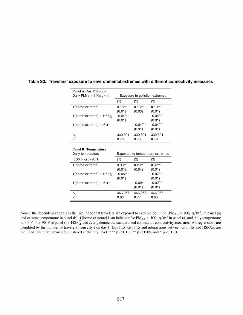
Table S3. Travelers’ exposure to environmental extremes with different connectivity measures

Panel A: Air PollutionDaily PM2.5 > 100µg/m3 Exposure to pollution extremes

(1) (2) (3)

1{home extreme} 0.18*** 0.13*** 0.19***(0.01) (0.03) (0.01)

1{home extreme}×HSRCit -0.04*** -0.04***

(0.01) (0.01)1{home extreme}×AirCit -0.04*** -0.04***

(0.01) (0.01)

N 330,801 330,801 330,801R2 0.78 0.78 0.79

Panel B: TemperatureDaily temperature Exposure to temperature extremes

< 30◦F or > 90◦F (1) (2) (3)

1{home extreme} 0.30*** 0.23*** 0.32***(0.01) (0.04) (0.01)

1{home extreme}×HSRCit -0.06*** -0.07***

(0.01) (0.01)1{home extreme}×AirCit -0.004 -0.02***

(0.01) (0.01)

N 466,257 466,257 466,257R2 0.80 0.77 0.80

Notes: the dependent variable is the likelihood that travelers are exposed to extreme pollution (PM2.5 > 100µg/m3) in panel (a)and extreme temperature in panel (b). 1{home extreme} is an indicator for PM2.5 > 100µg/m3 in panel (a) and daily temperature< 30◦F or > 90◦F in panel (b). HSRCit and AirCit denote the standardized continuous connectivity measures. All regressions areweighted by the number of travelers from city i on day t. Day FEs, city FEs and interactions between city FEs and HSR/air areincluded. Standard errors are clustered at the city level. *** p < 0.01, ** p < 0.05, and * p < 0.10.

S17

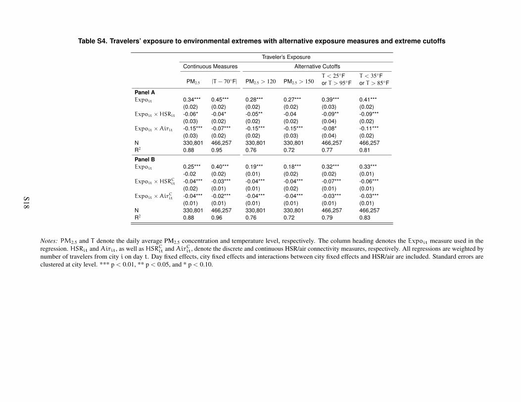
Table S4. Travelers’ exposure to environmental extremes with alternative exposure measures and extreme cutoffs

Traveler’s Exposure

Continuous Measures Alternative Cutoffs

PM2.5 |T − 70◦F| PM2.5 > 120 PM2.5 > 150T < 25◦F T < 35◦For T > 95◦F or T > 85◦F

Panel AExpoit 0.34*** 0.45*** 0.28*** 0.27*** 0.39*** 0.41***

(0.02) (0.02) (0.02) (0.02) (0.03) (0.02)Expoit ×HSRit -0.06* -0.04* -0.05** -0.04 -0.09** -0.09***

(0.03) (0.02) (0.02) (0.02) (0.04) (0.02)Expoit ×Airit -0.15*** -0.07*** -0.15*** -0.15*** -0.08* -0.11***

(0.03) (0.02) (0.02) (0.03) (0.04) (0.02)N 330,801 466,257 330,801 330,801 466,257 466,257R2 0.88 0.95 0.76 0.72 0.77 0.81

Panel BExpoit 0.25*** 0.40*** 0.19*** 0.18*** 0.32*** 0.33***

-0.02 (0.02) (0.01) (0.02) (0.02) (0.01)Expoit ×HSRC

it -0.04*** -0.03*** -0.04*** -0.04*** -0.07*** -0.06***(0.02) (0.01) (0.01) (0.02) (0.01) (0.01)

Expoit ×AirCit -0.04*** -0.02*** -0.04*** -0.04*** -0.03*** -0.03***(0.01) (0.01) (0.01) (0.01) (0.01) (0.01)

N 330,801 466,257 330,801 330,801 466,257 466,257R2 0.88 0.96 0.76 0.72 0.79 0.83

Notes: PM2.5 and T denote the daily average PM2.5 concentration and temperature level, respectively. The column heading denotes the Expoit measure used in theregression. HSRit and Airit, as well as HSRCit and AirCit, denote the discrete and continuous HSR/air connectivity measures, respectively. All regressions are weighted bynumber of travelers from city i on day t. Day fixed effects, city fixed effects and interactions between city fixed effects and HSR/air are included. Standard errors areclustered at city level. *** p < 0.01, ** p < 0.05, and * p < 0.10.

S18

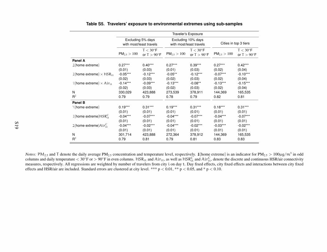
Table S5. Travelers’ exposure to environmental extremes using sub-samples

Traveler’s Exposure

Excluding 5% days Excluding 10% daysCities in top 3 tierswith most/least travels with most/least travels

PM2.5 > 100T < 30◦F

PM2.5 > 100T < 30◦F

PM2.5 > 100T < 30◦F

or T > 90◦F or T > 90◦F or T > 90◦F

Panel A1{home extreme} 0.27*** 0.40*** 0.27*** 0.39*** 0.27*** 0.42***

(0.01) (0.03) (0.01) (0.03) (0.02) (0.04)1{home extreme}×HSRit -0.05*** -0.12*** -0.05** -0.12*** -0.07*** -0.10***

(0.02) (0.03) (0.02) (0.03) (0.02) (0.04)1{home extreme}×Airit -0.14*** -0.09*** -0.13*** -0.08** -0.13*** -0.15***

(0.02) (0.03) (0.02) (0.03) (0.02) (0.04)N 330,029 423,888 273,539 378,911 144,369 165,535R2 0.79 0.79 0.78 0.79 0.82 0.81

Panel B1{home extreme} 0.19*** 0.31*** 0.19*** 0.31*** 0.18*** 0.31***

(0.01) (0.01) (0.01) (0.01) (0.01) (0.01)1{home extreme}HSRC

it -0.04*** -0.07*** -0.04*** -0.07*** -0.04*** -0.07***(0.01) (0.01) (0.01) (0.01) (0.01) (0.01)

1{home extreme}AirCit -0.04*** -0.02*** -0.04*** -0.02*** -0.03*** -0.02***(0.01) (0.01) (0.01) (0.01) (0.01) (0.01)

N 301,714 423,888 272,364 378,912 144,369 165,535R2 0.79 0.81 0.79 0.81 0.83 0.83

Notes: PM2.5 and T denote the daily average PM2.5 concentration and temperature level, respectively. 1{home extreme} is an indicator for PM2.5 > 100µg/m3 in oddcolumns and daily temperature < 30◦F or > 90◦F in even columns. HSRit and Airit, as well as HSRCit and AirCit, denote the discrete and continuous HSR/air connectivitymeasures, respectively. All regressions are weighted by number of travelers from city i on day t. Day fixed effects, city fixed effects and interactions between city fixedeffects and HSR/air are included. Standard errors are clustered at city level. *** p < 0.01, ** p < 0.05, and * p < 0.10.

S19

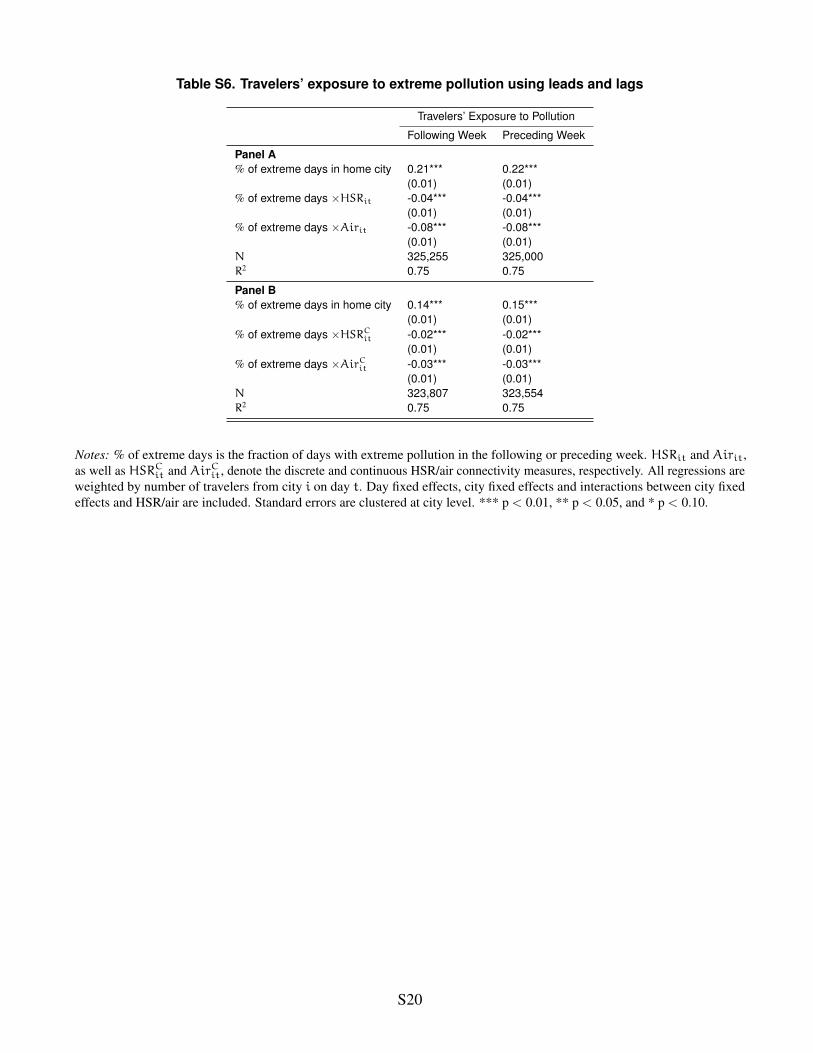
Table S6. Travelers’ exposure to extreme pollution using leads and lags

Travelers’ Exposure to Pollution

Following Week Preceding Week

Panel A% of extreme days in home city 0.21*** 0.22***

(0.01) (0.01)% of extreme days ×HSRit -0.04*** -0.04***

(0.01) (0.01)% of extreme days ×Airit -0.08*** -0.08***

(0.01) (0.01)N 325,255 325,000R2 0.75 0.75

Panel B% of extreme days in home city 0.14*** 0.15***

(0.01) (0.01)% of extreme days ×HSRC

it -0.02*** -0.02***(0.01) (0.01)

% of extreme days ×AirCit -0.03*** -0.03***(0.01) (0.01)

N 323,807 323,554R2 0.75 0.75

Notes: % of extreme days is the fraction of days with extreme pollution in the following or preceding week. HSRit and Airit,as well as HSRCit and AirCit, denote the discrete and continuous HSR/air connectivity measures, respectively. All regressions areweighted by number of travelers from city i on day t. Day fixed effects, city fixed effects and interactions between city fixedeffects and HSR/air are included. Standard errors are clustered at city level. *** p < 0.01, ** p < 0.05, and * p < 0.10.

S20

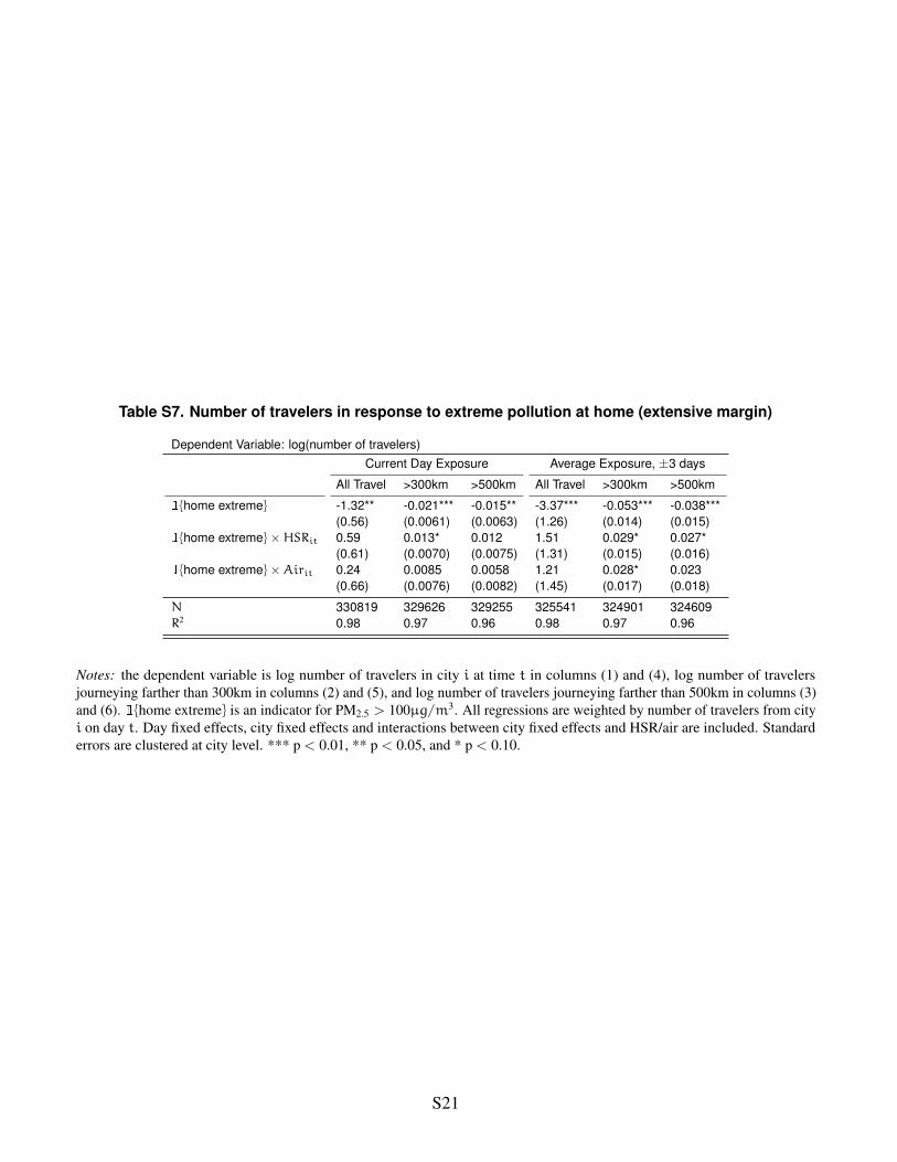
Table S7. Number of travelers in response to extreme pollution at home (extensive margin)

Dependent Variable: log(number of travelers)Current Day Exposure Average Exposure, ±3 days

All Travel >300km >500km All Travel >300km >500km

1{home extreme} -1.32** -0.021*** -0.015** -3.37*** -0.053*** -0.038***(0.56) (0.0061) (0.0063) (1.26) (0.014) (0.015)

1{home extreme}×HSRit 0.59 0.013* 0.012 1.51 0.029* 0.027*(0.61) (0.0070) (0.0075) (1.31) (0.015) (0.016)

1{home extreme}×Airit 0.24 0.0085 0.0058 1.21 0.028* 0.023(0.66) (0.0076) (0.0082) (1.45) (0.017) (0.018)

N 330819 329626 329255 325541 324901 324609R2 0.98 0.97 0.96 0.98 0.97 0.96

Notes: the dependent variable is log number of travelers in city i at time t in columns (1) and (4), log number of travelersjourneying farther than 300km in columns (2) and (5), and log number of travelers journeying farther than 500km in columns (3)and (6). 1{home extreme} is an indicator for PM2.5 > 100µg/m3. All regressions are weighted by number of travelers from cityi on day t. Day fixed effects, city fixed effects and interactions between city fixed effects and HSR/air are included. Standarderrors are clustered at city level. *** p < 0.01, ** p < 0.05, and * p < 0.10.

S21

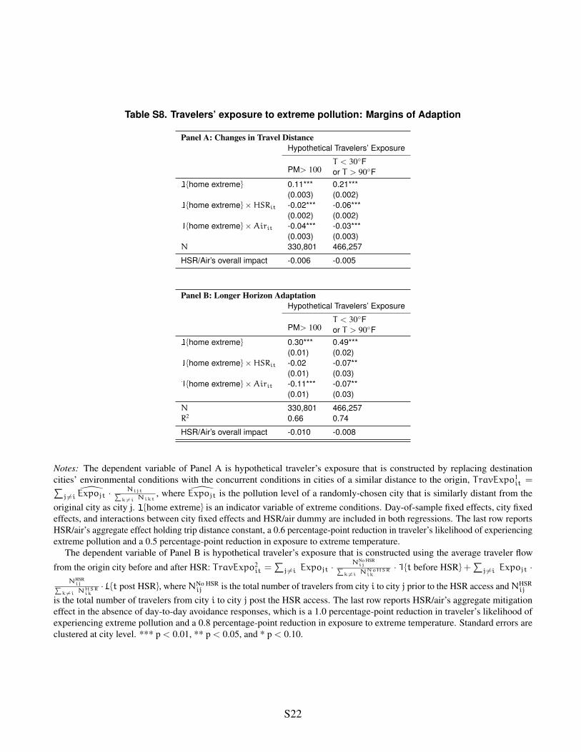
Table S8. Travelers’ exposure to extreme pollution: Margins of Adaption

Panel A: Changes in Travel DistanceHypothetical Travelers’ Exposure

PM> 100T < 30◦For T > 90◦F

1{home extreme} 0.11*** 0.21***(0.003) (0.002)

1{home extreme}×HSRit -0.02*** -0.06***(0.002) (0.002)

1{home extreme}×Airit -0.04*** -0.03***(0.003) (0.003)

N 330,801 466,257

HSR/Air’s overall impact -0.006 -0.005

Panel B: Longer Horizon AdaptationHypothetical Travelers’ Exposure

PM> 100T < 30◦For T > 90◦F

1{home extreme} 0.30*** 0.49***(0.01) (0.02)

1{home extreme}×HSRit -0.02 -0.07**(0.01) (0.03)

1{home extreme}×Airit -0.11*** -0.07**(0.01) (0.03)

N 330,801 466,257R2 0.66 0.74

HSR/Air’s overall impact -0.010 -0.008

Notes: The dependent variable of Panel A is hypothetical traveler’s exposure that is constructed by replacing destinationcities’ environmental conditions with the concurrent conditions in cities of a similar distance to the origin, TravExpo1

it =∑j6=i Expojt ·

Nijt∑k 6=i Nikt

, where Expojt is the pollution level of a randomly-chosen city that is similarly distant from theoriginal city as city j. 1{home extreme} is an indicator variable of extreme conditions. Day-of-sample fixed effects, city fixedeffects, and interactions between city fixed effects and HSR/air dummy are included in both regressions. The last row reportsHSR/air’s aggregate effect holding trip distance constant, a 0.6 percentage-point reduction in traveler’s likelihood of experiencingextreme pollution and a 0.5 percentage-point reduction in exposure to extreme temperature.

The dependent variable of Panel B is hypothetical traveler’s exposure that is constructed using the average traveler flow

from the origin city before and after HSR: TravExpo2it =

∑j6=i Expojt ·

NNo HSRij∑

k 6=i NNoHSRik

· 1{t before HSR}+∑

j6=i Expojt ·NHSR

ij∑k 6=i NHSR

ik

·1{t post HSR}, whereNNo HSRij is the total number of travelers from city i to city j prior to the HSR access andNHSR

ij

is the total number of travelers from city i to city j post the HSR access. The last row reports HSR/air’s aggregate mitigationeffect in the absence of day-to-day avoidance responses, which is a 1.0 percentage-point reduction in traveler’s likelihood ofexperiencing extreme pollution and a 0.8 percentage-point reduction in exposure to extreme temperature. Standard errors areclustered at city level. *** p < 0.01, ** p < 0.05, and * p < 0.10.

S22