Embed Size (px)
Citation preview
HAL Id: hal-03081151https://hal.inria.fr/hal-03081151
Submitted on 18 Dec 2020
HAL is a multi-disciplinary open accessarchive for the deposit and dissemination of sci-entific research documents, whether they are pub-lished or not. The documents may come fromteaching and research institutions in France orabroad, or from public or private research centers.
L’archive ouverte pluridisciplinaire HAL, estdestinée au dépôt et à la diffusion de documentsscientifiques de niveau recherche, publiés ou non,émanant des établissements d’enseignement et derecherche français ou étrangers, des laboratoirespublics ou privés.
Improvement of the modal expansion of electromagneticfields through interpolation
Marc Duruflé, Alexandre Gras, Philippe Lalanne
To cite this version:Marc Duruflé, Alexandre Gras, Philippe Lalanne. Improvement of the modal expansion of electromag-netic fields through interpolation. [Research Report] RR-9382, INRIA Bordeaux - Sud-Ouest. 2020.hal-03081151
ISS
N02
49-6
399
ISR
NIN
RIA
/RR
--93
82--
FR+E
NG
RESEARCHREPORTN° 9382December 2020
Project-Team Magique-3D
Improvement of themodal expansion ofelectromagnetic fieldsthrough interpolationMarc Duruflé, Alexandre Gras, Philippe Lalanne

RESEARCH CENTREBORDEAUX – SUD-OUEST
200 avenue de la Vieille Tour33405 Talence Cedex
Improvement of the modal expansion ofelectromagnetic fields through interpolation
Marc Duruflé∗, Alexandre Gras∗†, Philippe Lalanne†
Project-Team Magique-3D
Research Report n° 9382 — December 2020 — 38 pages
Abstract: We consider optical structures where the dielectric permittivity is described as a ratio-nal function of the pulsation ω (Lorentz model). The electromagnetic fields can be computed on alarge number of frequencies by computing the eigenmodes of the optical device and reconstructingthe solution by expanding it on these eigenmodes. This modal expansion suffers from numerouslimitations that are detailed in this report. In order to overcome these limitations, an interpolationprocedure is proposed such that the direct computation of the electric field is needed only for asmall number of interpolation points. Numerical experiments in 2-D and 3-D exhibit the efficiencyof this approach.
Key-words: electromagnetic resonance, quasinormal mode, microcavity, nanoresonator, modalexpansion
∗ Bordeaux INP, INRIA Bordeaux Sud-Ouest, EPI Magique 3-D† LP2N, Institut d’Optique Graduate School, CNRS, Univ. Bordeaux
Amélioration du développement modal des champsélectromagnétiques par une méthode d’interpolation
Résumé : Nous considérons des structures optiques où la permittivité diélectrique est unefonction rationelle de ω (modèle de Lorentz). Les champs électromagnétiques peuvent être cal-culés pour un grand nombre de fréquences en calculant les modes propres du dispositif optique eten reconstruisant la solution en la développant sur ces modes. Ce développement modal souffrede nombreuses limitations qui sont détaillées dans ce rapport. Afin de dépasser ces limitations,une procédure d’interpolation est proposée de telle sorte que le champ électrique est calculé di-rectement pour un petit nombre de points d’interpolation. Des expériences numériques en 2-Det 3-D montrent l’efficacité de cette approche.
Mots-clés : résonance électromagnétique, mode quasi-normal, microcavité, nano-résonateur,décomposition modale
Modal expansion and Interpolation 3
Contents
1 Introduction 3
2 General setting 4
3 Limitations of the modal expansion 63.1 Influence of the source term . . . . . . . . . . . . . . . . . . . . . . . . . . . . . . 6
3.1.1 Gaussian source . . . . . . . . . . . . . . . . . . . . . . . . . . . . . . . . 63.1.2 Incident plane wave . . . . . . . . . . . . . . . . . . . . . . . . . . . . . . 9
3.2 Dispersive materials . . . . . . . . . . . . . . . . . . . . . . . . . . . . . . . . . . 133.2.1 Germanium disk . . . . . . . . . . . . . . . . . . . . . . . . . . . . . . . . 133.2.2 Germanium sphere . . . . . . . . . . . . . . . . . . . . . . . . . . . . . . . 16
3.3 Summary of limitations . . . . . . . . . . . . . . . . . . . . . . . . . . . . . . . . 17
4 Efficient Computation of eigenmodes 184.1 Dispersive PMLs . . . . . . . . . . . . . . . . . . . . . . . . . . . . . . . . . . . . 184.2 Non-dispersive PMLs . . . . . . . . . . . . . . . . . . . . . . . . . . . . . . . . . . 194.3 Comparison of solvers . . . . . . . . . . . . . . . . . . . . . . . . . . . . . . . . . 19
5 Interpolation procedure to reconstruct the field 215.1 2-D cavity . . . . . . . . . . . . . . . . . . . . . . . . . . . . . . . . . . . . . . . . 225.2 3-D dolmen . . . . . . . . . . . . . . . . . . . . . . . . . . . . . . . . . . . . . . . 27
6 Conclusion 30
A Efficiency of interpolation on other cases 32A.1 2-D cobra cavity . . . . . . . . . . . . . . . . . . . . . . . . . . . . . . . . . . . . 32A.2 3-D cobra cavity . . . . . . . . . . . . . . . . . . . . . . . . . . . . . . . . . . . . 33A.3 Silica square . . . . . . . . . . . . . . . . . . . . . . . . . . . . . . . . . . . . . . . 33A.4 Germanium disk . . . . . . . . . . . . . . . . . . . . . . . . . . . . . . . . . . . . 34A.5 Germanium sphere . . . . . . . . . . . . . . . . . . . . . . . . . . . . . . . . . . . 36
B Displacement of roots and poles of the permittivity function 37
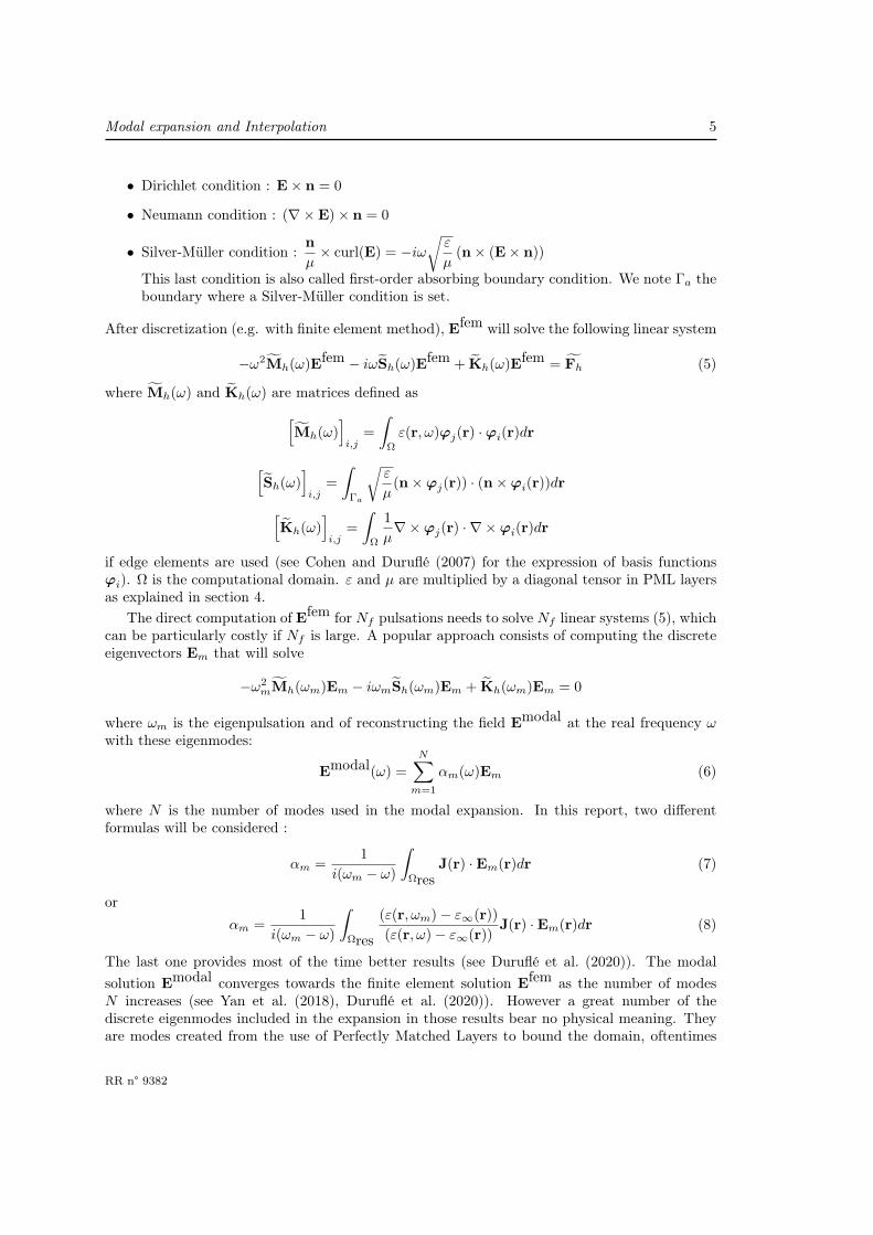
1 Introduction
Optical micro- and nanoresonators localize and enhance the electromagnetic energy at wavelengthand subwavelength scales and are a mainstay of many photonic devices. Their optical responseis characterized by resonant features resulting from the excitation of one or a few dominantmodes, intrinsic to the resonator. These modes of open, leaky resonator are oftentimes calledquasinormal modes (QNMs) to emphasize that their harmonic evolution is characterized by anexponential damping in time, due to the non-Hermitian nature of the corresponding scatteringoperatorLalanne et al. (2018).
In order to compute the electric field for a wide range of frequencies, an approach consistsof computing the modes characterizing the optical device, and expand the solution onto thesemodes :
E(r, ω) =∑m
αm(ω)Em(r, ω),
RR n° 9382

4 Duruflé & Gras & Lalanne
where Em is a mode, and αm(ω) the complex modal excitation coefficient. There exists differentformulas for the coefficients αm (see Lalanne et al. (2018) and Duruflé et al. (2020)). However, toreach a given accuracy, the number of modes used in the modal expansion can be very large (Yanet al. (2018), Duruflé et al. (2020)) whatever the used formula. We can cite the method developedin (Zimmerling et al., 2016) where the modes are computed simultaneously with the coefficientsαm such that only significant modes are kept in order to reduce this number of modes. Anotherapproach described in (Binkowski et al., 2019; Zschiedrich et al., 2018) relies on an integrationpath in the complex frequency plane which encloses the eigenmodes of interests. The scatteredfield at the real frequency can thus be expressed as a sum of two contributions : a resonantcontribution made up of contour integrals around the eigenfrequencies in the complex plane, anda non-resonant contribution, a setup that’s echoed in (Colom et al., 2018).
In this report, we will try to explain why the number of modes can be very large, this isthe object of the section 3. The limitations of the modal expansion (1) are sumarized in thesub-section 3.3. In order to overcome these limitations, we propose to interpolate the differencebetween the finite element solution and the modal solution. This difference is slowly varyingsuch that a polynomial interpolation converges fastly. This process is described in section 5 withnumerical results in 2-D and 3-D. In the section 4, we investigated different strategies to computeefficiently the eigenmodes Em (see Demésy et al. (2020) on the same topic). In the appendix A,the interpolation procedure is tested in the cases detailed in section 3. The appendix B dealswith the design of a permittivity function ε(ω) such that poles and roots are far from the realaxis.
2 General settingOur system is described by a permittivity distribution ε(r, ω). In this report, we consider a Padéapproximant of this permittivity that respects the causality principle as detailed in (Sehmi et al.,2017) :
ε(r, ω) =
ε∞ +
D∑d=1
iηkω + iγk
+
L∑k=1
(iσk
ω − Ωk+
iσkω + Ωk
), if r ∈ Ωres
εb otherwise
(1)
where σk and Ωk are complex coefficients and γk, ηk are real coefficients. Ωres is the domain ofthe resonator, εb is the background permittivity. In Duruflé et al. (2020), it is explained thatthe model (1) can be rewritten inside the resonator as
ε(r, ω) = ε∞ −L∑k=1
ck − iωσkω2 − ω2
0,k + iγkω, (2)
with real coefficients ck, σk, ω0,k, γk.The electric field Es solve the Maxwell’s equations
−ω2 ε(r, ω)Es +∇×∇×(µ−1Es
)= J(r, ω) (3)
where J is a source term and µ the magnetic permeability. When the scattered field is computed,we take
J(r, ω) = ω2 (ε(r, ω)− εb)Einc (4)
where εb is the background permittivity and Einc the incident field. We will consider threedifferent boundary conditions (n is the outgoing normale)
Inria
Modal expansion and Interpolation 5
• Dirichlet condition : E× n = 0
• Neumann condition : (∇×E)× n = 0
• Silver-Müller condition :nµ× curl(E) = −iω
√ε
µ(n× (E× n))
This last condition is also called first-order absorbing boundary condition. We note Γa theboundary where a Silver-Müller condition is set.
After discretization (e.g. with finite element method), Efem will solve the following linear system
−ω2Mh(ω)Efem − iωSh(ω)Efem + Kh(ω)Efem = Fh (5)
where Mh(ω) and Kh(ω) are matrices defined as[Mh(ω)
]i,j
=
∫Ω
ε(r, ω)ϕj(r) ·ϕi(r)dr
[Sh(ω)
]i,j
=
∫Γa
√ε
µ(n×ϕj(r)) · (n×ϕi(r))dr[
Kh(ω)]i,j
=
∫Ω
1
µ∇×ϕj(r) · ∇ ×ϕi(r)dr
if edge elements are used (see Cohen and Duruflé (2007) for the expression of basis functionsϕi). Ω is the computational domain. ε and µ are multiplied by a diagonal tensor in PML layersas explained in section 4.
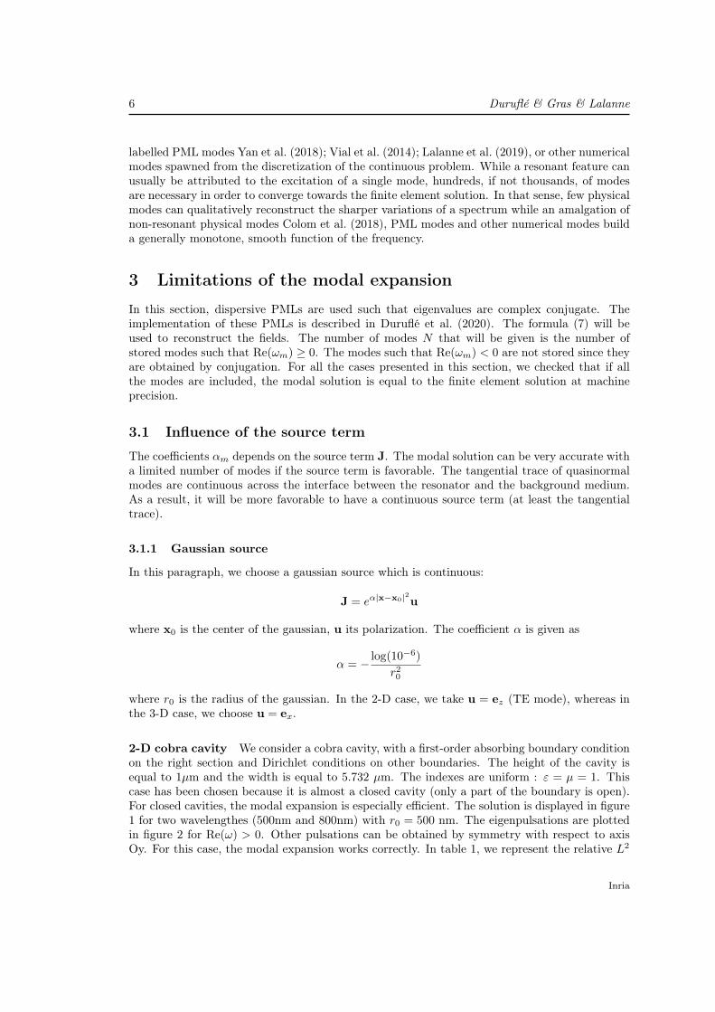
The direct computation of Efem for Nf pulsations needs to solve Nf linear systems (5), whichcan be particularly costly if Nf is large. A popular approach consists of computing the discreteeigenvectors Em that will solve
−ω2mMh(ωm)Em − iωmSh(ωm)Em + Kh(ωm)Em = 0
where ωm is the eigenpulsation and of reconstructing the field Emodal at the real frequency ωwith these eigenmodes:
Emodal(ω) =
N∑m=1
αm(ω)Em (6)
where N is the number of modes used in the modal expansion. In this report, two differentformulas will be considered :
αm =1
i(ωm − ω)
∫Ωres
J(r) ·Em(r)dr (7)
orαm =
1
i(ωm − ω)
∫Ωres
(ε(r, ωm)− ε∞(r))(ε(r, ω)− ε∞(r))
J(r) ·Em(r)dr (8)
The last one provides most of the time better results (see Duruflé et al. (2020)). The modalsolution Emodal converges towards the finite element solution Efem as the number of modesN increases (see Yan et al. (2018), Duruflé et al. (2020)). However a great number of thediscrete eigenmodes included in the expansion in those results bear no physical meaning. Theyare modes created from the use of Perfectly Matched Layers to bound the domain, oftentimes
RR n° 9382
6 Duruflé & Gras & Lalanne
labelled PML modes Yan et al. (2018); Vial et al. (2014); Lalanne et al. (2019), or other numericalmodes spawned from the discretization of the continuous problem. While a resonant feature canusually be attributed to the excitation of a single mode, hundreds, if not thousands, of modesare necessary in order to converge towards the finite element solution. In that sense, few physicalmodes can qualitatively reconstruct the sharper variations of a spectrum while an amalgation ofnon-resonant physical modes Colom et al. (2018), PML modes and other numerical modes builda generally monotone, smooth function of the frequency.
3 Limitations of the modal expansion
In this section, dispersive PMLs are used such that eigenvalues are complex conjugate. Theimplementation of these PMLs is described in Duruflé et al. (2020). The formula (7) will beused to reconstruct the fields. The number of modes N that will be given is the number ofstored modes such that Re(ωm) ≥ 0. The modes such that Re(ωm) < 0 are not stored since theyare obtained by conjugation. For all the cases presented in this section, we checked that if allthe modes are included, the modal solution is equal to the finite element solution at machineprecision.
3.1 Influence of the source term
The coefficients αm depends on the source term J. The modal solution can be very accurate witha limited number of modes if the source term is favorable. The tangential trace of quasinormalmodes are continuous across the interface between the resonator and the background medium.As a result, it will be more favorable to have a continuous source term (at least the tangentialtrace).
3.1.1 Gaussian source
In this paragraph, we choose a gaussian source which is continuous:
J = eα|x−x0|2u
where x0 is the center of the gaussian, u its polarization. The coefficient α is given as
α = − log(10−6)
r20
where r0 is the radius of the gaussian. In the 2-D case, we take u = ez (TE mode), whereas inthe 3-D case, we choose u = ex.
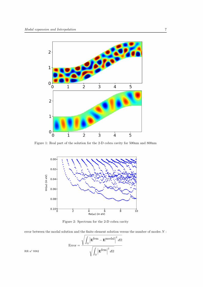
2-D cobra cavity We consider a cobra cavity, with a first-order absorbing boundary conditionon the right section and Dirichlet conditions on other boundaries. The height of the cavity isequal to 1µm and the width is equal to 5.732 µm. The indexes are uniform : ε = µ = 1. Thiscase has been chosen because it is almost a closed cavity (only a part of the boundary is open).For closed cavities, the modal expansion is especially efficient. The solution is displayed in figure1 for two wavelengthes (500nm and 800nm) with r0 = 500 nm. The eigenpulsations are plottedin figure 2 for Re(ω) > 0. Other pulsations can be obtained by symmetry with respect to axisOy. For this case, the modal expansion works correctly. In table 1, we represent the relative L2
Inria
Modal expansion and Interpolation 7
Figure 1: Real part of the solution for the 2-D cobra cavity for 500nm and 800nm
0 2 4 6 8 10Re(ω) (in eV)
−0.10
−0.08
−0.06
−0.04
−0.02
0.00
Im(ω
) (in eV)
Figure 2: Spectrum for the 2-D cobra cavity
error between the modal solution and the finite element solution versus the number of modes N :
Error =
√∫Ω
∣∣∣Efem −Emodal∣∣∣2 dΩ√∫
Ω
∣∣∣Efem∣∣∣2 dΩRR n° 9382
8 Duruflé & Gras & Lalanne
This error is computed for 201 angular frequencies (between 1.24eV and 2.48eV which correspondsto wavelengthes between 500nm and 800nm) and we select the maximal error. We select modes
L (in eV) 1.97 2.96 3.95 4.93 5.92 6.91 7.89N 39 91 174 272 406 558 732
Error (r0=500nm) 1.0089 0.0671 0.01044 2.572 · 10−3 4.796 · 10−4 9.934 · 10−5 1.4436 · 10−5
Error (r0=250nm) 1.0106 0.1027 0.03655 0.019143 0.009563 0.005576 0.00296
Table 1: Relative L2 error for the 2-D cobra cavity.
such that |Re(ωm)| < L, the values of L are also given in this table. We observe that bydecreasing the radius r0, the error will increase. The reason is that a narrower gaussian willexcite more high-frequency modes. The numerical error obtained for the used mesh is below10−5. We observe that the modal expansion needs to compute the eigenpulsations until 7.89 eVto reach this error. This value is much larger than 2.48eV (the maximal frequency considered)and induces to compute a large number of modes to obtain a solution as accurate as the finiteelement solution.
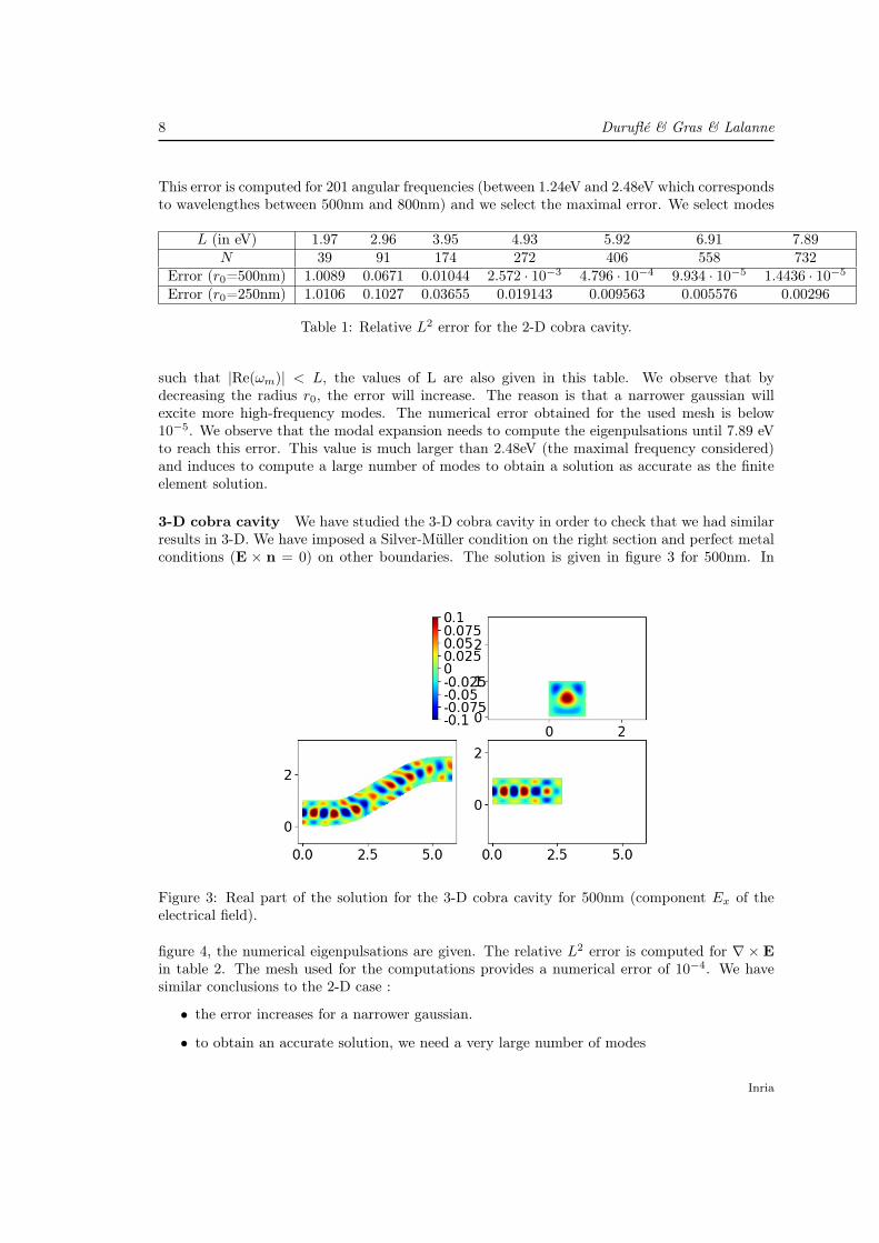
3-D cobra cavity We have studied the 3-D cobra cavity in order to check that we had similarresults in 3-D. We have imposed a Silver-Müller condition on the right section and perfect metalconditions (E × n = 0) on other boundaries. The solution is given in figure 3 for 500nm. In
Figure 3: Real part of the solution for the 3-D cobra cavity for 500nm (component Ex of theelectrical field).
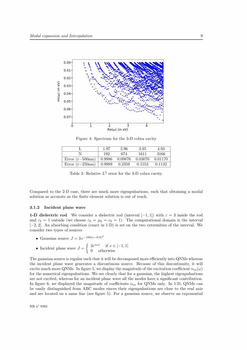
figure 4, the numerical eigenpulsations are given. The relative L2 error is computed for ∇ × Ein table 2. The mesh used for the computations provides a numerical error of 10−4. We havesimilar conclusions to the 2-D case :
• the error increases for a narrower gaussian.
• to obtain an accurate solution, we need a very large number of modes
Inria
Modal expansion and Interpolation 9
0 1 2 3 4Re(ω) (in eV)
−0.07
−0.06
−0.05
−0.04
−0.03
−0.02
−0.01
0.00Im
(ω) (in eV)
Figure 4: Spectrum for the 3-D cobra cavity
L 1.97 2.96 3.95 4.93N 192 674 1611 3166
Error (r=500nm) 0.9986 0.09876 0.03070 0.01170Error (r=250nm) 0.9989 0.2359 0.1553 0.1132
Table 2: Relative L2 error for the 3-D cobra cavity.
Compared to the 2-D case, there are much more eigenpulsations, such that obtaining a modalsolution as accurate as the finite element solution is out of reach.
3.1.2 Incident plane wave
1-D dielectric rod We consider a dielectric rod (interval [−1, 1]) with ε = 3 inside the rodand εb = 1 outside (we choose ε0 = µ0 = c0 = 1). The computational domain is the interval[−2, 2]. An absorbing condition (exact in 1-D) is set on the two extremities of the interval. Weconsider two types of sources
• Gaussian source J = 3 e−100(x−0.6)2
• Incident plane wave J =
2eiωx if x ∈ [−1, 1]0 otherwise
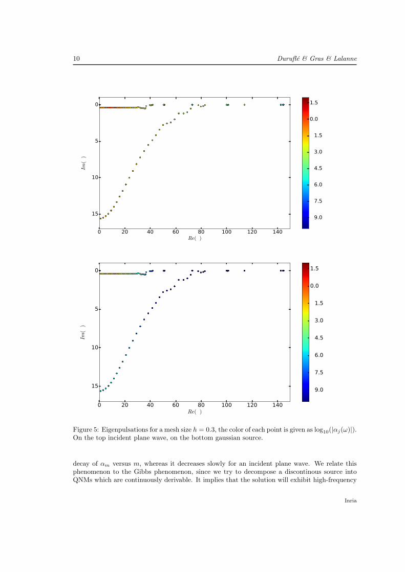
The gaussian source is regular such that it will be decomposed more efficiently into QNMs whereasthe incident plane wave generates a discontinous source. Because of this discontinuity, it willexcite much more QNMs. In figure 5, we display the magnitude of the excitation coefficient αm(ω)for the numerical eigenpulsations. We see clearly that for a gaussian, the highest eigenpulsationsare not excited, whereas for an incident plane wave all the modes have a significant contribution.In figure 6, we displayed the magnitude of coefficients αm for QNMs only. In 1-D, QNMs canbe easily distinguished from ABC modes sinces their eigenpulsations are close to the real axisand are located on a same line (see figure 5). For a gaussian source, we observe an exponential
RR n° 9382
10 Duruflé & Gras & Lalanne
0 20 40 60 80 100 120 140Re(ω)
−15
−10
−5
0
Im(ω
)
−9.0
−7.5
−6.0
−4.5
−3.0
−1.5
0.0
1.5
0 20 40 60 80 100 120 140Re(ω)
−15
−10
−5
0
Im(ω
)
−9.0
−7.5
−6.0
−4.5
−3.0
−1.5
0.0
1.5
Figure 5: Eigenpulsations for a mesh size h = 0.3, the color of each point is given as log10(|αj(ω)|).On the top incident plane wave, on the bottom gaussian source.
decay of αm versus m, whereas it decreases slowly for an incident plane wave. We relate thisphenomenon to the Gibbs phenomenon, since we try to decompose a discontinous source intoQNMs which are continuously derivable. It implies that the solution will exhibit high-frequency
Inria
Modal expansion and Interpolation 11
0 5 10 15 20 25 30 35 40 45N
10-8
10-7
10-6
10-5
10-4
10-3
10-2
10-1
100|α
j(ω
)|
Incident plane wave
Gaussian
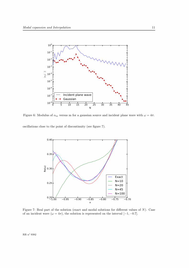
Figure 6: Modulus of αm versus m for a gaussian source and incident plane wave with ω = 4π.
oscillations close to the point of discontinuity (see figure 7).
−1.00 −0.95 −0.90 −0.85 −0.80 −0.75 −0.70x
0.20
0.25
0.30
0.35
0.40
Re(u)
Exact
N=10
N=20
N=45
N=100
Figure 7: Real part of the solution (exact and modal solutions for different values of N). Caseof an incident wave (ω = 4π), the solution is represented on the interval [−1,−0.7].
RR n° 9382
12 Duruflé & Gras & Lalanne
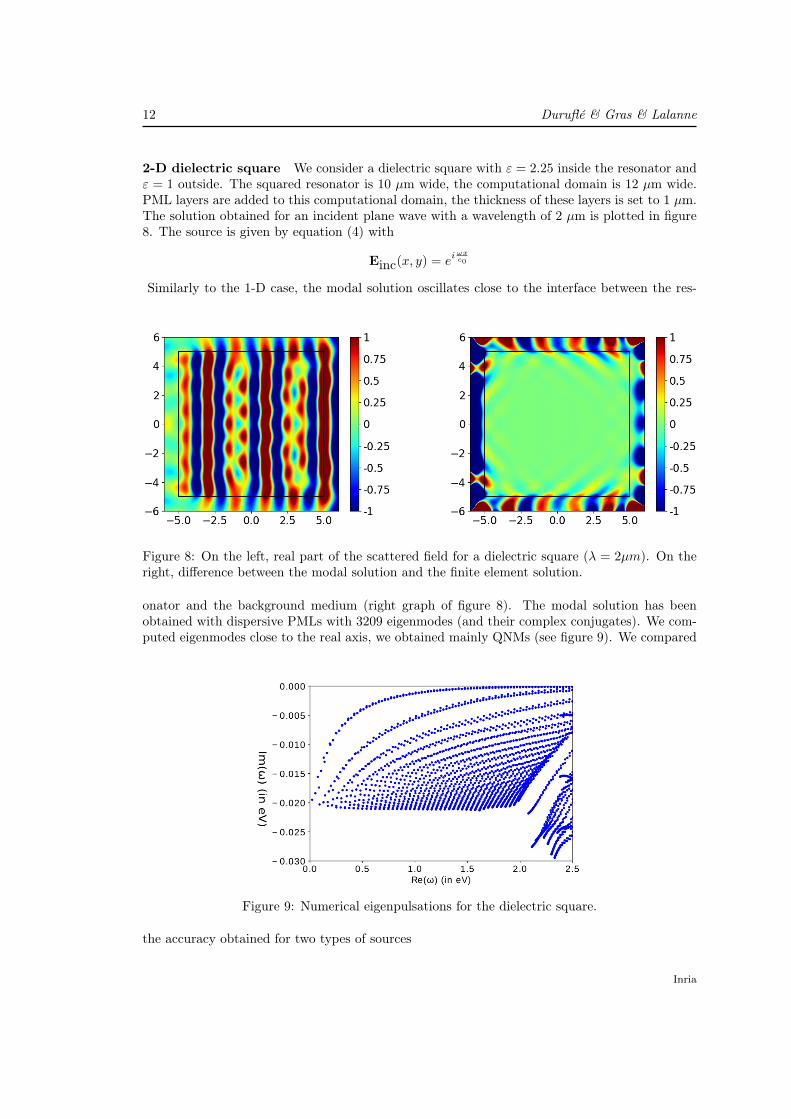
2-D dielectric square We consider a dielectric square with ε = 2.25 inside the resonator andε = 1 outside. The squared resonator is 10 µm wide, the computational domain is 12 µm wide.PML layers are added to this computational domain, the thickness of these layers is set to 1 µm.The solution obtained for an incident plane wave with a wavelength of 2 µm is plotted in figure8. The source is given by equation (4) with
Einc(x, y) = eiωxc0
Similarly to the 1-D case, the modal solution oscillates close to the interface between the res-
Figure 8: On the left, real part of the scattered field for a dielectric square (λ = 2µm). On theright, difference between the modal solution and the finite element solution.
onator and the background medium (right graph of figure 8). The modal solution has beenobtained with dispersive PMLs with 3209 eigenmodes (and their complex conjugates). We com-puted eigenmodes close to the real axis, we obtained mainly QNMs (see figure 9). We compared
Figure 9: Numerical eigenpulsations for the dielectric square.
the accuracy obtained for two types of sources
Inria
Modal expansion and Interpolation 13
• Gaussian source (r0 = 1.25µm)
• Incident plane wave
N 784 1027 1969 3209Plane wave 0.238644 0.137773 0.0859191 0.085545Gaussian 0.155995 0.049234 0.020971 0.020966
Table 3: Relative L2 error inside the resonator between the modal solution and the finite elementsolution versus the number od modes N . Case of the dielectric square.
We have computed the L2 error inside the resonator for these two types of source (see table 3).We see that we obtain a better accuracy for the gaussian source as expected. For this case, wesee also that increasing the number of modes does not necessarily improve the solution. For thiscase, with 1969 or 3209 modes, the accuracy is similar.
3.2 Dispersive materials3.2.1 Germanium disk
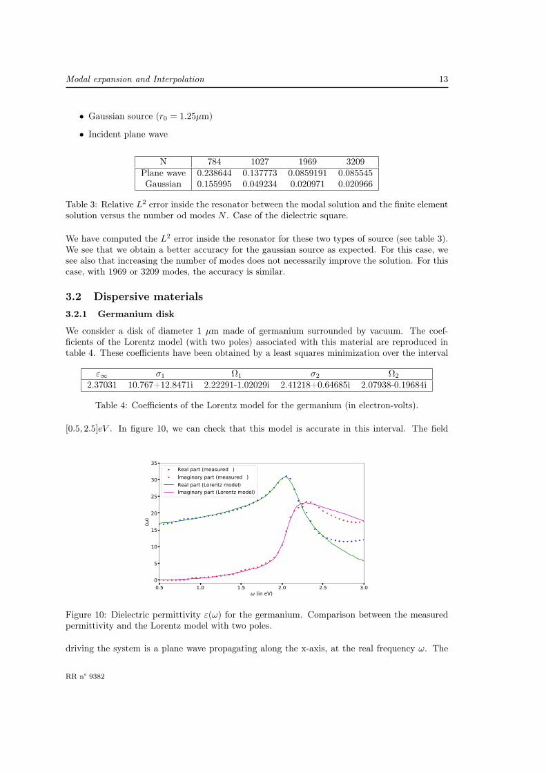
We consider a disk of diameter 1 µm made of germanium surrounded by vacuum. The coef-ficients of the Lorentz model (with two poles) associated with this material are reproduced intable 4. These coefficients have been obtained by a least squares minimization over the interval
ε∞ σ1 Ω1 σ2 Ω2
2.37031 10.767+12.8471i 2.22291-1.02029i 2.41218+0.64685i 2.07938-0.19684i
Table 4: Coefficients of the Lorentz model for the germanium (in electron-volts).
[0.5, 2.5]eV . In figure 10, we can check that this model is accurate in this interval. The field
0.5 1.0 1.5 2.0 2.5 3.0ω (in eV)
0
5
10
15
20
25
30
35
ε(ω)
Real part (measured ε)Imaginary part (measured ε)Real part (Lorentz model)Imaginary part (Lorentz model)
Figure 10: Dielectric permittivity ε(ω) for the germanium. Comparison between the measuredpermittivity and the Lorentz model with two poles.
driving the system is a plane wave propagating along the x-axis, at the real frequency ω. The
RR n° 9382
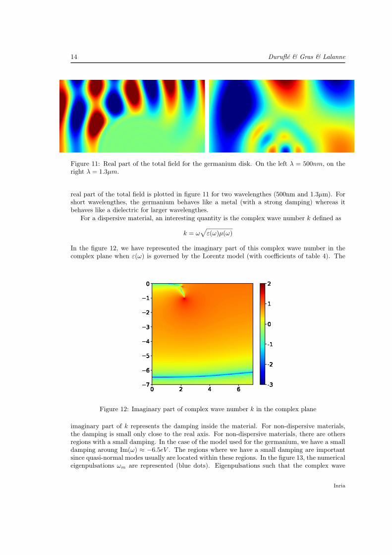
14 Duruflé & Gras & Lalanne
Figure 11: Real part of the total field for the germanium disk. On the left λ = 500nm, on theright λ = 1.3µm.
real part of the total field is plotted in figure 11 for two wavelengthes (500nm and 1.3µm). Forshort wavelengthes, the germanium behaves like a metal (with a strong damping) whereas itbehaves like a dielectric for larger wavelengthes.
For a dispersive material, an interesting quantity is the complex wave number k defined as
k = ω√ε(ω)µ(ω)
In the figure 12, we have represented the imaginary part of this complex wave number in thecomplex plane when ε(ω) is governed by the Lorentz model (with coefficients of table 4). The
Figure 12: Imaginary part of complex wave number k in the complex plane
imaginary part of k represents the damping inside the material. For non-dispersive materials,the damping is small only close to the real axis. For non-dispersive materials, there are othersregions with a small damping. In the case of the model used for the germanium, we have a smalldamping aroung Im(ω) ≈ −6.5eV . The regions where we have a small damping are importantsince quasi-normal modes usually are located within these regions. In the figure 13, the numericaleigenpulsations ωm are represented (blue dots). Eigenpulsations such that the complex wave
Inria
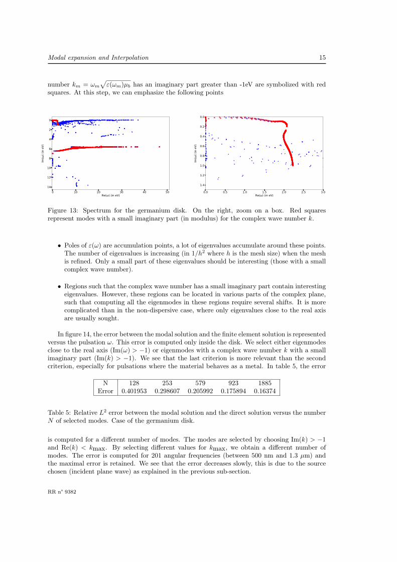
Modal expansion and Interpolation 15
number km = ωm√ε(ωm)µb has an imaginary part greater than -1eV are symbolized with red
squares. At this step, we can emphasize the following points
0 10 20 30 40 50Re(ω) (in eV)
−14
−12
−10
−8
−6
−4
−2
0
Im(ω
) (in eV)
0.0 0.5 1.0 1.5 2.0 2.5 3.0Re(ω) (in eV)
−1.4
−1.2
−1.0
−0.8
−0.6
−0.4
−0.2
0.0
Im(ω
) (in eV)
Figure 13: Spectrum for the germanium disk. On the right, zoom on a box. Red squaresrepresent modes with a small imaginary part (in modulus) for the complex wave number k.
• Poles of ε(ω) are accumulation points, a lot of eigenvalues accumulate around these points.The number of eigenvalues is increasing (in 1/h2 where h is the mesh size) when the meshis refined. Only a small part of these eigenvalues should be interesting (those with a smallcomplex wave number).
• Regions such that the complex wave number has a small imaginary part contain interestingeigenvalues. However, these regions can be located in various parts of the complex plane,such that computing all the eigenmodes in these regions require several shifts. It is morecomplicated than in the non-dispersive case, where only eigenvalues close to the real axisare usually sought.
In figure 14, the error between the modal solution and the finite element solution is representedversus the pulsation ω. This error is computed only inside the disk. We select either eigenmodesclose to the real axis (Im(ω) > −1) or eigenmodes with a complex wave number k with a smallimaginary part (Im(k) > −1). We see that the last criterion is more relevant than the secondcriterion, especially for pulsations where the material behaves as a metal. In table 5, the error
N 128 253 579 923 1885Error 0.401953 0.298607 0.205992 0.175894 0.16374
Table 5: Relative L2 error between the modal solution and the direct solution versus the numberN of selected modes. Case of the germanium disk.
is computed for a different number of modes. The modes are selected by choosing Im(k) > −1and Re(k) < kmax. By selecting different values for kmax, we obtain a different number ofmodes. The error is computed for 201 angular frequencies (between 500 nm and 1.3 µm) andthe maximal error is retained. We see that the error decreases slowly, this is due to the sourcechosen (incident plane wave) as explained in the previous sub-section.
RR n° 9382
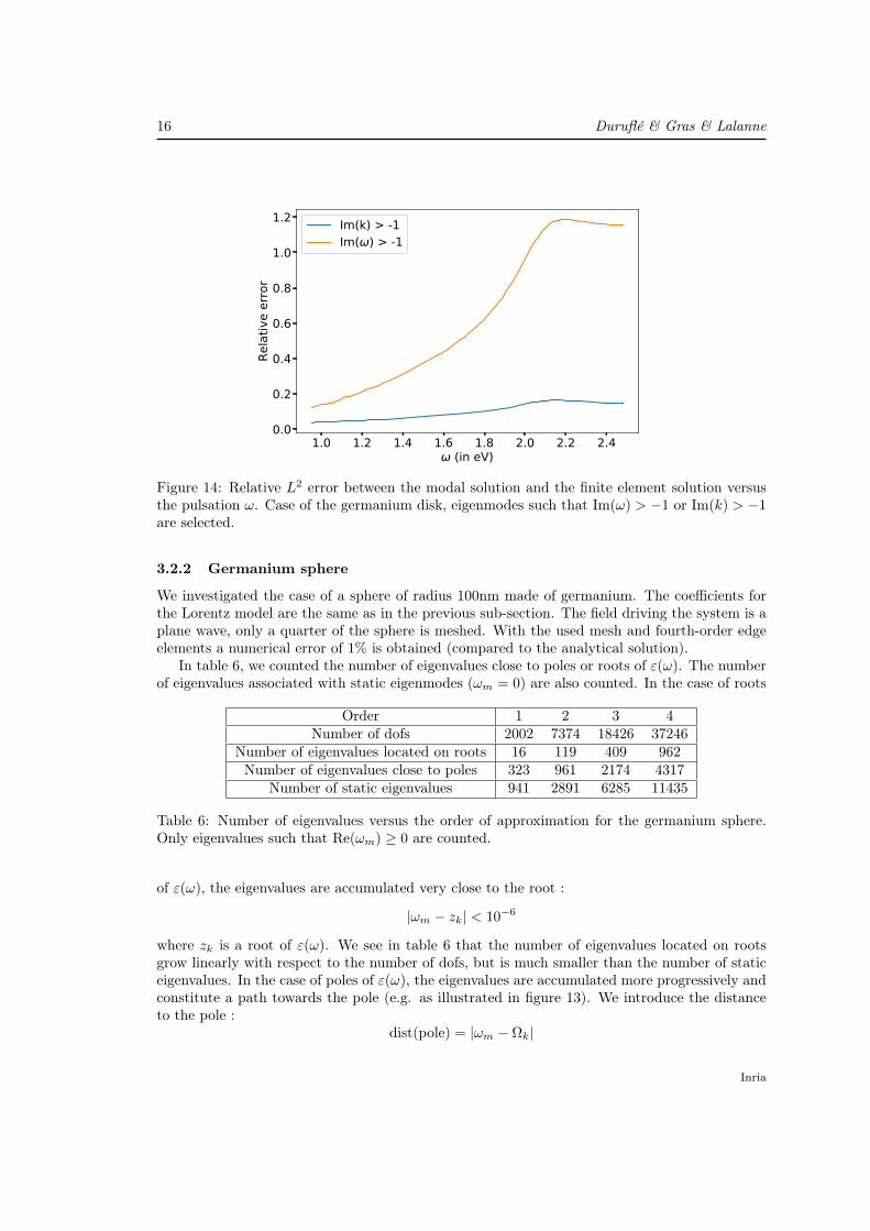
16 Duruflé & Gras & Lalanne
1.0 1.2 1.4 1.6 1.8 2.0 2.2 2.4ω (in eV)
0.0
0.2
0.4
0.6
0.8
1.0
1.2
Relativ
e error
Im(k) > -1Im(ω) > -1
Figure 14: Relative L2 error between the modal solution and the finite element solution versusthe pulsation ω. Case of the germanium disk, eigenmodes such that Im(ω) > −1 or Im(k) > −1are selected.
3.2.2 Germanium sphere
We investigated the case of a sphere of radius 100nm made of germanium. The coefficients forthe Lorentz model are the same as in the previous sub-section. The field driving the system is aplane wave, only a quarter of the sphere is meshed. With the used mesh and fourth-order edgeelements a numerical error of 1% is obtained (compared to the analytical solution).
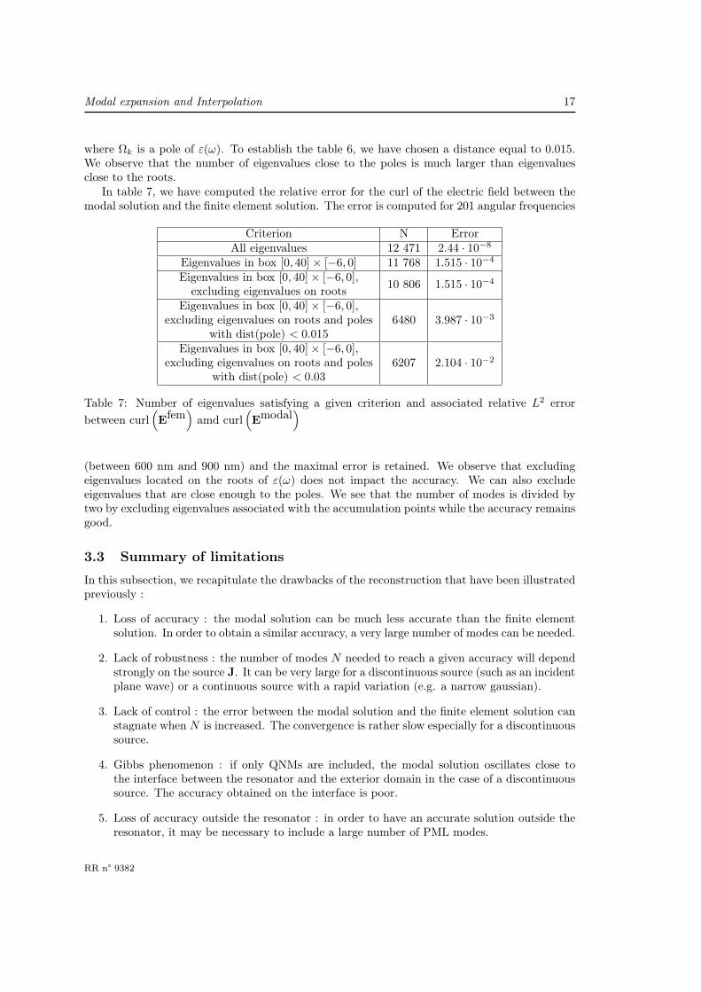
In table 6, we counted the number of eigenvalues close to poles or roots of ε(ω). The numberof eigenvalues associated with static eigenmodes (ωm = 0) are also counted. In the case of roots
Order 1 2 3 4Number of dofs 2002 7374 18426 37246
Number of eigenvalues located on roots 16 119 409 962Number of eigenvalues close to poles 323 961 2174 4317
Number of static eigenvalues 941 2891 6285 11435
Table 6: Number of eigenvalues versus the order of approximation for the germanium sphere.Only eigenvalues such that Re(ωm) ≥ 0 are counted.
of ε(ω), the eigenvalues are accumulated very close to the root :
|ωm − zk| < 10−6
where zk is a root of ε(ω). We see in table 6 that the number of eigenvalues located on rootsgrow linearly with respect to the number of dofs, but is much smaller than the number of staticeigenvalues. In the case of poles of ε(ω), the eigenvalues are accumulated more progressively andconstitute a path towards the pole (e.g. as illustrated in figure 13). We introduce the distanceto the pole :
dist(pole) = |ωm − Ωk|
Inria
Modal expansion and Interpolation 17
where Ωk is a pole of ε(ω). To establish the table 6, we have chosen a distance equal to 0.015.We observe that the number of eigenvalues close to the poles is much larger than eigenvaluesclose to the roots.
In table 7, we have computed the relative error for the curl of the electric field between themodal solution and the finite element solution. The error is computed for 201 angular frequencies
Criterion N ErrorAll eigenvalues 12 471 2.44 · 10−8
Eigenvalues in box [0, 40]× [−6, 0] 11 768 1.515 · 10−4
Eigenvalues in box [0, 40]× [−6, 0],excluding eigenvalues on roots 10 806 1.515 · 10−4
Eigenvalues in box [0, 40]× [−6, 0],excluding eigenvalues on roots and poles
with dist(pole) < 0.0156480 3.987 · 10−3
Eigenvalues in box [0, 40]× [−6, 0],excluding eigenvalues on roots and poles
with dist(pole) < 0.036207 2.104 · 10−2
Table 7: Number of eigenvalues satisfying a given criterion and associated relative L2 errorbetween curl
(Efem
)amd curl
(Emodal
)
(between 600 nm and 900 nm) and the maximal error is retained. We observe that excludingeigenvalues located on the roots of ε(ω) does not impact the accuracy. We can also excludeeigenvalues that are close enough to the poles. We see that the number of modes is divided bytwo by excluding eigenvalues associated with the accumulation points while the accuracy remainsgood.
3.3 Summary of limitations
In this subsection, we recapitulate the drawbacks of the reconstruction that have been illustratedpreviously :
1. Loss of accuracy : the modal solution can be much less accurate than the finite elementsolution. In order to obtain a similar accuracy, a very large number of modes can be needed.
2. Lack of robustness : the number of modes N needed to reach a given accuracy will dependstrongly on the source J. It can be very large for a discontinuous source (such as an incidentplane wave) or a continuous source with a rapid variation (e.g. a narrow gaussian).
3. Lack of control : the error between the modal solution and the finite element solution canstagnate when N is increased. The convergence is rather slow especially for a discontinuoussource.
4. Gibbs phenomenon : if only QNMs are included, the modal solution oscillates close tothe interface between the resonator and the exterior domain in the case of a discontinuoussource. The accuracy obtained on the interface is poor.
5. Loss of accuracy outside the resonator : in order to have an accurate solution outside theresonator, it may be necessary to include a large number of PML modes.
RR n° 9382
18 Duruflé & Gras & Lalanne
6. Need to compute eigenvalues in different parts of the complex plane :
(a) In the non-dispersive case, we would like to compute only eigenvalues close to theinterval [ω1, ω2] on the real axis, since the solution will be reconstructed on this in-terval. However, it is actually necessary to compute modes on a larger zone withRe(ω) >> ω2 due to Gibbs phenomenon.
(b) In the case of dispersive materials, the complex wave number ω√ε(ω)µ can have
a small imaginary part in different regions of the complex plane (depending on thelocations of roots of ε(ω)). To obtain an accurate modal solution, it is not sufficientto consider only eigenvalues close to the interval [ω1, ω2] of the real axis.
7. Presence of accumulation points : for a dispersive material, poles and zeros of ε(ω) areaccumulation points for the eigenvalues. In the case of a geometry with corners the solutionsof ε(ω) = −1 are also accumulation points. The number of eigenvalues near these pointsincreases linearly with respect to the number of degrees of freedom. Most of the eigenmodes(especially when the eigenvalues are very close to the accumulation point) do not contributesignificantly to the modal solution. However, the eigensolver can fail if the number of theseeigenvalues is larger than the number of requested eigenvalues. These eigenvalues can also"hide" significant eigenvalues if the shift used to compute eigenvalues is not well located.
4 Efficient Computation of eigenmodesIn this section, we investigate different methods to compute efficiently eigenmodes. The aim isto select the best method in order to have an efficient reconstruction.
4.1 Dispersive PMLsDispersive PMLs consist of multiplying ε and µ by the following diagonal tensor
C(ω) =(−iω + T2,3,1) (−iω + T3,1,2)
−iω (−iω + T1,2,3)
where
Ti,j,k =
σi 0 00 σj 00 0 σk
The damping coefficients σx, σy and σz inside a PML where x > x0, y > y0 or z > z0 areparabolic:
σ1 = σx =3 log(1000)
2a3(x− x0)2vmax σ
σ2 = σy =3 log(1000)
2a3(y − y0)2vmax σ
σ3 = σz =3 log(1000)
2a3(z − z0)2vmax σ.
The coefficient σ serves to adjust the reflection coefficient of the PML. vmax is the speed of thewave inside the PML and a is the thickness of PML layer. To implement, these PMLs, auxiliaryfields are added such that the eigenvalue problem is linear :
Find ωm ∈ C and U 6= 0 such that
−iωmMhU + KhU = 0(9)
Inria
Modal expansion and Interpolation 19
where the matrices Mh and Kh are real and do not depend on the eigenvalue value λm = iωm.This process is detailed in (Duruflé et al., 2020). To solve the linear eigenvalue problem (9),we can use either Slepc or Arpack. For Arpack, we use the routine dneupd (for real matrices)with a complex shift. For Slepc, we use the solver EPS with complex numbers. A spectraltransformation is used such that largest eigenvalues of (Kh − σMh)
−1 Mh are sought to obtainthe eigenvalues closest to the shift σ. In order to factorize the matrix Kh − σMh, the directsolver MUMPs is used (Amestoy et al. (2001)). A static condensation procedure (see chapter 3of N’diaye (2017)) is performed in order to factorize a reduced linear system (auxiliary unknownsand internal degrees of freedom are removed). When Arpack is used, 2N eigenvalues are askedsince the routine dneupd will compute complex conjugate eigenvalues. As a result N eigenvaluesare obtained close to the shift σ and N eigenvalues are obtained close to σ. When Slepc is used,N eigenvalues are asked since it will compute N eigenvalues close to the complex shift σ (withoutcomputing the eigenvalues close to σ).
4.2 Non-dispersive PMLsIn the case of non-dispersive PMLs, ε and µ are multiplied by C(ω0) where ω0 is a given fre-quency usually chosen in the interval [ω1, ω2] where the solution will be reconstructed. Maxwell’sequations are written in the form
−ω2C(ω0) (ε∞E +∑kPk)− curl
(1
µbC(ω0)curlE
)= 0
−ω2Pk − iωγkPk + ω20,kPk = ck − iωσkE
After discretization, we obtain a quadratic eigenvalue problemFind ωm ∈ C and U 6= 0 such that
−ω2mMhU− iωmShU + KhU = 0
(10)
where Mh,Sh and Kh are complex matrices. To solve this polynomial eigenvalue problem,we use PEP solver proposed in Slepc. As described in Campos and Roman (2016), a spectraltransformation is used such that largest eigenvalues θ of the quadratic eigenvalue problem
θ2(Kh − σSh − σ2Mh
)x− θ (Sh + 2σMh)x−Mhx = 0
are sought, and eigenvalues λm = iωm closest to the shift σ are obtained as
λm = σ +1
θ
The matrix(Kh − σSh − σ2Mh
)is factorized with Mumps. A static condensation procedure
is also used in order to factorize a reduced linear system. For both cases (dispersive or non-dispersive PMLs), this linear system has the same size.
4.3 Comparison of solversWe compare the following solvers
• Dispersive PMLs + Arpack
• Dispersive PMLs + Slepc
RR n° 9382
20 Duruflé & Gras & Lalanne
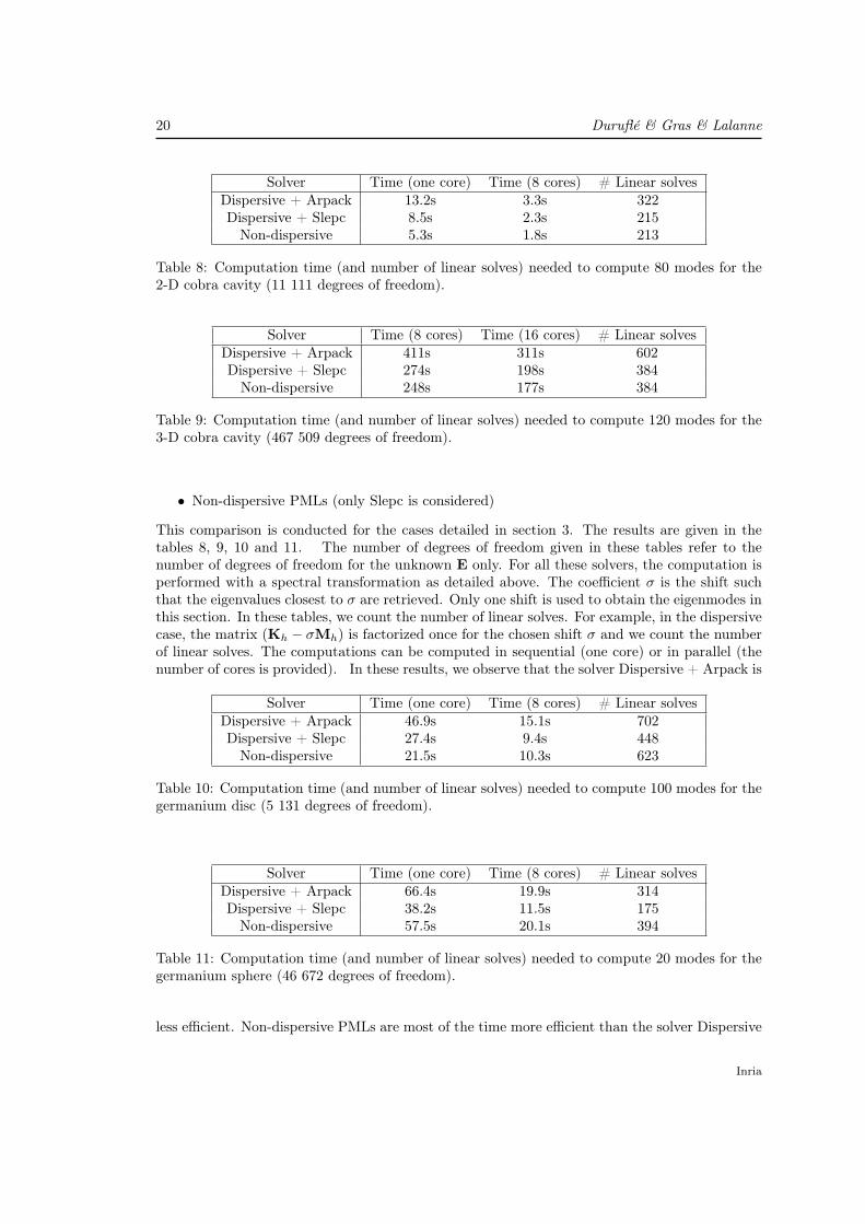
Solver Time (one core) Time (8 cores) # Linear solvesDispersive + Arpack 13.2s 3.3s 322Dispersive + Slepc 8.5s 2.3s 215Non-dispersive 5.3s 1.8s 213
Table 8: Computation time (and number of linear solves) needed to compute 80 modes for the2-D cobra cavity (11 111 degrees of freedom).
Solver Time (8 cores) Time (16 cores) # Linear solvesDispersive + Arpack 411s 311s 602Dispersive + Slepc 274s 198s 384Non-dispersive 248s 177s 384
Table 9: Computation time (and number of linear solves) needed to compute 120 modes for the3-D cobra cavity (467 509 degrees of freedom).
• Non-dispersive PMLs (only Slepc is considered)
This comparison is conducted for the cases detailed in section 3. The results are given in thetables 8, 9, 10 and 11. The number of degrees of freedom given in these tables refer to thenumber of degrees of freedom for the unknown E only. For all these solvers, the computation isperformed with a spectral transformation as detailed above. The coefficient σ is the shift suchthat the eigenvalues closest to σ are retrieved. Only one shift is used to obtain the eigenmodes inthis section. In these tables, we count the number of linear solves. For example, in the dispersivecase, the matrix (Kh − σMh) is factorized once for the chosen shift σ and we count the numberof linear solves. The computations can be computed in sequential (one core) or in parallel (thenumber of cores is provided). In these results, we observe that the solver Dispersive + Arpack is
Solver Time (one core) Time (8 cores) # Linear solvesDispersive + Arpack 46.9s 15.1s 702Dispersive + Slepc 27.4s 9.4s 448Non-dispersive 21.5s 10.3s 623
Table 10: Computation time (and number of linear solves) needed to compute 100 modes for thegermanium disc (5 131 degrees of freedom).
Solver Time (one core) Time (8 cores) # Linear solvesDispersive + Arpack 66.4s 19.9s 314Dispersive + Slepc 38.2s 11.5s 175Non-dispersive 57.5s 20.1s 394
Table 11: Computation time (and number of linear solves) needed to compute 20 modes for thegermanium sphere (46 672 degrees of freedom).
less efficient. Non-dispersive PMLs are most of the time more efficient than the solver Dispersive
Inria
Modal expansion and Interpolation 21
+ Slepc. But it may occur (cf. table 11) that the solver Dispersive + Slepc requires much lessiterations inducing a smaller computation time.
5 Interpolation procedure to reconstruct the fieldIn this section, we propose an interpolation strategy in order to overcome the encountered lim-itations in section 3. We denote u(r, ω) the difference between the finite element solution andthe modal expansion:
u(r, ω) = Efem(r, ω)−Emodal(r, ω) = Efem(r, ω)−N∑m=1
αm(ω)Em(r). (11)
We consider real frequencies ω within the range [ω1, ω2]. If we include N eigenmodes such thatall the resonances within the spectra are accounted for, then the difference u(r, ω) is a slowlyvarying function within [ω1, ω2]. It can thus be conveniently approximated by a polynomial inω.
We choose Ni interpolation points scattered within [ω1, ω2]:
ωk = ω1 + xk(ω2 − ω1), (12)
where xk are points over the interval [0, 1]. Many set of interpolation points can be used for anefficient interpolation, we have investigated three families of points:
• Chebyshev points: xk = 12 + 1
2 cos
(2k − 1
2Niπ
), k = 1..Ni
• Clenshaw-Curtis points: xk = 12 + 1
2 cos
(k − 1
Ni − 1π
), k = 1..Ni
• Leja points defined recursively as (see P. Jantsch (2016)):
xk = argmaxx∈[0,1]
k−1∏i=1
|x− xi|, k > 1
with x1 = 12 .
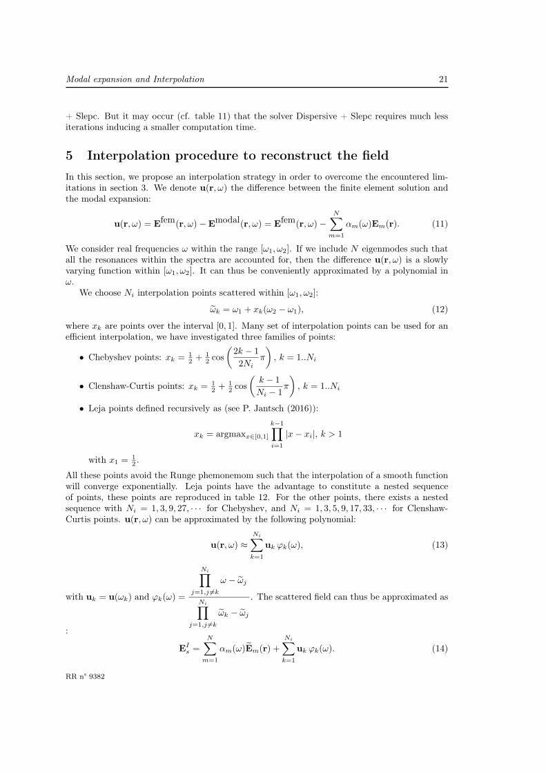
All these points avoid the Runge phemonemom such that the interpolation of a smooth functionwill converge exponentially. Leja points have the advantage to constitute a nested sequenceof points, these points are reproduced in table 12. For the other points, there exists a nestedsequence with Ni = 1, 3, 9, 27, · · · for Chebyshev, and Ni = 1, 3, 5, 9, 17, 33, · · · for Clenshaw-Curtis points. u(r, ω) can be approximated by the following polynomial:
u(r, ω) ≈Ni∑k=1
uk ϕk(ω), (13)
with uk = u(ωk) and ϕk(ω) =
Ni∏j=1,j 6=k
ω − ωj
Ni∏j=1,j 6=k
ωk − ωj
. The scattered field can thus be approximated as
:
EIs =
N∑m=1
αm(ω)Em(r) +
Ni∑k=1
uk ϕk(ω). (14)
RR n° 9382
22 Duruflé & Gras & Lalanne
x1 x2 x3 x4 x5 x6 x7 x8
0.5 0 1 0.2113248 0.8293532 0.0803729 0.9350035 0.6528066
x9 x10 x11 x12 x13 x14
0.3391461 0.0285104 0.9763366 0.7397061 0.1436806 0.4220203
x15 x16 x17 x18 x19 x20 x21
0.8874361 0.0102611 0.5805826 0.9916631 0.26931469 0.0540535 0.7859485
Table 12: Leja points xi (until i = 21). Only seven first digits are reproduced.
We can observe that any formula for αm (e.g. given by the equation (7) or (8)) can be writtenas
αm(ω) =1
i(ωm − ω)
∫Ω
J(ωm) ·Emdx+ β0 + β1(ω − ωm) + β2(ω − ωm)2 + · · ·
In this expression, the first term is a singular part (equal to the residue of αm(ω) divided byωm − ω) whereas other terms constitute a regular part. The different formulas for αm have thesame singular part but the regular part (coefficients βi) will differ. As a result, we numericallyobserve that the convergence of EIs towards the finite element solution Efem almost does notdepend on the chosen formula for αm. In this section, we will use the formula (8), but the resultsare very similar with other formulas.
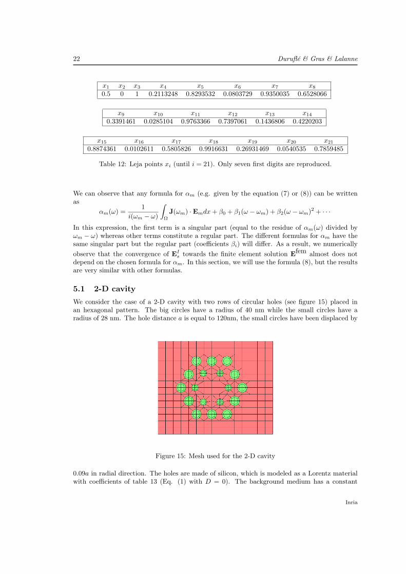
5.1 2-D cavityWe consider the case of a 2-D cavity with two rows of circular holes (see figure 15) placed inan hexagonal pattern. The big circles have a radius of 40 nm while the small circles have aradius of 28 nm. The hole distance a is equal to 120nm, the small circles have been displaced by
Figure 15: Mesh used for the 2-D cavity
0.09a in radial direction. The holes are made of silicon, which is modeled as a Lorentz materialwith coefficients of table 13 (Eq. (1) with D = 0). The background medium has a constant
Inria
Modal expansion and Interpolation 23
permittivity εb = 4. The field driving the system is a plane wave propagating along the x-axis,
Table 13: Constants ε∞, σk, Ωk for silicon. σ1 and Ω1 are given in electron-volts.
ε∞ σ1 Ω1
1.12648273 2.17595+20.77585i 3.95095-0.190893i
at the real frequency ω : Einc = eikxez where k =ω
c0is the wave number. The field is computed
1.0 1.2 1.4 1.6 1.8 2.0 2.2 2.4ω (in eV)
5
10
15
20
∫|E z|
Reference solutionModal solutionInterpolated solution
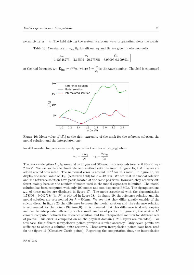
Figure 16: Mean value of |Ez| at the right extremity of the mesh for the reference solution, themodal solution and the interpolated one.
for 401 angular frequencies ω evenly spaced in the interval [ω1, ω2] where
ω1 =2πc0λ1
, ω2 =2πc0λ2
.
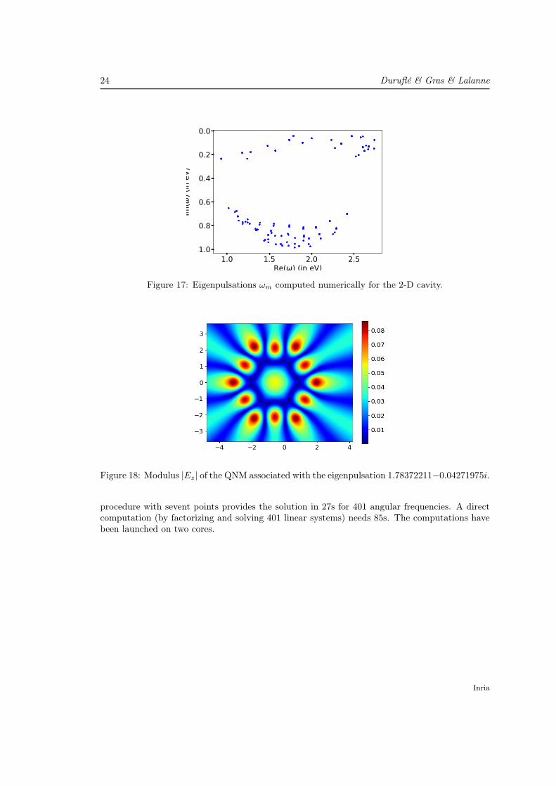
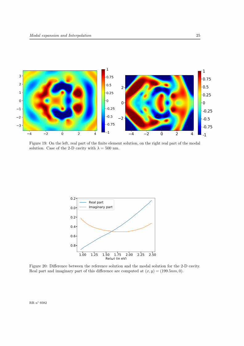
The two wavelengthes λ1, λ2 are equal to 1.3 µm and 500 nm. It corresponds to ω1 ≈ 0.954eV, ω2 ≈2.48eV . We use sixth-order finite element method with the mesh of figure 15, PML layers areadded around this mesh. The numerical error is around 10−5 for this mesh. In figure 16, wedisplay the mean value of |Ez| (scattered field) for x = 420nm. We see that the modal solutionand the reference solution have peaks located at the same positions. However, they are very dif-ferent mainly because the number of modes used in the modal expansion is limited. The modalsolution has been computed with only 100 modes and non-dispersive PMLs. The eigenpulsationsωm of these modes are displayed in figure 17. The mode associated with the eigenpulsation1.78366− 0.042718i (in eV) is plotted in figure 18. In figure 19, the reference solution and themodal solution are represented for λ =500nm. We see that they differ greatly outside of thesilicon discs. In figure 20 the difference between the modal solution and the reference solutionis represented for the point (199.5nm, 0). It is observed that this difference is slowly varyingand can be interpolated efficiently with a small number of points. In figure 21, the relative L2
error is computed between the reference solution and the interpolated solution for different setsof points. This error is computed on all the physical domain (PML layers are excluded). Forthis case, the different interpolation points provide a similar accuracy. Only seven points aresufficient to obtain a solution quite accurate. These seven interpolation points have been usedfor the figure 16 (Clenshaw-Curtis points). Regarding the computation time, the interpolation
RR n° 9382
24 Duruflé & Gras & Lalanne
1.0 1.5 2.0 2.5Re(ω) (in eV)
−1.0
−0.8
−0.6
−0.4
−0.2
0.0
Im(ω
) (in eV)
Figure 17: Eigenpulsations ωm computed numerically for the 2-D cavity.
Figure 18: Modulus |Ez| of the QNM associated with the eigenpulsation 1.78372211−0.04271975i.
procedure with sevent points provides the solution in 27s for 401 angular frequencies. A directcomputation (by factorizing and solving 401 linear systems) needs 85s. The computations havebeen launched on two cores.
Inria
Modal expansion and Interpolation 25
Figure 19: On the left, real part of the finite element solution, on the right real part of the modalsolution. Case of the 2-D cavity with λ = 500 nm.
1.00 1.25 1.50 1.75 2.00 2.25 2.50Re(ω) (in eV)
−0.8
−0.6
−0.4
−0.2
0.0
0.2Real partImaginary part
Figure 20: Difference between the reference solution and the modal solution for the 2-D cavity.Real part and imaginary part of this difference are computed at (x, y) = (199.5nm, 0).
RR n° 9382

26 Duruflé & Gras & Lalanne
5 10 15 20 25Number of points
10 10
10 8
10 6
10 4
10 2
100
Relative error
Clenshaw-Curtis pointsChebyshev pointsLeja points
Figure 21: Relative L2 error between the reference solution and the interpolation solution versusthe number of interpolation points. Case of the 2-D cavity.
Inria
Modal expansion and Interpolation 27
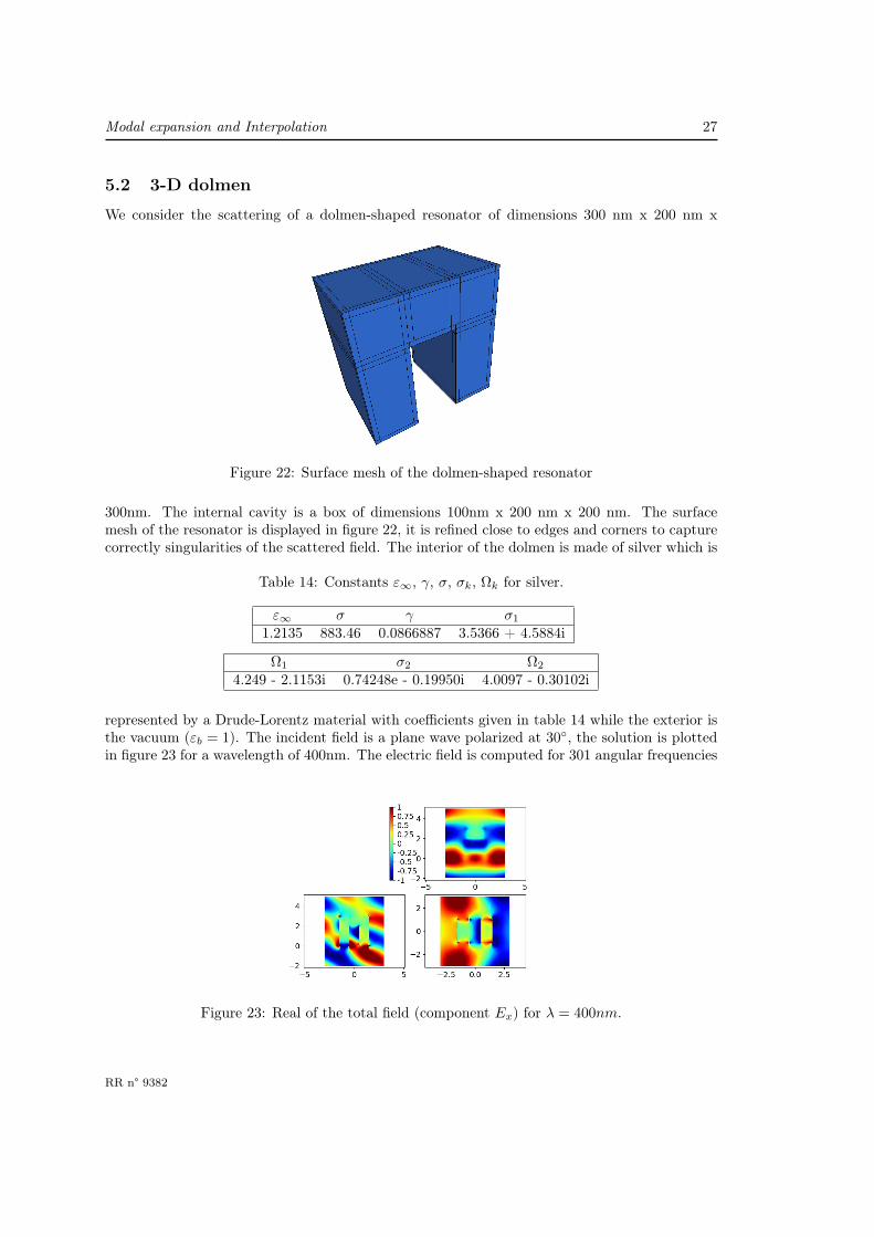
5.2 3-D dolmen
We consider the scattering of a dolmen-shaped resonator of dimensions 300 nm x 200 nm x
Figure 22: Surface mesh of the dolmen-shaped resonator
300nm. The internal cavity is a box of dimensions 100nm x 200 nm x 200 nm. The surfacemesh of the resonator is displayed in figure 22, it is refined close to edges and corners to capturecorrectly singularities of the scattered field. The interior of the dolmen is made of silver which is
Table 14: Constants ε∞, γ, σ, σk, Ωk for silver.
ε∞ σ γ σ1
1.2135 883.46 0.0866887 3.5366 + 4.5884i
Ω1 σ2 Ω2
4.249 - 2.1153i 0.74248e - 0.19950i 4.0097 - 0.30102i
represented by a Drude-Lorentz material with coefficients given in table 14 while the exterior isthe vacuum (εb = 1). The incident field is a plane wave polarized at 30, the solution is plottedin figure 23 for a wavelength of 400nm. The electric field is computed for 301 angular frequencies
Figure 23: Real of the total field (component Ex) for λ = 400nm.
RR n° 9382
28 Duruflé & Gras & Lalanne
ω evenly spaced in the interval [ω1, ω2] where
ω1 =2πc0λ1
, ω2 =2πc0λ2
.
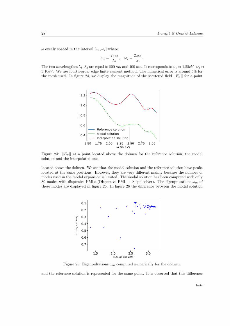
The two wavelengthes λ1, λ2 are equal to 800 nm and 400 nm. It corresponds to ω1 ≈ 1.55eV, ω2 ≈3.10eV . We use fourth-order edge finite element method. The numerical error is around 5% forthe mesh used. In figure 24, we display the magnitude of the scattered field ||ES || for a point
Figure 24: ||ES || at a point located above the dolmen for the reference solution, the modalsolution and the interpolated one.
located above the dolmen. We see that the modal solution and the reference solution have peakslocated at the same positions. However, they are very different mainly because the number ofmodes used in the modal expansion is limited. The modal solution has been computed with only80 modes with dispersive PMLs (Dispersive PML + Slepc solver). The eigenpulsations ωm ofthese modes are displayed in figure 25. In figure 26 the difference between the modal solution
1.5 2.0 2.5 3.0Re(ω) (in eV)
−0.7
−0.6
−0.5
−0.4
−0.3
−0.2
−0.1
Im(ω
) (in eV)
Figure 25: Eigenpulsations ωm computed numerically for the dolmen.
and the reference solution is represented for the same point. It is observed that this difference
Inria
Modal expansion and Interpolation 29
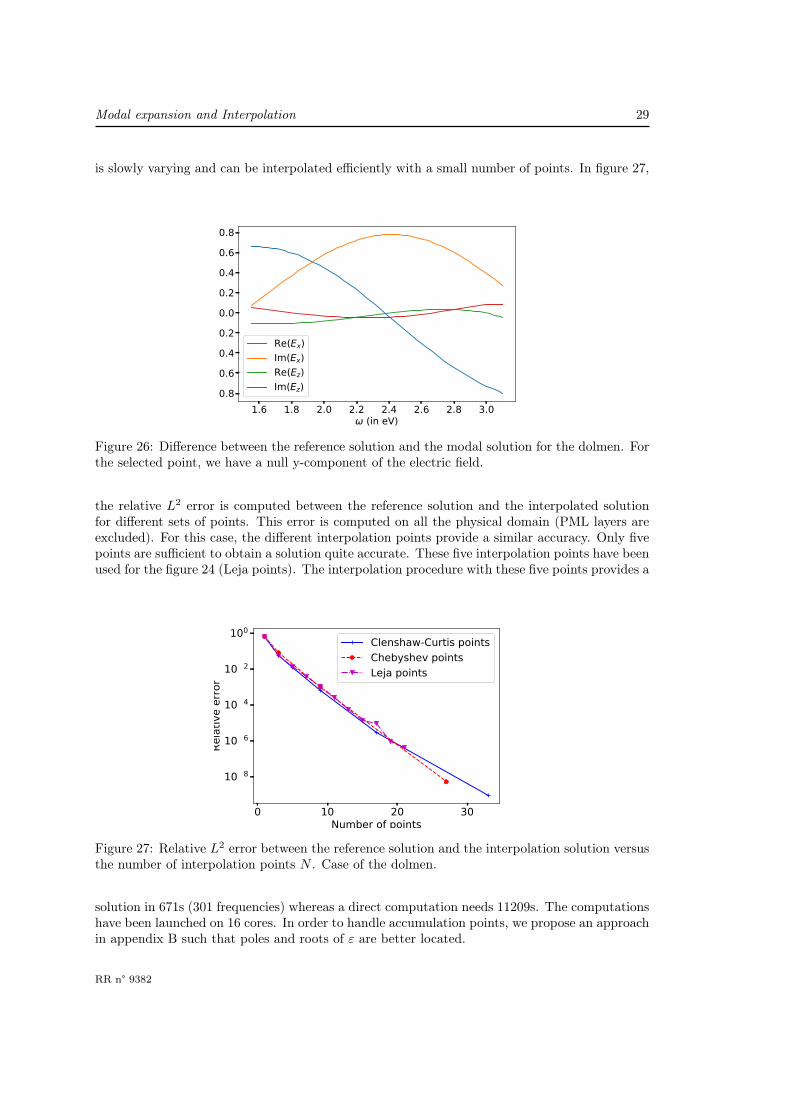
is slowly varying and can be interpolated efficiently with a small number of points. In figure 27,
1.6 1.8 2.0 2.2 2.4 2.6 2.8 3.0ω (in eV)
−0.8−0.6−0.4−0.20.00.20.40.60.8
Re(Ex)Im(Ex)Re(Ez)Im(Ez)
Figure 26: Difference between the reference solution and the modal solution for the dolmen. Forthe selected point, we have a null y-component of the electric field.
the relative L2 error is computed between the reference solution and the interpolated solutionfor different sets of points. This error is computed on all the physical domain (PML layers areexcluded). For this case, the different interpolation points provide a similar accuracy. Only fivepoints are sufficient to obtain a solution quite accurate. These five interpolation points have beenused for the figure 24 (Leja points). The interpolation procedure with these five points provides a
0 10 20 30Number of points
10 8
10 6
10 4
10 2
100
Relative error
Clenshaw-Curtis pointsChebyshev pointsLeja points
Figure 27: Relative L2 error between the reference solution and the interpolation solution versusthe number of interpolation points N . Case of the dolmen.
solution in 671s (301 frequencies) whereas a direct computation needs 11209s. The computationshave been launched on 16 cores. In order to handle accumulation points, we propose an approachin appendix B such that poles and roots of ε are better located.
RR n° 9382
30 Duruflé & Gras & Lalanne
6 Conclusion
In section 3, we have detailed and illustrated the drawbacks of reconstructing the solution on agiven interval [ω1, ω2] by using the eigenmodes of the optical device. Because of these drawbacks,the reconstruction is often inefficient in comparison to a direct computation. We have proposedin section 5 an interpolation procedure to overcome these limitations. This strategy is based onthe interpolation of the difference between the modal solution and the finite element solution.If eigenmodes close to the interval [ω1, ω2] on the real axis are included, this difference is slowlyvarying and can be interpolated efficiently with a few number of points. By using a nestedsequence of interpolation points such as Leja points, we can stop the computation as soon as thesolution is accurate enough. With this approach, we obtain the following nice properties thatsolve the limitations listed in paragraph 3.3:
• Accuracy : the accuracy can be quickly improved by adding a few interpolation points. Weno longer need to include a very large number of modes in order to improve the accuracy.
• Robustness : the convergence is fast and almost does not depend on the source term J. Theconvergence depends mainly on the set of eigenpulsations included in the modal expansion.
• Control : we can reach a given accuracy by increasing the number of interpolation points.
• Accuracy outside the resonator : the accuracy is very good outside the resonator, we donot need to include a larger number of PML modes.
• Eigenvalues in a limited region of the complex plane : Only eigenvalues close to the interval[ω1, ω2] on the real axis are needed.
• Accumulation points : the interpolation procedure itself does not solve this issue. Sincethe permittivity is not null, neither infinite, nor equal to -1 (except for metamaterials) onthe real axis, it seems possible to obtain an analytic approximation of ε(ω) such that polesand zeros are far enough from the real axis. In appendix B, an attempt is made in orderto take these accumulation points away from the real axis.
• Independence from the chosen formula for αm : the convergence is similar with the differentformulas for αm (e.g. formulas (7), (8)). Moreover, the electric field can be reconstructedin 3-D directly with these formulas without the necessity of including static modes.
Finally numerical results presented in section 5 and in appendix A show that the interpolationprocedure is computationally efficient.
References
Amestoy, P., Duff, I., Koster, J., and L’Excellent, J.-Y. (2001). A fully asynchronous multi-frontal solver using distributed dynamic scheduling. SIAM Journal on Matrix Analysis andApplications, 23:15–41.
Binkowski, F., Zschiedrich, L., and Burger, S. (2019). An auxiliary field approach for computingoptical resonances in dispersive media. J. Eur. Opt. Soc.-Rapid Publ.
Campos, C. and Roman, J. E. (2016). Parallel Krylov solvers for the polynomial eigenvalueproblem in SLEPc. SIAM Journal on Scientific Computing, 38(5):385–411.
Inria
Modal expansion and Interpolation 31
Cohen, G. and Duruflé, M. (2007). Non spurious spectral-like element methods for Maxwell’sequations. Journal of Computational Mathematics, 25:282–304.
Colom, R., Mcphedran, R., Stout, B., and Bonod, N. (2018). Modal expansion of the scatteredfield: Causality, nondivergence, and nonresonant contribution. Physical Review B : Condensedmatter and materials physics, 98:085418.
Demésy, G., Nicolet, A., Gralak, B., Geuzaine, C., Campos, C., and Roman, J. E. (2020). Non-linear eigenvalue problems with GetDP and SLEPc: Eigenmode computations of frequency-dispersive photonic open structures. Computer Physics Communications, 257:107509.
Duruflé, M., Gras, A., and Lalanne, P. (2020). Non-uniqueness of the quasinormal mode expan-sion of electromagnetic Lorentz dispersive materials. Technical Report RR-9348, INRIA.
Lalanne, P., Yan, W., Gras, A., Sauvan, C., Hugonin, J.-P., Besbes, M., Demésy, G., Truong,M. D., Gralak, B., Zolla, F., Nicolet, A., Binkowski, F., Zschiedrich, L., Burger, S., Zimmerling,J., Remis, R., Urbach, P., Liu, H. T., and Weiss, T. (2019). Quasinormal mode solvers forresonators with dispersive materials. J. Opt. Soc. Am. A, 36(4):686–704.
Lalanne, P., Yan, W., Vynck, K., Sauvan, C., and Hugonin, J.-P. (2018). Light interaction withphotonic and plasmonic resonances. Laser & Photonics Reviews, page 1700113.
N’diaye, M. (2017). On the study and development of high-order time integration schemesfor ODEs applied to acoustic and electromagnetic wave propagation problems. PhD thesis,Université de Pau et des Pays de l’Adour.
P. Jantsch, C.G. Webster, G. Z. (2016). On the Lebesgue constant of weighted Leja points forLagrange interpolation on unbounded domains. arXiv:1606.07093.
Sehmi, H. S., Langbein, W., and Muljarov, E. A. (2017). Optimizing the Drude-Lorentz modelfor material permittivity: Method, program, and examples for gold, silver, and copper. Phys.Rev. B, 95:115444.
Vial, B., Zolla, F., Nicolet, A., and Commandré, M. (2014). Quasimodal expansion of electro-magnetic fields in open two-dimensional structures. Phys. Rev. A, 89:023829.
Yan, W., Faggiani, R., and Lalanne, P. (2018). Rigorous modal analysis of plasmonic nanores-onators. Phys. Rev. B, 97:205422.
Zimmerling, J., Wei, L., Urbach, P., and Remis, R. (2016). A Lanczos model-order reductiontechnique to efficiently simulate electromagnetic wave propagation in dispersive media. J.Comput. Phys., 315:348–362.
Zschiedrich, L., Binkowski, F., Nikolay, N., Benson, O., Kewes, G., and Burger, S. (2018). Riesz-projection-based theory of light-matter interaction in dispersive nanoresonators. Phys. Rev.A, 98:043806.
RR n° 9382
32 Duruflé & Gras & Lalanne
A Efficiency of interpolation on other cases
In this section, we show the efficiency of the interpolation procedure to reconstruct the field forcases that have been presented in the section 3. The interpolation procedure is described insection 5. Non-dispersive PMLs are used with polynomial eigenvalue solver (PEP) proposed inSlepc. This choice is the most efficient as described in section 4.
A.1 2-D cobra cavity
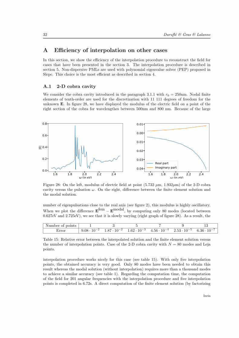
We consider the cobra cavity introduced in the paragraph 3.1.1 with r0 = 250nm. Nodal finiteelements of tenth-order are used for the discretization with 11 111 degrees of freedom for theunknown E. In figure 28, we have displayed the modulus of the electric field on a point of theright section of the cobra for wavelengthes between 500nm and 800 nm. Because of the large
1.6 1.8 2.0 2.2 2.4ω (in eV)
0.0
0.2
0.4
0.6
0.8
|E|
1.6 1.8 2.0 2.2 2.4ω (in eV)
−0.04
−0.03
−0.02
−0.01
0.00
0.01
Real partImaginary part
Figure 28: On the left, modulus of electric field at point (5.732 µm, 1.932µm) of the 2-D cobracavity versus the pulsation ω. On the right, difference between the finite element solution andthe modal solution.
number of eigenpulsations close to the real axis (see figure 2), this modulus is highly oscillatory.When we plot the difference Efem − Emodal, by computing only 80 modes (located between0.627eV and 2.725eV), we see that it is slowly varying (right graph of figure 28). As a result, the
Number of points 1 3 5 7 9 13Error 9.08 · 10−2 1.87 · 10−2 1.62 · 10−3 4.56 · 10−4 2.53 · 10−5 6.36 · 10−7
Table 15: Relative error between the interpolated solution and the finite element solution versusthe number of interpolation points. Case of the 2-D cobra cavity with N = 80 modes and Lejapoints.
interpolation procedure works nicely for this case (see table 15). With only five interpolationpoints, the obtained accuracy is very good. Only 80 modes have been needed to obtain thisresult whereas the modal solution (without interpolation) requires more than a thousand modesto achieve a similar accuracy (see table 1). Regarding the computation time, the computationof the field for 201 angular frequencies with the interpolation procedure and five interpolationpoints is completed in 6.72s. A direct computation of the finite element solution (by factorizing
Inria
Modal expansion and Interpolation 33
and solving 201 linear systems) requires 69.1s. The simulations have been launched on a singlecore.
A.2 3-D cobra cavity
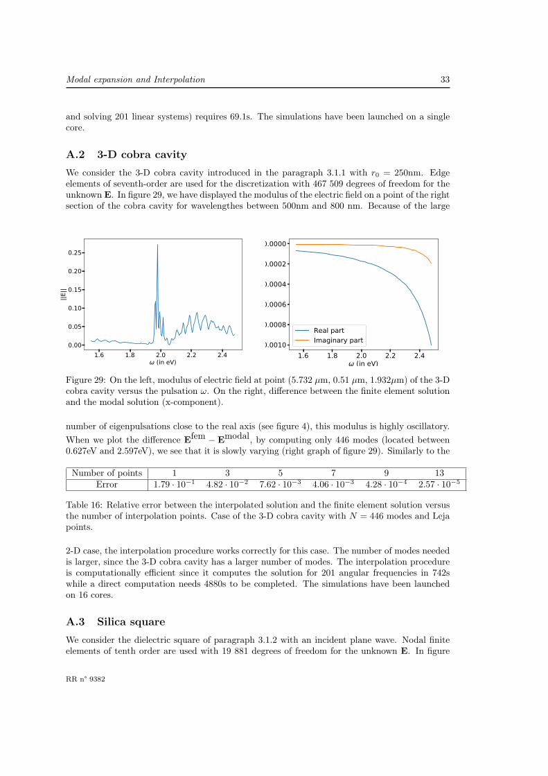
We consider the 3-D cobra cavity introduced in the paragraph 3.1.1 with r0 = 250nm. Edgeelements of seventh-order are used for the discretization with 467 509 degrees of freedom for theunknown E. In figure 29, we have displayed the modulus of the electric field on a point of the rightsection of the cobra cavity for wavelengthes between 500nm and 800 nm. Because of the large
1.6 1.8 2.0 2.2 2.4ω (in eV)
0.00
0.05
0.10
0.15
0.20
0.25
||E||
1.6 1.8 2.0 2.2 2.4ω (in eV)
−0.0010
−0.0008
−0.0006
−0.0004
−0.0002
0.0000
Real partImaginary part
Figure 29: On the left, modulus of electric field at point (5.732 µm, 0.51 µm, 1.932µm) of the 3-Dcobra cavity versus the pulsation ω. On the right, difference between the finite element solutionand the modal solution (x-component).
number of eigenpulsations close to the real axis (see figure 4), this modulus is highly oscillatory.When we plot the difference Efem − Emodal, by computing only 446 modes (located between0.627eV and 2.597eV), we see that it is slowly varying (right graph of figure 29). Similarly to the
Number of points 1 3 5 7 9 13Error 1.79 · 10−1 4.82 · 10−2 7.62 · 10−3 4.06 · 10−3 4.28 · 10−4 2.57 · 10−5
Table 16: Relative error between the interpolated solution and the finite element solution versusthe number of interpolation points. Case of the 3-D cobra cavity with N = 446 modes and Lejapoints.
2-D case, the interpolation procedure works correctly for this case. The number of modes neededis larger, since the 3-D cobra cavity has a larger number of modes. The interpolation procedureis computationally efficient since it computes the solution for 201 angular frequencies in 742swhile a direct computation needs 4880s to be completed. The simulations have been launchedon 16 cores.
A.3 Silica square
We consider the dielectric square of paragraph 3.1.2 with an incident plane wave. Nodal finiteelements of tenth order are used with 19 881 degrees of freedom for the unknown E. In figure
RR n° 9382
34 Duruflé & Gras & Lalanne
0.6 0.7 0.8 0.9 1.0 1.1 1.2ω (in eV)
0.0
0.5
1.0
1.5
2.0
2.5
3.0
||E||
0.6 0.7 0.8 0.9 1.0 1.1 1.2ω (in eV)
−0.2
−0.1
0.0
0.1
0.2
0.3Real partImaginary part
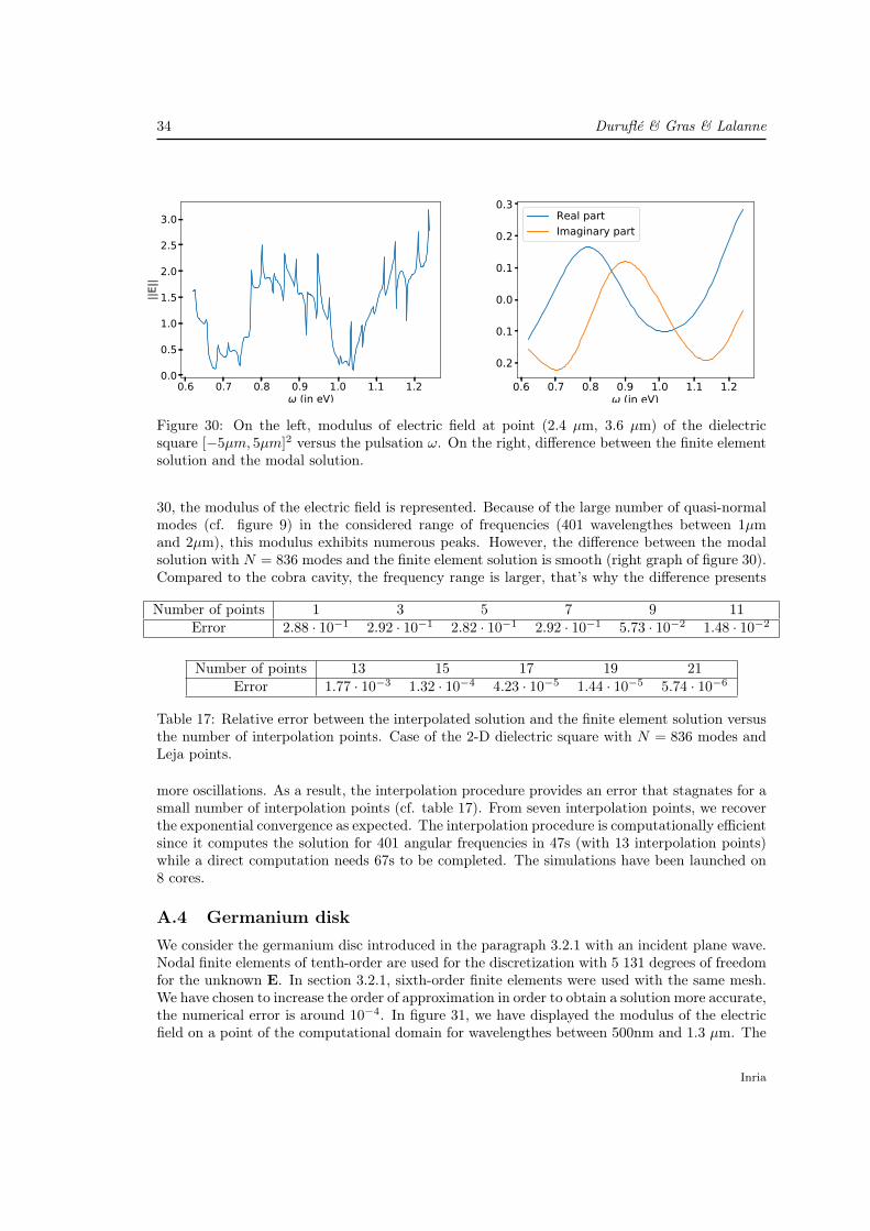
Figure 30: On the left, modulus of electric field at point (2.4 µm, 3.6 µm) of the dielectricsquare [−5µm, 5µm]2 versus the pulsation ω. On the right, difference between the finite elementsolution and the modal solution.
30, the modulus of the electric field is represented. Because of the large number of quasi-normalmodes (cf. figure 9) in the considered range of frequencies (401 wavelengthes between 1µmand 2µm), this modulus exhibits numerous peaks. However, the difference between the modalsolution with N = 836 modes and the finite element solution is smooth (right graph of figure 30).Compared to the cobra cavity, the frequency range is larger, that’s why the difference presents
Number of points 1 3 5 7 9 11Error 2.88 · 10−1 2.92 · 10−1 2.82 · 10−1 2.92 · 10−1 5.73 · 10−2 1.48 · 10−2
Number of points 13 15 17 19 21Error 1.77 · 10−3 1.32 · 10−4 4.23 · 10−5 1.44 · 10−5 5.74 · 10−6
Table 17: Relative error between the interpolated solution and the finite element solution versusthe number of interpolation points. Case of the 2-D dielectric square with N = 836 modes andLeja points.
more oscillations. As a result, the interpolation procedure provides an error that stagnates for asmall number of interpolation points (cf. table 17). From seven interpolation points, we recoverthe exponential convergence as expected. The interpolation procedure is computationally efficientsince it computes the solution for 401 angular frequencies in 47s (with 13 interpolation points)while a direct computation needs 67s to be completed. The simulations have been launched on8 cores.
A.4 Germanium diskWe consider the germanium disc introduced in the paragraph 3.2.1 with an incident plane wave.Nodal finite elements of tenth-order are used for the discretization with 5 131 degrees of freedomfor the unknown E. In section 3.2.1, sixth-order finite elements were used with the same mesh.We have chosen to increase the order of approximation in order to obtain a solution more accurate,the numerical error is around 10−4. In figure 31, we have displayed the modulus of the electricfield on a point of the computational domain for wavelengthes between 500nm and 1.3 µm. The
Inria
Modal expansion and Interpolation 35
1.00 1.25 1.50 1.75 2.00 2.25 2.50ω (in eV)
0.40
0.45
0.50
0.55
0.60
||E||
1.00 1.25 1.50 1.75 2.00 2.25 2.50ω (in eV)
−0.30
−0.25
−0.20
−0.15
−0.10
−0.05
0.00 N=124N=414
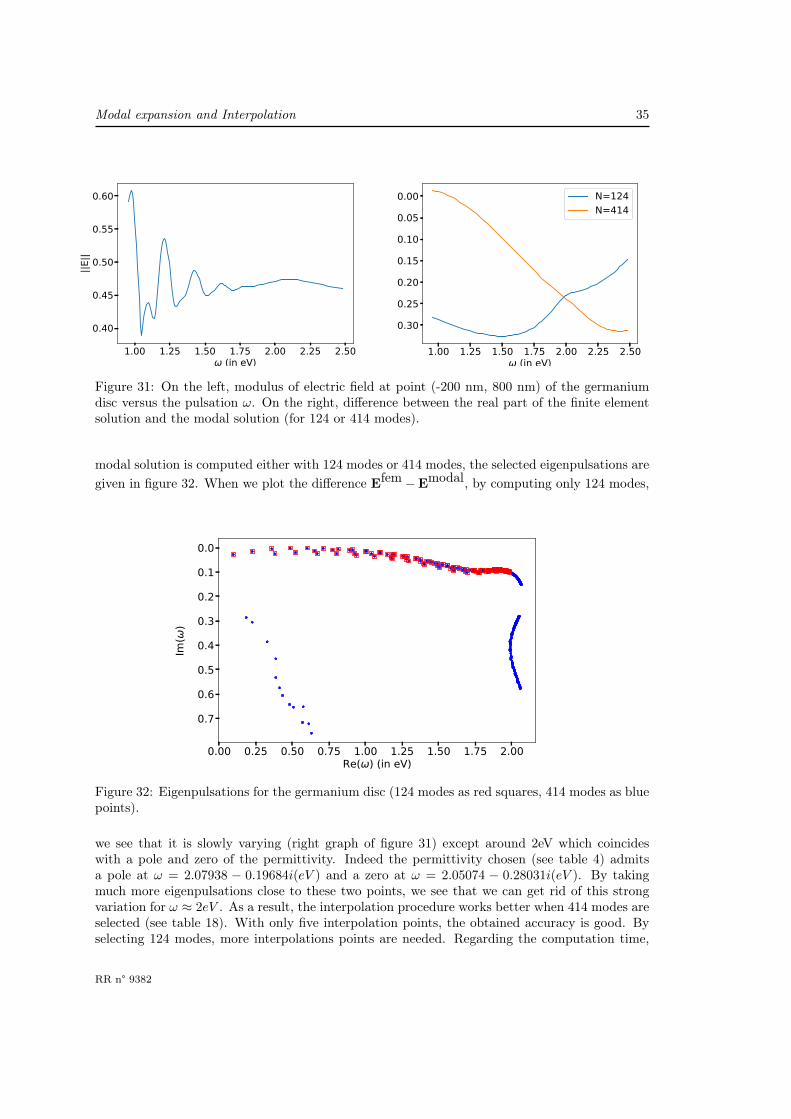
Figure 31: On the left, modulus of electric field at point (-200 nm, 800 nm) of the germaniumdisc versus the pulsation ω. On the right, difference between the real part of the finite elementsolution and the modal solution (for 124 or 414 modes).
modal solution is computed either with 124 modes or 414 modes, the selected eigenpulsations aregiven in figure 32. When we plot the difference Efem −Emodal, by computing only 124 modes,
0.00 0.25 0.50 0.75 1.00 1.25 1.50 1.75 2.00Re(ω) (in eV)
−0.7
−0.6
−0.5
−0.4
−0.3
−0.2
−0.1
0.0
Im(ω
)
Figure 32: Eigenpulsations for the germanium disc (124 modes as red squares, 414 modes as bluepoints).
we see that it is slowly varying (right graph of figure 31) except around 2eV which coincideswith a pole and zero of the permittivity. Indeed the permittivity chosen (see table 4) admitsa pole at ω = 2.07938 − 0.19684i(eV ) and a zero at ω = 2.05074 − 0.28031i(eV ). By takingmuch more eigenpulsations close to these two points, we see that we can get rid of this strongvariation for ω ≈ 2eV . As a result, the interpolation procedure works better when 414 modes areselected (see table 18). With only five interpolation points, the obtained accuracy is good. Byselecting 124 modes, more interpolations points are needed. Regarding the computation time,
RR n° 9382
36 Duruflé & Gras & Lalanne
Number of points 1 3 5 7 9 13Error (N = 124) 4.12 · 10−1 5.73 · 10−2 1.66 · 10−2 1.56 · 10−2 1.03 · 10−2 6.38 · 10−3
Error (N = 414) 3.92 · 10−1 5.06 · 10−2 3.59 · 10−3 2.34 · 10−3 8.34 · 10−4 2.98 · 10−4
Table 18: Relative error between the interpolated solution and the finite element solution versusthe number of interpolation points. Case of the germanium disc with N = 124 modes or N = 414modes and Leja points.
the computation of the field for 201 angular frequencies with the interpolation procedure andfive interpolation points and N = 414 modes is completed in 130s. If we select 13 interpolationpoints and N = 124 modes, the computation is completed in 32s. A direct computation of thefinite element solution (by factorizing and solving 201 linear systems) requires 37.5s. For thiscase, it is more efficient to select a limited number of modes. The simulations have been launchedon a single core.
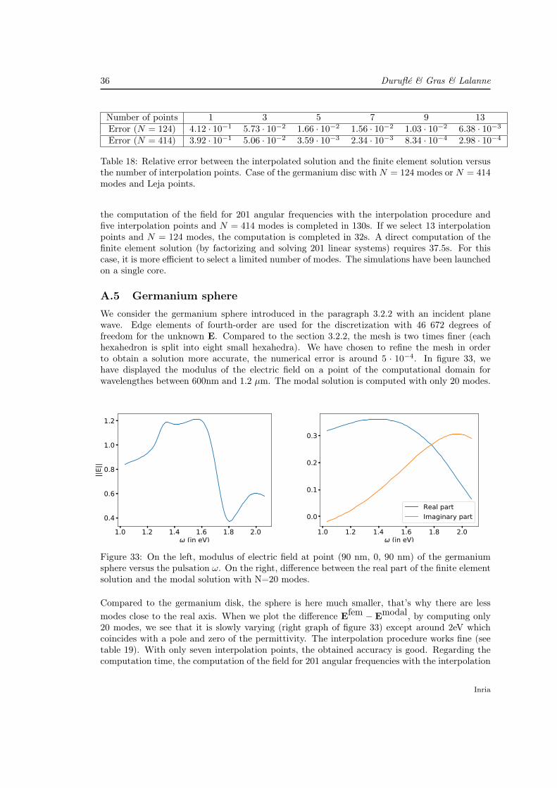
A.5 Germanium sphereWe consider the germanium sphere introduced in the paragraph 3.2.2 with an incident planewave. Edge elements of fourth-order are used for the discretization with 46 672 degrees offreedom for the unknown E. Compared to the section 3.2.2, the mesh is two times finer (eachhexahedron is split into eight small hexahedra). We have chosen to refine the mesh in orderto obtain a solution more accurate, the numerical error is around 5 · 10−4. In figure 33, wehave displayed the modulus of the electric field on a point of the computational domain forwavelengthes between 600nm and 1.2 µm. The modal solution is computed with only 20 modes.
1.0 1.2 1.4 1.6 1.8 2.0ω (in eV)
0.4
0.6
0.8
1.0
1.2
||E||
1.0 1.2 1.4 1.6 1.8 2.0ω (in eV)
0.0
0.1
0.2
0.3
Real partImaginary part
Figure 33: On the left, modulus of electric field at point (90 nm, 0, 90 nm) of the germaniumsphere versus the pulsation ω. On the right, difference between the real part of the finite elementsolution and the modal solution with N=20 modes.
Compared to the germanium disk, the sphere is here much smaller, that’s why there are lessmodes close to the real axis. When we plot the difference Efem − Emodal, by computing only20 modes, we see that it is slowly varying (right graph of figure 33) except around 2eV whichcoincides with a pole and zero of the permittivity. The interpolation procedure works fine (seetable 19). With only seven interpolation points, the obtained accuracy is good. Regarding thecomputation time, the computation of the field for 201 angular frequencies with the interpolation
Inria
Modal expansion and Interpolation 37
Number of points 1 3 5 7 9 13Error 7.81 · 10−1 5.70 · 10−2 8.32 · 10−3 3.18 · 10−3 8.34 · 10−4 9.94 · 10−5
Table 19: Relative error between the interpolated solution and the finite element solution versusthe number of interpolation points. Case of the germanium sphere with N = 20 modes and Lejapoints.
procedure and seven interpolation points is completed in 27s. A direct computation of the finiteelement solution (by factorizing and solving 201 linear systems) requires 218s. The simulationshave been launched on 8 cores.
B Displacement of roots and poles of the permittivity func-tion
In this section, we propose a strategy in order to avoid the proximity of poles or zeros of ε(ω)to the real axis. Indeed, if the poles or roots of ε(ω) are close to the real axis, we have seen insection 3 that it will increase the number of modes required to obtain an accurate modal solution.It is an also an issue if the interpolation procedure described in 5 is used because the eigensolvermay fail to compute the eigenpulsations close to the interval [ω1, ω2] on the real axis because ofaccumulation of eigenpulsations on roots or poles of ε(ω). The number of modes close to theinterval [ω1, ω2] can also be very large. In order to control the position of the poles or roots, wesearch ε with the following expression
ε(ω) = ε∞(ω −R1)(ω + R1) · · · (ω −Rn)(ω + Rn)
(ω − Ω1)(ω + Ω1) · · · (ω − Ωn)(ω + Ωn)(15)
where Ri are roots of ε(ω) and Ωi poles of ε. If Ωi is a pole, we impose that −Ωi is also apole and similarly for roots. With this approach, the permittivity given by equation (15) iscausal. The parameters ε∞, R1, R2, · · · , Rn,Ω1,Ω2, · · · ,Ωn are searched such that the quantityε(ω) − εmes(ω) is minimized where εmes is the measured permittivity. We can minimize thisquantity under constraints such that
Im(Ri) ≤ −0.5, Im(Ωi) ≤ −0.5 (16)
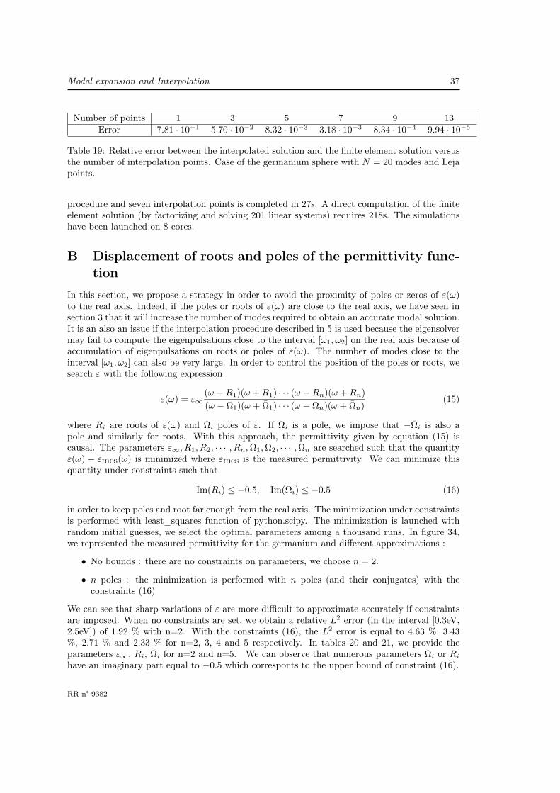
in order to keep poles and root far enough from the real axis. The minimization under constraintsis performed with least_squares function of python.scipy. The minimization is launched withrandom initial guesses, we select the optimal parameters among a thousand runs. In figure 34,we represented the measured permittivity for the germanium and different approximations :
• No bounds : there are no constraints on parameters, we choose n = 2.
• n poles : the minimization is performed with n poles (and their conjugates) with theconstraints (16)
We can see that sharp variations of ε are more difficult to approximate accurately if constraintsare imposed. When no constraints are set, we obtain a relative L2 error (in the interval [0.3eV,2.5eV]) of 1.92 % with n=2. With the constraints (16), the L2 error is equal to 4.63 %, 3.43%, 2.71 % and 2.33 % for n=2, 3, 4 and 5 respectively. In tables 20 and 21, we provide theparameters ε∞, Ri, Ωi for n=2 and n=5. We can observe that numerous parameters Ωi or Rihave an imaginary part equal to −0.5 which corresponts to the upper bound of constraint (16).
RR n° 9382
38 Duruflé & Gras & Lalanne
0.5 1.0 1.5 2.0 2.5ω (in eV)
5
10
15
20
25
30
Re(ε)
Measured εNo bounds2 poles3 poles4 poles
0.5 1.0 1.5 2.0 2.5ω (in eV)
0
5
10
15
20
25
30
Im(ε)
Measured εNo bounds2 poles3 poles4 poles
Figure 34: On the left real part of ε(ω), on the right imaginary part (germanium). We showthe measured permittivity, the obtained permittivity when no bounds are prescribed for theparameters (i.e. no constraints), and the permittivity obtained by constraining the parameterswith n=2, 3, 4.
ε∞ Re(R1) Im(R1) Re(Ω1) Im(Ω1)5.50488573 3.52354416 -2.12375772 2.07954764 -0.5
Re(R2) Im(R2) Re(Ω2) Im(Ω2)1.74885098 -0.5 1.87010153 -0.69106174
Table 20: Parameters for the germanium with Im(Ri) ≤ −0.5, Im(Ωi) ≤ −0.5 and n=2.
ε∞ Re(R1) Im(R1) Re(Ω1) Im(Ω1) Re(R2) Im(R2)2.45352827 2.48266876 -0.55333114 1.6010841 -0.50349749 5.88696178 -3.59561585
Re(Ω2) Im(Ω2) Re(R3) Im(R3) Re(Ω3) Im(Ω3) Re(R4)2.15350011 -0.5 2.46992867 -0.50000008 2.15262651 -0.50000002 1.76296625
Im(R4) Re(Ω4) Im(Ω4) Re(R5) Im(R5) Re(Ω5) Im(Ω4)-0.5 3.14808755 -0.50115937 1.76296605 -0.50000005 2.15152138 -0.5
Table 21: Parameters for the germanium with Im(Ri) ≤ −0.5, Im(Ωi) ≤ −0.5 and n=5.
Inria
RESEARCH CENTREBORDEAUX – SUD-OUEST
200 avenue de la Vieille Tour33405 Talence Cedex
PublisherInriaDomaine de Voluceau - RocquencourtBP 105 - 78153 Le Chesnay Cedexinria.fr
ISSN 0249-6399