Improvements in Curved Mesh Adaptation Procedure for the

Omega3P Code

Gerrett Diamonda, Morteza H. Sibonia, Cameron W. Smitha, Mark S. Shepharda,∗

aScientific Computation Research Center, Rensselaer Polytechnic Institute,Troy, NY 12180

1. Introduction

In this report, we provide some details on the state of the Omega3P project. In particular,

Sec. 2 provides the details of in-memory mesh integration. Section 3 describes what has been

done for partitioning and load balancing. In Sec. 4 we discuss the details of the adaptive

loop implementation and provide some example results. Finally, Sec. 5 provides a quick

overview of the steps taken towards moving to higher-order geometric meshes.

2. Fully Parallel In-Memory Mesh Integration

In order to achieve high performing and scalable component interactions between Omega3P

and PUMI we avoid any serial steps and file-based I/O through in-memory data streams

and component functional interfaces. Towards complete support of the solve-adapt cycle we

have implemented in-memory procedures to convert Omega3P meshes and fields to and from

PUMI data structures. The key advantage of this approach is that a small amount of code

is required; we read and write the Omega3P mesh and field structures by directly accessing

PUMI data structures. A similar PUMI in-memory integration with the Albany Multiphysics

framework [1, 11] reduced the data transfer time required to support an adaptive step on a

22 million element mesh from over 100 seconds using files to 23 seconds on 1024 cores.

∗Corresponding authorEmail addresses: diamog@rpi.edu (Gerrett Diamond), hakimm2@rpi.edu (Morteza H. Siboni),

smithc11@rpi.edu (Cameron W. Smith), shephard@rpi.edu (Mark S. Shephard )

Report August 19, 2016

Mesh conversion begins with a version of Omega3P’s NetCDF file reader that is altered to

read the mesh data into PUMI data structures instead of Omega3P’s Distmesh. With the

PUMI mesh we are able to perform partitioning and load balancing as well as adaptation

while only storing the PUMI mesh. After we have a finalized PUMI mesh a second overloaded

version of Omega3P’s file reader is used to convert the PUMI mesh to Omega3P’s Distmesh.

This is done by using the data from the in-memory PUMI mesh as the input instead of

the NetCDF file. After the conversion to Distmesh, we store both the PUMI Mesh and

the Omega3P Distmesh for the duration of the finite element setup and computations. The

time required to convert from the parallel PUMI mesh to the parallel Distmesh is less than

0.1% of the total execution time. The adaptive loop calls the PUMI-to-Distmesh conversion

routines every solve-adapt cycle after executing PUMI mesh adaptation and load balancing

(see further below for more details). We have demonstrated a low runtime and memory

overhead implementation for the PUMI-to-Distmesh conversion which ensures that it is not

a bottleneck in these simulations.

2.1. Results

The “cost” of our in-memory integration approach is an increase in peak memory usage

during the data transfer when there are two copies of the mesh and/or field data stored in

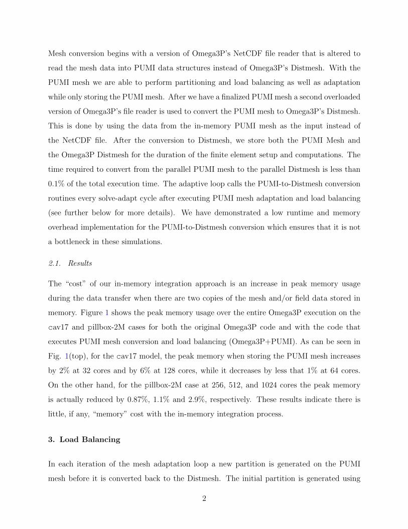
memory. Figure 1 shows the peak memory usage over the entire Omega3P execution on the

cav17 and pillbox-2M cases for both the original Omega3P code and with the code that

executes PUMI mesh conversion and load balancing (Omega3P+PUMI). As can be seen in

Fig. 1(top), for the cav17 model, the peak memory when storing the PUMI mesh increases

by 2% at 32 cores and by 6% at 128 cores, while it decreases by less that 1% at 64 cores.

On the other hand, for the pillbox-2M case at 256, 512, and 1024 cores the peak memory

is actually reduced by 0.87%, 1.1% and 2.9%, respectively. These results indicate there is

little, if any, “memory” cost with the in-memory integration process.

3. Load Balancing

In each iteration of the mesh adaptation loop a new partition is generated on the PUMI

mesh before it is converted back to the Distmesh. The initial partition is generated using

2

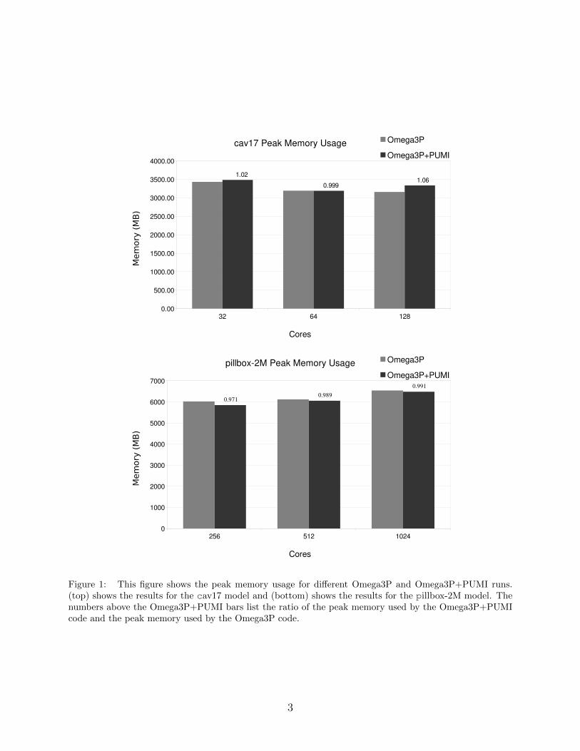
Figure 1: This figure shows the peak memory usage for different Omega3P and Omega3P+PUMI runs.(top) shows the results for the cav17 model and (bottom) shows the results for the pillbox-2M model. Thenumbers above the Omega3P+PUMI bars list the ratio of the peak memory used by the Omega3P+PUMIcode and the peak memory used by the Omega3P code.

3

Zoltan’s graph partitioning. Then SCOREC’s ParMA partitioning tool, which used mesh

adjacencies, is used to perform load balancing by iterative diffusion. ParMA’s multi-entity

balancing traverses an application-specified priority list of entity orders (vertex, edge, face,

region) to balance in descending orders. For each entity order, iterative diffusion steps are

executed until balance is reached or no further improvement is possible.

ParMA’s support for multi-entity balancing was extended for Omega3P’s needs. The Omega3P

solving step relies on both on-part (or local) mesh entities as well as a layer of ghosted (or

remote) elements along each part boundary. Omega3P’s ghosting uses vertex adjacency such

that every element that shares a vertex with a part boundary will be ghosted to each part

that shares that boundary. Figure 2 shows an example of a mesh with a layer of ghosted

elements. In order to improve Omega3P’s performance and scalability, ParMA targets min-

imizing the sum of the ghosted and on-part elements as well as the mesh entities holding

degrees-of-freedom.

Figure 2: A layer of ghosted elements from part A to part B. The darker elements represent all the elementson part A that part B will copy to create its remote mesh.

ParMA balances the degree-of-freedom holders defined by hierarchical Nedelec basis func-

tions [4, 5] by reusing existing multi-entity target and boundary-element selection procedures.

For linear elements this requires balancing edges. For quadratic elements, on the other hand,

this requires edges and faces. For higher than quadratic elements, edges, faces, and regions

4

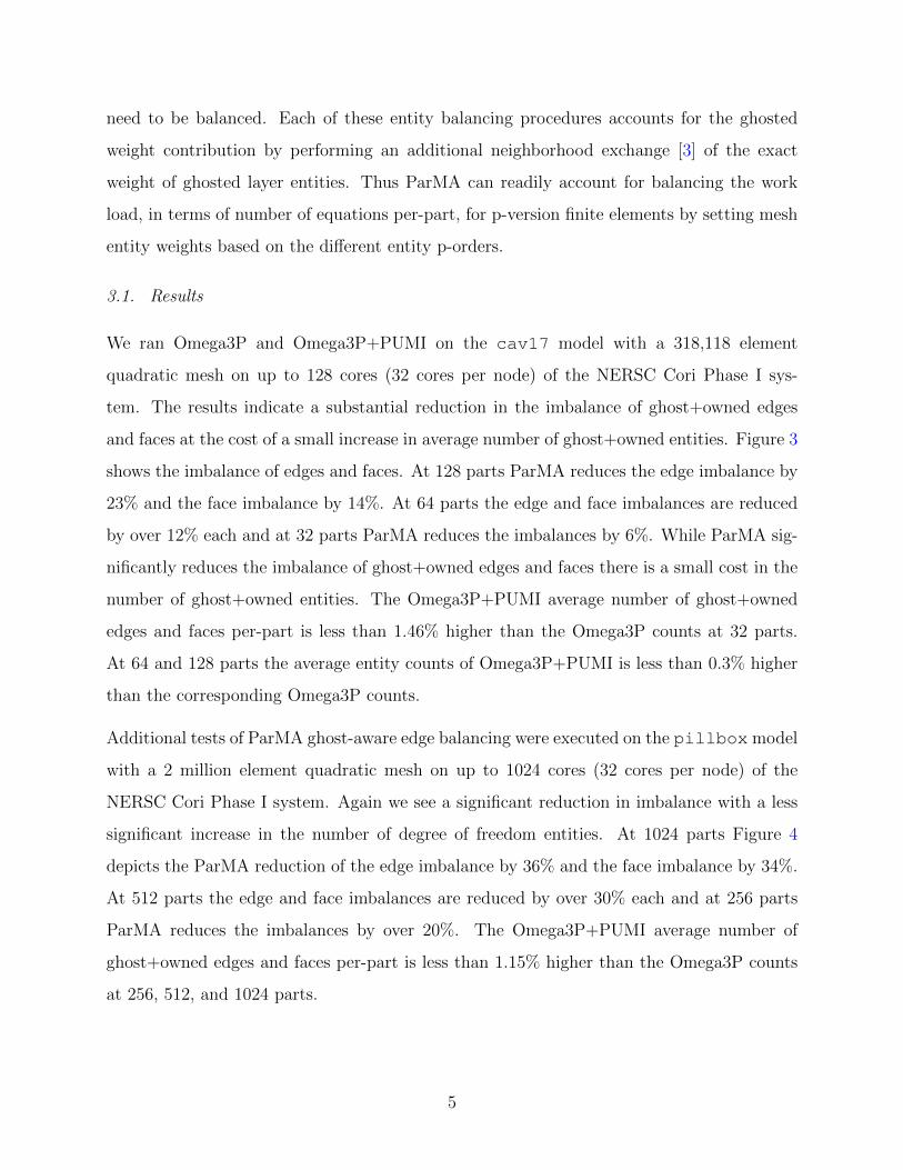
need to be balanced. Each of these entity balancing procedures accounts for the ghosted

weight contribution by performing an additional neighborhood exchange [3] of the exact

weight of ghosted layer entities. Thus ParMA can readily account for balancing the work

load, in terms of number of equations per-part, for p-version finite elements by setting mesh

entity weights based on the different entity p-orders.

3.1. Results

We ran Omega3P and Omega3P+PUMI on the cav17 model with a 318,118 element

quadratic mesh on up to 128 cores (32 cores per node) of the NERSC Cori Phase I sys-

tem. The results indicate a substantial reduction in the imbalance of ghost+owned edges

and faces at the cost of a small increase in average number of ghost+owned entities. Figure 3

shows the imbalance of edges and faces. At 128 parts ParMA reduces the edge imbalance by

23% and the face imbalance by 14%. At 64 parts the edge and face imbalances are reduced

by over 12% each and at 32 parts ParMA reduces the imbalances by 6%. While ParMA sig-

nificantly reduces the imbalance of ghost+owned edges and faces there is a small cost in the

number of ghost+owned entities. The Omega3P+PUMI average number of ghost+owned

edges and faces per-part is less than 1.46% higher than the Omega3P counts at 32 parts.

At 64 and 128 parts the average entity counts of Omega3P+PUMI is less than 0.3% higher

than the corresponding Omega3P counts.

Additional tests of ParMA ghost-aware edge balancing were executed on the pillbox model

with a 2 million element quadratic mesh on up to 1024 cores (32 cores per node) of the

NERSC Cori Phase I system. Again we see a significant reduction in imbalance with a less

significant increase in the number of degree of freedom entities. At 1024 parts Figure 4

depicts the ParMA reduction of the edge imbalance by 36% and the face imbalance by 34%.

At 512 parts the edge and face imbalances are reduced by over 30% each and at 256 parts

ParMA reduces the imbalances by over 20%. The Omega3P+PUMI average number of

ghost+owned edges and faces per-part is less than 1.15% higher than the Omega3P counts

at 256, 512, and 1024 parts.

5

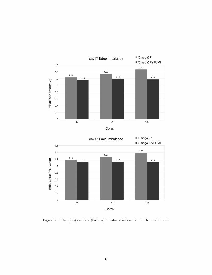
Figure 3: Edge (top) and face (bottom) imbalance information in the cav17 mesh.

6

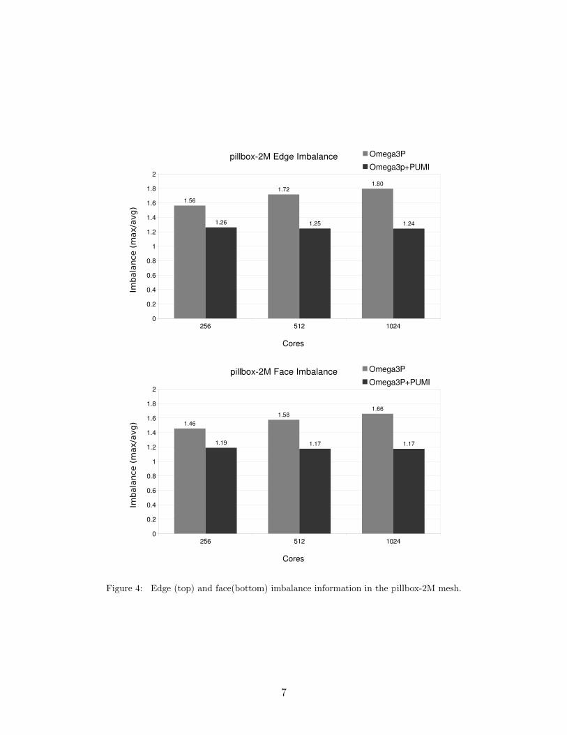
Figure 4: Edge (top) and face(bottom) imbalance information in the pillbox-2M mesh.

7

3.2. Future Steps

While we have seen major improvements in the degree of freedom holder imbalance, we

have yet to see an improvement in runtime as a result of the balancing. It has been shown

that these reductions to the degree-of-freedom holding entities significantly improve the

performance and scalability of parallel finite element simulations [12]. Thus our plan for

future developments in regard to the load balancing is as follows:

• Determine how the distribution of degrees of freedom effects the runtime for Omega3P.

• Further optimize the ParMA ghost balancer to improve runtime of Omega3P solvers.

4. The Adaptive Loop

For the adaptive loop we use a size-driven mesh adaptation procedure [7], in which a mesh

size metric is defined for the desired size of the elements. Then a series of mesh modifications

are applied to achieve the desired edge lengths in the mesh. These operations are:

• Coarsening: This stage removes the edges in the mesh that are shorter than the

desired edge length. This is achieved by applying collapse operations on short edges.

• Refinement: This stage applies edge-based refinement to the mesh in order to achieve

the desired edge-lengths. This stage is accompanied by other local mesh modification

steps to snap the newly created nodes during the refinement step to the model bound-

ary. They are repeated until the desired sizes are achieved.

• Shape improvement: This stage uses operations like edge-swap and vertex reposi-

tioning to improve the quality of the mesh. Currently, not implemented for curved

meshes in PUMI.

A mesh validity check is performed anytime a local mesh modification is run in places with

curved elements to ensure that the resulting elements are not inverted [see 8, for more details].

The pseudo-code for the above-described curve adapt procedure is given below.

With the in-memory integration technique described in section 2, we always have access to

a PUMI mesh object which enables us to seamlessly integrate the Omega3P’s eigen-solvers

8

Algorithm 1 The Curve Adapt

1: procedure CurveAdapt(PumiMesh, SizeField)2: pre-adapt balancing of the mesh3: fix invalid elements4: coarsening5: mid-adapt balancing of the mesh6: refinement and snapping to model boundary7: fix invalid elements8: post-adapt balancing of the mesh9: shape improvement[currently not implemented for curved meshes]

with different PUMI functionalities, such as load-balancing which was discussed earlier in

this report, and adaptations. The following pseudo-code shows the implemented adaptive

loop which make use of Omega3P’s eigen-solver to compute a size field which is then input

in the curve adapt procedure described above.

Algorithm 2 The Adaptive Loop

1: while not converged2: partition the mesh using ParMA with a focus of owned and ghost elements3: convert PUMI mesh to Distmesh4: run the appropriate Omega3P eigensolver5: transfer electric field values to the PUMI mesh6: check for convergence7: run Super-convergent Patch Recovery (SPR) error estimator to obtain the size field8: run CurveAdapt

Note that our current pipeline works with PUMI meshes as an input without the need for an

input NetCDF mesh. This enables us to generate our initial meshes using Simmetrix. The

geometric model inquiries for the purpose of snapping the vertex and mid-edge nodes to the

model are then fully and reliably supported by Simmetrix geometry interrogation API.

Also worth mentioning, is the fact that our current adaptive loop improves upon the previ-

ously available adaptive loop (implemented by Kai) in that each, and every, step is executed

in parallel within the in-memory process. The previous implementation required repartition-

ing a serial mesh after parallel adaptation.

9

4.1. Results for the Adaptive Loop

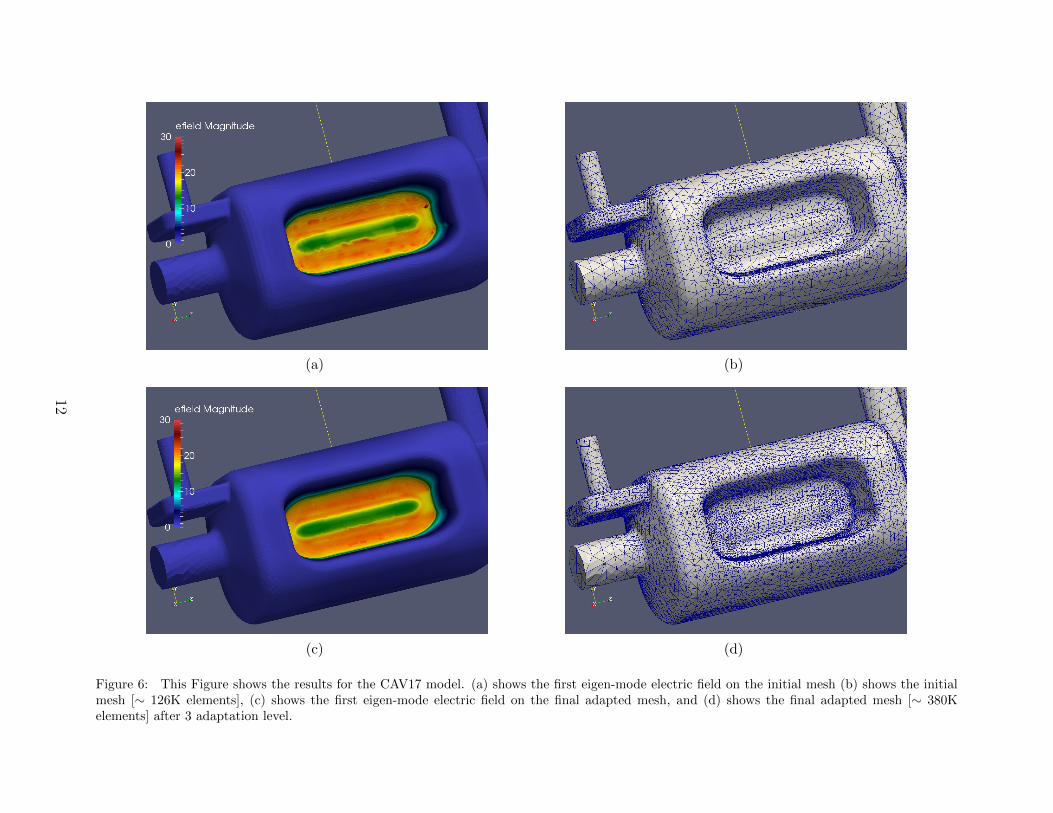
Figures 5 and 6 show two working examples for the current curve adaptation loop. In

particular, Fig. 5 shows the results for the smaller “PILLBOX” model. We start with a

uniform and relatively coarse mesh as shown in Fig. 5(b). The desired size field for this

initial mesh is obtained based on the magnitude of the electric filed shown in Fig. 5(a).

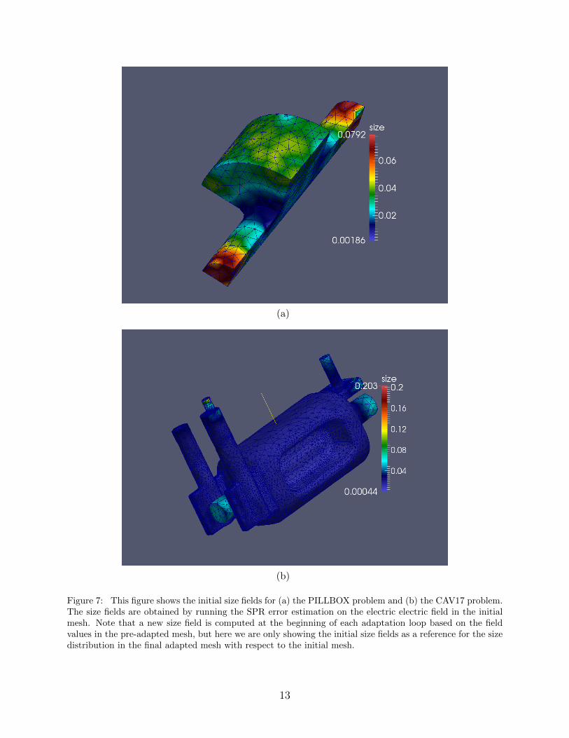
The resulting size field is plotted in Fig. 7(a). The final, adapted mesh (for this specific

example we needed 3 levels of adaptation) and the final electric field for the first eigen-mode

are shown in Figs. 5(d) and 5(c), respectively. Figure 6 shows the corresponding result for

the larger “CAV17” model.

10

(a) (b)

(c) (d)

Figure 5: This Figure shows the results for the PILLBOX model. (a) shows the first eigen-mode electric field on the initial uniform mesh (b) showsthe initial uniform mesh [∼ 3.7K elements], (c) shows the first eigen-mode electric field on the final adapted mesh, and (d) shows the final adaptedmesh [∼ 14K elements] after 3 adaptation level.

11

(a) (b)

(c) (d)

Figure 6: This Figure shows the results for the CAV17 model. (a) shows the first eigen-mode electric field on the initial mesh (b) shows the initialmesh [∼ 126K elements], (c) shows the first eigen-mode electric field on the final adapted mesh, and (d) shows the final adapted mesh [∼ 380Kelements] after 3 adaptation level.

12

(a)

(b)

Figure 7: This figure shows the initial size fields for (a) the PILLBOX problem and (b) the CAV17 problem.The size fields are obtained by running the SPR error estimation on the electric electric field in the initialmesh. Note that a new size field is computed at the beginning of each adaptation loop based on the fieldvalues in the pre-adapted mesh, but here we are only showing the initial size fields as a reference for the sizedistribution in the final adapted mesh with respect to the initial mesh.

13

4.2. Future Steps

Our plan for future developments in regard to the adaptive loop is as follows:

• Work on the shape improvement step in the adaptive loop for curved meshes inorder to be able to produce better quality adapted curved meshes.

• Improve the efficiency of the expensive curved geometry operations.

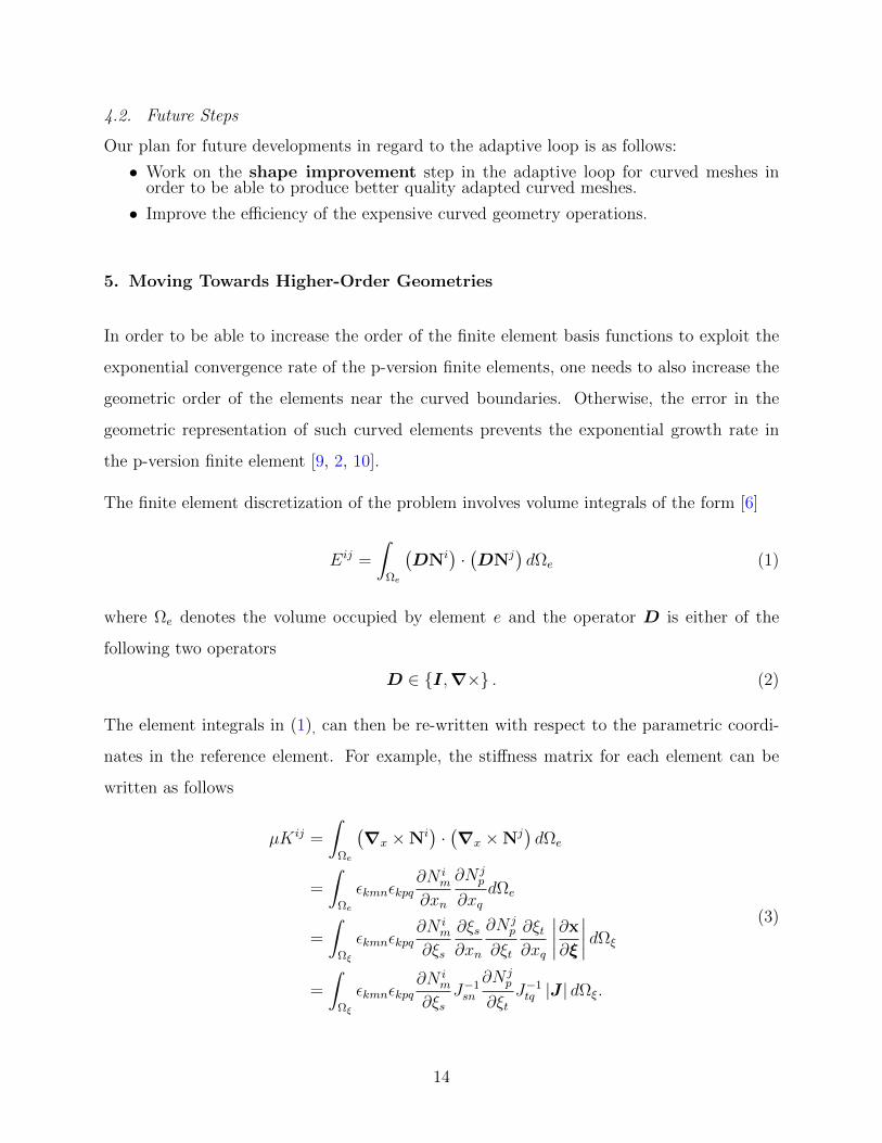
5. Moving Towards Higher-Order Geometries

In order to be able to increase the order of the finite element basis functions to exploit the

exponential convergence rate of the p-version finite elements, one needs to also increase the

geometric order of the elements near the curved boundaries. Otherwise, the error in the

geometric representation of such curved elements prevents the exponential growth rate in

the p-version finite element [9, 2, 10].

The finite element discretization of the problem involves volume integrals of the form [6]

Eij =

∫Ωe

(DNi

)·(DNj

)dΩe (1)

where Ωe denotes the volume occupied by element e and the operator D is either of the

following two operators

D ∈ I,∇× . (2)

The element integrals in (1), can then be re-written with respect to the parametric coordi-

nates in the reference element. For example, the stiffness matrix for each element can be

written as follows

µKij =

∫Ωe

(∇x ×Ni

)·(∇x ×Nj

)dΩe

=

∫Ωe

εkmnεkpq∂N i

m

∂xn

∂N jp

∂xqdΩe

=

∫Ωξ

εkmnεkpq∂N i

m

∂ξs

∂ξs∂xn

∂N jp

∂ξt

∂ξt∂xq

∣∣∣∣∂x

∂ξ

∣∣∣∣ dΩξ

=

∫Ωξ

εkmnεkpq∂N i

m

∂ξsJ−1sn

∂N jp

∂ξtJ−1tq |J | dΩξ.

(3)

14

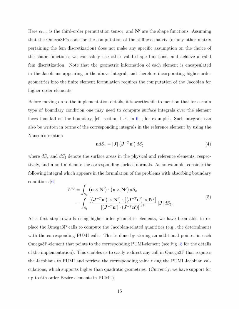
Here εkmn is the third-order permutation tensor, and Ni are the shape functions. Assuming

that the Omega3P’s code for the computation of the stiffness matrix (or any other matrix

pertaining the fem discretization) does not make any specific assumption on the choice of

the shape functions, we can safely use other valid shape functions, and achieve a valid

fem discretization. Note that the geometric information of each element is encapsulated

in the Jacobians appearing in the above integral, and therefore incorporating higher order

geometries into the finite element formulation requires the computation of the Jacobian for

higher order elements.

Before moving on to the implementation details, it is worthwhile to mention that for certain

type of boundary condition one may need to compute surface integrals over the element

faces that fall on the boundary, [cf. section II.E. in 6, , for example]. Such integrals can

also be written in terms of the corresponding integrals in the reference element by using the

Nanson’s relation

ndSx = |J |(J−Tn′

)dSξ (4)

where dSx and dSξ denote the surface areas in the physical and reference elements, respec-

tively, and n and n′ denote the corresponding surface normals. As an example, consider the

following integral which appears in the formulation of the problems with absorbing boundary

conditions [6]

W ij =

∫Sx

(n×Ni

)·(n×Nj

)dSx

=

∫Sξ

[(J−Tn′

)×Ni

]·[(J−Tn′

)×Nj

][(J−Tn′) · (J−Tn′)]1/2

|J | dSξ.(5)

As a first step towards using higher-order geometric elements, we have been able to re-

place the Omega3P calls to compute the Jacobian-related quantities (e.g., the determinant)

with the corresponding PUMI calls. This is done by storing an additional pointer in each

Omega3P-element that points to the corresponding PUMI-element (see Fig. 8 for the details

of the implementation). This enables us to easily redirect any call in Omega3P that requires

the Jacobians to PUMI and retrieve the corresponding value using the PUMI Jacobian cal-

culations, which supports higher than quadratic geometries. (Currently, we have support for

up to 6th order Bezier elements in PUMI.)

15

5.1. Results

By replacing the Jacobian calls in Omega3P with the corresponding PUMI calls we were

able to pass the current tests for meshes with quadratic curved elements, and therefore

demonstrate that the above approach works.

5.2. Future Steps

Our plan for future developments in regard to the higher-order geometries is as follows:

• Move to higher order finite element with support for higher order geometries using theapproach described above

• Once we have full support for higher order geometries we plan to compare the per-formance improvements of p-version finite element with that of the h-version finiteelement.

16

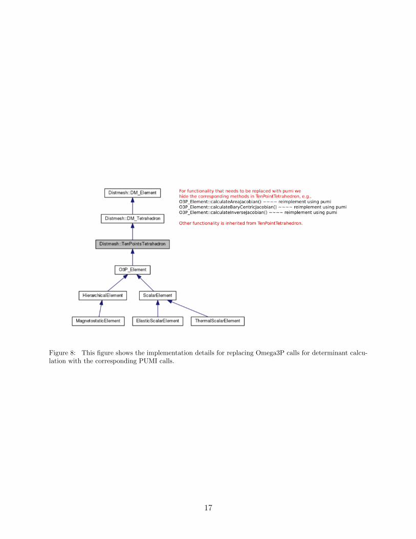
Figure 8: This figure shows the implementation details for replacing Omega3P calls for determinant calcu-lation with the corresponding PUMI calls.

17

References

[1] Albany website. http://gahansen.github.io/Albany, 2015.

[2] Saikat Dey, Mark S Shephard, and Joseph E Flaherty. Geometry representation issues

associated with p-version finite element computations. Computer methods in applied

mechanics and engineering, 150(1):39–55, 1997.

[3] Daniel A Ibanez, Ian Dunn, and Mark S Shephard. Hybrid mpi-thread parallelization

of adaptive mesh operations. Parallel Computing. Submitted, 2014.

[4] Par Ingelstrom. A new set of h (curl)-conforming hierarchical basis functions for tetrahe-

dral meshes. Microwave Theory and Techniques, IEEE Transactions on, 54(1):106–114,

2006.

[5] Kwok Ko, Arno Candel, Lixin Ge, Andreas Kabel, Rich Lee, Zenghai Li, Cho Ng, Vineet

Rawat, Greg Schussman, Liling Xiao, et al. Advances in parallel electromagnetic codes

for accelerator science and development. LINAC2010, Tsukuba, Japan, pages 1028–

1032, 2010.

[6] Lie-Quan Lee, Cho Ng, Zenghai Li, and Kwok Ko. Omega3p: A parallel finite-element

eigenmode analysis code for accelerator cavities. Technical report, 2009.

[7] Xiangrong Li, Mark S Shephard, and Mark W Beall. Accounting for curved domains

in mesh adaptation. International Journal for Numerical Methods in Engineering,

58(2):247–276, 2003.

[8] Xiao-Juan Luo, Mark S Shephard, Lie-Quan Lee, Lixin Ge, and Cho Ng. Moving

curved mesh adaptation for higher-order finite element simulations. Engineering with

Computers, 27(1):41–50, 2011.

[9] Xiao-Juan Luo, Mark S Shephard, Robert M Obara, Rocco Nastasia, and Mark W Beall.

Automatic p-version mesh generation for curved domains. Engineering with Computers,

20(3):273–285, 2004.

18

[10] Xiaojuan Luo, Mark S Shephard, Jean-Francois Remacle, Robert M O’Bara, Mark W

Beall, Barna Szabo, and Ricardo Actis. p-version mesh generation issues. In IMR, pages

343–354, 2002.

[11] Andrew G Salinger, Roscoe A Bartett, Quishi Chen, Xujiao Gao, Glen Hansen, Irina

Kalashnikova, Alejandro Mota, Richard P Muller, Erik Nielsen, Jakob Ostien, et al.

Albany: A component-based partial differential equation code built on trilinos. Techni-

cal report, Sandia National Laboratories Livermore, CA; Sandia National Laboratories

(SNL-NM), Albuquerque, NM (United States), 2013.

[12] Min Zhou, Onkar Sahni, Ting Xie, Mark S Shephard, and Kenneth E Jansen. Un-

structured mesh partition improvement for implicit finite element at extreme scale. The

Journal of Supercomputing, 59(3):1218–1228, 2012.

19