Embed Size (px)
Citation preview
IMPROVEMENTS TO THE RADIANT TIME SERIES
METHOD COOLING LOAD CALCULATION
PROCEDURE
By
BEREKET ASGEDOM NIGUSSE
Bachelor of Science in Chemical Engineering Addis Ababa University Addis Ababa, Ethiopia
1989
Master of Engineering Science in Mechanical Engineering University of New South Wales
Sydney, Australia 1998
Submitted to the Faculty of the Graduate College of the
Oklahoma State University in partial fulfillment of
the requirements for the Degree of
DOCTOR OF PHILOSOPHY December, 2007
ii
IMPROVEMENTS TO THE RADIANT TIME SERIES
METHOD COOLING LOAD CALCULATION
PROCEDURE
Dissertation Approved:
Dr. Jeffrey D. Spitler
Dissertation Adviser
Dr. Daniel E. Fisher
Dr. Lorenzo Cremaschi
Dr. Alan Noell
Dr. A. Gordon Emslie
Dean of the Graduate College

iii
ACKNOWLEDGEMENTS First I would like to express my deepest gratitude to my advisor Dr Jeffrey D.
Spitler, for his continuous guidance and support over the course of my Ph.D. degree
study. I am very grateful for his constructive advice and criticism, without which my
success would have been impossible. I would like to this opportunity to thank Dr Daniel
Fisher, Dr Alan Noell, and Dr Lorenzo Cramaschi for their time in serving as my
advisory committee members.
Next I would like to thank the US State Department for the two-year financial
support as Fulbright Scholar. Much of the work was funded by ASHRAE 1326-RP. I am
also grateful to ASHRAE for the further financial support provided to me as student
Grant-in-Aid.
Finally I would like to express my deepest appreciation for my mother, sisters,
brothers, and family members for their encouragement and unconditional love. And my
special appreciation goes to my wife Aida Mebrahtu for her support and encouragement.
iv
TABLE OF CONTENTS
Chapter Page I. INTRODUCTION......................................................................................................1 1.1 Background........................................................................................................1 1.2 Objectives ........................................................................................................13 II. REVIEW OF LITERATURE..................................................................................17 2.1 The Radiant Time Series Method ....................................................................18
2.1.1 The RTSM Procedure .............................................................................20 2.1.2 Heat Transfer Phenomena.......................................................................22 2.1.3 RTF Generation ......................................................................................27 2.1.4 Limitations of the Radiant Time Series Method.....................................28
2.2 Dynamic Modeling of Thermal Bridges ..........................................................30 2.2.1 One-Dimensional Conduction Transfer Function...................................32 2.2.2 Steady State Conduction Models ............................................................36 2.2.3 Multi-dimensional Conduction Dynamic Models ..................................39
III. RTS METHOD IMPROVEMENTS......................................................................51 3.1 New RTF Calculation Engine..........................................................................53
3.1.1 The Mathematical Model –Reduced Heat Balance Method ...................55 3.1.2 Validation of the New RTF Engine ........................................................70 3.1.3 1D Finite Volume Method PRF Generation ...........................................74 3.1.4 1D RTF Generation in Different Programming Environment................76
3.2 Improved Fenestration Model..........................................................................78 3.2.1 Development of Improved Fenestration Model......................................79 3.2.2 Radiative - Convective Split in the RTSM .............................................84 3.2.3 Application of Fenestration Model without Internal Shade....................98 3.2.4 Application of Fenestration Model with Internal Shade.........................99 3.3 Heat Losses in the RTSM Procedure .............................................................100 3.3.1 Derivation of the Mathematical Algorithm...........................................101 3.3.2 Dimensionless Loss Conductance.........................................................115 3.3.3 Performance of Improved RTSM Procedure ........................................118 3.3.4 Heat Losses in the RTSM and TFM Procedures ..................................122 3.3.5 Conclusion and Recommendation ........................................................125 3.4 Summary and Conclusions ............................................................................127
v
Chapter Page IV. PARAMETRIC STUDY OF THE RTSM PROCEDURE..................................131 4.1 Parametric Run Generation............................................................................132 4.2 Test Zone Parameters.....................................................................................134
4.2.1 Zone Geometry and Construction Fabric..............................................135 4.2.2 Thermal Mass Types.............................................................................138 4.2.3 Internal Heat Gains and Schedules .......................................................139
4.2.4 Glazing Types .......................................................................................140 4.2.5 Interior Shade Model ............................................................................142 4.2.6 Radiative-Convective Split ...................................................................143 4.2.7 Solar and Radiant Heat Gain Distribution ............................................144 4.2.8 Design Weather Days ...........................................................................145 4.3 Methodology: HBM and RTSM Implementation..........................................147
4.3.1 The HB Method Code...........................................................................148 4.3.2 The RTS Method Code .........................................................................150 4.3.3 The RTSM and HBM Models Comparison ..........................................151
4.4 Results and Discussion- Original RTSM.......................................................153 4.4.1 RTSM Peak Design Cooling Load Prediction ......................................154 4.4.2 Conclusion and Recommendation ........................................................163
4.5 Results and Discussion – Current and Improved RTSM...............................166 V. DYNAMIC MODELING OF THERMAL BRIDGES-METHODOLOGY ........175 5.1 Introduction....................................................................................................175 5.2 The Equivalent Homogeneous Layer Wall Model ........................................175
5.2.1 Steady State R-value .............................................................................178 5.2.2 Step-By-Step Procedure........................................................................178
VI. DYNAMIC MODELING OF THERMAL BRIDGES - VALIDATION ...........183 6.1 Experimental Validation ................................................................................184
6.1.1 Guarded Hot Box Dynamic Response Test Facility .............................184 6.1.2 The Test Procedure and Specimens ......................................................186 6.1.3 Experimental Determination of the CTFs.............................................190 6.1.4 The Experimental Validation Procedure...............................................194 6.1.5 The Equivalent Walls............................................................................197 6.1.6 Comparison of Conduction Heat Gains ................................................217
6.2 Inter-Model Validation ..................................................................................223 6.2.1 Numerical Validation............................................................................224 6.2.2 The R-values and the Equivalent Walls ................................................227 6.2.3 Performance of the Equivalent Walls ...................................................228
vi
Chapter Page
6.2.4 Summary and Conclusion.....................................................................231 6.3 Conclusions and Recommendations ..............................................................233 6.4 Recommendations for Future Work...............................................................236
VII. CONCLUSIONS AND RECOMMENDATIONS.............................................237 7.1 Conclusions – RTSM Improvements............................................................ 237 7.1.1 Accounting Space Heat Losses.............................................................238 7.1.2 Improvements to the RTSM Fenestration Model .................................238 7.1.3 Improvements to the RTF Generation ..................................................239 7.1.4 Developments to RTSM Implementation .............................................239 7.1.5 Parametric Study of the Performance of RTSM...................................240 7.2 Conclusion: Dynamic Modeling of Thermal Bridges....................................243 7.3 Recommendations for Future Work...............................................................245 REFERENCES ..........................................................................................................249 APPENDIX................................................................................................................259 APPENDIX A: THE NEW RTF ENGINE VALIDATION......................................259 APPENDIX B: 1D FINITE VOLUME METHHOD PRF GENERATION .............264 B.1 Derivation of 1D Finite Volume Numerical Model ......................................264 B.2 Finite Volume Method PRF Generation Validation .....................................277 APPENDIX C: RTSM IMPLEMENTATION IN OTHER COMPUTING
ENVIRONEMNTS..............................................................................................279 APPENDIX D: FENESTRATION MODELS FOR HEAT BALANCE AND RTS METHODS ................................................................................................285
vii
LIST OF TABLES
Table Page
Table 3.1 Description of zone constructions for RTF generation engine validation.................................................................................................70
Table 3.2 RMSE of the RTF of the New RTF Engine............................................71
Table 3.3 Recommended radiative / convective spits for the RTSM
procedures ...............................................................................................98
Table 4.1 Test Parameter range and levels ...........................................................134
Table 4.2 Construction Type Materials.................................................................137
Table 4.3 Thermal Mass Type materials...............................................................138
Table 4.4 Thermal and Optical Properties of glass window.................................141
Table 4.5 Optical properties of shade layers.........................................................143
Table 4.6 Mean Lighting Heat Gain Parameters from ASHRAE 1282-RP..........144
Table 4.7 Design weather conditions for the fourteen USA locations..................146
Table 4.8 RTSM and HBM component models ...................................................152
Table 4.9 Month of Annual Peak Cooling Load for zones with single pane clear glass..............................................................................................159
Table 4.10 RTSM peak cooling load extreme over predictions for glazing
without interior shades..........................................................................168
Table 4.11 RTSM peak cooling load extreme over predictions for glazing without interior shades..........................................................................171
Table 6.1 Layer-by-layer descriptions of the ASHRAE RP-515 test walls..........189
viii
Table Page
Table 6.2 Surface-to-Surface R-values of ASHRAE RP-515 Test Walls.............204
Table 6.3a Equivalent walls computed with experimentally determined R-values ....................................................................................................209
Table 6.3b Equivalent walls computed with handbook R-values ...........................210
Table 6.4a Air-to-Air CTSF of the test walls generated from experimentally
determined conduction transfer functions.............................................212
Table 6.4b Air-to-Air CTSF of the EHL walls determined with experimentally determined R-values.....................................................213
Table 6.4c Air-to-Air CTSF of the EHL walls determined with handbook R-
values ....................................................................................................214
Table 6.5 Results summary of peak heat gains and time shift ..............................221
Table 6.6 Test walls construction description inter-model validation ..................225
Table 6.7 Surface-to-surface R-value of inter-model validation test walls...........227
Table 6.8 Equivalent walls of inter-model validation test walls...........................228
Table 6.9 Peak heat gains and time shift for inter-model validation ....................229
ix
LIST OF FIGURES
Figure Page
Figure 2.1 Radiant Time Series Method represented as a nodal network. A single wall is shown with the outside surface on the left (Rees at al. 2000) ...............................................................................................19
Figure 2.2 The original RTSM cooling load calculation method represented
as flow diagram (Rees at al. 2000).......................................................21
Figure 2.3 Linear-triangular ramp temperature pulse representation....................41
Figure 3.1 Adiabatic boundary condition for RTF generation: Tso=Tsi .................58
Figure 3.2 Flow chart of solution scheme I...........................................................69
Figure 3.3 Solar RTF for lightweight construction zone with no carpet for 50% glazing fraction of the exterior facade.........................................72
Figure 3.4 Non-solar RTF for lightweight construction zone with no carpet
for 50% glazing fraction of the exterior facade ...................................72
Figure 3.5 Solar RTF for lightweight construction zone with no carpet for 50% glazing fraction of the exterior facade.........................................73
Figure 3.6 Non-solar RTF for lightweight construction zone with carpet for
50% glazing fraction of the exterior facade.........................................73
Figure 3.7 Peak heat gains calculated using finite volume method versus the State Space method PRFs ....................................................................76
Figure 3.8 Absorbed component as a fraction of total solar heat gain for
different fenestration classes................................................................83
Figure 3.9 TsIn and the corresponding MRT of heavyweight construction opaque exterior surfaces and 24°C room air temperature....................86
x
Figure Page
Figure 3.10 TsIn and the corresponding MRT for an opaque surface at peak load for three aspect ratios and 24°C room air temperature ................87
Figure 3.11 TsIn and the corresponding MRT for single pane clear glass
fenestration and 24°C room air temperature........................................89
Figure 3.12 TsIn and the corresponding MRT for south facing fenestration at peak load for three aspect ratios and 24°C room air temperature........90
Figure 3.13 Radiative fractions for fenestration in a heavyweight construction
zone and single pane clear glass with 90% glazing fraction................91
Figure 3.14 Radiative fractions for fenestration in a heavyweight construction zone and single pane clear glass with 50% glazing fraction................92
Figure 3.15 Radiative Fraction against glazing fraction of exterior facade for
heavyweight zone for five glazing types .............................................93
Figure 3.16 Radiative fractions against percent glazing of exterior facade for lightweight zone for five different glazing types at peak cooling load condition.......................................................................................96
Figure 3.17 Radiative fractions against percent glazing of exterior facade for
heavyweight zone for five different glazing types at peak cooling load condition.......................................................................................96
Figure 3.18 RTSM versus the HBM peak cooling loads for single pane clear
glass without interior shaded fenestration............................................99
Figure 3.19 Current RTSM versus the HBM peak cooling loads for single pane clear glass with interior shaded fenestration .............................100
Figure 3.20 Representation of fenestration inside surface heat balance ...............103
Figure 3.21 The improved RTSM cooling load calculation method
represented as flow diagram ..............................................................115
Figure 3.22 Dimensionless loss conductance against glazing fraction for zones with unshaded fenestration ......................................................117
Figure 3.23 Dimensionless loss conductance against glazing fraction for zone
with two exterior facades and interior shaded fenestration ...............117
xi
Figure Page
Figure 3.24 RTSM peak cooling load vs. HBM for light and heavyweight zone for single pane clear glass without internal shade.....................119
Figure 3.25 Hourly cooling load profile for lightweight zone at 50% glazing
fraction for single pane clear glass in Chicago, Illinois.....................120
Figure 3.26 Hourly cooling load profile for lightweight zone at 90% glazing fraction for single pane clear glass in Chicago, Illinois.....................120
Figure 3.27 RTSM peak cooling load vs. HBM for light and heavyweight
zone for single pane clear glass with internal shade ..........................121
Figure 4.1 Schematic of Parametric Run Generator............................................133
Figure 4.2 Zone orientation and number designations ........................................136
Figure 4.3 Structure of Heat Balance Method for a Zone ...................................149
Figure 4.4 The current RTSM cooling load calculation method represented as flow diagram..................................................................................150
Figure 4.5 RTSM annual peak cooling load versus the HBM for the USA
weather locations for single pane clear glass.....................................160
Figure 4.6 RTSM annual peak cooling load versus the HBM for the USA weather locations for double pane clear glass....................................161
Figure 4.7 RTSM annual peak cooling load versus the HBM for the USA
weather locations for double pane low-e glass ..................................161
Figure 4.8 Maximum RTSM peak cooling load over prediction against glazing fraction for the three glazing types........................................162
Figure 4.9 Current RTSM annual peak-cooling load maximum and average
over prediction for zone without interior shade.................................169
Figure 4.10 Improved RTSM annual peak-cooling load maximum and average over prediction for zone without interior shade ...................169
Figure 4.11 Current and Improved RTSM annual peak-cooling load versus
HBM for lightweight zones single pane clear glass without interior shade......................................................................................170
xii
Figure Page
Figure 4.12 Current and Improved RTSM annual peak-cooling load versus HBM for heavyweight zones with single pane clear glass without interior shade......................................................................................170
Figure 4.13 Current RTSM annual peak-cooling load maximum and average
over prediction for zones with dark roller interior shade...................172
Figure 4.14 Improved RTSM annual peak-cooling load maximum and average over prediction for zones with dark roller interior shade .....173
Figure 4.15 Current and Improved RTSM annual peak-cooling load versus
HBM for lightweight zones with single pane clear glass and dark roller interior shade ............................................................................173
Figure 4.16 Current and Improved RTSM annual peak-cooling load versus
HBM for lightweight zones with single pane clear glass and dark roller interior shade ............................................................................174
Figure 6.1 Sectional view of guarded hotbox facility (Brown and Stephenson
1993b) ................................................................................................186
Figure 6.2 Flow chart of the experimental validation procedure ........................196
Figure 6.3 Thermal bridge types: (a) sandwiched type; (b) exposed type ..........198
Figure 6.4 ASHRAE RP-515 Test Walls ............................................................203
Figure 6.5 CTSF plot for the steel stud wall (Wall#1)........................................215
Figure 6.6 CTSF plot for the steel stud wall (Wall#4)........................................216
Figure 6.7 CTSF plot for hollow block with insulation and brick exterior finish (wall#5)....................................................................................216
Figure 6.8 Heat gain for insulated steel stud wall with stucco exterior finish
(Wall#1) .............................................................................................217
Figure 6.9 Heat gain for pre-cast reinforced concrete slab with steel furring and insulation covered with gypsum board on the exterior (Wall#2) .............................................................................................218
Figure 6.10 Heat gain for pre-cast reinforced concrete slab with steel furring
and insulation with gypsum board (Wall#3)......................................218

xiii
Figure Page
Figure 6.11 Heat gain for insulated steel stud wall mounted on reinforced
concrete slab (Wall#4) .......................................................................219
Figure 6.12 Heat gain for hollow concrete block with insulation and brick on the exterior and gypsum board (Wall#5) ...........................................219
Figure 6.13 Heat gain for insulated steel stud wall with brick exterior finish
(Wall#6) .............................................................................................220
Figure 6.14 Heat gain for solid concrete block wall with insulation and granite veneer exterior finish (Wall#7)..............................................220
Figure 6.15 Summary of peak heat gains for the seven ASHRAE test walls .......222
Figure 6.16 Handbook R-value errors of the seven ASHRAE test walls..............222
Figure 6.17 Wood and steel stud walls construction details .................................226
Figure 6.18 Heat gain of a wood stud wall for periodic sol-air temperature
boundary condition ............................................................................229
Figure 6.19 Heat gain of a warm steel stud wall for steady periodic sol-air temperature boundary condition ........................................................230
Figure 6.20 Heat gain of a cold steel stud wall for steady periodic sol-air
temperature boundary condition ........................................................230
Figure 6.21 Heat gain of a hybrid steel stud wall for steady periodic sol-air temperature boundary condition ........................................................231
Figure 6.22 Handbook R-value errors compared to that of the 2D finite
volume method...................................................................................232
Figure 6.23 Peak cooling load prediction error of the equivalent walls compared to the 2D finite volume method ........................................232

xiv
1
CHAPTER I
1 INTRODUCTION 1.1 Background Design cooling load calculation methods have evolved since their inception during the
1930’s. The historical development of cooling load calculation procedures has been
strongly influenced by the development and availability of digital computing facilities,
and by the desire to provide methods that are of utility to average practicing engineers
that can be used with tabulated data (Rees et al. 2000a; Romine 1992).
It is useful to define the terms “heat gains” and “cooling load” and the relationship
between them in the context of load calculations. Heat gain is defined as the
instantaneous heat flow into a space by conduction, convection and radiation. Cooling
load is defined as the amount of heat removed from a space to keep the space air at a
fixed desired temperature. Therefore, all heat gains do not necessarily become cooling
loads: convective heat gains become cooling load instantaneously, while radiant heat
gains are first absorbed by the structure and then released by convection to become a
cooling load at a later time. Absorption and re-radiation of radiant heat gains among the
surfaces in the zone continues as long as temperature difference exits. Under some
circumstances, some of the heat gains may be conducted back out of the space.
2
The challenge in the early days of the cooling load calculation was primarily to develop
procedures to quantify the heat gains. In the 1930s peak-cooling loads were over
predicted due to failure to account for thermal mass effects of construction in the load
calculation (Houghten et al. 1932; James 1937; Kratz and Konzo 1933). Analytical
equations for computing transient conduction heat gains through homogeneous layer
constructions exposed to solar radiation were developed. Houghten, et al., (1932) used
Fourier analysis and assumed sinusoidally varying outside surface temperatures. Alford,
et al., (1939) improved this by assuming sinusoidally varying outdoor air temperature and
accounting for solar radiation separately. Despite an effort to develop a rigorous
analytical procedure for computing transient heat conduction, there was little success in
establishing a general quantitative relation suitable for practicing engineers.
The electric analogy method of predicting heat flow through walls based on the identity
of the transient heat flow and flow of electricity can be implemented experimentally and
can closely match direct thermal measurements (Paschkis 1942). An electric analog
thermal circuit of an embedded tube cooling slab model was developed using electrically
equivalent resistance, capacitance, and source terms (Kayan 1950). This allowed
determination of the slab surface temperatures, temperature isotherms in the slab and heat
transfer rates.
By the mid 1940s, the American Society of Heating and Ventilation Engineers (ASHVE),
a predecessor of the American Society of Heating, Refrigeration and Air Conditioning
Engineers (ASHRAE), developed a manual method for calculating the heat gain through
3
various external surfaces with equivalent temperature differentials (ETD) values. The
ETD values were often 20 to 40 degrees Fahrenheit above the difference between outside
and inside air temperatures (Rees et al. 2000a; Romine 1992). In the ETD method two
procedures were involved: the ETD were generated from experimentally measured
surface temperatures and conductance (Rees et al. 2000a) for transient conduction heat
gain, and the instantaneous solar heat gains through glazing were calculated using heat
fluxes and shading coefficients. The ETD method excessively overestimated cooling
load due to the assumption that the heat gains instantaneously caused cooling loads on the
system. The delays of solar heat gains before becoming cooling load were well
understood but simple quantitative relations for these effects were not available until the
1940s and 1950s. Designers made various approximations to compensate for the over
prediction of cooling loads (Romine 1992).
Transient conduction heat gain calculation procedures through external surfaces
developed using Fourier analysis assumed periodic variation of sol-air temperature as the
external driving temperature, constant indoor air temperature, and fixed outside and
inside conductance1 (Mackey and Wright 1944; Mackey and Wright 1946). The sol-air
temperature is a concept derived from the equivalent temperature (Billington 1987) used
then in UK. It is defined as the temperature that would give the same amount of heat
transfer as that of the actual outdoor air temperature and solar radiation incident on the
surface. Mackey and Wright (1946) formulated semi-empirical relations to estimate
inside surface temperatures for multi-layered walls based on an analytic solution for
1 A fixed value of combined outside conductance of 4.0 (Btu/hr⋅ft2⋅°F) is still commonly used after 60 years.
4
multi-layered walls. The damping and delay effects of the surface thermal mass on the
inside surface temperature were accounted using a decrement factor and time lag.
Developing an equation for the inside surface temperatures using the sol-air temperature
to account for the incident solar flux provided the first convenient manual procedure for
computing instantaneous heat gains. The heat gains were computed from the inside
surface temperature and room air temperature, assuming a fixed combined inside
conductance.
Later, Stewart (1948) used this procedure to tabulate the ETD for various construction
assemblies, surface exterior colors, surface orientations, latitude angles and hours of the
day. The tabulated ETD values were adjusted for use with walls and roofs overall heat
transfer coefficient, instead of combined inside conductance.
This concept was then adopted by ASHRAE as the total equivalent temperature
difference and time averaging (TETD/TA) method in the 1960s. The TETD/TA load
calculation method first introduced in the 1967 Handbook of Fundamentals (ASHRAE
1967; Rees et al. 2000a; Romine 1992). The TETD/TA method mainly involves two
steps: calculation of heat gains components from all sources and conversion of these heat
gains into cooling loads. The TETD replaced the ETD with improved tables and
equations for the equivalent temperature differences. Walls and roofs were characterized
by two parameters -decrement factor (ratio of peak heat gain to the peak heat gain that
would occur with no thermal mass in the wall) and time lag (delay in peak heat gain
compared to peak sol-air temperature). The TETD could then be calculated knowing sol-
5
air temperature, room air temperature, and decrement factors and time lags. Conversion
of the instantaneous heat gains into cooling loads using the time averaging technique is a
two step procedure: first, split the instantaneous heat gain into convective and radiant
components using recommended radiative /convective splits; second, the radiative
component of the heat gain is time averaged depending on the thermal mass of the
construction to get the cooling loads. For lightweight construction, the hourly radiant
cooling load is the radiant component of heat gain time averaged over a 2 to 3 hour
period prior to and including the time of maximum load conditions. For heavyweight
construction, the hourly radiant cooling load is the radiant component of heat gain time
averaged over a 5 to 8 hour period prior to and including the time of maximum load
conditions (ASHRAE 1967). The total hourly cooling load is the sum of the convective
component and the hourly radiant cooling load.
The work described above did not explicitly consider interactions between heat gain
components. The earliest attempt to model zone dynamics involving conduction through
the envelope, solar heat gains and the radiant exchange among surfaces and convection
between surfaces and room air utilized physical (electric and hydraulic) analogies in the
1940s and 1950s. However, the analogies remained research tools as it was not feasible
for practicing engineers to build electric circuits, nor were the insights gained reduced to
manual calculation procedures.
Leopold (1948) used a hydraulic analogy to investigate zone dynamics. The model
included thermal storage, radiation, convection, and conductions. Thermal capacitance
6
was represented by vertical tubes in series connection attached to a distribution header
connected to a storage tank, and resistances were represented by restricted tube.
Radiation absorbed by surfaces was represented by liquid flow from a pump through a
calibrated restriction, and temperatures were represented by fluid pressure. The hydraulic
model demonstrated dynamics of zones and gave some insights to the limitations the load
calculation procedures.
Despite all efforts to improve the accuracy of load calculation procedures, peak cooling
load computed using the ASHVE Guide 1952 over predicted by 16 to 32 % compared to
values measured in a small single story residential house with large glass exposure due to
failure to account for the storage effect (Gilkey et al. 1953). Similarly, a field survey
made on single family houses over a wide range of climates and construction fabrics
revealed over sizing of cooling equipment capacity due to failure to account for the
thermal mass effects of building structures (Willcox et al. 1954).
Dynamic modeling of thermal mass effects of structures and furnishing in a building was
attempted using analog computers by solving the electrical equivalent thermal circuit of
actual buildings (Willcox et al. 1954). The model used pure resistances to represent
doors, windows, blinds and infiltration. Distributed resistances and capacitances were
used to represent walls, roofs and partitions. The outdoor and indoor temperatures were
represented by potential differences. With this approach, the authors found it difficult to
construct a circuit that both had a one-to-one physical correspondence with the building,
and which gave a good match to transient thermal measurements. They did find that they
7
could “tune” a simpler circuit to give the correct dynamic response, but this has limited
usefulness for design load calculations. However, they had better success with an analog
computer, which utilizes amplifiers and allows better measurement of intermediate
values. The analog computer’s calculated response was only 7% higher than the actual
thermal measurements.
The work of Brisken and Reque (1956), in developing what they called the ‘Thermal
Response Method’, was the first attempt to use digital computers by representing a wall
using two-lump (one-resistance and two-capacitance) thermal circuit that was connected
to outdoor sol-air temperature and indoor air temperature nodes using outside and inside
combined conductance. The two differential equations for the two-lump thermal circuit
were solved using the Laplace transform method to determine the room response to a unit
square pulse applied at the sol-air temperature while the room air temperature was
constant. The method was not adopted in the ASHVE Guide, but the approach later
became the basis for development of the conduction transfer function method with a unit
triangular pulse adopted by ASHRAE for transient conduction heat gain calculations.
A procedure for computing room response factors using a detailed thermal circuit model
involving radiation exchange among inside surfaces and room furnishings, convection
between surfaces and room air, and various room heat sources was developed by Mitalas
and Stephenson (1967). An effort to provide a more rigorous load calculation procedure
led to the development of conduction transfer functions for transient conduction through
homogeneous multi-layered constructions (Stephenson and Mitalas 1971). The transfer
8
function method (TFM) for computing zone thermal response and cooling load was first
published in the 1972-Handbooks of Fundamentals (ASHRAE 1972). The method relied
on a set of tabulated room transfer function coefficients.
Given the enormous (in the 1970s) computational efforts required by the TFM and the
lack of computer resources and skills of practicing engineers there was a need for a
method that could be used manually. As a result, a simplified procedure called the
Cooling Load Temperature Difference / Cooling Load Factor (CLTD/CLF) method was
developed under ASHRAE RP-138 by Rudoy and Duran (1975). The CLTD/CLF
method is a single step load calculation procedure. CLTD values were calculated by
dividing the cooling load due to a particular wall or roof using the TFM by the U-value of
the constructions. Due to its simplicity, the CLTD/CLF method replaced the TETD/TA
methods as the ASHRAE-recommended manual load calculation procedure. However,
the CLTD/CLF method had limitations due to a lack of tabulated CLTD/CLF design data
that matched the wide range of design conditions faced by practitioners. Thus, designers
showed continued interest into TETD/TA method due to its flexibility for manual load
calculations and adaptations for various building envelope assemblies and design
locations (Romine, 1992).
ASHRAE’s continued commitment to refine load calculation procedures, to investigate
effects of different building design parameters, and to provide accurate design data led to
new research directions in the 1980s. ASHRAE-funded research project 472-RP
characterized room response based on fourteen building design parameters. Generating,
9
tabulating, and printing the whole range of the CLTD/CLF data on the basis of the
fourteen design parameters became an impractical task (Sowell 1988c). However,
ASHRAE maintained the CLTD/CLF method, which later became the Cooling Load
Temperature Difference /Solar Cooling Load / Cooling Load Factor (CLTD/SCL/CLF)
method, as a manual load calculation procedure by tabulating CLTDs for representative
families of walls and roof assemblies and developing a mapping procedure for the actual
constructions. Software for generating CLTD and CLF data based on the weighting
factors and conduction transfer function coefficients developed in ASHRAE RP−472 was
developed as part of ASHRAE RP-626 (Spitler et al. 1993b). Spitler, et al. (1993a)
introduced a new factor, the solar cooling load (SCL), for converting solar heat gain into
cooling load. Though the TFM required high computational resources, it remained the
only computational design cooling load calculation procedure recommended by
ASHRAE until the late 1990s.
The Transfer Function Method was not well received (Romine 1992) by practicing
engineers for the following reasons:
• Intimidating look of the equations
• Required iterations and convergence may take three to five successive design day
calculations
• Computer resources and a lack of computing skills also limited its implementation
for load calculations
A simple and yet reasonably accurate load calculation procedure that did not involve
iterative processes was highly desired by ASHRAE to replace the manual procedures. An
10
ASHRAE funded project (RP-875) for continued improvements of load calculation
procedures led to the development of the Heat Balance Method (HBM) (Pedersen et al.
1997) and the Radiant Time Series Method (RTSM) (Spitler et al. 1997) for calculating
peak cooling loads.
The HBM was first implemented in the 1960s by Kusuda in NBSLD, later by Walton in
1980s in Building Loads Analysis and System Thermodynamics (BLAST) and in
Thermal Analysis Research Program (TARP) as cited by Pedersen, et al. (1997).
However, a complete description of the procedure for load calculation purposes had not
been available. The first complete description of the heat balance method formulation
starting from the fundamental principles, and covering implementation and solution
techniques as applied for peak cooling load calculation was presented by Pedersen, et al.,
(1997). Since the heat balance method is based on the fundamental principles of the
physics involved, it is commonly used as a reference model for simplified load
calculation programs.
The RTSM closely followed the HBM hourly cooling load profile and in most cases
slightly overpredicted the peak cooling load; however, the over predicted peak cooling
load was significant for zones with large amount of single pane glazing and cool design
weather conditions (Rees et al. 1998). The radiant time series method (RTSM) was
developed as a spreadsheet method intended to replace the TETD/TA and the
CLTD/SCL/CLF methods. It also effectively replaced the TFM. The radiant time series
method (RTSM) as a simplified load calculation procedure was adopted as a
11
nonresidential building load calculation procedure by ASHRAE and published in
Pedersen, et al. (1998) and the 2001 −Handbook of Fundamentals (ASHRAE 2001).
Experimental validation of the heat balance and the radiant time series methods has been
done in test cells at Oklahoma State University (Chantrasrisalai et al. 2003; Iu et al.
2003).
ASHRAE research project RP-942 compared the peak cooling load predictions made
with the RTSM to those made with the heat balance method (HBM) using a parametric
run investigation tool (Rees et al. 1998; Spitler and Rees 1998). Although ASHRAE
942-RP identified building design parameters that lead to over predictions of peak
cooling load, the project did not result in design guidance for practicing engineers.
The radiant times series method (RTSM) has effectively replaced the manual load
calculation procedures and has attracted interest due to:
Its amenability to spreadsheet implementations as opposed to the Transfer
Function Method, which requires iteration.
Captures and depicts the physics involved in the Conduction Time Series Factor
(CTSF) and Radiant Time Factor (RTF) coefficients, unlike the Transfer Function
Method.
Has essentially the same accuracy as the TFM.
12
However, the RTSM also has the same approximations as the TFM that, in some cases,
lead to over prediction of peak-design cooling load:
The RTSM replaces the outside heat balance by an exterior boundary condition
known as the sol-air temperature, which allows the use of fixed combined
conductance of convection and radiation.
The RTSM computes the radiant heat gain from the interior surfaces as if they all
radiate to the room air temperature instead of performing inside surface and room
air heat balances. This allows treatment with a linearized radiation coefficient,
which is combined with the convection coefficient. This assumption can over
predict the instantaneous heat gain, which again contributes to the RTSM peak
cooling load overprediction.
The RTSM uses an adiabatic boundary condition when computing Radiant Time
Factors (RTF), causing the RTF to always sum to one. When these RTF are used,
this approach conserves the entire solar and internal heat gains during conversion
to cooling load, and there is no way that the RTSM can account for any heat gains
conducted back out. As a result, the RTSM tends to over predict the peak-cooling
load when there is a large amount of single pane glazing or other highly
conductive surfaces.
The resulting over predictions was shown in 942-RP to be as high as 37%. It would be
very helpful for designers to have guidance as to when the RTSM is likely to gives
significant overprediction.
13
1.2 Objectives The previously published research in the RTSM cooling load calculation procedure has
only identified the likely over of peak cooling load and the conditions favorable for over
prediction but non them provided a procedure for accounting the heat gain loss and did
not provide guidance on the limitation of the RTSM. Therefore, one of the objectives of
this thesis is to develop an algorithm that reduces the RTSM peak cooling load likely
over prediction significantly and establish the limitations of the RTSM in a form of
design guidance. Furthermore, ten years of experience with the RTSM has indicated
several improvements that would be helpful for design engineers. These include an
improved RTF generation procedure, developing a numerical procedure for periodic
response factor generation, updated fenestration modeling and investigated a procedure
for treating thermal bridges. These improvements are discussed briefly below.
The RTSM needs radiant time factors (RTF) for the zone to be analyzed. The ASHRAE
Handbook of Fundamentals (ASHRAE 2001; ASHRAE 2005) has given tabulated RTF
for specific cases, but the accuracy resulting from users choosing the “nearest” zones has
not been investigated. The original presentation of the procedure utilized a full blown
HBM program to generate the RTF. While this approach works, the HBM program has
many features and data that are not needed for generating RTF. Therefore, one of the
objectives of this thesis is to develop a simplified procedure and implement the algorithm
for computing RTF, as described in Section 3.1. Also investigated is a direct method of
calculating periodic response factors as an alternative to converting conduction transfer
function coefficients back to response factors for use in the RTF generation procedure. A
14
one-dimensional finite volume numerical fully-implicit formulation for generating
periodic response factor will be developed. The finite volume periodic response generator
and the simplified RTF generator algorithm will also be implemented in other computing
environments. Furthermore, the RTF generation has been investigated with constant
radiation coefficient with the intent of reducing the computational time.
The radiant time series method load calculation procedure was developed based on the
shading coefficients and optical properties of double-strength glass for computing solar
heat gains. Developments in fenestration models and availability of a new set of
fenestration data – solar heat gain coefficients - replaced the use of shading coefficients
in fenestration modeling. Moreover, the shading coefficient data are no longer available.
Therefore, one of the objectives of this thesis is investigation of a new fenestration model
using window manufacturer’s data and the new set of tabulated glazing and fenestration
data available in the ASHRAE’s Handbook of Fundamentals as presented in Section 3.2.
Improved fenestration model for the RTSM will be investigated and integrated that make
use of these new developments. Moreover, a new set of radiative / convective splits for
fenestration solar and conduction heat gains will be established.
It has been identified that the likely over prediction of the RTSM procedure is due to
failure to account for the space radiant heat gains conducted back to the outside. In this
thesis an algorithm for accounting the radiant heat gain loss by conduction will be
derived and investigated in Section 3.3.1. The procedure accounts for solar and internal
radiant heat gains conducted back out through fenestrations and highly conductive mass
15
less surfaces. Furthermore, the likely overprediction of peak cooling load by the RTSM
will be investigated parametrically over a wider range of building design parameters to
characterize its limitations and develop design guidance for practicing engineers. This is
covered in Chapter Four.
Another challenge faced by designers is the treatment of thermal bridges in wall and roof
constructions. Steady state treatment of thermal bridges is covered in the ASHRAE
Handbook of Fundamentals (ASHRAE 2005). Dynamic modeling of thermal bridges has
been a research interest in building energy and load calculation applications for about two
decades. Despite repeated efforts to develop multi-dimensional conduction models
capable of dynamic modeling of thermal bridges, these models have never been
integrated into design load calculation procedures for several reasons. Therefore, another
objective of this thesis is to investigate an approximate one-dimensional dynamic model
of thermal bridges that can be directly implemented into design cooling load calculation
procedures, and develop design recommendations usable by practicing engineers. This is
covered in Chapters Five and Six.
Before addressing these three chapters, the thesis gives an in-depth literature review of
the Radiant Time Series Method and the treatment of thermal bridges in Chapter Two.
Improvements to the Radiant Time Series Method procedure are discussed in Chapter
Three. Parametric investigation of the Radiant Time Series Method to establish the
limitations based on adapted fenestration model is covered in Chapter Four. Chapters
Five and Six deal with approximate one-dimensional dynamic modeling of thermal

16
bridges methodology and the validation, respectively. Conclusions and recommendations
for future work are given in Chapter Seven.
17
CHAPTER II
2 REVIEW OF LITERATURE
The literature review covers two separate topics related to building energy analysis and
load calculation methods. The first section deals with developments in Radiant Time
Series method, and the second section deals with dynamic and steady state modeling of
thermal bridges.
The first part of the literature survey (Section 2.1) describes the development of the
Radiant Time Series Method (RTSM) as a simplified design cooling load calculation
procedure, discusses the key assumptions introduced to derive the RTSM procedure, and
explains in detail the limitation of the RTS method in predicting the peak design cooling,
and discusses the necessary conditions for the RTSM peak cooling load overprediction.
The second part of the literature survey (Section 2.2) deals with dynamic and steady state
modeling of thermal bridges in relation to building energy analysis and load calculation
program. It discusses the importance of steady state and dynamic modeling of thermal
bridges in building energy analysis and load calculation application, reviews previously
published dynamic modeling techniques for thermal bridges and explains why these
models have not been adopted.
18
It also presents a brief summary of response factors and conduction transfer functions and
the associated one-dimensional conduction modeling procedures. In addition it
summarizes recommended approximate procedures for steady state analysis of thermal
bridges.
2.1 The Radiant Time Series Method
The Radiant Time Series Method (RTSM) was introduced as a simplified design load
calculation procedure (Spitler et al. 1997). The RTSM was intended to replace
ASHRAE’s simplified load calculation procedures: the cooling load temperature
difference/solar cooling load/cooling load factor (CLTD/SCL/CLF) method, the total
equivalent temperature difference/time averaging (TETD/TA) method, and the Transfer
Function Method (TFM). The radiant time series method can be thought as a two-stage
process (Spitler et al. 1997). The first stage of this process is to calculate all the radiant
and convective heat gains of the zone. The second stage is the conversion of these gains
into contributions to the cooling load on the zone air.
Several key approximations have been employed in simplifying the RTSM in order to
avoid the iteration steps in the procedure so as to make the method suitable for
spreadsheet implementation. The first simplifying assumption in the radiant time series
method is the treatment of exterior and interior convection and radiation coefficients
using combined constant conductance. This simplification in effect entails the assumption
that surfaces exchange long wavelength radiation with air node. This assumption allows
19
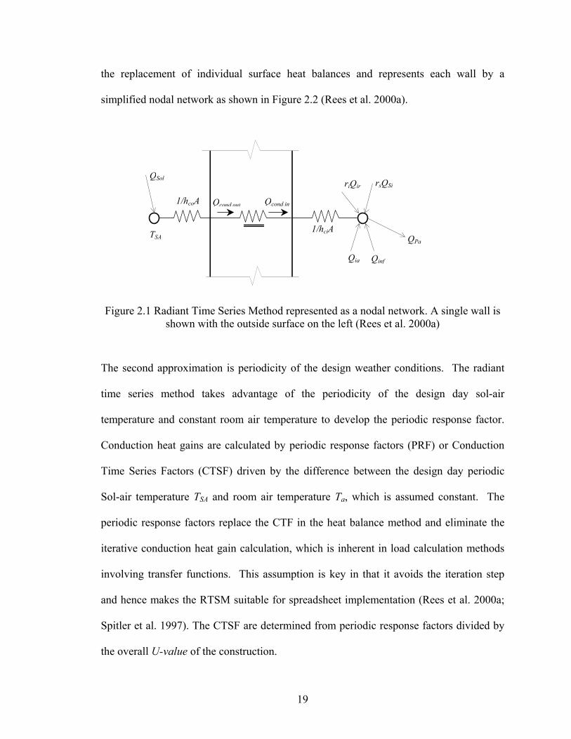
the replacement of individual surface heat balances and represents each wall by a
simplified nodal network as shown in Figure 2.2 (Rees et al. 2000a).
QinfQia
riQir rsQSi
QPa
QSol
TSA
1/hcoA
1/hciA
Qcond,out Qcond,in
Figure 2.1 Radiant Time Series Method represented as a nodal network. A single wall is
shown with the outside surface on the left (Rees et al. 2000a)
The second approximation is periodicity of the design weather conditions. The radiant
time series method takes advantage of the periodicity of the design day sol-air
temperature and constant room air temperature to develop the periodic response factor.
Conduction heat gains are calculated by periodic response factors (PRF) or Conduction
Time Series Factors (CTSF) driven by the difference between the design day periodic
Sol-air temperature TSA and room air temperature Ta, which is assumed constant. The
periodic response factors replace the CTF in the heat balance method and eliminate the
iterative conduction heat gain calculation, which is inherent in load calculation methods
involving transfer functions. This assumption is key in that it avoids the iteration step
and hence makes the RTSM suitable for spreadsheet implementation (Rees et al. 2000a;
Spitler et al. 1997). The CTSF are determined from periodic response factors divided by
the overall U-value of the construction.
20
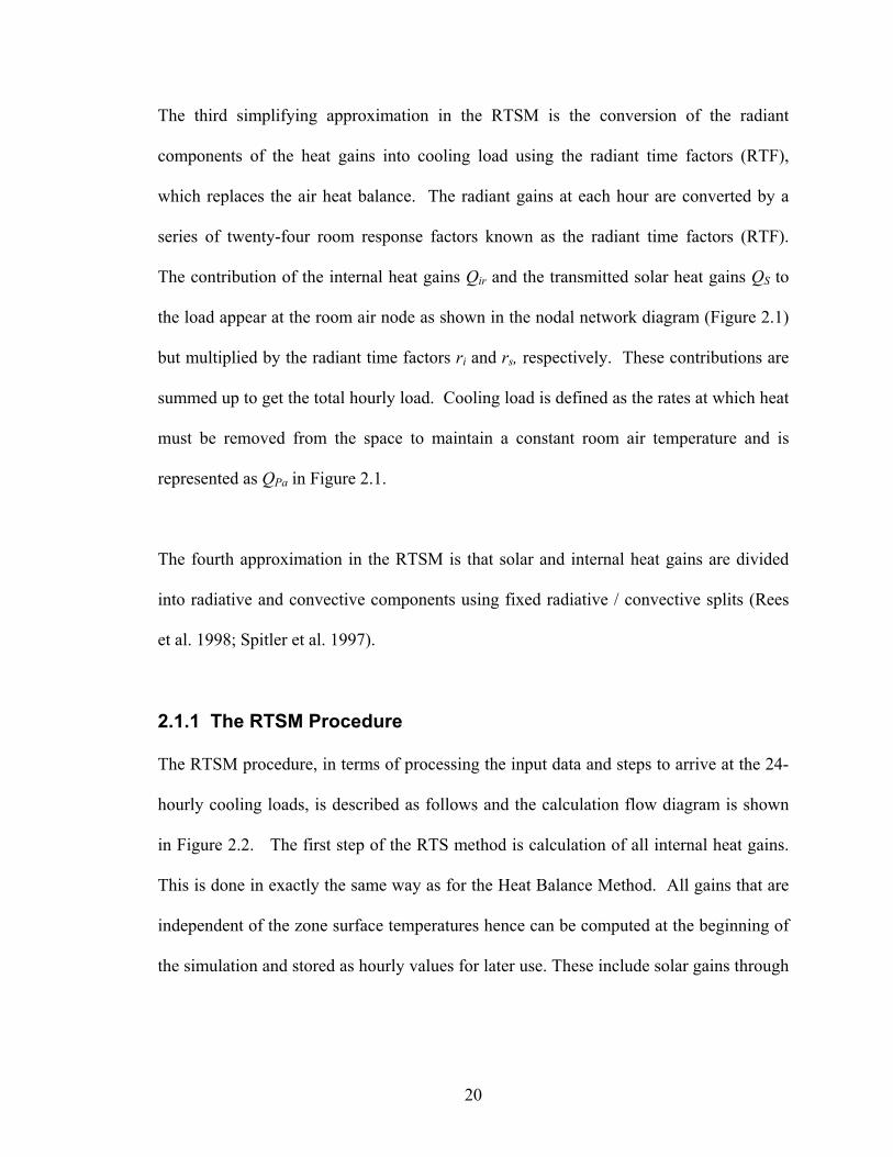
The third simplifying approximation in the RTSM is the conversion of the radiant
components of the heat gains into cooling load using the radiant time factors (RTF),
which replaces the air heat balance. The radiant gains at each hour are converted by a
series of twenty-four room response factors known as the radiant time factors (RTF).
The contribution of the internal heat gains Qir and the transmitted solar heat gains QS to
the load appear at the room air node as shown in the nodal network diagram (Figure 2.1)
but multiplied by the radiant time factors ri and rs, respectively. These contributions are
summed up to get the total hourly load. Cooling load is defined as the rates at which heat
must be removed from the space to maintain a constant room air temperature and is
represented as QPa in Figure 2.1.
The fourth approximation in the RTSM is that solar and internal heat gains are divided
into radiative and convective components using fixed radiative / convective splits (Rees
et al. 1998; Spitler et al. 1997).
2.1.1 The RTSM Procedure
The RTSM procedure, in terms of processing the input data and steps to arrive at the 24-
hourly cooling loads, is described as follows and the calculation flow diagram is shown
in Figure 2.2. The first step of the RTS method is calculation of all internal heat gains.
This is done in exactly the same way as for the Heat Balance Method. All gains that are
independent of the zone surface temperatures hence can be computed at the beginning of
the simulation and stored as hourly values for later use. These include solar gains through
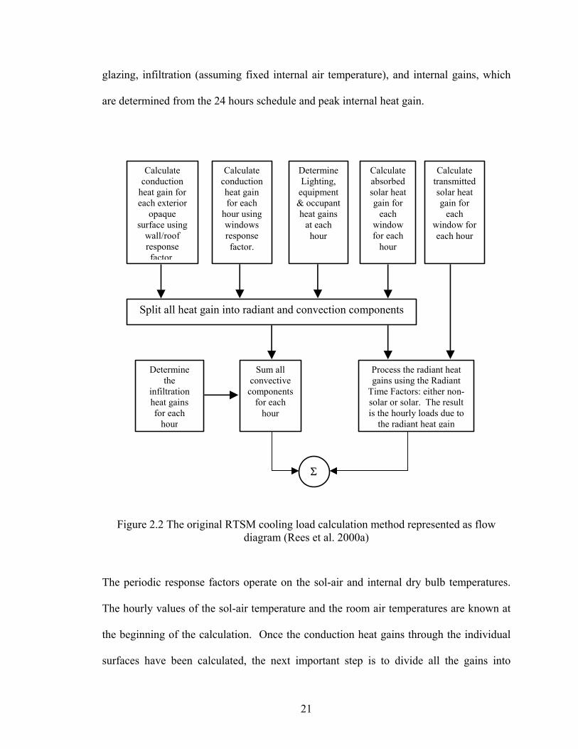
21
glazing, infiltration (assuming fixed internal air temperature), and internal gains, which
are determined from the 24 hours schedule and peak internal heat gain.
DetermineLighting,
equipment& occupant heat gains
at each hour
Calculate conduction heat gain for each
hour using windows response factor.
Calculate conduction
heat gain for each exterior
opaque surface using
wall/roof response factor,
Calculate transmitted solar heat gain for
each window for each hour
Split all heat gain into radiant and convection components
Determine the
infiltration heat gains for each
hour
Sum all convective
components for each
hour
Process the radiant heat gains using the Radiant
Time Factors: either non-solar or solar. The result is the hourly loads due to
the radiant heat gain
Σ
Calculate absorbed solar heat gain for
each window for each
hour
Figure 2.2 The original RTSM cooling load calculation method represented as flow diagram (Rees et al. 2000a)
The periodic response factors operate on the sol-air and internal dry bulb temperatures.
The hourly values of the sol-air temperature and the room air temperatures are known at
the beginning of the calculation. Once the conduction heat gains through the individual
surfaces have been calculated, the next important step is to divide all the gains into
22
radiant and convective components. This is done using fixed radiative / convective splits
for each type of heat gains.
The second stage of the RTS calculation procedure is to convert all the heat gains into
contributions to the load at the air node. Convective components of the gains make
instantaneous contributions to the cooling load while the radiant components of the heat
gains are converted to cooling loads by means of the radiant time factors (RTF). The
hourly contributions of the radiant gain to the cooling load are calculated from the 24-
hourly radiant gains and the RTF. The radiant time factors are zone dynamic response
characteristic, which are dependent on the overall dynamic thermal storage characteristics
of the zone and defines how the radiant gain at a given hour is redistributed in time to
become contributions to the cooling load at future hours. The contributions of the past
and current radiant gains are simply added to the hourly convective gains to give the
hourly cooling load.
2.1.2 Heat Transfer Phenomena
This section describes the specific practices and assumptions used by the RTSM to model
some of the principal zone heat transfer mechanisms.
Exterior Convection and Radiation
The RTS Method uses a fixed exterior surface conductance combined with a sol-air
temperature to model exterior convection and radiation. This is one of the first
simplifying assumptions of the radiant time series method.
23
Transient Conduction Heat Transfer
The RTS Method treats external and internal excitation of conduction heat flow
separately. In the RTS procedure, transient conduction heat transfer due to external
excitation is modeled using a set of 24 periodic response factors. Given the constant zone
air temperature Ta and the current and 23 past values of sol-air temperature TSAθ, the
current hour’s conduction heat gain per unit surface area is given by:
( )∑=
− −=23
0,,
'',,
jajiSAPjticond TTYq δθ& (2.1)
where,
'',, ticondq& = the current hour conduction through the ith surface, Btu/h⋅ft2 (W/m2)
PjY = the periodic response factors at j hours from the present, Btu/h(W)
δθ jiSAT −,, = the sol-air temperature of the ith surface j hour from the present, °F(°C)
aT = the constant room air temperature, °F(°C)
The periodic response factors YPj include both the interior and exterior surface
conductance. Periodic response factors can be computed from response factors (Spitler et
al. 1997), from the generalized form of the CTFs (Spitler and Fisher 1999a), and
frequency domain regression method (Chen and Wang 2005). The sol-air and inside
temperatures are known at the beginning of the calculation, therefore the heat gains due
to conduction can be calculated straightforwardly without the need for any iteration,
which makes the RTSM amenable for spreadsheet implementation. These gains
subsequently have to be divided into radiant and convective components.
24
Interior Convection and Radiation
The RTS Method uses fixed combined interior radiation and convection conductances.
The convection and radiation coefficients are added (as a resistance) into the wall. This
approach, though it simplifies the procedure, has the effect of having the wall radiating to
the zone air temperature. In most cases, this causes the RTSM to slightly over-predict the
peak cooling load (Rees et al. 2000a).
The RTS Method uses radiant time factors (RTF) to convert and redistribute the radiant
part of the conducted gain. Analogous to periodic response factors, radiant time factors
are used to convert the cooling load for the current hour based on current and past radiant
gains. The radiant time factors are defined such that r0 represents the portion of the
radiant gains convected to the zone air in the current hour. r1 represents the portion of the
previous hour’s radiant gains that are convected to the zone air in the current hour, and so
on (Spitler and Fisher 1999b). The cooling load due to radiant heat gain is given by:
∑=
−=23
0jjtjt qrQ δ (2.2)
Where
tQ = the current hour cooling load, Btu/h(W)
δjtq − = the radiant gain at j hours ago, Btu/h(W)
jr = the jth radiant time factor, Btu/h(W)
25
Transmitted and Absorbed Solar Radiation
Calculation of transmitted and absorbed solar radiation associated with fenestration is a
very important part of the design cooling load calculation procedure. The response of the
zone is dependent not only on the value of the transmitted and absorbed solar energy but
also on its distribution in the zone. Two simple procedures applicable for load
calculation purposes have evolved: (1) the use of normal solar heat gain coefficient and
transmittance and absorptance correction for angle dependence using a reference standard
DSA glass angle correction coefficients (Spitler et al. 1993a), (2) the use of angle
dependent beam solar heat gain coefficient and constant diffuse solar heat gain
coefficient tabulated values (ASHRAE 2005). The first approach allows separate
treatment of transmitted and absorbed solar radiation. Though transmitted and absorbed
components are calculated separately, the procedure is based on approximate analysis
analogous to the concept of shading coefficient. This was adopted as a standard
procedure but with demise of the shading coefficients a new procedure is needed.
The second approach is used in a combined treatment of transmitted and absorbed
components. In the second approach the solar heat gain coefficient includes both the
transmitted portion of the solar heat gain and the inward flow fraction of the absorbed
component. This therefore precludes the separate treatment of the absorbed solar heat
gain, which has both radiative and convective components. Likewise, the RTSM uses the
solar radiant time factor to convert the beam and diffuse solar heat gains into cooling
loads. The diffuse solar gains are treated in a similar way to internal short and long
wavelength radiant gains. As noted previously in the discussion on internal convection
26
and radiation heat transfer, some of the solar radiation that is re-radiated can be
conducted to the outside. The RTSM cannot account for this, and so for some zones and
design weather condition tends to over-predict the cooling loads.
Internal Heat Gains
In the radiant time series method the hourly schedules and peak gain rate for the three
type of internal heat gains (e.g. people, lights, and equipment) are specified by the user
along with the respective radiative/convective splits. Though the split between radiative
and convection actually depends on the zone airflow rates and surface temperatures,
constant values are used even in detailed building energy analysis programs. In the
RTSM the radiative component heat gain contribution on the cooling load is estimated
with the radiant time factors. The RTSM does not account for the portion of the radiant
gain that is conducted to the outside and so for some zone constructions tends to over-
predict the cooling loads. The degree of overprediction depends on the zone construction
conductance, and design weather conditions. This has been one of the limitations of the
RTSM procedure and is discussed in Section 2.1.4.
2.1.3 RTF Generation
Radiant time factors (RTF) are dynamic response characteristics of a zone when a zone is
excited by unit heat gain pulse. (Spitler et al. 1997) described two procedures for
generating RTF coefficients. The first method uses a load calculation program based on
the heat balance method (Pedersen et al. 1997).
27
The radiant time factors are generated by driving a heat balance model of the zone with a
periodic unit pulse of radiant energy under adiabatic wall conditions. The radiant time
factors are therefore different for every combination of zone construction and geometry.
In principle, they are also different for every chosen distribution of radiant pulse. Thus far
two types of distributions have been commonly used for a given zone (Spitler et al.
1997). One is found assuming an equal distribution (by area) of radiant pulse on all zone
surfaces and is used for all diffuse radiant gains. A second set is found with the unit
pulse of radiant energy added at the floor surface and in some cases to the furniture as
well to treat beam solar gains. The conversion of radiant gains by the use of radiant time
factors, where there is no requirement for knowledge of past temperatures or cooling
loads, again avoids the iteration processes.
The second method demonstrated by (Spitler and Fisher 1999b) is to generate radiant
time factors directly from a set of zone weighting factors using the existing ASHRAE
database (Sowell 1988a; Sowell 1988b; Sowell 1988c). This approach would use a
computer program to map a given zone to the fourteen zone characteristic parameters in
the database and transform the weighting factors to radiant time factors using matrix
manipulation. However, the custom weighting factors do not represent all possible zone
constructions. Use of a weighting factor database requires some approximations to fit the
fourteen selection parameters. Therefore, development of an RTF generating tool that
fits practical design condition is essential for RTSM implementations.
28
One important assumption in calculating the radiant time factors is imposing adiabatic
boundary condition for all surfaces in the zone. As the consequence of this assumption
the radiant pulse used to generate the radiant time factors is then only redistributed in
time, otherwise its energy is entirely conserved in the zone. In the RTSM, since no solar
and internal radiant heat gains are conducted out of the zone, this often leads to slight
over-prediction of the peak-cooling load. However, for zones with large amount single
pane glazing, and cooler summer design weather conditions, a significant portion of the
radiant heat gains can be conducted out, and those never become part of the cooling load.
In these cases a much larger over-prediction relative to the heat balance method is
expected (Rees et al. 2000a; Rees et al. 1998; Spitler et al. 1997).
2.1.4 Limitations of the Radiant Time Series Method
Quantitative comparison with the heat balance method shows that the RTSM tends to
over predict the peak cooling loads (Rees et al. 1998; Spitler et al. 1997). Parametric
investigations conducted for 945 zones cases showed that the peak load is slightly over
predicted (Spitler et al. 1997). The heat balance method uses a detailed fundamental and
rigorous mathematical model for the outside and inside surface heat balance. For
medium and light weight construction, in particular zones with large amount of single
pane glazing, the peak loads were over predicted significantly. In another similar study
(Rees et al. 1998) made quantitative comparison of 7,000 different combinations of zone
type, internal heat gains, and weather day. The result shows that the RTSM cooling load
profile closely follows that of the heat balance cooling load; however, it over predicted
the peak load for majority of the test cases when a radiative heat gain is large and zones

29
are made with large amount of single pane glazing. For a heavy weight construction mid-
floor, northeast corner zone, with 90% of the exterior wall area consisting of single-pane
glass (Rees et al. 1998) the RTSM over predicted the peak-cooling load by 37%. Three
main reasons have been pointed out for peak cooling load over prediction: (1) the use of
adiabatic boundary condition for the RTF generation, (2) combined treatment and
constant assumption of convection and radiation coefficients, which makes the zone
internal surfaces to radiate to the room air, and (3) simplification of the sol-air
temperature calculations.
Rees et al. (1998) concluded that the RTS method enforces conservation of radiant heat
gains by ignoring the heat gain conducted to the outside environment as the principal
reason for over prediction of peak cooling load. For internal surfaces with conditioned
adjacent zones, the adiabatic boundary condition is a reasonable approximation; however,
for external surfaces the adiabatic boundary condition in some cases very conservative
approximation. Zones for which the peak design cooling load occurs in winter or zones
located at lower design weather temperatures can be shown (with the HBM) to conduct a
large amount of heat gains through the exterior surfaces with very low conductance (e.g.
single pane glazing windows). On the other hand, the RTSM conserves the entire radiant
heat gains and has no procedure to account for the heat gain conducted to the outside.
Therefore, the RTSM over predicts the peak design cooling load slightly for hot and
warm cooling design weather locations, while it tends to over predicts more and more for
cold design weather conditions.
30
Experimental validation of radiant time series cooling load calculation method revealed
that reflection loss of solar heat gain from the zone with high glazing fraction is
significant (Iu et al. 2003). Though the re-reflection and direct transmission losses can be
computed they require detailed input data of glazing optical properties, zone geometry
and orientations. In fact this phenomenon is likely to cause significant loss only in highly
glazed buildings.
2.2 Dynamic Modeling of Thermal Bridges
Dynamic modeling of thermal bridges has been an area of interest in building energy
analysis and design load calculation programs. Building energy analysis and load
calculation programs developed in the USA use one-dimensional conduction transfer
functions to predict heat conduction through the building envelope. However, many wall
and roof constructions contain composite layers (e.g. steel studs, and batt insulation) that
lead to local multidimensional heat conduction. The element with very high thermal
conductivity is often referred to as a thermal bridge. Thermal bridges are important for
both steady state and dynamic heat conduction.
Several publications (Brown et al. 1998; Carpenter et al. 2003b; Kosny and Christian
1995b; Kosny et al. 1997b; Kosny and Kossecka 2002; Kosny et al. 1997c) indicate that
one-dimensional approaches cannot predict heat transmission through building envelopes
without errors, especially for walls with thermally massive elements and a high disparity
in the thermal conductivity of layer materials. Numerical studies indicate that thermal
bridge effects of steel stud walls can reduce the thermal resistance of the clear wall by up
31
to 50% (Kosny et al. 1997a). Similar studies on metal frame roofs showed that the
thermal bridge effect reduces the effective thermal resistance of the clear cavity values by
as high as 75% (Kosny et al. 1997c).
However, there is a limitation in the use of one-dimensional response factor or
conduction transfer functions methods when it comes to analysis of composite walls such
as stud walls. This is a common problem in modeling heat conduction in steel stud walls
and the ground where one-dimensional analysis cannot predict the heat conduction
without significant error. Multi-dimensional heat conduction effects are either ignored or
not accounted properly. The one-dimensional analysis may be valid for homogeneous
layer wall; however, at the edges and corners, heat transfer significantly deviates from
that of the one-dimensional analysis. In practice, the edge and corner effects are simply
ignored. Numerical and experimental investigations showed that ignoring the edge effects
could under predict the heat transmission by over 10% (Davies et al. 1995). However,
for portions of walls not near the edges, one-dimensional analysis can be a reasonable
approximation for lightweight walls without significant thermal conductivity disparity,
such as those made from wood studs (Davies et al. 1995). Therefore, the need for multi-
dimensional transient heat conduction models in building energy analysis and load
calculation programs is crucial for accurate prediction of building energy consumption
and peak load estimation; hence, it is also necessary for reliable HVAC equipment sizing
and thermal comfort prediction. The following section discusses the one-dimensional
dynamic conduction modeling commonly used in load calculation and energy analysis
programs in the USA.
32
2.2.1 One-Dimensional Conduction Transfer Functions
Transient conduction heat transfer through building envelopes can be calculated using
lumped parameter methods, numerical methods, frequency response methods and
conduction transfer function methods. Conduction transfer functions have been used
most commonly in lead calculation and building energy analysis programs due to their
computational efficiency and accuracy. The response factors are time series solutions of
transient heat conduction that relate the current heat flux terms to current and past
temperatures. Conduction transfer function coefficients are derived from response
factors, which are determined using Laplace transform method (Kusuda 1969; Mitalas
1968; Stephenson and Mitalas 1971), or numerically (Peavy 1978). Conduction transfer
function coefficients can be also determined directly using frequency-domain regression
(Wang and Chen 2003), stable series expansion based on the Ruth stability theory (Zhang
and Ding 2003), and State Space method (Seem 1987; Strand 1995). The next sections
presents the use of response factor and transfer function coefficients in one-dimensional
conduction.
Heat conduction through building structures is represented by one-dimensional partial
differential heat equation and the Fourier’s law of heat conduction as follows:
t
txTcx
txqp
∂∂
=∂
∂ ),(),('' ρ (2.3)
xtxTktxq
∂∂
−=),(),('' (2.4)
33
Where
q” = is the heat flux, (W/m2 K)
T = is the temperature, (oC)
k = is the thermal conductivity, (W/m K)
ρ = is the density, (kg/m3)
cp = is the specific heat of the solid, (kJ/kg K)
The solution of equations 2.3 and 2.4 can be represented as time series solutions called
response factors. The time series solution of the heat conduction equation is determined
for a unit triangular ramp excitation of the temperatures on both the internal and external
surfaces of a wall. The response factors can be determined using Laplace Transform
method (Clarke 2001; Hittle 1992; Kusuda 1969; Stephenson and Mitalas 1971),
numerical methods (Peavy 1978), and time domain methods (Davies 1996). The current
heat flux at interior surface of the wall '',tiq& in terms of current and past boundary
temperatures as inputs and the response factors is given by:
∑∑∞
=+−
∞
=+− −=
11,
11,
'',
nnnton
nntiti YTZTq& (2.5)
The heat flux at the external surfaces '',toq& is given by:
∑∑∞
=+−
∞
=+− −=
11,
11,
'',
nnnto
nnntito XTYTq& (2.6)
34
Where
'',tiq& : heat flux at the interior surfaces at time step t, W/m2
'',toq& : heat flux at the external surfaces at time step t, W/m2
Ti,t-n+1: interior boundary temperature at time step t-n+1, oC
To,t-n+1: exterior boundary temperature at time step t-n+1, oC
X: is the self-coupling response factor; the heat flux at the exterior surface for
triangular ramp input of the exterior boundary temperature and zero
interior boundary temperature (W/m2 K).
Y: is the cross coupling response factor; the heat flux at either surface for
triangular ramp input of the boundary temperature at the other surface,
(W/m2 K).
Z: is self-coupling response factor of the interior surface for triangular ramp
input of the boundary temperature at the interior surface and zero exterior
boundary temperature, (W/m2 K).
The primary advantage of the response factor method is that for a given building
structure, assuming constant thermo-physical properties, the response factors need to be
determined only once. Numerical methods such as finite difference or finite element
methods generally require high computational time; however, they allow variable time
step and variable thermo-physical property simulations.
Conduction transfer function methods are further refinements of response factor methods.
The replace many of the higher order terms of the response factors and the past
35
temperatures with the past heat fluxes; hence, use fewer coefficients (Hittle, 1992)
(McQuiston et al. 2005; McQuiston 2000). The heat fluxes at the interior and exterior
surfaces of a wall in terms of conduction transfer functions are given by:
∑ ∑∑= =
−+−=
+− +−=M
m
M
mmtimmtomk
M
mmtimkti qFTYTZq
1 1,1,,
11,,
'', (2.7)
∑ ∑∑= =
−+−=
+− +−=M
m
M
mmtommtomk
M
mmtimkto qFTXTYq
1 1,1,,
11,,
'', (2.8)
Where
Xk,m: the mth conduction transfer coefficient for the exterior self-coupling term
of order k, (W/m2 K)
Yk,m: the mth conduction transfer coefficient for the cross coupling term of order
k, (W/m2 K)
Zk,m: the mth conduction transfer coefficient for the interior self-coupling term
of order k, (W/m2 K)
Fm: is defined as the flux history term coefficients (-).
2.2.2 Steady State Conduction Models
Multi-dimensional and in particular two-dimensional steady state conduction models
have been used to study and investigate the accuracy of the approximate one-dimensional
thermal resistance calculation procedures for thermal bridges. Studies made on multi-
dimensional steady state heat conduction analysis of composite walls have indicated that
the heat fluxes deviate significantly from that of an approximate one-dimensional heat
36
conduction models that ignore the thermal bridges. This has been demonstrated using
numerical and experimental analysis of steady state heat conduction in building wall
specimens (Barbour and Goodrow 1995; Brown et al. 1998; Carpenter and Schumacher
2003; Kosny and Christian 1995a; Kosny and Christian 1995c; Kosny et al. 1997a;
Kosny et al. 1997b; Thomas and Antar 1998). Compared to dynamic analysis, steady
state models for heat transfer of thermal bridges are well developed. The next section
briefly discusses ASHRAE’s recommended approximate one-dimensional steady heat
conduction models.
Approximate Steady State Models
Steady state heat transfer through composite material walls is commonly treated with
one-dimensional models that utilize some approximations in representing the thermal
resistance of composite walls. ASHRAE recommends the following methods: isothermal
plane method, parallel path method, the zone method and modified zone method and
insulation/framing adjustment factor method to compute the overall thermal resistance
based on qualitative criteria (ASHRAE 2005).
Isothermal Plane Method
This method assumes that for layer materials with high thermal conductivity the
temperature at each plane remains isothermal. Composite layers sandwiched in between
these two isothermal plane layers are combined using area weighted parallel heat flow
path method. Then the overall resistance is determined from layer resistances using a
series sum of resistances. This method is recommended for concrete blocks where web
37
and the core section are combined using area-weighted parallel heat flow path method
and then combined in series with the face and air film resistances. For widely distributed
metal members with high cross-sectional area constructions such as roof decks the
isothermal plane method under-predicts the overall resistance; hence, the zonal method is
recommended (ASHRAE 2001).
Parallel Path Method
The parallel heat flow path method assumes no heat flow in the lateral direction; hence,
the heat flow path in the construction is principally longitudinal. The resistance is
calculated from the area-weighted average of the individual thermal transmittances of the
different parallel heat flow paths in the construction. This method predicts the overall-
resistance of a construction with reasonable accuracy for wood frame or wood stud walls,
where the disparity in thermal conductivity between the wood and the cavity insulation is
small. The actual overall thermal resistance lies in between the isothermal plane and the
parallel path methods (Barbour and Goodrow 1995; Brown et al. 1998; Gorgolewski
2005; Thomas and Antar 1998). Another method developed as extension of the parallel
path method is parallel path correction factor method (ASHRAE 2005). The thermal
resistances along the stud and center of wall are area weighted to get the overall average
thermal resistance. The parallel path correction factor Fc, method is recommended for
the metal stud walls.
38
Modified Zone Method
For building envelopes with widely spaced metal members such as steel stud walls, the
actual overall thermal resistance lies in between the isothermal plane and parallel path
methods (Barbour and Goodrow 1995; Gorgolewski 2005). The ASHRAE zone method
was introduced for calculating overall resistance for such constructions (ASHRAE 2005).
The zone method extends the parallel heat flow path method to account the local highly
conductive region as a separate path for the heat flow and divides the construction into
two zones. The zone method determines the width of zone containing the metal element
as function of the distance from the stud face to the surface of the construction. Studies
have shown that zone method does not consider the thermal bridge region of influence or
the metal zone width dependency on stud spacing, stud depth and sheathing thermal
conductivity (Barbour and Goodrow 1995; Kosny and Christian 1995a). The modified
zone method was introduced to improve the zone method by including the metal zone
area dependency on: ratio of resistivity of cavity insulation to sheathing materials,
thickness of sheathing insulation, and stud flange area (Kosny and Christian 1995a).
Insulation / Framing Adjustment Method
Thermal resistance of wall assemblies containing metal framing can be calculated using
insulation /framing adjustment factors. Such framing factors are provided by ASHRAE /
IESNA standard 90.1-2004 (ASHRAE 2005). The adjustment factor corrects the
resistance of the core insulation for the metal frame effect. It is also called correction
factor method.
39
Gorgolewski Method
The Gorgolewski (2007) proposed a semi-empirical correlation for computing the steady
state R-value of light frame steel stud walls. This procedure uses weighted average of
isothermal plane and parallel path method R-values. The weighting parameter is
calculated from semi-empirical correlation that depends on the geometry of the steel
frame and the isothermal and parallel path methods R-values and hence is suitable for
programming application as it does not involve subjectivity.
The following section discusses development in multidimensional conduction dynamic
modeling method and the barriers for their implementation.
2.2.3 Multi-dimensional Conduction Dynamic Models
There have been repeated efforts to develop multidimensional dynamic heat transfer
model that produce CTFs in one-dimensional form for energy analysis and load
calculation programs. Previously published methods for dynamic modeling of multi-
dimensional conduction proposed for use in building energy analysis and load calculation
programs include: numerical methods, numerical CTF method, equivalent wall methods
and state-space method. The later methods were developed with the intention to use in
developing one-dimensional CTF coefficients. However, their adoption has been delayed
for several reasons. Nevertheless, there remains a clear need for a simple one-
dimensional approximate dynamic model for modeling of construction with thermal
bridges. The next section discusses previously published multidimensional conduction
dynamic models and their limitations.
40
Numerical Methods
Numerical models of multi-dimensional conduction heat transfer have been developed,
but are still limited to research use (Davies, et al., 1995). Numerical methods include
finite difference, finite volume and finite element techniques. The third generation
building simulation program, ESP-r, uses the finite control volume energy conservation
method (Clarke 2001; Nakhi 1995). ESP-r, a whole building energy simulation program
developed at the University of Strathclyde offers multidimensional heat conduction
analysis of walls, edges, corners and the ground; however, the multi-dimensional heat
conduction model has limitations on the composite layer specification and, at best, is
difficult to use. Numerical methods require high computational time since it involves
solving the nodal variables at each time step. Therefore, implementation of multi-
dimensional heat conduction finite difference or finite element methods for real
composite walls requires higher computational time and computer memory. The lack of
graphical user interface for automatic building geometry and construction material
acquisition has been a hurdle for the development of spatial discretization for use in the
multidimensional conduction model.
Burch et al. numerical CTF method
Burch et al. (1992) presented a numerical procedure for calculating CTF coefficients that
accounts for thermal bridge effects of metal studs, aluminum frame windows and metal
frames on office building envelopes. The method solves the conduction equation
numerically using finite difference techniques by applying linearly varying boundary
conditions that replicate the triangular ramp temperature boundary conditions as shown in
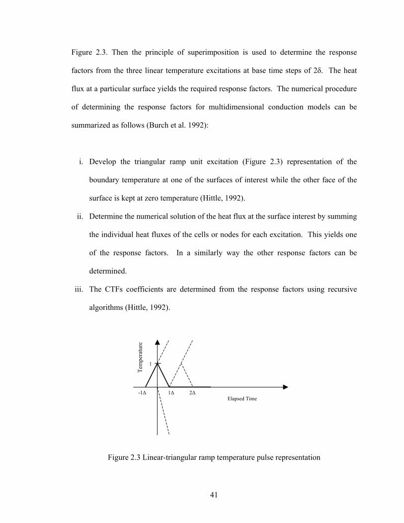
41
Figure 2.3. Then the principle of superimposition is used to determine the response
factors from the three linear temperature excitations at base time steps of 2δ. The heat
flux at a particular surface yields the required response factors. The numerical procedure
of determining the response factors for multidimensional conduction models can be
summarized as follows (Burch et al. 1992):
i. Develop the triangular ramp unit excitation (Figure 2.3) representation of the
boundary temperature at one of the surfaces of interest while the other face of the
surface is kept at zero temperature (Hittle, 1992).
ii. Determine the numerical solution of the heat flux at the surface interest by summing
the individual heat fluxes of the cells or nodes for each excitation. This yields one
of the response factors. In a similarly way the other response factors can be
determined.
iii. The CTFs coefficients are determined from the response factors using recursive
algorithms (Hittle, 1992).
-1∆ 1∆ 2∆Elapsed Time
Tem
pera
ture
1
Figure 2.3 Linear-triangular ramp temperature pulse representation
42
The Burch et al. (1992) finite difference procedure based CTF coefficients determination
method requires a separate standalone transient heat conduction analysis program with a
spatial discretization scheme. Thus, the Burch et al. method is difficult to be integrate
into existing building energy analysis and load calculation programs without significant
modifications of their codes (Burch et al. 1992).
Equivalent Wall Method
Kossecka (1998) and Carpenter et al. (2003a) developed the concept of an equivalent
wall, which replicates multi-dimensional thermal dynamics of the complex composite
wall with a simple homogeneous layer wall. The generated equivalent wall, which has
the same dynamic behavior to that of the real composite wall, is represented by one-
dimensional response factors or conduction transfer function that can be implemented in
the commonly used building energy analysis and load calculation programs (Kosny and
Kossecka 2002). Generating equivalent walls requires proper identification of the thermal
mass and negligible mass resistance components from the construction layer
configuration. The thermal characterization of constructions can be defined by a
parameter called thermal structure factor (Kossecka 1998). The concept of thermal
structure factor is presented next.
Thermal Structure Factors
Thermal structure factors, which are dimensionless parameters, define the thermal energy
storage characteristic of building structures when it goes through two successive steady
state ambient temperature transitions (Kossecka 1998; Kossecka and Kosny 2002).
43
Thermal structure factors of a wall depend on the resistance and thermal capacities of the
layers and their sequence of arrangements in the wall. Thermal structure factors (φ) of
building structures (Carpenter et al. 2003a; Kossecka 1998; Kossecka and Kosny 2002)
are given by:
( ) dxcC
L
pii2
0
11 θρϕ −= ∫ (2.9)
( )dxcC
L
pie θθρϕ −= ∫ 11
0
(2.10)
dxcC
L
pee2
0
1 θρϕ ∫= (2.11)
Besides, the following identity needs to be met by the thermal structure factors
12 =++ eeieii ϕϕϕ (2.12)
Where
C Overall thermal capacity of the wall, (J/m2 K)
cp specific heat of a layer in the wall, (J/kg K)
ρ density of a layer in the wall, (kg/m3)
L thickness of the wall, (m)
θ dimensionless temperature, (-)
φii Interior structure factor (-)
φie core structure factor (-)
44
φee exterior structure factor (-)
A high interior thermal structure factor (φii) implies that the higher thermal mass layer is
located near the interior surface and most of the resistance is located near the exterior
surface of the wall. Vice versa, a high exterior thermal structure factor (φee) indicates that
the higher thermal mass layer is located near the exterior surface and most of the
resistance is located near the interior surface of the wall. And a high core thermal
structure factor (φie) implies that the higher thermal mass layers are located at the center
of the wall and the resistances are placed symmetrically on both sides of the wall. The
relationships between response factors and thermal structure factors (Carpenter et al.
2003a; Kossecka 1998; Kossecka and Kosny 2002) are given:
iin
n CnX ϕδ −=∑∞
=1 (2.13)
ien
n CnY ϕδ =∑∞
=1 (2.14)
een
n CnZ ϕδ −=∑∞
=1 (2.15)
Where
Xn: the nth term exterior self-coupling response factor, (W/m2 K)
Yn: the nth term cross coupling response factor, (W/m2 K)
Zn: the nth term interior self-coupling response factor, (W/m2 K)
C Overall thermal capacity of the wall, (J/m2 K)
45
φii Interior structural factor (-)
φie core structural factor (-)
φee exterior structural factor (-)
δ time step, (s)
Equivalent wall Generation Procedure
The equivalent wall generation requires five steps (Carpenter et al. 2003a). These steps
are summarized as follows:
(1) Develop a three-dimensional model of the building envelope to exact dimensions
using multi-dimensional dimensional heat conduction solver computer programs.
(2) Generate three-dimensional response factors using numerical methods and use
them to determine the three dimensional conduction transfer function;
(3) Calculate the thermal structure factors of the composite wall using the three
dimensional response factors determined in step 2 and the thermal structure factor
identity;
(4) Generate the fictitious equivalent wall. The equivalent wall generation requires
selecting random set of resistances for each layers of the wall and calculating the
capacitance or randomly specifying the capacitance and calculating the
resistances. A three layer fictitious wall is recommended for simplicity
(Carpenter et al. 2003a). The material layer configuration, i.e., the relative
position of the high thermal mass and the high resistance layers in the fictitious
wall layers configuration must resemble that of the actual wall.
46
(5) The transfer function coefficients for the three-dimensional numerical model and
the equivalent wall model matching is done by trial-and-error until reasonable
accuracy is achieved by adjusting the resistance and/or capacitance of the
equivalent wall layers. The steady state resistance, thermal response factors and
structure factors of the real wall and the fictitious equivalent wall must be the
same.
State Space Method
The state space method can be used to determine conduction transfer function
coefficients that can represent multidimensional transient heat conduction in walls. The
state space method is based on first order differential equation representation of transient
heat conduction by spatially discretizing the conduction domain and representing the
inputs by continuous, piecewise linear functions (Seem 1987). The advantage of the state
space method compared to the Laplace transform method (Hittle, 1992) is that it can be
extended to solve multidimensional transient heat conduction problems. The state space
method is represented in the form of equations as follows:
[ ][ ] [ ][ ]bii TBTA
dtdT
+=
(2.16)
[ ] [ ][ ] [ ][ ]bTDTCq += (2.17)
Where
Ti vector of n interior node temperatures as state variables, °C (°F)
47
A a constant coefficient transition matrix with size of nxn
t the time, (s)
B the constant coefficient matrix of input vector of size (nxp)
Tb vector of p boundary temperatures as inputs, °C(°F)
q vector of p heat fluxes as outputs, W/m2°K(Btu/h⋅ft2⋅°F)
C a constant coefficient matrix of the output vectors of size (mxn)
D constant coefficients matrix of the input vector of size (mxp)
Solution of equations 2.16 and 2.17 for constant elements matrix of A and B in a compact
representation is given by:
( )∑ ∑=
=
=
=−− −=
nj
j
nj
jjtjjtjt qFTSq
0 1δδ (2.18)
Where
Sj are the conduction transfer function coefficients, (W/m2 K)
Fj are the coefficients of the past heat flux history terms, (-)
Two-dimensional state space method
Seem (1987) demonstrated that the state space method can be applied to model multi-
dimensional transient heat conduction in building envelopes. In the state space method,
the heat conduction domain is discretized in multi-dimensions; hence, the multi-
dimensional heat conduction effects in composite walls such as those with steel studs can
48
be modeled accurately. Therefore, the state space method can model dynamics of walls;
however, as the conduction domain becomes complex, the number of nodes required for
accurate modeling also increases. Consequently, evaluation of the exponential matrix
becomes cumbersome or sometimes almost impossible (Amjad et al. 2003).
Barrier to Use of Dynamic Multi-dimensional Models
Three multidimensional dynamic thermal bridge models, which could be integrated into
existing one-dimensional conduction transfer function procedures, have been proposed.
The multidimensional dynamic CTF models are: the equivalent wall method, the state
space method, and the numerical CTF method. Beyond other reasons, implementation
and integration of these models into the existing programs has been delayed due to
inherent limitations in the development of the multi-dimensional dynamic procedures,
and high computational resource requirement. These barriers to implementation in whole
building load calculation / energy simulation programs include:
The equivalent wall and the Burch et al., numerical CTF models require either
separate standalone multidimensional transient heat conduction analysis
numerical programs or integration of a significant multi-dimensional conduction
subprogram.
Models with spatial discretization requirements need both an implementation of
the discretization procedure and user interface to support this level of details.
Given the complexity of providing an interface to specify a whole building, this
may be too much of a refinement.

49
The equivalent wall method thermo-physical properties determined by trial-and-
error could be out of range for typical building materials properties.
Although the state space method does not require a separate standalone numerical
program, a spatial discretization tool is necessary. On the other hand, the state
space method can be integrated with existing building energy analysis and load
calculation programs most conveniently if an automatic building envelope
discretization and/or interactive user interface for material specification and
construction model reduction program is made available. However, the multi-
dimensional state space method will suffer from a numerical accuracy problem
that grows as the number of nodes increases.

50
51
CHAPTER III
3. Radiant Time Series Method Improvements
This chapter covers several improvements to the Radiant Time Series Method (RTSM).
These improvements include: new algorithm for generating Radiant Time Factors (RTF)
and developing a one-dimensional finite volume numerical method periodic response
factor generating procedure, adapting an improved fenestration model and establishing
radiative / convective splits, developing a procedure for accounting heat losses through
fenestration to the outside, and facilitating implementation of the RTSM procedure in
different computation environments.
There are several approaches for generating the RTF for a given building zone. Since
these procedures have been adopted directly or indirectly from a full-blown heat balance
method (HBM) procedure, they tend to have some unnecessary overhead and a simpler
method developed specifically for RTF generation is highly desirable. Derivation of the
reduced HBM RTF engine is described in Section 3.1. The new radiant time factors
(RTF) generating algorithm utilizes periodic response factors (PRF) to model transient
conduction as described in Section 3.1.1. Currently available PRF generation procedures
convert conduction transfer function coefficients generated using Laplace and State
Space method.
52
This procedure is undesirable for use in VBA and SCILAB type computational
environments. Therefore, a one-dimensional finite volume numerical procedure for
computing periodic response factors has been implemented and investigated. The finite
volume numerical procedure implementation is discussed in Section 3.1.2. Derivation of
the algorithm and validations are given in APPENDIX-B.
As part of this research, an improved fenestration model compatible with currently
available fenestration data will be adapted to the RTSM. Furthermore, a new set of
radiative / convective splits compatible with the improved fenestration model has been
established. The improvement in the RTSM fenestration model is described in Section
3.2.
The previously published RTSM cooling load procedure2 (Rees et al. 2000a; Spitler et al.
1997) does not account for the solar and internal radiant heat gains conducted back out of
the zone. Ignoring these back losses is the principal reason that the RTSM over predicts
the peak-cooling load. An approximate algorithm that accounts for zone radiant loss in
the RTSM procedure has been derived and is described in Section 3.3.
For all improvements described in this section, results and discussed are provided for
each Sections. However, for improvement to the fenestration model and the heat losses
accounting procedure, it is highly desirable to demonstrate satisfactory performance over
a wider range of cases. Such a study is the subject of Chapter 4.
2 Referred to as the “original RTSM procedure” in this thesis.

53
3.1 New RTF Calculation Engine
The Radiant Time Series Method (RTSM) converts the radiant component of the heat
gains into cooling loads using the Radiant Time Factors (RTF), a 24-term series. The 24
hourly radiant time factors describe the dynamic response characteristics of a zone. Two
procedures were developed for RTF generation (Spitler et al. 1997). Currently there are
five approaches available for generating the radiant time factors: (1) software that comes
with the book Cooling and Heating Load Calculation Principles (Pedersen et al. 1998),
(2) software that comes with the book by McQuiston et al. (2005), (3) software developed
as based on the ASHRAE toolkit (Iu 2001), (4) tabulated RTF values in the ASHRAE
Handbook of Fundamentals, and (5) RTF generated from zone heat gain weighting
factors. The first four approaches use the full heat balance method as a calculation
engine to compute the RTFs. The HBM programs that come with the books by Pedersen
et al. and McQuiston et al. are limited to twelve surfaces only for any zone and the RTF
generating software developed by Iu is limited to six surfaces. The McQuiston et al. and
Pedersen, et al. programs are full load calculation programs that treat the RTF as an
auxiliary output. The McQuiston et al. and Iu programs have interfaces that allow users
to select material layer thermo-physical properties from a database. The interface used
by McQuiston et al. accepts much more information than is actually necessary to generate
the RTF. The tabulated values in the Handbook of Fundamentals were generated for
limited building design conditions using Pedersen et al. program. But the accuracy of the
RTSM peak cooling load resulting from the users choosing the “nearest” zone has not
been investigated.
54
An alternative approach (Spitler and Fisher 1999b) is to generate radiant time factors
directly from a set of zone heat gain weighting factors using the existing ASHRAE 472-
RP database (Sowell 1988a; Sowell 1988b; Sowell 1988c). These weighting factors were
developed for use with the Transfer Function Method (TFM). This approach would use a
computer program to map a given zone to the fourteen zone parameters in the database
and transform the weighting factors to radiant time factors using matrix manipulation.
However, the 472-RP weighting factors do not represent all possible zone designs and
construction types. ASHRAE’s 472-RP weighting factors were generated for
combination of discrete building design parameters; hence, the RTF generated from these
weighting factors represent only specific buildings. User judgment is required to match
an existing building to one of the combinations of discrete building design parameters.
In conclusion, the existing approaches all suffer from being too cumbersome, requiring
too much user judgment, or too limited with regard to the number of zones surfaces.
Therefore, development of an RTF coefficient-generating tool that handles a wide range
of practical design conditions is desirable. Such a tool should meet the following
requirements:
i. capable of generating RTF for a wide variety of practical building
constructions, including a practical number of building surfaces, i.e. more
than twelve.
ii. simple user interface that does not require unnecessary information.
iii. can be integrated with other applications such as spreadsheets by
eliminating unnecessary features and source code. It would be preferable to
55
minimize the required calculations and eliminate the use of DLLs if
possible.
iv. The methodology should take advantage of the steady periodic nature of the
boundary condition. When this is done, the methodology can benefit from
matrix algebra easily accessed in modern computing languages and
environments such as SCILAB or MATLAB.
The new RTF calculation engine is derived from an inside surface heat balance and room
air heat balance for adiabatic zone. The simplified procedure eliminates several steps of
the HBM, particularly the exterior surface heat balance and eliminates input data that are
not necessary for the RTF generation. The new RTF generating program is first
developed as a FORTRAN DLL which may be called from a spreadsheet. Then, it will
be implemented in VBA and SCILAB. The following section describes the derivation of
the mathematical algorithm for the RTF generation program.
3.1.1 The Mathematical Model -Reduced Heat Balance Method
The formulation of the mathematical model for the radiant time factor generating
procedure makes use of the major assumptions used in the Heat Balance Method (HBM)
(Pedersen et al. 1997); that surfaces (walls, roofs, windows, etc) can be treated as having
uniform surface temperatures, uniform long wave and short wave length radiation;
surfaces are gray; one-dimensional conduction is valid and surfaces are exposed to steady
periodic boundary conditions. The simplified heat balance procedure for RTF generation
uses an inside surface heat balance, steady periodic boundary condition, constant
56
convection coefficients and constant room air temperature. The simplified HB procedure
for RTF generation eliminates the following procedures that are part of the full heat
balance method: outside surface heat balance, weather data, solar radiation calculations,
shading calculations, infiltration and ventilation. Because this simplified version of the
HBM uses a smaller number of heat balance steps, it will be referred to here as the
“Reduced Heat Balance Method” (RHBM). In the next section, the RHBM is described
step-by-step.
The inside surface heat balance for the ith surface is given by:
0'',
'',
'',
'', =+++ igainiradicondiconv qqqq &&&& (3.1)
Where,
'',iconvq& = convection heat flux from the room air to the ith surface, Btu/h⋅ft2
(W/m2)
'',icondq& = the ith surface conduction heat flux from the outside surface to the inside
surface, Btu/h⋅ft2 (W/m2)
'',iradq& = radiant heat flux from other internal surfaces to the ith surface, Btu/h⋅ft2
(W/m2)
'',igainq& = radiant heat gain flux of the ith surface from lights, people and
equipments, Btu/h⋅ft2 (W/m2)
57
Conduction Model
The RTSM uses air-to-air periodic response factors to compute conduction heat gain
driven by steady periodic exterior sol-air temperature and a constant indoor air
temperature. For RTF generation, surface-to-surface periodic response factors are used
with steady periodic surface temperatures computed with the reduced heat balance
method. The transient conduction heat flux at the inside surface using surface periodic
response factors (Spitler et al. 1997) for steady periodic boundary conditions is given by:
∑∑=
−=
− −=23
0,,
23
0,,
'',,
jjtiInPj
jjtiOutPjticond TZTYq δδ& (3.2)
Where,
δjtiInT −,, = inside surface temperature jth hours before the current hour, °F (°C)
δjtiOutT −,, = outside surface temperature jth hours before the current hour, °F (°C)
PjY = surface-to-surface cross periodic response factor, Btu/h⋅ft2⋅°F (W/m2⋅°C)
PjZ = surface-to-surface inside periodic response factor, Btu/h⋅ft2⋅°F (W/m2⋅°C)
The transient heat conduction equation can be simplified further using the appropriate
boundary conditions.
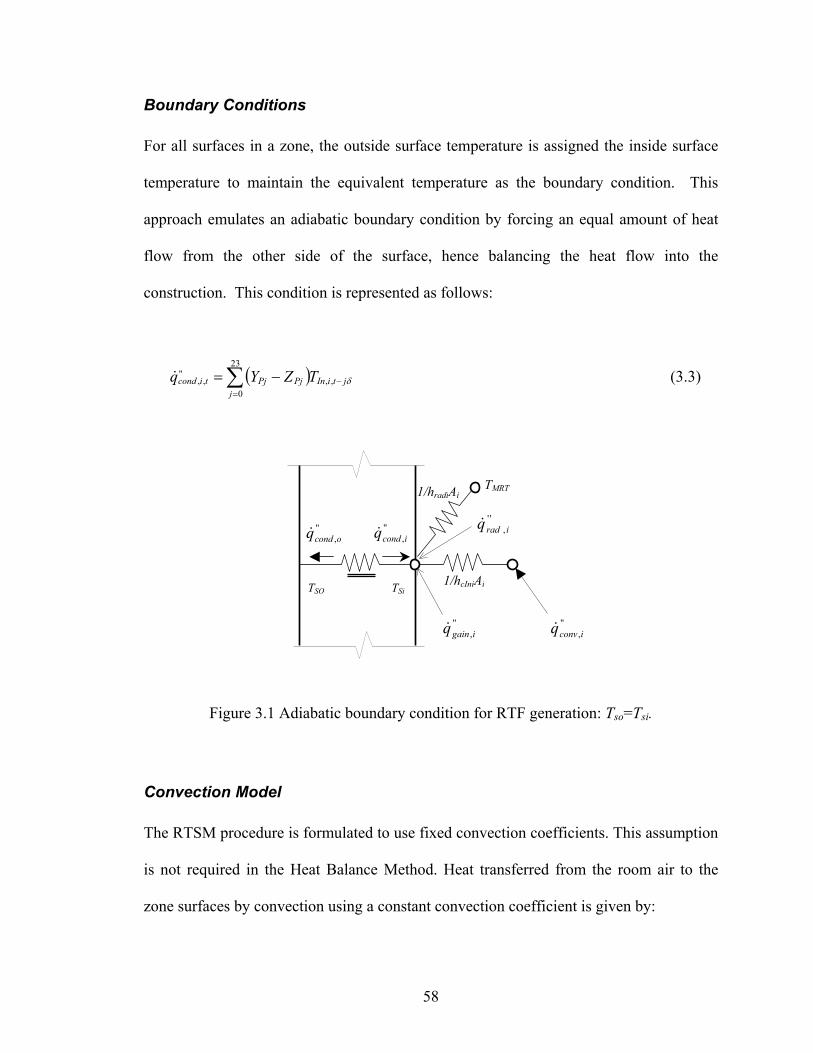
58
Boundary Conditions
For all surfaces in a zone, the outside surface temperature is assigned the inside surface
temperature to maintain the equivalent temperature as the boundary condition. This
approach emulates an adiabatic boundary condition by forcing an equal amount of heat
flow from the other side of the surface, hence balancing the heat flow into the
construction. This condition is represented as follows:
( )∑=
−−=23
0,,
'',,
jjtiInPjPjticond TZYq δ& (3.3)
Figure 3.1 Adiabatic boundary condition f
Convection Model
The RTSM procedure is formulated to use fixed con
is not required in the Heat Balance Method. Heat
zone surfaces by convection using a constant convec
TSO
T
TSi
i
'',icondq&
'',igainq&
'',ocondq&
TMR
'', iradq&
1/hcIniAi
1/hradiA
''q&
or RTF ge
vection co
transferre
tion coeff
neration: Tso=Tsi.
efficients. This assumption
d from the room air to the
icient is given by:
,iconv
59
( )tiInricInticonv TThq ,,,''
,, −=& (3.4)
Where,
tiInT ,, = inside temperature of the ith surface at time t, °F (°C)
rT = constant room air temperature, °F (°C)
icInh , = convection coefficient of the ith inside surface, Btu/h⋅ft2⋅oF (W/m2 °C)
'',, ticonvq& = convection heat flux at the ith surface at time t, Btu/h⋅ft2 (W/m2)
Internal Longwave Radiation Model
The internal long wave radiation model assumes zone air is transparent to long wave
radiation and considers the zone surfaces as gray and the long wavelength radiation as
diffuse. With these assumptions, long wavelength radiation in building can be modeled
using the uniform radiosity method, the total gray exchange factors method (Hottel and
Sarofim 1967), the mean radiant temperature and balance (MRT/balance) method
(Walton 1980) or the Mean Radiant Temperature Network (MRTNet) method (Carroll
1980).
The uniform radiosity and the total gray exchange factor method require exact view
factors. The uniform radiosity method involves solving the radiosity at every time step
hence the method is computationally intensive, which makes it unsuitable for building
applications. The total gray exchange factor method combines the surface properties and
geometries into the gray exchange factors, which can be computed at the beginning of the
60
simulation and eliminates the simultaneous solution at every time step. However, it
requires exact view factors. In real buildings, calculation of exact view factors is
computationally intensive and the furnishings and other internal heat sources cannot be
easily represented and are mobile during the lifetime of the buildings. Hence, any gains in
accuracy facilitated using the exact view factors are unlikely to be realized in practice.
Therefore, the extra effort introduced in specifying locations and dimensions of
furnishings is unlikely to be rewarded with any tangible benefit.
The advantage of the MRT/ balance and MRTNet methods is that both use approximate
view factors based on area and emissivity and allow an approximate representation of
furnishings and partitions surfaces. In the MRT/balance method each surface exchanges
radiation with a fictitious mean radiant temperature calculated from area-emissivity-
surface temperature product weighted of the remaining surfaces viewed by the surface.
The radiation flux imbalance resulting from approximate view factors in the
MRT/balance method is balanced by redistributing it to the surfaces.
In the MRTNet method each surface exchanges radiation with a single fictitious mean
radiant temperature of the zone that is computed from all surfaces. The radiation
coefficient linking the each surface is corrected for each surface depending on the surface
and MRT temperature of the zone and hence balances the zone radiation exchange. Both
MRT methods essentially have the same accuracy (Liesen and Pedersen, 1997).
Therefore, due to simplicity, the mean radiant temperature network (MRTNet) method
(Carroll 1980) has been selected for use in the RTF generation algorithm. With the
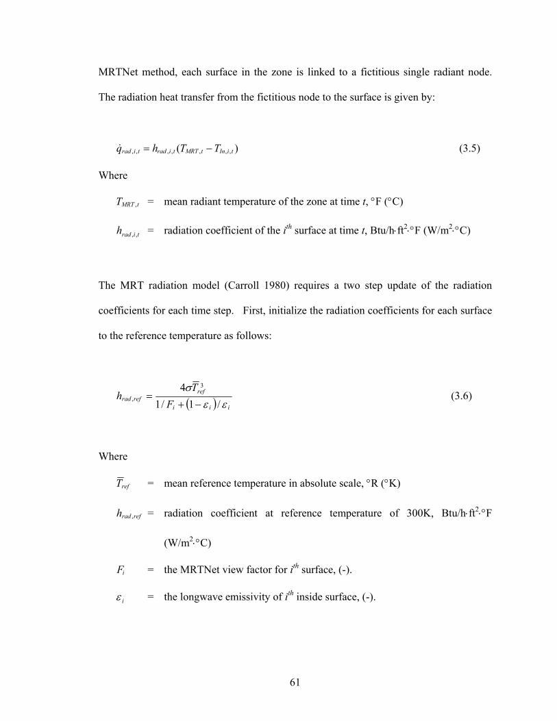
61
MRTNet method, each surface in the zone is linked to a fictitious single radiant node.
The radiation heat transfer from the fictitious node to the surface is given by:
)( ,,,,,,, tiIntMRTtiradtirad TThq −=& (3.5)
Where
tMRTT , = mean radiant temperature of the zone at time t, °F (°C)
tiradh ,, = radiation coefficient of the ith surface at time t, Btu/h⋅ft2⋅°F (W/m2⋅°C)
The MRT radiation model (Carroll 1980) requires a two step update of the radiation
coefficients for each time step. First, initialize the radiation coefficients for each surface
to the reference temperature as follows:
( ) iii
refrefrad F
Th
εεσ
/1/14 3
,−+
= (3.6)
Where
refT = mean reference temperature in absolute scale, °R (°K)
refradh , = radiation coefficient at reference temperature of 300K, Btu/h⋅ft2⋅°F
(W/m2⋅°C)
iF = the MRTNet view factor for ith surface, (-).
iε = the longwave emissivity of ith inside surface, (-).
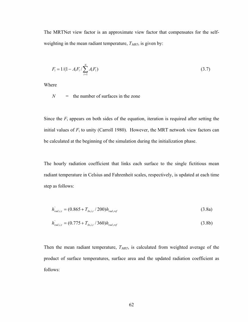
62
The MRTNet view factor is an approximate view factor that compensates for the self-
weighting in the mean radiant temperature, TMRT, is given by:
)/1/(11
∑=
−=N
iiiiii FAFAF (3.7)
Where
N = the number of surfaces in the zone
Since the Fi appears on both sides of the equation, iteration is required after setting the
initial values of Fi to unity (Carroll 1980). However, the MRT network view factors can
be calculated at the beginning of the simulation during the initialization phase.
The hourly radiation coefficient that links each surface to the single fictitious mean
radiant temperature in Celsius and Fahrenheit scales, respectively, is updated at each time
step as follows:
refradtiIntirad hTh ,,,'
,, )200/865.0( += (3.8a)
refradtiIntirad hTh ,,,'
,, )360/775.0( += (3.8b)
Then the mean radiant temperature, TMRT, is calculated from weighted average of the
product of surface temperatures, surface area and the updated radiation coefficient as
follows:

63
∑∑==
=N
itiraditiIn
N
itiraditMRT hAThAT
1
',,,,
1,,
', / (3.9)
Again the radiation coefficients are adjusted using the updated mean radiant temperature
in Celsius and Fahrenheit scales, respectively, as follows:
',,
',,, )200/865.0( tiradtMRTtirad hTh += (3.10a)
',,
',,, )360/775.0( tiradtMRTtirad hTh += (3.10b)
Then the corrected radiation coefficient of the individual surface is used to compute the
room mean radiant temperature (TMRT,t) as follows:
∑∑==
=N
itiraditiIn
N
itiraditMRT hAThAT
1,,,,
1,,, / (3.11)
So, for each iteration of the heat balance, a fixed two-step iteration to determine the
radiation coefficient and the MRT is done as given in Equations 3.7 to 3.11.
Radiant Heat Gain Distribution Model
Computing the precise distribution of long-wave radiation from internal sources requires
knowledge of the exact location / position, surface area and temperature of the sources.
This approach creates additional complexity to internal radiation exchange models.
Therefore, the conventional approach is to distribute the internal radiant heat gains
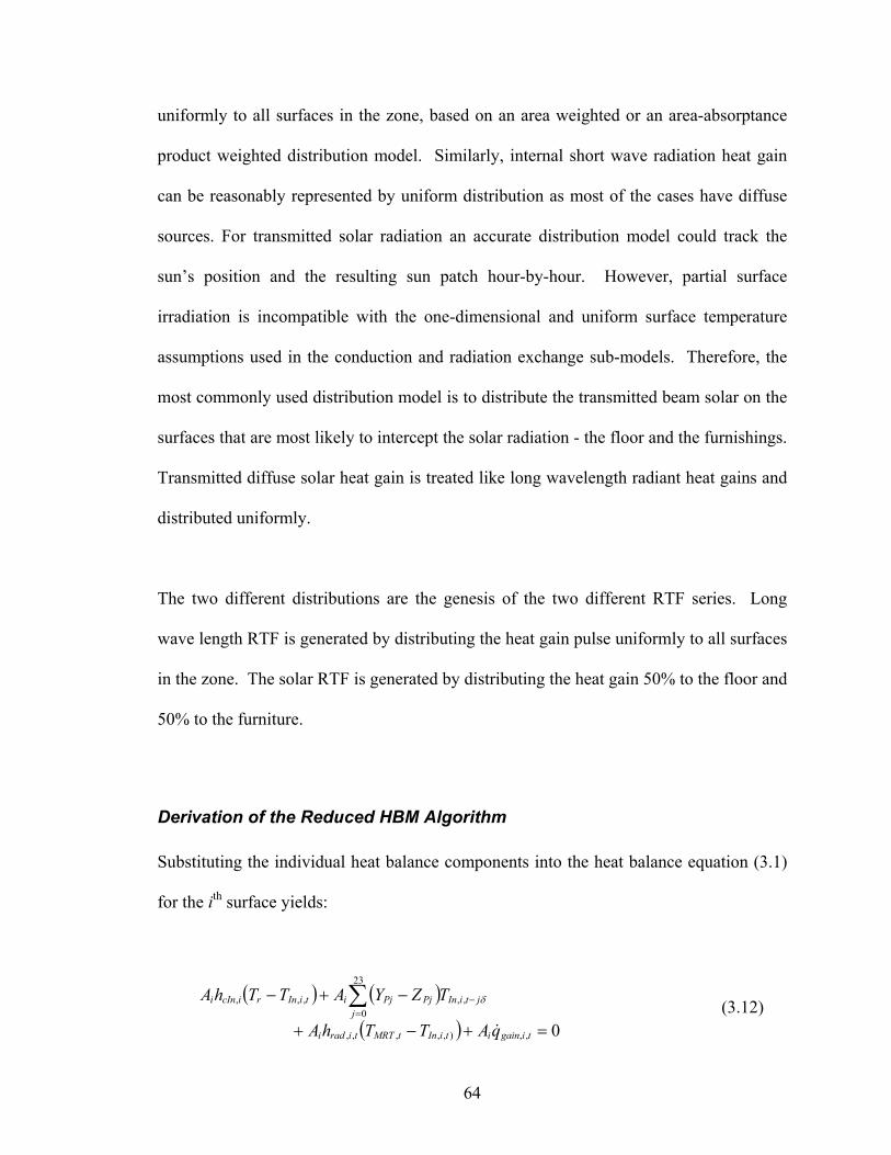
64
uniformly to all surfaces in the zone, based on an area weighted or an area-absorptance
product weighted distribution model. Similarly, internal short wave radiation heat gain
can be reasonably represented by uniform distribution as most of the cases have diffuse
sources. For transmitted solar radiation an accurate distribution model could track the
sun’s position and the resulting sun patch hour-by-hour. However, partial surface
irradiation is incompatible with the one-dimensional and uniform surface temperature
assumptions used in the conduction and radiation exchange sub-models. Therefore, the
most commonly used distribution model is to distribute the transmitted beam solar on the
surfaces that are most likely to intercept the solar radiation - the floor and the furnishings.
Transmitted diffuse solar heat gain is treated like long wavelength radiant heat gains and
distributed uniformly.
The two different distributions are the genesis of the two different RTF series. Long
wave length RTF is generated by distributing the heat gain pulse uniformly to all surfaces
in the zone. The solar RTF is generated by distributing the heat gain 50% to the floor and
50% to the furniture.
Derivation of the Reduced HBM Algorithm
Substituting the individual heat balance components into the heat balance equation (3.1)
for the ith surface yields:
( ) ( )( ) 0,,),,,,,
23
0,,,,,
=+−+
−+− ∑=
−
tigainitiIntMRTtiradi
jjtiInPjPjitiInricIni
qATThA
TZYATThA
&
δ (3.12)
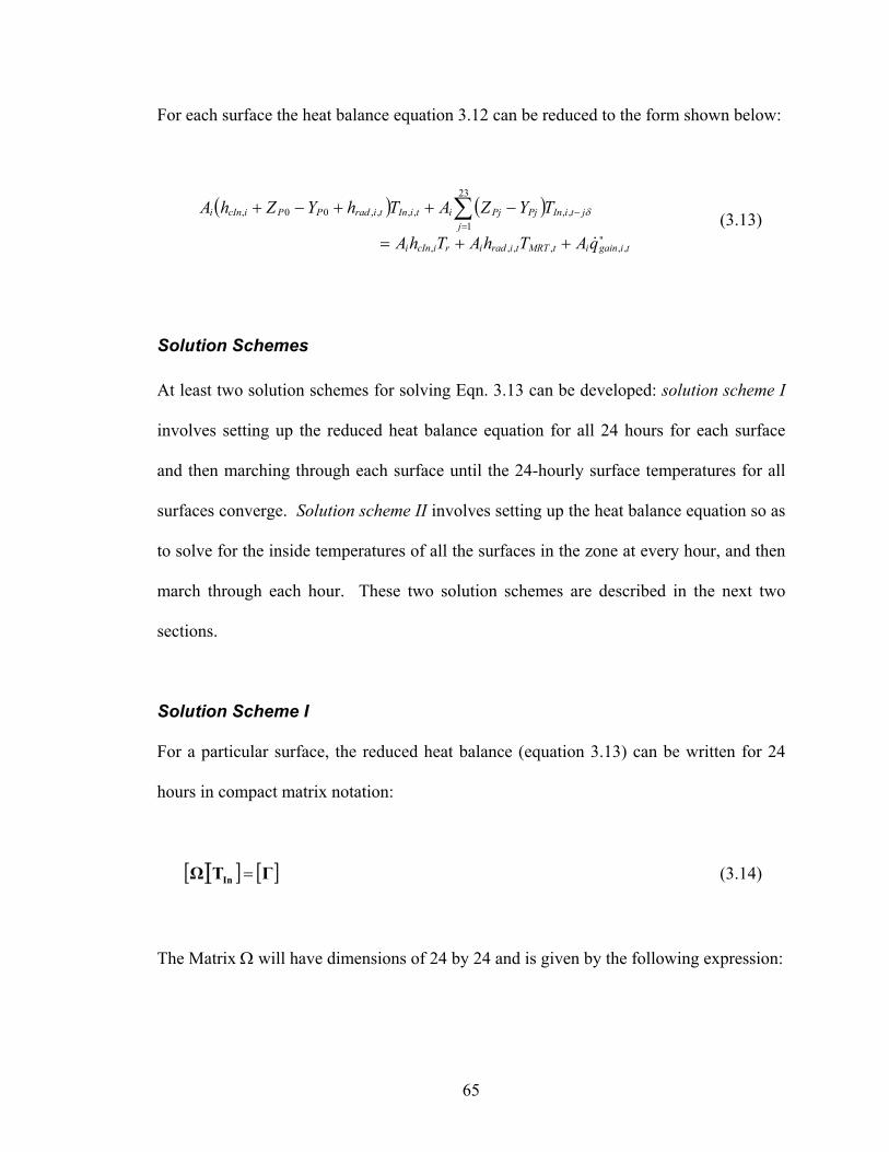
65
For each surface the heat balance equation 3.12 can be reduced to the form shown below:
( ) ( )''
,,,,,,
23
1,,,,,,00,
tigainitMRTtiradiricIni
jjtiInPjPjitiIntiradPPicIni
qAThAThA
TYZAThYZhA
&++=
−++−+ ∑=
− δ (3.13)
Solution Schemes
At least two solution schemes for solving Eqn. 3.13 can be developed: solution scheme I
involves setting up the reduced heat balance equation for all 24 hours for each surface
and then marching through each surface until the 24-hourly surface temperatures for all
surfaces converge. Solution scheme II involves setting up the heat balance equation so as
to solve for the inside temperatures of all the surfaces in the zone at every hour, and then
march through each hour. These two solution schemes are described in the next two
sections.
Solution Scheme I
For a particular surface, the reduced heat balance (equation 3.13) can be written for 24
hours in compact matrix notation:
[ ][ ] [ ]ΓTΩ In = (3.14)
The Matrix Ω will have dimensions of 24 by 24 and is given by the following expression:
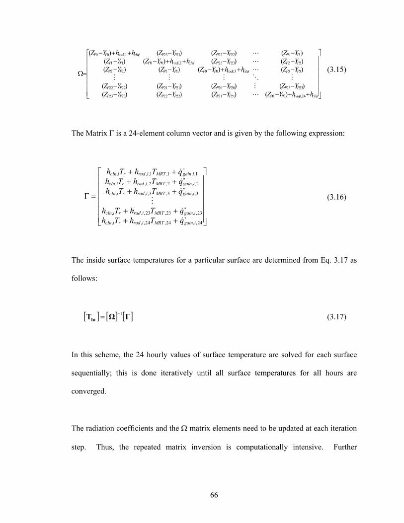
66
++−−−−−−−−
−++−−−−−++−−−−−++−
=Ω
icIniradPPPPPPPP
PPPPPPPP
PPicIniradPPPPPP
PPPPicIniradPPPP
PPPPPPicIniradPP
hhYZYZYZYZYZYZYZYZ
YZhhYZYZYZYZYZhhYZYZYZYZYZhhYZ
,24,,00212122222323
2323202021212222
33,3,,001122
222323,2,,0011
1122222323,1,,00
)()()()()()()()(
)()()()()()()()()()()()(
LM
MOMMMLLL
(3.15)
The Matrix Γ is a 24-element column vector and is given by the following expression:
++++
++++++
=Γ
''24,,24,24,,,
''23,,23,23,,,
''3,,3,3,,,
''2,,2,2,,,
''1,,1,1,,,
igainMRTiradricIn
igainMRTiradricIn
igainMRTiradricIn
igainMRTiradricIn
igainMRTiradricIn
qThThqThTh
qThThqThThqThTh
&&
M&&&
(3.16)
The inside surface temperatures for a particular surface are determined from Eq. 3.17 as
follows:
[ ] [ ] [ ]ΓΩTIn1−= (3.17)
In this scheme, the 24 hourly values of surface temperature are solved for each surface
sequentially; this is done iteratively until all surface temperatures for all hours are
converged.
The radiation coefficients and the Ω matrix elements need to be updated at each iteration
step. Thus, the repeated matrix inversion is computationally intensive. Further
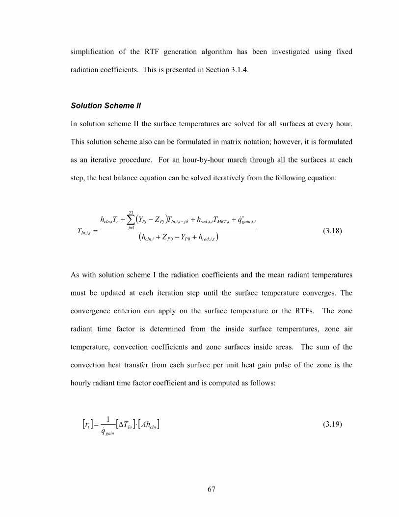
67
simplification of the RTF generation algorithm has been investigated using fixed
radiation coefficients. This is presented in Section 3.1.4.
Solution Scheme II
In solution scheme II the surface temperatures are solved for all surfaces at every hour.
This solution scheme also can be formulated in matrix notation; however, it is formulated
as an iterative procedure. For an hour-by-hour march through all the surfaces at each
step, the heat balance equation can be solved iteratively from the following equation:
( )
( )tiradPPicIn
tigaintMRTtiradj
jtiInPjPjricIn
tiIn hYZh
qThTZYThT
,,00,
'',,,,,
23
1,,,
,,+−+
++−+=
∑=
− &δ
(3.18)
As with solution scheme I the radiation coefficients and the mean radiant temperatures
must be updated at each iteration step until the surface temperature converges. The
convergence criterion can apply on the surface temperature or the RTFs. The zone
radiant time factor is determined from the inside surface temperatures, zone air
temperature, convection coefficients and zone surfaces inside areas. The sum of the
convection heat transfer from each surface per unit heat gain pulse of the zone is the
hourly radiant time factor coefficient and is computed as follows:
[ ] [ ] [ ]cInIngain
t AhTq
r ⋅∆=&
1 (3.19)
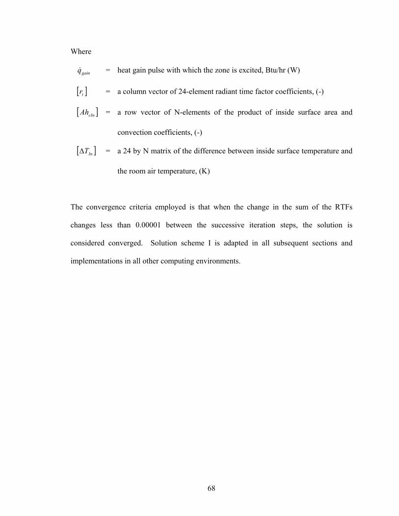
68
Where
gainq& = heat gain pulse with which the zone is excited, Btu/hr (W)
[ ]tr = a column vector of 24-element radiant time factor coefficients, (-)
[ ]cInAh = a row vector of N-elements of the product of inside surface area and
convection coefficients, (-)
[ ]InT∆ = a 24 by N matrix of the difference between inside surface temperature and
the room air temperature, (K)
The convergence criteria employed is that when the change in the sum of the RTFs
changes less than 0.00001 between the successive iteration steps, the solution is
considered converged. Solution scheme I is adapted in all subsequent sections and
implementations in all other computing environments.
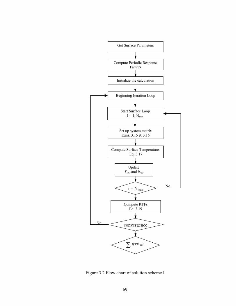
Figure 3.2 Flo
Get Surface Parameters
C
Compute Periodic Response Factors
Initialize the calculation
Beginning Iteration Loop
Start Surface Loop I = 1, Nmax
Set up system matrix Eqns. 3.15 & 3.16
ompute Surface TemperaturesEq. 3.17
i = Nmax
Compute RTFs Eq. 3.19
No
Update TMRT and hrad
No
69
w chart of solution scheme I
∑ =1RTF
convergence
70
3.1.2 Validation of the New RTF Engine
The new RTF generating engine has been validated against the full-blown heat balance
method FORTRAN program originally developed by Pedersen et al. (1997). The test
zone geometry and construction fabrics are given in Table 3.1. Three construction types:
light, medium and heavy weight constructions were used for the validation. Each zone
has a single exterior surface with single pane clear glass and 50% glazing fraction of the
exterior facade. Zones were modeled with and without carpeting.
Table 3.1 Description of test zone constructions for RTF generation algorithm validation Fabric Element Lightweight Mediumweight Heavyweight
External wall steel siding, 2 in insulation, air space, ¾ in gypsum
4in face brick, 2 in insulation, air space, ¾ in gypsum
4in face brick, air space 2 in. insulation, 8 in HW concrete, ¾ in gypsum
Roof/Ceiling 4 in. LW concrete, ceiling air space, acoustic tile
4 in. HW concrete, ceiling air space, acoustic tile
8 in. HW concrete, ceiling air space, acoustic tile
Partition ¾ in. gyp, air space, ¾.in. gypsum
¾ in. gyp, air space, 3/4.in. gypsum
¾ in. gyp, 8 in. HW concrete block, 3/4.in. gypsum
Floor Acoustic tile, ceiling air space, 4 in. LW concrete
Acoustic tile, ceiling air space, 4 in. HW concrete
Acoustic tile, ceiling air space, 8 in. HW concrete
Furnishing 1 in. wood @ 50% of floor area
1 in. wood @ 50% of floor area
1 in. wood @ 50% of floor area
Carpeting Resistance layer of 2.73 ft2 h ºF/Btu
Resistance layer of 2.73 ft2 h ºF/Btu
Resistance layer of 2.73 ft2 h ºF/Btu
Notes: 1. Surface layers are listed in order from the outside of the room to the inside of the room. 2. The test zone is 15ft x 30ft x 9ft high. The test zone has one exterior wall, 30 ft long. 3. The % glazing is fraction of the exterior facade. 4. Long wavelength absorptance of 0.9 were used for all inside surfaces
The following two heat gain pulse distribution models were used for the RTF generation:
(1) area weighted uniform distribution model for non-solar RTF, and (2) for the solar-
RTF generation 50% to the floor and 50% to the thermal mass surfaces. The RTF plots
are shown in Figures 3.3 to 3.6. The RTF plots for medium and heavyweight
construction zones are shown in Appendix A. Root mean square errors (RMSE) of the
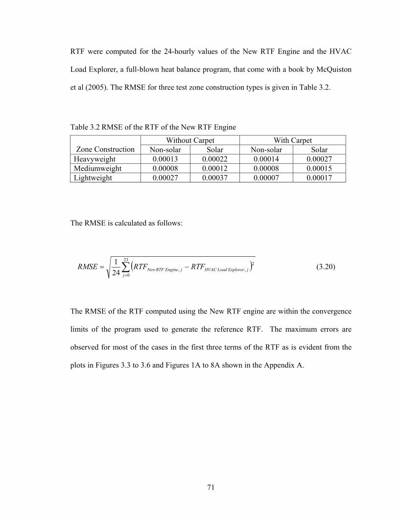
71
RTF were computed for the 24-hourly values of the New RTF Engine and the HVAC
Load Explorer, a full-blown heat balance program, that come with a book by McQuiston
et al (2005). The RMSE for three test zone construction types is given in Table 3.2.
Table 3.2 RMSE of the RTF of the New RTF Engine
Without Carpet With Carpet Zone Construction Non-solar Solar Non-solar Solar
Heavyweight 0.00013 0.00022 0.00014 0.00027 Mediumweight 0.00008 0.00012 0.00008 0.00015 Lightweight 0.00027 0.00037 0.00007 0.00017
The RMSE is calculated as follows:
( )∑=
−=23
0
2,,24
1j
jExplorerLoadHVACjEngineRTFNew RTFRTFRMSE (3.20)
The RMSE of the RTF computed using the New RTF engine are within the convergence
limits of the program used to generate the reference RTF. The maximum errors are
observed for most of the cases in the first three terms of the RTF as is evident from the
plots in Figures 3.3 to 3.6 and Figures 1A to 8A shown in the Appendix A.
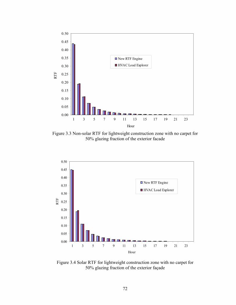
72
0.00
0.05
0.10
0.15
0.20
0.25
0.30
0.35
0.40
0.45
0.50
1 3 5 7 9 11 13 15 17 19 21 23
Hour
RTF
New RTF Engine
HVAC Load Explorer
Figure 3.3 Non-solar RTF for lightweight construction zone with no carpet for
50% glazing fraction of the exterior facade
0.00
0.05
0.10
0.15
0.20
0.25
0.30
0.35
0.40
0.45
0.50
1 3 5 7 9 11 13 15 17 19 21 23
Hour
RTF
New RTF Engine
HVAC Load Explorer
Figure 3.4 Solar RTF for lightweight construction zone with no carpet for
50% glazing fraction of the exterior façade
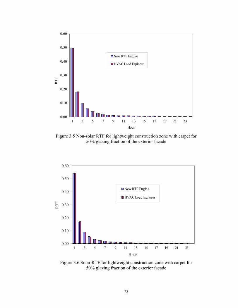
73
0.00
0.10
0.20
0.30
0.40
0.50
0.60
1 3 5 7 9 11 13 15 17 19 21 23
Hour
RTF
New RTF Engine
HVAC Load Explorer
Figure 3.5 Non-solar RTF for lightweight construction zone with carpet for
50% glazing fraction of the exterior facade
0.00
0.10
0.20
0.30
0.40
0.50
0.60
1 3 5 7 9 11 13 15 17 19 21 23
Hour
RTF
New RTF Engine
HVAC Load Explorer
Figure 3.6 Solar RTF for lightweight construction zone with carpet for
50% glazing fraction of the exterior facade
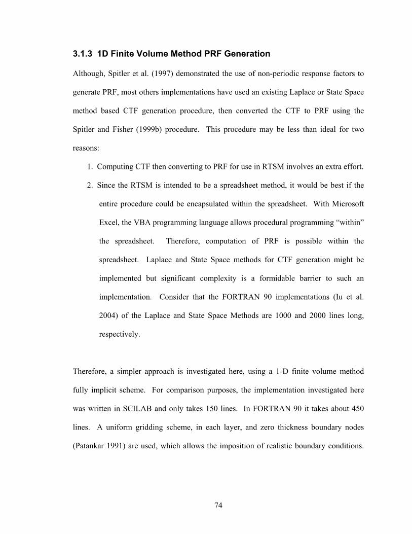
74
3.1.3 1D Finite Volume Method PRF Generation
Although, Spitler et al. (1997) demonstrated the use of non-periodic response factors to
generate PRF, most others implementations have used an existing Laplace or State Space
method based CTF generation procedure, then converted the CTF to PRF using the
Spitler and Fisher (1999b) procedure. This procedure may be less than ideal for two
reasons:
1. Computing CTF then converting to PRF for use in RTSM involves an extra effort.
2. Since the RTSM is intended to be a spreadsheet method, it would be best if the
entire procedure could be encapsulated within the spreadsheet. With Microsoft
Excel, the VBA programming language allows procedural programming “within”
the spreadsheet. Therefore, computation of PRF is possible within the
spreadsheet. Laplace and State Space methods for CTF generation might be
implemented but significant complexity is a formidable barrier to such an
implementation. Consider that the FORTRAN 90 implementations (Iu et al.
2004) of the Laplace and State Space Methods are 1000 and 2000 lines long,
respectively.
Therefore, a simpler approach is investigated here, using a 1-D finite volume method
fully implicit scheme. For comparison purposes, the implementation investigated here
was written in SCILAB and only takes 150 lines. In FORTRAN 90 it takes about 450
lines. A uniform gridding scheme, in each layer, and zero thickness boundary nodes
(Patankar 1991) are used, which allows the imposition of realistic boundary conditions.
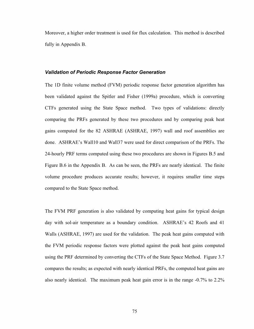
75
Moreover, a higher order treatment is used for flux calculation. This method is described
fully in Appendix B.
Validation of Periodic Response Factor Generation
The 1D finite volume method (FVM) periodic response factor generation algorithm has
been validated against the Spitler and Fisher (1999a) procedure, which is converting
CTFs generated using the State Space method. Two types of validations: directly
comparing the PRFs generated by these two procedures and by comparing peak heat
gains computed for the 82 ASHRAE (ASHRAE, 1997) wall and roof assemblies are
done. ASHRAE’s Wall10 and Wall37 were used for direct comparison of the PRFs. The
24-hourly PRF terms computed using these two procedures are shown in Figures B.5 and
Figure B.6 in the Appendix B. As can be seen, the PRFs are nearly identical. The finite
volume procedure produces accurate results; however, it requires smaller time steps
compared to the State Space method.
The FVM PRF generation is also validated by computing heat gains for typical design
day with sol-air temperature as a boundary condition. ASHRAE’s 42 Roofs and 41
Walls (ASHRAE, 1997) are used for the validation. The peak heat gains computed with
the FVM periodic response factors were plotted against the peak heat gains computed
using the PRF determined by converting the CTFs of the State Space Method. Figure 3.7
compares the results; as expected with nearly identical PRFs, the computed heat gains are
also nearly identical. The maximum peak heat gain error is in the range -0.7% to 2.2%
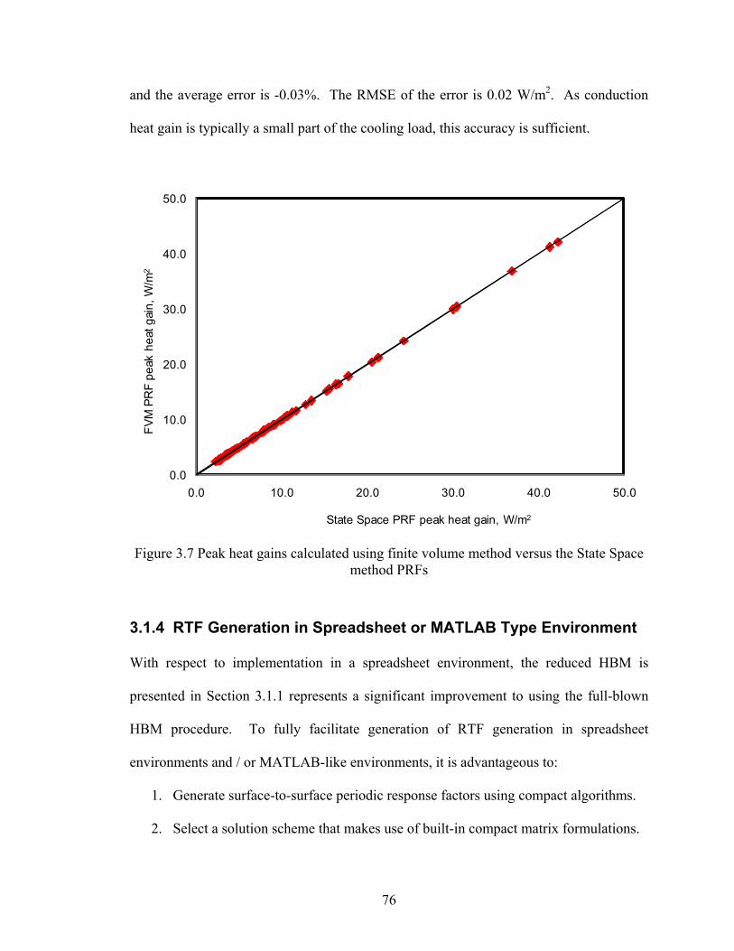
76
and the average error is -0.03%. The RMSE of the error is 0.02 W/m2. As conduction
heat gain is typically a small part of the cooling load, this accuracy is sufficient.
0.0
10.0
20.0
30.0
40.0
50.0
0.0 10.0 20.0 30.0 40.0 50.0
FVM
PR
F pe
ak h
eat g
ain,
W/m
2
State Space PRF peak heat gain, W/m2
Figure 3.7 Peak heat gains calculated using finite volume method versus the State Space
method PRFs
3.1.4 RTF Generation in Spreadsheet or MATLAB Type Environment
With respect to implementation in a spreadsheet environment, the reduced HBM is
presented in Section 3.1.1 represents a significant improvement to using the full-blown
HBM procedure. To fully facilitate generation of RTF generation in spreadsheet
environments and / or MATLAB-like environments, it is advantageous to:
1. Generate surface-to-surface periodic response factors using compact algorithms.
2. Select a solution scheme that makes use of built-in compact matrix formulations.
77
3. Investigate the use of constant radiation coefficient with the intention of reducing
the computational effort.
The RTF generation algorithm has also been implemented in the SCILAB programming
environment to take advantage of the built-in compact matrix algebra. The
implementation has been demonstrated successfully. The algorithm reads the periodic
response factors from a text input file and uses 146 lines of code to generate the RTF.
The SCILAB code for the RTF generation is given Appendix B.
The RTF generation implementation in VBA has been validated against a full-blown heat
balance method program results using six test zones based on light, medium and heavy
construction in Table 3.1 with and without carpets. The RMSE of the RTF generated
using the VBA program compared to the full-blown heat balance method program varied
in the range from 0.0002 to 0.003. The RTF should sum to one. The RTF generated with
the VBA program sum within 0.000001 of one. For the SCILAB case, the RTF sum to
within 0.00001 of one. The RMSE of the RTF generated in SCILAB compared to full-
blown heat balance method is in the range from 0.0008 to 0.0044. These errors are
within the convergence limits of the RTF sum.
The RTF generation algorithm described in Section 3.1.1 requires repeated matrix
inversions and/or iterations; hence it is computationally intensive. The RTF generation
procedure can be formulated with an approximation using a constant radiation
coefficient, calculated with Eq. 3.6 at the reference temperature and never corrected. The
78
constant radiation coefficient avoids the system matrix update at every iteration and
thereby reduces the computational time by about one-half compared to a variable
radiation coefficient. Appendix C shows a few cases where this approximation has been
compared to more detailed approaches (i.e. with variable radiation coefficient) and it
gives nearly identical results. For the three cases, the hourly cooling load error computed
in VBA by using constant radiation coefficients was less than 0.02 Btu/hr⋅ft2 or the error
was in the range -0.04% to 0.0% of the peak load. Further validation is recommended for
this simplification.
3.2 Improved Fenestration Model
The radiant time series method (RTSM) was originally developed for use with shading
coefficients and double-strength glass angular properties for computing solar heat gain
through fenestration glazing systems. There have been new developments in glazing
system data and fenestration models made available since the RTSM was first introduced.
Solar heat gain can be computed with solar heat gain coefficients that effectively replace
shading coefficients and data published by window manufacturers and ASHRAE are in
the form of solar heat gain coefficient (SHGC) rather than shading coefficients. The
RTSM cooling load calculation procedure needs to adapt these developments. Therefore,
one of the objectives of this thesis is to adapt a fenestration model for the RTSM
procedure3 that makes use of the recent developments and new fenestration data.
3 After adapting the fenestration models and the associated radiative/convective splits, the RTSM is referred to as the “current RTSM procedure”.
79
The improved fenestration model is covered in four sections: development of improved
fenestration model, parametric investigation of radiative / convective splits for
fenestrations conduction and solar heat gains, application of fenestration model without
interior shades, and application of fenestration models with interior shade. Section 3.2.1
deals with development of the improved fenestration models and discusses the challenge
of the application of the improved model due to lack of complete window manufacturer’s
data. Parametric investigation to determine radiative / convective splits for conduction
and solar heat gains is discussed in Section 3.2.2. Applications of the improved
fenestration model for glazing without and with interior shade are discussed in Sections
3.2.3 and 3.2.4, respectively.
3.2.1 Development of Improved Fenestration Model
The fenestration model used for the RTSM is kept simple as it is intended for a simplified
load calculation procedure. The fenestration model proposed for the RTSM uses the
solar heat gain coefficient (SHGC) and interior attenuation coefficient (IAC) (ASHRAE
2001; ASHRAE 2005). The IAC accounts for the attenuation of solar heat gain by
interior shading device. The SHGC is a property of the glazing system that combines the
transmittance and the inward flow fraction of the absorbed solar radiation. The RTSM
treats the radiant fraction of the absorbed component of solar heat gains using non-solar
radiant time factors. The fenestration model requires angle dependent SHGC. The
SHGC combines the transmitted and absorbed components of solar heat gain that needs
to be treated separately. Different approaches that require angle dependent SHGC and
transmittances have been investigated to develop procedures for computing the absorbed
80
component of solar heat gains. These approaches did not seem to maintain the simplicity
required and at the same time required more input data than available. However, window
manufacturers usually provide normal solar heat gain coefficient, normal visible
transmittance, and U-value of the glazing system. Therefore, a fenestration class
procedure that uses normal solar heat gain coefficient and tabulated angular correction
method originally developed by Barnaby et al. (2005) has been proposed to overcome the
problem of lack of angle dependent SHGC. The fenestration model adopted for the
RTSM requires the following input parameters:
1. Normal beam SHGC
2. Diffuse SHGC
3. Angular Correction
4. Interior attenuation coefficient (IAC)
5. Radiative / Convective splits
The radiative / convective split is required to account for the treatment of the absorbed
component and its importance is more important for glazing with interior shades as
discussed in Section 3.2.2. The solar heat gain through a glazing system without internal
shading device (ASHRAE 2005) is given by:
drdNDSHG SHGCEESHGCEq ⋅++⋅⋅= )()(cos'' θθ& (3.21)
where
''SHGq& = total solar heat gain, Btu/h⋅ft2 (W/m2)
81
θ = angle of incidence between the sun’s rays and normal to the surface,
radian
NDE = normal direct irradiation, Btu/h⋅ft2 (W/m2)
dE = diffuse irradiation from the sky, Btu/h⋅ft2 (W/m2)
rE = diffuse irradiation reflected from the ground or other surfaces, Btu/h⋅ft2
(W/m2)
)(θSHGC = beam solar heat gain coefficient, (-)
dSHGC = diffuse solar heat gain coefficient, (-)
The solar heat gain for a fenestration system with interior shading devices (ASHRAE
2005) is given by:
[ ] IACSHGCEESHGCEq drdDNSHG ⋅⋅++⋅⋅= )()(cos'' θθ& (3.22)
Where,
IAC = interior attenuation coefficient, (-)
The solar heat gain calculated with Eqns. 3.21 and 3.22 includes transmitted radiation and
radiation absorbed by the windows or shades that flows into the space. In the original
RTSM cooling load calculation procedure the transmitted components are assumed 100%
radiant while the absorbed component is composed of radiative and convective fractions.
The original RTSM procedure uses a 63%/37% radiative / convective split for the
absorbed component of solar heat gain (Spitler et al. 1997) for fenestration without
82
interior shades. The challenge for practicing engineers is that window manufacturers
usually do not provide all input data required by fenestration models. Determination of
radiative / convective splits for conduction and solar heat gains of fenestration is
discussed in detail in Section 3.2.2. In the absence of angular dependent SHGC mapping
procedures proposed by Barnaby et al. (2005) can be introduced. The proposed mapping
procedure is presented next.
Mapping Manufacturer’s Windows
Window manufacturers usually provide the solar heat gain coefficients and visible
transmittance at normal incident angle and overall U-value of the fenestration system.
ASHRAE (2005) provides angle dependent solar heat gain coefficients, transmittance and
absorptance of glazing systems but this data set is not linked to specific manufacturer’s
window. The challenge is how to map between the manufacturer’s windows and the
tabulated ASHRAE’s angle-dependent data.
The proposed mapping procedure is as follows:
• Start with manufacturer’s normal solar heat gain coefficient, visible transmittance
and U-value.
• Selecting a tabulated set of optical properties of glazing system data for which
normal SHGC is nearest to the manufacturer’s normal SHGC and visible
transmittance based on type of glazing (e.g. clear glass, tinted glass, low-e,
reflective coating, number of panes, and thickness of the glass panes).
83
• Correct the SHGC of the tabulated values using the ratio of normal SHGC given
by the manufacturers to the tabulated normal SHGC value. This step provides
approximate beam and diffuse SHGC for the manufacturer’s window.
The mapping procedure can reasonably duplicate the angular dependent solar heat gain
coefficient; however, the transmittance and absorptance of a glazing system cannot be
mapped explicitly since different combinations of the latter two optical properties can
produce the same solar heat gain coefficient. The absorbed component of solar heat gain
for several glazing systems has been computed from tabulated optical properties and is
shown in Figure 3.8. The absorbed component is a small fraction of the solar heat gain
for single and double pane clear glazing systems. But it could be as high as 40% for low-
e and coated multiple pane glazing systems. For instance, for the high performance green
tinted triple pane glazing system (29c) shown in Figure 3.8, the absorbed fraction is as
high as 38% for incident angles up to 40°.
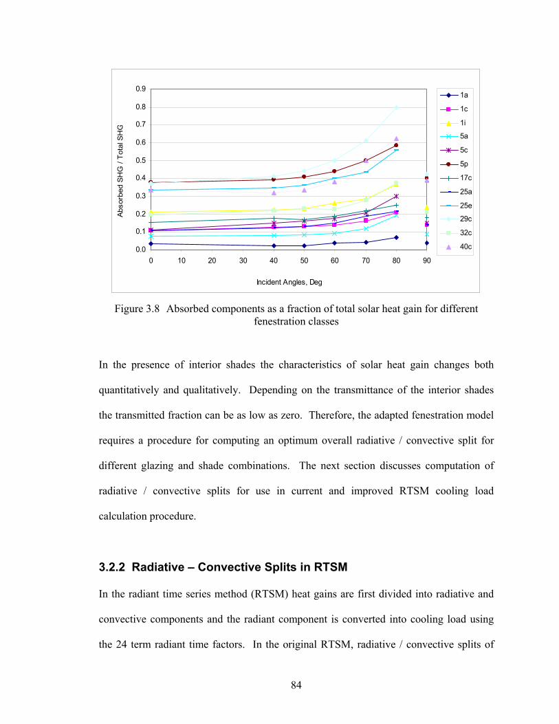
84
0.0
0.1
0.2
0.3
0.4
0.5
0.6
0.7
0.8
0.9
0 10 20 30 40 50 60 70 80 90
Incident Angles, Deg
Abs
orbe
d S
HG
/ To
tal S
HG
1a
1c
1i
5a
5c
5p
17c
25a
25e
29c
32c
40c
Figure 3.8 Absorbed components as a fraction of total solar heat gain for different
fenestration classes
In the presence of interior shades the characteristics of solar heat gain changes both
quantitatively and qualitatively. Depending on the transmittance of the interior shades
the transmitted fraction can be as low as zero. Therefore, the adapted fenestration model
requires a procedure for computing an optimum overall radiative / convective split for
different glazing and shade combinations. The next section discusses computation of
radiative / convective splits for use in current and improved RTSM cooling load
calculation procedure.
3.2.2 Radiative – Convective Splits in RTSM
In the radiant time series method (RTSM) heat gains are first divided into radiative and
convective components and the radiant component is converted into cooling load using
the 24 term radiant time factors. In the original RTSM, radiative / convective splits of
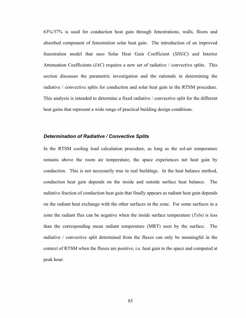
85
63%/37% is used for conduction heat gain through fenestrations, walls, floors and
absorbed component of fenestration solar heat gain. The introduction of an improved
fenestration model that uses Solar Heat Gain Coefficient (SHGC) and Interior
Attenuation Coefficients (IAC) requires a new set of radiative / convective splits. This
section discusses the parametric investigation and the rationale in determining the
radiative / convective splits for conduction and solar heat gain in the RTSM procedure.
This analysis is intended to determine a fixed radiative / convective split for the different
heat gains that represent a wide range of practical building design conditions.
Determination of Radiative / Convective Splits
In the RTSM cooling load calculation procedure, as long as the sol-air temperature
remains above the room air temperature, the space experiences net heat gain by
conduction. This is not necessarily true in real buildings. In the heat balance method,
conduction heat gain depends on the inside and outside surface heat balance. The
radiative fraction of conduction heat gain that finally appears as radiant heat gain depends
on the radiant heat exchange with the other surfaces in the zone. For some surfaces in a
zone the radiant flux can be negative when the inside surface temperature (TsIn) is less
than the corresponding mean radiant temperature (MRT) seen by the surface. The
radiative / convective split determined from the fluxes can only be meaningful in the
context of RTSM when the fluxes are positive, i.e. heat gain to the space and computed at
peak hour.
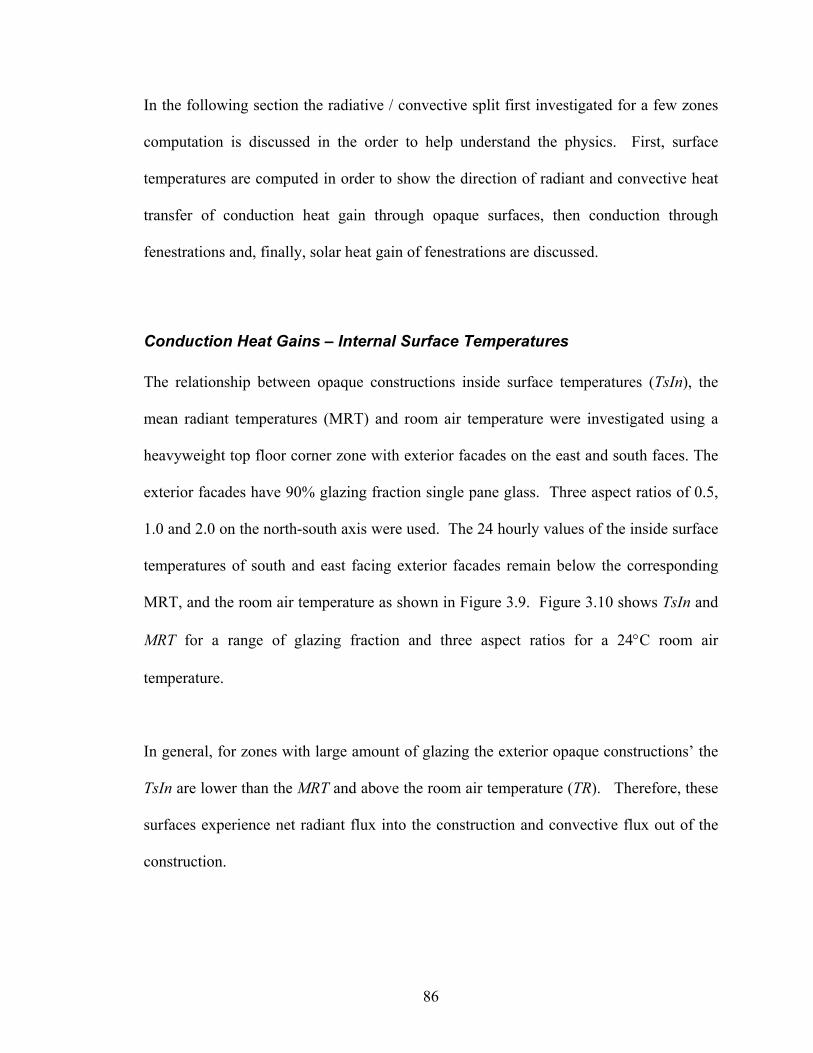
86
In the following section the radiative / convective split first investigated for a few zones
computation is discussed in the order to help understand the physics. First, surface
temperatures are computed in order to show the direction of radiant and convective heat
transfer of conduction heat gain through opaque surfaces, then conduction through
fenestrations and, finally, solar heat gain of fenestrations are discussed.
Conduction Heat Gains – Internal Surface Temperatures
The relationship between opaque constructions inside surface temperatures (TsIn), the
mean radiant temperatures (MRT) and room air temperature were investigated using a
heavyweight top floor corner zone with exterior facades on the east and south faces. The
exterior facades have 90% glazing fraction single pane glass. Three aspect ratios of 0.5,
1.0 and 2.0 on the north-south axis were used. The 24 hourly values of the inside surface
temperatures of south and east facing exterior facades remain below the corresponding
MRT, and the room air temperature as shown in Figure 3.9. Figure 3.10 shows TsIn and
MRT for a range of glazing fraction and three aspect ratios for a 24°C room air
temperature.
In general, for zones with large amount of glazing the exterior opaque constructions’ the
TsIn are lower than the MRT and above the room air temperature (TR). Therefore, these
surfaces experience net radiant flux into the construction and convective flux out of the
construction.
87
0
5
10
15
20
25
30
35
40
0 4 8 12 16 20 24
Hours
Tem
pera
ture
s,o C
South Wall TsIn South Wall TmrtEast Wall TsIn East Wall Tmrt
Figure 3.9 TsIn and MRT of heavyweight construction opaque exterior surfaces and 24°C room air temperature
The above analysis would suggest that the radiative fraction should be zero or even
negative for cases with high solar or internal heat gains. However, there are cases
without high solar or internal heat gains, e.g. warehouses, for which the radiation fraction
should have a positive value.
88
10
15
20
25
30
35
40
45
0 0.1 0.2 0.3 0.4 0.5 0.6 0.7 0.8 0.9
Exterior Facade Glazing Fraction
Tem
pera
ture
, o C
South Wall TsIn
South Wall MRT
Figure 3.10 TsIn and the corresponding MRT for opaque surface at peak load for three
aspect ratios and 24°C room air temperature
Zones with high solar heat gains (zones with large single and double pane clear glass or
high solar heat gain coefficient) result in closely similar inside surface temperatures that
reduce the net radiant heat exchange with fenestration. Hence the radiant fraction for
conduction heat gains in a zone with a large amount of solar and internal radiant heat
gains tends to be lower.
This quandary can be resolved by understanding that, for zones with high solar and
internal heat gains, the contributions of exterior opaque construction conduction heat
gains to the peak cooling load is small. Hence the peak cooling load is not sensitive to
radiative / convective splits of conduction heat gains through walls and roofs for these
zones, as a small fraction of the total cooling load. Then the question becomes what
value of radiative / convective split gives an accurate cooling load over a wide range of
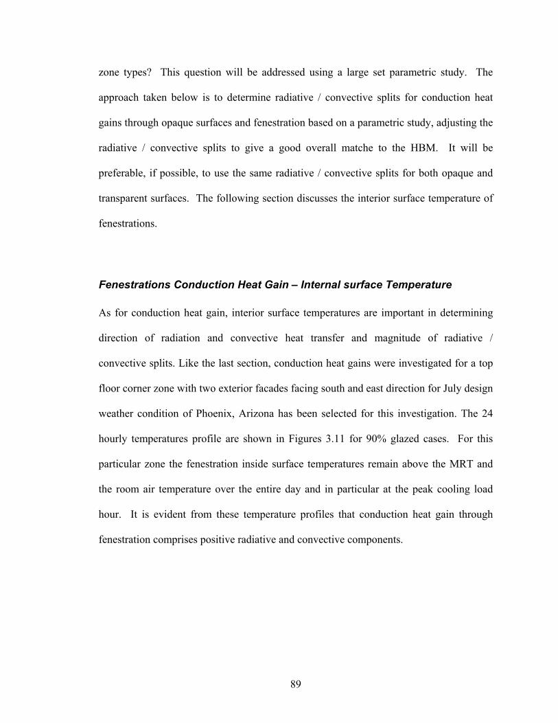
89
zone types? This question will be addressed using a large set parametric study. The
approach taken below is to determine radiative / convective splits for conduction heat
gains through opaque surfaces and fenestration based on a parametric study, adjusting the
radiative / convective splits to give a good overall matche to the HBM. It will be
preferable, if possible, to use the same radiative / convective splits for both opaque and
transparent surfaces. The following section discusses the interior surface temperature of
fenestrations.
Fenestrations Conduction Heat Gain – Internal surface Temperature
As for conduction heat gain, interior surface temperatures are important in determining
direction of radiation and convective heat transfer and magnitude of radiative /
convective splits. Like the last section, conduction heat gains were investigated for a top
floor corner zone with two exterior facades facing south and east direction for July design
weather condition of Phoenix, Arizona has been selected for this investigation. The 24
hourly temperatures profile are shown in Figures 3.11 for 90% glazed cases. For this
particular zone the fenestration inside surface temperatures remain above the MRT and
the room air temperature over the entire day and in particular at the peak cooling load
hour. It is evident from these temperature profiles that conduction heat gain through
fenestration comprises positive radiative and convective components.
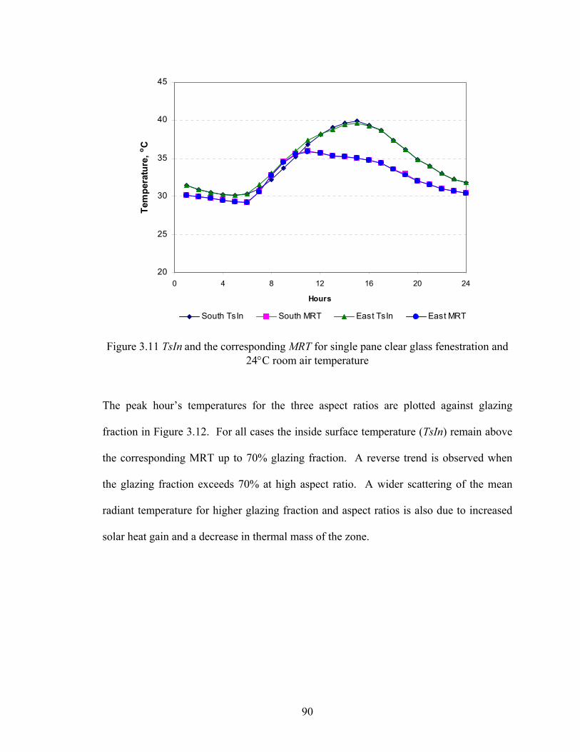
90
20
25
30
35
40
45
0 4 8 12 16 20 24
Hours
Tem
pera
ture
,o C
South TsIn South MRT East TsIn East MRT
Figure 3.11 TsIn and the corresponding MRT for single pane clear glass fenestration and
24°C room air temperature
The peak hour’s temperatures for the three aspect ratios are plotted against glazing
fraction in Figure 3.12. For all cases the inside surface temperature (TsIn) remain above
the corresponding MRT up to 70% glazing fraction. A reverse trend is observed when
the glazing fraction exceeds 70% at high aspect ratio. A wider scattering of the mean
radiant temperature for higher glazing fraction and aspect ratios is also due to increased
solar heat gain and a decrease in thermal mass of the zone.
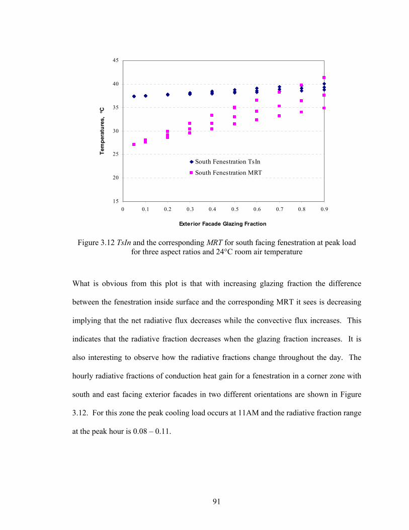
91
15
20
25
30
35
40
45
0 0.1 0.2 0.3 0.4 0.5 0.6 0.7 0.8 0.9
Exterior Facade Glazing Fraction
Tem
pera
ture
s,o C
South Fenestration TsIn
South Fenestration MRT
Figure 3.12 TsIn and the corresponding MRT for south facing fenestration at peak load
for three aspect ratios and 24°C room air temperature
What is obvious from this plot is that with increasing glazing fraction the difference
between the fenestration inside surface and the corresponding MRT it sees is decreasing
implying that the net radiative flux decreases while the convective flux increases. This
indicates that the radiative fraction decreases when the glazing fraction increases. It is
also interesting to observe how the radiative fractions change throughout the day. The
hourly radiative fractions of conduction heat gain for a fenestration in a corner zone with
south and east facing exterior facades in two different orientations are shown in Figure
3.12. For this zone the peak cooling load occurs at 11AM and the radiative fraction range
at the peak hour is 0.08 – 0.11.
92
0.0
0.1
0.2
0.3
0.4
0.5
0 4 8 12 16 20 24
Rad
iativ
e Fr
actio
n
HoursSouth Fenestration SEZ East Fenestration SEZSouth Fenestration SWZ West Fenestration SWZ
Figure 3.13 Radiative fractions for fenestration in a heavyweight construction zone with two exterior facades single pane clear glass with 90% glazing fraction
For the same building design, a zone with exterior surfaces on the south and west facades
with the peak cooling load occurring in the afternoon at 5PM, the radiative fraction lies
between 0.12 – 0.17. The radiative fraction varies hourly and is smaller when the
temperature differences between the inside surface temperature and its mean radiant
temperature is smaller. A similar hourly plot of the radiative fraction for 50% glazing
fraction of the exterior facade is shown in Figure 3.14. The radiative fraction for south-
east and south-west facing zones were found out to be in the range from 0.33 to 0.34 and
from 0.31 to 0.34, respectively. The increase in the radiant fraction with decrease in
glazing fraction is directly related to amount of solar heat gain and zone construction
fabric.
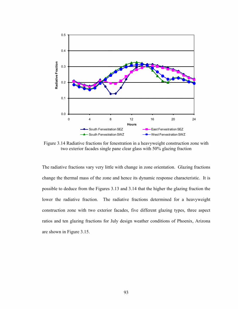
93
0.0
0.1
0.2
0.3
0.4
0.5
0 4 8 12 16 20 24
Rad
iativ
e Fr
actio
n
HoursSouth Fenestration SEZ East Fenestration SEZSouth Fenestration SWZ West Fenestration SWZ
Figure 3.14 Radiative fractions for fenestration in a heavyweight construction zone with two exterior facades single pane clear glass with 50% glazing fraction
The radiative fractions vary very little with change in zone orientation. Glazing fractions
change the thermal mass of the zone and hence its dynamic response characteristic. It is
possible to deduce from the Figures 3.13 and 3.14 that the higher the glazing fraction the
lower the radiative fraction. The radiative fractions determined for a heavyweight
construction zone with two exterior facades, five different glazing types, three aspect
ratios and ten glazing fractions for July design weather conditions of Phoenix, Arizona
are shown in Figure 3.15.
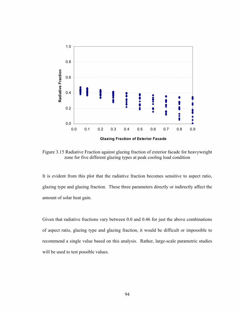
94
0.0
0.2
0.4
0.6
0.8
1.0
0.0 0.1 0.2 0.3 0.4 0.5 0.6 0.7 0.8 0.9
Glazing Fraction of Exterior Facade
Rad
iativ
e Fr
actio
n
Figure 3.15 Radiative Fraction against glazing fraction of exterior facade for heavyweight
zone for five different glazing types at peak cooling load condition
It is evident from this plot that the radiative fraction becomes sensitive to aspect ratio,
glazing type and glazing fraction. These three parameters directly or indirectly affect the
amount of solar heat gain.
Given that radiative fractions vary between 0.0 and 0.46 for just the above combinations
of aspect ratio, glazing type and glazing fraction, it would be difficult or impossible to
recommend a single value based on this analysis. Rather, large-scale parametric studies
will be used to test possible values.
95
Solar heat gains Radiative Convective Split
The use of solar heat gain coefficients (SHGC) and interior attenuation coefficients (IAC)
to compute fenestration solar heat gain for the RTSM requires introduction of radiant
fraction to estimate the convective and radiant components. The introduction of radiant
fraction is important to model fenestration with interior shades since the attenuation
coefficient accounts only for the reduction of solar heat gain but does not quantify the
change in radiative / convective split. Though the solar heat gain radiative / convective
split depend on different building design parameters, two types of preliminary
investigations were conducted - one for fenestration without interior shade and another
for fenestration with shade.
Fenestration without Internal Shade
For most glazing types the transmitted component, which is 100% radiant, is the largest
fraction of solar heat gain. The absorbed solar heat gain comprises radiant and
convective components. Taken together, the radiant fraction is the larger portion for
almost all unshaded glazing types. Since the original and current RTSM cooling load
calculation procedures do not account for the radiant heat loss by conduction, the
treatment of solar heat gain as 100% radiant doesn’t lead to under prediction of the peak
cooling load. The effect of this assumption has been investigated parametrically. This
assumption is not realistic for fenestration system with internal shades since a substantial
portion of solar heat gains can be convective. Detailed radiative / convective split
analysis over a wide range of building design conditions were conducted to determine the
optimum radiative fraction range and is presented in the following section.
96
Fenestration with Internal Shade
The fenestration model adopted for the RTSM uses the interior attenuation coefficients
(IAC) to account for the reduction of solar heat gain by interior shading devices.
ASHRAE provides tabulated IAC for different combination of glazing system and
interior shading devices (ASHRAE 2001; ASHRAE 2005). Interior shading devices have
two effects: first, reduction of solar heat gain, which is taken care by using the interior
attenuation coefficient; second, increase in the relative proportion of the absorbed
component. Therefore, the use of IAC accounts for the attenuation effect but not to
changes in the relative proportions of transmitted and absorbed components. The
absorbed solar heat gain change from short wave to long wave and the long wave
radiation exchange with the other surface in zone depends on the inside surface
temperatures, long wavelength emissivities and zone geometry.
In this investigation five different glass types were investigated: single pane clear glass,
double pane clear glass, two double pane low-e glasses, and double pane reflective coated
glass. The investigation included typical internal heat gains and the following building
design parameters: glazing types, glazing fractions, interior shades, construction fabrics
(light and heavyweight), furnishings thermal mass, aspect ratio, number of external
facades and zone orientations were varied. The radiative fractions representing a wide
range of building design conditions are shown in Figures 3.16 and 3.17.
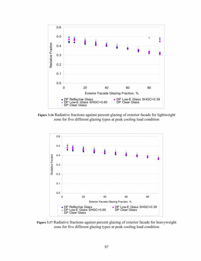
97
0.0
0.1
0.2
0.3
0.4
0.5
0.6
0 20 40 60 80
Exterior Facade Glazing Fraction, %
Radi
ative
Fra
ctio
n
DP Reflective Glass DP Low-E Glass SHGC=0.39DP Low-E Glass SHGC=0.65 DP Clear GlassSP Clear Glass
Figure 3.16 Radiative fractions against percent glazing of exterior facade for lightweight
zone for five different glazing types at peak cooling load condition
0.0
0.1
0.2
0.3
0.4
0.5
0.6
0 20 40 60 80
Exterior Facade Glazing Fraction, %
Rad
iativ
e Fr
actio
n
DP Reflective Glass DP Low-E Glass SHGC=0.39DP Low-E Glass SHGC=0.65 DP Clear GlassSP Clear Glass
Figure 3.17 Radiative fractions against percent glazing of exterior facade for heavyweight
zone for five different glazing types at peak cooling load condition
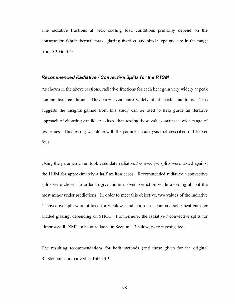
98
The radiative fractions at peak cooling load conditions primarily depend on the
construction fabric thermal mass, glazing fraction, and shade type and are in the range
from 0.30 to 0.53.
Recommended Radiative / Convective Splits for the RTSM
As shown in the above sections, radiative fractions for each heat gain vary widely at peak
cooling load condition. They vary even more widely at off-peak conditions. This
suggests the insights gained from this study can be used to help guide an iterative
approach of choosing candidate values, then testing these values against a wide range of
test zones. This testing was done with the parametric analysis tool described in Chapter
four.
Using the parametric run tool, candidate radiative / convective splits were tested against
the HBM for approximately a half million cases. Recommended radiative / convective
splits were chosen in order to give minimal over prediction while avoiding all but the
most minor under predictions. In order to meet this objective, two values of the radiative
/ convective split were utilized for window conduction heat gain and solar heat gain for
shaded glazing, depending on SHGC. Furthermore, the radiative / convective splits for
“Improved RTSM”, to be introduced in Section 3.3 below, were investigated.
The resulting recommendations for both methods (and those given for the original
RTSM) are summarized in Table 3.3.
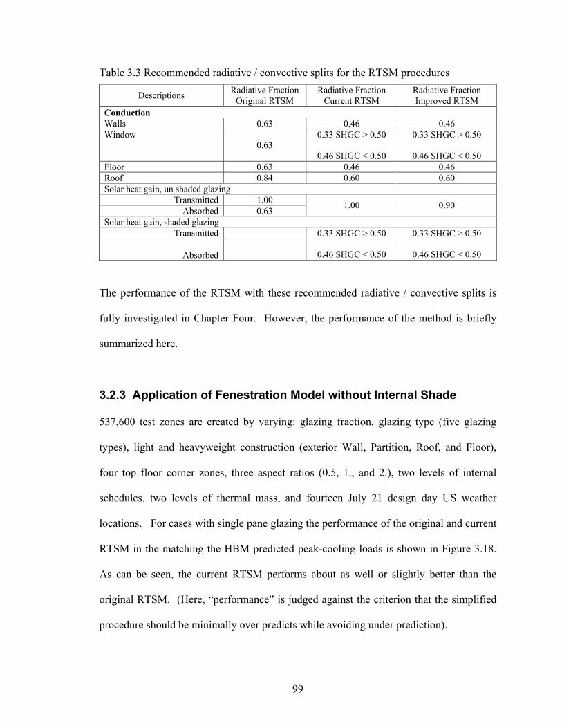
99
Table 3.3 Recommended radiative / convective splits for the RTSM procedures
Descriptions Radiative Fraction Original RTSM
Radiative Fraction Current RTSM
Radiative Fraction Improved RTSM
Conduction Walls 0.63 0.46 0.46 Window
0.63 0.33 SHGC > 0.50
0.46 SHGC < 0.50
0.33 SHGC > 0.50
0.46 SHGC < 0.50 Floor 0.63 0.46 0.46 Roof 0.84 0.60 0.60 Solar heat gain, un shaded glazing
Transmitted 1.00 Absorbed 0.63 1.00 0.90
Solar heat gain, shaded glazing Transmitted
Absorbed
0.33 SHGC > 0.50
0.46 SHGC < 0.50
0.33 SHGC > 0.50
0.46 SHGC < 0.50
The performance of the RTSM with these recommended radiative / convective splits is
fully investigated in Chapter Four. However, the performance of the method is briefly
summarized here.
3.2.3 Application of Fenestration Model without Internal Shade
537,600 test zones are created by varying: glazing fraction, glazing type (five glazing
types), light and heavyweight construction (exterior Wall, Partition, Roof, and Floor),
four top floor corner zones, three aspect ratios (0.5, 1., and 2.), two levels of internal
schedules, two levels of thermal mass, and fourteen July 21 design day US weather
locations. For cases with single pane glazing the performance of the original and current
RTSM in the matching the HBM predicted peak-cooling loads is shown in Figure 3.18.
As can be seen, the current RTSM performs about as well or slightly better than the
original RTSM. (Here, “performance” is judged against the criterion that the simplified
procedure should be minimally over predicts while avoiding under prediction).
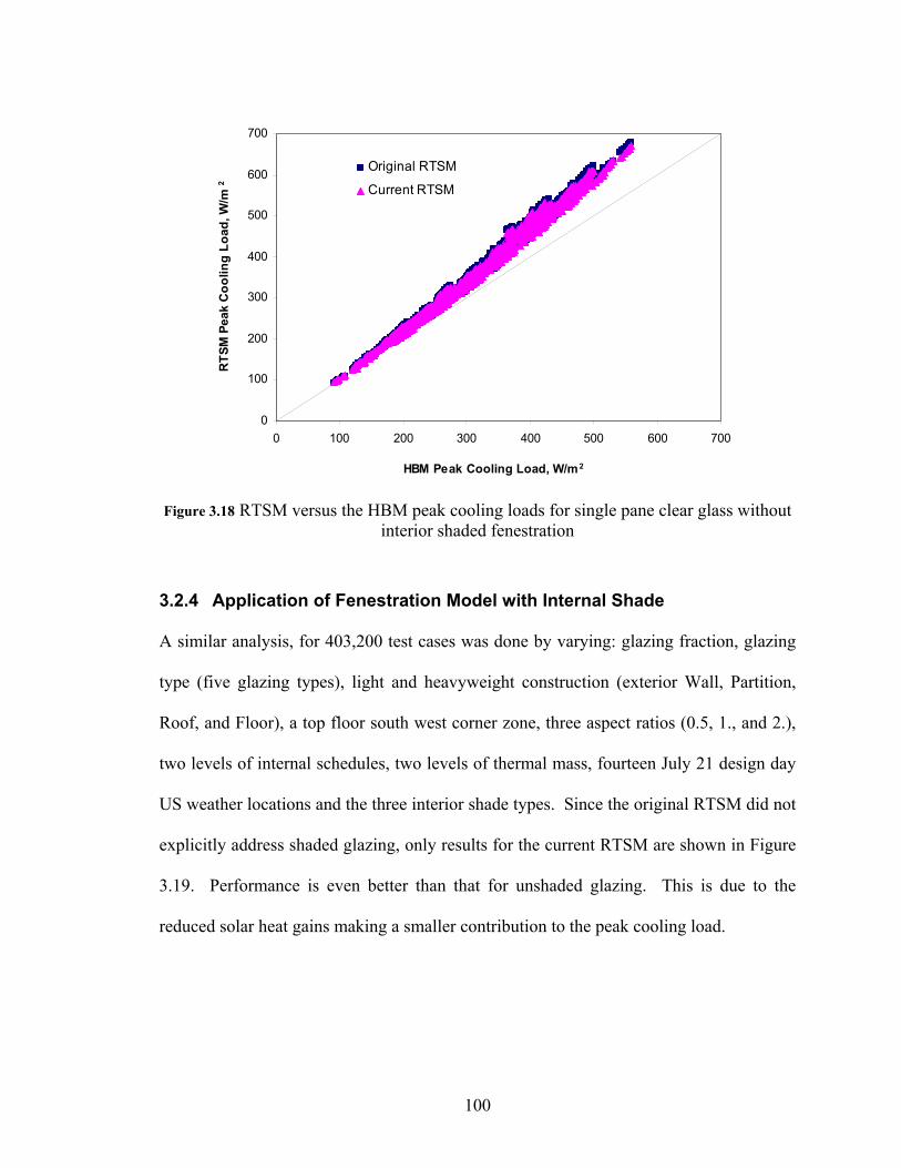
100
0
100
200
300
400
500
600
700
0 100 200 300 400 500 600 700
HBM Peak Cooling Load, W/m2
RTS
M P
eak
Coo
ling
Load
, W/m
2
Original RTSM
Current RTSM
Figure 3.18 RTSM versus the HBM peak cooling loads for single pane clear glass without
interior shaded fenestration
3.2.4 Application of Fenestration Model with Internal Shade
A similar analysis, for 403,200 test cases was done by varying: glazing fraction, glazing
type (five glazing types), light and heavyweight construction (exterior Wall, Partition,
Roof, and Floor), a top floor south west corner zone, three aspect ratios (0.5, 1., and 2.),
two levels of internal schedules, two levels of thermal mass, fourteen July 21 design day
US weather locations and the three interior shade types. Since the original RTSM did not
explicitly address shaded glazing, only results for the current RTSM are shown in Figure
3.19. Performance is even better than that for unshaded glazing. This is due to the
reduced solar heat gains making a smaller contribution to the peak cooling load.
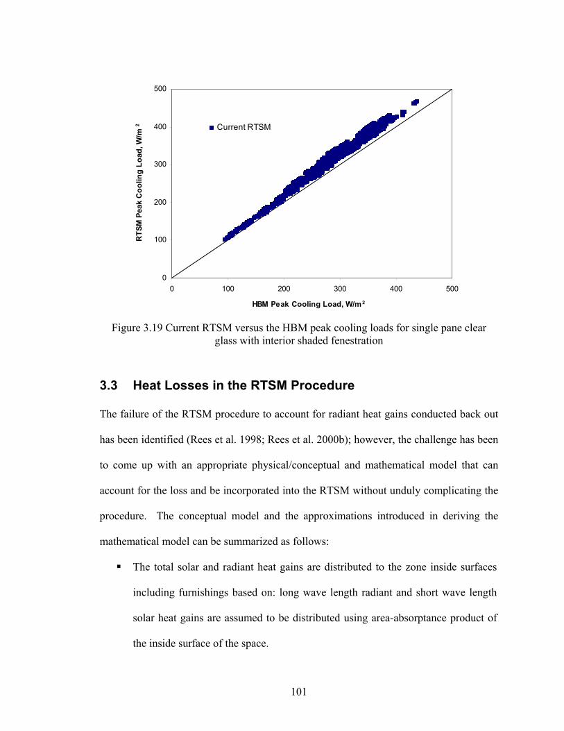
101
0
100
200
300
400
500
0 100 200 300 400 500
HBM Peak Cooling Load, W/m2
RTS
M P
eak
Coo
ling
Load
, W/m
2 Current RTSM
Figure 3.19 Current RTSM versus the HBM peak cooling loads for single pane clear
glass with interior shaded fenestration
3.3 Heat Losses in the RTSM Procedure
The failure of the RTSM procedure to account for radiant heat gains conducted back out
has been identified (Rees et al. 1998; Rees et al. 2000b); however, the challenge has been
to come up with an appropriate physical/conceptual and mathematical model that can
account for the loss and be incorporated into the RTSM without unduly complicating the
procedure. The conceptual model and the approximations introduced in deriving the
mathematical model can be summarized as follows:
The total solar and radiant heat gains are distributed to the zone inside surfaces
including furnishings based on: long wave length radiant and short wave length
solar heat gains are assumed to be distributed using area-absorptance product of
the inside surface of the space.
102
The procedure assumes the fenestration inside surfaces radiate to the room air.
This assumption decouples the long wavelength radiation exchange among the
surfaces in the zone and allows each surface to be treated separately.
Uses a fixed combined inside surface conductance. This assumption along with
previous approximations allows introducing the concept of inside sol-air
temperature concept.
The surface heat balance ignores the thermal mass of the fenestration; hence,
steady state analysis is valid.
Short-wave retransmission losses are ignored both in the HBM and RTSM. The
window is assumed opaque to long wavelength radiation.
These assumptions and approximations along with the conceptual model leads to the
formulation of an algorithm that accounts for radiant heat gain instantaneously conducted
through fenestrations using a dimensionless loss conductance.
3.3.1 Derivation of the Mathematical Algorithm
The procedure assumes steady state conditions, considering the thermal mass of the
fenestration to be negligible, and estimates how much of the radiant (solar and internal
heat gains) are conducted back out of the windows. Fenestration conduction heat gain
calculations in the original RTSM consider only the effects of the outdoor and indoor air
temperatures:
( )aocond TTUq −=''& (3.23)
103
Solar heat gain coefficients are mainly intended for rating of the fenestration and do not
take into account the fenestration interaction with the space heat gains and other inside
surfaces. In reality, the fenestration interaction with the space heat gain may lead to net
conduction heat gain into the space or conduction back out depending on the amount of
space heat gain, outdoor air temperature and fenestration conductance.
What is missing in the original RTSM procedure is a procedure that integrates the effect
of space solar and radiant internal heat gains and the outdoor air temperature into the
fenestration conduction analysis. Derivation of the adapted fenestration conduction
equation that combines these effects along with the assumptions introduced is described
next. The following assumptions were introduced to formulate the heat conduction
equation that account for the space heat gain loss:
The total solar and internal radiant heat gains are distributed to the zone inside
surfaces including furnishings based on: long wavelength radiant and short
wavelength solar heat gains are assumed to be distributed using area-absorptance
product of the inside surface of the space.
Uses combined inside surface conductance.
The surface heat balance ignores the thermal mass of the fenestration; hence,
steady state analysis is valid.
Short wave retransmission losses are ignored both in the HBM and RTSM. The
window is assumed opaque to long wavelength radiation.

104
The derivation of the radiant heat gain back loss equations is developed based on area-
absorptance product radiant heat gains distribution model as a generalized expression.
For this approach, long and short wavelength radiant heat gains and inside surface
absorptivities would have to be tracked separately. But the expression can be reduced
further to much simpler form with area-weighted distribution model. The parametric run
results presented in Section 3.3.3 are based on area-weighted distribution models.
Fenestration inside Surface Heat Balance
The thermal network representation of a fenestration with solar and internal heat gain
flux absorbed on the inside surface is shown in Figure 3.20.
Figure 3.20 Representation of fenestration inside surface heat balance
105
Using combined inside conductance and a prescribed the space radiant heat gain
distribution model, the instantaneous fenestration inside surface heat balance assuming a
steady state condition by ignoring the thermal mass is given by:
( ) ( ) 0", =+−+− asiaicbsiosi qTThTTU & (3.24)
Where,
Usi = the U value from outdoor air to the inside surface, W/m2⋅K
To = outdoor air temperature, °C
Ta = indoor air temperature, °C
hcb,i = inside surface combined conductance, W/m2⋅K
Tsi = the inside surface temperature, °C
"aq& = the space radiant heat gains distributed to the inside surface of the
fenestration, W/m2
Solving Eq. 3.24 for the inside surface temperature yields:
icbsi
aa
icbsi
icbo
icbsi
sisi hU
qThU
hT
hUUT
,
"
,
,
, ++
++
+=
& (3.25)
The Usi is related to the air-to-air U-value and the inside combined conductance by:
106
siicb UhU111
,
+= (3.26)
Starting from Eqn (3.26), the following simplifications can be derived for the coefficients
in Eqn 3.25.
icbicbsi
si
hU
hUU
,,
=+
(3.27)
siicbsi
icb
UU
hUh
=+ ,
, (3.28)
icbsiicbsi hUU
hU ,,
1=
+ (3.29)
Substituting Eqs. 3.27, 3.28, and 3.29 into Eq. 3.25 and simplifying yields:
"
,,a
icbsia
sio
icbsi q
hUUT
UUT
hUT &++= (3.30)
An inside sol-air temperature may be defined as an artificial air temperature that gives the
same heat gain/loss as the combined radiation and convection:
( ) ( )aSiicbSAio TThTTU −=− , (3.31)
Or
( )asiicb
oSAi TTU
hTT −−= , (3.32)
107
Substituting for the inside surface temperature (Eq. 3.30) into Eq. 3.32 yields:
−++−= aa
icbsia
sio
icb
icboSAi Tq
hUUT
UUT
hU
Uh
TT "
,,
, & (3.33)
Simplifying yields:
aicb
asi
asi
icbooSAi T
Uh
qU
TUh
TTT ,", 1+−−−= & (3.34)
",
111a
sia
siicbSAi q
UT
UUhT &−
−= (3.35)
"
,,
11a
sia
icbicbSAi q
UT
hhT &−
= (3.36)
"1a
siaSAi q
UTT &−= (3.37)
The conduction heat gain through the ith window (fenestration) that includes the effects of
radiant heat gains absorbed on the inside surface is then given by:
( )SAiocond TTUq −="& (3.38)
Substituting for the inside sol-air temperature TSAi and rearranging yields:
108
( )
+−= ""
asi
aocond qUUTTUq && (3.39)
And, rearranging Eqns. 3.26 gives:
icbsi hU
UU
,
1−= (3.40)
Substituting Eq. 3.40 into Eq 3.39 allows the elimination of Usi.
( ) 1 "
,
"a
icbaocond q
hUTTUq &&
−+−= (3.41)
( ) "
,
""a
icbaaocond q
hUqTTUq &&& −+−= (3.42)
The first two terms in Eq. 3.44 represent the conduction heat gain and the radiant heat
gain flux absorbed by the inside fenestration surface, respectively. The last term is the
amount of space radiant heat gain conducted back out through the fenestration. The
amount of space heat gain absorbed by the fenestration depends on the heat gain
distribution and surface properties. To simplify the procedure, the heat gain absorbed by
the fenestration inside surface needs to be expressed in terms of the space heat gain and
prescribed distribution function. Area-absorptance product weighted distribution can be
used to approximate the heat absorbed by surfaces. Using this distribution model the
space radiant heat gain absorbed by a surface is given by:
109
j
HGN
jjj
jja A
q
A
Aq
&&
=
∑=1
" α
α (3.43)
Where,
HGq& = the space solar and internal radiant heat gains, W
N = the number of surfaces of the zone
αj = the absorptance of the jth surface appropriate to short and long wavelength
heat gain type, (-)
Eq. 3.43 may reduce to simple area-fraction provided the inside absorptance of the
surfaces in the zone are the same. For a first order approximation of the space radiant
heat gain loss the area fraction should be sufficient. Substituting Eq. (3.43) into Eq.
(3.42) the expression for conduction heat gain/loss flux that combines the effect of the
space radiant heat gain is given by:
( )
1
,
1
",
j
HGN
jjj
jj
icbj
HGN
jjj
jjaojcond A
q
A
AhU
Aq
A
ATTUq
&&&
−
+−=
∑∑==
α
α
α
α (3.44)
( )
1
,
1
, HGN
jjj
jj
icbHGN
jjj
jjaojjcond q
A
AhUq
A
ATTUAq &&&
−
+−=
∑∑==
α
α
α
α (3.45)
110
Further simplification of the overall heat conduction equation that takes into account the
space radiant heat gain may lead to four different approaches for implementing in the
RTSM cooling load calculation procedure:
An improved heat conduction equation which would replace the existing
equations for fenestration heat gain due to temperature difference between the
inside and outside can be developed. Instead of using the inside air temperature,
an expression for inside sol-air temperature can be developed and utilized.
Although this follows the physics in a way analogous to the exterior sol-air
temperature, it seems likely to be confusing to users of the method. (Approach I)
A dimensionless loss coefficient, *u , can be developed and applied to all of the
radiant heat gains. (Approach II)
A correction to the first term of the radiant time factor series can be made.
(Approach III)
A modified heat conduction equation that accounts for the heat gain loss can be
formulated. (Approach IV).
The derivation for all four approaches utilizes an interior sol-air temperature as described
below. However, for the II, III and IV approach, interior sol-air temperature is
eliminated.
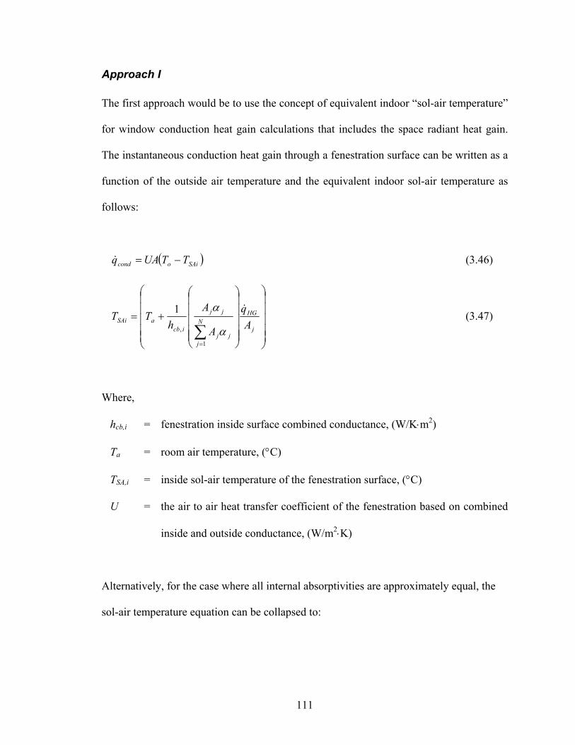
111
Approach I
The first approach would be to use the concept of equivalent indoor “sol-air temperature”
for window conduction heat gain calculations that includes the space radiant heat gain.
The instantaneous conduction heat gain through a fenestration surface can be written as a
function of the outside air temperature and the equivalent indoor sol-air temperature as
follows:
( ) SAiocond TTUAq −=& (3.46)
+=
∑=
j
HGN
jjj
jj
icbaSAi A
q
A
Ah
TT&
1
,
1
α
α (3.47)
Where,
hcb,i = fenestration inside surface combined conductance, (W/K⋅m2)
Ta = room air temperature, (°C)
TSA,i = inside sol-air temperature of the fenestration surface, (°C)
U = the air to air heat transfer coefficient of the fenestration based on combined
inside and outside conductance, (W/m2⋅K)
Alternatively, for the case where all internal absorptivities are approximately equal, the
sol-air temperature equation can be collapsed to:
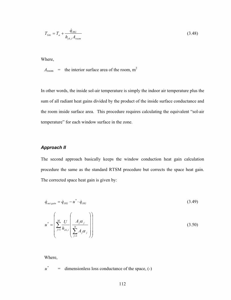
112
roomicb
HGaSAi Ah
qTT
,
&+= (3.48)
Where,
Aroom = the interior surface area of the room, m2
In other words, the inside sol-air temperature is simply the indoor air temperature plus the
sum of all radiant heat gains divided by the product of the inside surface conductance and
the room inside surface area. This procedure requires calculating the equivalent “sol-air
temperature” for each window surface in the zone.
Approach II
The second approach basically keeps the window conduction heat gain calculation
procedure the same as the standard RTSM procedure but corrects the space heat gain.
The corrected space heat gain is given by:
HGHGgainnet quqq &&& * ⋅−= (3.49)
= ∑∑=
=
M
jN
jjj
jj
icb A
AhUu
1
1
,
*
α
α (3.50)
Where,
*u = dimensionless loss conductance of the space, (-)
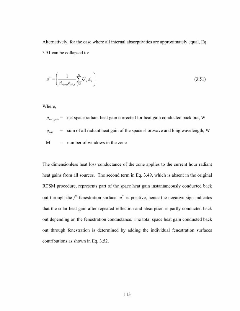
113
Alternatively, for the case where all internal absorptivities are approximately equal, Eq.
3.51 can be collapsed to:
= ∑
=
M
jjj
icbroom
AUhA
u1,
* 1 (3.51)
Where,
gainnetq ,& = net space radiant heat gain corrected for heat gain conducted back out, W
HGq& = sum of all radiant heat gain of the space shortwave and long wavelength, W
M = number of windows in the zone
The dimensionless heat loss conductance of the zone applies to the current hour radiant
heat gains from all sources. The second term in Eq. 3.49, which is absent in the original
RTSM procedure, represents part of the space heat gain instantaneously conducted back
out through the jth fenestration surface. *u is positive, hence the negative sign indicates
that the solar heat gain after repeated reflection and absorption is partly conducted back
out depending on the fenestration conductance. The total space heat gain conducted back
out through fenestration is determined by adding the individual fenestration surfaces
contributions as shown in Eq. 3.52.
114
HG
M
jN
jjj
jj
icbLoss q
A
AhUq && ⋅
= ∑
∑=
=
1
1
, α
α (3.52)
Where,
M = the number of fenestrations in the zone, (-)
The assumptions introduced to derive Eq. 3.51 are in many ways similar to the
simplification used in the derivation of the RTSM. It is evident from Eq. 3.51 that the
space heat gain that could be conducted back out depends on the amount of solar heat
gain into the space, the dimensionless conductance of the space, and the space heat gain
distribution. In reality solar and internal radiant heat gain could be conducted back out
through opaque exterior constructions; however, the amount is smaller compared to that
of the fenestrations; hence, can be ignored.
Approach III
Examining the form of the correction factor in Eq. 3.45 shows that it operates on the
current hour of the solar and internal radiant heat gains, as does the first term of the
radiant time factor series. The correction factor can be readily integrated to the radiant
time factors and the original RTSM calculation procedure is retained. Therefore,
approach III can be introduced as a correction to the first term of RTF. The beauty of the
third approach is that it can be implemented simply by subtracting the dimensionless heat
loss conductance from the first term of the radiant time factors without any change to the
115
original RTSM procedure. The corrected radiant time factors, solar and non-solar, are
given by:
( )*0,0, urr ss −= (3.53)
( )*0,0, urr nsns −= (3.54)
Therefore, approach III simply reduces to correcting the instantaneous term (the first
term) of the radiant time factors. *u is a positive dimensionless conductance determined
from construction fabrics, area and absorptance of the surfaces. The effect of this
approach is then it will correct all radiant heat gains that are operated by radiant time
factors. Therefore, approach III automatically accounts for the conduction loss from the
radiant fraction of conduction heat gains through the fenestrations, which cannot be done
without extra effort in approaches II and I.
Approach IV
The conduction heat gain through fenestrations that accounts for the effect of the space
radiant heat gain can be formulated using the Eq 3.48 for sol-air temperature and Eq. 3.46
and is given by:
,
−−=
roomicb
HGaocond Ah
qTTUAq
&& (3.55)
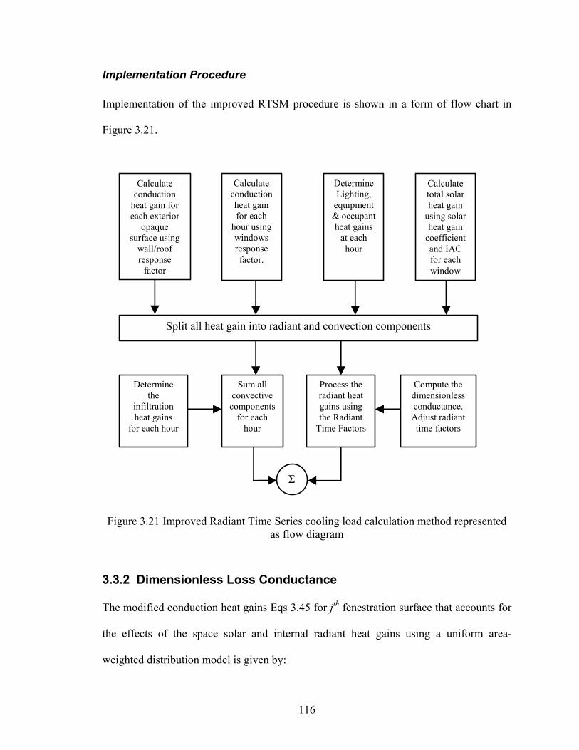
116
Implementation Procedure
Implementation of the improved RTSM procedure is shown in a form of flow chart in
Figure 3.21.
DetermineLighting,
equipment& occupant heat gains
at each hour
Calculate conduction heat gain for each
hour using windows response factor.
Calculate conduction
heat gain for each exterior
opaque surface using
wall/roof response
factor
Calculate total solar heat gain
using solar heat gain
coefficient and IAC for each window
Split all heat gain into radiant and convection components
Determine the
infiltration heat gains
for each hour
Sum all convective
components for each
hour
Process the radiant heat gains using the Radiant
Time Factors
Σ
Compute the dimensionless conductance. Adjust radiant time factors
Figure 3.21 Improved Radiant Time Series cooling load calculation method represented
as flow diagram
3.3.2 Dimensionless Loss Conductance
The modified conduction heat gains Eqs 3.45 for jth fenestration surface that accounts for
the effects of the space solar and internal radiant heat gains using a uniform area-
weighted distribution model is given by:
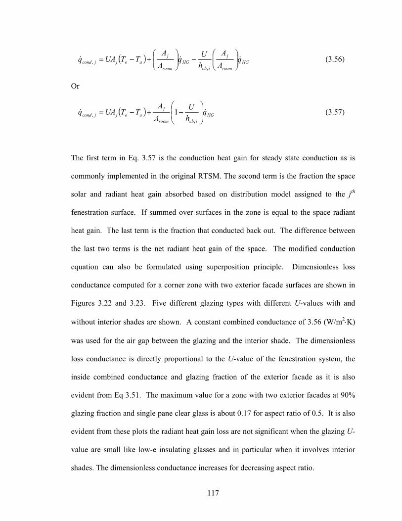
117
( ) ,
, HGroom
j
icbHG
room
jaojjcond q
AA
hUq
AA
TTUAq &&&
−
+−= (3.56)
Or
( ) 1,
, HGicbroom
jaojjcond q
hU
AA
TTUAq &&
−+−= (3.57)
The first term in Eq. 3.57 is the conduction heat gain for steady state conduction as is
commonly implemented in the original RTSM. The second term is the fraction the space
solar and radiant heat gain absorbed based on distribution model assigned to the jth
fenestration surface. If summed over surfaces in the zone is equal to the space radiant
heat gain. The last term is the fraction that conducted back out. The difference between
the last two terms is the net radiant heat gain of the space. The modified conduction
equation can also be formulated using superposition principle. Dimensionless loss
conductance computed for a corner zone with two exterior facade surfaces are shown in
Figures 3.22 and 3.23. Five different glazing types with different U-values with and
without interior shades are shown. A constant combined conductance of 3.56 (W/m2⋅K)
was used for the air gap between the glazing and the interior shade. The dimensionless
loss conductance is directly proportional to the U-value of the fenestration system, the
inside combined conductance and glazing fraction of the exterior facade as it is also
evident from Eq 3.51. The maximum value for a zone with two exterior facades at 90%
glazing fraction and single pane clear glass is about 0.17 for aspect ratio of 0.5. It is also
evident from these plots the radiant heat gain loss are not significant when the glazing U-
value are small like low-e insulating glasses and in particular when it involves interior
shades. The dimensionless conductance increases for decreasing aspect ratio.
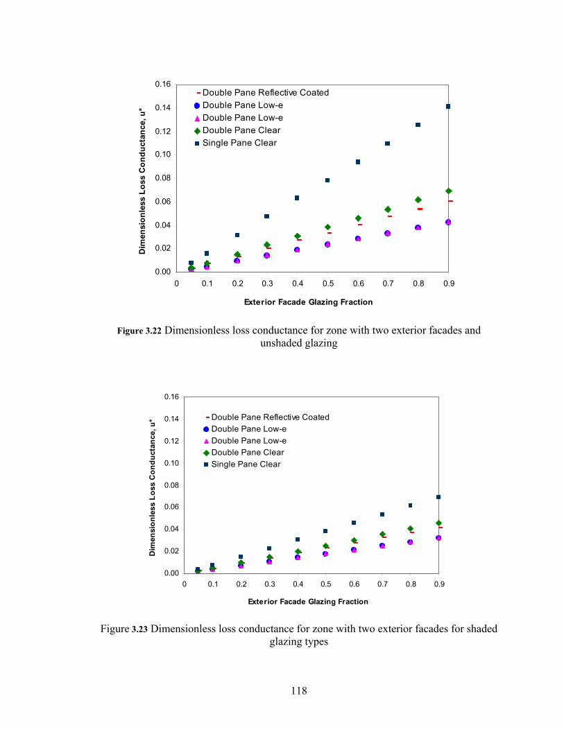
118
0.00
0.02
0.04
0.06
0.08
0.10
0.12
0.14
0.16
0 0.1 0.2 0.3 0.4 0.5 0.6 0.7 0.8 0.9
Exterior Facade Glazing Fraction
Dim
ensi
onle
ss L
oss
Con
duct
ance
, u*
Double Pane Reflective Coated Double Pane Low-eDouble Pane Low-eDouble Pane ClearSingle Pane Clear
Figure 3.22 Dimensionless loss conductance for zone with two exterior facades and
unshaded glazing
0.00
0.02
0.04
0.06
0.08
0.10
0.12
0.14
0.16
0 0.1 0.2 0.3 0.4 0.5 0.6 0.7 0.8 0.9
Exterior Facade Glazing Fraction
Dim
ensi
onle
ss L
oss
Con
duct
ance
, u* Double Pane Reflective Coated
Double Pane Low-eDouble Pane Low-eDouble Pane ClearSingle Pane Clear
Figure 3.23 Dimensionless loss conductance for zone with two exterior facades for shaded
glazing types
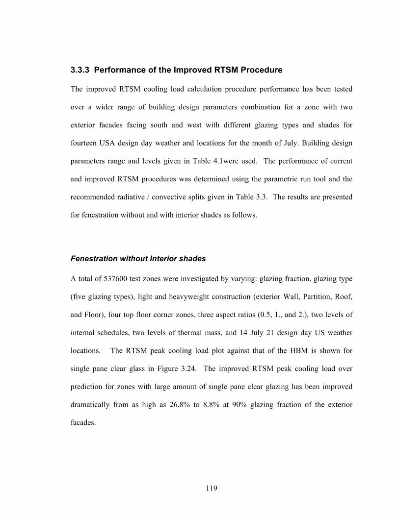
119
3.3.3 Performance of the Improved RTSM Procedure
The improved RTSM cooling load calculation procedure performance has been tested
over a wider range of building design parameters combination for a zone with two
exterior facades facing south and west with different glazing types and shades for
fourteen USA design day weather and locations for the month of July. Building design
parameters range and levels given in Table 4.1were used. The performance of current
and improved RTSM procedures was determined using the parametric run tool and the
recommended radiative / convective splits given in Table 3.3. The results are presented
for fenestration without and with interior shades as follows.
Fenestration without Interior shades
A total of 537600 test zones were investigated by varying: glazing fraction, glazing type
(five glazing types), light and heavyweight construction (exterior Wall, Partition, Roof,
and Floor), four top floor corner zones, three aspect ratios (0.5, 1., and 2.), two levels of
internal schedules, two levels of thermal mass, and 14 July 21 design day US weather
locations. The RTSM peak cooling load plot against that of the HBM is shown for
single pane clear glass in Figure 3.24. The improved RTSM peak cooling load over
prediction for zones with large amount of single pane clear glazing has been improved
dramatically from as high as 26.8% to 8.8% at 90% glazing fraction of the exterior
facades.
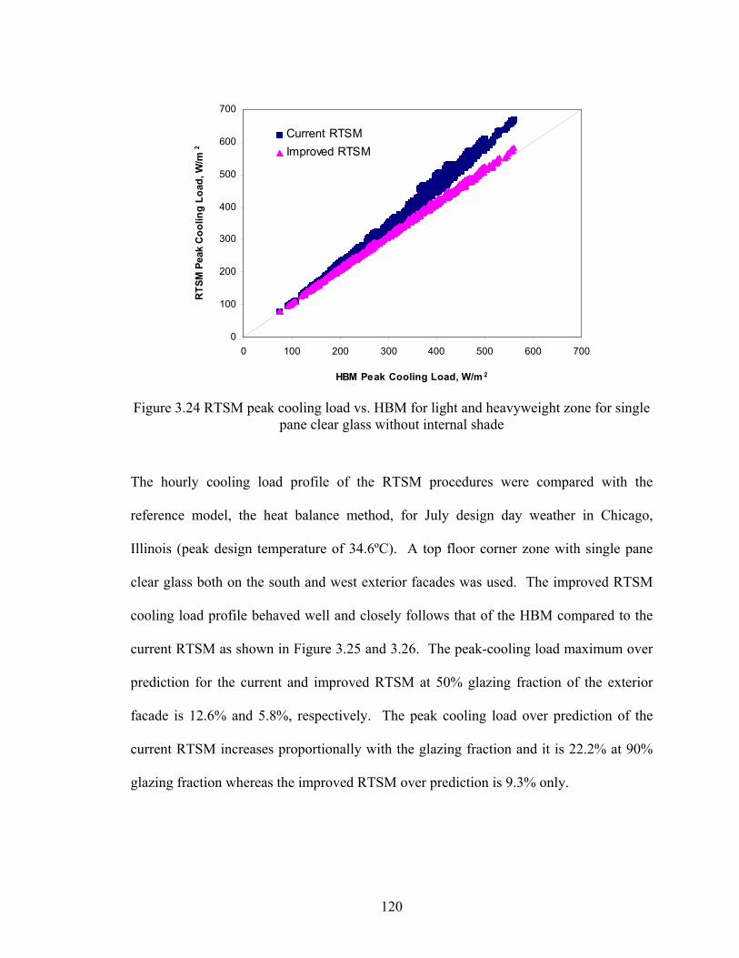
120
0
100
200
300
400
500
600
700
0 100 200 300 400 500 600 700
HBM Peak Cooling Load, W/m 2
RTS
M P
eak
Coo
ling
Load
, W/m
2
Current RTSMImproved RTSM
Figure 3.24 RTSM peak cooling load vs. HBM for light and heavyweight zone for single
pane clear glass without internal shade
The hourly cooling load profile of the RTSM procedures were compared with the
reference model, the heat balance method, for July design day weather in Chicago,
Illinois (peak design temperature of 34.6ºC). A top floor corner zone with single pane
clear glass both on the south and west exterior facades was used. The improved RTSM
cooling load profile behaved well and closely follows that of the HBM compared to the
current RTSM as shown in Figure 3.25 and 3.26. The peak-cooling load maximum over
prediction for the current and improved RTSM at 50% glazing fraction of the exterior
facade is 12.6% and 5.8%, respectively. The peak cooling load over prediction of the
current RTSM increases proportionally with the glazing fraction and it is 22.2% at 90%
glazing fraction whereas the improved RTSM over prediction is 9.3% only.
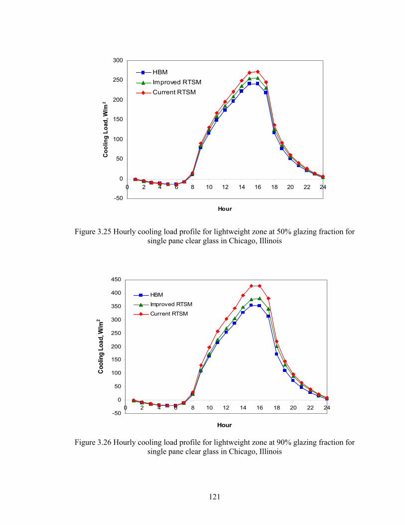
121
-50
0
50
100
150
200
250
300
0 2 4 6 8 10 12 14 16 18 20 22 24
Hour
Cool
ing
Load
, W/m
2
HBMImproved RTSMCurrent RTSM
Figure 3.25 Hourly cooling load profile for lightweight zone at 50% glazing fraction for
single pane clear glass in Chicago, Illinois
-50
0
50
100
150
200
250
300
350
400
450
0 2 4 6 8 10 12 14 16 18 20 22 24
Hour
Cool
ing
Load
, W/m
2
HBM
Improved RTSM
Current RTSM
Figure 3.26 Hourly cooling load profile for lightweight zone at 90% glazing fraction for
single pane clear glass in Chicago, Illinois
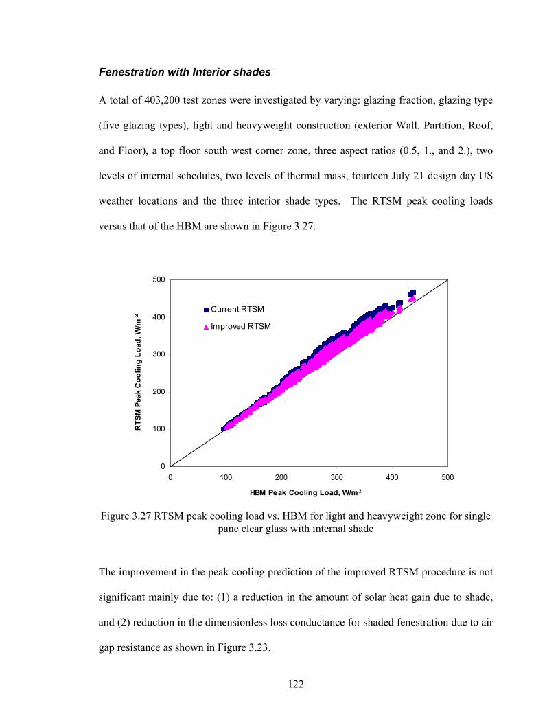
122
Fenestration with Interior shades
A total of 403,200 test zones were investigated by varying: glazing fraction, glazing type
(five glazing types), light and heavyweight construction (exterior Wall, Partition, Roof,
and Floor), a top floor south west corner zone, three aspect ratios (0.5, 1., and 2.), two
levels of internal schedules, two levels of thermal mass, fourteen July 21 design day US
weather locations and the three interior shade types. The RTSM peak cooling loads
versus that of the HBM are shown in Figure 3.27.
0
100
200
300
400
500
0 100 200 300 400 500
HBM Peak Cooling Load, W/m2
RTS
M P
eak
Coo
ling
Load
, W/m
2
Current RTSM
Improved RTSM
Figure 3.27 RTSM peak cooling load vs. HBM for light and heavyweight zone for single
pane clear glass with internal shade
The improvement in the peak cooling prediction of the improved RTSM procedure is not
significant mainly due to: (1) a reduction in the amount of solar heat gain due to shade,
and (2) reduction in the dimensionless loss conductance for shaded fenestration due to air
gap resistance as shown in Figure 3.23.
123
The RTSM peak cooling load over predictions in design weather location of Atlanta,
Georgia for lightweight construction zone with dark roller interior shaded and single pane
clear glass is well below 6% for current procedure and well below 3% for the improved
procedures. However, the peak cooling load over prediction is relatively higher for
heavyweight construction zones and can be as high as 12% and 9% for current and
improved RTSM, respectively. The main reason for marked difference in performance of
the RTSM for light and heavy weight construction zones is the use of fixed radiative
fraction for all construction types.
Heavyweight construction zone with interior shaded fenestration surfaces require higher
radiative fractions due to the lower mean radiant temperatures they see compared to
lightweight construction zones. Based on higher radiative fractions for heavyweight
construction zones the RTSM peak cooling load predictions would have been less. The
higher sensitivities of the RTSM performance to construction fabrics for fenestration with
shades is that most of the solar heat gains is transmitted into the space via radiation
exchange after being absorbed by the shade. Moreover, the radiant fraction is dependent
on the mean radiant temperatures of surfaces viewed by the fenestration, which also
depends on the zone construction fabrics. As the results the radiative fraction of solar
and conduction heat gains of fenestrations with interior shades shows more sensitivity
compared to fenestration without interior shade, for which the solar heat gain is mainly
transmitted component.
124
The RTSM peak cooling over prediction shows good match with the HBM for larger
aspect ratios. The higher over prediction at lower aspect ratio in particular to
heavyweight construction zones is due to large amount of solar heat gain per unit floor
area and the sensitivity of the radiative / convective split to construction fabrics.
However, the improved RTSM procedure peak cooling load shows less sensitivity to
aspect ratio compared to the current RTSM procedure.
3.3.4 Heat Losses in the TFM Procedure
Spitler and Fisher (1999) introduced a relationship between the RTSM radiant time
factors and the weighting factors of the TFM using the steady periodic nature of the
design day cooling load calculation. On this basis, it seems likely that a similar heat
losses correction could be derived for the TFM. Indeed, this is the case. The derivation
is given in this section.
The current hour cooling loads are related to the hourly present and past heat gains using
the heat gain weighting factor transfer function method formulation described by Kerrisk
(1981) and is given by:
∑∑=
−=
− −=2
1
2
0 kkk
jjj QwqQ δθδθθ ν (3.58)
Calculation of steady periodic radiant time series coefficient matrix is defined in terms of
the zone weighting factors coefficient matrices and is given by:
125
VWR 1−= (3.59)
Where W is the cooling load weighting factor coefficient matrix, V is the heat gain
weighting factor coefficients matrix, and R is the radiant time factors coefficient matrix.
The dimensionless loss conductance is introduced to account for the space radiant heat
gain conducted back out and acts on the current hour of the radiant time factors. For a
steady periodic design day load calculation the corrected radiant time factors coefficient
matrix is given by:
IRR *u−= (3.60)
Where R is the corrected radiant time factor coefficients matrix and I is the identity
matrix. Taking the steady periodic nature of the design day load calculation the improved
RTSM procedure that accounts for the radiant heat back loss can be related to the transfer
function weighting factors using the relationship described by Spitler and Fisher (1999)
and it is given by:
[ ] qq VWIR 1−=+ *u (3.61)
Where q is a column vector contains the 24 hourly values of the radiant heat gains.
Dropping the heat gains vectors form both sides of the equation and multiplying both
sides of the equation by W and simplifying yields:
126
[ ] VIWRW =+ *u (3.62)
RWV = (3.63)
Where V is the corrected the heat gain weighting factors coefficient matrix.
Substituting Eq. 3.63 into Eq. 3.62 and rearing yields:
WVV *u+= (3.64)
WVV *u−= (3.65)
Eq. 3.65 relates the corrected heat gain weighting factor coefficient matrix to the
adiabatic (normalized) heat gain TFM weighting factors and cooling load TFM weighting
factors coefficient matrix using the dimensionless loss conductance.
3.3.5 Conclusion and Recommendations
It has been a problem to formulate a procedure that accounts for the radiant heat gain loss
yet maintains the simplicity of the RTSM procedure. A methodology or an algorithm
that accounts for radiant heat gain back loss and mitigates the RTSM peak-cooling load
over predictions has been developed. This algorithm introduces a dimensionless loss
conductance of a zone that depends on the fenestration U-value, inside combined
conductance, fenestration area and the inside surface areas. This algorithm has been
tested over wide range building design parameters combination forming 403,200 test
cases for shaded fenestration and 537,600 test cases for unshaded one. The modification
and implementation of the algorithm maintains the simplicity of the original RTSM
127
procedure and can be adopted by simply correcting the first terms of the adiabatic radiant
time factors. The following conclusions can be drawn from the finding of the parametric
run investigation of the RTSM procedure:
The dimensionless loss conductance that accounts for heat loss of a space has
been introduced and can be computed readily from building design parameters –
the fenestration U-value and area, inside combined conductance and zone inside
surface area. The heat losses are not significant when the glazing U-value is
small like in insulating glasses and in particular when it involves interior shades.
In general the improved RTSM reduces the peak-cooling load over prediction
trend of the RTSM procedure dramatically. The peak cooling load over
prediction can be reduced fewer than 10% for zones with single pane clear glasses
and having two exterior facades for most design weather conditions. The over
prediction of peak cooling load is much lower in the glazing fraction is less than
70%. In general peak cooling load over predictions of the RTSM procedure for
light weight construction zones is much lower than heavyweight construction
zones without interior shaded fenestrations. The improved RTSM peak cooling
load over prediction for lightweight construction zones with unshaded
fenestration is less 6%.
Two range solar heat gain radiative / convective splits were recommended that
depends on the glazing type for fenestration with interior shades. The improved
RTSM procedure works better if several ranges of radiative / convective splits
that depend on glazing type for zones without interior shaded fenestration. The
radiative / convective split used for solar heat gain in the RTSM procedure
128
showed strong sensitivity to zone construction fabric for fenestration system with
interior shades. Though a fixed value use of radiative fraction for all construction
fabrics showed conservative estimate of the RTSM peak cooling load, the over
prediction trend can further be reduced by using radiative fraction dependent on
the zone construction fabrics as well. With recommended radiative / convective
split given in Table 3.3 the maximum over prediction of the improved RTSM may
reach as high as 11% for heavyweight construction zones. The over prediction of
the RTSM can be further reduced for fenestration system without shades by using
a radiative / convective split dependent on the glazing type and construction
fabrics.
Further investigation is required to determine the radiative / convective splits
dependency on other types of interior shades like drapery fabrics with wide
characteristics of optical properties.
3.4 Summary and Conclusions The series of improvements to the Radiant Time Series Method investigated developed in
this chapter are comprised of improvements of the method, its sub-models, or supporting
data, or ease of implementation in various computing environments. These
improvements are summarized as follows:
A one-dimensional finite volume procedure with fully implicit solution scheme has
been developed for PRF generation. The PRFs are generated by exciting multi-
layered wall with unit height triangular base temperature pulse. The procedure uses
uniform gridding for each layer with zero thickness boundary nodes for effective
boundary condition imposition. Moreover, higher order expression is used for
129
response flux calculation. The algorithm has been implemented in FORTRAN 90,
VBA and SCILAB. The implementations in these programming platforms required
500, 450 and 150 lines of code, respectively, compared to 2000 lines of FORTRAN
90 for computation of CTF with the State Space method and conversion to PRF.
The finite volume procedure has been validated against PRF determined by
converting CTF generated using the State Space Method as discussed in Section
3.1.3. The validation was done comparing the peak heat gains computed using these
two PRF for typical design day sol-air temperatures and 82 ASHRAE walls and roofs
(ASHRAE, 1997). The difference between the peak heat gains is in the range -0.7%
to 2.2% and average error is -0.03%. The RMSE of the peak heat gain is 0.02 W/m2.
This is sufficient accuracy for cooling load calculation, as conduction heat gain is
small fraction of cooling loads.
The RTF generation procedure, which was originally developed using a full-blown
heat balance procedure, has been reformulated in a compact form is the “reduced heat
balance method” by eliminating unneeded features of the HBM. Due to the compact
nature of the algorithm it can take advantage of computing environments with built-in
libraries of matrix algebra. This algorithm has been successfully implemented in
VBA and SCILAB using 450 and 150 lines of codes, respectively. The procedure has
been validated against a full-blown heat balance procedure in Section 3.1.1. For six
test zones, the RMSE of the reduced heat balance procedure RTF compared to the full
heat balance method was within 0.00007 to 0.00037. This error margin is within the
convergence limits of the full-blown heat balance procedure. The reduced heat
balance procedure has been further simplified to use constant radiation coefficients
130
and this results in reducing the computation time by half compared to the variable
radiation coefficient implementation. With these simplifications the hourly cooling
load errors in a spreadsheet RTSM implementation for three test zones is within 0.02
Btu/hr⋅ft2. The hourly cooling load plots for constant and variable radiation
coefficient are shown in Appendix C.
An improved fenestration model, compatible with recent developments in fenestration
data, has been adapted to the RTSM procedure. A new set of radiative / convective
splits for fenestration conduction and solar heat gains have been established and are
given in Table 3.3. The RTSM fenestration model and the radiative / convective
splits fenestration model facilitates the use of manufactures’ data and avoids the need
for splitting solar heat gain into transmitted and absorbed components.
An algorithm for accounting heat losses by conduction through highly conductive
mass less surfaces such as fenestration has been developed. The algorithm uses a
dimensionless loss conductance that can be calculated from zone surface geometry,
fenestration U-value and combined inside surface conductance. The dimensionless
loss conductance operates on the first term of the radiant time factors and hence
maintains the simplicity of the RTSM procedure desired. The approximate correction
introduced reduced peak cooling load over predictions of the RTSM procedure
significantly for all problem zones. For a parametric study of 403,200 zones with
unshaded fenestration the maximum RTSM peak cooling load overprediction is
reduced from 26.8% to 8.8%.
131
CHAPTER IV
4. Parametric Study of the RTSM Procedure
This chapter deals with a parametric investigation conducted to develop quantitative
design guidance on the performance of the Radiant Time Series Method (RTSM). First,
the range of parameters investigated are described; second, the methodology employed in
the parametric investigation is explained and load calculation programs / software
utilized for the investigation are discussed; and, third the results and recommendations
are given.
Although the RTSM has been adopted by ASHRAE as published cooling load calculation
design procedure there is no information available regarding the likely overprediction of
the peak-cooling load by the RTSM procedure in the form of design guidance for
practicing engineers. It is difficult or impossible for a designer to judge the likely
overprediction of the RTSM in the absence of such quantitative design guidance. This
parametric study is intended to quantitatively investigate the effect of design parameters
that the influence the maximum overprediction error of the RTSM and lead to
quantitative design guidance. This work will make use of extended version of the
parametric run generation tool used in ASHRAE RP-942 but originally developed by
Strand as cited by Spitler and Rees (1998).
132
However, this work has a different goal - providing quantitative design guidance. In
addition, improvements to the fenestration model have been incorporated in both HBM
and RTSM procedures. The fenestration model is capable of modeling interior shades.
The HBM fenestration model is uses Klems (2002) algorithm given in appendix-A. The
RTSM fenestration model uses solar heat gain coefficient (SHGC), interior attenuation
coefficient (IAC) and radiative / convective split as described in Section 5.2. Compared
to the previous study (Rees et al. 1998; Spitler and Rees 1998) a much larger number of
parametric values and zones have been utilized.
4.1 Parametric Run Generation
This work utilized a revised version of the parametric run generation tool originally
developed by Strand as cited by Spitler and Rees (1998). The parametric run generator as
shown in Figure 4.1 reads in the input values for each parametric and levels and creates
input file each case. Three different “types” of parametric studies can be performed: a
“fully populated set”, a “sparsely populated set” and “min-max set” (Spitler and Rees
1998). The parametric run generator then creates a complete set of files for the specified
combinations of design parameters and the batch file required for running those
combinations. The individual zone input data is created by combining small text files
and, where necessary, computing dimensions and writing them into an input file.
Previously, the parametric run generator was limited to ten design days. It has been
updated to use up to 100 design different design days representing different locations and
months. This was needed to allow comparison for a range of months, as many zones do
not peak in summer. In this investigation, fourteen USA locations, each with seven
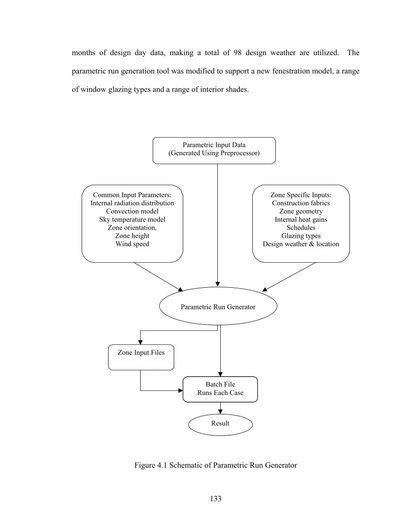
133
months of design day data, making a total of 98 design weather are utilized. The
parametric run generation tool was modified to support a new fenestration model, a range
of window glazing types and a range of interior shades.
Parametric Run Generator
Common Input Parameters: Internal radiation distribution
Convection model Sky temperature model
Zone orientation, Zone height Wind speed
Parametric Input Data (Generated Using Preprocessor)
Zone Specific Inputs: Construction fabrics
Zone geometry Internal heat gains
Schedules Glazing types
Design weather & location
Zone Input Files
Batch File Runs Each Case
Result
Figure 4.1 Schematic of Parametric Run Generator

134
4.2 Test Zone Parameters
This section discusses the range of zone parameters investigated in the parametric study.
The levels of the nineteen parameters summarized in Table 4.1 control the zone
construction, geometry, internal heat gains, and weather conditions. The levels reflect
typical values expected in practice. The numbering scheme has been adapted from
Spitler and Rees (1998), but not all of their levels are used. For example exterior wall
have levels, 1 and 6, levels 2-5 from Spitler and Rees (1998) are not used. Further
discussion of the changes in the parameter levels is given in the following sections.
Table 4.1 Test Parameter range and levels No Parameter No. of
Levels Parameter Levels
1 Room size 1 A: (6m east-west axis dimension)
2 Room level 2 m, t (middle & top floor zone)
3 Zone Number1 9 1 – 9 (all zone orientations)
4 % Glazing2 10 5%, 10%, 20%, 30%, …, 90%
5 People 3 5, 10 and 30 W per 100m2 (5, 10 and 30 per 1076 ft2)
6 Lighting 3 10, 20, and 30 W/m2 (3.17, 6.34 and 9.51 Btu/h ft2)
7 Equipment 1 30 W/m2 ( 9.51 Btu/h ft2)
8 Infiltration 1 0.5 Air change per hour (ACH)
9 Exterior Wall3 2
Type 1: light 32.0 kJ/m2⋅K (1.6 Btu/ft2 oF) Type 2: light 137.1 kJ/m2⋅K (6.7 Btu/ft2 oF) Type 3: light 316.6 kJ/m2⋅K (15.5 Btu/ft2 oF) Type 4: light 362.7 kJ/m2⋅K (17.7 Btu/ft2 oF) Type 5: light 520.7 kJ/m2⋅K (25.5 Btu/ft2 oF) Type 6: heavy 550.9 kJ/m2⋅K (26.9 Btu/ft2 oF)
10 Partition 2 Type 1: light 24.9 kJ/m2⋅K (1.2 Btu/ft2 oF) Type 2: heavy 208.9 kJ/m2⋅K (10.2 Btu/ft2 oF)
11 Roof 2 Type 1: light 34.4 kJ/m2⋅K (1.7 Btu/ft2 oF) Type 2: heavy 350.2 kJ/m2⋅K (17.1 Btu/ft2 oF)
12 Floor 2 Type 1: light 78.0 kJ/m2⋅K (3.8 Btu/ft2 oF) Type 4: heavy 540.7 kJ/m2⋅K (26.5 Btu/ft2 oF)
13 Ceiling 2 Type 1: light 78.0 kJ/m2⋅K (3.8 Btu/ft2 oF) Type 4: heavy 540.7 kJ/m2⋅K (26.5 Btu/ft2 oF)
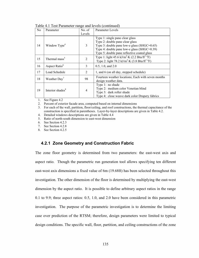
135
Table 4.1 Test Parameter range and levels (continued) No Parameter No. of
Levels Parameter Levels
14 Window Type4 3
Type 1: single pane clear glass Type 2: double pane clear glass Type 3: double pane low-e glass (SHGC=0.65) Type 4: double pane low-e glass (SHGC=0.39) Type 5: double pane reflective coated glass
15 Thermal mass5 2 Type 1: light 45.6 kJ/m2⋅K (2.2 Btu/ft2 oF) Type 2: light 78.2 kJ/m2⋅K (3.8 Btu/ft2 oF)
16 Aspect Ratio6 3 0.5, 1.0, and 2.0
17 Load Schedule 2 1, and 6 (on all day, stepped schedule)
18 Weather Day7 98 Fourteen weather locations; Each with seven months design weather data.
19 Interior shades8 4
Type 1: no shade Type 2: medium color Venetian blind Type 3: dark roller shade Type 4: close weave dark color Drapery fabrics
1. See Figure 4.2 2. Percent of exterior facade area, computed based on internal dimensions 3. For each of the wall, partition, floor/ceiling, and roof constructions, the thermal capacitance of the
construction is specified in parentheses. Layer-by-layer descriptions are given in Table 4.2. 4. Detailed windows descriptions are given in Table 4.4 5. Ratio of north-south dimension to east-west dimension 6. See Section 4.2.3 7. See Section 4.2.8 8. See Section 4.2.5
4.2.1 Zone Geometry and Construction Fabric
The zone floor geometry is determined from two parameters: the east-west axis and
aspect ratio. Though the parametric run generation tool allows specifying ten different
east-west axis dimensions a fixed value of 6m (19.68ft) has been selected throughout this
investigation. The other dimension of the floor is determined by multiplying the east-west
dimension by the aspect ratio. It is possible to define arbitrary aspect ratios in the range
0.1 to 9.9; three aspect ratios: 0.5, 1.0, and 2.0 have been considered in this parametric
investigation. The purpose of the parametric investigation is to determine the limiting
case over prediction of the RTSM; therefore, design parameters were limited to typical
design conditions. The specific wall, floor, partition, and ceiling constructions of the zone
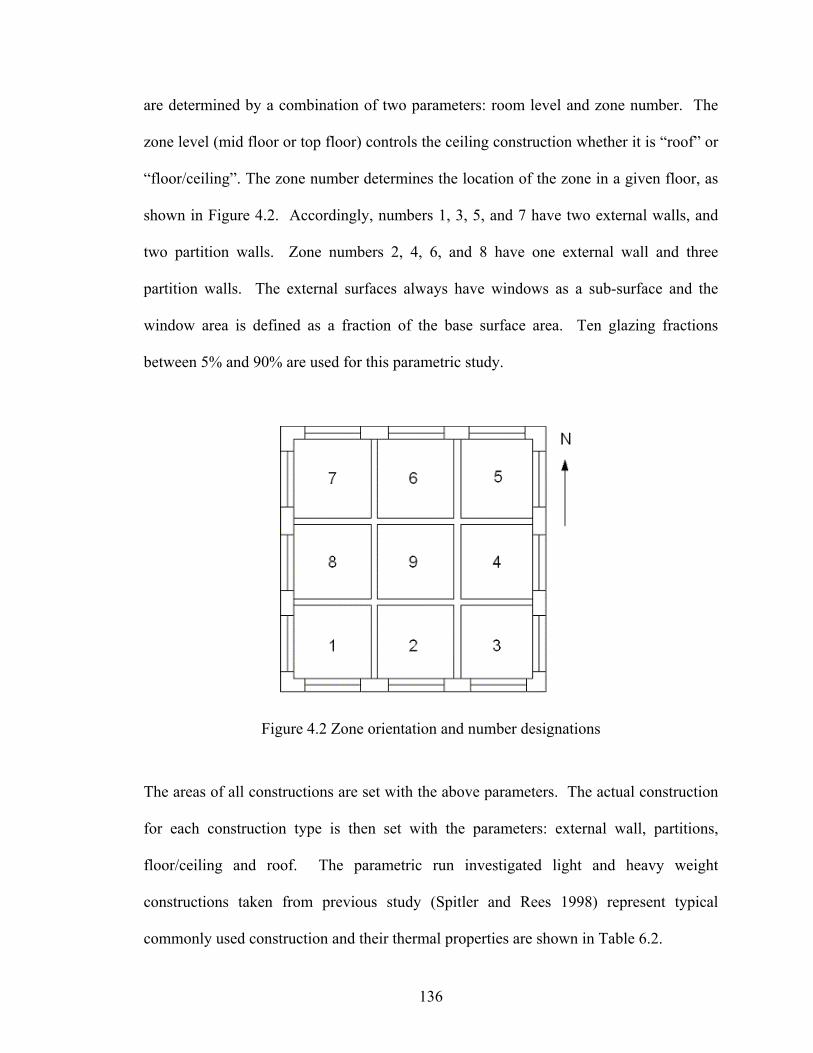
136
are determined by a combination of two parameters: room level and zone number. The
zone level (mid floor or top floor) controls the ceiling construction whether it is “roof” or
“floor/ceiling”. The zone number determines the location of the zone in a given floor, as
shown in Figure 4.2. Accordingly, numbers 1, 3, 5, and 7 have two external walls, and
two partition walls. Zone numbers 2, 4, 6, and 8 have one external wall and three
partition walls. The external surfaces always have windows as a sub-surface and the
window area is defined as a fraction of the base surface area. Ten glazing fractions
between 5% and 90% are used for this parametric study.
Figure 4.2 Zone orientation and number designations
The areas of all constructions are set with the above parameters. The actual construction
for each construction type is then set with the parameters: external wall, partitions,
floor/ceiling and roof. The parametric run investigated light and heavy weight
constructions taken from previous study (Spitler and Rees 1998) represent typical
commonly used construction and their thermal properties are shown in Table 6.2.
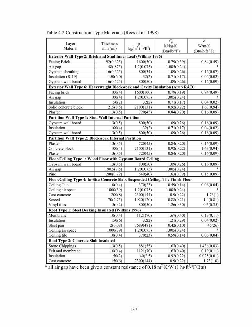
137
Table 4.2 Construction Type Materials (Rees et al. 1998)
Layer Material
Thickness mm (in.)
ρ kg/m3 (lb/ft3)
Cp kJ/kg⋅K
(Btu/lb⋅°F)
k W/m⋅K
(Btu/h⋅ft⋅°F) Exterior Wall Type 2: Brick and Stud Inner Leaf (Wilkins 1996) Facing Brick 92(0.625) 1600(50) 0.79(0.39) 0.84(0.49)Air gap 48(.875) 1.2(0.075) 1.005(0.24) *Gypsum sheathing 16(0.625) 800(34) 1.09(0.26) 0.16(0.07)Insulation (R-19) 150(6.0) 32(2) 0.71(0.17) 0.04(0.02)Gypsum wall board 16(0.625) 800(50) 1.09(0.26) 0.16(0.09)Exterior Wall Type 6: Heavyweight Blockwork and Cavity Insulation (Arup R&D) Facing brick 100(4) 1600(100) 0.79(0.19) 0.84(0.49)Air gap 100(4) 1.2(0.075) 1.005(0.24) *Insulation 50(2) 32(2) 0.71(0.17) 0.04(0.02)Solid concrete block 215(8.5) 2100(131) 0.92(0.22) 1.63(0.94)Plaster 13(0.5) 720(45) 0.84(0.20) 0.16(0.09)Partition Wall Type 1: Stud Wall Internal Partition Gypsum wall board 13(0.5) 800(50) 1.09(0.26) 0.16(0.09)Insulation 100(4) 32(2) 0.71(0.17) 0.04(0.02)Gypsum wall board 13(0.5) 800(50) 1.09(0.26) 0.16(0.09)Partition Wall Type 2: Blockwork Internal Partition Plaster 13(0.5) 720(45) 0.84(0.20) 0.16(0.09)Concrete block 100(4) 2100(131) 0.92(0.22) 1.63(0.94)Plaster 13(0.5) 720(45) 0.84(0.20) 0.16(0.09)Floor/Ceiling Type 1: Wood Floor with Gypsum Board Ceiling Gypsum wall board 13(0.5) 800(50) 1.09(0.26) 0.16(0.09)Air gap 190.5(7.5) 1.2(0.075) 1.005(0.24) *Pine 200(0.79) 640(40) 1.63(0.39) 0.15(0.09)Floor/Ceiling Type 4: In-Situ Concrete Slab, Suspended Ceiling, Tile Finish Floor Ceiling Tile 10(0.4) 370(23) 0.59(0.14) 0.06(0.04)Ceiling air space 1000(39) 1.2(0.075) 1.005(0.24) *Cast concrete 200(8) 2300(144) 0.9(0.22) 1.73(1)Screed 70(2.75) 1920(120) 0.88(0.21) 1.4(0.81)Vinyl tiles 5(0.2) 800(50) 1.26(0.30) 0.6(0.35)Roof Type 1: Steel Decking Insulated (Wilkins 1996) Membrane 10(0.4) 1121(70) 1.67(0.40) 0.19(0.11)Insulation 150(6) 32(2) 1.21(0.29) 0.04(0.02)Steel pan 2(0.08) 7689(481) 0.42(0.10) 45(26)Ceiling air space 1000(39) 1.2(0.075) 1.005(0.24) *Ceiling tile 10(0.4) 370(23) 0.59(0.14) 0.06(0.04)Roof Type 2: Concrete Slab Insulated Stone Chippings 13(0.5) 881(55) 1.67(0.40) 1.436(0.83)Felt and membrane 10(0.4) 1121(70) 1.67(0.40) 0.19(0.11)Insulation 50(2) 40(2.5) 0.92(0.22) 0.025(0.01)Cast concrete 150(6) 2300(144) 0.9(0.22) 1.73(1.0)
* all air gap have been give a constant resistance of 0.18 m2⋅K/W (1 hr⋅ft2⋅ºF/Btu)
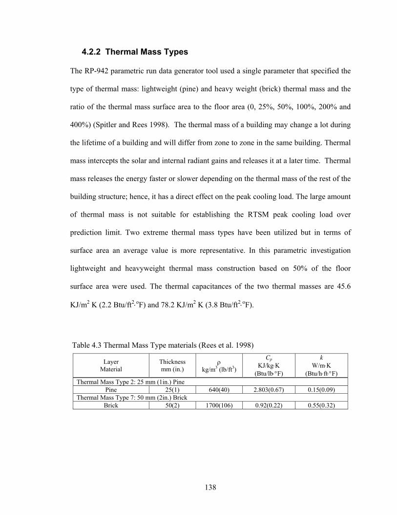
138
4.2.2 Thermal Mass Types
The RP-942 parametric run data generator tool used a single parameter that specified the
type of thermal mass: lightweight (pine) and heavy weight (brick) thermal mass and the
ratio of the thermal mass surface area to the floor area (0, 25%, 50%, 100%, 200% and
400%) (Spitler and Rees 1998). The thermal mass of a building may change a lot during
the lifetime of a building and will differ from zone to zone in the same building. Thermal
mass intercepts the solar and internal radiant gains and releases it at a later time. Thermal
mass releases the energy faster or slower depending on the thermal mass of the rest of the
building structure; hence, it has a direct effect on the peak cooling load. The large amount
of thermal mass is not suitable for establishing the RTSM peak cooling load over
prediction limit. Two extreme thermal mass types have been utilized but in terms of
surface area an average value is more representative. In this parametric investigation
lightweight and heavyweight thermal mass construction based on 50% of the floor
surface area were used. The thermal capacitances of the two thermal masses are 45.6
KJ/m2 K (2.2 Btu/ft2⋅oF) and 78.2 KJ/m2 K (3.8 Btu/ft2⋅oF).
Table 4.3 Thermal Mass Type materials (Rees et al. 1998)
Layer Material
Thickness mm (in.)
ρ kg/m3 (lb/ft3)
Cp KJ/kg⋅K
(Btu/lb⋅°F)
k W/m⋅K
(Btu/h⋅ft⋅°F) Thermal Mass Type 2: 25 mm (1in.) Pine
Pine 25(1) 640(40) 2.803(0.67) 0.15(0.09) Thermal Mass Type 7: 50 mm (2in.) Brick
Brick 50(2) 1700(106) 0.92(0.22) 0.55(0.32)
139
4.2.3 Internal Heat Gains and Schedules
People, lighting and equipment loads were included in the parametric investigation by
defining the zone peak heat gain loading. Then the hourly heat gain rates are determined
by multiplying the peak heat gain and the 24-hourly heat gain schedules. The parametric
run generation tool has six schedule types but only two have been used in this
investigation. For the base case analysis the following internal heat gain values were
used: 10 people per 100m2 for people, 20 W/m2 (6.34 Btu/h⋅ft2) for lighting and 30 W/m2
(9.51 Btu/h⋅ft2) for equipment. Investigation attempted to quantitatively analyze internal
heat gain loading impact on the RTS method likely peak cooling load overprediction. It is
common practice to use constant radiative / convective split of internal heat gains in
RTSM. ASHRAE 942-RP parametric runs generator uses a fixed radiative / convective
split for all parametric runs: 70/30 for people, 30/70 for equipment and 67/33 for lighting
heat gains. However, for quantitative characterization of the maximum RTSM peak
cooling load over prediction there is a need to consider wide range of radiative /
convective splits, which also depends on Luminaire type, the space air flow rate and
lighting input intensity.
ASHRAE’s RP-1282 provided lighting heat gain fractions based on experimental studies
on twelve luminaires types (Fisher and Chantrasrisalai, 2006). The RP-1282
recommended five luminaire categories for purposes of setting the radiative / convective
split. The recommended ranges were based on studies made on lighting heat input rates
in the range 0.9 W/ft2 (9.69 W/m2) to 2.6 W/ft2 (27.99 W/m2). A typical peak lighting
heat gain rate of 1.86 W/ft2 (20.0 W/m2) was used in this parametric investigation.
140
The equipment peak heat gain loading expected in commercial buildings ranges widely
and depends on the building usage. An electronic equipment heat gain load study made
on office buildings has shown that the actual load factor ranges between 0.32 W/ft2 (3.44
W/m2) to 1.33 W/ft2 (14.32 W/m2) and if the usage diversity is ignored the maximum
loading may reach 1.75 W/ft2 (18.8 W/m2) (Wilkins 1998). Average equipment heat gain
loading for medical center hospital laboratory spaces can be 6.71 W/ft2 (72.2 W/m2) and
it could be as high as 10.65 W/ft2 (114.6 W/m2) (Wilkins and Cook 1999). The
equipment load density is wide range depending on the building usage and industry
category; hence, 2.79 W/ft2 (30.0 W/m2) has been utilized as a representative typical
value over the entire range.
4.2.4 Glazing Types
In general the original RTSM tends to over predict the peak cooling load when the zone
has large amount of single pane glazing and exposed to lower outside design air
temperature. However, the RTSM peak cooling load overprediction decreases
substantially for double pane fenestration systems due to a decrease in conductance and
solar heat gain. Therefore, here it is intended to provide design guidance for four
categories of fenestration types: single pane clear window, double pane clear windows,
double pane low-emissivity glass windows and double pane reflective coated glass
windows shown in Table 6.4. The individual glass layer properties were taken from
LBNL Optics5 optical glazing database that closely duplicate the system properties given
in ASHRAE Handbook of Fundamental (ASHRAE 2005).

141
Table 4.4 Single Pane Clear Glass Window Glazing Type 1: Single Pane Clear Glass, Aluminum Frame (1b)
Layer Material Thickness Coating Clear Glass 0.24 in (6mm) None
U-factor 6.10 W/m2⋅oC 1.07 Btu/(h⋅ft2⋅oF)
Shading Coefficient 0.93 Normal SHGC 0.81 Normal Solar absorptance 0.16 Normal Solar Transmittance 0.76 Inside emissivity 0.84 Outside emissivity 0.84
Surface-to-surface thermal conductance 151.7 W/m2⋅oC 26.70 Btu/(h⋅ft2⋅oF)
Glazing Type 2: Double glazing, Aluminum Frame with thermal break (5a)
Layer Material Thickness Coating Clear Glass 0.24 in (3 mm) None Air gap ½ in (12.7mm) Clear glass 0.24 in (3 mm) None
U-factor 2.86 W/m2⋅oC 0.50 Btu/(h⋅ft2⋅oF
Shading Coefficient 0.88 Normal SHGC 0.76 Normal Solar absorptance 0.17 Normal Solar Transmittance 0.70 Inside emissivity 0.84 Outside emissivity 0.84
Surface-to-surface thermal conductance 5.41 W/m2⋅oC 0.95 Btu/(h⋅ft2⋅oF)
Glazing Type 3: Double glazing, Tinted Low-E Coating, Aluminum Frame with thermal break (21f)
Layer Material Thickness Coating Bronze 0.24 in (3mm) None Air gap ½ in (12.7mm) Clear glass 0.24 in (3mm) Low-E
U-factor 1.76 W/m2⋅oC 0.31 Btu/(h⋅ft2⋅oF
Shading Coefficient 0.75 Normal SHGC 0.65 Normal Solar absorptance 0.27 Normal Solar Transmittance 0.59 Inside emissivity 0.84 Outside emissivity 0.84
Surface-to-surface thermal conductance 2.48 W/m2⋅oC 0.44 Btu/(h⋅ft2⋅oF)
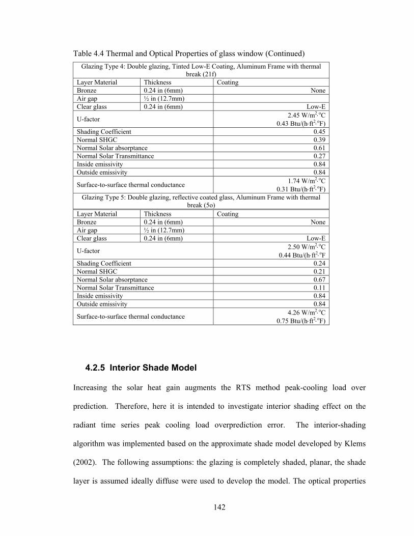
142
Table 4.4 Thermal and Optical Properties of glass window (Continued) Glazing Type 4: Double glazing, Tinted Low-E Coating, Aluminum Frame with thermal
break (21f) Layer Material Thickness Coating Bronze 0.24 in (6mm) None Air gap ½ in (12.7mm) Clear glass 0.24 in (6mm) Low-E
U-factor 2.45 W/m2⋅oC 0.43 Btu/(h⋅ft2⋅oF)
Shading Coefficient 0.45 Normal SHGC 0.39 Normal Solar absorptance 0.61 Normal Solar Transmittance 0.27 Inside emissivity 0.84 Outside emissivity 0.84
Surface-to-surface thermal conductance 1.74 W/m2⋅oC 0.31 Btu/(h⋅ft2⋅oF)
Glazing Type 5: Double glazing, reflective coated glass, Aluminum Frame with thermal break (5o)
Layer Material Thickness Coating Bronze 0.24 in (6mm) None Air gap ½ in (12.7mm) Clear glass 0.24 in (6mm) Low-E
U-factor 2.50 W/m2⋅oC 0.44 Btu/(h⋅ft2⋅oF
Shading Coefficient 0.24 Normal SHGC 0.21 Normal Solar absorptance 0.67 Normal Solar Transmittance 0.11 Inside emissivity 0.84 Outside emissivity 0.84
Surface-to-surface thermal conductance 4.26 W/m2⋅oC 0.75 Btu/(h⋅ft2⋅oF)
4.2.5 Interior Shade Model
Increasing the solar heat gain augments the RTS method peak-cooling load over
prediction. Therefore, here it is intended to investigate interior shading effect on the
radiant time series peak cooling load overprediction error. The interior-shading
algorithm was implemented based on the approximate shade model developed by Klems
(2002). The following assumptions: the glazing is completely shaded, planar, the shade
layer is assumed ideally diffuse were used to develop the model. The optical properties
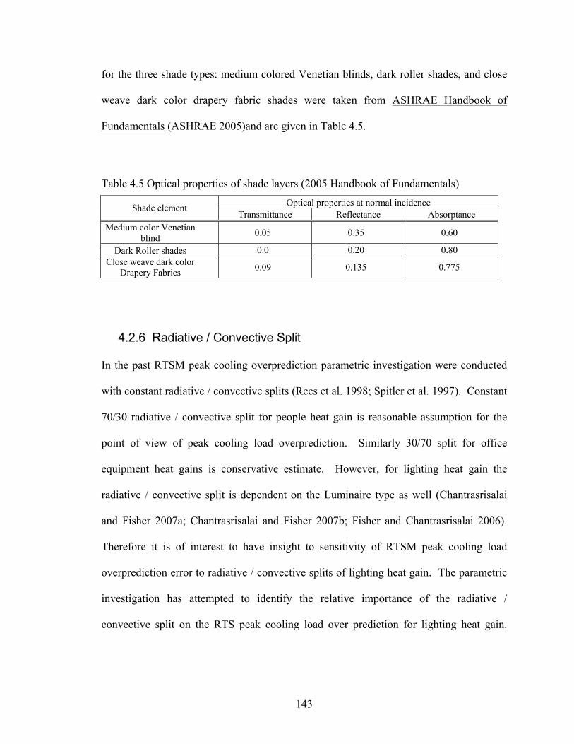
143
for the three shade types: medium colored Venetian blinds, dark roller shades, and close
weave dark color drapery fabric shades were taken from ASHRAE Handbook of
Fundamentals (ASHRAE 2005)and are given in Table 4.5.
Table 4.5 Optical properties of shade layers (2005 Handbook of Fundamentals) Optical properties at normal incidence Shade element
Transmittance Reflectance Absorptance Medium color Venetian
blind 0.05 0.35 0.60
Dark Roller shades 0.0 0.20 0.80 Close weave dark color
Drapery Fabrics 0.09 0.135 0.775
4.2.6 Radiative / Convective Split
In the past RTSM peak cooling overprediction parametric investigation were conducted
with constant radiative / convective splits (Rees et al. 1998; Spitler et al. 1997). Constant
70/30 radiative / convective split for people heat gain is reasonable assumption for the
point of view of peak cooling load overprediction. Similarly 30/70 split for office
equipment heat gains is conservative estimate. However, for lighting heat gain the
radiative / convective split is dependent on the Luminaire type as well (Chantrasrisalai
and Fisher 2007a; Chantrasrisalai and Fisher 2007b; Fisher and Chantrasrisalai 2006).
Therefore it is of interest to have insight to sensitivity of RTSM peak cooling load
overprediction error to radiative / convective splits of lighting heat gain. The parametric
investigation has attempted to identify the relative importance of the radiative /
convective split on the RTS peak cooling load over prediction for lighting heat gain.
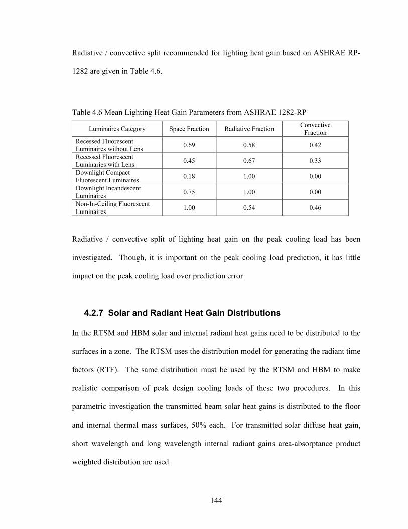
144
Radiative / convective split recommended for lighting heat gain based on ASHRAE RP-
1282 are given in Table 4.6.
Table 4.6 Mean Lighting Heat Gain Parameters from ASHRAE 1282-RP
Luminaires Category Space Fraction Radiative Fraction Convective Fraction
Recessed Fluorescent Luminaires without Lens 0.69 0.58 0.42
Recessed Fluorescent Luminaries with Lens 0.45 0.67 0.33
Downlight Compact Fluorescent Luminaires 0.18 1.00 0.00
Downlight Incandescent Luminaires 0.75 1.00 0.00
Non-In-Ceiling Fluorescent Luminaires 1.00 0.54 0.46
Radiative / convective split of lighting heat gain on the peak cooling load has been
investigated. Though, it is important on the peak cooling load prediction, it has little
impact on the peak cooling load over prediction error
4.2.7 Solar and Radiant Heat Gain Distributions
In the RTSM and HBM solar and internal radiant heat gains need to be distributed to the
surfaces in a zone. The RTSM uses the distribution model for generating the radiant time
factors (RTF). The same distribution must be used by the RTSM and HBM to make
realistic comparison of peak design cooling loads of these two procedures. In this
parametric investigation the transmitted beam solar heat gains is distributed to the floor
and internal thermal mass surfaces, 50% each. For transmitted solar diffuse heat gain,
short wavelength and long wavelength internal radiant gains area-absorptance product
weighted distribution are used.
145
4.2.8 Design Weather Days
In the RTSM the RTF are generated assuming adiabatic zone. The adiabatic boundary
condition is one of the inherent limiting assumptions of the RTSM. On the other hand,
the HBM models the building envelope interaction realistically by solving the inside and
outside surfaces heat balance equations along with zone air heat balance equations
simultaneously using the actual weather data as boundary conditions. Therefore, the
RTSM peak-cooling load over prediction shows sensitivities to the peak design outdoor
air temperature. Higher design weather temperature (relative to the room design
temperature) tends to offset parts of effects of the adiabatic boundary condition
assumption; hence, results in smaller RTS peak cooling load over prediction. On the
other hand, colder design weather tends to yield higher RTSM peak cooling load over
prediction. The RTSM peak cooling load overprediction error also varies across the year
primarily due to variation of the peak design temperature and intensity of solar incident.
The time of occurrence of annual peak design cooling load depends on many design
parameters primarily on: window glazing fraction, fenestration type, construction type,
zone orientation, site location, design weather conditions, internal heat gain loadings and
infiltration. Mostly for variety of design weather and zone locations the annual peak
design cooling load occurs from June to September, but for south facing zones with large
amount of glazing for lower end of the latitude angles of the USA locations such as:
Atlanta, and Miami with warm winter weather the annual peak design cooling load may
occur in November and December due to low solar elevation angles. Fourteen USA
representative climate regions were selected for this investigation. Each location uses the
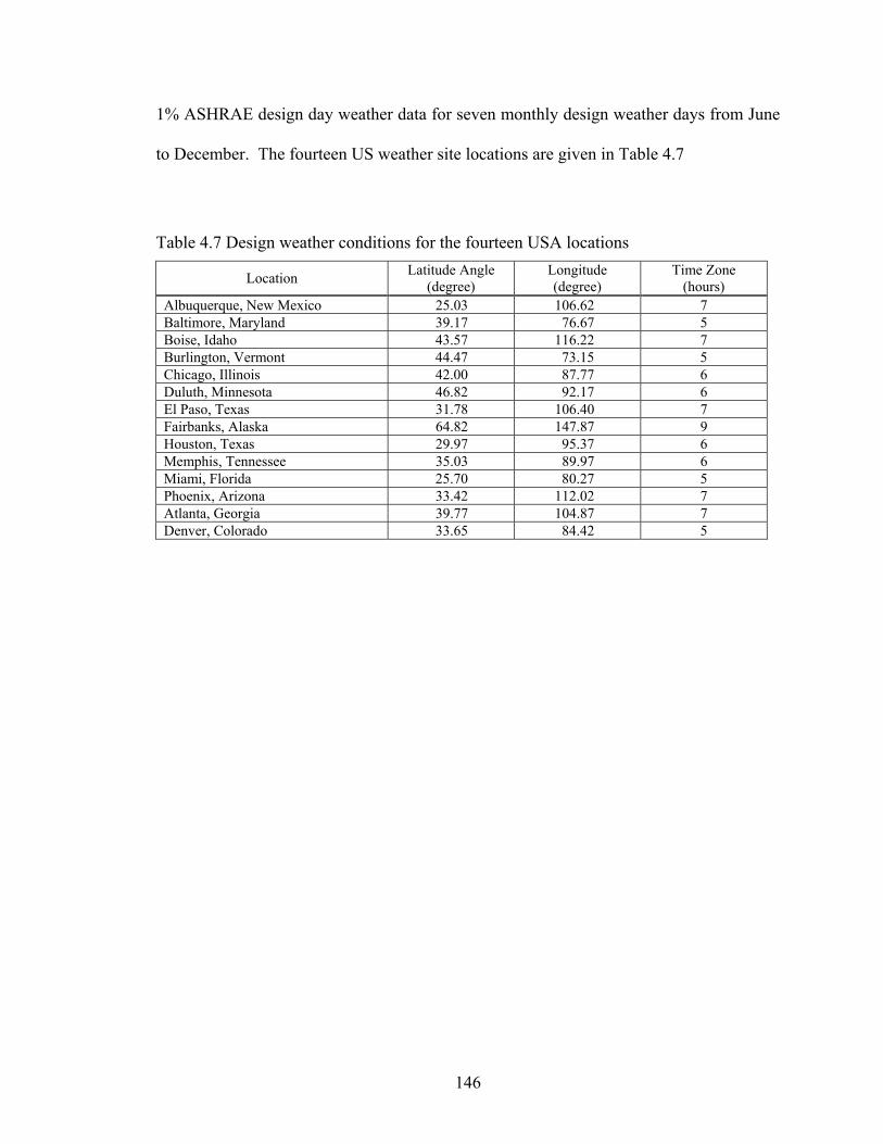
146
1% ASHRAE design day weather data for seven monthly design weather days from June
to December. The fourteen US weather site locations are given in Table 4.7
Table 4.7 Design weather conditions for the fourteen USA locations
Location Latitude Angle (degree)
Longitude (degree)
Time Zone (hours)
Albuquerque, New Mexico 25.03 106.62 7 Baltimore, Maryland 39.17 76.67 5 Boise, Idaho 43.57 116.22 7 Burlington, Vermont 44.47 73.15 5 Chicago, Illinois 42.00 87.77 6 Duluth, Minnesota 46.82 92.17 6 El Paso, Texas 31.78 106.40 7 Fairbanks, Alaska 64.82 147.87 9 Houston, Texas 29.97 95.37 6 Memphis, Tennessee 35.03 89.97 6 Miami, Florida 25.70 80.27 5 Phoenix, Arizona 33.42 112.02 7 Atlanta, Georgia 39.77 104.87 7 Denver, Colorado 33.65 84.42 5
147
4.3 Methodology: HBM and RTSM Implementation The purpose of this parametric investigation is to come up with quantitative
characterization of the original RTSM peak cooling load likely overprediction trend
compared to the HBM, which uses the most rigorous and fundamental mathematic
algorithms. It is not straightforward task to generalize the RTSM peak-cooling load
over prediction error when it depends on several building design parameters. Therefore it
of interest to define the RTSM peak design cooling loads over prediction error. Here it is
defined as the deviation of the RTSM annual peak design-cooling load from that of the
HBM. The annual peak design-cooling load is taken as the maximum of the peak-cooling
load computed for the hot months of the year from June to December. In the RTSM as a
load calculation procedure we are interested on the annual peak design cooling loads.
Thus, to encompass possible design conditions the annual peak design cooling loads of
the RTSM and HBM were computed for a wide range and different combination of
nineteen building design parameters.
The RTSM annual peak design cooling load overprediction error were determined using
fully populated parametric run to establish the general overprediction trend for a range of
building design parameter such as: glazing type, glazing fraction, design weather, zone
location, construction fabric, internal heat gains, schedules, infiltration rates, furniture
thermal mass and aspect ratio and interior shades. Furthermore, sensitivity of the
maximum error of the RTS annual peak design-cooling load was investigated for other
design parameters: internal heat gain rates, radiative / convective split, carpeting and
interior shade effects. The following section describes the basic features and component
models of the HBM and RTSM utilized in the parametric run tool.
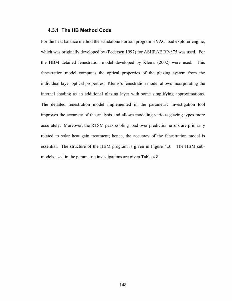
148
4.3.1 The HB Method Code
For the heat balance method the standalone Fortran program HVAC load explorer engine,
which was originally developed by (Pedersen 1997) for ASHRAE RP-875 was used. For
the HBM detailed fenestration model developed by Klems (2002) were used. This
fenestration model computes the optical properties of the glazing system from the
individual layer optical properties. Klems’s fenestration model allows incorporating the
internal shading as an additional glazing layer with some simplifying approximations.
The detailed fenestration model implemented in the parametric investigation tool
improves the accuracy of the analysis and allows modeling various glazing types more
accurately. Moreover, the RTSM peak cooling load over prediction errors are primarily
related to solar heat gain treatment; hence, the accuracy of the fenestration model is
essential. The structure of the HBM program is given in Figure 4.3. The HBM sub-
models used in the parametric investigations are given Table 4.8.
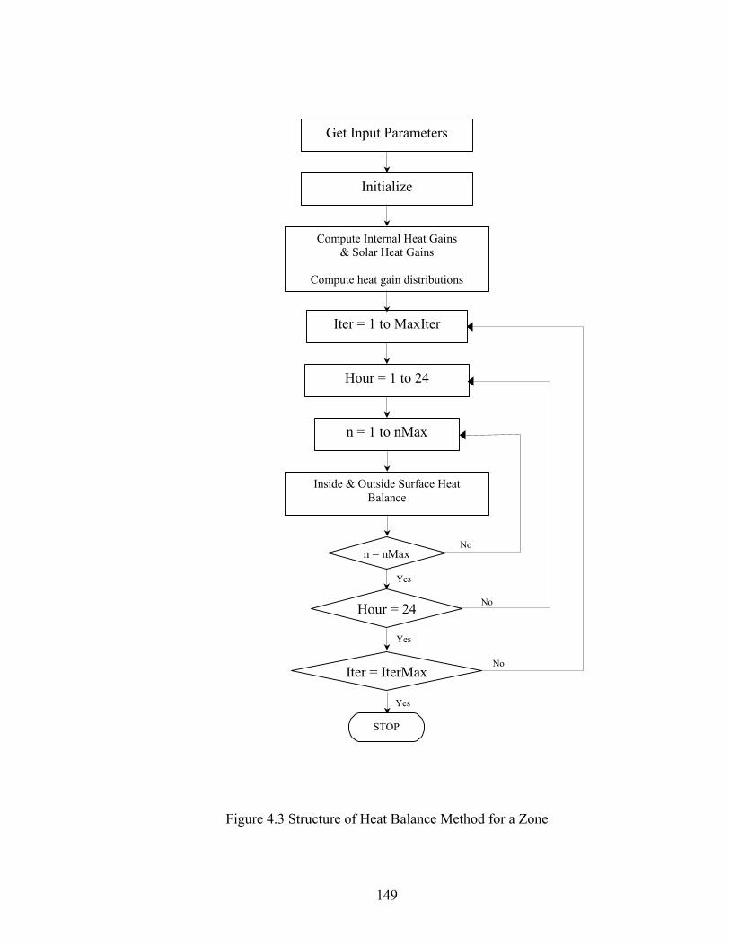
149
Get Input Parameters
Initialize
Compute Internal Heat Gains & Solar Heat Gains
Compute heat gain distributions
Inside & Outside Surface Heat Balance
Iter = 1 to MaxIter
Hour = 1 to 24
n = 1 to nMax
n = nMax
Hour = 24
Iter = IterMax
No
No
No
STOP
Yes
Yes
Yes
Figure 4.3 Structure of Heat Balance Method for a Zone
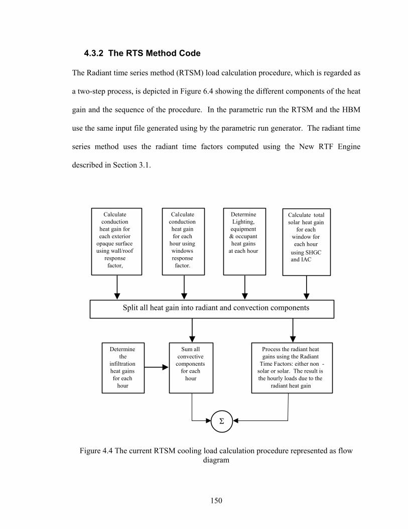
150
4.3.2 The RTS Method Code
The Radiant time series method (RTSM) load calculation procedure, which is regarded as
a two-step process, is depicted in Figure 6.4 showing the different components of the heat
gain and the sequence of the procedure. In the parametric run the RTSM and the HBM
use the same input file generated using by the parametric run generator. The radiant time
series method uses the radiant time factors computed using the New RTF Engine
described in Section 3.1.
Determine Lighting,
equipment & occupant heat gains
at each hour
Calculate conduction heat gain for each
hour using windows response factor.
Calculate conduction
heat gain for each exterior
opaque surface using wall/roof
response factor,
Split all heat gain into radiant and convection components
Determine the
infiltration heat gains for each
hour
Sum all convective
components for each
hour
Process the radiant heat gains using the Radiant
Time Factors: either non - solar or solar. The result is the hourly loads due to the
radiant heat gain
Σ
Calculate total solar heat gain
for each window for each hour
using SHGC and IAC
Figure 4.4 The current RTSM cooling load calculation procedure represented as flow
diagram

151
4.3.3 The RTSM and HBM Models Comparison
The heat balance and radiant time series methods use component model to represents the
different physical processes in the zone models. The major component models for the
HBM and RTSM are described in Table 4.8.
152
Table 4.8 RTSM and HBM component models
Models HBM RTF Generation RTSM Solar Irradiance ASHRAE clear sky model - ASHRAE clear sky model
Internal Solar Distribution
Beam Solar: 50% to the floor and 50% to the furniture. Diffuse Solar: area-absorptance product weighted.
Beam Solar: 50% to the floor and 50% to the furniture.
Solar-RTF
Internal Radiant Gain Distribution
Short and Longwave radiation: area-absorptance product weighted.
area-absorptance product weighted. Non-solar RTF
Outside Boundary condition:
Outside air temperature. The ground surface assigned the outdoor air temperature. Blast sky temperature model.
- Sol-air temperature
Inside Convection Coefficients
Fixed coefficients: Walls: hc = 4.68 (W/m2 K)
Floor: hc = 4.37 (W/m2 K)
Ceiling: hc = 1.25 (W/m2 K)
Fixed coefficients: Walls: hc = 4.68 (W/m2 K)
Floor: hc = 4.37 (W/m2 K)
Ceiling: hc = 1.25 (W/m2 K)
Combined conductance hcombined = 8.3 (W/m2 K)
Outside Convection Coefficients hc = 17.03 (W/m2 K) - hcombined = 22.03 (W/m2 K)
Inside Longwave Radiation Model MRT / Balance (Walton, 1980) MRTNet (Carroll, 1980) Surfaces radiating to room air
Fenestration Model Detailed Model (Klems, 2002) - Solar Heat Gain Coefficient
Interior Shade Model Detailed Model (Klems, 2002) - Interior Attenuation Coefficients
153
4.4 Results and Discussion – Original RTSM
The objective of this chapter is to examine the RTSM annual peak design cooling load
prediction performance relative to the HBM using parametric run tool over wide range
and combinations of nineteen different building design parameters shown in Table 6.1.
The parametric values and level were selected based on typical design values for internal
heat gains, schedules, aspect ratio and glazing types, light and heavyweight for
construction fabrics, and exterior facade glazing fractions. Furthermore, detailed
parametric investigation of the effect of internal heat gain rates and radiative / convective
splits for lighting heat gains was conducted.
The RTSM annual peak design cooling load error was established based 376,320 cases of
parametric runs for each of the glazing types investigated. Seven months of design day
weather were used for each of the fourteen USA weather locations. The RTSM annual
peak design cooling load over prediction trend was investigated for typical internal heat
gain values (10 people per 100m2 occupancy level, 20 W/m2 light heat gain intensity and
30 W/m2 equipment heat gain loading) and fixed radiative / convective splits. The
original RTSM annual peak design cooling load error shows strong correlation to
building design parameters that lead to higher solar heat gain such as: glazing fraction of
exterior facade, glazing type, number of exterior facades, peak design temperatures, and
zone locations. The over prediction trend is also affected by the outdoor air design
temperature. Colder design weather increases the over prediction, and hotter design
weather tends to decrease the over prediction trend.
154
The annual peak design-cooling load for the most of the USA occurs in the months from
July to September. Though, some weather locations and zones with large glazing facing
south may peak in the months from October to December.
4.4.1 RTSM Peak Design Cooling Load Prediction
The RTSM annual peak cooling load over-prediction trend has been investigated, the
primary building design parameters contributing to the over prediction has been
examined, and the maximum annual peak design cooling load over prediction error of the
RTSM for the USA locations has been established.
The analysis presented here demonstrates the sensitivity of the RTSM annual peak
design-cooling load over prediction to the different building design parameters. Also
explains the relative importance of the design parameters to the RTSM peak-cooling load
over prediction. Then establishes the RTSM annual peak-cooling loads maximum over
predictions. The effects of building design parameters that have primary effect on the
RTSM peak cooling load over prediction: glazing fraction of exterior facade, glazing
type, number of exterior facades, peak design temperature, zone location, and
construction fabrics, are presented next.
RTSM over Prediction Sensitivity Analysis
The RTSM peak cooling load over prediction sensitivity to different building design
parameters has been investigated to establish extreme over prediction limits. The
sensitivity analysis helps to establish the relative importance of the building design
155
parameters on the RTSM over prediction. It has been established that RTSM cooling
load over prediction primarily depends on the treatment of solar and internal heat gains.
In the following analysis the relative contributions of the different building design
parameters to the peak cooling load over prediction error is presented.
Glazing Type
The effect of glazing type on the RTSM over prediction of peak cooling load is
demonstrated for a lightweight construction zone with exterior surface in north and east
facade for a building located in Atlanta, Georgia. The peak-cooling load over prediction
error differences between the glazing types progressively increases with glazing fraction.
The over prediction difference between single and double pane clear glasses for 90%
glazing fraction can be as much as 13.2%. Based on annual peak design cooling load for
Atlanta, Georgia, the extreme peak cooling over prediction for zones with two exterior
facades for single pane clear glazing is under 29% at 90% glazing fraction. The higher
peak cooling load over prediction error of the RTSM for single pane clear glazing is due
to large amount of solar heat gain and conservation of the entire heat gain. However, the
HBM may allow part of the radiant heat gain to be conducted back out depending on
glazing conductance and temperature difference between outside and inside air
temperature. Similar trend is observed for other locations as well but the extent of over
prediction depends on the outdoor air temperature for the same building design
parameters.
156
Number of Exterior Facades
The RTSM peak cooling load over prediction error has been examined using lightweight
construction zone with single exterior facade for single pane clear glass for two extreme
weather locations: Phoenix, Arizona, and Fairbanks, Alaska. The RTSM peak-cooling
load over prediction shows dependency on the zone exterior facade orientation for zones
with single exterior facade. In general zones facing east and west directions have higher
peak cooling load over prediction error compared to south and north facing zones due to
large amount of solar heat gains. Depending on the facing direction of the exterior faced
the RTSM peak cooling over prediction error may vary between 6 to 12% for zones with
single exterior surface at 90% glazing fraction for single pane clear glass. The peak
cooling load over prediction for locations with warm design weather condition like
Phoenix, Arizona is less by as much as 5% compared to colder design weather location
like Fairbanks, Alaska for zones with east and west exterior facades. In the case of zones
with south facing exterior facades the over prediction is strongly dependent on the
latitude angle as well. Phoenix, which has warm design weather the RTSM over
prediction, is less from that of Fairbanks by 2% only. In Fairbanks, Alaska, south facing
zones have their peak-cooling load in July. The north facing zones generally has the least
peak-cooling load over prediction error compared to any other orientations for zones with
single exterior facade.
Peak Design Temperature and Latitude
The RTSM peak-cooling load over prediction also depends on the peak design
temperature. The RTSM peak-cooling load depends on the difference between the
157
outdoor air and indoor air temperatures. In general lower peak design temperatures have
higher peak cooling load over prediction error. For zones with two exterior facades the
effect of peak design temperature may bring as much as 6% difference on the peak
cooling load over prediction between the warmest and coldest summer cooling design
weather conditions for the USA for 90% exterior facade glazing fraction. The latitude
affects the amount of solar heat gain and hence the RTSM peak cooling loads over
prediction error but has secondary effect for zones with two exterior facades. Zones with
two adjacent exterior facades the RTSM annual peak design cooling loads over prediction
primarily depends on peak design temperature. Peak cooling load over predictions are
almost the same for locations with similar design weather conditions but the amount of
peak cooling could be different. For instance for a north east zone in Chicago and
Atlanta with peak design temperatures of 35.8°C and 34.8°C for the month of July,
respectively, their RTSM annual peak cooling load over prediction error closely match at
all glazing fractions though there is significant latitude difference.
Construction Fabrics
The RTSM peak-cooling load over prediction has been investigated for lightweight and
heavyweight construction zones with single pane clear glazing. On average for the
original RTSM peak-cooling load lightweight construction zones over predicted by as
much as 3% to 4% higher than that of the heavyweight lightweight construction zones.
158
The sensitivity analysis has shown that the RTSM annual design peak cooling load over
prediction error primarily depends on: glazing fraction, glazing type, zone orientation,
number of exterior surfaces, peak design temperature, and construction fabric. The
former four building design parameters control the amount of solar heat gain. A
secondary effect dependency was also observed on internal heat gain schedule and
furnishing thermal mass.
The RTSM peak-cooling load for a given zone and weather location depends on the
month at which the load is calculated. The RTSM as peak load calculation procedure it
intended for sizing equipments and hence our primary interest should be the annual peak-
cooling load. In order to establish the maximum RTSM over prediction limit, the error
analysis should be based on the annual peak-cooling load. Therefore, the annual RTSM
peak cooling load needs to be determined for the fourteen USA weather locations. The
following section defines the basis for the annual peak cooling load calculation for the
different weather locations and typical design condition.
RTSM Annual Peak Design Cooling Load
The RTSM annual peak cooling load error sets the maximum design cooling load error
expected for a given design weather at annual peak design cooling load computed over a
range of combination of several building design parameters such as: zone location,
internal heat gain loadings, construction fabrics, fenestration type, glazing fractions of
exterior facade, infiltrations, schedules and aspect ratio. The annual peak design-cooling
load does not necessarily occur on the warmest month of the year. The combined effect
159
of peak design temperature, exterior faced orientation and latitude of the location
determines the peak cooling load and the time of occurrence. In particular for zones with
south facing exterior facade and for lower end latitude (e.g. Atlanta, Georgia, and
Phoenix, Arizona) that have warm winter design temperatures the peak cooling load may
occur in October and November. Table 4.9 shows the annual peak cooling load
occurrence months for zones with different orientation and number of exterior facades.
Some zones have multiple peak months depending on the glazing fractions.
Table 4.9 Month of Annual Peak Cooling Load for zones with single pane clear glass Annual Peak Cooling Load Months Site Location South East South West North East North West
Zone with two adjacent exterior facade Phoenix 7,8,9 7,8,9 7 6,7 Chicago 7,9 7,8 7 7 Atlanta 7,8,9 7,8,9 7 7 Fairbanks 7 7 6 6 Zone with single exterior facade Phoenix 9,10 7 6 7 Chicago 8,9,10 7 7 7 Atlanta 8,9,10,11 7 7 7 Fairbanks 7,8 6 6 6
In this investigation, the RTSM peak-cooling load errors were calculated based on annual
peak design cooling load for the fourteen USA locations. The original RTSM annual
peak-cooling load has been analyzed based on the combinations of the nineteen building
design parameters making a total of 376,320 cases parametric run for each glazing type.
The annual peak cooling load from the above data set is only fourteen locations, eight
zones and ten glazing fraction (making a total of 14x8x10 = 1120 cases). The parametric
run required is 1120 cases only but we cannot determine the annual peak cooling load
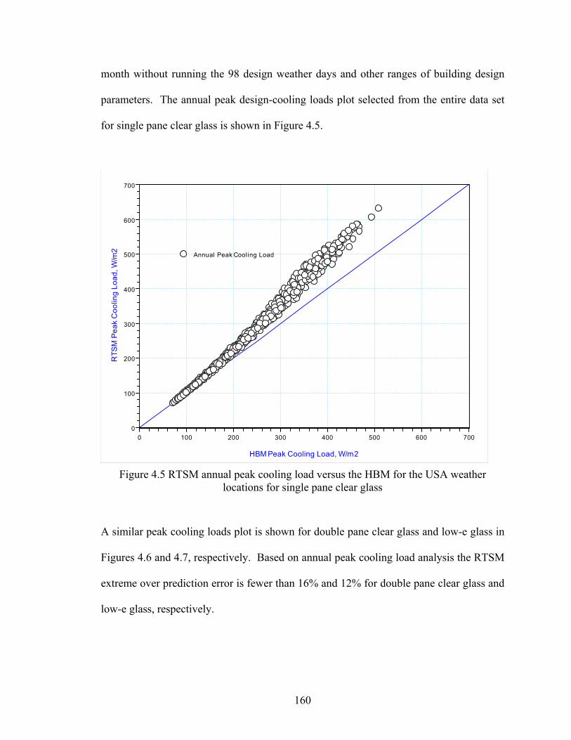
160
month without running the 98 design weather days and other ranges of building design
parameters. The annual peak design-cooling loads plot selected from the entire data set
for single pane clear glass is shown in Figure 4.5.
0 100 200 300 400 500 600 7000
100
200
300
400
500
600
700
HBM Peak Cooling Load, W/m2
RTS
M P
eak
Coo
ling
Load
, W/m
2
Annual Peak Cooling Load
Figure 4.5 RTSM annual peak cooling load versus the HBM for the USA weather
locations for single pane clear glass
A similar peak cooling loads plot is shown for double pane clear glass and low-e glass in
Figures 4.6 and 4.7, respectively. Based on annual peak cooling load analysis the RTSM
extreme over prediction error is fewer than 16% and 12% for double pane clear glass and
low-e glass, respectively.
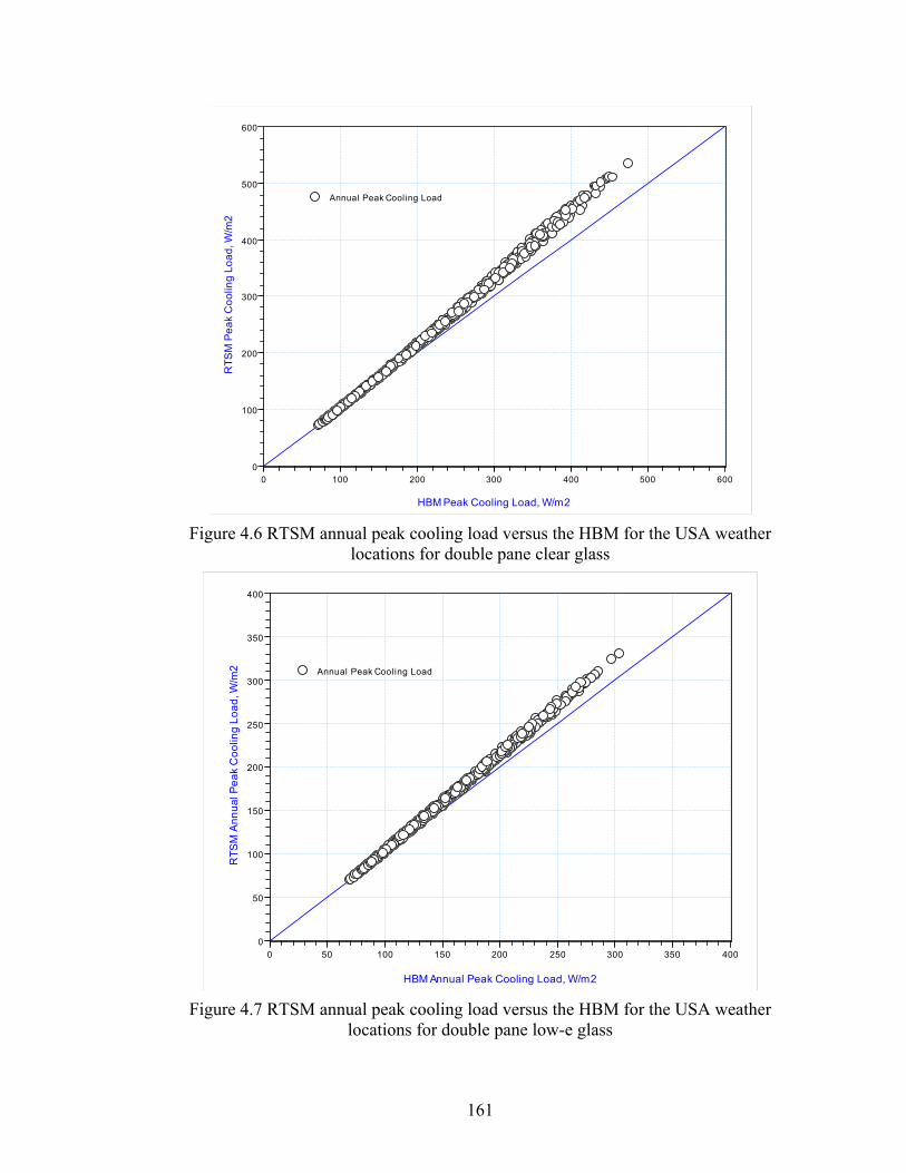
161
0 100 200 300 400 500 6000
100
200
300
400
500
600
HBM Peak Cooling Load, W/m2
RTS
M P
eak
Coo
ling
Load
, W/m
2
Annual Peak Cooling Load
Figure 4.6 RTSM annual peak cooling load versus the HBM for the USA weather
locations for double pane clear glass
0 50 100 150 200 250 300 350 4000
50
100
150
200
250
300
350
400
HBM Annual Peak Cooling Load, W/m2
RTS
M A
nnua
l Pea
k C
oolin
g Lo
ad, W
/m2 Annual Peak Cooling Load
Figure 4.7 RTSM annual peak cooling load versus the HBM for the USA weather
locations for double pane low-e glass
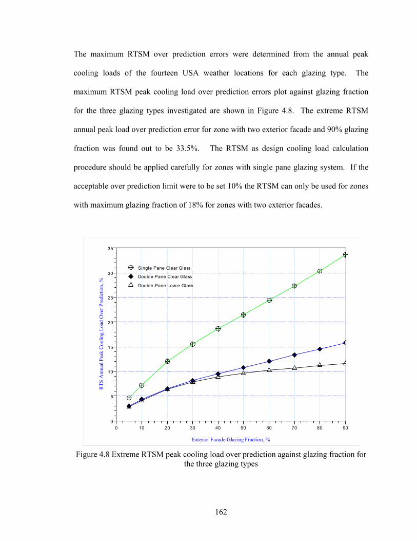
162
The maximum RTSM over prediction errors were determined from the annual peak
cooling loads of the fourteen USA weather locations for each glazing type. The
maximum RTSM peak cooling load over prediction errors plot against glazing fraction
for the three glazing types investigated are shown in Figure 4.8. The extreme RTSM
annual peak load over prediction error for zone with two exterior facade and 90% glazing
fraction was found out to be 33.5%. The RTSM as design cooling load calculation
procedure should be applied carefully for zones with single pane glazing system. If the
acceptable over prediction limit were to be set 10% the RTSM can only be used for zones
with maximum glazing fraction of 18% for zones with two exterior facades.
0 10 20 30 40 50 60 70 80 900
5
10
15
20
25
30
35
Exterior Facade Glazing Fraction, %
RTS
Ann
ual P
eak
Coo
ling
Load
Ove
r Pre
dict
ion,
%
Single Pane Clear Glass
Double Pane Clear Glass
Double Pane Low-e Glass
Figure 4.8 Extreme RTSM peak cooling load over prediction against glazing fraction for
the three glazing types
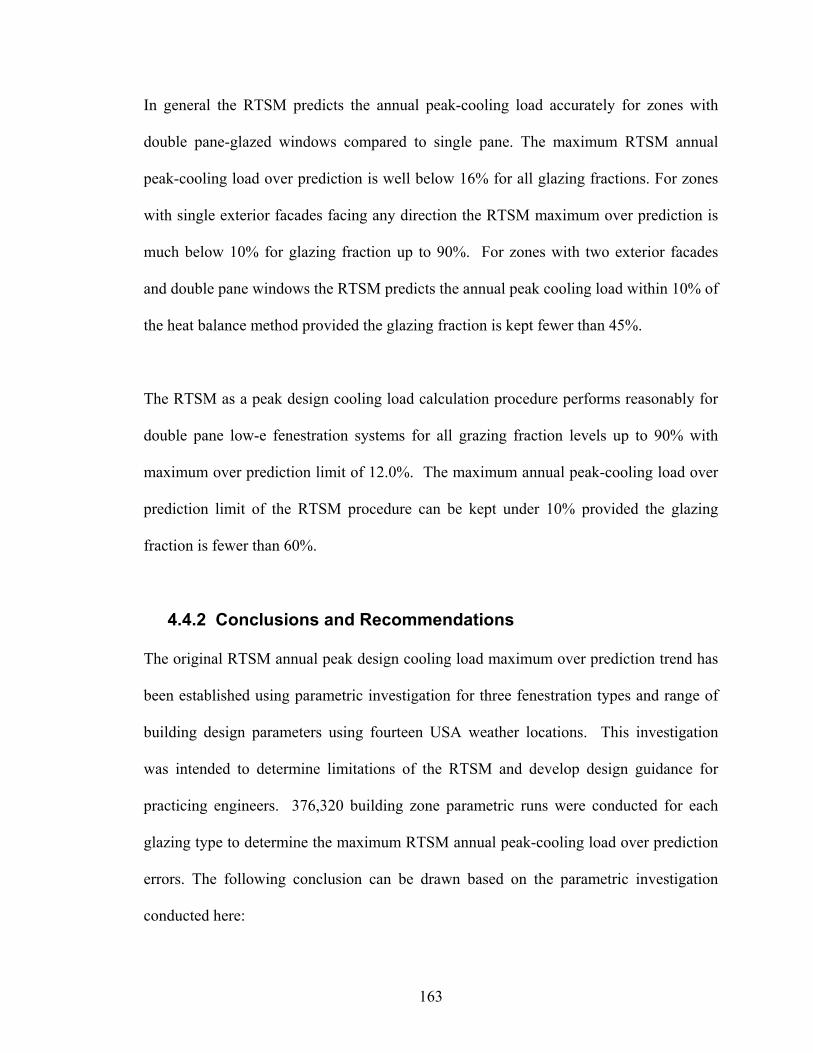
163
In general the RTSM predicts the annual peak-cooling load accurately for zones with
double pane-glazed windows compared to single pane. The maximum RTSM annual
peak-cooling load over prediction is well below 16% for all glazing fractions. For zones
with single exterior facades facing any direction the RTSM maximum over prediction is
much below 10% for glazing fraction up to 90%. For zones with two exterior facades
and double pane windows the RTSM predicts the annual peak cooling load within 10% of
the heat balance method provided the glazing fraction is kept fewer than 45%.
The RTSM as a peak design cooling load calculation procedure performs reasonably for
double pane low-e fenestration systems for all grazing fraction levels up to 90% with
maximum over prediction limit of 12.0%. The maximum annual peak-cooling load over
prediction limit of the RTSM procedure can be kept under 10% provided the glazing
fraction is fewer than 60%.
4.4.2 Conclusions and Recommendations
The original RTSM annual peak design cooling load maximum over prediction trend has
been established using parametric investigation for three fenestration types and range of
building design parameters using fourteen USA weather locations. This investigation
was intended to determine limitations of the RTSM and develop design guidance for
practicing engineers. 376,320 building zone parametric runs were conducted for each
glazing type to determine the maximum RTSM annual peak-cooling load over prediction
errors. The following conclusion can be drawn based on the parametric investigation
conducted here:
164
For the USA weather condition the maximum RTSM annual peak design cooling
load over prediction for zones having two adjacent exterior facades with 90%
glazing fraction single pane clear glass windows can be as much as 33.5%. This
corresponds to weather condition of the month of July in Fairbanks, Alaska. All
other locations, which have warmer design weather conditions over predict less.
For zones with single exterior facade either in the East or West facing direction
the maximum over prediction can only be as high as 26.0% for single pane clear
glass with 90% glazing. The maximum over prediction for zones with single
exterior facade viewing south or north and 90% glazing fraction can be as much
as 16.5% and 8.6%, respectively. Zones with single exterior faced facing south
can predict the annual design cooling load within 10% of the heat balance method
provided the single pane window glazing fraction is kept fewer than 75%. Zones
with east or west facing exterior facades for single pane glass windows the RTSM
can predict the annual peak design cooling load within 10% of the heat balance
method provided the glazing fraction is less than 35%. Similarly for zones with
two exterior facades the glazing fraction should be kept under 28%.
In general the RTSM performs well for double pane clear glass fenestration
systems. The RTS method over prediction of annual peak design cooling load is
below 12% for one and two exterior facades and glazing fraction levels up to
90%. For zones with two adjacent exterior facades and double pane clear glass
the RTSM can predict the annual peak design cooling within 11% of the heat
balance method if the glazing fraction is kept less than 50%. Zones with single
exterior facade viewing east or west the RTS method can predict the annual peak
165
cooling load within 9% of the heat balance method for glazing fractions up to
50%. Similarly zones with south or north facing exterior facades maximum over
prediction of annual peak cooling load by the RTS method is under 5% for all
glazing fraction levels up to 90%.
The RTSM over predicts the annual peak design cooling loads fewer than 11% for
zones with double pane low-e glazing up to 90% glazing fractions. The RTS
method maximum over prediction of the annual peak cooling load can be kept
under 10% for two exterior facade zones provided the glazing fraction is limited
to 55%. Zones with single exterior facade in the south and north facing direction
the RTS method predicts the annual peak cooling load by as much as 8.2% and
3.1%, respectively, for 90% glazing fractions.
The RTSM annual peak-cooling load over prediction correction factor has been
introduced. The correlation coefficients vary depending on number of exterior
facade and zone locations. The correction predicts the annual peak-cooling load
with ±6% of the heat balance method for single pane clear glass fenestration
system for two exterior facade zones.
Radiative / convective split of lighting heat gain on the peak cooling load has
been investigated. Though, it is important on the peak cooling load prediction, it
has little impact on the peak cooling load over prediction error.
166
4.5 Results and Discussion – Current and Improved RTSM
The performance of the current and improved RTSM procedures in predicting the peak
cooling loads has been established using wide range parametric runs and the
recommended radiative / convective splits given in Table 3.5. The maximum and
average peak cooling load over predictions for both current and improved RTSM
procedures has been established for use as a design guidance. The parametric
investigation has been run using the parameters range and levels given in Table 4.1. Four
sets of parametric runs were conducted – two for current RTSM and two for improved
RTSM. The two parametric runs for each procedure represent fenestration with and
without interior shades. The number of parametric runs for each test was limited to
716,800 zones to optimize the computational resource requirements. The nineteen
parameters combination for fenestration without interior shade include: four top floor
corner zones, two levels of construction fabrics one for lightweight and another for
heavyweight for each of surface constructions exterior (type 1 and type 6), partition (type
1 and type 2), roofs (type 1 and type 2) and floor surfaces (type 1 and type 4), five
glazing types, ten glazing fractions (5%, 10%, 20%, 30%, …, 90%), three aspect ratios
(0.5, 1.0 and 2.0), two levels of thermal mass (type 2 and type 7), two types of load
schedules (type 1 and type 6), and eight representative US weather locations (Burlington,
Chicago, Duluth, Fairbanks, Denver, Miami, Phoenix and Atlanta) with seven months of
design day data from June to December for each location making 56 design days weather.
The remaining parameters were: typical internal (people, lighting and equipment) heat
gain levels, typical infiltration rate of 0.5 ACH, and east-west axis size of 6m was used.
For the fenestration with interior shade a dark roller shade, which has zero transmittance,
167
was used. The dark roller shade was selected because it showed the highest tendency for
over prediction compared to the other two interior shades given in Table 4.4. A total of
2,867,200 test case parametric runs were conducted. Two sets of annual peak cooling
load were extracted for each of the four test cases – one for lightweight and another for
heavyweight. Each set has four zones, ten glazing fraction and eight locations making a
total of 320 annual peak cooling loads. The maximum over prediction for each glazing
type, construction type, glazing fraction and zone location / orientation were selected for
each of the four test cases to establish the maximum annual peak cooling load prediction
performance of the RTSM procedures. The next section presents the results for
fenestration without interior shades and then followed by fenestration with shades.
Application without Interior Shades
The RTSM peak cooling loads maximum and average over predictions for current and
improved procedures for zones without interior shaded fenestration have been established
are shown in Figures 4.9 and 4.10. For 716,800 zones without interior shaded
fenestration, the current RTSM procedure peak cooling over predictions can be as high as
30.5% while it is reduced to 10.5% for improved RTSM procedure. These occur for
zones with two exterior facades and with single pane clear glass at 90% glazing fraction.
The maximum and average over predictions were estimated from 71,680 zones for each
of the ten glazing fractions. The maximum over predictions for improved RTSM was
11.7%. This occurred for zones with two exterior façade surfaces, double pane reflected
coated glazing at 90% glazing fraction. Summary of the maximum over predictions for
the five glazing types without interior shades are given in Table 4.10.
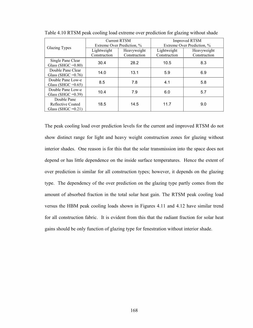
168
Table 4.10 RTSM peak cooling load extreme over prediction for glazing without shade Current RTSM
Extreme Over Prediction, % Improved RTSM
Extreme Over Prediction, % Glazing Types Lightweight Construction
Heavyweight Construction
Lightweight Construction
Heavyweight Construction
Single Pane Clear Glass (SHGC =0.80) 30.4 28.2 10.5 8.3
Double Pane Clear Glass (SHGC =0.76) 14.0 13.1 5.9 6.9
Double Pane Low-e Glass (SHGC =0.65) 8.5 7.8 4.1 5.8
Double Pane Low-e Glass (SHGC =0.39) 10.4 7.9 6.0 5.7
Double Pane Reflective Coated
Glass (SHGC =0.21) 18.5 14.5 11.7 9.0
The peak cooling load over prediction levels for the current and improved RTSM do not
show distinct range for light and heavy weight construction zones for glazing without
interior shades. One reason is for this that the solar transmission into the space does not
depend or has little dependence on the inside surface temperatures. Hence the extent of
over prediction is similar for all construction types; however, it depends on the glazing
type. The dependency of the over prediction on the glazing type partly comes from the
amount of absorbed fraction in the total solar heat gain. The RTSM peak cooling load
versus the HBM peak cooling loads shown in Figures 4.11 and 4.12 have similar trend
for all construction fabric. It is evident from this that the radiant fraction for solar heat
gains should be only function of glazing type for fenestration without interior shade.
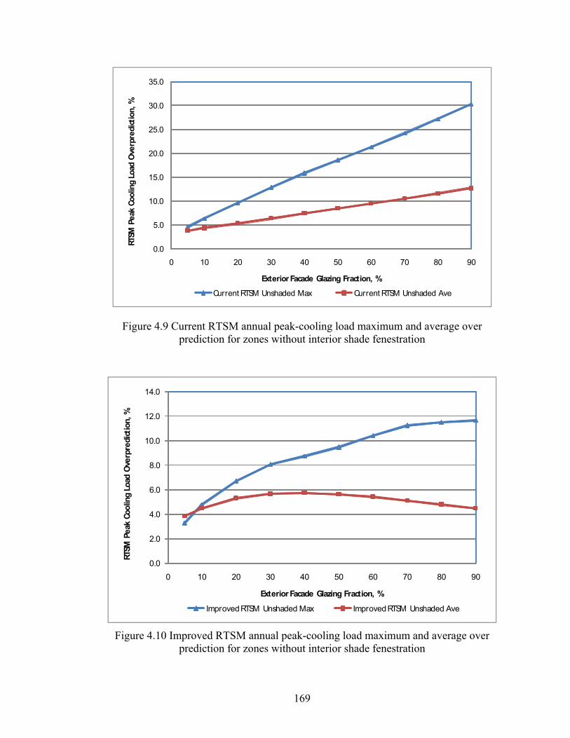
169
0.0
5.0
10.0
15.0
20.0
25.0
30.0
35.0
0 10 20 30 40 50 60 70 80 90
RTSM
Pea
k Co
olin
g Lo
ad O
verp
redi
ctio
n, %
Exterior Facade Glazing Fraction, %
Current RTSM Unshaded Max Current RTSM Unshaded Ave
Figure 4.9 Current RTSM annual peak-cooling load maximum and average over prediction for zones without interior shade fenestration
0.0
2.0
4.0
6.0
8.0
10.0
12.0
14.0
0 10 20 30 40 50 60 70 80 90
RTSM
Pea
k Co
olin
g Lo
ad O
verp
redi
ctio
n, %
Exterior Facade Glazing Fraction, %
Improved RTSM Unshaded Max Improved RTSM Unshaded Ave
Figure 4.10 Improved RTSM annual peak-cooling load maximum and average over prediction for zones without interior shade fenestration
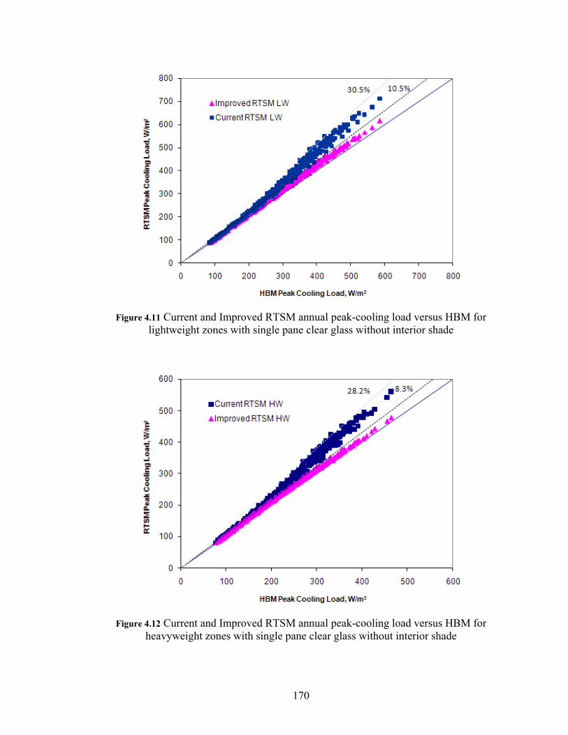
170
Figure 4.11 Current and Improved RTSM annual peak-cooling load versus HBM for
lightweight zones with single pane clear glass without interior shade
Figure 4.12 Current and Improved RTSM annual peak-cooling load versus HBM for
heavyweight zones with single pane clear glass without interior shade
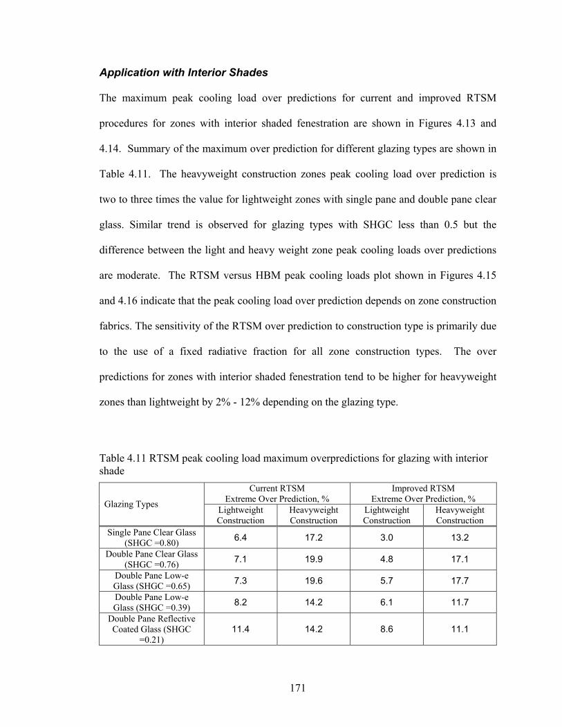
171
Application with Interior Shades
The maximum peak cooling load over predictions for current and improved RTSM
procedures for zones with interior shaded fenestration are shown in Figures 4.13 and
4.14. Summary of the maximum over prediction for different glazing types are shown in
Table 4.11. The heavyweight construction zones peak cooling load over prediction is
two to three times the value for lightweight zones with single pane and double pane clear
glass. Similar trend is observed for glazing types with SHGC less than 0.5 but the
difference between the light and heavy weight zone peak cooling loads over predictions
are moderate. The RTSM versus HBM peak cooling loads plot shown in Figures 4.15
and 4.16 indicate that the peak cooling load over prediction depends on zone construction
fabrics. The sensitivity of the RTSM over prediction to construction type is primarily due
to the use of a fixed radiative fraction for all zone construction types. The over
predictions for zones with interior shaded fenestration tend to be higher for heavyweight
zones than lightweight by 2% - 12% depending on the glazing type.
Table 4.11 RTSM peak cooling load maximum overpredictions for glazing with interior shade
Current RTSM Extreme Over Prediction, %
Improved RTSM Extreme Over Prediction, % Glazing Types Lightweight
Construction Heavyweight Construction
Lightweight Construction
Heavyweight Construction
Single Pane Clear Glass (SHGC =0.80) 6.4 17.2 3.0 13.2
Double Pane Clear Glass (SHGC =0.76) 7.1 19.9 4.8 17.1
Double Pane Low-e Glass (SHGC =0.65) 7.3 19.6 5.7 17.7
Double Pane Low-e Glass (SHGC =0.39) 8.2 14.2 6.1 11.7
Double Pane Reflective Coated Glass (SHGC
=0.21) 11.4 14.2 8.6 11.1
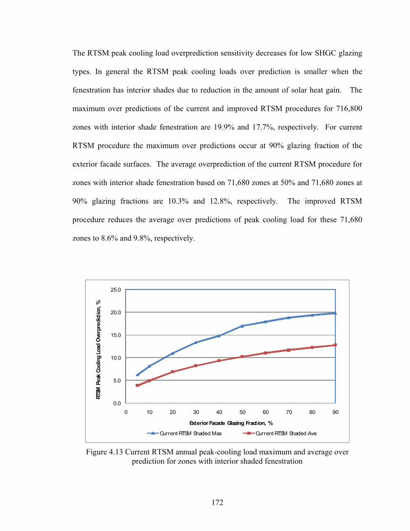
172
The RTSM peak cooling load overprediction sensitivity decreases for low SHGC glazing
types. In general the RTSM peak cooling loads over prediction is smaller when the
fenestration has interior shades due to reduction in the amount of solar heat gain. The
maximum over predictions of the current and improved RTSM procedures for 716,800
zones with interior shade fenestration are 19.9% and 17.7%, respectively. For current
RTSM procedure the maximum over predictions occur at 90% glazing fraction of the
exterior facade surfaces. The average overprediction of the current RTSM procedure for
zones with interior shade fenestration based on 71,680 zones at 50% and 71,680 zones at
90% glazing fractions are 10.3% and 12.8%, respectively. The improved RTSM
procedure reduces the average over predictions of peak cooling load for these 71,680
zones to 8.6% and 9.8%, respectively.
0.0
5.0
10.0
15.0
20.0
25.0
0 10 20 30 40 50 60 70 80 90
RTSM
Pea
k Co
olin
g Lo
ad O
verp
redi
ctio
n, %
Exterior Facade Glazing Fraction, %
Current RTSM Shaded Max Current RTSM Shaded Ave
Figure 4.13 Current RTSM annual peak-cooling load maximum and average over prediction for zones with interior shaded fenestration
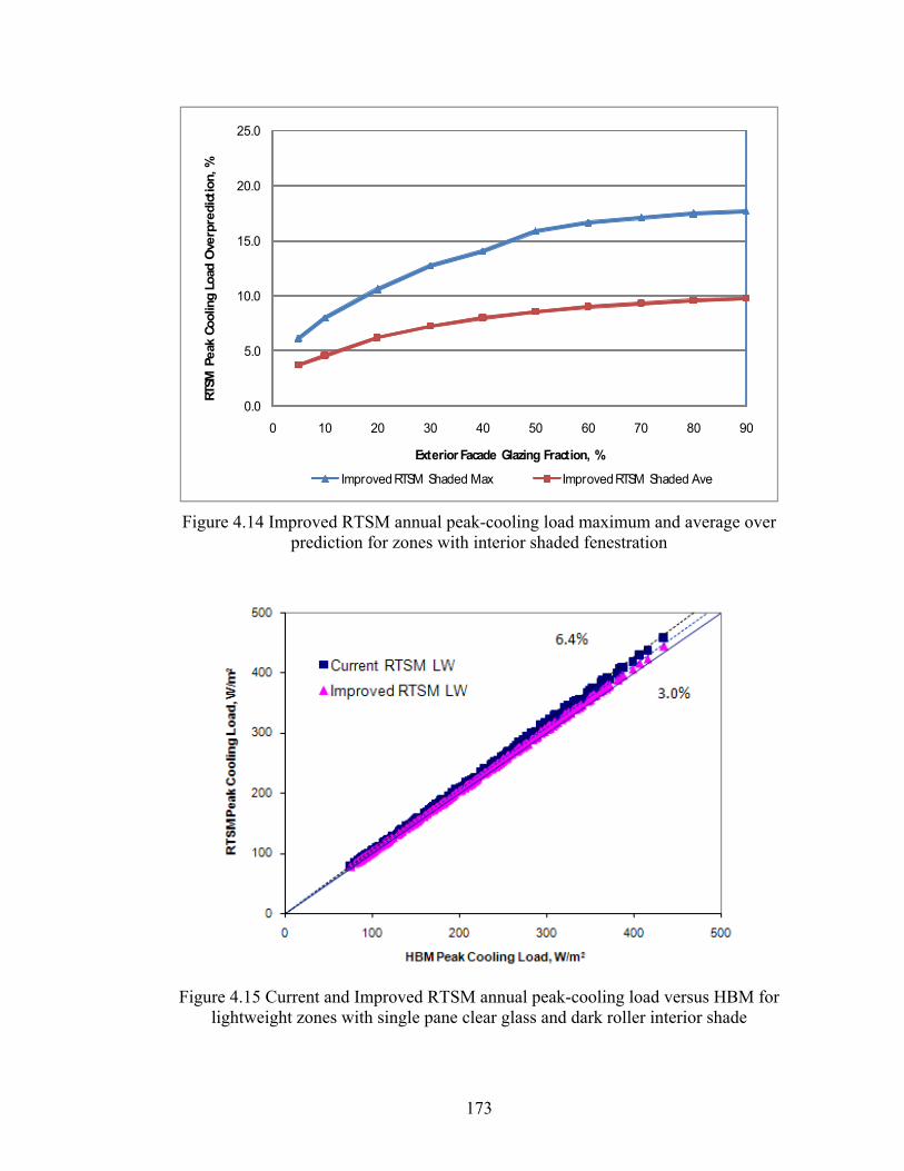
173
0.0
5.0
10.0
15.0
20.0
25.0
0 10 20 30 40 50 60 70 80 90
RTSM
Pea
k Co
olin
g Lo
ad O
verp
redi
ctio
n, %
Exterior Facade Glazing Fraction, %
Improved RTSM Shaded Max Improved RTSM Shaded Ave
Figure 4.14 Improved RTSM annual peak-cooling load maximum and average over prediction for zones with interior shaded fenestration
Figure 4.15 Current and Improved RTSM annual peak-cooling load versus HBM for
lightweight zones with single pane clear glass and dark roller interior shade
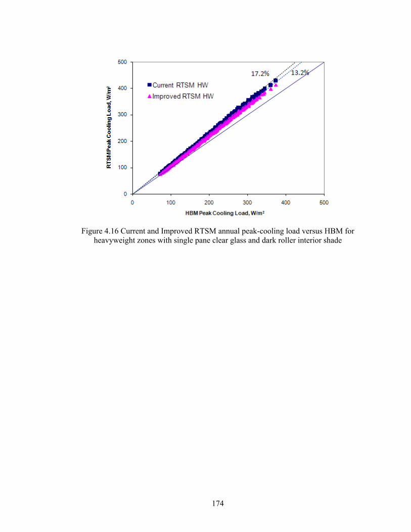
174
Figure 4.16 Current and Improved RTSM annual peak-cooling load versus HBM for
heavyweight zones with single pane clear glass and dark roller interior shade
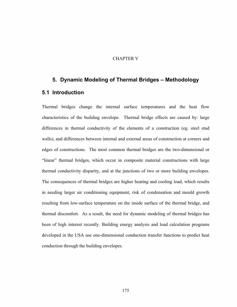
175
CHAPTER V
5. Dynamic Modeling of Thermal Bridges – Methodology
5.1 Introduction Thermal bridges change the internal surface temperatures and the heat flow
characteristics of the building envelope. Thermal bridge effects are caused by: large
differences in thermal conductivity of the elements of a construction (eg. steel stud
walls), and differences between internal and external areas of construction at corners and
edges of constructions. The most common thermal bridges are the two-dimensional or
“linear” thermal bridges, which occur in composite material constructions with large
thermal conductivity disparity, and at the junctions of two or more building envelopes.
The consequences of thermal bridges are higher heating and cooling load, which results
in needing larger air conditioning equipment, risk of condensation and mould growth
resulting from low-surface temperature on the inside surface of the thermal bridge, and
thermal discomfort. As a result, the need for dynamic modeling of thermal bridges has
been of high interest recently. Building energy analysis and load calculation programs
developed in the USA use one-dimensional conduction transfer functions to predict heat
conduction through the building envelopes.
176
In order to properly analyze thermal bridge effect, some form of multi-dimensional
transient heat conduction model is needed. There have been repeated efforts to develop
multidimensional dynamic heat conduction models that produce CTFs in one-
dimensional form for energy analysis and load calculation programs commonly used in
USA. However, their implementation has been delayed for several reasons. A
multidimensional finite volume numerical method has been also implemented in ESP-r
(Nakhi, 1995), which is a whole building energy and environmental simulation program,
but this feature is not usable. Therefore, there is an urgent need for simple one-
dimensional approximate dynamic modeling procedure for constructions with thermal
bridge.
Karambakkam, et al. (2005) proposed a simple one-dimensional approximate procedure
for dynamic modeling of thermal bridges. Preliminary numerical validation results
suggest that this approximate method gives good results from a few cases investigated.
The equivalent homogeneous layer wall model as proposed applies to thermal bridges
with a single composite layer. The procedure does not provide guidance when the
thermal bridge involves multiple composite layers, in particular when two composite
layers are separated by homogeneous layer(s). Furthermore, it does not provide guidance
when to use air-to-air or surface-to-surface R-value. It also does not provide guidance
when a thermal bridge element extends to the surface. This approximate one-dimensional
dynamic model will be investigated experimentally and numerically, and limitations of
this approximate model will be established.
177
5.2 Equivalent Homogeneous Layer Model
The equivalent homogeneous layer (EHL) model (Karambakkam, et al., 2005) is an
approximate one-dimensional dynamic model based on conservation of the thermal
resistance and thermal mass of the actual construction. In this model, an equivalent
homogeneous layer(s) replaces the composite material layer(s). The homogenous layer
resistance is computed such that the actual overall resistance is conserved. The overall
resistance of the actual construction must first be determined using the best method
available. The density and thermal capacity of the equivalent homogeneous layer is
determined based on conservation of thermal mass of the actual construction. The
equivalent homogeneous layer has the following properties:
• Thickness -same as the thickness of composite layer
• Conductivity is determined from the required resistance of the equivalent
homogeneous layer and the thickness of the composite layer
• Density is the volume weighted average of the densities of the composite layer
materials.
• Specific heat is determined from a mass weighted average of the specific heats of
the composite layer materials.
The accuracy of the EHL model in duplicating the actual construction depends on the
accuracy of the steady state thermal resistance or R-value. The equivalent homogeneous
layer produces very good match provided there is accurate knowledge of the overall
thermal resistance or U-value of the actual construction. The following section discusses
ASHRAE’s recommended overall thermal resistance, R-value calculation procedures.
178
5.2.1 Steady State R-Value
Steady state thermal resistances calculation procedures recommended by ASHRAE are
described in Section 2.2.2. Though there are three procedures for overall resistance
calculation recommended by ASHRAE, still there exists some subjective judgment to be
made in selecting the best method for a particular construction type. ASHRAE’s
recommended R-value / U-value calculation procedure are approximations which
sometimes can have significant errors. Therefore, it is worth mentioning that the best R-
value / U-value calculation procedure in accuracy poses limitation on the equivalent
homogeneous layers. However, if accuracy is desired accurate multidimensional
numerical procedures such as finite volume or finite element method can be used to
determine the R-value.
The equivalent homogeneous layer model is believed to give good approximation when a
composite layer or layers of a construction are fully sandwiched between homogeneous
layers. The equivalent homogeneous layer wall model has limitations when the highly
conductive element fully penetrates the outermost layers. The following section the
procedure for computing the equivalent homogeneous layer model is described.
5.2.2 Step By Step Procedure
The equivalent homogeneous layer model (Karambakkam, et al., 2005) relies on accurate
knowledge of the air-to-air or surface-to-surface R-value and the geometry of the actual
construction. The step-by-step procedure for calculating the equivalent homogeneous
layer model wall for cases with single composite layer is described as follows:
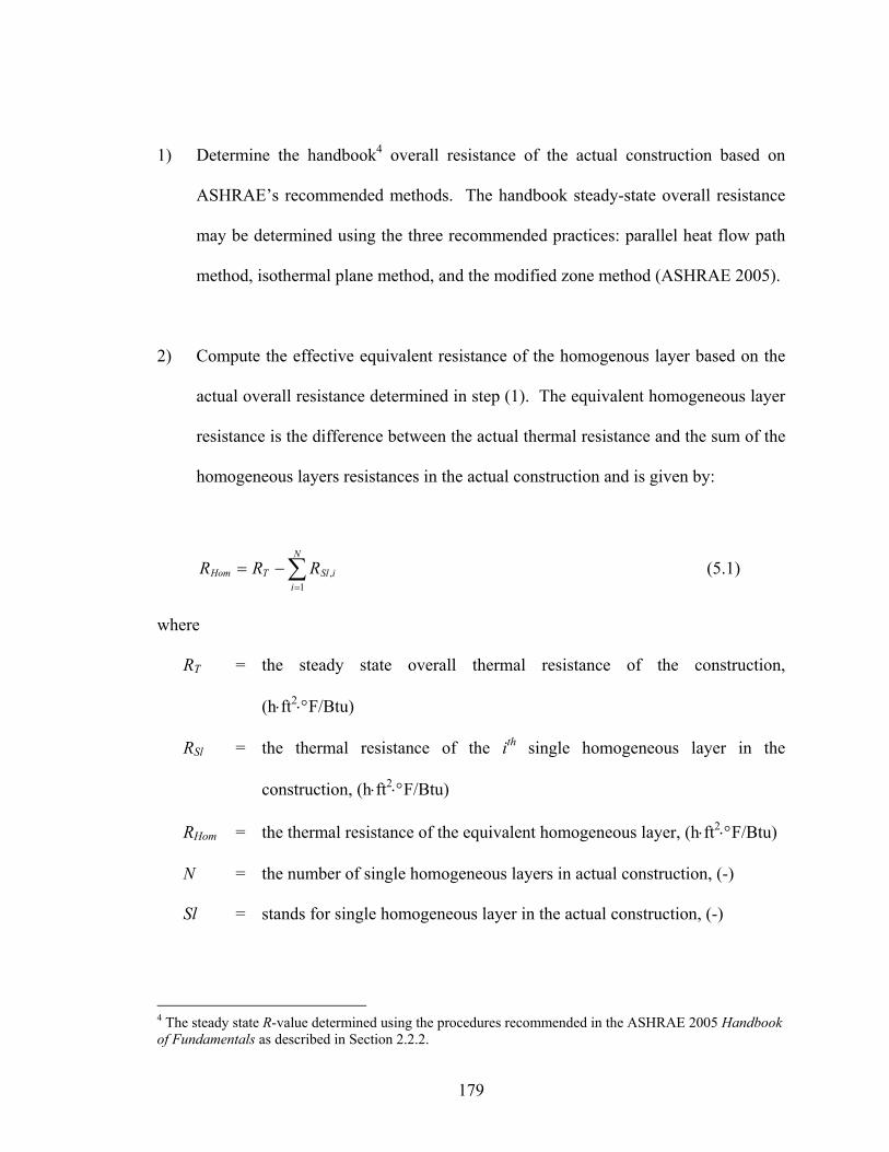
179
1) Determine the handbook4 overall resistance of the actual construction based on
ASHRAE’s recommended methods. The handbook steady-state overall resistance
may be determined using the three recommended practices: parallel heat flow path
method, isothermal plane method, and the modified zone method (ASHRAE 2005).
2) Compute the effective equivalent resistance of the homogenous layer based on the
actual overall resistance determined in step (1). The equivalent homogeneous layer
resistance is the difference between the actual thermal resistance and the sum of the
homogeneous layers resistances in the actual construction and is given by:
∑=
−=N
iiSlTHom RRR
1, (5.1)
where
RT = the steady state overall thermal resistance of the construction,
(h⋅ft2⋅°F/Btu)
RSl = the thermal resistance of the ith single homogeneous layer in the
construction, (h⋅ft2⋅°F/Btu)
RHom = the thermal resistance of the equivalent homogeneous layer, (h⋅ft2⋅°F/Btu)
N = the number of single homogeneous layers in actual construction, (-)
Sl = stands for single homogeneous layer in the actual construction, (-)
4 The steady state R-value determined using the procedures recommended in the ASHRAE 2005 Handbook of Fundamentals as described in Section 2.2.2.
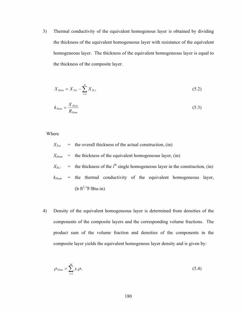
180
3) Thermal conductivity of the equivalent homogenous layer is obtained by dividing
the thickness of the equivalent homogeneous layer with resistance of the equivalent
homogeneous layer. The thickness of the equivalent homogeneous layer is equal to
the thickness of the composite layer.
∑=
−=N
iiSlTotHom XXX
1, (5.2)
Hom
HomHom R
Xk = (5.3)
Where
XTot = the overall thickness of the actual construction, (in)
XHom = the thickness of the equivalent homogeneous layer, (in)
XSl,i = the thickness of the ith single homogeneous layer in the construction, (in)
kHom = the thermal conductivity of the equivalent homogeneous layer,
(h⋅ft2⋅oF/Btu-in)
4) Density of the equivalent homogeneous layer is determined from densities of the
components of the composite layers and the corresponding volume fractions. The
product sum of the volume fraction and densities of the components in the
composite layer yields the equivalent homogenous layer density and is given by:
∑=
=M
iiiHom y
1ρρ (5.4)
181
where
yi = the volume fraction of ith component in the composite layer(s), (-)
ρi = the density of the ith component in the composite layer(s), (lbm/ft3)
ρHom = the density of the equivalent homogeneous layer, (lbm/ft3)
The constituents’ volume fraction in the composite layer is determined from the
geometry of the composite layer.
5) The specific heat of the homogeneous layer is determined from the product sum of
the specific heat, densities and volume fractions of the constituents of the composite
layers.
Hom
M
ipiiiHomP CyC ρρ /
1∑
=
= (5.5)
where
CPi = specific heat of the ith component in the composite layer(s), (Btu/lbm⋅°F)
CP, Hom = specific heat of the equivalent homogeneous layer, (Btu/lbm⋅oF)
Once the thickness and thermo-physical properties of the equivalent homogeneous layer
have been determined, the equivalent homogeneous layers model wall can be input and
analyzed as if were made up of homogeneous layers.

182
The equivalent homogeneous layer wall model described by Karambakkam et al. (2005)
applies to thermal bridges with a single composite layer. It does not provide guidance
when the thermal bridge involves multiple composite layers, in particular when two
composite layers are separated by homogeneous layer(s). It does not provide guidance
whether to use air-to-air or surface-to-surface R-value. It also does not provide guidance
when a thermal bridge element extends to the surface. These practical challenges will be
addressed in Chapter Six and guidance will be developed. Moreover, the equivalent
homogeneous layer model will be validated experimentally, and numerically over a wider
range of construction types.
183
CHAPTER VI
6. Dynamic Modeling of Thermal Bridges – Validation
An approximate one-dimensional homogeneous layer procedure has been proposed for
dynamic modeling of thermal bridges in Chapter 3. The model has been tested
numerically using a few test samples. Preliminary results (Karambakkam et al. 2005)
suggest that the model is promising based on the few limited test cases analyzed.
However, the procedure needs to be tested against a wider range of thermal bridge test
samples to establish its accuracy and limitations. This chapter is dedicated to
experimental and numerical validation of the approximate homogeneous layer one-
dimensional thermal bridge model. The experimental validation of the procedure will be
done utilizing the work of ASHRAE 515-RP (Brown and Stephenson 1993a; Brown and
Stephenson 1993b).
The experimental test data available is limited to seven walls. Therefore, a numerical
experiment that covers a wide range of thermal bridges and boundary conditions is also
proposed. The numerical experiment uses a 2D finite volume method as a reference
model.
184
The following sections describe the experimental validations already done and are
followed by a discussion of the proposed work for the numerical validation. Moreover,
the equivalent homogeneous layer will be extended for use with multiple composite
layers, application and design guidance procedures will be provided for use with real
world thermal bridge types. Besides, guidance will be provided when to use the air-to-air
and the surface to-surface R-value.
6.1 Experimental Validation Experimental validation of the simplified equivalent homogeneous layer (EHL) model is
carried out based on the ASHRAE 515-RP seven experimental test of walls Brown and
Stephenson (1993a; 1993b). The tests were conducted in a dynamic test facility built by
Brown and Stephenson (1993b). The test facility was based on ASTM standard C-236-
89, which applies only to a steady state conditions. The above authors extended the
methodology to make dynamic tests. The experimental validation describes the test
facility and test procedure, the validation and discusses the results.
6.1.1 Guarded Hot Box Dynamic Response Test Facility
The guarded hotbox dynamic response test facility is based on the standard guarded
hotbox steady state test setup with additional control features that dynamically update the
boundary conditions set points Brown and Stephenson (1993b). The experimental set-up
of the guarded hotbox dynamic test facility may be summarized as follows:

185
• Thermally insulated room chamber with a controlled calorimeter. The
calorimeter has a test temperature range 16oC – 26oC and a test area of 2440mm
by 2440mm for full-scale wall specimen test.
• The calorimeter has equally spaced built-in thermocouples measuring the surface
temperatures on both sides of the calorimeter. This allows the measurement of
average temperature of both surfaces of the calorimeter. The set point
temperatures of the calorimeter surfaces are controlled remotely.
• The specimen surface, which faces the calorimeter, is shielded from direct
radiation coming from the calorimeter by a baffle. The baffle is placed between
the calorimeter and the specimen. The baffle has enough spacing for circulation
of the heated air in the space between the calorimeter and the specimen.
• The calorimeter air heater is placed in between the calorimeter and the baffle.
The calorimeter air temperature is sensed and controlled using an analog millivolt
controller.
• The well-insulated cold chamber minimizes the interaction of the cold side of the
specimen with the surroundings and maintains the cold chamber temperature in
the range 0oC to -40oC. Circulating heated air controls the cold chamber
temperature. A pre-cooler maintains the circulating air temperatures below the set
point.
• The set point temperatures in the calorimeter, room chamber and cold chamber
are controlled using a computerized data acquisition system and a remote
controller. For the dynamic tests the set point temperature in the calorimeter is
updated at the required time interval and the controller regulates the new set point
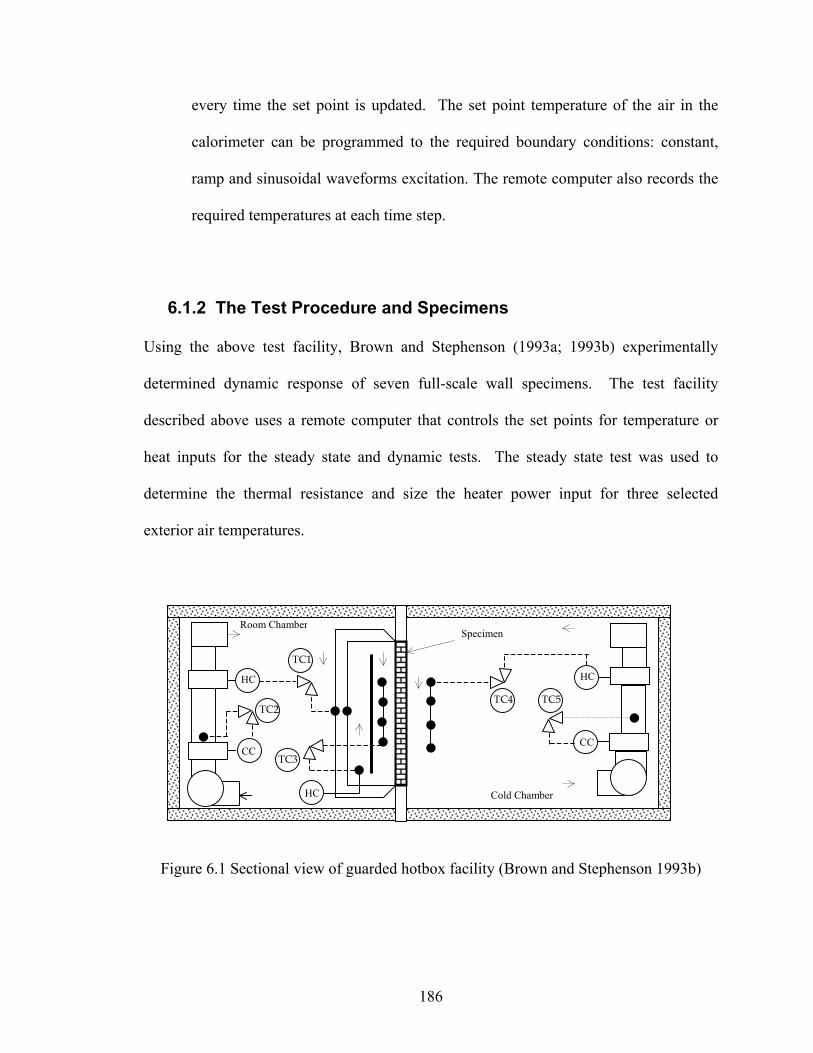
186
every time the set point is updated. The set point temperature of the air in the
calorimeter can be programmed to the required boundary conditions: constant,
ramp and sinusoidal waveforms excitation. The remote computer also records the
required temperatures at each time step.
6.1.2 The Test Procedure and Specimens
Using the above test facility, Brown and Stephenson (1993a; 1993b) experimentally
determined dynamic response of seven full-scale wall specimens. The test facility
described above uses a remote computer that controls the set points for temperature or
heat inputs for the steady state and dynamic tests. The steady state test was used to
determine the thermal resistance and size the heater power input for three selected
exterior air temperatures.
Figure 6.1 Sectional view of guarded hotbox facility (Brown and Stephenson 1993b)
Cold Chamber
SpecimenRoom Chamber
HC
CC
TC1HC
CCTC3
TC4
HC
TC5TC2
187
Legend
HC Heating Coil (Electric Heater)
CC Cooling Coil (Chilled water coiling coil)
TC1 Metering Box differential temperature cooler
TC2 Room air pre-Cooler controller
TC3 Metering box air temperature controller
TC4 Cold Chamber air temperature controller
TC5 Cold Chamber air pre-cooler controller
The mean interior air temperature was fixed at 21°C [70°F] for all the tests. Thermal
resistances of the wall specimens were measured at three different mean exterior air
temperatures: -35°C [-31°F], -20°C [-4°F] and -5°C [23°F]. The thermal resistances
measured for each specimen at these three temperatures were used to establish the
temperature dependent relationship for the thermal resistance.
The dynamic responses of the wall specimens were determined with sinusoidally varying
exterior air temperature at a mean value of -20°C [-4°F] and amplitude of 15K [27°F] at a
period of 24, 12, and 6 hours. For heavy specimens, walls# 2, 3, 4, 5, and 7, a 48 period
was also applied. The calorimeter heat input was fixed at a value determined by steady
state heat transfer rate across the specimen at mean exterior temperature of -20°C [-4°F].
The sinusoidally varying exterior air temperature set point is updated every minute and
the controller of the cold chamber matches the air temperature to the new set point.
188
Another set of dynamic response of the wall specimens was measured for sinusoidal
varying calorimeter heat input with amplitude of 60W at periods of 24, 12, and 6 hours.
For heavy specimens, walls# 2, 3, 4, 5, and 7, a 48 period was also applied. The cold
chamber (exterior air temperature) -35°C [-31°F] fixed air temperature was used. For
this case, the mean calorimeter heater set point was determined from the steady state heat
transfer rate across the specimen measured at a fixed exterior air temperature of -35°C [-
31°F]. The full-scale test specimens are described in Table 6.1.
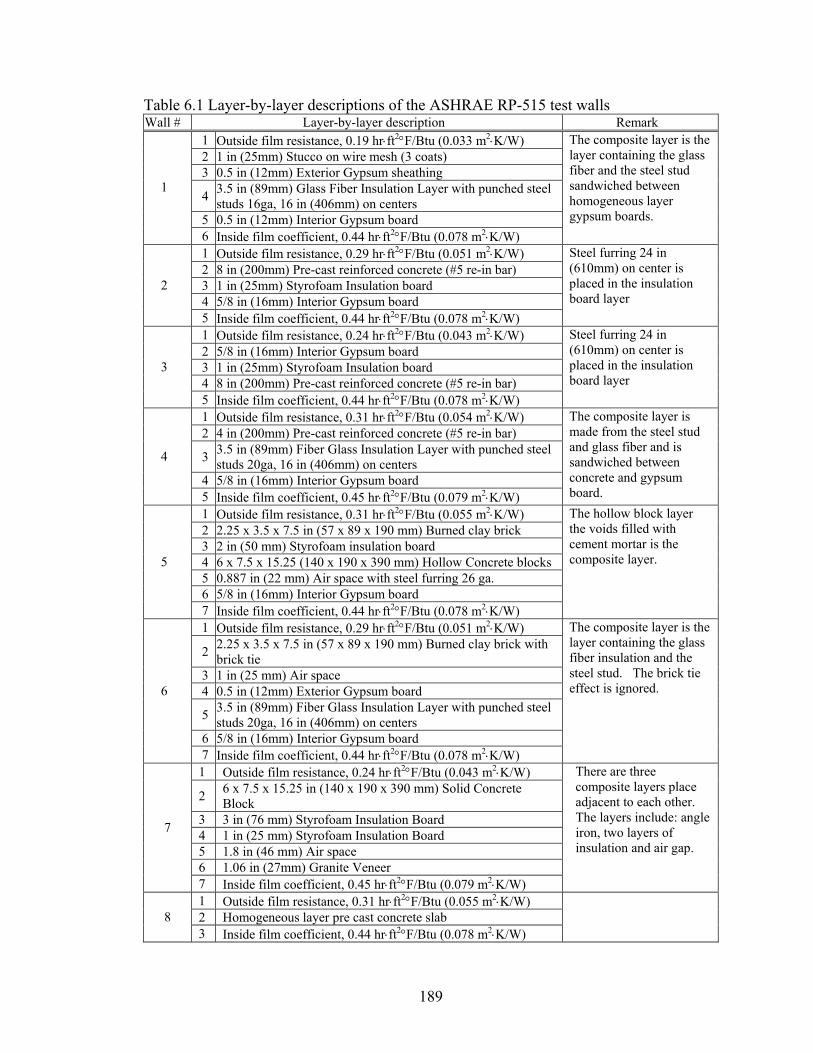
189
Table 6.1 Layer-by-layer descriptions of the ASHRAE RP-515 test walls Wall # Layer-by-layer description Remark
1 Outside film resistance, 0.19 hr⋅ft2°F/Btu (0.033 m2⋅K/W) 2 1 in (25mm) Stucco on wire mesh (3 coats) 3 0.5 in (12mm) Exterior Gypsum sheathing
4 3.5 in (89mm) Glass Fiber Insulation Layer with punched steel studs 16ga, 16 in (406mm) on centers
5 0.5 in (12mm) Interior Gypsum board
1
6 Inside film coefficient, 0.44 hr⋅ft2°F/Btu (0.078 m2⋅K/W)
The composite layer is the layer containing the glass fiber and the steel stud sandwiched between homogeneous layer gypsum boards.
1 Outside film resistance, 0.29 hr⋅ft2°F/Btu (0.051 m2⋅K/W) 2 8 in (200mm) Pre-cast reinforced concrete (#5 re-in bar) 3 1 in (25mm) Styrofoam Insulation board 4 5/8 in (16mm) Interior Gypsum board
2
5 Inside film coefficient, 0.44 hr⋅ft2°F/Btu (0.078 m2⋅K/W)
Steel furring 24 in (610mm) on center is placed in the insulation board layer
1 Outside film resistance, 0.24 hr⋅ft2°F/Btu (0.043 m2⋅K/W) 2 5/8 in (16mm) Interior Gypsum board 3 1 in (25mm) Styrofoam Insulation board 4 8 in (200mm) Pre-cast reinforced concrete (#5 re-in bar)
3
5 Inside film coefficient, 0.44 hr⋅ft2°F/Btu (0.078 m2⋅K/W)
Steel furring 24 in (610mm) on center is placed in the insulation board layer
1 Outside film resistance, 0.31 hr⋅ft2°F/Btu (0.054 m2⋅K/W) 2 4 in (200mm) Pre-cast reinforced concrete (#5 re-in bar)
3 3.5 in (89mm) Fiber Glass Insulation Layer with punched steel studs 20ga, 16 in (406mm) on centers
4 5/8 in (16mm) Interior Gypsum board
4
5 Inside film coefficient, 0.45 hr⋅ft2°F/Btu (0.079 m2⋅K/W)
The composite layer is made from the steel stud and glass fiber and is sandwiched between concrete and gypsum board.
1 Outside film resistance, 0.31 hr⋅ft2°F/Btu (0.055 m2⋅K/W) 2 2.25 x 3.5 x 7.5 in (57 x 89 x 190 mm) Burned clay brick 3 2 in (50 mm) Styrofoam insulation board 4 6 x 7.5 x 15.25 (140 x 190 x 390 mm) Hollow Concrete blocks 5 0.887 in (22 mm) Air space with steel furring 26 ga. 6 5/8 in (16mm) Interior Gypsum board
5
7 Inside film coefficient, 0.44 hr⋅ft2°F/Btu (0.078 m2⋅K/W)
The hollow block layer the voids filled with cement mortar is the composite layer.
1 Outside film resistance, 0.29 hr⋅ft2°F/Btu (0.051 m2⋅K/W)
2 2.25 x 3.5 x 7.5 in (57 x 89 x 190 mm) Burned clay brick with brick tie
3 1 in (25 mm) Air space 4 0.5 in (12mm) Exterior Gypsum board
5 3.5 in (89mm) Fiber Glass Insulation Layer with punched steel studs 20ga, 16 in (406mm) on centers
6 5/8 in (16mm) Interior Gypsum board
6
7 Inside film coefficient, 0.44 hr⋅ft2°F/Btu (0.078 m2⋅K/W)
The composite layer is the layer containing the glass fiber insulation and the steel stud. The brick tie effect is ignored.
1 Outside film resistance, 0.24 hr⋅ft2°F/Btu (0.043 m2⋅K/W)
2 6 x 7.5 x 15.25 in (140 x 190 x 390 mm) Solid Concrete Block
3 3 in (76 mm) Styrofoam Insulation Board 4 1 in (25 mm) Styrofoam Insulation Board 5 1.8 in (46 mm) Air space 6 1.06 in (27mm) Granite Veneer
7
7 Inside film coefficient, 0.45 hr⋅ft2°F/Btu (0.079 m2⋅K/W)
There are three composite layers place adjacent to each other. The layers include: angle iron, two layers of insulation and air gap.
1 Outside film resistance, 0.31 hr⋅ft2°F/Btu (0.055 m2⋅K/W) 2 Homogeneous layer pre cast concrete slab 8 3 Inside film coefficient, 0.44 hr⋅ft2°F/Btu (0.078 m2⋅K/W)
190
6.1.3 Experimental Determination of the CTF
The conduction transfer functions for the test specimens were determined from measured
heat fluxes and/or power inputs, measured temperatures and temperature excitations,
measured U-values and test apparatus calibrations. The z-transfer function coefficients
are determined from the measured responses and U-values using mathematical
manipulations. The following section describes the fundamentals of conduction transfer
functions, describes the procedures for determining the responses, and then describes the
step-by-step procedure for computing the z-transfer coefficients from the measured
responses.
The Laplace transform form of the overall transmission matrix of a multi-layered wall
that relates the transform of the interior temperature Ti, exterior temperature Te, the inside
surface heat flux qi, and the exterior surface heat flux qe and is given by Carslaw and
Jaeger (1959):
⋅
=
e
e
i
i
qT
DCBA
qT
(6.1)
The transmission matrix elements A, B, C and D are functions of the thermal properties
and dimensions of the individual wall layers and the surface heat transfer coefficients.
The matrix element C can be eliminated using the identity AD-BC = 1 and the equation
4.1 can be written as follows:
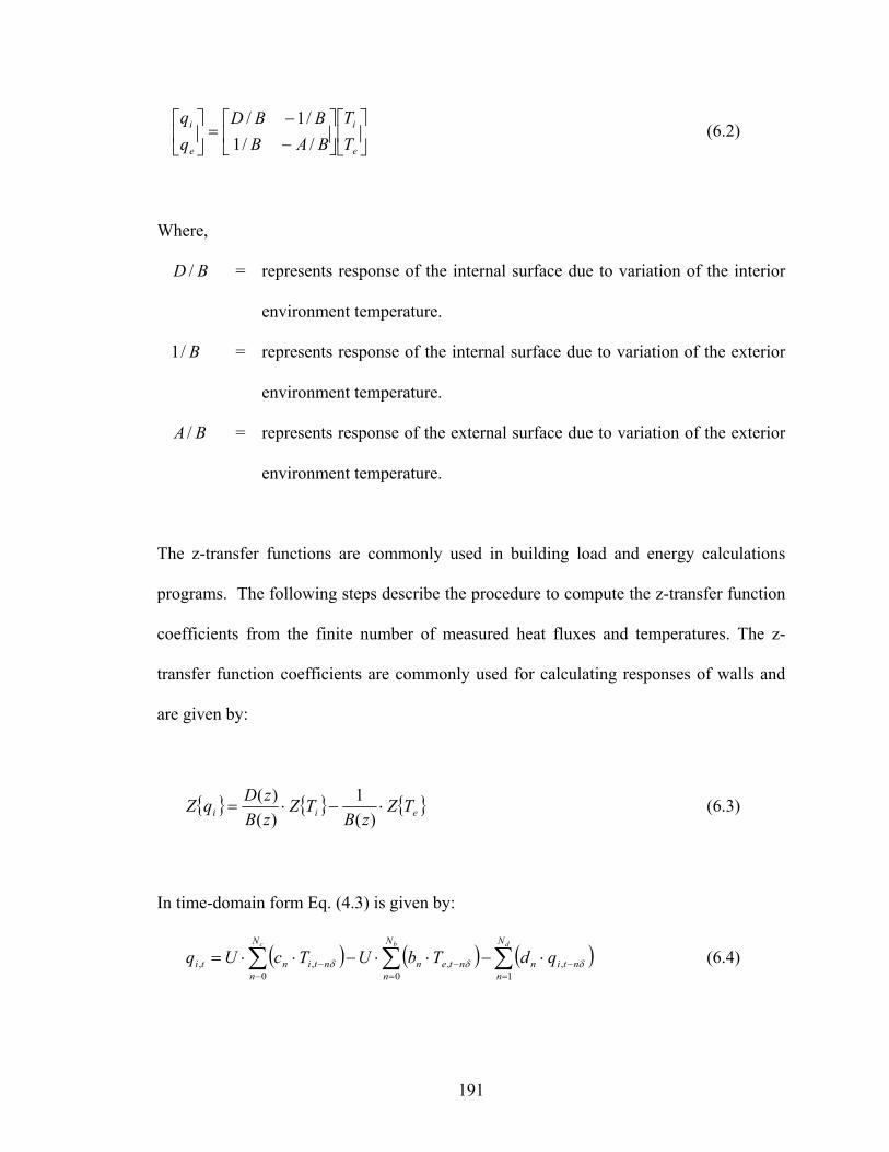
191
−−
=
e
i
e
i
TT
BABBBD
//1/1/
(6.2)
Where,
BD / = represents response of the internal surface due to variation of the interior
environment temperature.
B/1 = represents response of the internal surface due to variation of the exterior
environment temperature.
BA / = represents response of the external surface due to variation of the exterior
environment temperature.
The z-transfer functions are commonly used in building load and energy calculations
programs. The following steps describe the procedure to compute the z-transfer function
coefficients from the finite number of measured heat fluxes and temperatures. The z-
transfer function coefficients are commonly used for calculating responses of walls and
are given by:
eii TZzB
TZzBzDqZ ⋅−⋅=
)(1
)()( (6.3)
In time-domain form Eq. (4.3) is given by:
( ) ( ) ( )∑∑∑=
−=
−−
− ⋅−⋅⋅−⋅⋅=dbc N
nntin
N
nnten
N
nntinti qdTbUTcUq
1,
0,
0,, δδδ (6.4)
192
where,
U = is the air-to-air heat transfer coefficient, W/(m2⋅K)
c = are the inside z-transfer function coefficients, W/(m2⋅ K)
b = are the cross z-transfer function coefficients, W/(m2⋅ K)
d = are heat flux history terms coefficients, (-)
Determination of Wall Response
The cross and inside self-response and time constants of the test walls specimens were
determined as follows (Brown and Stephenson 1993a; 1993b):
1. The values of “D/B”, the inside self-response, were determined from measured heat
flux through the room side (interior) of the specimen in response to an excitation on
the room side of the specimen, and from the test apparatus dynamic calibration.
2. The values of “1/B”, the cross response, were determined from measured heat flux
through the room side (interior) of the specimen in response to an excitation on the
outside of the specimen, and from the test apparatus calibration.
3. A finite number of time constants were determined from the experimental results that
best match the response calculated with Eq. 6.5 to the measured value of 1/B using a
minimization technique at discrete periods.
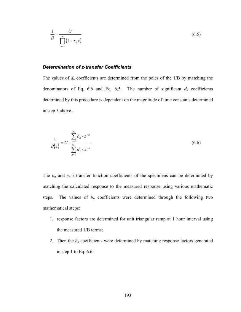
193
( )∏∞
=
+=
1
1
1
nn s
UB τ
(6.5)
Determination of z-transfer Coefficients
The values of dn coefficients are determined from the poles of the 1/B by matching the
denominators of Eq. 6.6 and Eq. 6.5. The number of significant dn coefficients
determined by this procedure is dependent on the magnitude of time constants determined
in step 3 above.
nN
nn
nN
nn
zd
zbU
zB d
b
−
=
−
=
⋅
⋅⋅=
∑
∑
0
01 (6.6)
The bn and cn z-transfer function coefficients of the specimens can be determined by
matching the calculated response to the measured response using various mathematic
steps. The values of bn coefficients were determined through the following two
mathematical steps:
1. response factors are determined for unit triangular ramp at 1 hour interval using
the measured 1/B terms;
2. Then the bn coefficients were determined by matching response factors generated
in step 1 to Eq. 6.6.
194
The values of “cn” are determined by fitting Eq. 6.7 to the frequency response measured
at two periods, typically 24 h and 6h.
n
N
nn
nN
nn
zd
zcU
zBzD
d
c
−
=
−
=
⋅
⋅⋅=
∑
∑
0
0 (6.7)
The test results include the overall and surface-to-surface resistances, the air-to-air z-
transfer functions, and amplitude and phase shift at different periods.
6.1.4 The Experimental Validation Procedure
The equivalent homogeneous layer wall model experimental validation process involves
comparison of the Conduction Time Series Factors (CTSF) coefficients, peak heat gain,
and the peak heat gain timing. For the experimental results, CTSF coefficients are
generated from the CTF coefficients computed by Brown and Stephenson (1993a;
1993b), using the procedure described by Spitler and Fisher (1999a). Using the
experimentally determined surface-to-surface R-value and the construction description
provided by Brown and Stephenson (1993a), the equivalent homogeneous layer model is
used to create an equivalent one-dimensional wall description and Seem’s (1987)
procedure is used to determine CTF coefficients. From these CTFs, the Spitler and
Fisher (1999a) procedure is used to determine CTSF. The two sets of CTSF may be
compared directly.
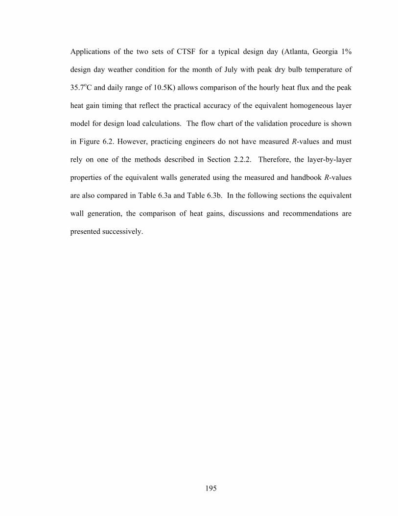
195
Applications of the two sets of CTSF for a typical design day (Atlanta, Georgia 1%
design day weather condition for the month of July with peak dry bulb temperature of
35.7oC and daily range of 10.5K) allows comparison of the hourly heat flux and the peak
heat gain timing that reflect the practical accuracy of the equivalent homogeneous layer
model for design load calculations. The flow chart of the validation procedure is shown
in Figure 6.2. However, practicing engineers do not have measured R-values and must
rely on one of the methods described in Section 2.2.2. Therefore, the layer-by-layer
properties of the equivalent walls generated using the measured and handbook R-values
are also compared in Table 6.3a and Table 6.3b. In the following sections the equivalent
wall generation, the comparison of heat gains, discussions and recommendations are
presented successively.
196
Actual Wall ConstructionData
Experimental Method: • Guarded hotbox dynamic
response test • Sinusoidal varying
temperature boundary condition
• Sinusoidal varying heat flux boundary condition
• Steady state boundary condition
Equivalent Wall Generation: • Using Measured R • Using Calculated R
Air-to-air CTF R-value Amplitude and Phase Shift
Generate: Air-to-air CTSF from CTF
Generate: Air-to-air CTSF with measured RAir-to-air CTSF with calculated R
Comparison: • CTSF • Peak heat gain • Peak heat gain time
Figure 6.2 Flow chart of the experimental validation procedure
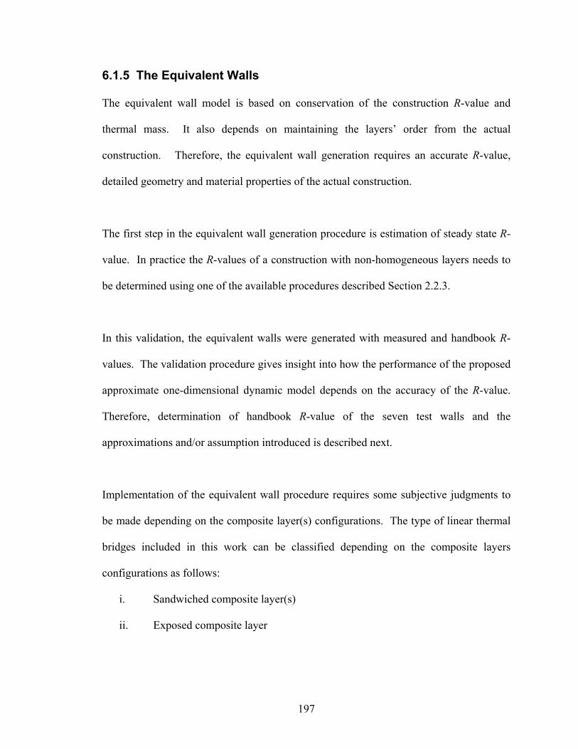
197
6.1.5 The Equivalent Walls
The equivalent wall model is based on conservation of the construction R-value and
thermal mass. It also depends on maintaining the layers’ order from the actual
construction. Therefore, the equivalent wall generation requires an accurate R-value,
detailed geometry and material properties of the actual construction.
The first step in the equivalent wall generation procedure is estimation of steady state R-
value. In practice the R-values of a construction with non-homogeneous layers needs to
be determined using one of the available procedures described Section 2.2.3.
In this validation, the equivalent walls were generated with measured and handbook R-
values. The validation procedure gives insight into how the performance of the proposed
approximate one-dimensional dynamic model depends on the accuracy of the R-value.
Therefore, determination of handbook R-value of the seven test walls and the
approximations and/or assumption introduced is described next.
Implementation of the equivalent wall procedure requires some subjective judgments to
be made depending on the composite layer(s) configurations. The type of linear thermal
bridges included in this work can be classified depending on the composite layers
configurations as follows:
i. Sandwiched composite layer(s)
ii. Exposed composite layer
198
The thermal bridges analyzed here are the linear type with equal inside and outside
surface areas. (They are not associated with corners).
Sandwich Composite Layers
Constructions with sandwich type composite layers are common in building wall and roof
constructions. The construction may contain one or more composite layer(s) located in
adjacent each other or separated by homogeneous layer(s). This type of thermal bridges
will have at least three layers – two homogeneous layers and one composite layer. They
can be easily replicated easily using the equivalent homogeneous layer wall model. A
typical sandwich type thermal bridge is found in a steel stud walls with siding on exterior
side and dry wall on the interior side as shown in Figure 6.3(a).
(a) (b)
Figure 6.3 Thermal bridge types: (a) sandwiched type; (b) exposed type
Exposed Composite Layer
Thermal bridges involving composite layer(s) exposed to either exterior or interior
environments are not common in building constructions. This type of thermal bridge
cannot be easily replicated by the equivalent homogeneous layer wall model procedure
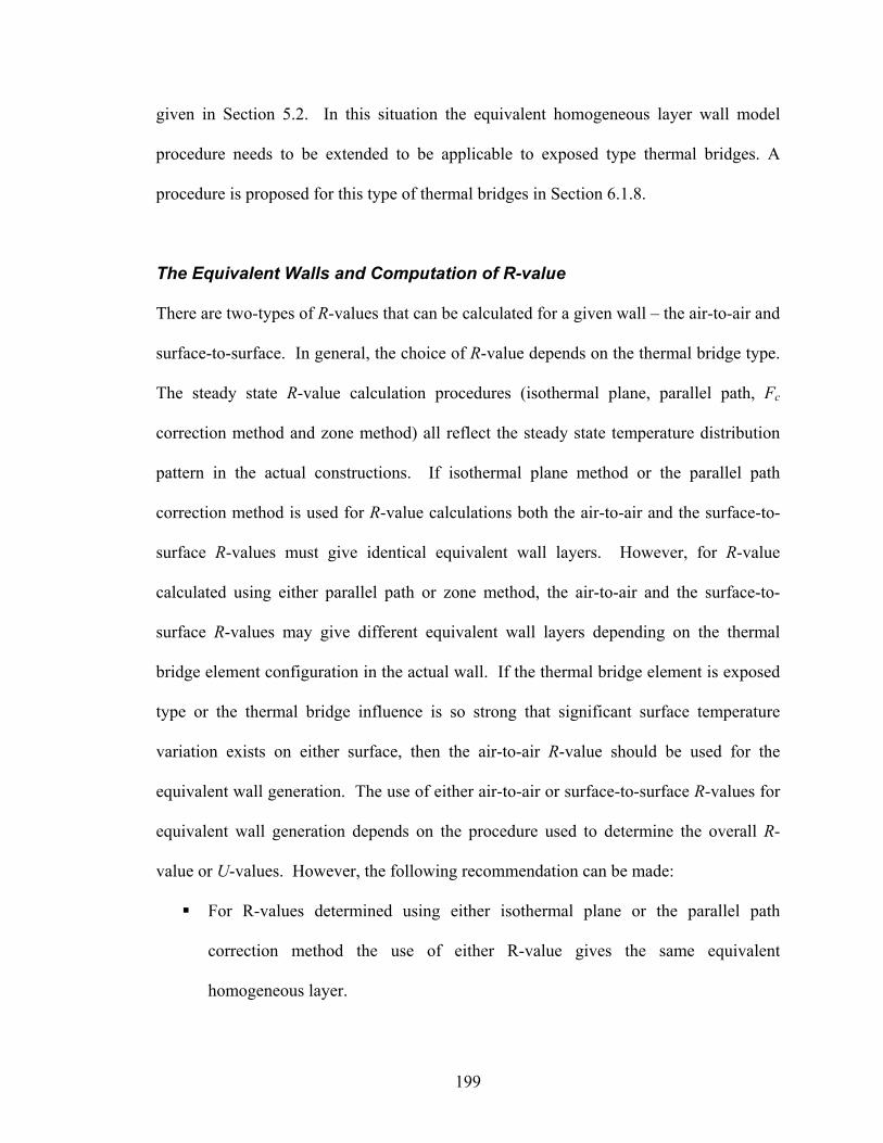
199
given in Section 5.2. In this situation the equivalent homogeneous layer wall model
procedure needs to be extended to be applicable to exposed type thermal bridges. A
procedure is proposed for this type of thermal bridges in Section 6.1.8.
The Equivalent Walls and Computation of R-value
There are two-types of R-values that can be calculated for a given wall – the air-to-air and
surface-to-surface. In general, the choice of R-value depends on the thermal bridge type.
The steady state R-value calculation procedures (isothermal plane, parallel path, Fc
correction method and zone method) all reflect the steady state temperature distribution
pattern in the actual constructions. If isothermal plane method or the parallel path
correction method is used for R-value calculations both the air-to-air and the surface-to-
surface R-values must give identical equivalent wall layers. However, for R-value
calculated using either parallel path or zone method, the air-to-air and the surface-to-
surface R-values may give different equivalent wall layers depending on the thermal
bridge element configuration in the actual wall. If the thermal bridge element is exposed
type or the thermal bridge influence is so strong that significant surface temperature
variation exists on either surface, then the air-to-air R-value should be used for the
equivalent wall generation. The use of either air-to-air or surface-to-surface R-values for
equivalent wall generation depends on the procedure used to determine the overall R-
value or U-values. However, the following recommendation can be made:
For R-values determined using either isothermal plane or the parallel path
correction method the use of either R-value gives the same equivalent
homogeneous layer.
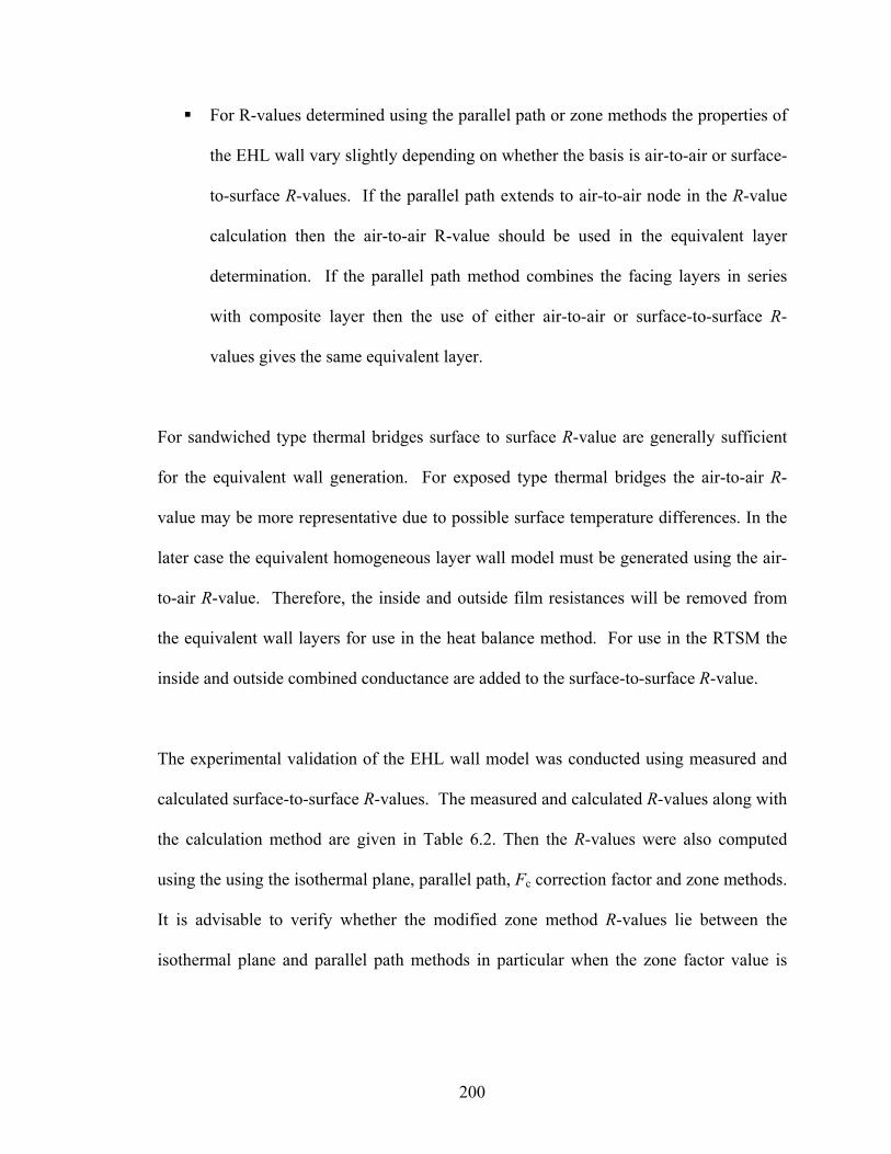
200
For R-values determined using the parallel path or zone methods the properties of
the EHL wall vary slightly depending on whether the basis is air-to-air or surface-
to-surface R-values. If the parallel path extends to air-to-air node in the R-value
calculation then the air-to-air R-value should be used in the equivalent layer
determination. If the parallel path method combines the facing layers in series
with composite layer then the use of either air-to-air or surface-to-surface R-
values gives the same equivalent layer.
For sandwiched type thermal bridges surface to surface R-value are generally sufficient
for the equivalent wall generation. For exposed type thermal bridges the air-to-air R-
value may be more representative due to possible surface temperature differences. In the
later case the equivalent homogeneous layer wall model must be generated using the air-
to-air R-value. Therefore, the inside and outside film resistances will be removed from
the equivalent wall layers for use in the heat balance method. For use in the RTSM the
inside and outside combined conductance are added to the surface-to-surface R-value.
The experimental validation of the EHL wall model was conducted using measured and
calculated surface-to-surface R-values. The measured and calculated R-values along with
the calculation method are given in Table 6.2. Then the R-values were also computed
using the using the isothermal plane, parallel path, Fc correction factor and zone methods.
It is advisable to verify whether the modified zone method R-values lie between the
isothermal plane and parallel path methods in particular when the zone factor value is

201
outside the range for which the method is recommended. The section views of the seven
test walls are shown in Figure 6.4.
The equivalent homogeneous layers are generated using the procedure described in
Chapter 5. The following section discusses the assumptions made and approximations
introduced to generate the equivalent homogeneous layer for each of the seven ASHRAE
test walls.
The following general principles for when to ignore distributed elements of a composite
construction have been followed:
Small elements of negligible conductance such as brick ties are neglected
Element aligned parallel to the wall surface, like rebar, for which the thermal
mass is important but the increased conductance in the transverse direction of the
wall is negligible are neglected for resistance calculation; however, they are
included in the layer thermal mass.
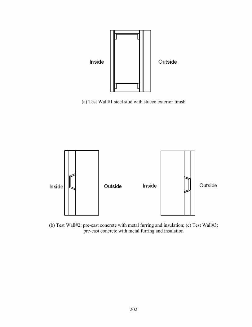
202
(a) Test Wall#1 steel stud with stucco exterior finish
(b) Test Wall#2: pre-cast concrete with metal furring and insulation; (c) Test Wall#3: pre-cast concrete with metal furring and insulation
203
(d) Test Wall#4: Insulated steel stud mounted on pre-cast concrete; (e) Test Wall#5: Hollow Block with insulation and brick exterior finish
(f) Test Wall#6: Insulated steel stud wall with brick finish; (g) Test Wall#7: Solid Concrete block with insulation and granite finish
Figure 6.4 ASHRAE RP-515 Test Walls
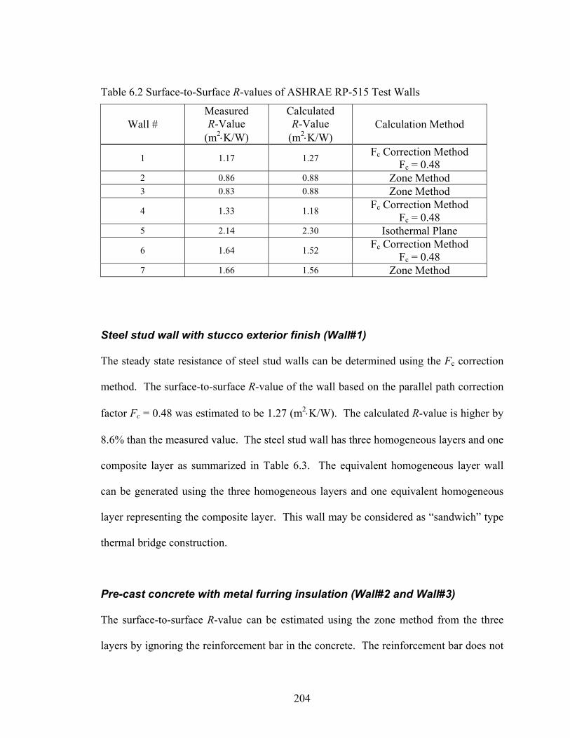
204
Table 6.2 Surface-to-Surface R-values of ASHRAE RP-515 Test Walls
Wall # Measured R-Value
(m2⋅K/W)
Calculated R-Value
(m2⋅K/W) Calculation Method
1 1.17 1.27 Fc Correction Method Fc = 0.48
2 0.86 0.88 Zone Method 3 0.83 0.88 Zone Method
4 1.33 1.18 Fc Correction Method Fc = 0.48
5 2.14 2.30 Isothermal Plane
6 1.64 1.52 Fc Correction Method Fc = 0.48
7 1.66 1.56 Zone Method
Steel stud wall with stucco exterior finish (Wall#1)
The steady state resistance of steel stud walls can be determined using the Fc correction
method. The surface-to-surface R-value of the wall based on the parallel path correction
factor Fc = 0.48 was estimated to be 1.27 (m2⋅K/W). The calculated R-value is higher by
8.6% than the measured value. The steel stud wall has three homogeneous layers and one
composite layer as summarized in Table 6.3. The equivalent homogeneous layer wall
can be generated using the three homogeneous layers and one equivalent homogeneous
layer representing the composite layer. This wall may be considered as “sandwich” type
thermal bridge construction.
Pre-cast concrete with metal furring insulation (Wall#2 and Wall#3)
The surface-to-surface R-value can be estimated using the zone method from the three
layers by ignoring the reinforcement bar in the concrete. The reinforcement bar does not
205
act as thermal bridge element since it is parallel to the inside and outside surface areas
and hence has negligible effect on the thermal resistance. The R-value determined using
the zone method is given in Table 6.3. Test specimen wall#3 is the same construction but
the layers are in reverse order. Therefore both walls should have the same steady state
thermal resistance or R-value. However, the slight difference in experimental
measurement due to instrumentation error or change in the property of the test specimen
may cause difference in the R-values.
These wall constructions each have two homogeneous layers and one composite layer.
The composite layer is made from Styrofoam insulation board and steel furring. An
equivalent homogeneous layer that replaces the composite layer was determined. The
metal reinforcement bars (rebar) in the concrete slabs are accounted for in thermal mass
calculations. This wall may be considered as “sandwich” type thermal bridge
construction.
Insulated steel stud mounted on pre-cast concrete (Wall#4)
The surface-to-surface R-value of the insulation is determined using the
insulation/framing adjustment factor in ASHRAE/IESNA Standard 90.1-2004, in Table
A9.2B Fc=0.48. The handbook R-value (1.18 m2⋅K/W) is lower than the measured value
(1.33 m2⋅K/W) by 11.3% as shown in Table 6.2. Ignoring the metal reinforcement bars in
the concrete slab, the insulated steel stud wall can be considered a “sandwich” type
thermal bridge construction. The glass fiber and the steel stud constitute a composite
206
layer hence can be replaced by an equivalent homogeneous layer. The equivalent wall
consists of three homogeneous layers as summarized in Table 6.3.
Hollow Block with insulation and brick exterior finish (Wall#5)
The surface-to-surface R-value was determined by applying the isothermal plane method
for the hollow block layer. The estimated R-value (2.30 m2⋅K/W) is lower than the
measured R-value (2.14 m2⋅K/W) by 7.5%. All layers except the hollow block section
may be considered as homogeneous layers. The hollow block voids are filled with
cement mortar and hence are considered as composite layers. Thus, an equivalent
homogeneous layer was generated for the hollow block section of the wall. The brick’s
thermal mass was corrected for the voids. All in all the equivalent homogeneous layers
wall contain five homogeneous layers as summarized in Table 6.3. The voids in the brick
are a small fraction of the heat flow path area and the thermal conductivity of the brick
material is significantly higher than the void conductance. Therefore, ignoring the void
resistance has little effect on the overall thermal resistance of the construction.
Insulated steel stud wall with brick finish (Wall#6)
The surface-to-surface R-value was estimated with Fc correction method. The estimated
R-value (1.52 m2⋅K/W) is lower than the measured R-value (1.64 m2⋅K/W) by 7.3%. The
brick ties were ignored in steady state thermal resistance calculations. The steel stud wall
with air space and brick veneer finish can be considered to have only one composite layer
section if the brick ties are ignored. This wall is a sandwich type thermal bridge. The
equivalent homogeneous layer for the composite can be determined using the procedure

207
described in Chapter 5 and the resulting equivalent wall has five homogeneous layers as
shown in Table 6.3.
Solid Concrete block with insulation and granite finish (Wall#7)
This wall consists of a homogeneous layer solid concrete block to which an angle iron is
mounted with bolted connection to support insulation layers. The angle iron extends
through the insulation layers and supports the Veri-trust channel. The wall has an air gap
and a granite veneer exterior finish. The granite veneer is secured by galvanized steel
butterfly clip that extends through the air gap and screwed to the Veri-trust channel as
shown in Figure 6.4g. The insulation and the angle iron form composite layer, the air gap
and Veri-trust channel for the second composite layer and the granite veneer and the
butterfly clip can be considered as the third composite layer. The solid concrete block
could also be considered as the fourth composite layer due to the anchoring bolt.
The surface-to-surface R-value was estimated using the zone method for the composite
layer containing the insulation and angle iron. The width of the thermal bridge metal
section is assumed to be half of that of the angle iron width. The Veri-trust channel was
ignored, as it is aligned perpendicular to the main heat flow path. The butterfly clip has
been also ignored due to small heat flow paths area compared to total surface area. The
estimated R-value (1.77 m2⋅K/W) is higher than the measured R-value (1.69 m2⋅K/W) by
4.7%.
208
All the composite layers are adjacent to each other. The composite layers containing the
two insulation layers and the air gap can be lumped together to form an equivalent
homogeneous layer. Therefore, the equivalent homogeneous layer wall will be formed
from the solid concrete block, the equivalent homogeneous layer and the granite veneer.
The effect of the Veri-trust channel on the thermal mass is included. For the seven walls,
the various ASHRAE methods for predicting steady-state resistances predict the R-values
within ±11.3%. In general, the equivalent homogeneous layer model may be expected to
be no more accurate than the estimate of steady state resistance. The experimental
validation results given in Section 6.1.4 reflect the importance of the R-value on the
accuracy of the proposed model.
The R-value calculation methods and approximations introduced in the equivalent wall
generation for the test walls have been previously discussed. The layer-by-layer
description of the equivalents walls determined using the measured and handbook R-
values are given in Table 6.3a and Table 6.3b, respectively. The difference between the
two equivalent walls generated using the measured and handbook R-values is the
composite layer (equivalent homogeneous layer) thermal resistance; otherwise the
number of layers, layers order, and thermal mass of the construction are the same. The
following sections discuss the effects of R-values have on the equivalent wall CTSFs.
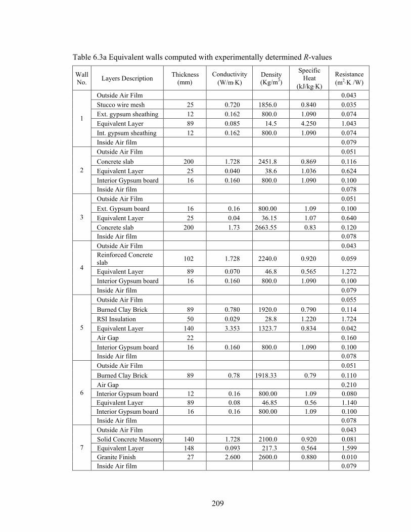
209
Table 6.3a Equivalent walls computed with experimentally determined R-values
Wall No. Layers Description Thickness
(mm) Conductivity
(W/m⋅K) Density (Kg/m3)
Specific Heat
(kJ/kg⋅K)
Resistance (m2⋅K /W)
Outside Air Film 0.043 Stucco wire mesh 25 0.720 1856.0 0.840 0.035 Ext. gypsum sheathing 12 0.162 800.0 1.090 0.074 Equivalent Layer 89 0.085 14.5 4.250 1.043 Int. gypsum sheathing 12 0.162 800.0 1.090 0.074
1
Inside Air film 0.079 Outside Air Film 0.051 Concrete slab 200 1.728 2451.8 0.869 0.116 Equivalent Layer 25 0.040 38.6 1.036 0.624 Interior Gypsum board 16 0.160 800.0 1.090 0.100
2
Inside Air film 0.078 Outside Air Film 0.051 Ext. Gypsum board 16 0.16 800.00 1.09 0.100 Equivalent Layer 25 0.04 36.15 1.07 0.640 Concrete slab 200 1.73 2663.55 0.83 0.120
3
Inside Air film 0.078 Outside Air Film 0.043 Reinforced Concrete slab 102 1.728 2240.0 0.920 0.059
Equivalent Layer 89 0.070 46.8 0.565 1.272 Interior Gypsum board 16 0.160 800.0 1.090 0.100
4
Inside Air film 0.079 Outside Air Film 0.055 Burned Clay Brick 89 0.780 1920.0 0.790 0.114 RSI Insulation 50 0.029 28.8 1.220 1.724 Equivalent Layer 140 3.353 1323.7 0.834 0.042 Air Gap 22 0.160 Interior Gypsum board 16 0.160 800.0 1.090 0.100
5
Inside Air film 0.078 Outside Air Film 0.051 Burned Clay Brick 89 0.78 1918.33 0.79 0.110 Air Gap 0.210 Interior Gypsum board 12 0.16 800.00 1.09 0.080 Equivalent Layer 89 0.08 46.85 0.56 1.140 Interior Gypsum board 16 0.16 800.00 1.09 0.100
6
Inside Air film 0.078 Outside Air Film 0.043 Solid Concrete Masonry 140 1.728 2100.0 0.920 0.081 Equivalent Layer 148 0.093 217.3 0.564 1.599 Granite Finish 27 2.600 2600.0 0.880 0.010
7
Inside Air film 0.079
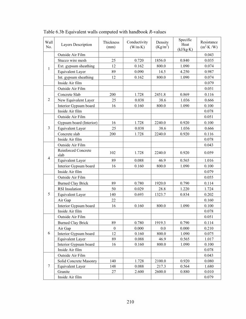
210
Table 6.3b Equivalent walls computed with handbook R-values
Wall No. Layers Description Thickness
(mm) Conductivity
(W/m⋅K) Density (Kg/m3)
Specific Heat
(kJ/kg⋅K)
Resistance (m2⋅K /W)
Outside Air Film 0.043 Stucco wire mesh 25 0.720 1856.0 0.840 0.035 Ext. gypsum sheathing 12 0.162 800.0 1.090 0.074 Equivalent Layer 89 0.090 14.5 4.250 0.987 Int. gypsum sheathing 12 0.162 800.0 1.090 0.074
1
Inside Air film 0.079 Outside Air Film 0.051 Concrete Slab 200 1.728 2451.8 0.869 0.116 New Equivalent Layer 25 0.038 38.6 1.036 0.666 Interior Gypsum board 16 0.160 800.0 1.090 0.100
2
Inside Air film 0.078 Outside Air Film 0.051 Gypsum board (Interior) 16 1.728 2240.0 0.920 0.100 Equivalent Layer 25 0.038 38.6 1.036 0.666 Concrete slab 200 1.728 2240.0 0.920 0.116
3
Inside Air film 0.078 Outside Air Film 0.043 Reinforced Concrete slab 102 1.728 2240.0 0.920 0.059
Equivalent Layer 89 0.088 46.9 0.565 1.016 Interior Gypsum board 16 0.160 800.0 1.090 0.100
4
Inside Air film 0.079 Outside Air Film 0.055 Burned Clay Brick 89 0.780 1920.0 0.790 0.114 RSI Insulation 50 0.029 28.8 1.220 1.724 Equivalent Layer 140 0.693 1323.7 0.834 0.202 Air Gap 22 0.160 Interior Gypsum board 16 0.160 800.0 1.090 0.100
5
Inside Air film 0.078 Outside Air Film 0.051 Burned Clay Brick 89 0.780 1919.3 0.790 0.114 Air Gap 0 0.000 0.0 0.000 0.210 Interior Gypsum board 12 0.160 800.0 1.090 0.075 Equivalent Layer 89 0.088 46.9 0.565 1.017 Interior Gypsum board 16 0.160 800.0 1.090 0.100
6
Inside Air film 0.078 Outside Air Film 0.043 Solid Concrete Masonry 140 1.728 2100.0 0.920 0.080 Equivalent Layer 148 0.088 217.3 0.564 1.680 Granite 27 2.600 2600.0 0.880 0.010
7
Inside Air film 0.079
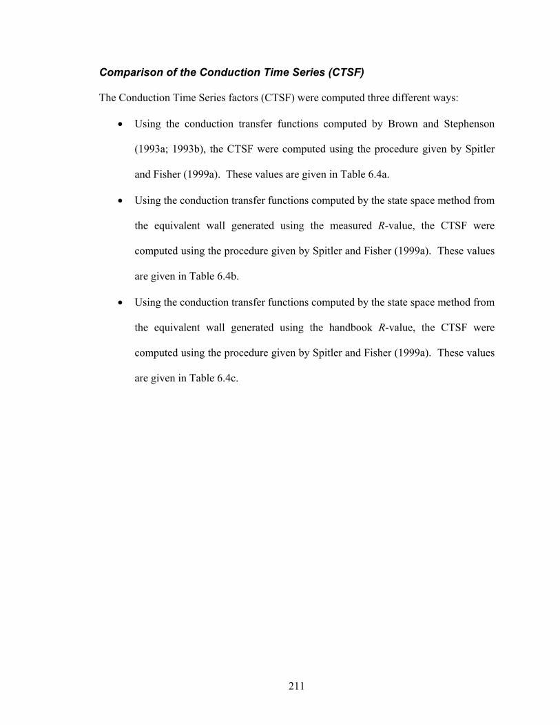
211
Comparison of the Conduction Time Series (CTSF)
The Conduction Time Series factors (CTSF) were computed three different ways:
• Using the conduction transfer functions computed by Brown and Stephenson
(1993a; 1993b), the CTSF were computed using the procedure given by Spitler
and Fisher (1999a). These values are given in Table 6.4a.
• Using the conduction transfer functions computed by the state space method from
the equivalent wall generated using the measured R-value, the CTSF were
computed using the procedure given by Spitler and Fisher (1999a). These values
are given in Table 6.4b.
• Using the conduction transfer functions computed by the state space method from
the equivalent wall generated using the handbook R-value, the CTSF were
computed using the procedure given by Spitler and Fisher (1999a). These values
are given in Table 6.4c.
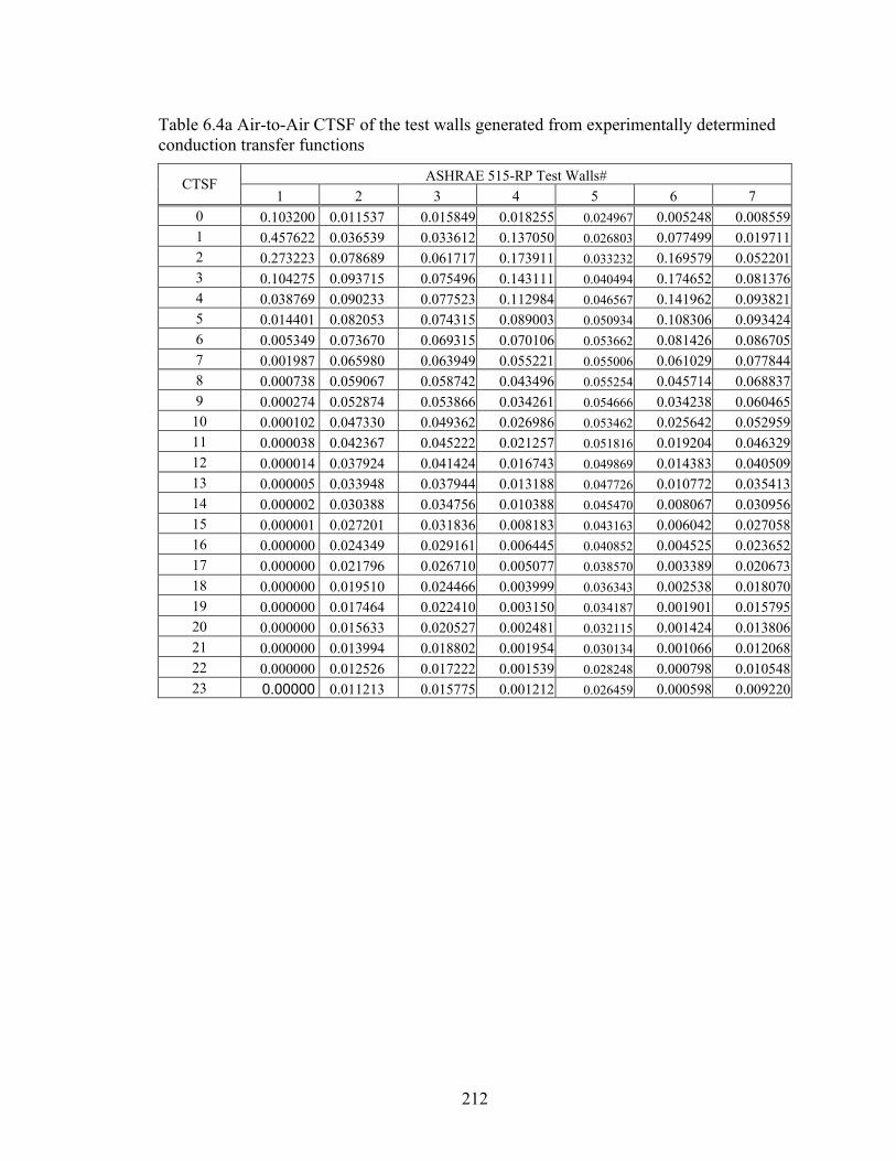
212
Table 6.4a Air-to-Air CTSF of the test walls generated from experimentally determined conduction transfer functions
ASHRAE 515-RP Test Walls# CTSF 1 2 3 4 5 6 7
0 0.103200 0.011537 0.015849 0.018255 0.024967 0.005248 0.0085591 0.457622 0.036539 0.033612 0.137050 0.026803 0.077499 0.0197112 0.273223 0.078689 0.061717 0.173911 0.033232 0.169579 0.0522013 0.104275 0.093715 0.075496 0.143111 0.040494 0.174652 0.0813764 0.038769 0.090233 0.077523 0.112984 0.046567 0.141962 0.0938215 0.014401 0.082053 0.074315 0.089003 0.050934 0.108306 0.0934246 0.005349 0.073670 0.069315 0.070106 0.053662 0.081426 0.0867057 0.001987 0.065980 0.063949 0.055221 0.055006 0.061029 0.0778448 0.000738 0.059067 0.058742 0.043496 0.055254 0.045714 0.0688379 0.000274 0.052874 0.053866 0.034261 0.054666 0.034238 0.060465
10 0.000102 0.047330 0.049362 0.026986 0.053462 0.025642 0.05295911 0.000038 0.042367 0.045222 0.021257 0.051816 0.019204 0.04632912 0.000014 0.037924 0.041424 0.016743 0.049869 0.014383 0.04050913 0.000005 0.033948 0.037944 0.013188 0.047726 0.010772 0.03541314 0.000002 0.030388 0.034756 0.010388 0.045470 0.008067 0.03095615 0.000001 0.027201 0.031836 0.008183 0.043163 0.006042 0.02705816 0.000000 0.024349 0.029161 0.006445 0.040852 0.004525 0.02365217 0.000000 0.021796 0.026710 0.005077 0.038570 0.003389 0.02067318 0.000000 0.019510 0.024466 0.003999 0.036343 0.002538 0.01807019 0.000000 0.017464 0.022410 0.003150 0.034187 0.001901 0.01579520 0.000000 0.015633 0.020527 0.002481 0.032115 0.001424 0.01380621 0.000000 0.013994 0.018802 0.001954 0.030134 0.001066 0.01206822 0.000000 0.012526 0.017222 0.001539 0.028248 0.000798 0.01054823 0.00000 0.011213 0.015775 0.001212 0.026459 0.000598 0.009220
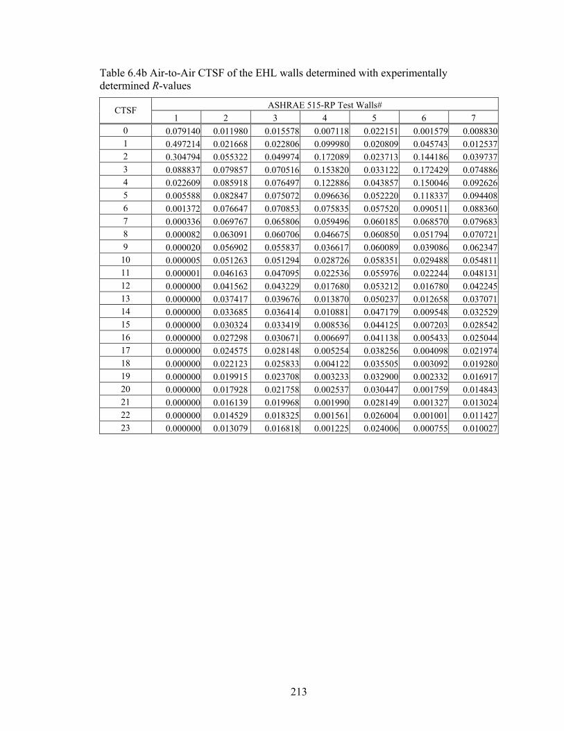
213
Table 6.4b Air-to-Air CTSF of the EHL walls determined with experimentally determined R-values
ASHRAE 515-RP Test Walls# CTSF 1 2 3 4 5 6 7
0 0.079140 0.011980 0.015578 0.007118 0.022151 0.001579 0.0088301 0.497214 0.021668 0.022806 0.099980 0.020809 0.045743 0.0125372 0.304794 0.055322 0.049974 0.172089 0.023713 0.144186 0.0397373 0.088837 0.079857 0.070516 0.153820 0.033122 0.172429 0.0748864 0.022609 0.085918 0.076497 0.122886 0.043857 0.150046 0.0926265 0.005588 0.082847 0.075072 0.096636 0.052220 0.118337 0.0944086 0.001372 0.076647 0.070853 0.075835 0.057520 0.090511 0.0883607 0.000336 0.069767 0.065806 0.059496 0.060185 0.068570 0.0796838 0.000082 0.063091 0.060706 0.046675 0.060850 0.051794 0.0707219 0.000020 0.056902 0.055837 0.036617 0.060089 0.039086 0.062347
10 0.000005 0.051263 0.051294 0.028726 0.058351 0.029488 0.05481111 0.000001 0.046163 0.047095 0.022536 0.055976 0.022244 0.04813112 0.000000 0.041562 0.043229 0.017680 0.053212 0.016780 0.04224513 0.000000 0.037417 0.039676 0.013870 0.050237 0.012658 0.03707114 0.000000 0.033685 0.036414 0.010881 0.047179 0.009548 0.03252915 0.000000 0.030324 0.033419 0.008536 0.044125 0.007203 0.02854216 0.000000 0.027298 0.030671 0.006697 0.041138 0.005433 0.02504417 0.000000 0.024575 0.028148 0.005254 0.038256 0.004098 0.02197418 0.000000 0.022123 0.025833 0.004122 0.035505 0.003092 0.01928019 0.000000 0.019915 0.023708 0.003233 0.032900 0.002332 0.01691720 0.000000 0.017928 0.021758 0.002537 0.030447 0.001759 0.01484321 0.000000 0.016139 0.019968 0.001990 0.028149 0.001327 0.01302422 0.000000 0.014529 0.018325 0.001561 0.026004 0.001001 0.01142723 0.000000 0.013079 0.016818 0.001225 0.024006 0.000755 0.010027
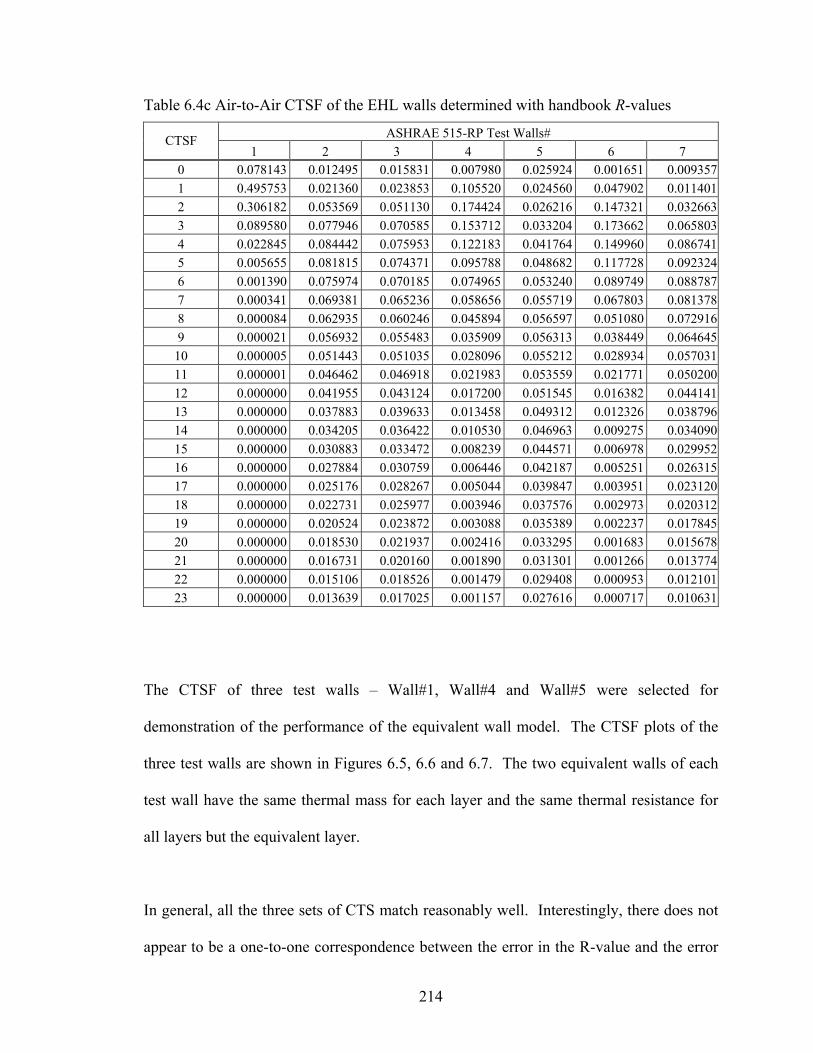
214
Table 6.4c Air-to-Air CTSF of the EHL walls determined with handbook R-values
ASHRAE 515-RP Test Walls# CTSF 1 2 3 4 5 6 7
0 0.078143 0.012495 0.015831 0.007980 0.025924 0.001651 0.0093571 0.495753 0.021360 0.023853 0.105520 0.024560 0.047902 0.0114012 0.306182 0.053569 0.051130 0.174424 0.026216 0.147321 0.0326633 0.089580 0.077946 0.070585 0.153712 0.033204 0.173662 0.0658034 0.022845 0.084442 0.075953 0.122183 0.041764 0.149960 0.0867415 0.005655 0.081815 0.074371 0.095788 0.048682 0.117728 0.0923246 0.001390 0.075974 0.070185 0.074965 0.053240 0.089749 0.0887877 0.000341 0.069381 0.065236 0.058656 0.055719 0.067803 0.0813788 0.000084 0.062935 0.060246 0.045894 0.056597 0.051080 0.0729169 0.000021 0.056932 0.055483 0.035909 0.056313 0.038449 0.064645
10 0.000005 0.051443 0.051035 0.028096 0.055212 0.028934 0.05703111 0.000001 0.046462 0.046918 0.021983 0.053559 0.021771 0.05020012 0.000000 0.041955 0.043124 0.017200 0.051545 0.016382 0.04414113 0.000000 0.037883 0.039633 0.013458 0.049312 0.012326 0.03879614 0.000000 0.034205 0.036422 0.010530 0.046963 0.009275 0.03409015 0.000000 0.030883 0.033472 0.008239 0.044571 0.006978 0.02995216 0.000000 0.027884 0.030759 0.006446 0.042187 0.005251 0.02631517 0.000000 0.025176 0.028267 0.005044 0.039847 0.003951 0.02312018 0.000000 0.022731 0.025977 0.003946 0.037576 0.002973 0.02031219 0.000000 0.020524 0.023872 0.003088 0.035389 0.002237 0.01784520 0.000000 0.018530 0.021937 0.002416 0.033295 0.001683 0.01567821 0.000000 0.016731 0.020160 0.001890 0.031301 0.001266 0.01377422 0.000000 0.015106 0.018526 0.001479 0.029408 0.000953 0.01210123 0.000000 0.013639 0.017025 0.001157 0.027616 0.000717 0.010631
The CTSF of three test walls – Wall#1, Wall#4 and Wall#5 were selected for
demonstration of the performance of the equivalent wall model. The CTSF plots of the
three test walls are shown in Figures 6.5, 6.6 and 6.7. The two equivalent walls of each
test wall have the same thermal mass for each layer and the same thermal resistance for
all layers but the equivalent layer.
In general, all the three sets of CTS match reasonably well. Interestingly, there does not
appear to be a one-to-one correspondence between the error in the R-value and the error
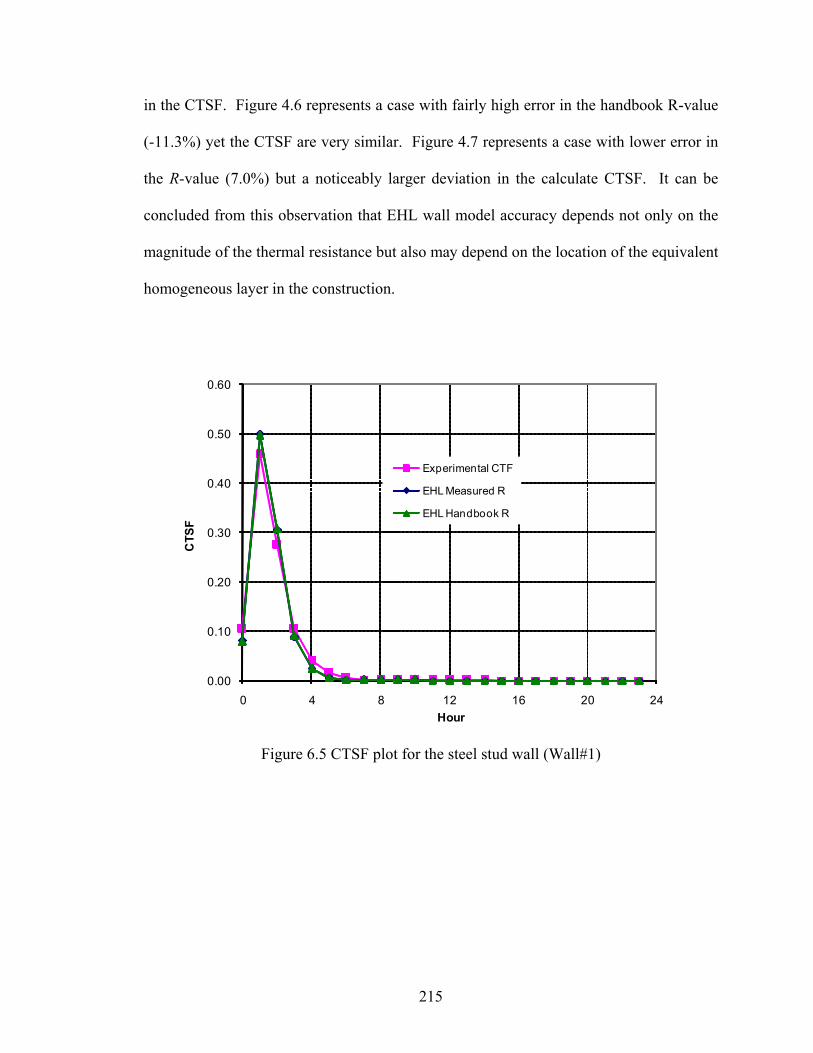
215
in the CTSF. Figure 4.6 represents a case with fairly high error in the handbook R-value
(-11.3%) yet the CTSF are very similar. Figure 4.7 represents a case with lower error in
the R-value (7.0%) but a noticeably larger deviation in the calculate CTSF. It can be
concluded from this observation that EHL wall model accuracy depends not only on the
magnitude of the thermal resistance but also may depend on the location of the equivalent
homogeneous layer in the construction.
0.00
0.10
0.20
0.30
0.40
0.50
0.60
0 4 8 12 16 20 24
CTS
F
Hour
Experimental CTF
EHL Measured R
EHL Handbook R
Figure 6.5 CTSF plot for the steel stud wall (Wall#1)
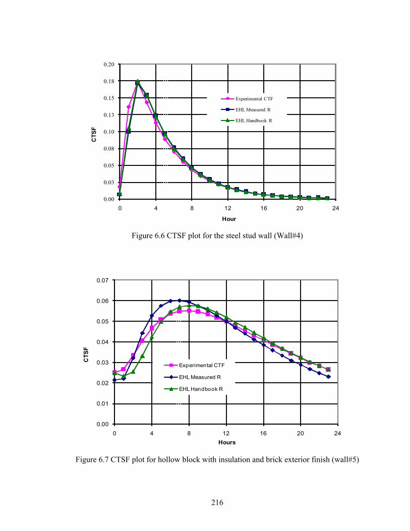
216
0.00
0.03
0.05
0.08
0.10
0.13
0.15
0.18
0.20
0 4 8 12 16 20 24
CTS
F
Hour
Experimental CTF
EHL Measured R
EHL Handbook R
Figure 6.6 CTSF plot for the steel stud wall (Wall#4)
0.00
0.01
0.02
0.03
0.04
0.05
0.06
0.07
0 4 8 12 16 20 24
CTS
F
Hours
Experimental CTF
EHL Measured R
EHL Handbook R
Figure 6.7 CTSF plot for hollow block with insulation and brick exterior finish (wall#5)
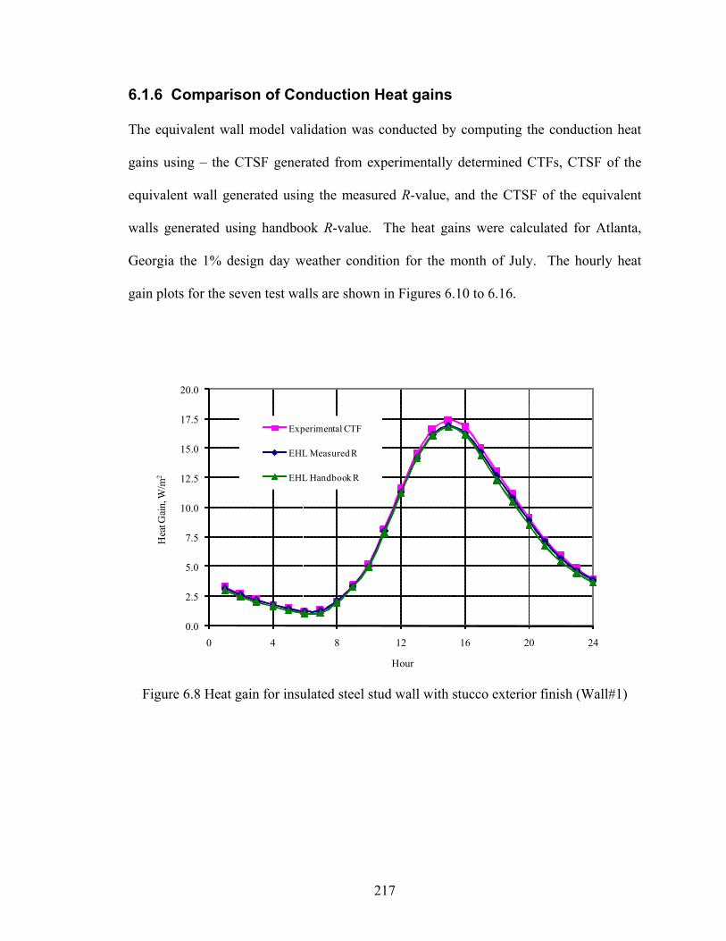
217
6.1.6 Comparison of Conduction Heat gains
The equivalent wall model validation was conducted by computing the conduction heat
gains using – the CTSF generated from experimentally determined CTFs, CTSF of the
equivalent wall generated using the measured R-value, and the CTSF of the equivalent
walls generated using handbook R-value. The heat gains were calculated for Atlanta,
Georgia the 1% design day weather condition for the month of July. The hourly heat
gain plots for the seven test walls are shown in Figures 6.10 to 6.16.
0.0
2.5
5.0
7.5
10.0
12.5
15.0
17.5
20.0
0 4 8 12 16 20 24
Hea
t Gai
n, W
/m2
Hour
Experimental CTF
EHL Measured R
EHL Handbook R
Figure 6.8 Heat gain for insulated steel stud wall with stucco exterior finish (Wall#1)
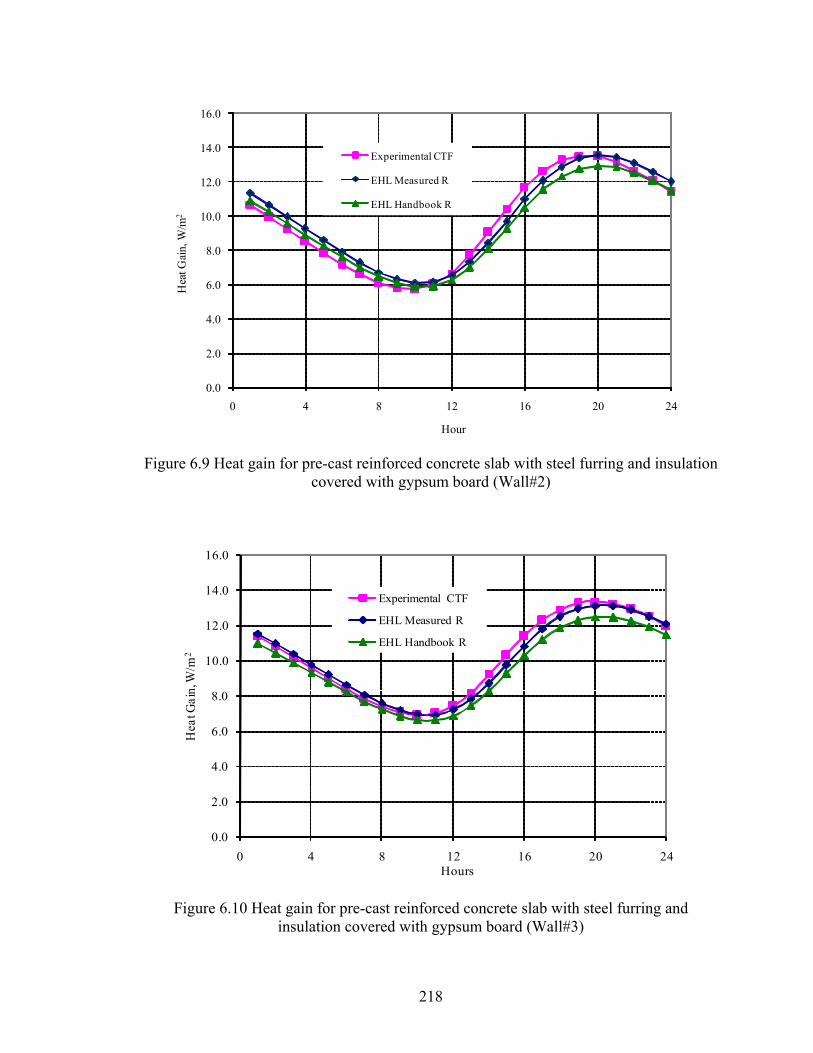
218
0.0
2.0
4.0
6.0
8.0
10.0
12.0
14.0
16.0
0 4 8 12 16 20 24
Hea
t Gai
n, W
/m2
Hour
Experimental CTF
EHL Measured R
EHL Handbook R
Figure 6.9 Heat gain for pre-cast reinforced concrete slab with steel furring and insulation
covered with gypsum board (Wall#2)
0.0
2.0
4.0
6.0
8.0
10.0
12.0
14.0
16.0
0 4 8 12 16 20 24
Hea
t Gai
n, W
/m2
Hours
Experimental CTF
EHL Measured R
EHL Handbook R
Figure 6.10 Heat gain for pre-cast reinforced concrete slab with steel furring and
insulation covered with gypsum board (Wall#3)
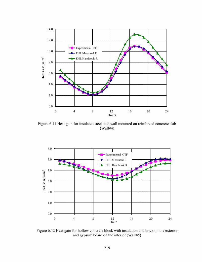
219
0.0
2.0
4.0
6.0
8.0
10.0
12.0
14.0
0 4 8 12 16 20 24
Hea
t Gai
n, W
/m2
Hours
Experimental CTF
EHL Measured R
EHL Handbook R
Figure 6.11 Heat gain for insulated steel stud wall mounted on reinforced concrete slab
(Wall#4)
0.0
1.0
2.0
3.0
4.0
5.0
6.0
0 4 8 12 16 20 24
Hea
t Gai
n, W
/m2
Hour
Experimental CTF
EHL Measured R
EHL Handbook R
Figure 6.12 Heat gain for hollow concrete block with insulation and brick on the exterior
and gypsum board on the interior (Wall#5)
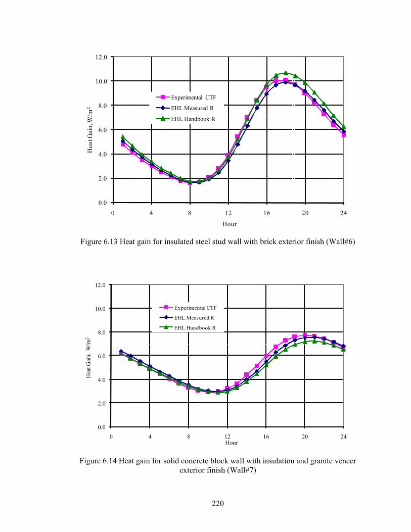
220
0.0
2.0
4.0
6.0
8.0
10.0
12.0
0 4 8 12 16 20 24
Hea
t Gai
n, W
/m2
Hour
Experimental CTF
EHL Measured R
EHL Handbook R
Figure 6.13 Heat gain for insulated steel stud wall with brick exterior finish (Wall#6)
0.0
2.0
4.0
6.0
8.0
10.0
12.0
0 4 8 12 16 20 24
Hea
t Gain
, W/m
2
Hour
Experimental CTF
EHL Measured R
EHL Handbook R
Figure 6.14 Heat gain for solid concrete block wall with insulation and granite veneer exterior finish (Wall#7)
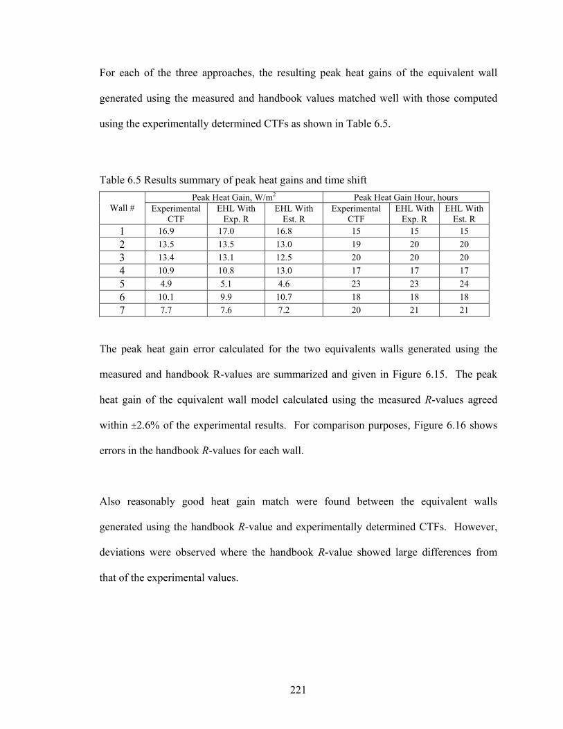
221
For each of the three approaches, the resulting peak heat gains of the equivalent wall
generated using the measured and handbook values matched well with those computed
using the experimentally determined CTFs as shown in Table 6.5.
Table 6.5 Results summary of peak heat gains and time shift Peak Heat Gain, W/m2 Peak Heat Gain Hour, hours
Wall # Experimental CTF
EHL With Exp. R
EHL With Est. R
Experimental CTF
EHL With Exp. R
EHL With Est. R
1 16.9 17.0 16.8 15 15 15 2 13.5 13.5 13.0 19 20 20 3 13.4 13.1 12.5 20 20 20 4 10.9 10.8 13.0 17 17 17 5 4.9 5.1 4.6 23 23 24 6 10.1 9.9 10.7 18 18 18 7 7.7 7.6 7.2 20 21 21
The peak heat gain error calculated for the two equivalents walls generated using the
measured and handbook R-values are summarized and given in Figure 6.15. The peak
heat gain of the equivalent wall model calculated using the measured R-values agreed
within ±2.6% of the experimental results. For comparison purposes, Figure 6.16 shows
errors in the handbook R-values for each wall.
Also reasonably good heat gain match were found between the equivalent walls
generated using the handbook R-value and experimentally determined CTFs. However,
deviations were observed where the handbook R-value showed large differences from
that of the experimental values.
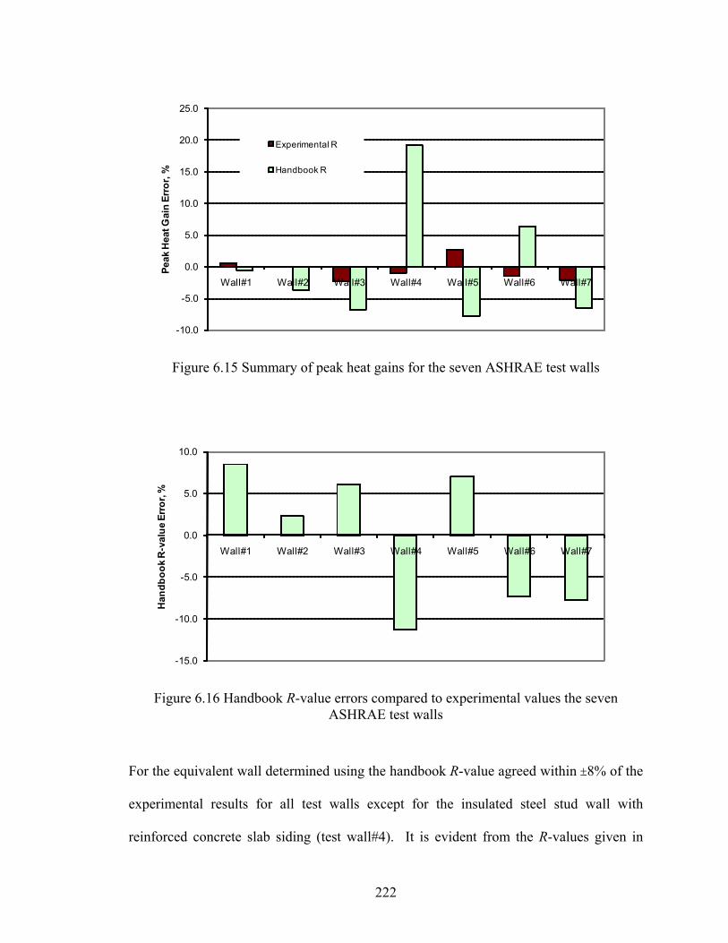
222
-10.0
-5.0
0.0
5.0
10.0
15.0
20.0
25.0
Wall#1 Wall#2 Wall#3 Wall#4 Wall#5 Wall#6 Wall#7
Peak
Hea
t Gai
n Er
ror,
%
Experimental R
Handbook R
Figure 6.15 Summary of peak heat gains for the seven ASHRAE test walls
-15.0
-10.0
-5.0
0.0
5.0
10.0
Wall#1 Wall#2 Wall#3 Wall#4 Wall#5 Wall#6 Wall#7
Han
dboo
k R
-val
ue E
rror
, %
Figure 6.16 Handbook R-value errors compared to experimental values the seven
ASHRAE test walls
For the equivalent wall determined using the handbook R-value agreed within ±8% of the
experimental results for all test walls except for the insulated steel stud wall with
reinforced concrete slab siding (test wall#4). It is evident from the R-values given in
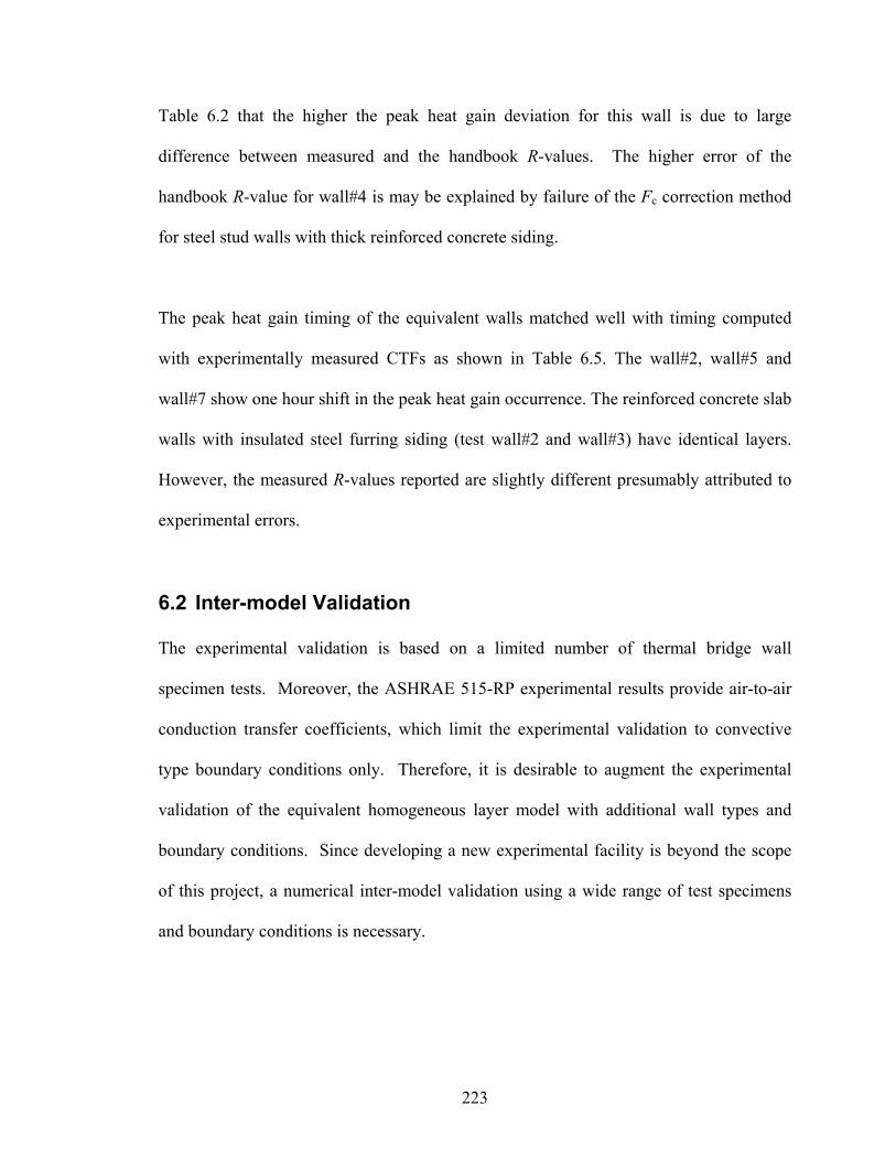
223
Table 6.2 that the higher the peak heat gain deviation for this wall is due to large
difference between measured and the handbook R-values. The higher error of the
handbook R-value for wall#4 is may be explained by failure of the Fc correction method
for steel stud walls with thick reinforced concrete siding.
The peak heat gain timing of the equivalent walls matched well with timing computed
with experimentally measured CTFs as shown in Table 6.5. The wall#2, wall#5 and
wall#7 show one hour shift in the peak heat gain occurrence. The reinforced concrete slab
walls with insulated steel furring siding (test wall#2 and wall#3) have identical layers.
However, the measured R-values reported are slightly different presumably attributed to
experimental errors.
6.2 Inter-model Validation
The experimental validation is based on a limited number of thermal bridge wall
specimen tests. Moreover, the ASHRAE 515-RP experimental results provide air-to-air
conduction transfer coefficients, which limit the experimental validation to convective
type boundary conditions only. Therefore, it is desirable to augment the experimental
validation of the equivalent homogeneous layer model with additional wall types and
boundary conditions. Since developing a new experimental facility is beyond the scope
of this project, a numerical inter-model validation using a wide range of test specimens
and boundary conditions is necessary.
224
The numerical validation is intended to augment the experimental validation and
demonstrate the suitability of implementation of the equivalent homogeneous layer wall
model in the one-dimensional energy analysis and load calculation programs. A two-
dimensional finite volume numerical method is used as a reference model for the inter
model validation. The validation has been done based on three generic steel stud
constructions identified by Gorgolewski (2007) and a wood stud wall. All the test
specimens in the numerical validation are sandwich type linear thermal bridges. The
description of the test walls is given next.
6.2.1 Numerical Validation Test Walls
Gorgolewski (2007) came up with three generic type steel stud walls commonly used in
building walls and roofs construction. These generic constructions were used as
representative test specimens for the numerical validation. For completeness wood stud
wall test specimen has been included. These test specimens are described next and their
construction layers thermo-physical properties are given in Table 6.6 and their section
views are shown in Figure 6.17.
Wood Stud Wall: the wood stud consists of wood siding on the exterior, after that
plywood, then a composite layer with fiberglass insulation and wood stud wall in parallel
and Gypsum interior finish. The stud has 88.9 mm depth and 38.1 mm width. The stud
center-to-center spacing is 406.4 mm. The actual wood stud wall layer is given in Table
6.6.
225
Table 6.6 Test walls layers description for inter-model validation
Layers Thickness (mm)
Conductivity (W/m⋅K)
Density (Kg/m3)
Specific Heat
(kJ/kg⋅K)
Resistance (m2⋅K /W)
Actual wall layers – wood stud wall Wood Siding 12.7 0.072 544.0 1.255 0.176 Plywood 12.7 0.115 544.0 1.213 0.110 Wood Stud 88.9 0.114 576.0 1.632 Fiber Glass Insulation 88.9 0.046 84.8 0.962 Gypsum 12.7 0.160 800.0 1.088 0.079 Actual wall layers – cold light steel stud wall Brick 102 0.720 1920.0 0.790 0.142 Clear Air Cavity 50 0.250 1.2 1.007 0.200 Plywood 20 0.115 544.0 1.213 0.174 Steel Stud 100 45.3 7600.0 0.500 Fiber Glass Insulation 100 0.029 14.5 0.710 Plaster Board 15 0.100 800.0 1.090 0.150 Actual wall layers – warm light steel stud wall Brick 102 0.720 1920.0 0.790 0.142 Clear Air Cavity 50 0.250 1.2 1.007 0.200 Rigid Insulation 50 0.046 84.8 0.962 1.087 Plywood 20 0.115 544.0 1.213 0.174 Steel Stud 100 45.3 7600.0 0.500 Air Gap 100 0.560 1.2 1.007 Plaster Board 15 0.100 800.0 1.090 0.150 Equivalent homogeneous layer wall – hybrid light steel stud wall Brick 102 0.720 1920.0 0.790 0.142 Clear Air Cavity 50 0.250 1.2 1.007 0.200 Rigid Insulation 50 0.046 84.8 0.962 1.087 Plywood 20 0.115 544.0 1.213 0.174 Steel Stud 100 45.3 7600.0 0.500 Fiber Glass Insulation 100 0.029 14.5 0.710 Plaster Board 15 0.100 800.0 1.090 0.150
Warm Frame Steel Stud Wall: the warm steel frame wall construction has no
insulation in between the steel studs and the insulation layer is on the exterior side. This
type of construction maintains the steel frame temperature close to the indoor air
temperature and is common for domestic design in the UK. The steel stud has 100 mm
depth, 38.1 mm width, 1.5 mm thickness and 609.6 mm center-to-center spacing. The
layer-by-layer description of the cold steel stud wall is given in Table 6.6.
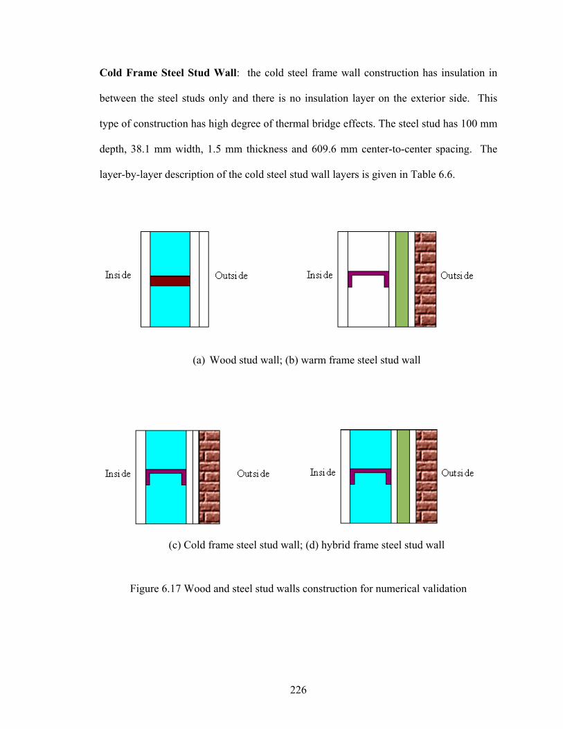
226
Cold Frame Steel Stud Wall: the cold steel frame wall construction has insulation in
between the steel studs only and there is no insulation layer on the exterior side. This
type of construction has high degree of thermal bridge effects. The steel stud has 100 mm
depth, 38.1 mm width, 1.5 mm thickness and 609.6 mm center-to-center spacing. The
layer-by-layer description of the cold steel stud wall layers is given in Table 6.6.
(a) Wood stud wall; (b) warm frame steel stud wall
(c) Cold frame steel stud wall; (d) hybrid frame steel stud wall
Figure 6.17 Wood and steel stud walls construction for numerical validation
227
Hybrid Frame Steel Stud Wall: the hybrid steel frame wall construction has insulation
on the exterior side and in between the steel stud layer. This is the most common type
construction used for domestic walls and roofs application (Gorgolewski 2007). The
steel stud has 100 mm depth, 38.1 mm width, 1.5 mm thickness and 609.6 mm center-to-
center spacing. The layer-by-layer description of the hybrid steel stud layer is given in
Table 6.6.
6.2.2 The R-values and The Equivalent Walls
The handbook surface-to-surface R-values of the wood stud and the steel stud walls were
calculated using the parallel path method and the Fc correction method, respectively, as
recommended by ASHRAE (2005). The R-values calculated using the 2D finite volume
numerical program, and ASHRAE’s recommended procedures are given in Table 6.7.
The equivalent wall generated of the four test walls are given in Table 6.8.
Table 6.7 Surface-to-surface R-values of the inter-model validation test walls (m2⋅K/W)
Test Walls 2D Finite Volume Method Handbook Handbook
Method Wood stud wall 2.10 2.09 Parallel Path Warm steel stud wall 1.95 1.91 Fc (=0.90) Cold steel stud wall 2.69 2.39 Fc (=0.55) Hybrid steel stud wall 3.92 3.59 Fc (=0.55)
228
Table 6.8 Equivalent walls for inter-model validation test walls
Layers Thickness (mm)
Conductivity (W/m⋅K)
Density (Kg/m3)
Specific Heat
(kJ/kg⋅K)
Resistance (m2⋅K /W)
Equivalent homogeneous layer wall – wood stud wall Wood Siding 12.7 0.072 544.0 1.255 0.176 Plywood 12.7 0.115 544.0 1.213 0.110 Equivalent layer 88.9 0.052 130.9 1.239 1.725 Gypsum 12.7 0.160 800.0 1.088 0.079 Equivalent homogeneous layer wall – warm light steel stud wall Brick 102 0.720 1920.0 0.790 0.142 Clear Air Cavity 50 0.250 1.2 1.007 0.200 Rigid Insulation 50 0.046 84.8 0.962 1.087 Plywood 20 0.115 544.0 1.213 0.174 Equivalent Layer 100 0.050 47.4 0.564 2.013 Plaster Board 15 0.100 800.0 1.090 0.150 Equivalent homogeneous layer wall – cold light steel stud wall Brick 102 0.720 1920.0 0.790 0.142 Clear Air Cavity 50 0.250 1.2 1.007 0.200 Plywood 20 0.115 544.0 1.213 0.174 Equivalent Layer 100 0.053 47.4 0.564 1.897 Plaster Board 15 0.100 800.0 1.090 0.150 Equivalent homogeneous layer wall – hybrid light steel stud wall Brick 102 0.720 1920.0 0.790 0.142 Clear Air Cavity 50 0.250 1.2 1.007 0.200 Rigid Insulation 50 0.046 84.8 0.962 1.087 Plywood 20 0.115 544.0 1.213 0.174 Equivalent Layer 100 0.050 47.4 0.564 2.013 Plaster Board 15 0.100 800.0 1.090 0.150
6.2.3 Performance of the Equivalent Walls
The steady periodic heat gains for the four test walls were determined using sol-air
temperature as boundary condition of ASHRAE’s 1% design day weather data of Atlanta,
Georgia. The hourly heat gains of the equivalent walls generated for R-values computed
using 2D finite volume numerical method and the handbook procedures and then
compared to that of a 2D transient finite volume numerical program. For the equivalent
walls the hourly heat gains were computed using conduction time series factors (CTSF)
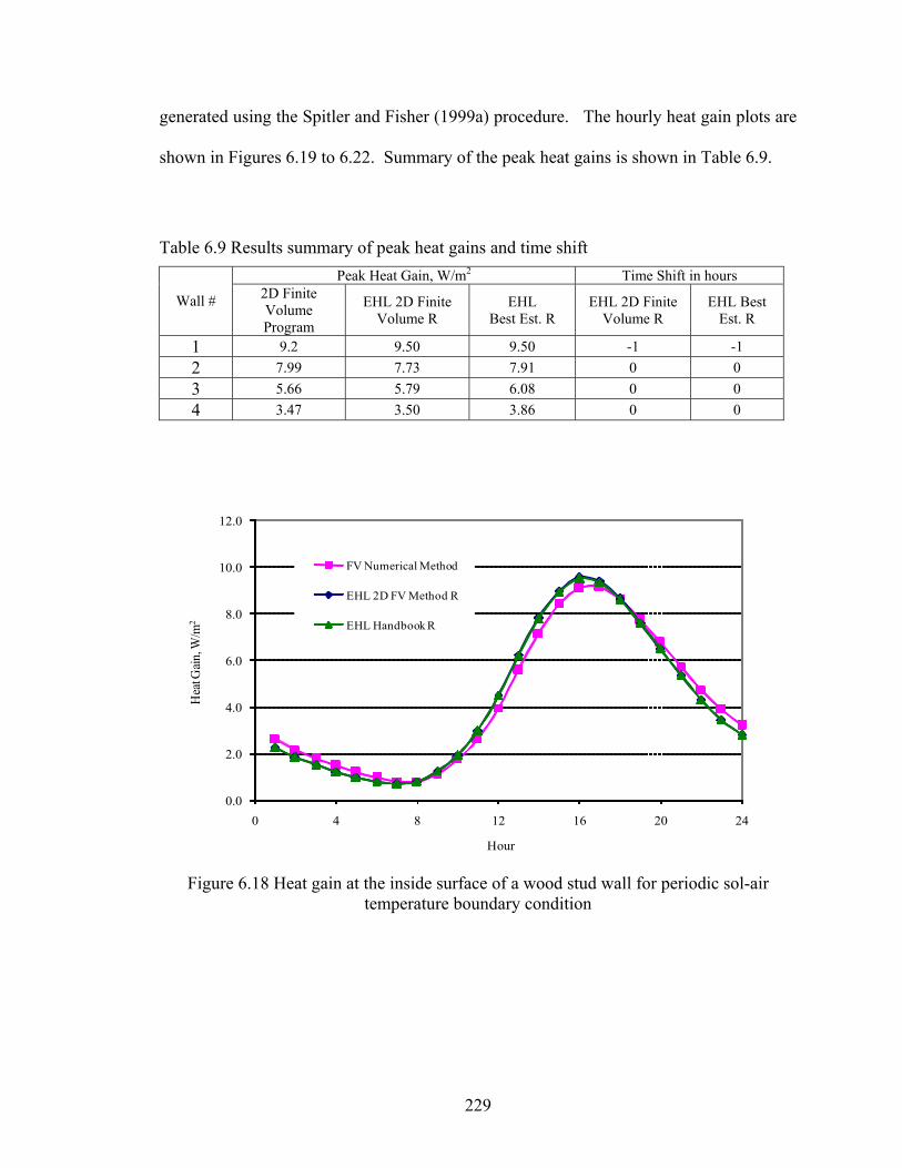
229
generated using the Spitler and Fisher (1999a) procedure. The hourly heat gain plots are
shown in Figures 6.19 to 6.22. Summary of the peak heat gains is shown in Table 6.9.
Table 6.9 Results summary of peak heat gains and time shift Peak Heat Gain, W/m2 Time Shift in hours
Wall # 2D Finite Volume Program
EHL 2D Finite Volume R
EHL Best Est. R
EHL 2D Finite Volume R
EHL Best Est. R
1 9.2 9.50 9.50 -1 -1 2 7.99 7.73 7.91 0 0 3 5.66 5.79 6.08 0 0 4 3.47 3.50 3.86 0 0
0.0
2.0
4.0
6.0
8.0
10.0
12.0
0 4 8 12 16 20 24
Hea
t Gain
, W/m
2
Hour
FV Numerical Method
EHL 2D FV Method R
EHL Handbook R
Figure 6.18 Heat gain at the inside surface of a wood stud wall for periodic sol-air
temperature boundary condition
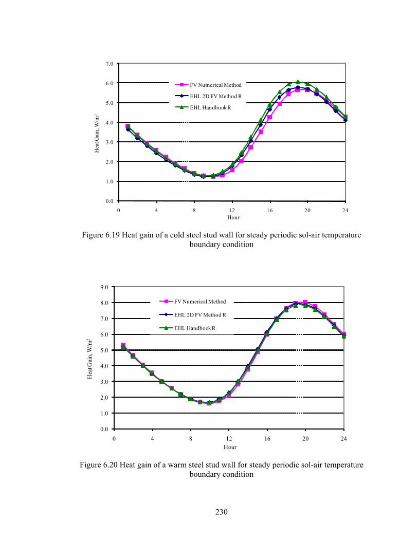
230
0.0
1.0
2.0
3.0
4.0
5.0
6.0
7.0
0 4 8 12 16 20 24
Hea
t Gai
n, W
/m2
Hour
FV Numerical Method
EHL 2D FV Method R
EHL Handbook R
Figure 6.19 Heat gain of a cold steel stud wall for steady periodic sol-air temperature
boundary condition
0.0
1.0
2.0
3.0
4.0
5.0
6.0
7.0
8.0
9.0
0 4 8 12 16 20 24
Hea
t Gai
n, W
/m2
Hour
FV Numerical Method
EHL 2D FV Method R
EHL Handbook R
Figure 6.20 Heat gain of a warm steel stud wall for steady periodic sol-air temperature
boundary condition
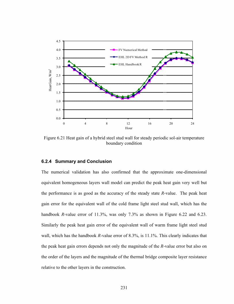
231
0.0
0.5
1.0
1.5
2.0
2.5
3.0
3.5
4.0
4.5
0 4 8 12 16 20 24
Hea
t Gain
, W/m
2
Hour
FV Numerical Method
EHL 2D FV Method R
EHL Handbook R
Figure 6.21 Heat gain of a hybrid steel stud wall for steady periodic sol-air temperature
boundary condition
6.2.4 Summary and Conclusion
The numerical validation has also confirmed that the approximate one-dimensional
equivalent homogeneous layers wall model can predict the peak heat gain very well but
the performance is as good as the accuracy of the steady state R-value. The peak heat
gain error for the equivalent wall of the cold frame light steel stud wall, which has the
handbook R-value error of 11.3%, was only 7.3% as shown in Figure 6.22 and 6.23.
Similarly the peak heat gain error of the equivalent wall of warm frame light steel stud
wall, which has the handbook R-value error of 8.3%, is 11.1%. This clearly indicates that
the peak heat gain errors depends not only the magnitude of the R-value error but also on
the order of the layers and the magnitude of the thermal bridge composite layer resistance
relative to the other layers in the construction.
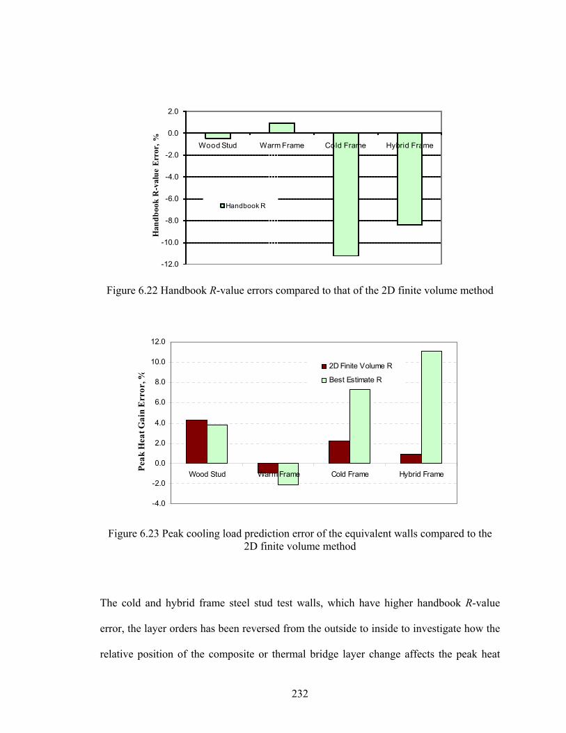
232
-12.0
-10.0
-8.0
-6.0
-4.0
-2.0
0.0
2.0
Wood Stud Warm Frame Cold Frame Hybrid FrameH
andb
ook
R-v
alue
Err
or,%
Handbook R
Figure 6.22 Handbook R-value errors compared to that of the 2D finite volume method
-4.0
-2.0
0.0
2.0
4.0
6.0
8.0
10.0
12.0
Wood Stud Warm Frame Cold Frame Hybrid Frame
Peak
Hea
t Gai
n E
rror
, %
2D Finite Volume R
Best Estimate R
Figure 6.23 Peak cooling load prediction error of the equivalent walls compared to the
2D finite volume method
The cold and hybrid frame steel stud test walls, which have higher handbook R-value
error, the layer orders has been reversed from the outside to inside to investigate how the
relative position of the composite or thermal bridge layer change affects the peak heat
233
gain prediction of the equivalent wall. The reversed layers order equivalent walls are
identical since the steady state R-values are the same. For the reversed layers order the
cold and hybrid steel stud equivalent walls peak heat gains reduced to 5.0% and 10.2%
from 7.3% and 11.1%, respectively. This change in the peak heat gain error shows how
the relative position of the thermal bridge composite layer may affect the peak heat gain
prediction performance of the equivalent wall. It can be inferred from these that it is
essential to maintain the number of layers and the layers order as in the actual
construction whenever possible.
The equivalent wall model predicts the peak cooling load within ±2.5% of a 2D finite
numerical program provided the steady state R-values are determined using two-
dimensional numerical programs. In fact this suggests that a numerical program that can
generate equivalent walls can be developed and readily integrated into existing one-
dimensional energy analysis and load calculation programs. However, this requires a
standalone 2D user interface for construction geometry and material layer specification to
compute accurate steady state R-value and then generate the equivalent wall.
6.3 Conclusion and Recommendations
The experimental and the inter-model validations have confirmed that the equivalent
homogeneous layer wall model can replicate the peak heat gains of walls with thermal
bridges with the accuracy primarily limited by the estimate of the R-values. This has
been demonstrated using the seven ASHRAE RP-515 test walls and a wood stud wall,
and three generic type steel frame walls identified by Gorgolewski (2007).
234
When measured R-values are used, the EHL model agreed within ±2.6% of the
experimental results. When standard methods recommended by ASHRAE for estimating
the R-values were used, the peak heat gains for six of walls were predicted within ±7.7%
of the peak heat gain determined using the measured CTFs. For the seventh wall, an
insulated steel stud wall mounted on reinforced concrete slab, a peak heat gain error of
19.3% was observed. This is primarily due to an 11.3% deviation of the handbook R-
value from the measured R-value.
The inter-model validation also confirmed that the equivalent wall for light steel stud
walls predicts the peak heat gain within ±2.5% of that of the actual wall provided that the
R-values were determined using the 2D numerical model. The errors in the R-values for
the numerical test walls computed with standard method were in the range 0.5% to
11.3%. For the cold frame steel stud test wall with the R-value error of 11.3%, the peak
heat gain error was 7.3%.
It can be concluded from experimental and numerical validation that the EHL walls
duplicate the dynamics of walls with thermal bridges provided the thermal resistances of
the actual construction and the thermal mass of the composite layer are predicted
accurately and the layers order are maintained as in the actual wall. It can be said that the
equivalent homogeneous layer dynamic model is as good as the accuracy of the R-value
estimate.
235
The EHL wall model accuracy dependency on the layers order has been investigated by
reversing layers order for cold and hybrid steel stud test walls. The reversed layer and
the actual walls have the same R-values. Interestingly, reversing layers order brought
31.5%, and 8.1%, respectively, reduction in the peak heat gain prediction error. This
clearly indicates that the EHL wall model performance also slightly depends on the
location of the thermal bridge layer relative to highly resistive and massive layers in the
construction.
General Recommendation
The following guidelines are additional recommendation that help to improve
implementation of the equivalent homogeneous layer wall model to thermal bridges:
i. Maintain the number of layers and the layer order in the actual wall construction
as much as possible. Otherwise, it is recommended to keep at least three
homogeneous layers in the equivalent wall whenever possible.
ii. The overall thickness of the equivalent wall must be the same as that of the actual
wall and the thermal mass and the sequence must correspond to each layer in the
actual construction.
iii. Air gaps adjacent to composite layers should remain as a separate layer unless
elements of the composite layers such as tie-rods, screws or bolts protrude into the
air gap layer. In the later case combine the air gap with composite layer. Then
the thickness of the equivalent homogeneous layer is the sum of the composite
layers and that of the air gap thickness. The thermal mass of the equivalent layer
must then include that of the air gap as well.
236
iv. If the composite layer has significant thermal mass difference along the principal
heat flow direction then divide the composite layer into two homogeneous layers
reflecting the realistic thermal mass distributions.
v. If there are two composite layers separated by homogeneous layers, then there
must be two equal homogeneous layers one for each. Then, the equivalent layers
will be apportioned based on the thermal resistance ratio of the dominant elements
in the two composite layers. But the equivalent layers thermal masses should be
based on the actual constructions in each composite layer.
vi. The reinforcement metal bars in the concrete slab can be ignored in the thermal
resistance calculation. Treat the concrete slab as if it is homogeneous layer but
correct the thermal mass for the effect of the reinforcement bar.
6.4 Recommendation for Future Work
The equivalent homogeneous layer wall model is suited only for sandwich type thermal
bridge constructions. Two limitations of the equivalent homogeneous layer wall model
that has been identified: when thermal bridge element is exposed to interior or exterior
environments, and when multiple composite layers are separated by homogeneous layer
in sandwich type thermal bridges. The multi-composite layers can be lumped together.
But this needs to be validated either experimentally or numerically. Therefore, these two
limiting cases of the equivalent homogeneous layer wall model require further
investigation hence are recommended as a future work.
237
CHAPTER VII
7 Conclusions and Recommendations
In this thesis a series of investigations of the Radiant Time Series Method (RTSM) have
been conducted, in some cases leading to improvements to the method, its sub-models,
supporting data, or facilitation of implementation in a wide range of computing
environments. These developments include:
1. The improved RTSM procedure, which accounts for transmission of radiant heat
gains back to the outside by conduction through fenestration or other high
conductance surfaces.
2. Modification of fenestration model: adapted the RTSM to use recent developments
in fenestration models and data. A new set of radiative / convective splits have
been established.
3. Development of the reduced heat balance method for RTF generation.
4. Development of simplifications to facilitate implementation of the RTSM in a range
of computing environments.
5. Parametric investigation to establish the limitations of the RTSM and provide
design guidance.
238
Furthermore, an approximate one-dimensional dynamic model for thermal bridges has
been investigated and design guidance for practicing engineers has been established. The
dynamic model of thermal bridges can be used with other energy analysis and load
calculation procedures as well in the following sections, conclusions based on the
findings are summarized and recommended future works are presented.
7.1 Improvement to the Radiant Time Series Method
The improvements of the RTSM procedure correspond to the first four developments
listed above. The findings are summarized in the following sections:
7.1.1 Accounting for Heat Losses in RTSM
An algorithm for correcting the space radiant heat gains to account for radiant loss by
conduction has been derived as discussed in Section 3.3.1. The procedure accounts for
solar and internal radiant heat gains conducted back out through fenestrations. The
algorithm is formulated using a dimensionless loss conductance that can easily be
computed from the fenestration U-value, inside combined conductance and total area of
the zone surfaces including furnishings. The procedure has been implemented by
correcting the first term of the radiant time factors and hence maintains the simplicity
desired in the RTSM procedure. The peak cooling load over prediction trend of the
RTSM procedure has been improved dramatically, as discussed below in section 7.1.5.
With this addition, the current RTSM procedure is referred to as the improved RTSM
procedure.
239
7.1.2 Improvements to the RTSM Fenestration Model
The RTSM fenestration models have been adapted to the use of solar heat gain
coefficients (SHGC) currently available from window manufacturers and interior
attenuation coefficients (IAC) as appear in the current (2005) ASHRAE Handbook of
Fundamentals. Since SHGC do not give information about the split between transmitted
and absorbed components, as was available with previous models which used shading
coefficients, new radiative / convective splits were needed. These were determined with
a parametric study described in Section 3.2 and are summarized in Table 3.5. The
performance of the new set of radiative / convective splits has been characterized with
parametric investigation summarized in Section 7.1.5.
7.1.3 Improvements to the RTF generation
An algorithm for generating Radiant Time Factors (RTF) based on the reduced heat
balance procedure has been derived, as discussed in Section 3.1, and validated against a
full-blown heat balance program. The new RTF engine uses periodic response factors,
which are generated from conduction transfer functions (CTFs) computed using the state
space method. The reduced heat balance method eliminates the unneeded features in the
HBM, such as the outside heat balance and treatment of solar radiation, and it uses
compact matrix notation. Hence implementation of the method can take advantage of
programming environments with built-in matrix algebra or matrix algebra libraries.
Furthermore, a constant radiation use in the system matrix has been investigated, which
may reduces the RTF generation time by one-halt without loss of accuracy. This is
desirable for implementation in VBA.
240
7.1.4 Developments in RTSM Implementations
Implementation of the RTSM in different computing environments has been hindered by
computational efforts required to generate the periodic response factors (PRF) and the
radiant time factors (RTF). Specifically, the RTSM was intended for use as a spreadsheet
method, yet it originally required a full-blown HBM program to generate the PRF and
RTF. The developments to facilitate implementations of the RTSM in other computing
environments are summarized as follows:
An alternative procedure for generating periodic response factors (PRF) that uses a
one-dimensional finite volume numerical method has been developed and
successfully implemented in VBA and FORTRAN 90. This algorithm has some
advantages over the Laplace and State Space methods in that it’s based on
fundamental concepts understandable by senior level undergraduate students and is
suitable for implementation in any computational platform. In particular its
suitability for use with VBA is convenient for implementation of the RTSM in
spreadsheets.
The reduced HBM RTF generation algorithm has also been implemented in VBA
and SCILAB. Its implementation in VBA makes the RTSM entirely a “spreadsheet
procedure” – thus no external DLL or other computer programs are needed.
7.1.5 Parametric Study of the Performance of RTSM
Performance of the current and improved RTSM procedures has been investigated using
a total of 2,867,200 zones representing a wide range of building constructions, zone
geometries, fenestrations with and without interior shading, and design weather and
241
locations. In the discussion below, the term “current RTSM” refers to the original RTSM
(Spitler et al. 1997) procedure with the new fenestration model. The term “Improved
RTSM” procedure refers to the current RTSM with heat loss correction applied. This
investigation was intended to establish the limitations of the RTSM peak cooling
prediction quantitatively as design guidance for practicing engineers. The following
conclusions can be deduced from the parametric investigations conducted:
The extreme peak cooling over prediction trend of the RTSM procedure showed
strong dependency on:
glazing fraction – over prediction increases with glazing fraction
glazing types – high SHGC increases the amount of solar heat gain for
unshaded fenestration and hence increases the over prediction
peak design temperature – lower peak design temperatures tend to increase
the peak cooling over prediction
zone orientation – zones in the east and north-east zones tend to peak in
the morning, hence tending to increase the over prediction
number of exterior facade surfaces – increasing the exterior facades
increases in the over predictions
interior shades – reduce the amount of solar heat gain and hence reduce
the peak cooling load over prediction
construction fabric – without interior shaded fenestration, light and
heavyweight construction tend to have the same over predictions.
However, for zones with interior shaded fenestration, heavyweight
construction zones tend to result in higher overpredict than lightweight
242
zone construction. This not endemic to the method but is an effect of the
single radiative fraction for all SHGC applied to all zones.
The improved RTSM procedure reduced the over prediction of peak cooling load
significantly, in particular for fenestrations without interior shades. For 716,800
zones without interior shading, the current RTSM over predictions are as high as
30.5% while it is reduced to 10.5% for the improved RTSM procedure. The
maximum over prediction occurs for zones with single pane clear glass on two
exterior facade surfaces. The over prediction for other glazing types and zone
constructions are summarized in Table 4.10.
The average over prediction of peak cooling load of the current RTSM for 71,680
zones at 50% and 71,680 zones at 90% exterior facade glazing fraction for
fenestration without interior shades are 8.4% and 12.7%, respectively. Overall the
improved RTSM gives substantially lower over predictions for the entire range of
problem zones. The average over predictions for the same 71,680 zones reduced to
5.6% and 4.5%, respectively.
The over prediction is smaller when the fenestration has interior shades due to
reduction in the amount of solar heat gain. The maximum over predictions of the
current and improved RTSM procedures for 716,800 zones with interior shade
fenestration are 19.9% and 17.7%, respectively. For the current RTSM procedure
this occurs at 90% glazing fraction of the exterior facade. The average
overpredictions of the current RTSM procedure for zones with interior shaded
fenestration at 50% (71,680 zones) and 90% (71,680 zones) glazing fractions are
243
10.3% and 12.8%, respectively. The improved RTSM procedure only reduces the
average over predictions of peak cooling load for these zones to 8.6% and 9.8%,
respectively.
As the result of the use of a fixed radiative fraction for all construction fabrics, the
RTSM peak cooling load over prediction is different with light and heavyweight
constructions. Peak cooling load over predictions for zones with shaded windows
tend to be higher for heavyweight zones than lightweight zones by 2% - 12%
depending on the glazing type. The over prediction trends for different glazing
types are summarized in Table 4.11.
7.2 Conclusions: Dynamic Modeling of Thermal Bridges
The approximate one-dimensional procedure, the equivalent homogeneous layer (EHL)
wall model, proposed by Karambakkam et al. (2005) has been validated against
experimental results published by Brown and Stephenson (1993a; 1993b). As the
experimental validation test specimens were limited to seven test walls, a wood stud wall
and three generic steel stud walls identified by Gorgolewski (2007) have been validated
against a 2D finite volume program. Brown and Stephenson derived conduction transfer
functions (CTFs) for each wall. These CTFs and the conduction time series factors
(CTSFs) developed with the equivalent homogeneous layer (EHL) wall model were used
to compare peak heat gains for a typical sol-air temperature profile. For inter-model
validation using 2D finite volume program, peak heat gains computed with EHL-model
derived CTFs were compared to peak heat gains computed directly with 2D finite volume
244
program. The following conclusions can be drawn from the experimental and inter-
model validations:
The experimental and the inter-model validations have confirmed that the
equivalent homogeneous layer wall model can replicate the peak heat gains of
walls with thermal bridges with the accuracy primarily limited by the estimate of
the R-values.
When measured R-values are used, the EHL model agreed within ±2.6% of the
experimental results. When standard methods recommended by ASHRAE for
estimating the R-values were used, the peak heat gains for six of walls were
predicted within ±7.7% of the peak heat gain determined using the measured
CTFs. For the seventh wall, an insulated steel stud wall mounted on reinforced
concrete slab, a peak heat gain error of 19.3% was observed. This is primarily
due to an 11.3% deviation of the handbook R-value from the measured R-value.
The inter-model validation also confirmed that the equivalent wall for the steel
stud walls predicts the peak heat gain within ±2.5% of that of the actual wall
provided that the R-values were determined using the 2D numerical model. The
errors in the R-values computed with standard method were in the range 0.5% to
11.3%. For the cold frame steel stud test wall with the R-value error of 11.3%,
the peak heat gain error was 7.3%.
In its current form, the equivalent homogeneous layer wall model is suitable for
sandwich type linear thermal bridge constructions with one composite layer only.
For walls with multiple composite layers, the resistance would have to be
apportioned. It is expected that this will work well but has not been validated.
245
The use of either air-to-air or surface-to-surface R-values for equivalent wall
generation depends on the procedure used to determine the overall R-value or U-
values. For R-values determined using either isothermal plane or the parallel path
correction method the use of either R-value gives the same equivalent
homogeneous layer. For R-values determined using the parallel path or zone
methods the properties of the EHL wall vary slightly depending on whether the
basis is air-to-air or surface-to-surface R-values. If the parallel path extends to
air-to-air node in the R-value calculation then the air-to-air R-value should be
used in the equivalent layer determination. If the parallel path method combines
the facing layers in series with composite layer then the use of either air-to-air or
surface-to-surface R-values gives the same equivalent layer.
7.3 Recommendations for Future Work
The recommendations for future work involving improvements to the radiant time series
method or dynamic modeling of thermal bridges can be summarized as follows:
The radiative / convective splits recommended for use with the RTSM
fenestration models were based on interior shades with maximum transmittance of
10%. Since some shades, such as light and medium weave drapery fabrics, have
higher transmittance, further investigation of radiative / convective splits for
higher transmittance interior shades is recommended.
The improved RTSM peak cooling load over prediction may be reduced further
with the use of radiative / convective split that depends on the glazing types,
246
construction fabrics, and glazing fractions. Investigation of such a correlation is
recommended.
Validation of use of constant radiation coefficient in RTF generation algorithm
for large set of zones is recommended for future work.
A parametric study to cover the three generic steel stud walls with different stud
spacings, flange widths and thicknesses and different levels of insulation is
recommended as future work.
The equivalent homogeneous layer wall model as is cannot be used for exposed
type thermal bridges. Exposed type thermal bridges may be found in some
curtain wall constructions. Extension of the model for exposed type layer thermal
bridge construction is recommended for future work.
Furthermore, while multiple composite layers separated by homogeneous layers
may be analyzed by apportioning the resistance between the two layers, this
approach has not been validated. This validation should be done.
The experimental and inter-model validation of the equivalent homogeneous
conducted so far have been using design oriented sol-air temperature boundary
conditions. It is recommended for future work to validate the model with other
types of boundary conditions involving a combination of solar, long wave and
convective environments.
The one-dimensional approximate equivalent homogenous layers wall model can
be implemented as a standalone tool and/or can be integrated with existing
building energy analysis and load calculation programs. This would require a two
dimensional numerical model with a graphical user interface for geometrical and

247
material layer specifications, and a sub-program for solving the two-dimensional
conduction domain to determine the steady state R-value and generate the one-
dimensional equivalent wall. Such a tool, if developed with practicing engineers
in mind, would be quite useful and efforts to develop this tool should be
undertaken.

248
249
REFERENCES
Alford, J. S., L. Mass, J.E. Ryan, N.Y. Schenectady, F.O. Urban, and Bloomfield, N. J.
(1939). “Effect of Heat Storage and Variation in Outdoor Temperature and Solar
Intensity on the Heat Transfer Through Walls." ASHVE Transactions, 45(1), 369-
396.
Amjad, S., Abdelbaki, A., and Zrikem, Z. (2003). "Transfer functions method and sub-
structuration technique for two-dimensional heat conduction problems in high
thermal mass systems: Application to ground coupling problems." Energy and
Buildings, 35(6), 593-604.
ASHRAE. (1967). Handbook of Fundamentals, Atlanta: American Society of Heating,
Refrigerating, and Air-Conditioning Engineers, Inc.
ASHRAE. (1972). Handbook of Fundamentals, Atlanta: American Society of Heating,
Refrigerating, and Air-Conditioning Engineers, Inc.
ASHRAE. (2001). Handbook of Fundamentals, Atlanta: American Society of Heating,
Refrigerating, and Air-Conditioning Engineers, Inc.
ASHRAE. (2005). Handbook of Fundamentals, Atlanta: American Society of Heating,
Refrigerating, and Air-Conditioning Engineers, Inc.
Barbour, C. E., and Goodrow, J. "Thermal performance of steel-framed walls." San
Diego, CA, USA, 766-777.
250
Billington, N. S. (1987). "Evolution of Environmental Temperature." Building and
Environment, 22(4), 241-249.
Brisken, W. R., and Reque, S. G. (1956). " Heat Load Calculations by Thermal
Response." ASHVE Transactions, 62(1), 391-424.
Billington, N. S. (1987). "Evolution of Environmental Temperature." Building and
Environment, 22(4), 241-249.
Brisken, W. R., and Reque, S. G. (1956). " Heat Load Calculations by Thermal
Response." ASHVE Transactions, 62(1), 391-424.
Brown, W. C., and Stephenson, D. G. (1993a). "Guarded hot box measurements of the
dynamic heat transmission characteristics of seven wall specimens - Part II."
ASHRAE Transactions, 99(1), 643-660.
Brown, W. C., and Stephenson, D. G. (1993b). "Guarded hot box procedure for
determining the dynamic response of full-scale wall specimens - Part I." ASHRAE
Transactions, 99(1), 632-642.
Brown, W. C., Swinton, M. C., and Haysom, J. C. (1998). "Technique for calculating the
effective thermal resistance of steel stud walls for code compliance." ASHRAE
Transactions, 104(2), 1245-1255.
Burch, D. M., Seem, J. E., Walton, G. N., and Licitra, B. A. (1992). "Dynamic evaluation
of thermal bridges in a typical office building." ASHRAE Transactions, 98(1),
291-304.
Carpenter, S. C., Kosny, J., and Kossecka, E. (2003a). "Modeling Transient Performance
of Two-Dimensional and Three-Dimensional Building Assemblies." ASHRAE
Transactions, 2003, 561-566.
251
Carpenter, S. C., Kosny, J., and Kossecka, E. "Modeling transient performance of two-
dimensional and three-dimensional building assemblies." Chicago, IL, United
States, 566-571.
Carpenter, S. C., and Schumacher, C. (2003). "Characterization of framing factors for
wood-framed low-rise residential buildings." ASHRAE Transactions, 109(1), 101-
108.
Carroll, J. A. (1980). "An "MRT Method" of Computing Radiant Energy Exchange in
Rooms." San Diego, California, 343-348.
Carslaw, H. S., and Jaeger, J. C. (1959). Conduction of heat in solids, Oxford, Clarendon
Press, London.
Chantrasrisalai, C., and Fisher, D. E. (2007a). "Lighting heat gain parameters:
Experimental method (RP-1282)." HVAC and R Research, 13(2), 283-303.
Chantrasrisalai, C., and Fisher, D. E. (2007b). "Lighting heat gain parameters:
Experimental results (RP-1282)." HVAC and R Research, 13(2), 305-323.
Chantrasrisalai, C., Iu, I., Eldridge, D. S., and Fisher, D. E. (2003). "Experimental
validation of design cooling load procedures: The heat balance method." ASHRAE
Transactions, 109 (2), 160-173.
Chen, Y., and Wang, S. (2005). "A new procedure for calculating periodic response
factors based on frequency domain regression method." International Journal of
Thermal Sciences, 44(4), 382-392.
Clarke, J. A. (2001). Energy Simulations in Building Design, Butterworth-Heinemann. .
252
Davies, M., Tindale, A., and Littler, J. (1995). "Importance of multi-dimensional
conductive heat flows in and around buildings." Building Services Engineering
Research & Technology, 16(2), 83-90.
Davies, M. G. (1996). "Time-domain estimation of wall conduction transfer function
coefficients." ASHRAE Transactions, 102(1), 328-343.
Fisher, D. E., and Chantrasrisalai, C. (2006). "Lighting Heat Gain Distribution In
Buildings." Georgia, Atlanta.
Gilkey, H. T., D. R. Bahnfleth, and Roose, R. W. (1953). "Cooling a Small Residence
House with a Two-Horse Power Mechanical Condensing Unit." ASHVE
Transactions, 59(1), 283-304.
Gorgolewski, M. (2007). " Developing a simplified method of calculating U-values in
light steel framing." Building and Environment, Volume 42(1), 230-236.
Hittle, D. C. (1992). "Response Factors and Conduction Transfer Functions." 1-42.
Hottel, H. C., and Sarofim, A. F. (1967). Radiation Transfer, McGraw-Hill, New York.
Houghten, F. C., J. C. Blackshaw, E. M. Pugh, and McDermott, P. (1932). "Heat
Transmission as Influenced by Heat Capacity and Solar Radiation." ASHVE
Transactions, 38(1), 232-284.
Iu, I., Eldridge, D. S., Chantrasrisalai, C., and Fisher, D. E. (2003). "Experimental
validation of design cooling load procedures: The radiant time series method."
ASHRAE Transactions, 109(2), 139-150.
James, J. (1937). " Cooling Load Analysis of A Bank." ASHVE Transactions, 43(1), 327–
344.
253
Karambakkam, B. K., B. Nigusse, and Spitler, J. D. "A One-dimensional Approximation
for Transient Multi-dimensional Conduction Heat Transfer in Building
Envelopes. ." Nordic Symposium on Building Physics, Reykjavík, Iceland.
Kayan, C. F. (1950). "Electric Analogger Studies on Panels with Embedded Tubes."
ASHVE Transactions, 56(1), 205-222.
Klems, J. H. (2002). "Solar heat gain through fenestration systems containing shading:
Summary of procedures for estimating performance from minimal data."
ASHRAE Transactions, 108(1), 512-524.
Kosny, J., and Christian, J. E. "Reducing the uncertainties associated with using the
ASHRAE zone method for R-value calculations of metal frame walls." San
Diego, CA, USA, 779-788.
Kosny, J., and Christian, J. E. (1995b). "Reducing the uncertainties associated with using
the ASHRAE zone method for R-value calculations of metal frame walls."
ASHRAE Transactions, 101(2), 779-788.
Kosny, J., and Christian, J. E. (1995c). "Thermal evaluation of several configurations of
insulation and structural materials for some metal stud walls." Energy and
Buildings, 22(2), 157-163.
Kosny, J., Christian, J. E., and Desjarlais, A. O. (1997a). "Metal stud wall systems -
thermal disaster, or modern wall systems with highly efficient thermal insulation."
1320, 153-179.
Kosny, J., Christian, J. E., and Desjarlais, A. O. (1997b). "Thermal breaking systems for
metal stud walls - can metal stud walls perform as well as wood stud walls?"
ASHRAE Transactions, 103(1), 518-536.
254
Kosny, J., and Kossecka, E. (2002). "Multi-dimensional heat transfer through complex
building envelope assemblies in hourly energy simulation programs." Energy and
Buildings, 34(5), 445-454.
Kosny, J., Petrie, T. W., and Christian, J. E. (1997c). "Thermal bridges in roofs made of
wood and light-gauge steel profiles." ASHRAE Transactions, 103(1), 537-549.
Kossecka, E. (1998). "Relationships between structure factors, response factors, and z-
transfer function coefficients for multilayer walls." ASHRAE Transactions,
104(1), 68-77.
Kossecka, E., and Kosny, J. (2002). "Influence of insulation configuration on heating and
cooling loads in a continuously used building." Energy and Buildings, 34(4), 321-
331.
Kratz, A. P., and Konzo, S. (1933). "Study of Summer Cooling in the Research
Residence at the University of Illinois." ASHVE Transactions, 39(1), 95 –118.
Kusuda, T. (1969). "Thermal Response Factors for Multi-layered Structures of Various
Heat Conduction systems. ." ASHRAE Transactions, 75(Pt 1), 241-271.
Leopold, C. S. (1948). "Hydraulic Analogue For The Solution of Problems of Thermal
Storage, Radiation, Convection, and Conduction." ASHVE Transactions, 54(1),
391-424.
Mackey, C. O., and Wright, L. T. (1944). "Periodic Heat Flow-Homogeneous Walls or
Roofs." Transactions American Society of Heating and Ventilating Engineers,
50(1), 293-312.
Mackey, C. O., and Wright, L. T. (1946). "Periodic Heat Flow-Composite Walls or
Roofs." Transactions American Society of Heating and Ventilating Engineers,
52(1), 283-296.
255
McQuiston, F.C., J. D. P., and Spitler, J. D. (2005). Heating, Ventilating, and Air
Conditioning Analysis and Design, John Wiley and Sons, New York.
McQuiston, F. C., J.D. Parker and J.D. Spitler. . (2000). Heating, Ventilation, and Air
Conditioning Analysis and Design., John Wiley and Sons, Inc., New York.
Mitalas, G. P. (1968). "Calculations of transient heat flow through walls and roofs."
ASHRAE Transactions, 74(2), 182-188.
Mitalas, G. P., and Stephenson, D. (1967). "Room Thermal Response Factors." ASHRAE
Transactions 73(1), 2.1-2.10.
Nakhi, A. (1995). " Adaptive Construction Modeling Within Whole Building Dynamic
Simulation," University of Strathclyde, Glasgow, UK.
Paschkis, V. (1942). "Periodic Heat Flow in Buildings Walls Determined by Electrical
Analogy Method." ASHVE Transactions, 48(1), 75-90.
Peavy, B. A. (1978). "A note on response factors and conduction transfer functions."
ASHRAE Transactions, 84(1), 688-690.
Pedersen, C. (1997). " HBFORT computer program." Pedersen and Associates. .
Pedersen, C. O., Fisher, D. E., D. J. Spitler, a., and Liesen, R. J. (1998). Cooling and
Heating Load Calculation Principles, ASHRAE, Atlanta, GA, USA.
Pedersen, C. O., Fisher, D. E., and Liesen, R. J. (1997). "Development of a heat balance
procedure for calculating cooling loads." ASHRAE Transactions, 103(2), 459-468.
Rees, S. J., Spitler, J. D., Davies, M. G., and Haves, P. (2000). "Qualitative comparison
of North American and U.K. cooling load calculation methods." HVAC and R
Research, 6(1), 75-98.
256
Rees, S. J., Spitler, J. D., and Haves, P. (1998). "Quantitative comparison of North
American and U.K. cooling load calculation procedures - results." ASHRAE
Transactions, 104(2), 47-61.
Rees, S. J., Spitler, J. D., and Xiao, X. (2002). "Transient analysis of snow-melting
system performance." ASHRAE Transactions, 108 (2), 406-423.
Romine, T. B., Jr. (1992). "Cooling load calculation. Art or science?" ASHRAE Journal,
34(1), 14-24.
Rudoy, W., and Duran, F. (1975). "Development of an improved cooling load calculation
method." ASHRAE Transactions, 81(2), 19-69.
Seem, J. E. (1987). "Modeling of Heat Transfer In Buildings," University of Wisconsin-
Madison, Wisconsin, Madison.
Sowell, E. F. (1988a). "Classification of 200,640 Parametric Zones for Cooling Load
Calculations." ASHRAE Transactions, 94 (2), 754-777.
Sowell, E. F. (1988b). "Cross-Check and Modification of the DoE-2 Program for
Calculation of Zone Weighting Factors." ASHRAE Transactions, 94 (2), 737-753.
Sowell, E. F. (1988c). "Load Calculations for 200,640 Zones." ASHRAE Transactions,
94(2), 716-736.
Spitler, J. D., Daniel E. Fisher, and Pedersen, C. O. (1997). "Radiant time series cooling
load calculation procedure." ASHRAE Transactions, 103(2), 503-515.
Spitler, J. D., and Fisher, D. E. (1999a). "Development of periodic response factors for
use with the radiant time series method." ASHRAE Transactions, 105(1), 491-509.
257
Spitler, J. D., and Fisher, D. E. (1999b). "On the relationship between the radiant time
series and transfer function methods for design cooling load calculations." HVAC
& R Research, 5(2), 125-138.
Spitler, J. D., McQuiston, F. C., and Lindsey, K. L. (1993a). "CLTD/SCL/CLF cooling
load calculation method." ASHRAE Transactions, 99, 183-192.
Spitler, J. D., McQuiston, F. C., and Lindsey, K. L. (1993b). "Development of a revised
Cooling and Heating Load Calculation Manual." ASHRAE Transactions, 99(1),
175-182.
Spitler, J. D., and Rees, S. J. (1998). "Quantitative comparison of North American and
U.K. cooling load calculation procedures - methodology." ASHRAE Transactions,
104(2), 36-46.
Stephenson, D. G., and Mitalas, G. P. (1971). "Calculation of heat conduction transfer
functions for multi-layer slabs." ASHRAE Transactions, 77(2), 117-126.
Stewart, J. P. (1948). "Solar Heat Gains Through Walls and Roofs for Cooling Load
Calculations." Transactions American Society of Heating and Ventilating
Engineers, 54(1), 361-388.
Strand, R. K. (1995). "Heat Source Transfer Functions and Their Application to Low
Temperature Radiant Heating Systems," University of Illinois at Urbana-
Champaign, Urbana-Champaign.
Thomas, L. C., and Antar, M. (1998). "Heat transfer in composite walls: a practical two-
dimensional thermal circuit method." ASHRAE Transactions, 104(2), 198-209.
Walton, G. N. (1980). "A new algorithm for radiant interchange in room loads
calculations." ASHRAE Transactions 86:(2), 190-208.
258
Wang, S., and Chen, Y. (2003). "Transient heat flow calculation for multilayer
constructions using a frequency-domain regression method." Building and
Environment, 38(1), 45-61.
Wilkins, C. K. (1998). "Electronic equipment heat gains in buildings." ASHRAE
Transactions, 104(1), 1784-1789.
Wilkins, C. K., and Cook, M. R. (1999). "Cooling loads in laboratories." ASHRAE
Transactions, 105(1), 744-749.
Willcox, T. N., C.T. Oergel, S.G. Reque, C.M. Toelaer, W.R. Brisken, and BloomField,
N. J. (1954). "Analogue Computer Analysis of Residential Cooling Loads."
ASHVE Transactions, 60(1), 505-524.
Zhang, C., and Ding, G. (2003). "A stable series expansion method for calculating
thermal response factors of multi-layer walls." Building and Environment, 38(5),
699-705.
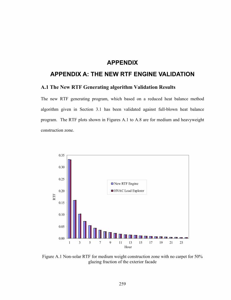
259
APPENDIX
APPENDIX A: THE NEW RTF ENGINE VALIDATION
A.1 The New RTF Generating algorithm Validation Results
The new RTF generating program, which based on a reduced heat balance method
algorithm given in Section 3.1 has been validated against full-blown heat balance
program. The RTF plots shown in Figures A.1 to A.8 are for medium and heavyweight
construction zone.
0.00
0.05
0.10
0.15
0.20
0.25
0.30
0.35
1 3 5 7 9 11 13 15 17 19 21 23Hour
RTF
New RTF Engine
HVAC Load Explorer
Figure A.1 Non-solar RTF for medium weight construction zone with no carpet for 50%
glazing fraction of the exterior facade
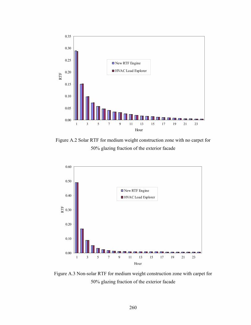
260
0.00
0.05
0.10
0.15
0.20
0.25
0.30
0.35
1 3 5 7 9 11 13 15 17 19 21 23
Hour
RTF
New RTF Engine
HVAC Load Explorer
Figure A.2 Solar RTF for medium weight construction zone with no carpet for
50% glazing fraction of the exterior facade
0.00
0.10
0.20
0.30
0.40
0.50
0.60
1 3 5 7 9 11 13 15 17 19 21 23
Hour
RTF
New RTF Engine
HVAC Load Explorer
Figure A.3 Non-solar RTF for medium weight construction zone with carpet for
50% glazing fraction of the exterior facade
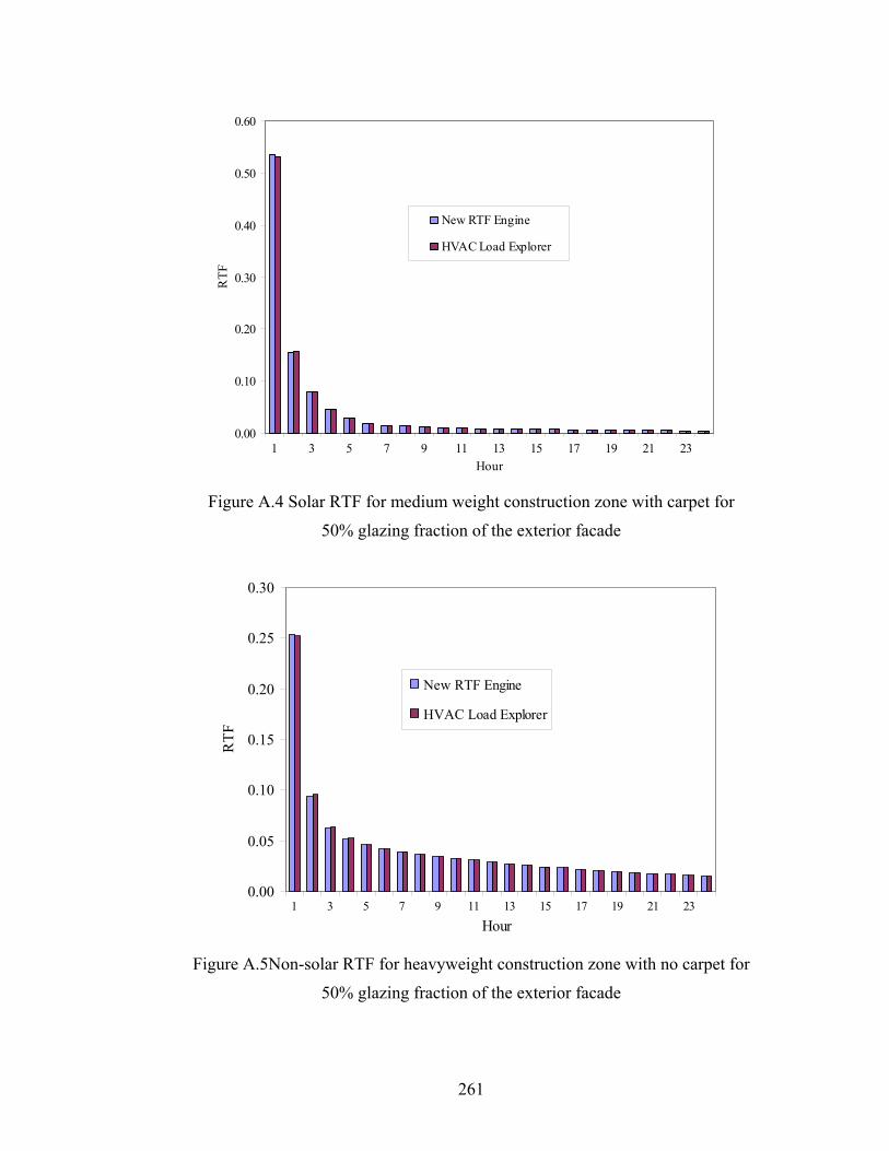
261
0.00
0.10
0.20
0.30
0.40
0.50
0.60
1 3 5 7 9 11 13 15 17 19 21 23Hour
RTF
New RTF Engine
HVAC Load Explorer
Figure A.4 Solar RTF for medium weight construction zone with carpet for
50% glazing fraction of the exterior facade
0.00
0.05
0.10
0.15
0.20
0.25
0.30
1 3 5 7 9 11 13 15 17 19 21 23
Hour
RTF
New RTF Engine
HVAC Load Explorer
Figure A.5Non-solar RTF for heavyweight construction zone with no carpet for
50% glazing fraction of the exterior facade
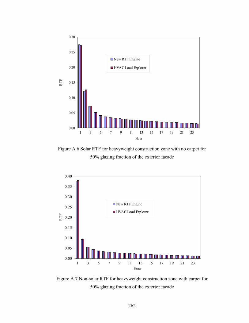
262
0.00
0.05
0.10
0.15
0.20
0.25
0.30
1 3 5 7 9 11 13 15 17 19 21 23Hour
RTF
New RTF Engine
HVAC Load Explorer
Figure A.6 Solar RTF for heavyweight construction zone with no carpet for
50% glazing fraction of the exterior facade
0.00
0.05
0.10
0.15
0.20
0.25
0.30
0.35
0.40
1 3 5 7 9 11 13 15 17 19 21 23Hour
RTF
New RTF Engine
HVAC Load Explorer
Figure A.7 Non-solar RTF for heavyweight construction zone with carpet for
50% glazing fraction of the exterior facade
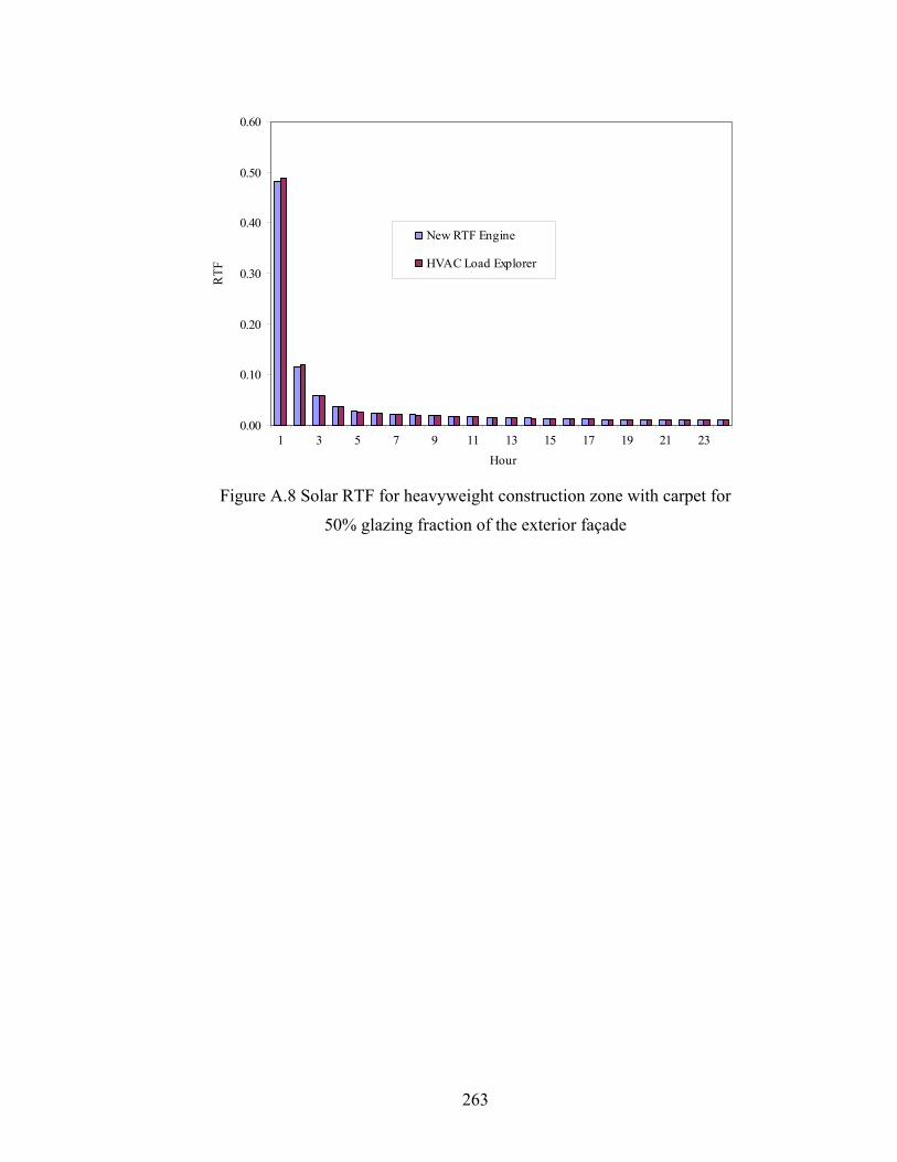
263
0.00
0.10
0.20
0.30
0.40
0.50
0.60
1 3 5 7 9 11 13 15 17 19 21 23Hour
RTF
New RTF Engine
HVAC Load Explorer
Figure A.8 Solar RTF for heavyweight construction zone with carpet for
50% glazing fraction of the exterior façade
264
APPENDIX B: 1D FINITE VOLUME METHOD PERIODIC RESPONSE FACTOR GENERATION
B.1 Derivation 1D Finite Volume Numerical Model
Heat conduction in building envelopes is commonly represented by one-dimensional
transient heat conduction equation which is expressed as follows:
( )
=
dxdk
dxd
dtcd φφρ (B.1)
Where
ρc = is the product of density and specific heat, J/m3⋅°C (Btu/ft3⋅°F)
k = is the thermal conductivity of the material, W/m⋅°C (Btu-in/ft2⋅°F)
φ = is the temperature, °C (°F)
t = is the time, s (sec)
x = is the thickness in the direction of the heat flow path, m(in)
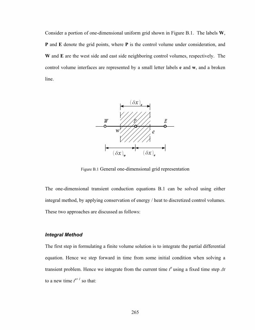
265
Consider a portion of one-dimensional uniform grid shown in Figure B.1. The labels W,
P and E denote the grid points, where P is the control volume under consideration, and
W and E are the west side and east side neighboring control volumes, respectively. The
control volume interfaces are represented by a small letter labels e and w, and a broken
line.
Figure B.1 General one-dimensional grid representation
The one-dimensional transient conduction equations B.1 can be solved using either
integral method, by applying conservation of energy / heat to discretized control volumes.
These two approaches are discussed as follows:
Integral Method
The first step in formulating a finite volume solution is to integrate the partial differential
equation. Hence we step forward in time from some initial condition when solving a
transient problem. Hence we integrate from the current time tn using a fixed time step ∆t
to a new time tn+1 so that:
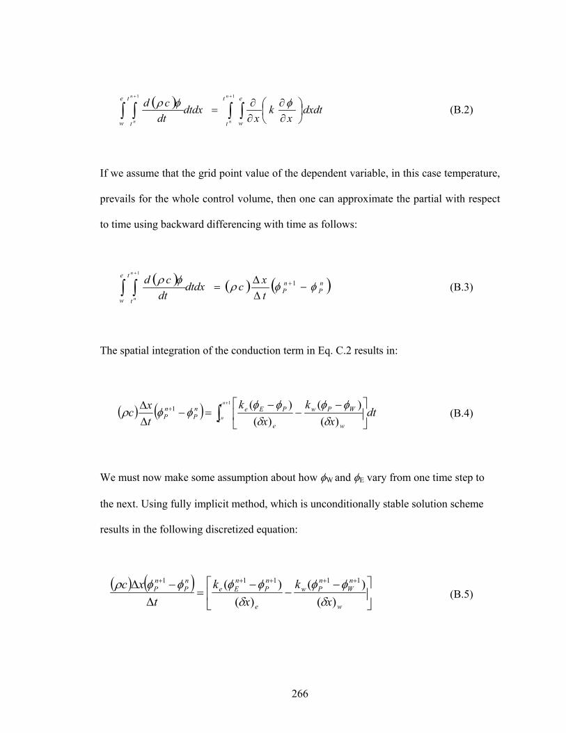
266
( ) dxdtx
kx
dtdxdt
cdn
n
n
n
t
t
e
w
e
w
t
t
∂∂
∂∂
= ∫ ∫∫ ∫++
φφρ11
(B.2)
If we assume that the grid point value of the dependent variable, in this case temperature,
prevails for the whole control volume, then one can approximate the partial with respect
to time using backward differencing with time as follows:
( ) ( ) ( )nP
nP
e
w
t
t txcdtdx
dtcd
n
n
φφρφρ−
∆∆
= +∫ ∫+
1
1
(B.3)
The spatial integration of the conduction term in Eq. C.2 results in:
( ) ( ) dtx
kx
ktxc
n
n
t
tw
WPw
e
PEenP
nP ∫
+
−−
−=−
∆∆ +
1
)()(
)()(1
δφφ
δφφ
φφρ (B.4)
We must now make some assumption about how φW and φE vary from one time step to
the next. Using fully implicit method, which is unconditionally stable solution scheme
results in the following discretized equation:
( ) ( )
−−
−=
∆−∆ +++++
w
nW
nPw
e
nP
nEe
nP
nP
xk
xk
txc
)()(
)()( 11111
δφφ
δφφφφρ
(B.5)
267
It can be seen that the temporal term is equivalent to first-order backwards differencing in
time. The discretized equation can then be said to be first-order accurate in time and
second-order accurate in space.
Energy Conservation Method
This method is basically the fundamental concept used in deriving the differential form of
the heat equation given in Eq B.1. Applying conservation of energy around the control
volume P shown in Figure B.1. Ignoring potential energy, kinetic energy and in the
absence of internal heat generation, the net inflow of heat into the control volume P is
equal to the rate of change of the internal of energy of the control volume and is given by:
EqAqA eeww&&& ∆=− '''' (B.6)
The heat flux terms crossing the control volume surfaces using the Fourier laws of heat
conduction are given by:
e
PEee
w
WPww
xkq
xkq
)(
)(
''
''
δφφ
δφφ
−−=
−−=
&
&
(B.7)
Similarly the rate of change of the internal energy of the control volume is given by:
tcVE PP
∆−
=∆0
)( φφρδ& (B.8)
268
Substituting Eq. B.7 and Eq B.8 into Eq. B.6 yields:
tcV
xk
xkA PP
e
PEe
w
WPww ∆
−=
−+
−−
0
)()()(
φφρδδ
φφδ
φφ (B.9)
For equal area in the direction of heat conduction Eq. B.9 reduces to:
w
PWw
e
EPe
PP
xk
xk
tcx
)()()(
0
δφφ
δφφφφρδ −
−−
=∆− (B.10)
Eq. B.10 is identical to Eq. B.5 derived using the integral method. The solution technique
adapted here for either these equations require further manipulations to represent the
equation in terms of constant coefficient and the nodal temperatures in a form convenient
for solving. This is discussed in the following section.
Collecting together terms to form an equation in terms of the nodal values of the
dependent variable forms:
caaa EEWWPP ++= φφφ (B.11)
Where,
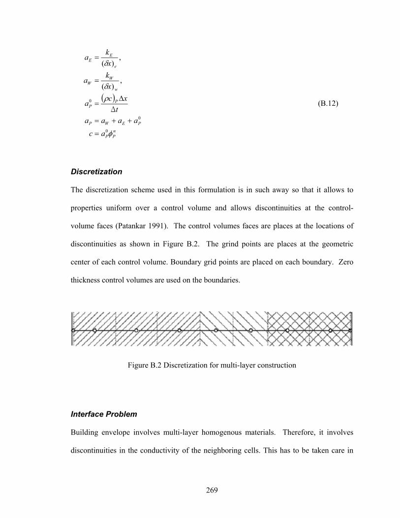
269
( )
nPP
PEWP
PP
w
WW
e
EE
ac
aaaat
xca
xka
xka
φ
ρδ
δ
0
0
0
,)(
,)(
=
++=
∆=
=
=
Δ (B.12)
Discretization
The discretization scheme used in this formulation is in such away so that it allows to
properties uniform over a control volume and allows discontinuities at the control-
volume faces (Patankar 1991). The control volumes faces are places at the locations of
discontinuities as shown in Figure B.2. The grind points are places at the geometric
center of each control volume. Boundary grid points are placed on each boundary. Zero
thickness control volumes are used on the boundaries.
Figure B.2 Discretization for multi-layer construction
Interface Problem
Building envelope involves multi-layer homogenous materials. Therefore, it involves
discontinuities in the conductivity of the neighboring cells. This has to be taken care in
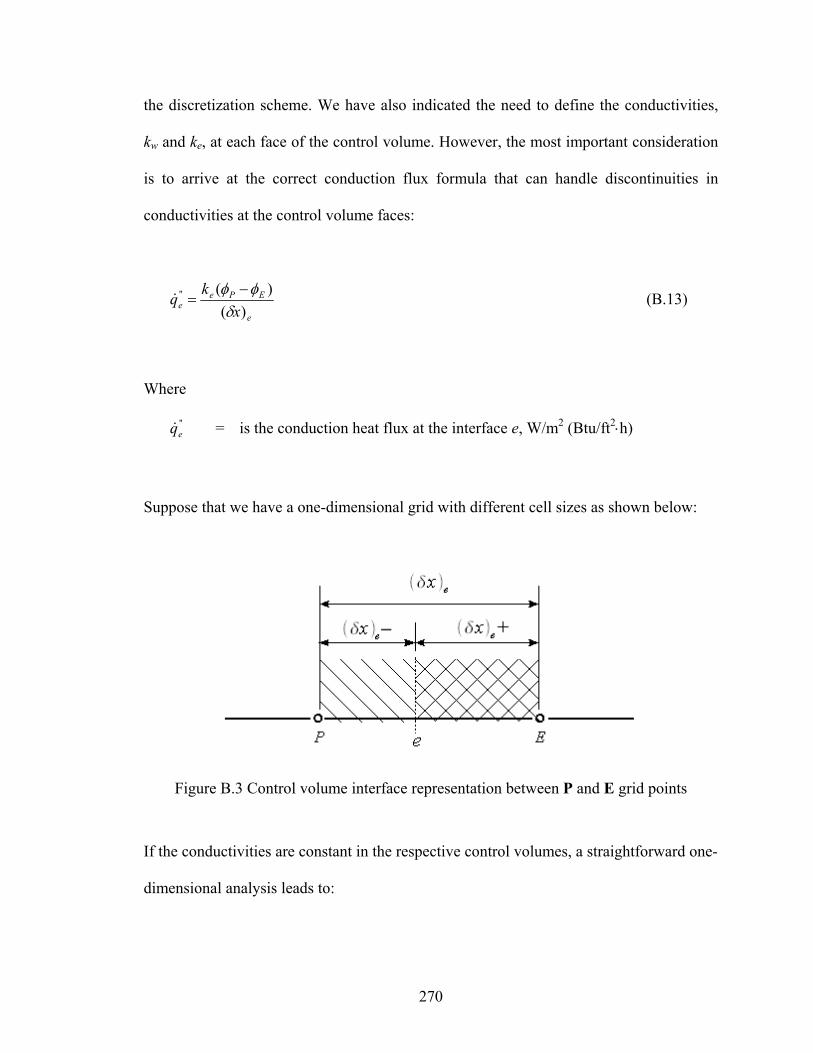
270
the discretization scheme. We have also indicated the need to define the conductivities,
kw and ke, at each face of the control volume. However, the most important consideration
is to arrive at the correct conduction flux formula that can handle discontinuities in
conductivities at the control volume faces:
e
EPee x
kq)(
)(''
δφφ −
=& (B.13)
Where
''eq& = is the conduction heat flux at the interface e, W/m2 (Btu/ft2⋅h)
Suppose that we have a one-dimensional grid with different cell sizes as shown below:
Figure B.3 Control volume interface representation between P and E grid points
If the conductivities are constant in the respective control volumes, a straightforward one-
dimensional analysis leads to:
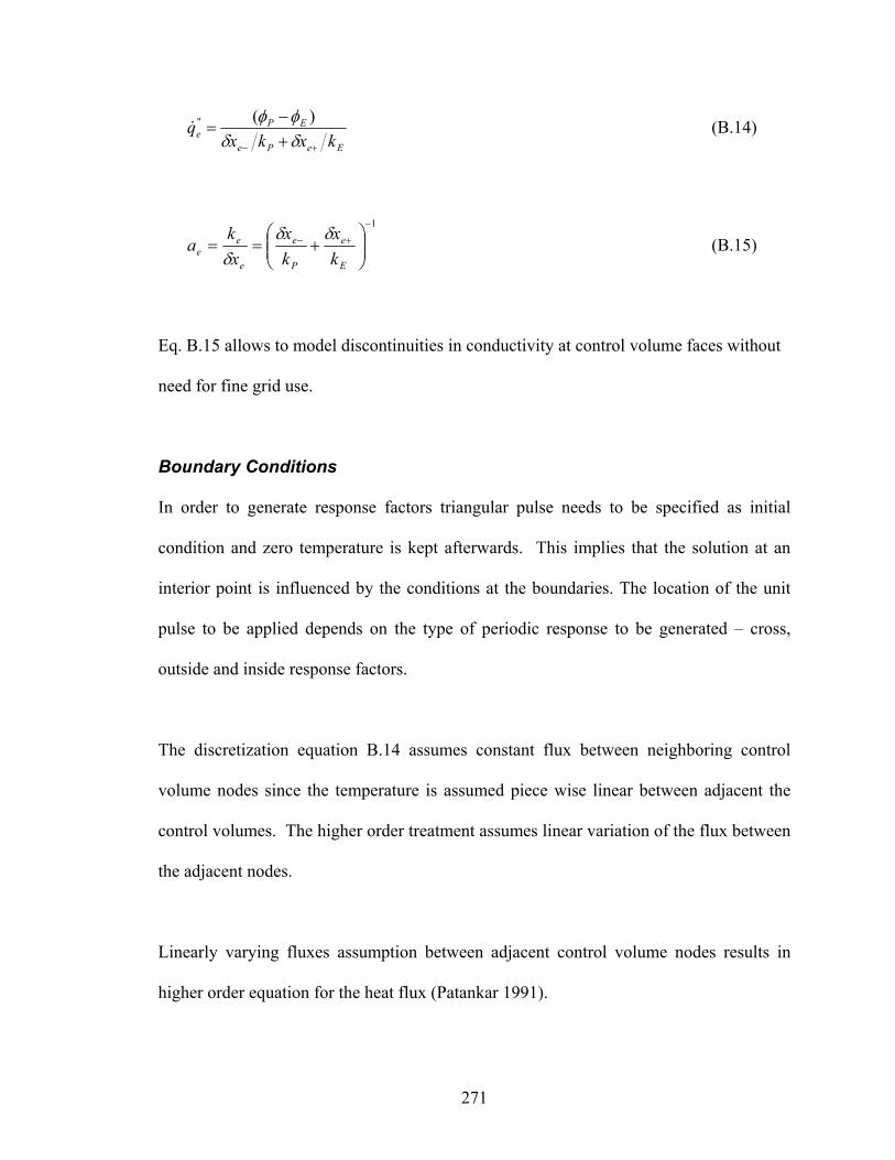
271
EePe
EPe kxkx
q+− +
−=
δδφφ )(''& (B.14)
1−
+−
+==
E
e
P
e
e
ee k
xkx
xk
aδδ
δ (B.15)
Eq. B.15 allows to model discontinuities in conductivity at control volume faces without
need for fine grid use.
Boundary Conditions
In order to generate response factors triangular pulse needs to be specified as initial
condition and zero temperature is kept afterwards. This implies that the solution at an
interior point is influenced by the conditions at the boundaries. The location of the unit
pulse to be applied depends on the type of periodic response to be generated – cross,
outside and inside response factors.
The discretization equation B.14 assumes constant flux between neighboring control
volume nodes since the temperature is assumed piece wise linear between adjacent the
control volumes. The higher order treatment assumes linear variation of the flux between
the adjacent nodes.
Linearly varying fluxes assumption between adjacent control volume nodes results in
higher order equation for the heat flux (Patankar 1991).

272
Figure B.4 Control volume at the left boundary and linear varying flux representation
Applying this assumption to the boundary nodes shown in Figure B.4 yields:
( ) 3212
22 3
134 q
xk
q −
−
=
−
φφδ
(B.16)
3322
323
)(kxkx
q−+ +
−=
δδφφ
(B.17)
The coefficient for the boundary nodes due to the higher order treatment is given by:
1
3
3
2
22
2
22
34
34
−
−+
+=
=
kx
kxa
xkb
δδ
δ (B.18)
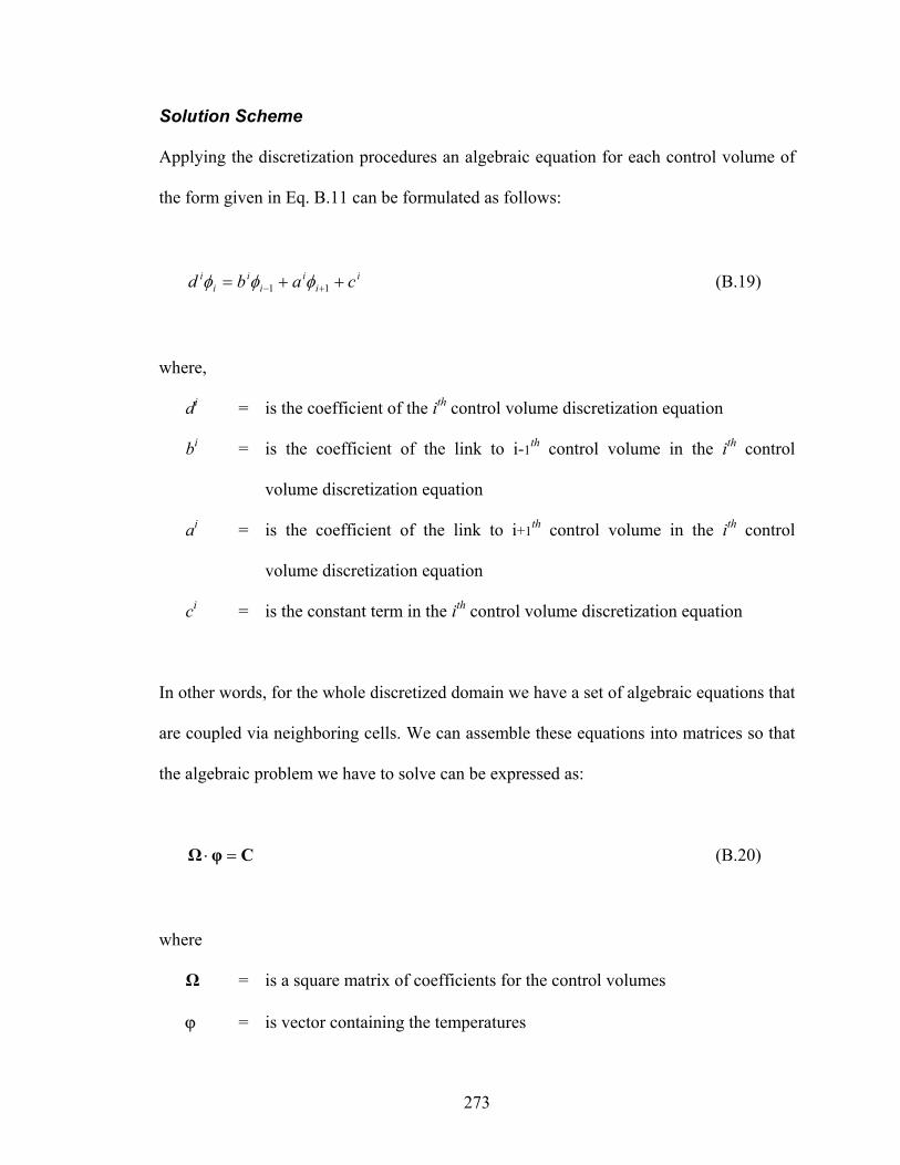
273
Solution Scheme
Applying the discretization procedures an algebraic equation for each control volume of
the form given in Eq. B.11 can be formulated as follows:
ii
ii
ii
i cabd ++= +− 11 φφφ (B.19)
where,
di = is the coefficient of the ith control volume discretization equation
bi = is the coefficient of the link to i-1th control volume in the ith control
volume discretization equation
ai = is the coefficient of the link to i+1th control volume in the ith control
volume discretization equation
ci = is the constant term in the ith control volume discretization equation
In other words, for the whole discretized domain we have a set of algebraic equations that
are coupled via neighboring cells. We can assemble these equations into matrices so that
the algebraic problem we have to solve can be expressed as:
CφΩ =⋅ (B.20)
where
Ω = is a square matrix of coefficients for the control volumes
ϕ = is vector containing the temperatures

274
C = is vector containing the right hand side constant coefficients
For this linear partial differential equation the solution of the matrix formulation can be
determined by using a suitable linear equation solver. The method we apply to solve Eq
B.16 depends partly on the properties of the Ω matrix coefficients. The matrix equation
for a one-dimensional conduction with nine nodes, when fully expanded, looks like:
=
8
7
6
5
4
3
2
8
7
6
5
4
3
2
88
777
666
555
444
333
22
000000000
000000000000000000000
ccccccc
dbadb
adbadb
adbadb
ad
φφφφφφφ
(B.21)
A notable property of this matrix is its tri-diagonal structure. This allows the use of a very
efficient algorithm known as the Thomas Algorithm or the Tri-Diagonal Matrix
Algorithm (TDMA). This is a type of Gauss elimination and can be explained as follows.
We can express the equations that make up the matrix as:
ii
ii
ii
i cadb =++ +− 11 φφφ (B.22)
Where i is the control volume counter in the range from 2 to 8, and we note that b2 = 0
and a8 = 0. The discretization algebraic equation Eq B.15 for the boundary nodes can be
written as follows:
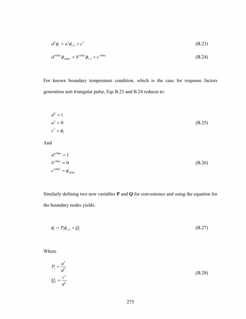
275
11
11
1 cad i += +φφ (B.23)
nMaxi
nMaxnMax
nMax cbd += −1φφ (B.24)
For known boundary temperature condition, which is the case for response factors
generation unit triangular pulse, Eqs B.23 and B.24 reduces to:
11
1
1
01
φ=
=
=
cad
(B.25)
And
nMaxnMax
nMax
nMax
cbd
φ=
=
=
01
(B.26)
Similarly defining two new variables P and Q for convenience and using the equation for
the boundary nodes yields:
1111 QP i += +φφ (B.27)
Where
1
1
1
1
1
1
dcQ
daP
=
= (B.28)
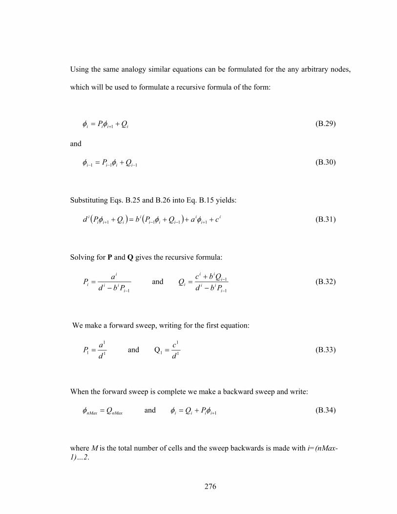
276
Using the same analogy similar equations can be formulated for the any arbitrary nodes,
which will be used to formulate a recursive formula of the form:
iiii QP += +1φφ (B.29)
and
111 −−− += iiii QP φφ (B.30)
Substituting Eqs. B.25 and B.26 into Eq. B.15 yields:
( ) ( ) ii
iiii
iiii
i caQPbQPd +++=+ +−−+ 1111 φφφ (B.31)
Solving for P and Q gives the recursive formula:
1
1
1
and −
−
− −+
=−
=i
iii
ii
ii
ii
i
i PbdQbc
QPbd
aP (B.32)
We make a forward sweep, writing for the first equation:
Q and 1
1
11
1
1 dc
daP == (B.33)
When the forward sweep is complete we make a backward sweep and write:
1 and ++== iiiinMaxnMax PQQ φφφ (B.34)
where M is the total number of cells and the sweep backwards is made with i=(nMax-1)…2.
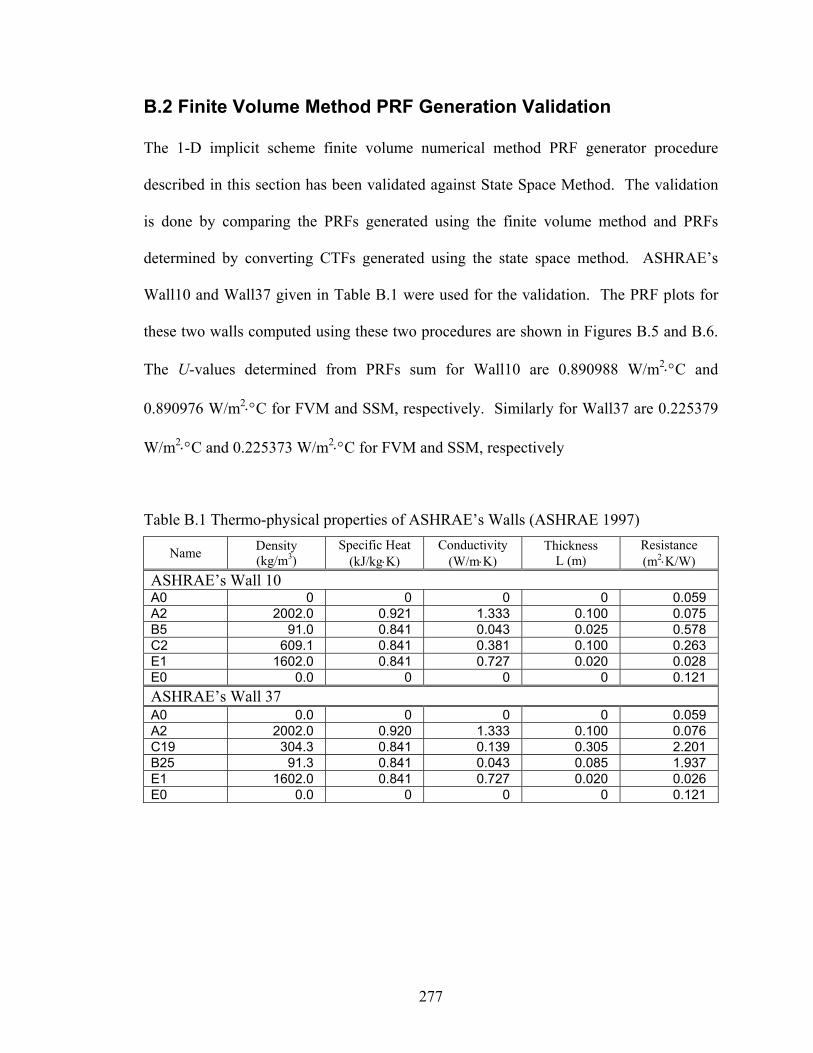
277
B.2 Finite Volume Method PRF Generation Validation
The 1-D implicit scheme finite volume numerical method PRF generator procedure
described in this section has been validated against State Space Method. The validation
is done by comparing the PRFs generated using the finite volume method and PRFs
determined by converting CTFs generated using the state space method. ASHRAE’s
Wall10 and Wall37 given in Table B.1 were used for the validation. The PRF plots for
these two walls computed using these two procedures are shown in Figures B.5 and B.6.
The U-values determined from PRFs sum for Wall10 are 0.890988 W/m2⋅°C and
0.890976 W/m2⋅°C for FVM and SSM, respectively. Similarly for Wall37 are 0.225379
W/m2⋅°C and 0.225373 W/m2⋅°C for FVM and SSM, respectively
Table B.1 Thermo-physical properties of ASHRAE’s Walls (ASHRAE 1997)
Name Density (kg/m3)
Specific Heat (kJ/kg⋅K)
Conductivity (W/m⋅K)
Thickness L (m)
Resistance (m2⋅K/W)
ASHRAE’s Wall 10 A0 0 0 0 0 0.059 A2 2002.0 0.921 1.333 0.100 0.075 B5 91.0 0.841 0.043 0.025 0.578 C2 609.1 0.841 0.381 0.100 0.263 E1 1602.0 0.841 0.727 0.020 0.028 E0 0.0 0 0 0 0.121 ASHRAE’s Wall 37 A0 0.0 0 0 0 0.059 A2 2002.0 0.920 1.333 0.100 0.076 C19 304.3 0.841 0.139 0.305 2.201 B25 91.3 0.841 0.043 0.085 1.937 E1 1602.0 0.841 0.727 0.020 0.026 E0 0.0 0 0 0 0.121
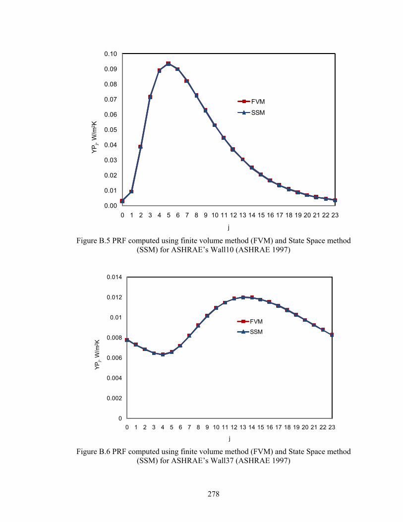
278
0.00
0.01
0.02
0.03
0.04
0.05
0.06
0.07
0.08
0.09
0.10
0 1 2 3 4 5 6 7 8 9 10 11 12 13 14 15 16 17 18 19 20 21 22 23
YPj,
W/m
2 K
j
FVM
SSM
Figure B.5 PRF computed using finite volume method (FVM) and State Space method
(SSM) for ASHRAE’s Wall10 (ASHRAE 1997)
0
0.002
0.004
0.006
0.008
0.01
0.012
0.014
0 1 2 3 4 5 6 7 8 9 10 11 12 13 14 15 16 17 18 19 20 21 22 23
YPj,
W/m
2 K
j
FVM
SSM
Figure B.6 PRF computed using finite volume method (FVM) and State Space method (SSM) for ASHRAE’s Wall37 (ASHRAE 1997)
279
APPENDIX – C: RTSM IMPLEMENTATION IN OTHER COMPUTING ENVIRONMENTS
C.1 RTF Generator Implementation in SCILAB //RTF Generation: reads periodic response factors and surface area from a text file and sets up // the zone heat balance matrix and solves for the Radiant Time Factors. N = 12; YZP=file('open','C:\SCILAB\PRF.text','old'); SA=file('open','AREA.DAT','last','old'); // opens test file PRFD=read(YZP,288,2); // reads response factors file A=read(SA,1,12); // reads surface areas from file file('close',YZP); Qgain=1000.; for j=1:N; for i=1:24; YP(i,j)=PRFD((j-1)*24+i,1); ZP(i,j)=PRFD((j-1)*24+i,2);end;end PRF=file('open','YZPRF.text','unknown'); write(PRF,PRFD,'(2(f15.10,2x))'); file('close',PRF); // creat the system matrix for j=1:N; OMEGA(j,1,1)=ZP(1,j)-YP(1,j); for k=2:24;kk=24-k+2;OMEGA(j,1,k)=ZP(kk,j)-YP(kk,j);end; for i=2:24; for k=1:24; kk=k+1; if kk > 24 then, kk=kk-24; else, end; OMEGA(j,i,kk)=OMEGA(j,i-1,k);end;end; end // define surface areas in the zone em=[0.9 0.9 0.9 0.9 0.9 0.9 0.9 0.9 0.9 0.9 0.9 0.9]; exec('C:\SCILAB\RTFFUNCTIONS.SCI',-1); exists('AreaFraction'); exists('InsideRadiationCoef'); exists('MeanRadiantTemperature'); exists('Response'); AF=AreaFraction(A,N,em,N); for j=1:N; MRTVF(j)=1./(1.-A(j)/sum(A));end;

280
Iter=0; while Iter < 10, for i=1:N; A_MRTVF_Product=0.0d0; for j=1:N; A_MRTVF_Product=A_MRTVF_Product+A(j)*MRTVF(j); end; MRTVF(i)=1./(1.-A(i)*MRTVF(i)/A_MRTVF_Product);end; Iter=Iter+1;, else, end; // Iteration Loop // Sigma=5.67E-8; // Initialize the hourly values of the radiation coefficient for i=1:24; // number of hours for j=1:N; // number of surfaces hradbase(j,i) = 4*Sigma*(27+273.15)**3 / (1/MRTVF(j)+(1-em(j)))/em(j);end; // surface Loop end // Hour loop for i=1:24;TROOM(i)=24.0;TMRT(i)=24.0;end for j=1:N; for i=1:24; TsIn(j,i)=TROOM(i);hrad(j,i)=hradbase(j,i);end;end for j=1:N;hcIn(j)=4.68;end hcIn(5)=1.25; hcIn(6)=4.37; // calculate mean radiant temperatures for Mode=1:2; // Mode 1 for non solar RTF and Mode=2 solar RTF if Mode==1 then, for i=1:24; if i==1 then LWRadIntGain = Qgain; else LWRadIntGain = 0.0d0; end for j=1:N; Distribution(j) = AF(j); if A(j) == 0 then RadPulseDist(j,i) = 0.0; else RadPulseDist(j,i) = LWRadIntGain*Distribution(j)/A(j); end, end;end else, for i=1:24; if i==1 then LWRadIntGain = Qgain; else LWRadIntGain = 0.0d0; end for j=1:N; Distribution(j)=0.0; if j==6 then Distribution(j)=0.5; elseif j==7 Distribution(j)=0.5; else end if A(j) == 0 then RadPulseDist(j,i) = 0.0; else RadPulseDist(j,i) = LWRadIntGain*Distribution(j)/A(j);end, end;end end // iteration starts here Iter=0; while Iter < 25 then // iteration for convergence for j=1:N; for i=1:24; C(i)=hcIn(j)*TROOM(i)+hrad(j,i)*TMRT(i)+RadPulseDist(j,i);end // generate the left hand side system matrix B for i=1:24; for k=1:24; B(i,k) = OMEGA(j,i,k);

281
if i==k then B(i,k) = hcIn(j) + hrad(j,i) + B(i,k); else, end end; end BM=file('open','MATRIX.text','unknown'); write(BM,B,'(24(f10.6,1x))'); file('close',BM); // Calculates the surface temperature by matrix inversion and multiplication BInv = inv(B); Ts = BInv*C; for k=1:24; TsIn(j,k)=Ts(k);end end // end of surface loop j hrad=InsideRadiationCoef(TsIn,TMRT); TMRT=MeanRadiantTemperature(A,TsIn,hrad); hrad=InsideRadiationCoef(TsIn,TMRT); Iter=Iter+1; else, TsIn; end; // end if while loop if(Mode==1) then, [NONSOLARRTF]=Response(A,hcIn,TsIn); RTFSUM=sum(NONSOLARRTF) else, [SOLARRTF]=Response(A,hcIn,TsIn); RTFSUM=sum(SOLARRTF) end end; // end of pulse distribution. NONSOLARRTF SOLARRTF function AF=AreaFraction(A,N,em,N) AF=A.*em/(sum(A.*em)) endfunction function TMRT = MeanRadiantTemperature(A,TsIn,hrad) [nS nH]=size(TsIn); for i=1:nH; A_hrad_Temperature(i)=0.0; A_hrad_Product(i)=0.0; for j=1:nS; A_hrad_Product(i)=A_hrad_Product(i)+A(j)*hrad(j,i); A_hrad_Temperature(i)=A_hrad_Temperature(i)+A(j)*hrad(j,i)*TsIn(j,i);end; TMRT(i) = A_hrad_Temperature(i)/A_hrad_Product(i);end endfunction function hrad =InsideRadiationCoef(TsIn,TMRT) [nS nH]=size(TsIn); for i=1:nH;for j=1:nS; hrad(j,i)=(0.865+TsIn(j,i)/200)*hradbase(j,i);end;end; for i=1:nH;for j=1:nS; hrad(j,i)=(0.865 + TMRT(i)/200)*hrad(j,i);end;end endfunction // compute the zone response function RTF=Response(A,hcIn,TsIn) [nS nH]=size(TsIn); for i=1:nH; RTF(i)=0.0; for j=1:nS;
282
RTF(i)=RTF(i)+A(j)*hcIn(j)*(TsIn(j,i)-TROOM(j))/Qgain;end; end endfunction
C.2 RTSM Implementation in VBA
The RTSM cooling load calculation procedure has been implemented as a spreadsheets
application using VBA programming and worksheet functions. The CTS and RTF were
generated using three different approaches:
Compiled FORTRAN DLL
VBA sub-program with variable radiation coefficients
VBA sub-program with constant radiation coefficients
Three thermal zones from ASHRAE head quarter building in Atlanta, Georgia were used
as test zones. The hourly cooling loads were calculated for the twelve design days for
each zone and the annual peak design day cooling loads were extracted. The hourly
design day cooling load for three zones and the three different approaches are shown in
Figure C.1 to C.3. The hourly cooling load show very good match. The hourly cooling
load error by using constant radiation coefficients was less than 0.02 Btu/h⋅ft2.
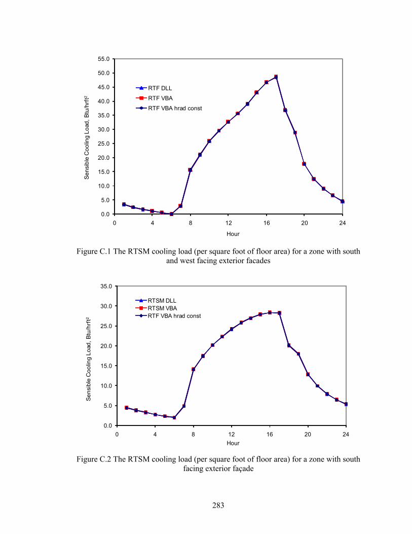
283
0.0
5.0
10.0
15.0
20.0
25.0
30.0
35.0
40.0
45.0
50.0
55.0
0 4 8 12 16 20 24
Sens
ible
Coo
ling
Load
, Btu
/hrf
t2
Hour
RTF DLL
RTF VBA
RTF VBA hrad const
Figure C.1 The RTSM cooling load (per square foot of floor area) for a zone with south
and west facing exterior facades
0.0
5.0
10.0
15.0
20.0
25.0
30.0
35.0
0 4 8 12 16 20 24
Sens
ible
Coo
ling
Load
, Btu
/hrf
t2
Hour
RTSM DLLRTSM VBARTF VBA hrad const
Figure C.2 The RTSM cooling load (per square foot of floor area) for a zone with south
facing exterior façade
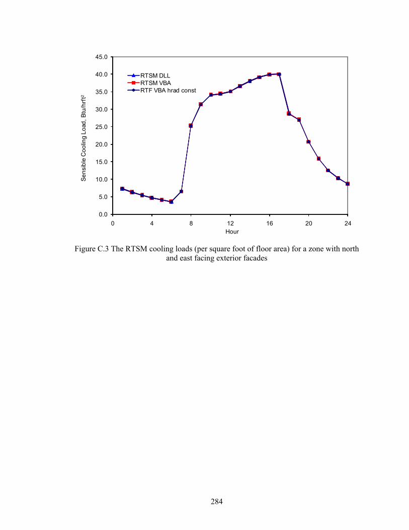
284
0.0
5.0
10.0
15.0
20.0
25.0
30.0
35.0
40.0
45.0
0 4 8 12 16 20 24
Sens
ible
Coo
ling
Load
, Btu
/hrf
t2
Hour
RTSM DLLRTSM VBARTF VBA hrad const
Figure C.3 The RTSM cooling loads (per square foot of floor area) for a zone with north
and east facing exterior facades
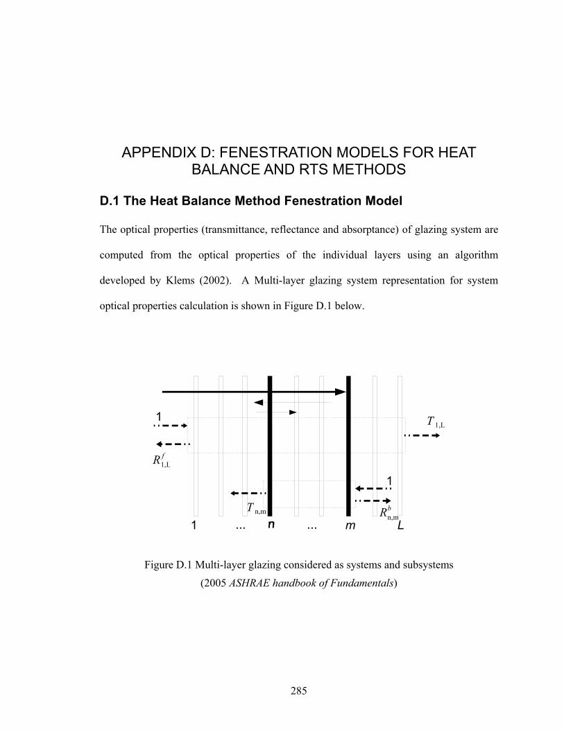
285
APPENDIX D: FENESTRATION MODELS FOR HEAT BALANCE AND RTS METHODS
D.1 The Heat Balance Method Fenestration Model
The optical properties (transmittance, reflectance and absorptance) of glazing system are
computed from the optical properties of the individual layers using an algorithm
developed by Klems (2002). A Multi-layer glazing system representation for system
optical properties calculation is shown in Figure D.1 below.
n mn L1Rn,m
b
R1,Lf
T n,m
T 1,L1
... ...
1
Figure D.1 Multi-layer glazing considered as systems and subsystems
(2005 ASHRAE handbook of Fundamentals)
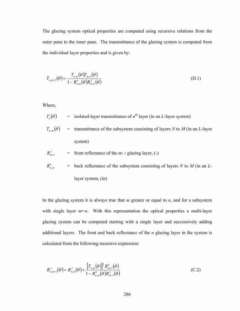
286
The glazing system optical properties are computed using recursive relations from the
outer pane to the inner pane. The transmittance of the glazing system is computed from
the individual layer properties and is given by:
( ) ( ) ( )( ) ( )θθ
θθθ f
mb
mn
mmnmn RR
TTT
1,
1,1, 1 +
++ −
= (D.1)
Where,
( )θnT = isolated-layer transmittance of nth layer (in an L-layer system)
( )θmnT , = transmittance of the subsystem consisting of layers N to M (in an L-layer
system)
fmR 1+ = front reflectance of the m+1 glazing layer, (-)
bmnR , = back reflectance of the subsystem consisting of layers N to M (in an L-
layer system, (in)
In the glazing system it is always true that m greater or equal to n, and for a subsystem
with single layer m=n. With this representation the optical properties a multi-layer
glazing system can be computed starting with a single layer and successively adding
additional layers. The front and back reflectance of the n glazing layer in the system is
calculated from the following recursive expression:
( ) ( ) ( )[ ] ( )( ) ( )θθ
θθθθ f
mb
mn
bmmnf
mnf
mn RRRT
RR1,
12
,,1, 1 +
++ −
+= (C.2)
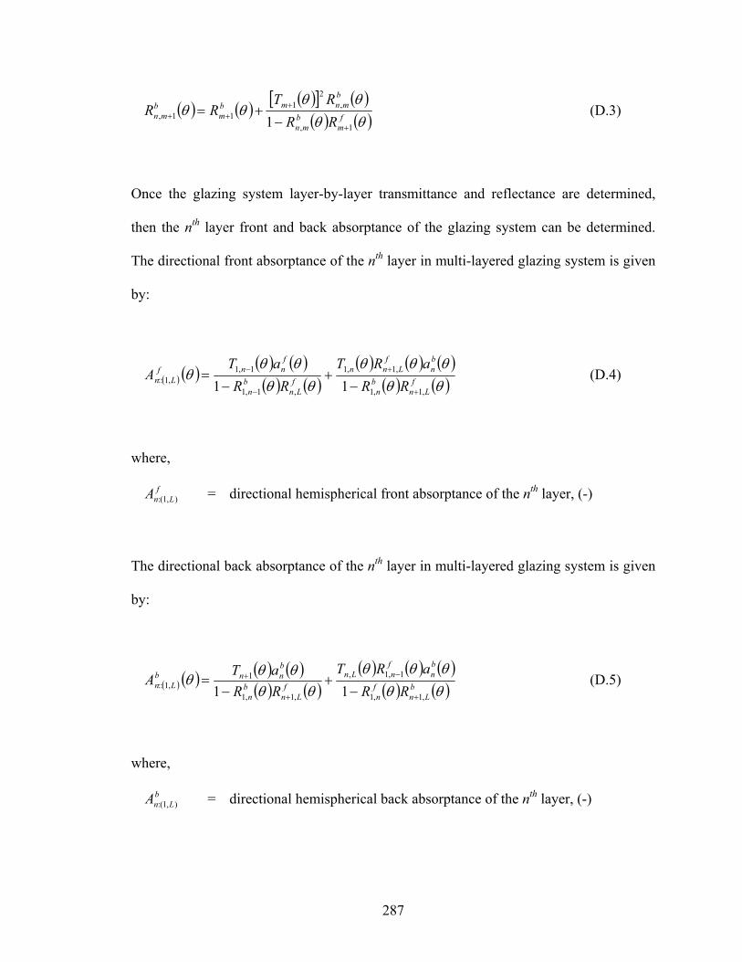
287
( ) ( ) ( )[ ] ( )( ) ( )θθ
θθθθ f
mb
mn
bmnmb
mb
mn RRRT
RR1,
,2
111, 1 +
+++ −
+= (D.3)
Once the glazing system layer-by-layer transmittance and reflectance are determined,
then the nth layer front and back absorptance of the glazing system can be determined.
The directional front absorptance of the nth layer in multi-layered glazing system is given
by:
( ) ( ) ( ) ( )( ) ( )
( ) ( ) ( )( ) ( )θθ
θθθθθ
θθθ f
Lnb
n
bn
fLnn
fLn
bn
fnnf
Ln RRaRT
RRaT
A,1,1
,1,1
,1,1
1,1,1:: 11 +
+
−
−
−+
−= (D.4)
where,
fLnA ),1(: = directional hemispherical front absorptance of the nth layer, (-)
The directional back absorptance of the nth layer in multi-layered glazing system is given
by:
( ) ( ) ( ) ( )( ) ( )
( ) ( ) ( )( ) ( )θθ
θθθθθ
θθθ b
Lnfn
bn
fnLn
fLn
bn
bnnb
Ln RRaRT
RRaT
A,1,1
1,1,
,1,1
1,1:: 11 +
−
+
+
−+
−= (D.5)
where,
bLnA ),1(: = directional hemispherical back absorptance of the nth layer, (-)
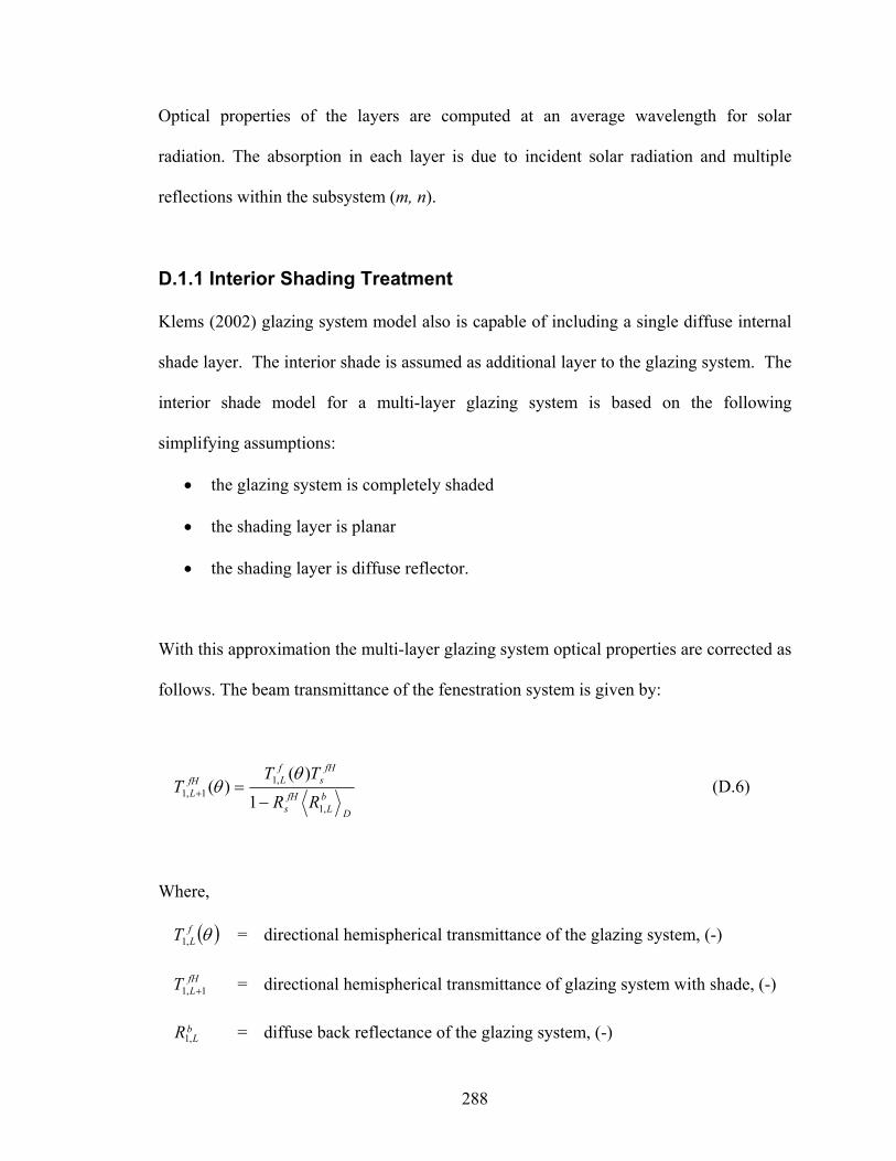
288
Optical properties of the layers are computed at an average wavelength for solar
radiation. The absorption in each layer is due to incident solar radiation and multiple
reflections within the subsystem (m, n).
D.1.1 Interior Shading Treatment
Klems (2002) glazing system model also is capable of including a single diffuse internal
shade layer. The interior shade is assumed as additional layer to the glazing system. The
interior shade model for a multi-layer glazing system is based on the following
simplifying assumptions:
• the glazing system is completely shaded
• the shading layer is planar
• the shading layer is diffuse reflector.
With this approximation the multi-layer glazing system optical properties are corrected as
follows. The beam transmittance of the fenestration system is given by:
D
bL
fHs
fHs
fLfH
L RRTT
T,1
,11,1 1
)()(
−=+
θθ (D.6)
Where,
( )θfLT ,1 = directional hemispherical transmittance of the glazing system, (-)
fHLT 1,1 + = directional hemispherical transmittance of glazing system with shade, (-)
bLR ,1 = diffuse back reflectance of the glazing system, (-)
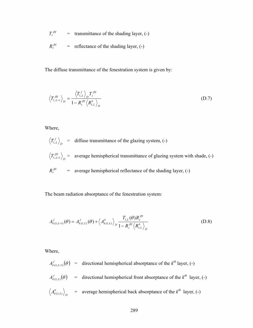
289
fHsT = transmittance of the shading layer, (-)
fHsR = reflectance of the shading layer, (-)
The diffuse transmittance of the fenestration system is given by:
D
bL
fHs
fHsD
fL
D
fHL RR
TTT
,1
,11,1 1−
=+ (D.7)
Where,
D
fLT ,1 = diffuse transmittance of the glazing system, (-)
D
fHLT 1,1 + = average hemispherical transmittance of glazing system with shade, (-)
fHsR = average hemispherical reflectance of the shading layer, (-)
The beam radiation absorptance of the fenestration system:
D
bL
fHs
fHsL
D
bLk
fLk
fLk RR
RTAAA
,1
,1),1(:),1(:)1,1(: 1
)()()(
−+=+
θθθ (D.8)
Where,
( )θfLkA )1,1(: + = directional hemispherical absorptance of the kth layer, (-)
( )θfLkA ),1(: = directional hemispherical front absorptance of the kth layer, (-)
D
bLkA ),1(: = average hemispherical back absorptance of the kth layer, (-)
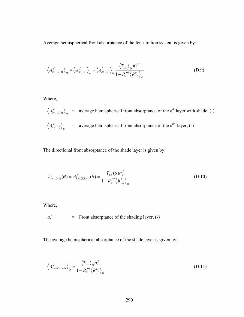
290
Average hemispherical front absorptance of the fenestration system is given by:
D
bL
fHs
fHsDL
D
bLkD
fLkD
fLk RR
RTAAA
,1
,1),1(:),1(:)1,1(: 1−
+=+ (D.9)
Where,
D
fLkA )1,1(: + = average hemispherical front absorptance of the kth layer with shade, (-)
D
fLkA ),1(: = average hemispherical front absorptance of the kth layer, (-)
The directional front absorptance of the shade layer is given by:
D
bL
fHs
fsLf
LLf
Ls RRaT
AA,1
,1)1,1(:1)1,1(: 1
)()()(
−== +++
θθθ (D.10)
Where,
fsa = Front absorptance of the shading layer, (-)
The average hemispherical absorptance of the shade layer is given by:
Db
LfH
s
fsDL
D
fLL RR
aTA
,1
,1)1,1(:1 1−
=++ (D.11)
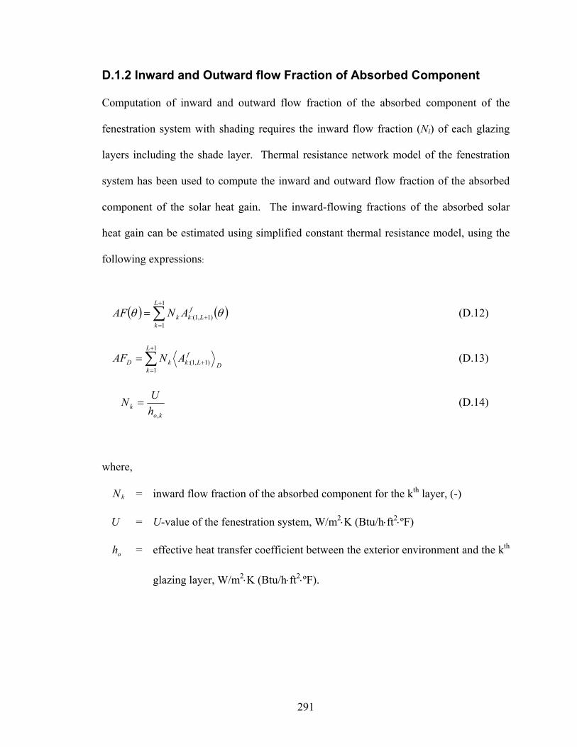
291
D.1.2 Inward and Outward flow Fraction of Absorbed Component
Computation of inward and outward flow fraction of the absorbed component of the
fenestration system with shading requires the inward flow fraction (Ni) of each glazing
layers including the shade layer. Thermal resistance network model of the fenestration
system has been used to compute the inward and outward flow fraction of the absorbed
component of the solar heat gain. The inward-flowing fractions of the absorbed solar
heat gain can be estimated using simplified constant thermal resistance model, using the
following expressions:
( ) ( )θθ ∑+
=+=
1
1)1,1(:
L
k
fLkk ANAF (D.12)
∑+
=+=
1
1)1,1(:
L
kD
fLkkD ANAF (D.13)
kok h
UN,
= (D.14)
where,
kN = inward flow fraction of the absorbed component for the kth layer, (-)
U = U-value of the fenestration system, W/m2⋅K (Btu/h⋅ft2⋅ºF)
oh = effective heat transfer coefficient between the exterior environment and the kth
glazing layer, W/m2⋅K (Btu/h⋅ft2⋅ºF).
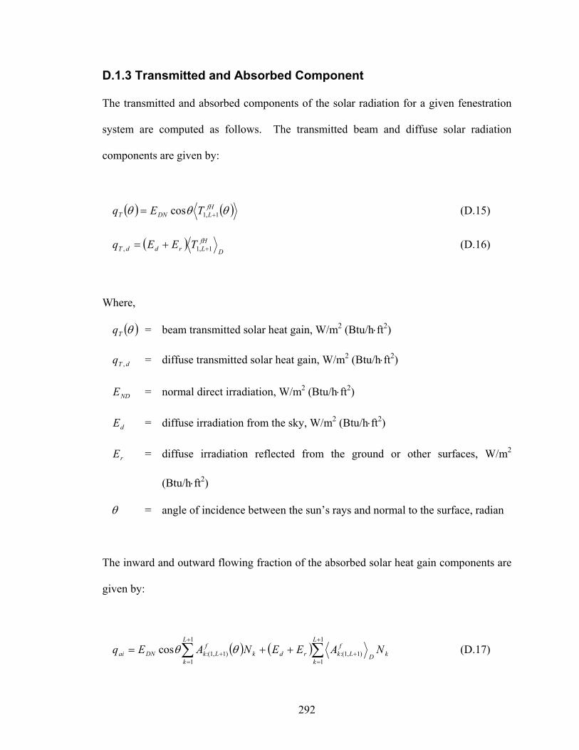
292
D.1.3 Transmitted and Absorbed Component
The transmitted and absorbed components of the solar radiation for a given fenestration
system are computed as follows. The transmitted beam and diffuse solar radiation
components are given by:
( ) ( )θθθ fHLDNT TEq 1,1cos += (D.15)
( )D
fHLrddT TEEq 1,1, ++= (D.16)
Where,
( )θTq = beam transmitted solar heat gain, W/m2 (Btu/h⋅ft2)
dTq , = diffuse transmitted solar heat gain, W/m2 (Btu/h⋅ft2)
NDE = normal direct irradiation, W/m2 (Btu/h⋅ft2)
dE = diffuse irradiation from the sky, W/m2 (Btu/h⋅ft2)
rE = diffuse irradiation reflected from the ground or other surfaces, W/m2
(Btu/h⋅ft2)
θ = angle of incidence between the sun’s rays and normal to the surface, radian
The inward and outward flowing fraction of the absorbed solar heat gain components are
given by:
( ) ( )∑∑+
=+
+
=+ ++=
1
1)1,1(:
1
1)1,1(:cos
L
kkD
fLkrd
L
kk
fLkDNai NAEENAEq θθ (D.17)
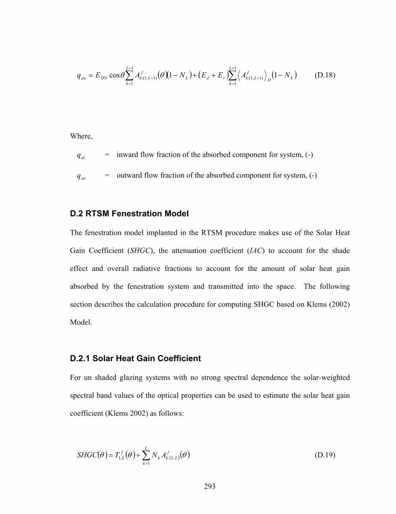
293
( )( ) ( ) ( )∑∑+
=+
+
=+ −++−=
1
1)1,1(:
1
1)1,1(: 11cos
L
kkD
fLkrd
L
kk
fLkDNao NAEENAEq θθ (D.18)
Where,
aiq = inward flow fraction of the absorbed component for system, (-)
aoq = outward flow fraction of the absorbed component for system, (-)
D.2 RTSM Fenestration Model
The fenestration model implanted in the RTSM procedure makes use of the Solar Heat
Gain Coefficient (SHGC), the attenuation coefficient (IAC) to account for the shade
effect and overall radiative fractions to account for the amount of solar heat gain
absorbed by the fenestration system and transmitted into the space. The following
section describes the calculation procedure for computing SHGC based on Klems (2002)
Model.
D.2.1 Solar Heat Gain Coefficient
For un shaded glazing systems with no strong spectral dependence the solar-weighted
spectral band values of the optical properties can be used to estimate the solar heat gain
coefficient (Klems 2002) as follows:
( ) ( ) ( ) ( )∑=
+=L
k
fLkk
fL ANTSHGC
1,1:,1 θθθ (D.19)
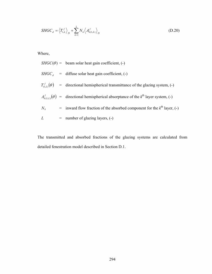
294
∑=
+=L
kD
fLkkD
fLd ANTSHGC
1),1(,1 (D.20)
Where,
)(θSHGC = beam solar heat gain coefficient, (-)
dSHGC = diffuse solar heat gain coefficient, (-)
( )θfLT ),1( = directional hemispherical transmittance of the glazing system, (-)
( )θfLkA ),1(: = directional hemispherical absorptance of the kth layer system, (-)
kN = inward flow fraction of the absorbed component for the kth layer, (-)
L = number of glazing layers, (-)
The transmitted and absorbed fractions of the glazing systems are calculated from
detailed fenestration model described in Section D.1.

VITA
Bereket Asgedom Nigusse
Candidate for the Degree of
Doctor of Philosophy Thesis: IMPROVEMENTS TO THE RADIANT TIME SERIES METHOD COOLING
LOAD CALCULATION PROCEDURE Major Field: Mechanical Engineering Biographical:
Personal Data: Date of Birth: Jan 30, 1966 Place of Birth: Asmara, Eritrea
Education:
Received Bachelor of Science degree in Chemical Engineering from Addis Ababa University, Addis Ababa, Ethiopia, in July 1989.
Received Master of Engineering Science in Mechanical Engineering from the University of New South Wales, Sydney, Australia, in May 1998.
Completed the requirements for the Doctor of Philosophy in Mechanical Engineering at Oklahoma State University, Stillwater, Oklahoma in December 2007.
Experience:
Aug 2005 - Present Graduate Research Associate Oklahoma State University Aug 2003 – July 2005 Fulbright Fellow Oklahoma State University
Professional Memberships: Phi Kappa Phi Honor Society, American Society of
Heating, Refrigerating and Air-conditioning Engineers (ASHRE), and International Building Performance Simulation Association (IBPSA).
ADVISER’S APPROVAL: Dr Jeffrey D. Spitler
Name: Bereket A. Nigusse Date of Degree: December, 2007 Institution: Oklahoma State University Location: Stillwater, Oklahoma Title of Study: IMPROVEMENTS TO THE RADIANT TIME SERIES METHOD
COOLING LOAD CALCULATION PROCEDURE Pages in Study: 294 Candidate for the Degree of Doctor of Philosophy
Major Field: Mechanical Engineering Scope and Method of Study: The objective of the study was improvement of the Radiant Time Series Method (RTSM) cooling load calculation procedure. A series of investigations were carried out, including: improvements to peak cooling load prediction performance, development of a simplified procedure for Radiant Time Factor (RTF) generation, adaptation of the fenestration sub-model to be compatible with currently available manufacturer’s data, establishing appropriate radiative fractions for all heat gain types. The simplified RTF generation procedure facilitates implementation in a range of computing environments. Furthermore, an approximate one-dimensional dynamic model for thermal bridges has been investigated and validated against both experimental results and detailed computational results. Findings and Conclusions: The Radiant Time Series Method was modified by introducing a dimensionless loss conductance that is readily calculable from the zone geometry and surface characteristic. Along with the revised fenestration sub-model, newly-recommended radiative fractions, and simplified RTF generation procedure, the RTSM performance was validated against the reference method, the heat balance method (HBM) with a large parametric study. The parametric study compared peak cooling loads determined with the improved RTSM procedure to those determined with the HBM for a wide range of building design parameters, for which all combinations formed 2,867,200 different zones. Use of the dimensionless loss conductance caused the maximum overprediction to go from 37% to 18%. Several additional simplifications were made to facilitate implementation in a range of computing environments. These simplifications included development of a one-dimensional finite volume numerical procedure for generating periodic response factors. This reduced the number of lines of source-code required with the previous state-space method from 2000 to 500 in Fortran 90. In a computing environment with embedded matrix algebra, such as SCILAB, the number of lines of source-code can be further reduced to 150. The new formulation of the RTF generation procedure allows very compact implementation (150 lines of source code, compared to the original procedure, implemented in approximately 4000 lines of Fortran 90 source code) in computing. The approximate one-dimensional dynamic model of thermal bridges has been validated against published experimental results and also against numerical results generated with a 2D finite volume program. The approximate model can predict peak heat gains within ±2.6% of the experimental measurements, provided accurate steady state thermal resistances are used.