Brigham Young University Brigham Young University

BYU ScholarsArchive BYU ScholarsArchive

Theses and Dissertations

2019-08-01

Improving and Modeling Bacteria Recovery in Hollow Disk System Improving and Modeling Bacteria Recovery in Hollow Disk System

Clifton Anderson Brigham Young University

Follow this and additional works at: https://scholarsarchive.byu.edu/etd

BYU ScholarsArchive Citation BYU ScholarsArchive Citation Anderson, Clifton, "Improving and Modeling Bacteria Recovery in Hollow Disk System" (2019). Theses and Dissertations. 8117. https://scholarsarchive.byu.edu/etd/8117

This Thesis is brought to you for free and open access by BYU ScholarsArchive. It has been accepted for inclusion in Theses and Dissertations by an authorized administrator of BYU ScholarsArchive. For more information, please contact scholarsarchive@byu.edu, ellen_amatangelo@byu.edu.

Improving and Modeling Bacteria Recovery in Hollow Disk System

Clifton Anderson

A thesis submitted to the faculty of

Brigham Young University

in partial fulfillment of the requirements for the degree of

Master of Science

William G. Pitt, Chair

David O. Lignell

Douglas R. Tree

Department of Chemical Engineering

Brigham Young University

Copyright © 2019 Clifton Anderson

All Rights Reserved

ABSTRACT

Improving and Modeling Bacteria Recovery in Hollow Disk System

Clifton Anderson

Department of Chemical Engineering, BYU

Master of Science

Identifying antibiotic resistance in blood infections requires separating bacteria from

whole blood. A hollow spinning disk rapidly removes suspended red blood cells by leveraging

hydrodynamic differences between bacteria and whole blood components in a centrifugal field.

Once the red cells are removed, the supernatant plasma which contains bacteria is collected for

downstream antibiotic testing.

This work improves upon previous work by modifying the disk design to maximize

fractional plasma recovery and minimize fractional red cell recovery. V-shaped channels induce

plasma flow and increase fractional plasma recovery. Additionally, diluting a blood sample

spiked with bacteria prior to spinning it increased the fractional bacteria recovery. A numerical

model for red cell sedimentation shows that red cells are removed from solution more rapidly as

the blood is diluted. Diluting blood is beneficial but may create too much biological waste. The

benefits of diluting are formulated as an optimization problem subject to the end user’s needs.

Keywords: sepsis, bacteremia, antibiotics, blood, sedimentation, modeling conservation laws

ACKNOWLEDGEMENTS

Thanks to National Institutes of Health (grant R01AI116989) for funding this research.

Many thanks also Dr. Bill Pitt for all his help with this project. I appreciated how available he

was for questions and how many ideas he helped form. Thanks also to Ryan Wood and Dr. John

Lawson for their helpful conversations. Evelyn Welling was an interested and helpful hand in my

bacteria experiments and in getting blood donations figured out. Thanks also to Jake Stepan,

Rebecca Prymak, and Caroline Hickey, who all plate bacteria much better than I. And last the

best of all the game, a huge thank you to my wife, Chelsea, for all her support and

encouragement.

iv

TABLE OF CONTENTS

LIST OF TABLES ......................................................................................................................... vi

LIST OF FIGURES ...................................................................................................................... vii

1 Introduction ............................................................................................................................. 1

2 Literature review ...................................................................................................................... 3

2.1 Stokes’ law ....................................................................................................................... 3

2.2 Hindered settling corrections ........................................................................................... 4

2.3 Converting from slip velocity to absolute velocity .......................................................... 7

2.4 Equation formulation........................................................................................................ 8

2.4.1 Conservation law formulation................................................................................... 8

2.4.2 Characteristic structure and the sedimentation flux curve ........................................ 9

2.5 Integration ...................................................................................................................... 12

2.5.1 Method of characteristics ........................................................................................ 12

2.5.2 Numerical integration ............................................................................................. 14

3 Methods and materials ........................................................................................................... 17

3.1 Definitions and disk naming scheme ............................................................................. 17

3.2 Rapid prototyping ........................................................................................................... 19

3.3 Contact angle measurements .......................................................................................... 20

3.4 Wafer experiments ......................................................................................................... 21

3.4.1 Polymer coatings ..................................................................................................... 23

3.5 Spinning experiments ..................................................................................................... 23

3.5.1 Disk preparation and spinning ................................................................................ 23

3.5.2 Bacteria preparation and counting .......................................................................... 25

3.5.3 Definition of plasma, red cell and bacteria recoveries ............................................ 25

3.6 Statistics ......................................................................................................................... 28

4 Experimental results and discussion of disk designs ............................................................. 29

4.1 Contact angle .................................................................................................................. 29

4.2 Liquids on tilted wafers .................................................................................................. 33

4.3 Disk weir design ............................................................................................................. 35

4.3.1 Glossy ..................................................................................................................... 35

4.3.2 Ruffles ..................................................................................................................... 35

v

4.3.3 Wells ....................................................................................................................... 37

4.4 Flowdown volume .......................................................................................................... 38

4.5 Plasma recovery ............................................................................................................. 38

4.5.1 Weir width .............................................................................................................. 39

4.5.2 Effect of weir slope designs .................................................................................... 41

4.5.3 Effect of collection time.......................................................................................... 42

4.6 Red cell recovery ............................................................................................................ 43

4.6.1 Trough volume ........................................................................................................ 44

4.6.2 Weir width .............................................................................................................. 45

4.6.3 Baffles ..................................................................................................................... 46

4.6.4 Ruffles ..................................................................................................................... 47

4.7 Summary ........................................................................................................................ 48

5 Modeled and experimental effects of blood dilution ............................................................. 50

5.1 Sedimentation time ......................................................................................................... 50

5.2 Bacteria recovery............................................................................................................ 58

5.3 Dilution optimization ..................................................................................................... 62

5.4 Summary ........................................................................................................................ 64

6 Conclusions and recommendations ....................................................................................... 65

6.1 Conclusions .................................................................................................................... 65

6.1.1 Aim 1: disk designs ................................................................................................. 65

6.1.2 Aim 2: blood dilution and bacteria recovery .......................................................... 66

6.1.3 Aim 3: numerical model of sedimentation .............................................................. 67

6.2 Recommendations for future research............................................................................ 68

References ..................................................................................................................................... 70

Appendix A ................................................................................................................................... 75

A.1 Tables ............................................................................................................................. 75

A.2 Figures ............................................................................................................................ 78

A.3 Hematocrit calibration .................................................................................................... 79

A.4 Experimental sedimentation profiles .............................................................................. 80

A.5 Effect of long hold time on plasma recovery ................................................................. 80

A.6 Numerical model code ................................................................................................... 81

vi

LIST OF TABLES

Table 1 Contact angles for plasma and water on wafers. ............................................................. 30 Table 2 Physical properties of blood and bacteria. ....................................................................... 75 Table 3 Recovery values for 32 factorial experiments. ................................................................. 75 Table 4 Summary of flowdown mass, plasma recovery, and red cell recovery for all disks. ...... 76 Table 5 Selected dimensions for disks. ......................................................................................... 77

vii

LIST OF FIGURES

Figure 1 Dimensionless red cell flux curve and characteristic speed versus hematocrit .............. 11 Figure 2 Example of sedimentation profile for red blood cells and white blood cells. ................ 13 Figure 3 Schematic of a disk, including design features. ............................................................. 18 Figure 4 Example of a test wafer. ................................................................................................. 22 Figure 5 Contact angle of plasma-saline dilutions on plasma-coated 3D printed wafers. ............ 32 Figure 6 Summary of PEO coating effect on inclination angles for consecutive cycles .............. 33 Figure 7 Breakthrough points associated with short and long ruffles. ......................................... 36 Figure 8 Photographs showing breakthrough on different disks. ................................................. 38 Figure 9 Volumetric flowdown for all disks. ................................................................................ 39 Figure 10 Plasma Recovery for all disks. ..................................................................................... 40 Figure 11 Red cell recovery versus whole blood hematocrit for feature categories. .................... 43 Figure 12 Red cell recovery versus hematocrit for trough volumes of 3, 4 and 5 mL.... 45 Figure 13 Red cell recovery for 3 pairs of baffled and unmodified (i.e. base) disks........... 46 Figure 14 Red cell recovery vs plasma recovery grouped by disk type. ...................................... 47 Figure 15 Paired plasma and red cell recovery for disks channel depth 0.05 and 0.035 inch. ..... 48 Figure 16 Red cell sedimentation profiles for a range of initial hematocrits (0.05,0.21,0.47). .... 53 Figure 17 Non-dimensional sedimentation time as a function of hematocrit. .............................. 55 Figure 18 Comparison of experimental and numerical model of red cell sedimentation. ............ 57 Figure 19 Concentration recovery as a function of hematocrit..................................................... 60 Figure 20 Bacteria recovery as a function of hematocrit .............................................................. 60 Figure 21 Example curves for the bacterial recovery optimization. ............................................. 63 Figure 22 Red cell recovery versus whole blood hematocrit for individual disks........................ 78 Figure 23 Ratio of Stokes velocities to induce backflow in a 2-component suspension. ............. 78 Figure 24 Hematocrit calibration for lab centrifuge and clinical centrifuge. ............................... 79 Figure 25 Experimental sedimentation profiles in a flat, cylindrical disk .................................... 80 Figure 26 Fluid loss with spin time............................................................................................... 81

1

1 INTRODUCTION

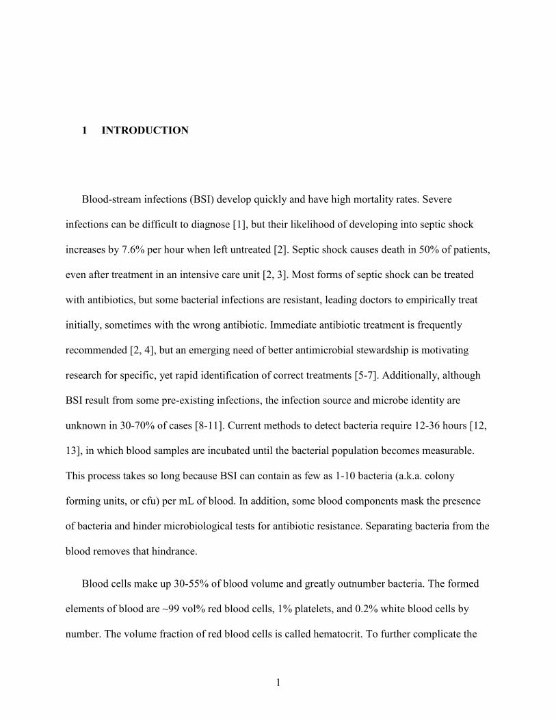
Blood-stream infections (BSI) develop quickly and have high mortality rates. Severe

infections can be difficult to diagnose [1], but their likelihood of developing into septic shock

increases by 7.6% per hour when left untreated [2]. Septic shock causes death in 50% of patients,

even after treatment in an intensive care unit [2, 3]. Most forms of septic shock can be treated

with antibiotics, but some bacterial infections are resistant, leading doctors to empirically treat

initially, sometimes with the wrong antibiotic. Immediate antibiotic treatment is frequently

recommended [2, 4], but an emerging need of better antimicrobial stewardship is motivating

research for specific, yet rapid identification of correct treatments [5-7]. Additionally, although

BSI result from some pre-existing infections, the infection source and microbe identity are

unknown in 30-70% of cases [8-11]. Current methods to detect bacteria require 12-36 hours [12,

13], in which blood samples are incubated until the bacterial population becomes measurable.

This process takes so long because BSI can contain as few as 1-10 bacteria (a.k.a. colony

forming units, or cfu) per mL of blood. In addition, some blood components mask the presence

of bacteria and hinder microbiological tests for antibiotic resistance. Separating bacteria from the

blood removes that hindrance.

Blood cells make up 30-55% of blood volume and greatly outnumber bacteria. The formed

elements of blood are ~99 vol% red blood cells, 1% platelets, and 0.2% white blood cells by

number. The volume fraction of red blood cells is called hematocrit. To further complicate the

2

problem of separation, bacterial and red blood cell specific gravities tend to overlap. Fortunately,

their hydrodynamic properties do not. Red blood cells (RBCs) sediment about 30 times faster

than bacteria because they are larger than most bacteria (5-8 µm diameter vs 1-4 µm for RBCs

and bacteria, respectively). Most methods reported in the literature leverage hydrodynamic

differences to separate blood cells and bacteria. For example, Dr. Pitt’s group has developed a

centrifugal disk that uses 7 mL of blood and quickly sediments the RBCs out of suspension,

leaving bacteria in the plasma [14]. This process takes about 5 minutes, and the bacteria-laden

plasma has fewer red cells than the original whole blood sample.

Previous work on this separation process focused on disk modifications to recover more

plasma and fewer red cells, as well as exploring the effect of spin time and disk speed (angular

velocity) on bacterial recovery. It succeeded in recovering an average 70% of the plasma, 5-20%

of the red cells, and 60% of the bacteria during a total spin time of ~3 minutes.

This work pursues similar aims. Its primary objectives are to maximize recovered bacteria

and minimize red cells in the recovered plasma. It focuses on (1) iterative improvements for

recovering more plasma and fewer red cells and briefly explores the effect on plasma recovery of

polymer coatings on the disk. Another main objective is (2) to explore how diluting the blood

prior to spinning affects optimal spin time and bacteria recovery. Finally, it aims to (3) develop a

numerical model of simultaneous sedimentation of particles in blood to explore and optimize

process design.

3

2 LITERATURE REVIEW

This chapter begins by describing how body forces and solids concentration affect the speed

of blood cells and bacteria in a suspension. It then sets up the mathematical framework for

describing sedimentation and finishes by giving a brief overview of integration methods used in

this thesis. It does not focus on contemporary technology for identifying antibiotic resistance.

For that, the reader is referred to a recent article by Pitt et al. [15].

In this thesis, the term “suspension” is defined as a mixture of fluid and particles in which the

particles are not in continuous contact with each other or with the wall. In this thesis, it most

commonly refers to a layer of cells (potentially of different type) surrounded by blood plasma. In

contrast, the term “sediment” refers to the region in the spatial domain comprised of cells that are

either touching the wall or that are in continuous contact with cells that are touching the wall.

“Sedimentation” refers to the movement of cells in the direction of body force applied by a

gravitational or a centrifugal field. Finally, the “clear fluid” region has no suspended cells.

2.1 Stokes’ law

The steady state velocity of particles in a centrifugal field can be predicted at Re<<1 using

Stokes’ law (Equation 2-1). This law gives the drag force on a rigid sphere in creeping flow at

infinite dilution (i.e. no interparticle interactions) as a function of fluid viscosity (𝜇), particle

diameter (𝐷), and particle velocity (𝑢) relative to the suspending fluid:

4

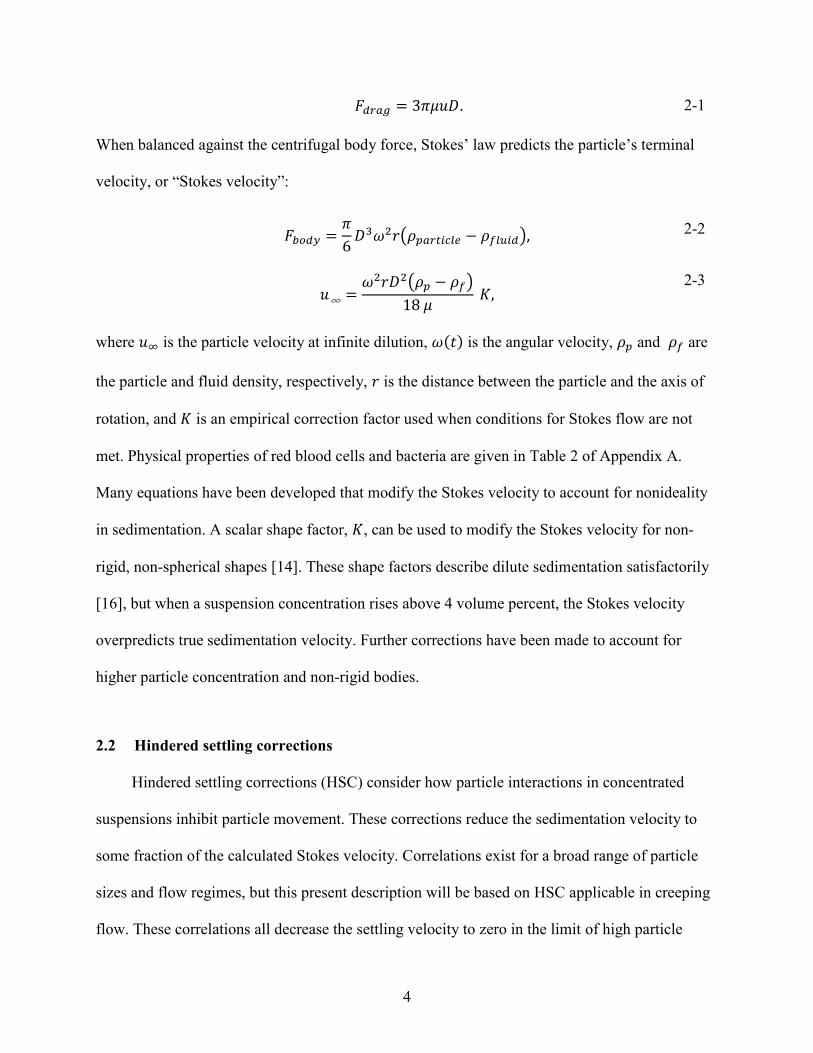
𝐹𝑑𝑟𝑎𝑔 = 3𝜋𝜇𝑢𝐷. 2-1

When balanced against the centrifugal body force, Stokes’ law predicts the particle’s terminal

velocity, or “Stokes velocity”:

𝐹𝑏𝑜𝑑𝑦 =𝜋

6𝐷3𝜔2𝑟(𝜌𝑝𝑎𝑟𝑡𝑖𝑐𝑙𝑒 − 𝜌𝑓𝑙𝑢𝑖𝑑), 2-2

𝑢∞ =

𝜔2𝑟𝐷2(𝜌𝑝 − 𝜌𝑓)

18 𝜇 𝐾,

2-3

where 𝑢∞ is the particle velocity at infinite dilution, 𝜔(𝑡) is the angular velocity, 𝜌𝑝 and 𝜌𝑓 are

the particle and fluid density, respectively, 𝑟 is the distance between the particle and the axis of

rotation, and 𝐾 is an empirical correction factor used when conditions for Stokes flow are not

met. Physical properties of red blood cells and bacteria are given in Table 2 of Appendix A.

Many equations have been developed that modify the Stokes velocity to account for nonideality

in sedimentation. A scalar shape factor, 𝐾, can be used to modify the Stokes velocity for non-

rigid, non-spherical shapes [14]. These shape factors describe dilute sedimentation satisfactorily

[16], but when a suspension concentration rises above 4 volume percent, the Stokes velocity

overpredicts true sedimentation velocity. Further corrections have been made to account for

higher particle concentration and non-rigid bodies.

2.2 Hindered settling corrections

Hindered settling corrections (HSC) consider how particle interactions in concentrated

suspensions inhibit particle movement. These corrections reduce the sedimentation velocity to

some fraction of the calculated Stokes velocity. Correlations exist for a broad range of particle

sizes and flow regimes, but this present description will be based on HSC applicable in creeping

flow. These correlations all decrease the settling velocity to zero in the limit of high particle

5

density: 𝑙𝑖𝑚𝜙→𝜙𝑚𝑎𝑥

𝑢

𝑢∞= 0, where 𝜙 is the volumetric particle concentration. Many authors have

investigated the hydrodynamics of dilute and concentrated suspensions of rigid spheres [17-24].

When modeling meso to macro scale sedimentation specifically, the most common HSC range

from empirical to semi-empirical for practical conditions [25-33].

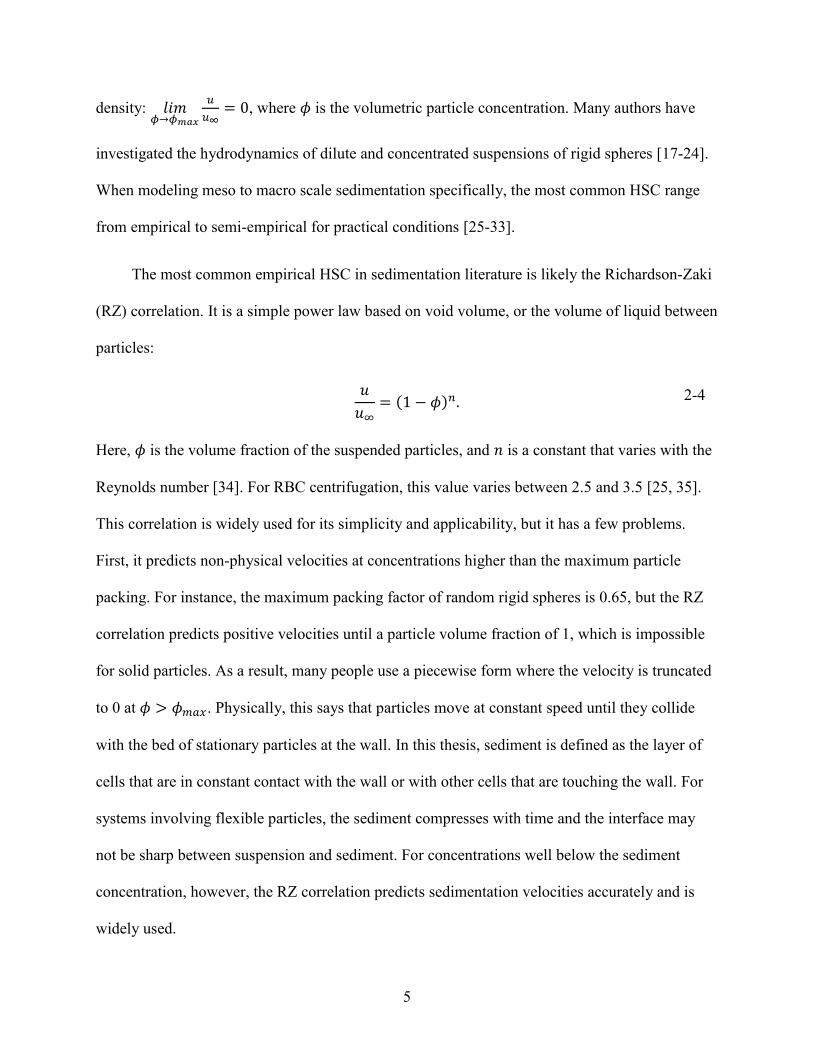
The most common empirical HSC in sedimentation literature is likely the Richardson-Zaki

(RZ) correlation. It is a simple power law based on void volume, or the volume of liquid between

particles:

𝑢

𝑢∞= (1 − 𝜙)𝑛. 2-4

Here, 𝜙 is the volume fraction of the suspended particles, and 𝑛 is a constant that varies with the

Reynolds number [34]. For RBC centrifugation, this value varies between 2.5 and 3.5 [25, 35].

This correlation is widely used for its simplicity and applicability, but it has a few problems.

First, it predicts non-physical velocities at concentrations higher than the maximum particle

packing. For instance, the maximum packing factor of random rigid spheres is 0.65, but the RZ

correlation predicts positive velocities until a particle volume fraction of 1, which is impossible

for solid particles. As a result, many people use a piecewise form where the velocity is truncated

to 0 at 𝜙 > 𝜙𝑚𝑎𝑥. Physically, this says that particles move at constant speed until they collide

with the bed of stationary particles at the wall. In this thesis, sediment is defined as the layer of

cells that are in constant contact with the wall or with other cells that are touching the wall. For

systems involving flexible particles, the sediment compresses with time and the interface may

not be sharp between suspension and sediment. For concentrations well below the sediment

concentration, however, the RZ correlation predicts sedimentation velocities accurately and is

widely used.

6

Corrections that are valid over the entire domain of concentrations have also been

developed. These tend to be more theoretical, though still quite empirical. For example, the

Michaels correlation is an amendment to the RZ correlation that restricts the domain to 𝜙 ∈

[0, 𝜙𝑚𝑎𝑥] [31]. It is as follows:

𝑢

𝑢∞= (1 −

𝜙

𝜙𝑚𝑎𝑥)

𝑛𝑑𝑒𝑓𝜙𝑚𝑎𝑥

, 2-5

where 𝑛𝑑𝑒𝑓 is a parameter describing particle deformability. This equation predicts a zero

velocity at maximum packing. Whereas the (clipped) RZ correlation physically implies that

particles collide with a sediment and stop instantaneously to form a clear suspension-sediment

interface, the Michaels correlation slowly decreases the particle velocity to zero and does not

distinguish a cutoff ϕ between suspension and sediment. This is valuable because red blood cells

are extremely flexible: reported maximum packing factors of RBCs range from 0.8 [36] to 0.97

[37] depending on the strength and duration of the centrifugal field. One group emphasized the

slow compaction of the red cell sediment by combining the RZ and Michaels correlations in the

following way [36]:

𝑢

𝑢∞= (1 − 𝜙)2 (1 −

𝜙

𝜙𝑚𝑎𝑥)

𝑛𝑑𝑒𝑓𝜙𝑚𝑎𝑥

. 2-6

Here, the Michaels correlation is used to simulate the viscosity of the red cell sediment. Lerche et

al. showed that this form accurately modeled RBC sedimentation and compaction for a broad

range of hematocrits using 𝑛𝑑𝑒𝑓 = 2.71. This model represents RBC sedimentation profiles well,

especially at high hematocrit.

HSC also exist for particle mixtures. For example, the Masliyah-Lockett-Bassoon (MLB)

[38] correlation is a generalized form of the RZ correlation. Another HSC describes the

7

“apparent porosity,” or average interparticle spacing as a concentration-weighted sum of particle

diameters [35, 39].

2.3 Converting from slip velocity to absolute velocity

Stokes’ law and many HSC describe the slip velocity, or velocity of the particle relative to

the fluid. However, a stationary reference frame models the particle velocity with respect to the

disk instead of to the fluid. A volume balance on aggregate particle movement converts from slip

velocity 𝑢 to absolute velocity 𝑣 [29]:

𝑣𝑖 =  𝑢𝑖 − ∑ 𝑢𝑗𝜙𝑗

𝑁

𝑗=1

. 2-7

for the 𝑖𝑡ℎ species (including plasma if desired) summed over all 𝑁 species. The result does not

change when plasma is considered because the slip velocity of plasma relative to itself is zero.

The term in the summation is the volume average suspension velocity and represents backward

fluid flow. Equation 2-7 allows us to calculate the plasma velocity. For a single particle type, this

equation simplifies to:

𝑣 = 𝑢(1 − 𝜙). 2-8

Hence, the absolute velocity is always smaller than the slip velocity. When reading about

an unfamiliar HSC, it is important to note whether it modifies the slip or the absolute velocity.

Failure to do so can bias velocity estimates by a factor of (1 − 𝜙)±1.

8

2.4 Equation formulation

2.4.1 Conservation law formulation

The theory for sedimentation processes was pioneered by Kynch in 1954, who described

the convective flux of particles along an accelerating field as a function of local concentration. In

conservation form and Cartesian coordinates, the hyperbolic system of PDEs describing such

particle sedimentation can be written as follows:

∂Φ

∂t+ ∇ ⋅ 𝐹(𝚽) = 0,

2-9

where Φ is a vector of 𝐽 volume fractions for each possible cell type (e.g. red cells, white cells,

platelets, bacteria). The vector function F(Φ) is referred to in some literature as the “batch

Kynch flux function” [28] and is the volumetric particle flux. It is the product of species volume

fraction and absolute velocity (i.e. 𝐹𝑗(Φ) = Φj𝑣𝑗(Φ)). For multicomponent systems, the

dependence of F(Φ) on the entire vector of volume fractions Φ makes this a coupled system of

equations. This is a continuum approach that considers the cells as incompressible liquid phases

and does not explicitly model the plasma. Thus, a system with one particle type suspended in

fluid is called a 2-component system, but it is a scalar equation.

This model does not account for any particle diffusion [40], but some models have used a

diffusive term to describe sediment compression [28, 41, 42]. Equation 2-6 given by Lerche does

not consider the sediment specially. One benefit of casting the problem as the continuity

equation is the wide base of knowledge for integrating conservation laws. Integration schemes

can have very rigid constraints, however. Tory modeled multicomponent hindered settling using

a stochastic particle-based approach that provided some extra modeling flexibility [43].

9

2.4.2 Characteristic structure and the sedimentation flux curve

Applying the chain rule to the 1D scalar (2 component) form of Equation 2-9 converts it

into characteristic form:

𝜕𝜙

𝜕𝑡+

𝜕𝑓

𝜕𝜙

𝜕𝜙

𝜕𝑥= 0. 2-10

Here, f is the scalar form of the flux function F. Characteristic form represents the continuity

equation in a different perspective. Whereas the conservation form is reminiscent of material

balances and the familiar divergence theorem, the characteristic form represents the continuity

equation more like a wave. In characteristic form, the continuity equation becomes a wave of

height 𝜙(𝑥, 𝑡) that moves in the x-t plane at speed 𝜕𝑓/𝜕𝜙, or 𝑓′(𝜙). Values of 𝜙 remain

constant along curves referred to as characteristics that have slope 𝑑𝑥/𝑑𝑡 = 𝑓′(𝜙). If the flux

function has no spatial dependence, then characteristics are straight lines. Characteristics are the

path that the wave 𝜙(𝑥, 𝑡) takes in the x-t plane. It is important to note that the speeds of

characteristics are conceptually different than the physical speed of the red cells. Characteristics

are a mathematical construct that represent the direction and speed of information propagation.

They span the entire spatial and temporal domain until they either exit the domain or intersect

with another characteristic.

When characteristics spread away from each other, a rarefaction wave forms through

which 𝜙(𝑥, 𝑡) varies smoothly. On the other hand, when characteristics intersect, a discontinuity

in ϕ forms with states 𝜙𝐿 and 𝜙𝑅 associated with the characteristics to the left and right of the

discontinuity. This is known as a shock. The shock speed 𝑠 is obtained by the Rankine-Hugoniot

jump condition 𝑠 =𝑓(𝜙𝑅)−𝑓(𝜙𝐿)

𝜙𝑅−𝜙𝐿, which can be thought of as a material balance. With a given flux

curve, however, the Rankine-Hugoniot condition can predict shock speeds that are not physically

10

valid. To prevent this, shock speeds are subjected to a so-called “entropy condition”. One such

condition is the Oleinik entropy condition 𝑓(𝜙)−𝑓(𝜙𝐿)

𝜙−𝜙𝐿≤ 𝑠 ≤

𝑓(𝜙)−𝑓(𝜙𝑅)

𝜙−𝜙𝑅, where 𝜙 ∈ [𝜙𝐿 , 𝜙𝑅].

What this says is that the shock speed is bounded by the speed of the characteristics that collided.

For non-convex flux functions, it is sometimes impossible to connect two states by a

shock without generating unphysical solutions because the line connecting two states must not

cross the flux curve. In this case, the unphysical shock is mathematically restated as a

combination of shock and a rarefaction, which are both physically valid, connected by an

intermediate state ϕ𝑟𝑎𝑟𝑒. Finding the states across this new combined shock-rarefaction involves

constructing a convex hull (see Figure 1) (a.k.a. the “stretched string analogy” or “rubber band

method”) around the flux curve. The tangency point in the convex hull ϕ𝑟𝑎𝑟𝑒 is the state on the

rarefaction side of the shock in the new shock-rarefaction combination (see Section 16.1.2 of

[44]).

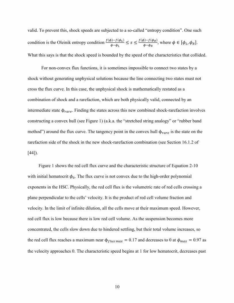
Figure 1 shows the red cell flux curve and the characteristic structure of Equation 2-10

with initial hematocrit 𝜙0. The flux curve is not convex due to the high-order polynomial

exponents in the HSC. Physically, the red cell flux is the volumetric rate of red cells crossing a

plane perpendicular to the cells’ velocity. It is the product of red cell volume fraction and

velocity. In the limit of infinite dilution, all the cells move at their maximum speed. However,

red cell flux is low because there is low red cell volume. As the suspension becomes more

concentrated, the cells slow down due to hindered settling, but their total volume increases, so

the red cell flux reaches a maximum near ϕ𝑓𝑙𝑢𝑥 𝑚𝑎𝑥 = 0.17 and decreases to 0 at 𝜙𝑚𝑎𝑥 = 0.97 as

the velocity approaches 0. The characteristic speed begins at 1 for low hematocrit, decreases past

11

0 at ϕ𝑓𝑙𝑢𝑥 𝑚𝑎𝑥 to a minimum at the flux inflection point ϕ𝑖𝑛𝑓𝑙𝑒𝑐 = 0.348 and slowly raises back

up to 0 as ϕ approaches ϕ𝑚𝑎𝑥.

Figure 1 Dimensionless red cell flux curve and characteristic speed versus hematocrit showing

shock and rarefaction curves. Blue solid line shows red cell flux normalized by red cell Stokes

velocity using Lerche’s hindered settling correction. Green dashed line shows the derivative of

the red cell flux showing the speed of characteristics versus wave height (i.e. hematocrit). Black

line with points shows the convex hull that connects each state by shocks (straight lines) and

rarefaction (curved portion).

An interesting result of the characteristic form is that shocks represent interfaces between

different regions of the suspension. Consider the initial profile 𝜙(𝑥, 𝑡) = 𝜙0 with boundary

conditions 𝜙(0, 𝑡) = 0 representing clear plasma and 𝜙(𝑥 = 𝐿, 𝑡) = 𝜙𝑚𝑎𝑥 representing

compacted cells at the disk wall. At 𝑥 = 0, there are no red cells; the characteristic speed is +1,

and the value 𝜙 = 0 enters the domain from the left for all t. In the middle of the domain, the

initial profile 𝜙(𝑥, 𝑡) = 𝜙0 advects along characteristics with the speed 𝑓′(𝜙0), but it is

overtaken by the faster-moving characteristics coming from the boundary at 𝑥 = 0. This forms a

12

shock with the states 𝜙𝐿 = 0 and 𝜙𝑅 = 𝜙0 which moves at the speed 𝑠 =𝑓(𝜙0)−𝑓(0)

𝜙0−0=

𝑓(𝜙0)

𝜙0=

𝑣(𝜙0). This shock is the suspension-clear fluid (SC) interface.

A more complex interaction between characteristics occurs on the right side of the domain

(𝑥 = 𝐿) where the right boundary 𝜙𝑚𝑎𝑥 is a stationary wave (𝜕𝑓/𝜕𝜙 = 0). The initial

discontinuity between 𝜙0 and 𝜙𝑚𝑎𝑥 cannot generate a shock without violating an entropy

condition, and a combined shock-rarefaction occurs, as previously described. Between the states

𝜙0 and 𝜙𝑟𝑎𝑟𝑒, a shock forms that represents the interface between suspended red blood cells and

the beginning of a red cell sediment. This is the suspension-sediment (SS) interface, and it moves

with speed 𝑠 =𝑓(𝜙𝑟𝑎𝑟𝑒)−𝑓(𝜙0)

𝜙𝑟𝑎𝑟𝑒−𝜙0. On the right side of the interface is the sediment, in which 𝜙

varies smoothly from 𝜙𝑟𝑎𝑟𝑒 to 𝜙𝑚𝑎𝑥. The value of characteristics is that the SS and SC interfaces

can be tracked simply by finding shock speeds.

2.5 Integration

2.5.1 Method of characteristics

The method of characteristics is an analytical method for solving hyperbolic equations by

tracing the characteristics of a hyperbolic equation to find a final solution. For simple scalar

conservation laws, the solution may be a simple piecewise function. In fact, some authors have

solved sedimentation problems using this method by explicitly tracking interface positions [45,

46]. Using the method of characteristics for systems of nonlinear equations, however, involves

decoupling the system by diagonalizing the Jacobian matrix ∂𝐹/ ∂Φ and expressing Φ(x, t) as a

linear combination of the Jacobian’s eigenvectors.

13

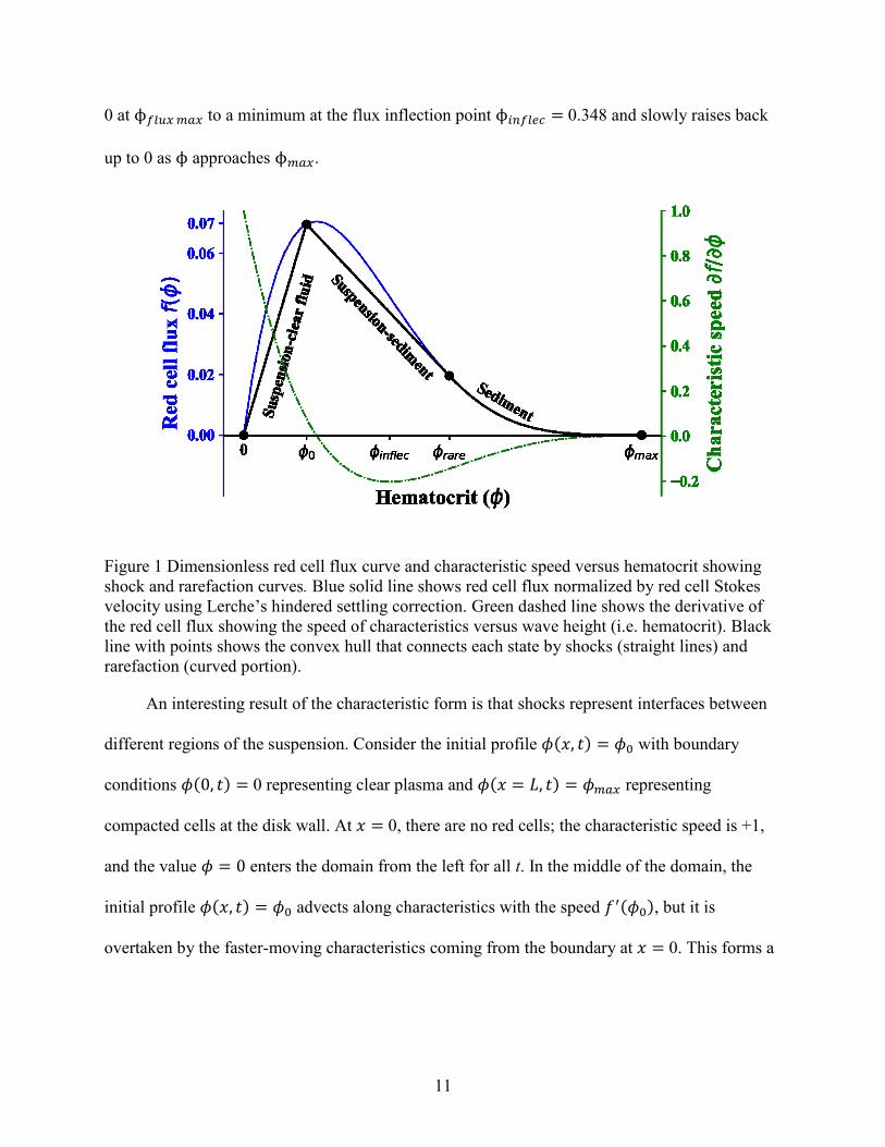
Notably, Sartory solved the sedimentation problem for a 3-component system of

granulocytes (small white blood cells) and red blood cells [47]. His method was mostly

analytical, and Figure 2 shows an example of his solution. The left axis shows dimensionless

height with gravity pointing downward to the tube bottom. The original suspension is a mix of

red blood cells at Φ0𝑅 = 0.25 and white blood cells at Φ0

𝑊 = 0.001. As time progresses, a

sediment layer consisting of red cells and granulocytes extends up from the tube bottom.

Granulocyte concentration in this layer decreased because his equations accounted for them

being less dense than red cells [30]. This differs from our system because bacteria and red cell

densities overlap. His solution shows two distinct suspended layers: (1) the original mixture and

(2) a pure granulocyte suspension whose concentration exceeds the starting concentration. Each

layer travels at a constant rate until it reaches the sediment layer. Sartory measured the number

of recoverable granulocytes as the thickness of the pure granulocyte layer multiplied by its

concentration.

Figure 2 Example of sedimentation profile for red blood cells (𝐶0𝑅 = 0.25) and white blood cells

(𝐶0𝑊=0.0011). Interfaces: – ; rarefaction in the sediment: – –. Reproduced with permission from

[47].

14

Sartory’s result is very interesting for our process for several reasons. Although other

authors have shown distinct suspended layers [48-50], Sartory’s solution highlights that

concentration of the slower particle in its pure suspension was enriched relative to its starting

concentration. That is interesting because it means that bacteria may be recoverable at a higher

concentration than their initial concentration. We are aware of no other work that predicts a

relationship between this enrichment of the second component in the supernatant fluid as a

function of the the volume fraction of the first component.

2.5.2 Numerical integration

Numerical integration schemes for sedimentation need to account for discontinuities caused

by interfaces and for non-convexity. Solutions to a kth order PDE that are k-times differentiable

and satisfy the PDE are known as “strong” solutions. Traditional finite difference schemes

derived from Taylor series assume strong solutions and can fail for problems with inherent

discontinuities. Instead, dealing with an integrated form of the PDE removes the need for

continuous derivatives. Solutions to the integrated PDE are called “weak” solutions because they

only satisfy one form of the PDE. Weak solutions arise frequently in physical systems. Not all

weak solutions are unique, however, which necessitates extra care via the entropy condition

briefly discussed in Section 2.4.2.

Integrating the conservation law Equation 2-9 serves as the basis for a finite volume

scheme. The steps involve integrating over the control volume 𝑉𝑖 (Equation 2-11), using the

divergence theorem to convert the second term to a surface integral (Equation 2-12), and

converting Φ to the volume-average Φ (Equation 2-13):

15

∭ (

∂Φ

∂𝑡+ ∇ ⋅ 𝐹(Φ)) 𝑑𝑉

𝑉𝑖

= 0, 2-11

∭

∂Φ

∂t𝑑𝑉

𝑉𝑖

+ ∯ (𝐹(Φ) ⋅ 𝑛)𝑑𝑆𝑆𝑖

= 0, 2-12

∂Φ

∂𝑡+

1

𝑉𝑖∯ (𝐹(Φ) ⋅ 𝑛)𝑑𝑆

𝑆𝑖

= 0. 2-13

For 1D, 𝑛 is a piecewise constant vector that points outward normal, and 𝑉𝑖 = 𝛥𝑥𝑖, such that

Equation 2-13 becomes

∂Φ

∂𝑡+

1

𝑥𝑖(𝐹(Φ𝑖+1/2) − 𝐹(Φ𝑖−1/2)) = 0. 2-14

Converting the time derivative to a forward difference and solving for Φ𝑘+1 yields the

discretized equation

Φ𝑘+1 = Φ𝑘 +

Δ𝑡

Δ𝑥𝑖(𝐹(Φ𝑖+1/2) − 𝐹(Φ𝑖−1/2)), 2-15

which provides an explicit time-marching scheme this is the basis for many finite volume

schemes. For the case of a single cell-type, Φ and F(Φ) become 𝜙 and 𝑓(𝜙), respectively.

Appropriately approximating interface flux values F(Φ) represents the major (and subtle)

differences between finite volume integration schemes. This section does not attempt to review

these methods, but rather to describe the method used in this work: Godunov’s method [51]. For

simplicity, this discussion will restrict itself to the scalar, or 2-component case1. It treats each

discontinuity in ϕ(x, t) as a Riemann problem centered on the interface between grid cells. A

Riemann problem is a conservation law with the discontinuous initial condition

1 The book “Finite Volume Methods for Hyperbolic Problems” by Randall LeVeque is a fantastic resource for

understanding the Riemann problem for many components and dimensions.

16

ϕ0 = {

𝜙𝐿 𝑥 < 𝑥0

𝜙𝑅 𝑥 > 𝑥0, 2-16

where the wave speed on either side of the discontinuity is given initially by 𝑓′(𝜙0). The

solution to the Riemann problem is the value 𝜙(𝑥𝑜) just after the wave begins to move. The

method is well suited for finite volume integration methods because each interface of the profile

ϕ(𝑥, 𝑡) can be thought of as a Riemann problem, the solution to which provides the interface

values for the fluxes in Equation 2-15. Godunov’s flux function provides the flux at a cell

interface by treating the interface as a Riemann problem:

𝑓 = {𝑚𝑖𝑛

𝜙𝐿≤𝜃≤𝜙𝑅

𝑓 (𝜃), 𝜙𝐿 < 𝜙𝑅

𝑚𝑎𝑥𝜙𝑅≤𝜃≤𝜙𝐿

𝑓 (𝜃), 𝜙𝐿 > 𝜙𝑅 . 2-17

This function is derived from a case-by-case analysis of Riemann problems. It generalizes the

upwind scheme and gives the entropy-satisfying (a.k.a. physical) solution even for non-convex

flux functions. Godunov’s method uses Equation 2-15 with the Godunov flux function (Equation

2-17) and is spatially 1st order accurate when using the piecewise-constant approximation

ϕ(𝑥, 𝑡). Higher order approximations to ϕ(𝑥, 𝑡) achieve better accuracy.

17

3 METHODS AND MATERIALS

3.1 Definitions and disk naming scheme

Creating some defining terminology helps to describe aspects of the separation process.

These terms are briefly defined here. Spinup and spindown are, respectively, the brief

acceleration and the 2-minute deceleration period that begins and ends a spin. Spindown is

comprised of piece-wise constant, decreasing deceleration rates (see Wood et al. [52]). Figure 3

shows the anatomy of a disk. “Flowdown” is all the fluid (plasma-saline-red cell suspension) that

enters the collection area at the end of a spin. Reported values for volumetric flowdown are what

was actually collected from the disk and is called “plasma volume”. “Breakthrough” refers to the

location(s) on the weir slope where the flowdown flows from the vestibule to the collection area.

The “wetting front” is the location of the fluid-air interface on the weir. “Weir” refers to the

divider between the collection area and the trough. The top of the weir is flat, and the term “weir

slope” refers to the radially inward, curved face. The “trough” holds the red cells at the end of a

spin. The “vestibule” is the empty space between the weir top and the lid that contains fluid

when the disk is spinning.

Iterative disk design changes necessitated a descriptive naming scheme, so disk names

describe important features: an example name “matte_20.05_16x3_16b_ 0.75x9mm_3mL_peo”

is interpreted as follows:

18

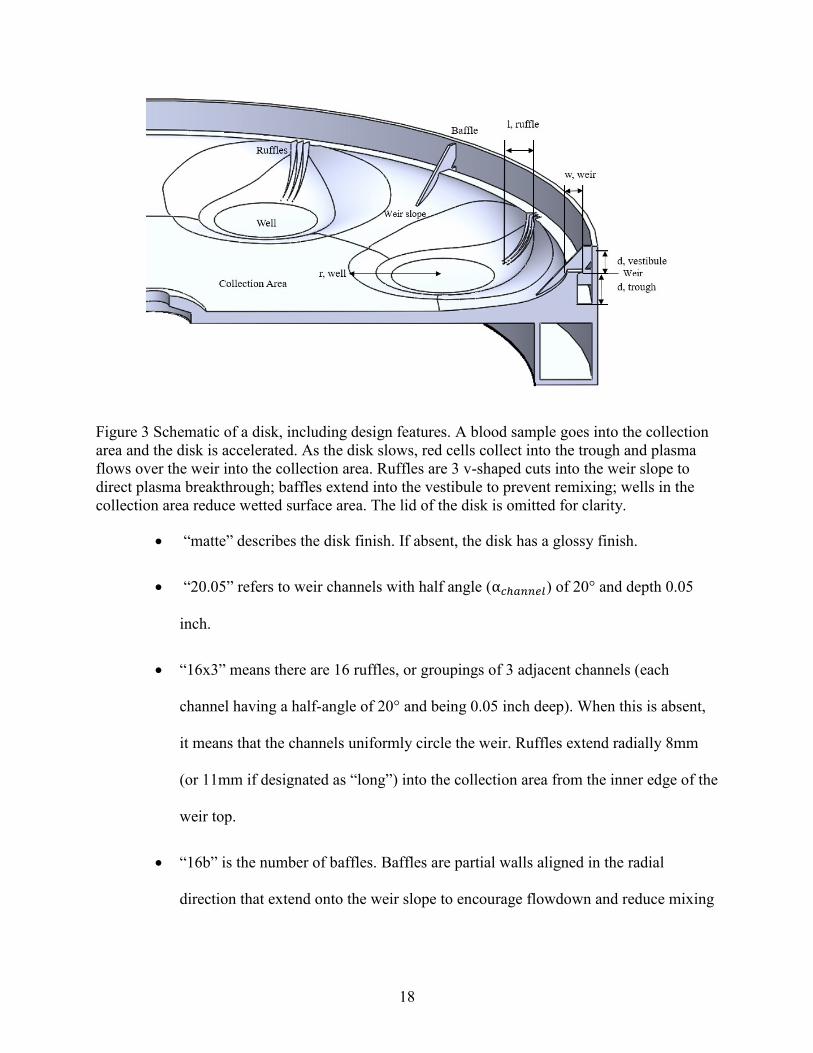
Figure 3 Schematic of a disk, including design features. A blood sample goes into the collection

area and the disk is accelerated. As the disk slows, red cells collect into the trough and plasma

flows over the weir into the collection area. Ruffles are 3 v-shaped cuts into the weir slope to

direct plasma breakthrough; baffles extend into the vestibule to prevent remixing; wells in the

collection area reduce wetted surface area. The lid of the disk is omitted for clarity.

• “matte” describes the disk finish. If absent, the disk has a glossy finish.

• “20.05” refers to weir channels with half angle (α𝑐ℎ𝑎𝑛𝑛𝑒𝑙) of 20° and depth 0.05

inch.

• “16x3” means there are 16 ruffles, or groupings of 3 adjacent channels (each

channel having a half-angle of 20° and being 0.05 inch deep). When this is absent,

it means that the channels uniformly circle the weir. Ruffles extend radially 8mm

(or 11mm if designated as “long”) into the collection area from the inner edge of the

weir top.

• “16b” is the number of baffles. Baffles are partial walls aligned in the radial

direction that extend onto the weir slope to encourage flowdown and reduce mixing

19

during spindown. They are from previous work. When channels and ruffles existed

in the same disk, they were evenly spaced apart (i.e. did not touch).

• “0.75x9mm” describes wells of depth 0.75mm and of radius 9mm cut into the

collection area at the end of a channel. The number of wells matches the number of

ruffles.

• “3mL” is the trough volume as measured from the bottom of the trough to the top of

the weir. If absent, the default trough volume is 4 mL.

• “peo” refers to a dried film of PEO (𝑀𝑣 = 100,000) on the weir.

Dimensions and volumes of the trough and vestibule were measured using intersections in

Solidworks. Table 5 in Appendix A shows selected dimensions.

3.2 Rapid prototyping

Rapid prototypes were 3D printed using a photocurable resin with a water-soluble support

material. (Stratasys Objet30 Prime). The body of a printed object is a stiff, cross-linked acrylate,

and printed features have a nominal resolution of 0.1 mm. This resin forms a smooth, translucent

surface, and is referred to as "glossy". If the printed object has body material that cannot be

directly supported by the body resin underneath, the printer uses a water-soluble support resin.

Removing the support resin requires at least power washing, but more extensive removal of

support requires soaking the whole object in aqueous 5-10 wt% NaOH solution for about 10

minutes. Even after extensive washing, support material can sometimes still be scratched off the

body surface. Consequently, objects that have not been reproducibly cleaned contain residual

support material. Any surface printed with the support materials is rough and opaque and is

referred to as “matte”, regardless of how clean it is. Immersing a printed object in a solvent for

20

longer than an hour caused the object to swell asymmetrically. This meant that disks could not be

soaked indefinitely to remove all support material from the trough.

3.3 Contact angle measurements

One-inch square wafers were printed with matte and glossy finishes. Glossy wafers

simulated hydrophobic polymers used in injection molding, such as polypropylene. Matte wafers

were printed to simulate the weir slopes of disks from previous work.

The contact angles of water and plasma were measured by placing a 2-4 μL drop on the

wafer surface deposited with a 10 μL Hamilton syringe and photographed with a goniometer

system (Sony Hyper HAD CCD-IRIS/RGB). Preliminary screening showed no convincing

evidence that drop size affected contact angle in these experiments, so the drop volume was

adjusted to maximize the drop size, while keeping the entire drop inside the camera field of view.

Contact angles were measured using the “Contact Angle” plugin for imageJ (developed by

Marco Brugnara).

Plasma proteins were coated onto the wafer surfaces to simulate the coating process that

occurs when blood is spun in the disk. In one method, 200 μL of plasma was pipetted onto a

wafer and removed after 1 minute. The remaining film was allowed to dry at room temperature

for 5-10 minutes. This is denoted as “air.dry10min”. In the second treatment, 200 μL of plasma

was pipetted onto a wafer over 20 seconds. Then, the wafer was blown on by a compressed air

jet for 3 minutes (the approximate duration of a spinning experiment) to remove excess plasma

and dry the wafer surface. This is referred to as “blown3min”. Third, a wafer was subjected to a

strong air jet as 200 μL of plasma was pipetted onto the surface along the edge. The plasma

immediately blew across the wafer, and the wafer stayed in the air jet for 1 minute. This is

21

referred to as “quick.dry”. After taking contact angle measurements on a coated wafer, the wafer

was scrubbed by hand with a wet Kimwipe and allowed to air dry. This is denoted as “wiped.”

3.4 Wafer experiments

The possibility of directing flowdown to specific locations is appealing because it gives

greater flexibility in designing future disks. Uniform flowdown is also desirable because it

distributes shear rate on the red cell pack around the whole disk, leading to less red cell

entrainment in the recovered plasma or essentially less red cell recovery. With this in mind, we

wanted to see if cutting v-shaped channels could create a wetted path for bulk plasma flow. Due

to the complex geometry of the disk weir, it was desirable to test the effect of channels in a

simplified scheme. The weir slope was approximated using 1 x 1 x 0.1 inch wafers printed with

v-shaped cutouts along 3/4 of the largest surface, as shown in Figure 4. A 0.25 x 1 inch region

was left bare to act as a reservoir. The reservoir and channels were separated by a v-shaped notch

perpendicular to the channels. The purpose of this notch was to prevent liquid contact with the

channels while to reservoir was being filled. The depth and angle of this notch were the same for

all wafers printed. Six wafers were printed with channel half-angles of 20, 50, and 70° and

depths of 0.025, and 0.05 inch. Two wafers were also printed without channels to serve as

controls. The first contained only the notch, and the second had a flat cut 0.05 inch in depth.

Each wafer's ID is the concatenation of the channel half angle and the depth. For example, a

wafer with 20° channels cut to 0.025 inch is referred to as "20.025". Wafers were printed with

matte and glossy finishes (as described above) and cleaned before use.

22

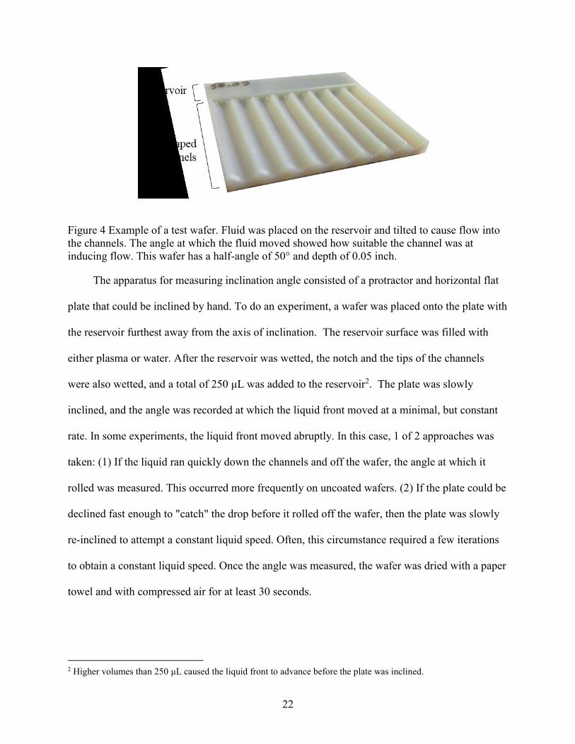
Figure 4 Example of a test wafer. Fluid was placed on the reservoir and tilted to cause flow into

the channels. The angle at which the fluid moved showed how suitable the channel was at

inducing flow. This wafer has a half-angle of 50° and depth of 0.05 inch.

The apparatus for measuring inclination angle consisted of a protractor and horizontal flat

plate that could be inclined by hand. To do an experiment, a wafer was placed onto the plate with

the reservoir furthest away from the axis of inclination. The reservoir surface was filled with

either plasma or water. After the reservoir was wetted, the notch and the tips of the channels

were also wetted, and a total of 250 μL was added to the reservoir2. The plate was slowly

inclined, and the angle was recorded at which the liquid front moved at a minimal, but constant

rate. In some experiments, the liquid front moved abruptly. In this case, 1 of 2 approaches was

taken: (1) If the liquid ran quickly down the channels and off the wafer, the angle at which it

rolled was measured. This occurred more frequently on uncoated wafers. (2) If the plate could be

declined fast enough to "catch" the drop before it rolled off the wafer, then the plate was slowly

re-inclined to attempt a constant liquid speed. Often, this circumstance required a few iterations

to obtain a constant liquid speed. Once the angle was measured, the wafer was dried with a paper

towel and with compressed air for at least 30 seconds.

2 Higher volumes than 250 μL caused the liquid front to advance before the plate was inclined.

23

3.4.1 Polymer coatings

To test the usefulness of hydrophilizing the weir with a polymer coating, the wafers were

independently coated with poly(acrylic acid) (PAA, Sigma-Aldrich, 𝑀𝑣 = 450,000) and

poly(ethylene oxide) (PEO, Sigma-Aldrich, 𝑀𝑣 = 100,000) dissolved in methanol3. PEO is only

lightly soluble in methanol (0.4 wt %), but more soluble when heated (3.4 wt % above 45 °C).

The wafer channels were coated with either a PAA or PEO solution using a foam brush. The

reservoir was not coated. Coated wafers were left to dry at room temperature for 10 min to 4

hours before measuring roll-down angles.

The inclination procedure of Section 3.4 was done with slight modification. After the angle

was measured, the water was spread along the channels using the side of the pipette tip and left

there for at least 10 seconds. Then, the wafer was dried for at least 30 s in compressed air and no

paper towel. This is referred to as 1 cycle. Subsequent cycles followed immediately.

3.5 Spinning experiments

3.5.1 Disk preparation and spinning

The support material had to be removed from the disks before use. For the wide, flat

surfaces of the disk, much of the support material could be scraped off. The trough and weir

were cleaned using a water jet at high pressure. This removed the bulk of the support but did not

remove support material on the disk surfaces. Matte disks were cleaned no further than this.

3 A brief investigation of solvents was done to screen for maximum volatility and minimal interaction with the disk

material. It was found that methylene chloride (NBP = 39.6 °C) and ethylene dichloride (NBP = 83.47 °C) extracted

low MW polymer from the disk material and a poly(propylene) (PP) sample. Acetone was found to asymmetrically

swell the printed material, leading to rotational instability. Eventually, methanol (NBP = 56 °C) was used because it

interacted with neither the printer material nor PP.

24

Glossy disks were cleaned further by filling the trough with a 5-10 wt% sodium hydroxide

solution for at least 10 minutes before re-spraying the trough with the water jet.

Residual support in the trough was problematic because it artifactually reduced the total

volume ~80-85% of the nominal trough volume for glossy disks. The real trough volume was

tested by placing the disk on a level surface and filling the trough until all the inner trough wall

was wetted. Once the disk is soaked in NaOH solution, the real volume increases to ~90% of the

nominal designed volume. This difference between real and nominal volume was not explicitly

tested for matte disks. However, the volume difference should be about twice as large in matte

disks because both the inner and the outer faces of the trough are printed with support material.4

In addition, the trough held 10-20% more than its nominal value (by of a meniscus) before the

liquid began to flow down the weir.

Each disk was prepared for spinning by rinsing it with tap water, drying off the excess

liquid with a paper towel, and using compressed air to remove water from the trough area. The

disk was secured onto a motor platform. After that, 7 mL of whole blood and 1.5 mL saline were

pipetted into collection area. These same volumes were used in all experiments unless otherwise

stated. The disk accelerated by 500 revolutions per minute (RPM) each second (RPM/s) until

3000 RPM, held that speed for 54 s (unless otherwise indicated), and then decelerated over ~2

minutes. Alizadeh et al. give a detailed spinning velocity profile [14]. Once the disk stopped, the

flowdown plasma was collected, weighed, and measured for hematocrit. Blood collected from

4 The printer can only print a glossy surface when there is no overhanging body. Previous (and continuing) work had

body material hanging over the inner edge of the trough, so this face had support material that needed to be

removed. Additionally, the disk lid hangs over the trough and weir, so glossy disks were printed without their lid,

and the lid was glued on after cleaning out the trough.

25

anonymous donors was refrigerated for no more than 24 hours and warmed to room temperature

before spinning.

3.5.2 Bacteria preparation and counting

Bacteria (E. coli: strain: BL21 DE3 star) were grown in nutrient broth overnight from a

streaked plate. The suspension was pelleted and resuspended in phosphate-buffered saline

(1xPBS) to give concentrations between 104 - 106 colony forming units (cfu) per mL. In

experiments using bacteria, 100 μL of this suspension (or 65 μL for dilution experiments where

the blood was diluted to hematocrit of 0.05 and 0.21) was spiked into equal volumes of PBS

(control) and PBS-diluted blood. The disk was filled with enough of this spiked blood mixture to

give a consistent fluid thickness of 3.3 mm. Table 5 (in Appendix A) shows the volumes of

whole blood-PBS suspension spun in the disk.

The collected plasma and the spiked PBS were diluted 1:9 in PBS and 50 μL of dilutions

10-2 through 10-5 were plated. Plates were incubated at 47 °C for 16+ hours and counted by hand.

Bacterial concentration recovery (see Section 3.5.3) was the ratio of bacterial concentrations in a

plasma sample divided by the average of bacterial concentration in the spiked PBS (called

control) for that set of experiments.

3.5.3 Definition of plasma, red cell and bacteria recoveries

Disk designs were evaluated by the fraction of the total plasma or red cells that flowed into

the collection area at the end of a spin. This section derives plasma, red cell, and bacteria

recovery from volume balances. Experiments that focused on disk designs did not use bacteria,

so plasma recovery is a surrogate value for bacteria recovery. This derivation is more precise

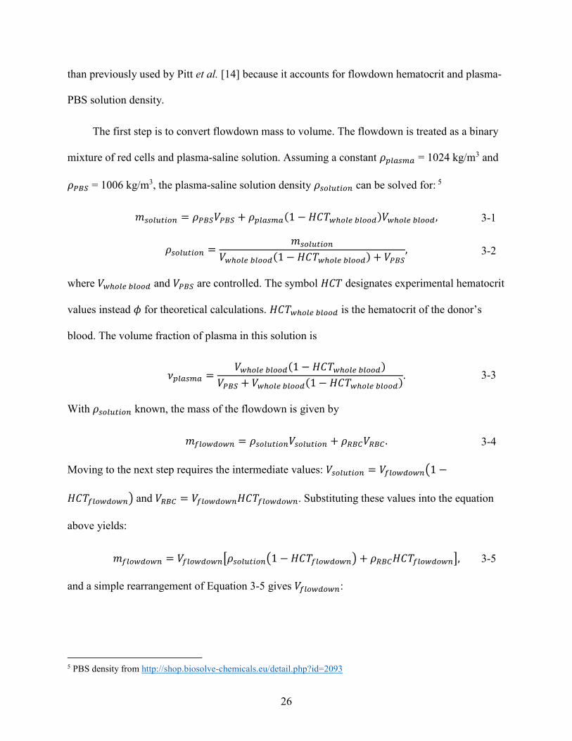
26

than previously used by Pitt et al. [14] because it accounts for flowdown hematocrit and plasma-

PBS solution density.

The first step is to convert flowdown mass to volume. The flowdown is treated as a binary

mixture of red cells and plasma-saline solution. Assuming a constant 𝜌𝑝𝑙𝑎𝑠𝑚𝑎 = 1024 kg/m3 and

𝜌𝑃𝐵𝑆 = 1006 kg/m3, the plasma-saline solution density 𝜌𝑠𝑜𝑙𝑢𝑡𝑖𝑜𝑛 can be solved for: 5

𝑚𝑠𝑜𝑙𝑢𝑡𝑖𝑜𝑛 = 𝜌𝑃𝐵𝑆𝑉𝑃𝐵𝑆 + 𝜌𝑝𝑙𝑎𝑠𝑚𝑎(1 − 𝐻𝐶𝑇𝑤ℎ𝑜𝑙𝑒 𝑏𝑙𝑜𝑜𝑑)𝑉𝑤ℎ𝑜𝑙𝑒 𝑏𝑙𝑜𝑜𝑑, 3-1

𝜌𝑠𝑜𝑙𝑢𝑡𝑖𝑜𝑛 =𝑚𝑠𝑜𝑙𝑢𝑡𝑖𝑜𝑛

𝑉𝑤ℎ𝑜𝑙𝑒 𝑏𝑙𝑜𝑜𝑑(1 − 𝐻𝐶𝑇𝑤ℎ𝑜𝑙𝑒 𝑏𝑙𝑜𝑜𝑑) + 𝑉𝑃𝐵𝑆, 3-2

where 𝑉𝑤ℎ𝑜𝑙𝑒 𝑏𝑙𝑜𝑜𝑑 and 𝑉𝑃𝐵𝑆 are controlled. The symbol 𝐻𝐶𝑇 designates experimental hematocrit

values instead 𝜙 for theoretical calculations. 𝐻𝐶𝑇𝑤ℎ𝑜𝑙𝑒 𝑏𝑙𝑜𝑜𝑑 is the hematocrit of the donor’s

blood. The volume fraction of plasma in this solution is

𝜈𝑝𝑙𝑎𝑠𝑚𝑎 =

𝑉𝑤ℎ𝑜𝑙𝑒 𝑏𝑙𝑜𝑜𝑑(1 − 𝐻𝐶𝑇𝑤ℎ𝑜𝑙𝑒 𝑏𝑙𝑜𝑜𝑑)

𝑉𝑃𝐵𝑆 + 𝑉𝑤ℎ𝑜𝑙𝑒 𝑏𝑙𝑜𝑜𝑑(1 − 𝐻𝐶𝑇𝑤ℎ𝑜𝑙𝑒 𝑏𝑙𝑜𝑜𝑑). 3-3

With 𝜌𝑠𝑜𝑙𝑢𝑡𝑖𝑜𝑛 known, the mass of the flowdown is given by

𝑚𝑓𝑙𝑜𝑤𝑑𝑜𝑤𝑛 = 𝜌𝑠𝑜𝑙𝑢𝑡𝑖𝑜𝑛𝑉𝑠𝑜𝑙𝑢𝑡𝑖𝑜𝑛 + 𝜌𝑅𝐵𝐶𝑉𝑅𝐵𝐶 . 3-4

Moving to the next step requires the intermediate values: 𝑉𝑠𝑜𝑙𝑢𝑡𝑖𝑜𝑛 = 𝑉𝑓𝑙𝑜𝑤𝑑𝑜𝑤𝑛(1 −

𝐻𝐶𝑇𝑓𝑙𝑜𝑤𝑑𝑜𝑤𝑛) and 𝑉𝑅𝐵𝐶 = 𝑉𝑓𝑙𝑜𝑤𝑑𝑜𝑤𝑛𝐻𝐶𝑇𝑓𝑙𝑜𝑤𝑑𝑜𝑤𝑛. Substituting these values into the equation

above yields:

𝑚𝑓𝑙𝑜𝑤𝑑𝑜𝑤𝑛 = 𝑉𝑓𝑙𝑜𝑤𝑑𝑜𝑤𝑛[𝜌𝑠𝑜𝑙𝑢𝑡𝑖𝑜𝑛(1 − 𝐻𝐶𝑇𝑓𝑙𝑜𝑤𝑑𝑜𝑤𝑛) + 𝜌𝑅𝐵𝐶𝐻𝐶𝑇𝑓𝑙𝑜𝑤𝑑𝑜𝑤𝑛], 3-5

and a simple rearrangement of Equation 3-5 gives 𝑉𝑓𝑙𝑜𝑤𝑑𝑜𝑤𝑛:

5 PBS density from http://shop.biosolve-chemicals.eu/detail.php?id=2093

27

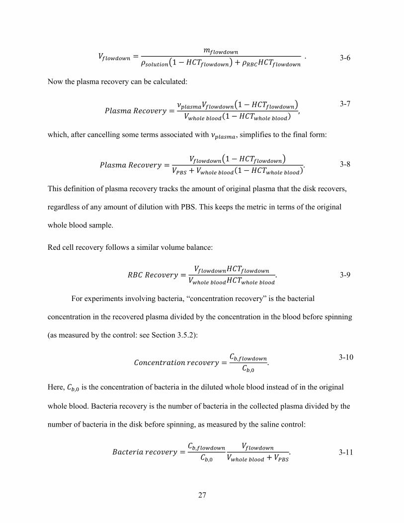
𝑉𝑓𝑙𝑜𝑤𝑑𝑜𝑤𝑛 =𝑚𝑓𝑙𝑜𝑤𝑑𝑜𝑤𝑛

𝜌𝑠𝑜𝑙𝑢𝑡𝑖𝑜𝑛(1 − 𝐻𝐶𝑇𝑓𝑙𝑜𝑤𝑑𝑜𝑤𝑛) + 𝜌𝑅𝐵𝐶𝐻𝐶𝑇𝑓𝑙𝑜𝑤𝑑𝑜𝑤𝑛

. 3-6

Now the plasma recovery can be calculated:

𝑃𝑙𝑎𝑠𝑚𝑎 𝑅𝑒𝑐𝑜𝑣𝑒𝑟𝑦 =

𝜈𝑝𝑙𝑎𝑠𝑚𝑎𝑉𝑓𝑙𝑜𝑤𝑑𝑜𝑤𝑛(1 − 𝐻𝐶𝑇𝑓𝑙𝑜𝑤𝑑𝑜𝑤𝑛)

𝑉𝑤ℎ𝑜𝑙𝑒 𝑏𝑙𝑜𝑜𝑑(1 − 𝐻𝐶𝑇𝑤ℎ𝑜𝑙𝑒 𝑏𝑙𝑜𝑜𝑑),

3-7

which, after cancelling some terms associated with 𝜈𝑝𝑙𝑎𝑠𝑚𝑎, simplifies to the final form:

𝑃𝑙𝑎𝑠𝑚𝑎 𝑅𝑒𝑐𝑜𝑣𝑒𝑟𝑦 =

𝑉𝑓𝑙𝑜𝑤𝑑𝑜𝑤𝑛(1 − 𝐻𝐶𝑇𝑓𝑙𝑜𝑤𝑑𝑜𝑤𝑛)

𝑉𝑃𝐵𝑆 + 𝑉𝑤ℎ𝑜𝑙𝑒 𝑏𝑙𝑜𝑜𝑑(1 − 𝐻𝐶𝑇𝑤ℎ𝑜𝑙𝑒 𝑏𝑙𝑜𝑜𝑑). 3-8

This definition of plasma recovery tracks the amount of original plasma that the disk recovers,

regardless of any amount of dilution with PBS. This keeps the metric in terms of the original

whole blood sample.

Red cell recovery follows a similar volume balance:

𝑅𝐵𝐶 𝑅𝑒𝑐𝑜𝑣𝑒𝑟𝑦 =

𝑉𝑓𝑙𝑜𝑤𝑑𝑜𝑤𝑛𝐻𝐶𝑇𝑓𝑙𝑜𝑤𝑑𝑜𝑤𝑛

𝑉𝑤ℎ𝑜𝑙𝑒 𝑏𝑙𝑜𝑜𝑑𝐻𝐶𝑇𝑤ℎ𝑜𝑙𝑒 𝑏𝑙𝑜𝑜𝑑. 3-9

For experiments involving bacteria, “concentration recovery” is the bacterial

concentration in the recovered plasma divided by the concentration in the blood before spinning

(as measured by the control: see Section 3.5.2):

𝐶𝑜𝑛𝑐𝑒𝑛𝑡𝑟𝑎𝑡𝑖𝑜𝑛 𝑟𝑒𝑐𝑜𝑣𝑒𝑟𝑦 =

𝐶𝑏,𝑓𝑙𝑜𝑤𝑑𝑜𝑤𝑛

𝐶𝑏,0.

3-10

Here, 𝐶𝑏,0 is the concentration of bacteria in the diluted whole blood instead of in the original

whole blood. Bacteria recovery is the number of bacteria in the collected plasma divided by the

number of bacteria in the disk before spinning, as measured by the saline control:

𝐵𝑎𝑐𝑡𝑒𝑟𝑖𝑎 𝑟𝑒𝑐𝑜𝑣𝑒𝑟𝑦 =

𝐶𝑏,𝑓𝑙𝑜𝑤𝑑𝑜𝑤𝑛

𝐶𝑏,0

𝑉𝑓𝑙𝑜𝑤𝑑𝑜𝑤𝑛

𝑉𝑤ℎ𝑜𝑙𝑒 𝑏𝑙𝑜𝑜𝑑 + 𝑉𝑃𝐵𝑆. 3-11

28

3.6 Statistics

Statistical hypothesis tests were chosen for how appropriately the data met the model

assumptions. Two-sample or paired t-tests were used when applicable, but non-parametric rank

tests were used when these assumptions were not satisfied, such as for RBC recovery where

values may not decrease below 0. Data and code for all statistical analyses can be found in the

“data-analysis” folder in the github repository (https://github.com/cliffanderson720/MS-Thesis-

Pitt). Statistical analysis and figures involving experimental data were done using the R

programming language.

A note on experimental design: surprising variability exists between blood samples from

different donors. See Section 5.2. However, blocking and randomization of blood samples for

most disk design experiments were haphazard or nonexistent for early experiments, unless

otherwise specified. In these cases, efforts at blocking and randomization are detailed.

Experimental values are reported as mean and standard deviation unless otherwise noted.

Regressions are fitted using a least-squares procedure, and points were discarded if their

Studentized residuals exceeded 2.

29

4 EXPERIMENTAL RESULTS AND DISCUSSION OF DISK DESIGNS

This chapter describes disk modifications and their effects on breakthrough, plasma recovery,

and red cell recovery. It first describes general surface properties of the disk material, followed

by exploratory experiments aimed at inducing capillary flow. The remainder of the chapter

focuses on disk modifications that were informed by past work and ongoing findings. Specific

recommendations are postponed until Chapter 6.

4.1 Contact angle

We observed that disk material wetted more easily after it had been coated with a film of

dried blood. Wettability is desirable, but the extent to which the weir surface was affected by

contact with the blood was unknown. Vroman showed that small proteins, such as antibodies,

adhere rapidly to surfaces and are eventually displaced by proteins with greater affinity for the

surface [53]. The affinity of blood proteins is strong enough that solvents alone cannot remove

them [54]. Furthermore, studies on plasma protein adsorption onto polymeric surfaces suggest

that adsorbing proteins such as albumin, globulin, fibrinogen, or IgG orient their most polar

regions toward a polar surface [55]. Consequently, the more hydrophobic regions of a protein

orient toward the disk surface, leaving hydrophilic ends oriented towards the air, which makes

the surface more wettable to water. In this section, we investigated the effect of plasma exposure

30

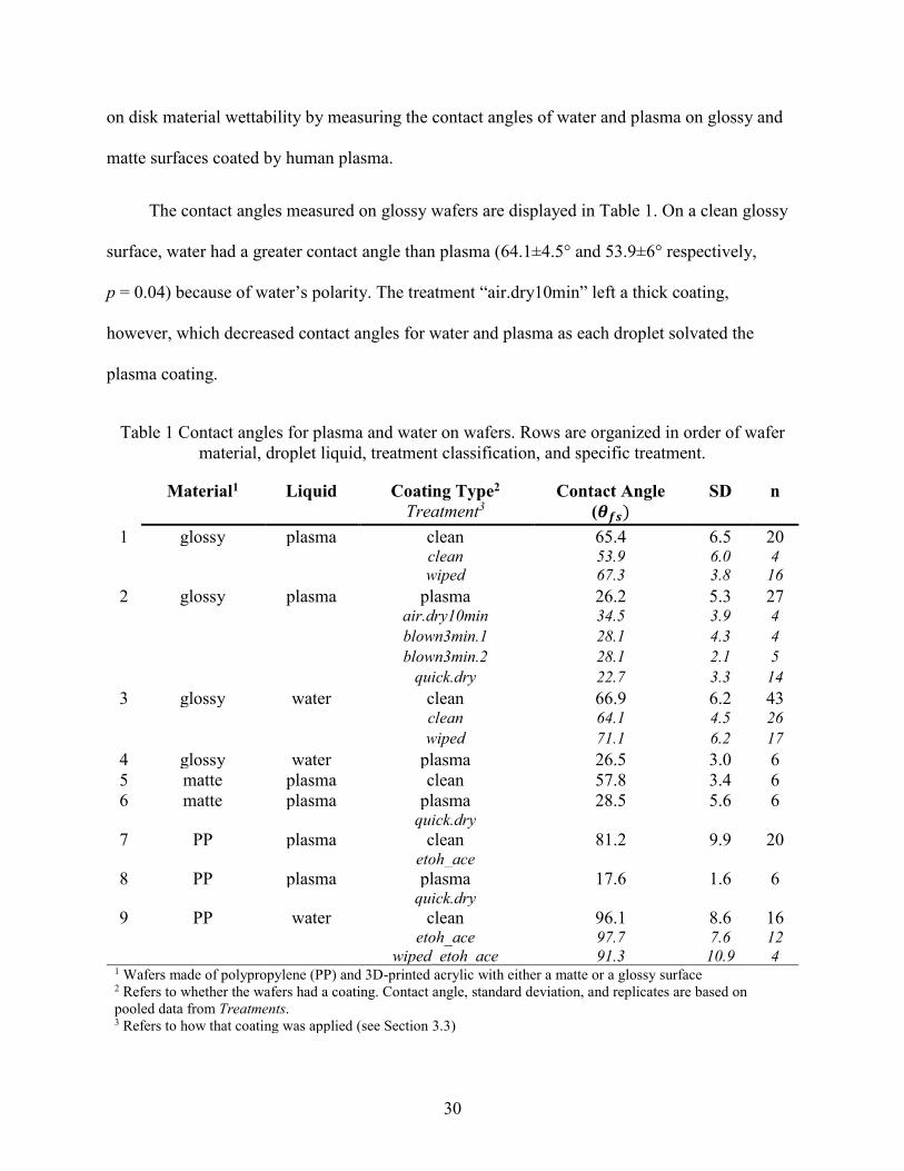
on disk material wettability by measuring the contact angles of water and plasma on glossy and

matte surfaces coated by human plasma.

The contact angles measured on glossy wafers are displayed in Table 1. On a clean glossy

surface, water had a greater contact angle than plasma (64.1±4.5° and 53.9±6° respectively,

p = 0.04) because of water’s polarity. The treatment “air.dry10min” left a thick coating,

however, which decreased contact angles for water and plasma as each droplet solvated the

plasma coating.

Table 1 Contact angles for plasma and water on wafers. Rows are organized in order of wafer

material, droplet liquid, treatment classification, and specific treatment.

Material1 Liquid Coating Type2 Contact Angle SD n

Treatment3 (𝜽𝒇𝒔)

1 glossy plasma clean 65.4 6.5 20 clean 53.9 6.0 4

wiped 67.3 3.8 16

2 glossy plasma plasma 26.2 5.3 27

air.dry10min 34.5 3.9 4

blown3min.1 28.1 4.3 4

blown3min.2 28.1 2.1 5

quick.dry 22.7 3.3 14

3 glossy water clean 66.9 6.2 43

clean 64.1 4.5 26

wiped 71.1 6.2 17

4 glossy water plasma 26.5 3.0 6

5 matte plasma clean 57.8 3.4 6

6 matte plasma plasma 28.5 5.6 6 quick.dry

7 PP plasma clean 81.2 9.9 20 etoh_ace

8 PP plasma plasma 17.6 1.6 6 quick.dry

9 PP water clean 96.1 8.6 16 etoh_ace 97.7 7.6 12

wiped_etoh_ace 91.3 10.9 4 1 Wafers made of polypropylene (PP) and 3D-printed acrylic with either a matte or a glossy surface 2 Refers to whether the wafers had a coating. Contact angle, standard deviation, and replicates are based on

pooled data from Treatments. 3 Refers to how that coating was applied (see Section 3.3)

31

To more accurately replicate the short plasma-surface contact time in a spinning

experiment, treatment “blown3min” was applied and found to maintain a low contact angle

(28.1°) for two repetitions. Removing the dried plasma film with a wet Kimwipe raised the

contact angles of water (71.1±6.2°) and plasma (53.9±6°) above those on the original clean

surface (p < 0.05 for two-sample t-test between “clean” and “wiped” for both plasma and water),

indicating that the plasma coating may be removed from a disk through mechanical abrasion.

Treatment “blown3min” gave a qualitatively thinner coating than “air.dry10min” but seemed to

over-estimate the contact time experienced in an actual spinning experiment. Treatment

“quick.dry” did not leave a film of visible thickness, but its contact angle remained low

(23.4±3.9°). This indicates that short contact times with plasma are sufficient to increase the

wettability of a hydrophobic surface.

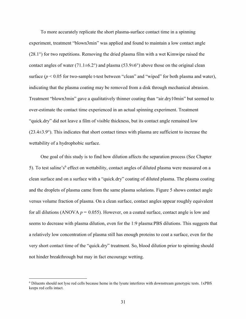
One goal of this study is to find how dilution affects the separation process (See Chapter

5). To test saline’s6 effect on wettability, contact angles of diluted plasma were measured on a

clean surface and on a surface with a “quick.dry” coating of diluted plasma. The plasma coating

and the droplets of plasma came from the same plasma solutions. Figure 5 shows contact angle

versus volume fraction of plasma. On a clean surface, contact angles appear roughly equivalent

for all dilutions (ANOVA p = 0.055). However, on a coated surface, contact angle is low and

seems to decrease with plasma dilution, even for the 1:9 plasma:PBS dilutions. This suggests that

a relatively low concentration of plasma still has enough proteins to coat a surface, even for the

very short contact time of the “quick.dry” treatment. So, blood dilution prior to spinning should

not hinder breakthrough but may in fact encourage wetting.

6 Diluents should not lyse red cells because heme in the lysate interferes with downstream genotypic tests. 1xPBS

keeps red cells intact.

32

Figure 5 Contact angle of plasma-saline dilutions on plasma-coated 3D printed wafers. Wafers

coated with diluted plasma (“quick.dry” treatment) are very hydrophilic, even when plasma is

diluted 1:9 with saline.

Uniform flowdown after deceleration may return clearer plasma by reducing shear at the

plasma-cell pack interface. During deceleration, the plasma is pulled down by gravity, but is

prevented from advancing down the weir by the work required to wet the weir surface. Instead,

the liquid bulges near the wetting line until breakthrough, where increasing hydrostatic pressure

finally overcomes the wetting resistance. Breakthrough can be abrupt and entrain red cells from

the sediment layer. Often, the plasma flows down the weir slope in 1 to 3 locations, providing a

wetted surface for the rest of the plasma to flow over down into the collecting area. It’s possible

that a hydrophilic weir surface may present a smaller surface energy barrier, permitting more

uniform flowdown and less entrainment of RBCs. The data in Figure 5 also indicate that a

plasma coating does not affect wettability for matte as much as for glossy. Glossy surfaces are

preferable because the data statistically verified that they had more uniform flowdown and faster

breakthrough (see Section 4.3.1).

33

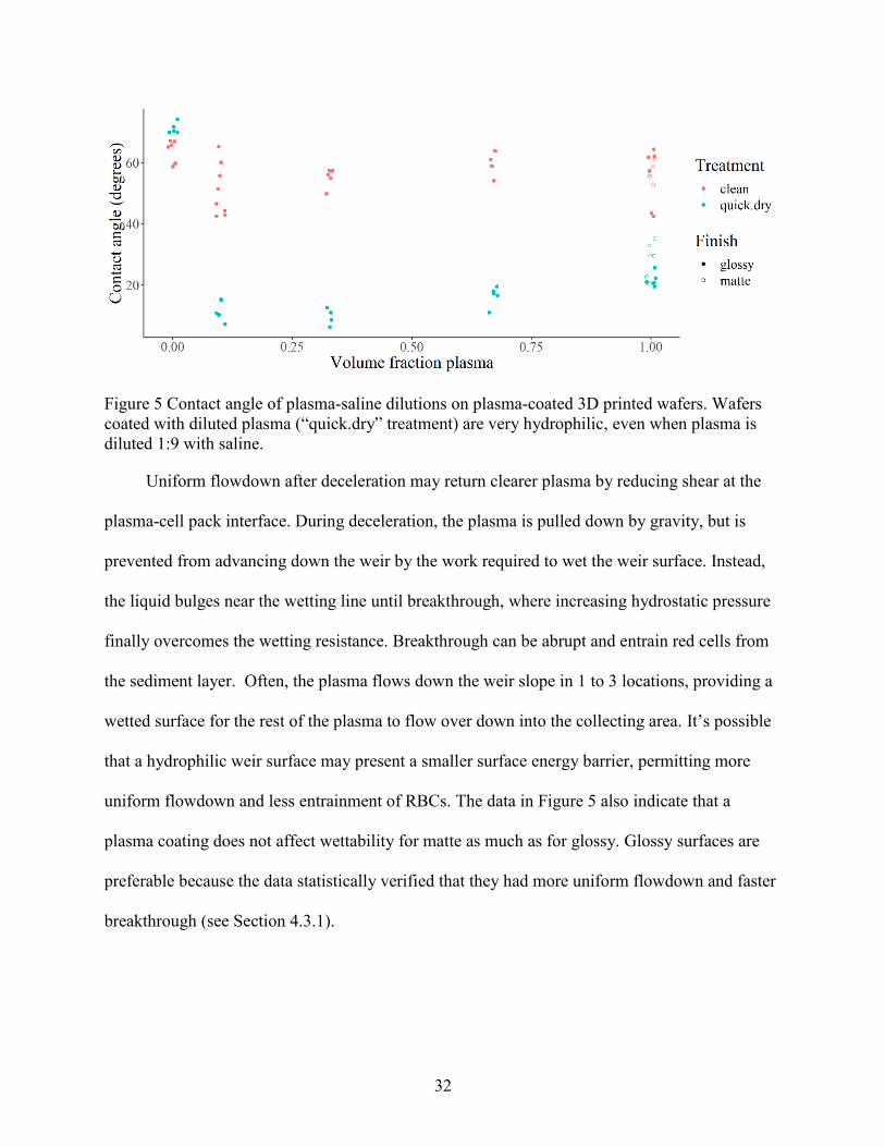
4.2 Liquids on tilted wafers

To test the effects on breakthrough that might be caused by cutting channels into the weir, we

prototyped wafers with v-shaped channels of varied half-angles (α𝑐ℎ𝑎𝑛𝑛𝑒𝑙 ∈ [20,50,70∘]) and

depths (0.0, 0.025, 0.05 inch) and measured how much the wafer needed to tilt before the liquid

would flow down the surface. Each wafer's ID is the concatenation of the channel half angle and

the depth. Inclination angles for water on glossy wafers coated with PEO are shown in Figure 6.

The inclination angle was the lowest for freshly PEO-coated wafers, and some channels wetted

spontaneously7. The inclination angle reached a steady value with repeated cycles as the PEO

washed off. Final inclination angles decreased with channel half-angle for 0.025 inch channels,

indicating that narrow channels provide less resistance to wetting. Narrower channels also took

longer to reach their final angle, suggesting that narrow channels retained the PEO better.

Figure 6 Summary of PEO coating effect on inclination angles for consecutive cycles (n=4, SE

shown). Each wafer with the PEO coating wetted easily. As the experiment was repeated, the

polymer washed off, and the angle at which the fluid steadily moved down the channels

increased to a steady value. The hydrophilic PEO coating washed off for all wafers except 20.05.

7 A few experiments using plasma as the liquid also wetted spontaneously

34

At a depth of 0.05 inch, this trend is less clear. What is of special note, however, is that

the wafer 20.05 wicked water from the reservoir down the channels for every cycle. Due to the

sharp wedge geometry, perhaps solvated PEO remained in the channels’ bottoms despite the

water removal after each cycle. This means that the 20.05 channels reliably wick water, even if

the hydrophilic coating is compromised. The 20.025 wafer also wicked water down the channels,

but these inclination angle experiments only measured bulk flow down the wafer. This was

intentional because when breakthrough happens on a disk, the plasma flows down in bulk rather

than purely by capillary flow.

In order to understand these results, Berthier gives an inequality to predict spontaneous

capillary flow in v-shaped open channels (Equation 4-1) (see pg 40 Table 1.1 of ref [56]):

𝑤

2𝑑< 𝑐𝑜𝑠 𝜃𝑓𝑠. 4-1

Here, 𝑤 is the peak-to-peak channel width, 𝑑 is slant height, or trough-to-peak distance, and 𝜃𝑓𝑠

is the fluid-solid contact angle. Spontaneous capillary flows occur when this inequality holds.

Using the identity 𝑤/2

𝑑= 𝑠𝑖𝑛 𝛼𝑐ℎ𝑎𝑛𝑛𝑒𝑙, Equation 4-1 becomes

𝑠𝑖𝑛 𝛼𝑐ℎ𝑎𝑛𝑛𝑒𝑙 < 𝑐𝑜𝑠 𝜃𝑓𝑠 , 4-2

where 𝛼𝑐ℎ𝑎𝑛𝑛𝑒𝑙 is the channel half-angle. The same inequality in slightly less trigonometric form

reads:

90 − 𝛼𝑐ℎ𝑎𝑛𝑛𝑒𝑙 < 𝜃𝑓𝑠, 𝛼𝑐ℎ𝑎𝑛𝑛𝑒𝑙 ∈ [0,90]. 4-3

According to this theory, a contact angle lower than 70° is sufficient to cause SCF in a 20°

channel. Thus, broad channels may induce SCF for an extremely wettable surface (i.e. 𝜃𝑓𝑠 tends

35

to 0°) but may not induce anything if the surface becomes less wettable. This theory supports the

wicking observed in 20° channels and can guide future work in creating capillary flow.

4.3 Disk weir design

This section defines disk features and describes weir modifications and their effect on

breakthrough. Specific effects on plasma and red cell recoveries are discussed in Sections 4.5

and 4.6. The reader is encouraged to review disk features shown in Figure 3 before continuing.

4.3.1 Glossy

Replacing the matte finish with a glossy finish reduces the within-disk standard deviation

of volumetric flowdown by 67% (54-76 95% confidence, 𝐹0.975,128,29). Plasma-coated glossy and

matte surfaces have similar contact angles (22.7°±3.3 vs 28.5°±5.6 p = 0.053), so contact angle

alone does not explain the difference. Rather, it may be the presence of unremoved support

material. Support material can be easily removed from a flat surface, but weir slopes and

modifications, such as ruffle and baffles, are difficult to clean.

4.3.2 Ruffles

The capillary flow results from the 20.05 wafer suggested that channels cut into the weir

could induce breakthrough in predetermined spots. Disks were printed with 16 ruffles, or

groupings of 3 contiguous channels, cut into the weir to induce breakthrough by capillary flow.

As a disk decelerated below ~100 RPM, beads of plasma initiated by the ruffles appear on the

top weir edge and usually broke through in 2-7 out of 16 places (See Figure 8 for an example).

36

16 ruffles were chosen to evenly compare to disks containing 16 baffles, but the breakthrough

occurs qualitatively the same for disks with 8 ruffles8.

On disks with 16 ruffles, the ruffles were cut to full depth (0.05 inch) at the weir top, but

they grew shallower as they descended into the collection area. This was problematic because

shallow channels do not wet as easily as deeper ones (See Section 4.2). On disks with 8 ruffles,

we extended the ruffles further into the collection area (from 8 mm to 11 mm), which allowed

the channels to cut deeply into the weir for a greater distance along the weir slope before

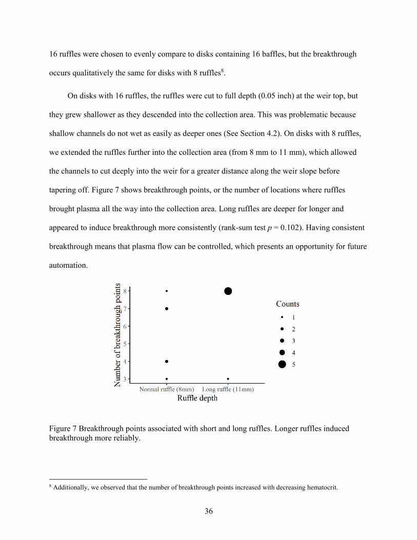
tapering off. Figure 7 shows breakthrough points, or the number of locations where ruffles

brought plasma all the way into the collection area. Long ruffles are deeper for longer and

appeared to induce breakthrough more consistently (rank-sum test p = 0.102). Having consistent

breakthrough means that plasma flow can be controlled, which presents an opportunity for future

automation.

Figure 7 Breakthrough points associated with short and long ruffles. Longer ruffles induced

breakthrough more reliably.

8 Additionally, we observed that the number of breakthrough points increased with decreasing hematocrit.

37

The spontaneous capillary flow (SCF) theory does not explain everything though. Matte

contact angles for plasma-coated surfaces (𝜃𝑓𝑠 = 28.5°) predict capillary flow for

𝜙𝑐ℎ𝑎𝑛𝑛𝑒𝑙 < 61.5°. However, SCF never occurred on breakthrough for any matte disks with

ruffles9.

4.3.3 Wells

The plasma film that remains on a glossy surface after pipetting up the bulk fluid has a

mass of 3.72 mg/cm2 (±0.23 95% confidence) of plasma-wetted surface. On an average spin, the

wetted area is about 25 cm2, so about 0.1g (up to 5% of the total plasma) of the flowdown is

unrecoverable by pipetting. We reduced wetted surface area in a disk by cutting wells into the

collection area so that plasma could bead up. For these experiments, breakthrough occurred

solely into the wells for 32 out of 34 experimental spins. The ruffles generated breakthrough and

the wells controlled where plasma flowed. Less reliable, however, were the number of

breakthrough points and of wells that actually filled up with plasma. A typical spin had 3-7

breakthrough points, and 1-3 fully filled wells. Diluted blood, however, consistently had 8

evenly filled wells, although none were full. This suggests that the breakthrough location of

diluted blood may be easier to direct, perhaps because of lower viscosity or higher surface

tension.

Examples of flowdown on each type of disk are shown in Figure 8.

9 Residual support material in the channels did not always dry completely between spins. Blood in the collection

area in preparation for the next spin occasionally wicked up the channels. This was fun to watch.

38

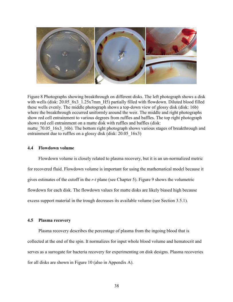
Figure 8 Photographs showing breakthrough on different disks. The left photograph shows a disk

with wells (disk: 20.05_8x3_1.25x7mm_H5) partially filled with flowdown. Diluted blood filled

these wells evenly. The middle photograph shows a top-down view of glossy disk (disk: 16b)

where the breakthrough occurred uniformly around the weir. The middle and right photographs

show red cell entrainment to various degrees from ruffles and baffles. The top right photograph

shows red cell entrainment on a matte disk with ruffles and baffles (disk:

matte_70.05_16x3_16b). The bottom right photograph shows various stages of breakthrough and

entrainment due to ruffles on a glossy disk (disk: 20.05_16x3)

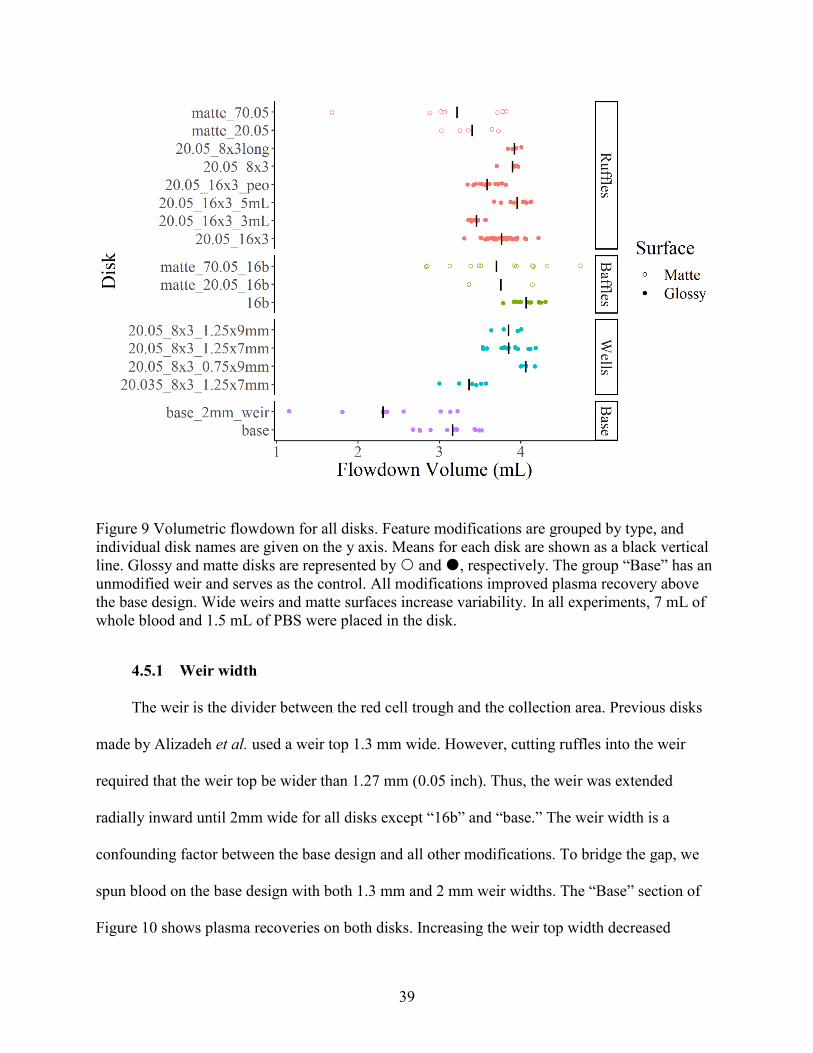
4.4 Flowdown volume

Flowdown volume is closely related to plasma recovery, but it is an un-normalized metric

for recovered fluid. Flowdown volume is important for using the mathematical model because it

gives estimates of the cutoff in the r-t plane (see Chapter 5). Figure 9 shows the volumetric

flowdown for each disk. The flowdown values for matte disks are likely biased high because

excess support material in the trough decreases its available volume (see Section 3.5.1).

4.5 Plasma recovery

Plasma recovery describes the percentage of plasma from the ingoing blood that is

collected at the end of the spin. It normalizes for input whole blood volume and hematocrit and

serves as a surrogate for bacteria recovery for experimenting on disk designs. Plasma recoveries

for all disks are shown in Figure 10 (also in Appendix A).

39

Figure 9 Volumetric flowdown for all disks. Feature modifications are grouped by type, and

individual disk names are given on the y axis. Means for each disk are shown as a black vertical

line. Glossy and matte disks are represented by and , respectively. The group “Base” has an

unmodified weir and serves as the control. All modifications improved plasma recovery above

the base design. Wide weirs and matte surfaces increase variability. In all experiments, 7 mL of

whole blood and 1.5 mL of PBS were placed in the disk.

4.5.1 Weir width

The weir is the divider between the red cell trough and the collection area. Previous disks

made by Alizadeh et al. used a weir top 1.3 mm wide. However, cutting ruffles into the weir

required that the weir top be wider than 1.27 mm (0.05 inch). Thus, the weir was extended

radially inward until 2mm wide for all disks except “16b” and “base.” The weir width is a

confounding factor between the base design and all other modifications. To bridge the gap, we

spun blood on the base design with both 1.3 mm and 2 mm weir widths. The “Base” section of

Figure 10 shows plasma recoveries on both disks. Increasing the weir top width decreased

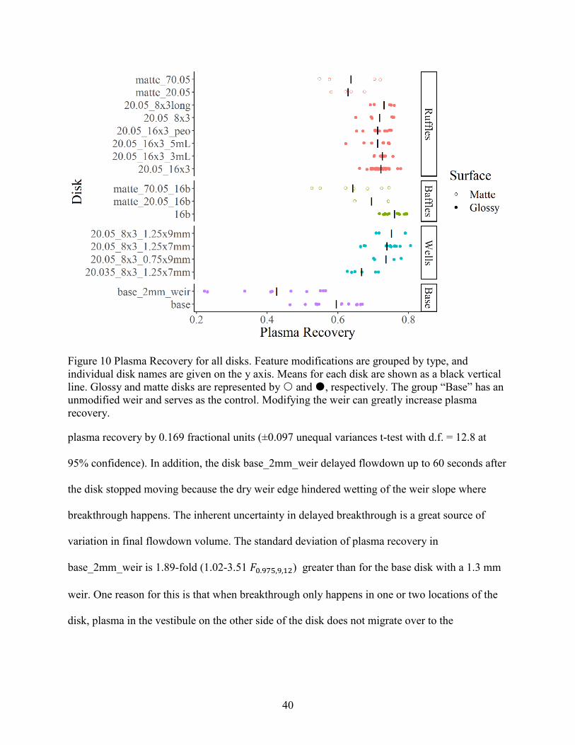
40

Figure 10 Plasma Recovery for all disks. Feature modifications are grouped by type, and

individual disk names are given on the y axis. Means for each disk are shown as a black vertical

line. Glossy and matte disks are represented by and , respectively. The group “Base” has an

unmodified weir and serves as the control. Modifying the weir can greatly increase plasma

recovery.

plasma recovery by 0.169 fractional units (±0.097 unequal variances t-test with d.f. = 12.8 at

95% confidence). In addition, the disk base_2mm_weir delayed flowdown up to 60 seconds after

the disk stopped moving because the dry weir edge hindered wetting of the weir slope where

breakthrough happens. The inherent uncertainty in delayed breakthrough is a great source of

variation in final flowdown volume. The standard deviation of plasma recovery in

base_2mm_weir is 1.89-fold (1.02-3.51 𝐹0.975,9,12) greater than for the base disk with a 1.3 mm

weir. One reason for this is that when breakthrough only happens in one or two locations of the

disk, plasma in the vestibule on the other side of the disk does not migrate over to the

41

breakthrough point to flow down. The longer breakthrough takes to happen, the more likely it is

that it will only happen in one place, and hence that there will be more unrecovered plasma.

Even in disks having consistent breakthrough, the trough/vestibule area holds more fluid

than the designed trough volume (see Section 3.5.1). A brief experiment indicates this volume is

0.88 mL (±0.15 95% confidence) for a 1:9 plasma:PBS solution on a disk with a shallow trough

(volume: 0.37 mL, disk: 20.05_8x3_1.25x7mm_H5). Observations show that a meniscus forms

between the weir top and the back wall. Changing the weir width tests the hypothesis that the

unrecovered fluid is comprised of the meniscus. Making the weir wider should increase the

volume of the meniscus (assuming that wetting angle is constant with geometry), trapping more

plasma in the vestibule and reducing plasma recovery. The decreased plasma recovery associated

with the wider weir supports this hypothesis. Future work could focus on reducing the meniscus

volume because it constitutes up to 30% of the original plasma volume.

4.5.2 Effect of weir slope designs

Figure 10 shows plasma recovery for all disks, grouped by modification type. A clear

difference exists between disks with modified and unmodified weir slopes. Specifically, the

presence of baffles on the base disk increased plasma recovery by 0.164 fractional units (±0.043

95% confidence) more than for base. Ruffles and wells increased plasma recovery by 0.294

fractional units (±0.092 95% confidence) and 0.314 fractional units (±0.093 95% confidence)

more than base_2mm_weir, respectively. Adding ruffles (and wells) to the 2 mm weir provides a

pre-wetted breakthrough point for the plasma and reduces variability in plasma recovery.

Although ruffles and wells improved plasma recovery much more than baffles did, they also

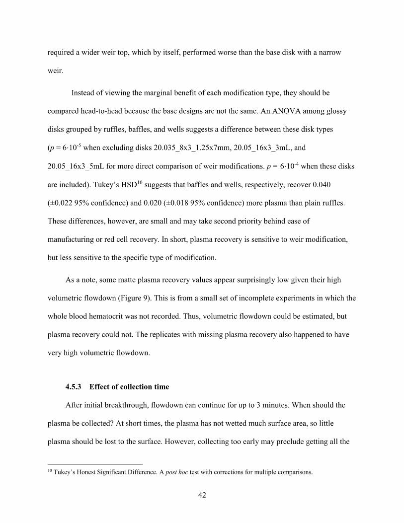
42

required a wider weir top, which by itself, performed worse than the base disk with a narrow

weir.

Instead of viewing the marginal benefit of each modification type, they should be

compared head-to-head because the base designs are not the same. An ANOVA among glossy

disks grouped by ruffles, baffles, and wells suggests a difference between these disk types

(p = 6⋅10-5 when excluding disks 20.035_8x3_1.25x7mm, 20.05_16x3_3mL, and

20.05_16x3_5mL for more direct comparison of weir modifications. p = 6⋅10-4 when these disks

are included). Tukey’s HSD10 suggests that baffles and wells, respectively, recover 0.040

(±0.022 95% confidence) and 0.020 (±0.018 95% confidence) more plasma than plain ruffles.

These differences, however, are small and may take second priority behind ease of

manufacturing or red cell recovery. In short, plasma recovery is sensitive to weir modification,

but less sensitive to the specific type of modification.

As a note, some matte plasma recovery values appear surprisingly low given their high

volumetric flowdown (Figure 9). This is from a small set of incomplete experiments in which the

whole blood hematocrit was not recorded. Thus, volumetric flowdown could be estimated, but

plasma recovery could not. The replicates with missing plasma recovery also happened to have

very high volumetric flowdown.

4.5.3 Effect of collection time

After initial breakthrough, flowdown can continue for up to 3 minutes. When should the

plasma be collected? At short times, the plasma has not wetted much surface area, so little

plasma should be lost to the surface. However, collecting too early may preclude getting all the

10 Tukey’s Honest Significant Difference. A post hoc test with corrections for multiple comparisons.

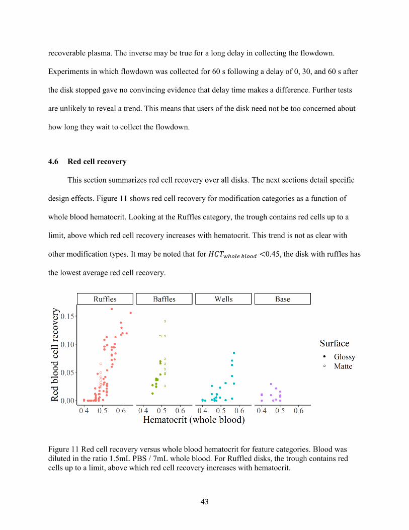
43

recoverable plasma. The inverse may be true for a long delay in collecting the flowdown.

Experiments in which flowdown was collected for 60 s following a delay of 0, 30, and 60 s after

the disk stopped gave no convincing evidence that delay time makes a difference. Further tests

are unlikely to reveal a trend. This means that users of the disk need not be too concerned about

how long they wait to collect the flowdown.

4.6 Red cell recovery

This section summarizes red cell recovery over all disks. The next sections detail specific

design effects. Figure 11 shows red cell recovery for modification categories as a function of

whole blood hematocrit. Looking at the Ruffles category, the trough contains red cells up to a

limit, above which red cell recovery increases with hematocrit. This trend is not as clear with

other modification types. It may be noted that for 𝐻𝐶𝑇𝑤ℎ𝑜𝑙𝑒 𝑏𝑙𝑜𝑜𝑑 <0.45, the disk with ruffles has

the lowest average red cell recovery.

Figure 11 Red cell recovery versus whole blood hematocrit for feature categories. Blood was

diluted in the ratio 1.5mL PBS / 7mL whole blood. For Ruffled disks, the trough contains red

cells up to a limit, above which red cell recovery increases with hematocrit.

44

4.6.1 Trough volume

The trough volume of 4 mL was designed to hold all red cells for 𝐻𝐶𝑇 ≤ 0.57 (4 mL/7 mL)

assuming the red cells are fully packed to 𝐻𝐶𝑇 = 1. Samples taken from the bottom of the

trough after a spin at 3000 RPM for 54 s gave 𝐻𝐶𝑇 = 0.855 (±0.015 95% confidence). Using

this value of 𝐻𝐶𝑇 in the cell pack, a 4 mL trough should accommodate 𝐻𝐶𝑇 > 0.486.

However, red cell flowdown still occurs despite predicted excess trough volume. As the

disk slows, the body force vector rotates smoothly downward and decreases from 600xg to 1xg

over ~2 minutes. The denser red cell sediment then is thought to slide from the outer wall down

into the trough. How do red cell recoveries change with trough depth? The trough depth was

varied (at the same width) to hold 3, 4 and 5 mL. Each disk was spun with 6, 7 and 8 mL of

whole blood/PBS at a same dilution ratio (1.5 mL/7 mL) to see if the trough depth quantitatively

changed red cell recovery. Figure 12 shows red cell recoveries from an overlaid linear model

[𝐻𝐶𝑇|𝑅𝑅 × 𝐷𝑖𝑠𝑘]. Red cell recovery stays at 0 until a threshold hematocrit, after which red cell

recovery increases linearly with hematocrit. The threshold hematocrits are predicted from the

regression intercepts. They increase from 0.449 (±0.014 95% confidence) at 3 mL to 0.492

(±0.025 95% conf) at 5 mL troughs. The x-intercept increases with hematocrit and at 5 mL

approaches the hypothetical threshold 0.486 calculated using the experimental trough packing

factor (0.855). The red cell recovery rate also decreases between 3 mL and 5 mL from 1.50

RBC/HCT (±0.25 95% confidence) to 0.94 RBC/HCT (±0.21 95% confidence). The lower red

cell recovery rate for 5 mL means that deeper troughs contain red cells better than shallow ones

do.

There is a transition region around 𝐻𝐶𝑇 = 0.46 for the 4 mL disk where red cell recovery

is not linear. This suggests a fuzzy interface between plasma and red cells after spindown. PEO

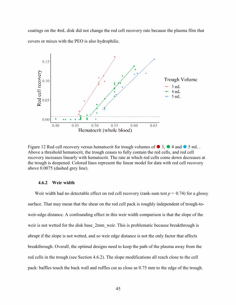
45

coatings on the 4mL disk did not change the red cell recovery rate because the plasma film that

covers or mixes with the PEO is also hydrophilic.

Figure 12 Red cell recovery versus hematocrit for trough volumes of 3, 4 and 5 mL .

Above a threshold hematocrit, the trough ceases to fully contain the red cells, and red cell

recovery increases linearly with hematocrit. The rate at which red cells come down decreases at

the trough is deepened. Colored lines represent the linear model for data with red cell recovery

above 0.0075 (dashed grey line).

4.6.2 Weir width

Weir width had no detectable effect on red cell recovery (rank-sum test p = 0.74) for a glossy

surface. That may mean that the shear on the red cell pack is roughly independent of trough-to-

weir-edge distance. A confounding effect in this weir width comparison is that the slope of the

weir is not wetted for the disk base_2mm_weir. This is problematic because breakthrough is

abrupt if the slope is not wetted, and so weir edge distance is not the only factor that affects

breakthrough. Overall, the optimal designs need to keep the path of the plasma away from the

red cells in the trough (see Section 4.6.2). The slope modifications all reach close to the cell

pack: baffles touch the back wall and ruffles cut as close as 0.75 mm to the edge of the trough.

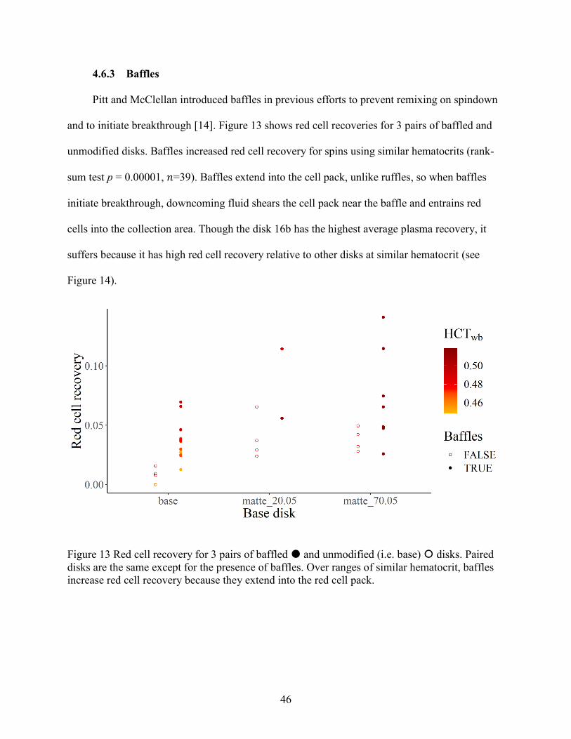
46

4.6.3 Baffles

Pitt and McClellan introduced baffles in previous efforts to prevent remixing on spindown

and to initiate breakthrough [14]. Figure 13 shows red cell recoveries for 3 pairs of baffled and

unmodified disks. Baffles increased red cell recovery for spins using similar hematocrits (rank-

sum test p = 0.00001, 𝑛=39). Baffles extend into the cell pack, unlike ruffles, so when baffles

initiate breakthrough, downcoming fluid shears the cell pack near the baffle and entrains red

cells into the collection area. Though the disk 16b has the highest average plasma recovery, it

suffers because it has high red cell recovery relative to other disks at similar hematocrit (see

Figure 14).

Figure 13 Red cell recovery for 3 pairs of baffled and unmodified (i.e. base) disks. Paired

disks are the same except for the presence of baffles. Over ranges of similar hematocrit, baffles

increase red cell recovery because they extend into the red cell pack.

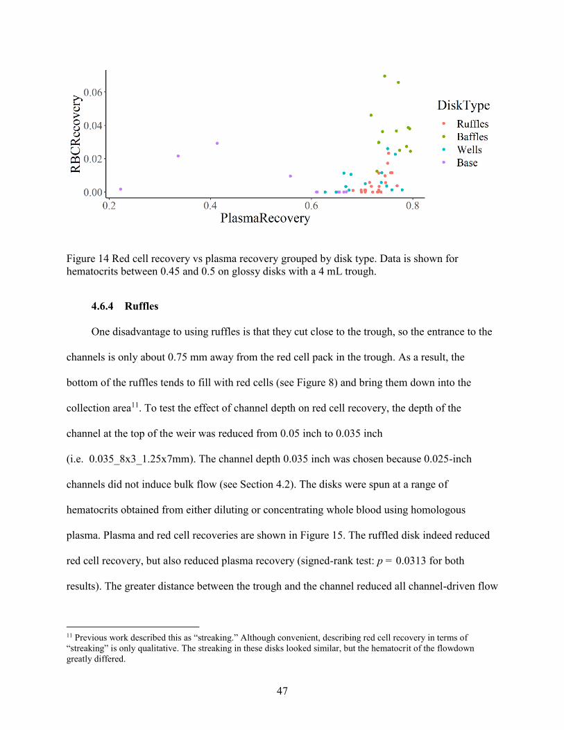
47

Figure 14 Red cell recovery vs plasma recovery grouped by disk type. Data is shown for

hematocrits between 0.45 and 0.5 on glossy disks with a 4 mL trough.

4.6.4 Ruffles

One disadvantage to using ruffles is that they cut close to the trough, so the entrance to the

channels is only about 0.75 mm away from the red cell pack in the trough. As a result, the

bottom of the ruffles tends to fill with red cells (see Figure 8) and bring them down into the

collection area11. To test the effect of channel depth on red cell recovery, the depth of the

channel at the top of the weir was reduced from 0.05 inch to 0.035 inch

(i.e. 0.035_8x3_1.25x7mm). The channel depth 0.035 inch was chosen because 0.025-inch

channels did not induce bulk flow (see Section 4.2). The disks were spun at a range of

hematocrits obtained from either diluting or concentrating whole blood using homologous

plasma. Plasma and red cell recoveries are shown in Figure 15. The ruffled disk indeed reduced

red cell recovery, but also reduced plasma recovery (signed-rank test: p = 0.0313 for both

results). The greater distance between the trough and the channel reduced all channel-driven flow

11 Previous work described this as “streaking.” Although convenient, describing red cell recovery in terms of

“streaking” is only qualitative. The streaking in these disks looked similar, but the hematocrit of the flowdown

greatly differed.

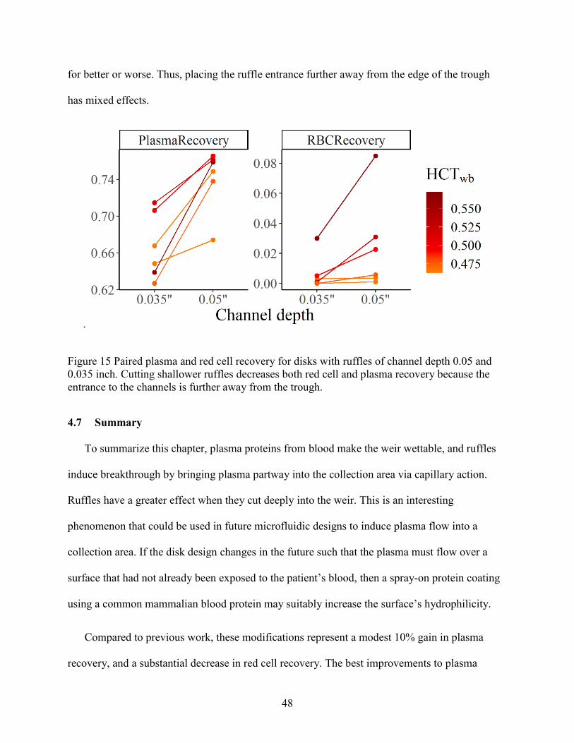
48

for better or worse. Thus, placing the ruffle entrance further away from the edge of the trough

has mixed effects.

.

Figure 15 Paired plasma and red cell recovery for disks with ruffles of channel depth 0.05 and

0.035 inch. Cutting shallower ruffles decreases both red cell and plasma recovery because the

entrance to the channels is further away from the trough.

4.7 Summary

To summarize this chapter, plasma proteins from blood make the weir wettable, and ruffles

induce breakthrough by bringing plasma partway into the collection area via capillary action.

Ruffles have a greater effect when they cut deeply into the weir. This is an interesting

phenomenon that could be used in future microfluidic designs to induce plasma flow into a

collection area. If the disk design changes in the future such that the plasma must flow over a

surface that had not already been exposed to the patient’s blood, then a spray-on protein coating

using a common mammalian blood protein may suitably increase the surface’s hydrophilicity.

Compared to previous work, these modifications represent a modest 10% gain in plasma

recovery, and a substantial decrease in red cell recovery. The best improvements to plasma

49

recovery were made by a combination of ruffles and wells on a glossy surface. Baffles also

induced even breakthrough but entrained more red cells. Modifications that extended close to the

trough increased red cell recovery. Future work should try to recover the meniscus fluid using

perhaps a downward-sloped weir top and wells only.

50

5 MODELED AND EXPERIMENTAL EFFECTS OF BLOOD DILUTION

The purpose of modeling sedimentation is to predict how the dilution of blood will change

red cell and bacteria separation without having to do experiments for each proposed condition.

Predicting red cell and bacteria separation purely from sensitive statistical models requires

prohibitively many experiments because experimental variability is high. Instead, this section

uses a numerical model to explore how red cell sedimentation changes with hematocrit. It aims

to find the shortest spin time possible to remove all red cells from suspension. It does not model

bacteria sedimentation, but insight from the model informs us of spin times and dilution amounts

to use in carefully designed experiments in an effort to minimize red cell recovery and maximize

bacteria recovery.

5.1 Sedimentation time

Previous work reduced the variables of spin time and spin speed to a single experimental

variable by defining a metric called characteristic length [14]. The characteristic length is the

distance that an 8-µm sphere with the same physical properties as an RBC (see Table 2 in

Appendix A) would travel in a given time period when exposed to a time-varying centrifugal

field. It is the time integral of Stokes velocity. Pitt et al. showed that both red cell and bacteria

recovery decrease with characteristic length [14]. However, this characteristic length did not

consider RBC shape, hindered settling, or the cell pack thickness.

51

The current model addresses these shortcomings but reduces dimensionality differently.

The spatial and time domains are non-dimensionalized using parameters introduced by Lerche’s

method [36], namely:

𝑟∗ =

𝑟 − 𝑅𝑎𝑖𝑟

𝑅𝑤𝑎𝑙𝑙 − 𝑅𝑎𝑖𝑟=

𝑟 − 𝑅𝑎𝑖𝑟

𝐿, 5-1

𝑇 =

𝐿

𝑢𝑅𝐵𝐶,∞

, 5-2

𝑡∗ =

𝑡

𝑇=

𝑡𝑢𝑅𝐵𝐶,∞

𝐿. 5-3

Here, 𝑟 is the spatial coordinate measured radially outward from the air-blood interface that

exists when the disk is spinning at 𝑅𝑎𝑖𝑟 = 56.7 mm until the outer disk wall at 𝑅𝑤𝑎𝑙𝑙 = 60 mm. 𝐿

is the nominal thickness of the fluid in the radial direction (𝐿 = 3.3 mm in the experiments of

this chapter), and 𝑢𝑅𝐵𝐶,∞ = 0.638 mm/s is the Stokes velocity for red blood cells calculated

using Lerche’s physical parameters (See Table 2 in Appendix A) evaluated at 𝑅𝑤𝑎𝑙𝑙 and at 3000

RPM. The dimensionless radial coordinate 𝑟∗ ∈ [0,1] extends outward from the inner edge of the

fluid to the disk wall. The time constant 𝑇 = 4.7 s is how long a single RBC at infinite dilution

would take to traverse the entire spatial domain of diluted blood, and thus 𝑡∗ is the number of

elapsed travel times at infinite dilution.12

The current spin profile requires 2 minutes to decelerate from 3000 RPM in order to

prevent remixing between the cell pack and the plasma, during which the Stokes velocity

changes. Both the characteristic length and the conservation law models, however, assume a

constant Stokes velocity. For a spin profile comprised of spin up to 3000 RPM, 0 s hold time,

12 The conversion between 𝐿𝑐ℎ𝑎𝑟 and 𝑡∗ is 𝑡∗ = 𝐿𝑐ℎ𝑎𝑟/𝐿. This uses the identity 𝐿𝑐ℎ𝑎𝑟 = ∫ 𝑢𝑅𝐵𝐶,∞

(𝑡)𝑑𝑡𝑡𝑒𝑛𝑑

0=

𝑢𝑅𝐵𝐶,∞𝑡, where 𝑢𝑅𝐵𝐶,∞ is the time-averaged Stokes velocity.

52

and spin down, integrating the dynamic angular velocity profile divided by the maximum angular

velocity gives the integral ∫ω(𝑡)2

ω𝑚𝑎𝑥2 𝑑𝑡

𝑡𝑒𝑛𝑑

0= 0.055. This shows that ignoring the transient parts of

the spin profile only introduces a 5.5% error to the time-averaged Stokes velocity. Thus,

estimates from any model that uses a constant Stokes velocity will underpredict dimensionless

quantities by at most 5.5% at a hold time of 0 s. This error shrinks with increasing hold time.

Furthermore, 𝐿 only changes by about ±2% with pipetting error of ±0.1 mL (an extreme error).

The continuity equation described in Section 2.4 (Equation 2-10) is non-dimensionalized

to Equation 5-5:

1

𝑇

𝜕𝜙

𝜕𝑡∗+

𝑢𝑅𝐵𝐶,∞

𝐿

𝜕𝑓(𝜙)

𝜕𝑟∗= 0, 5-4

𝜕𝜙

𝜕𝑡∗+

𝜕𝑓(𝜙)

𝜕𝑟∗= 0, 5-5

where 𝑓(𝜙) = 𝜙𝑣(𝜙) = 𝜙(1 − 𝜙)ℎ𝑠𝑐(𝜙) is a dimensionless red cell volume flux determined

from the hindered settling function ℎ𝑠𝑐(𝜙). Modeling a cylindrical system with cartesian

coordinates is generally inappropriate. However, the ratio 𝑅𝑎𝑖𝑟/𝑅𝑤𝑎𝑙𝑙 for the annulus-shaped

fluid ring is 0.945 (5.67 cm/6 cm, see Table 5 in Appendix A), so the error is on the order of 5%.

Furthermore, Detloff showed experimentally and numerically that the suspension-clear fluid

(SC) interface moved at the same rate for cylindrical and cartesian geometries [49].

Numerically integrating Equation 5-5 using Godunov’s flux function (Equation 2-17)

with boundary conditions 𝜙 = 0 at 𝑟∗ = 0 and 𝜙 = 𝜙𝑚𝑎𝑥 = 0.97 at 𝑟∗ = 1 gives sedimentation

profiles such as in Figure 16. Detailed code is available in Section A.6. Each plot in Figure 16

shows iso-hematocrit lines in dimensionless space and time. In each graph, the downward-sloped

line crossing through 𝑟∗ = 0 is the red cell suspension-clear fluid (SC) interface, and the upward-

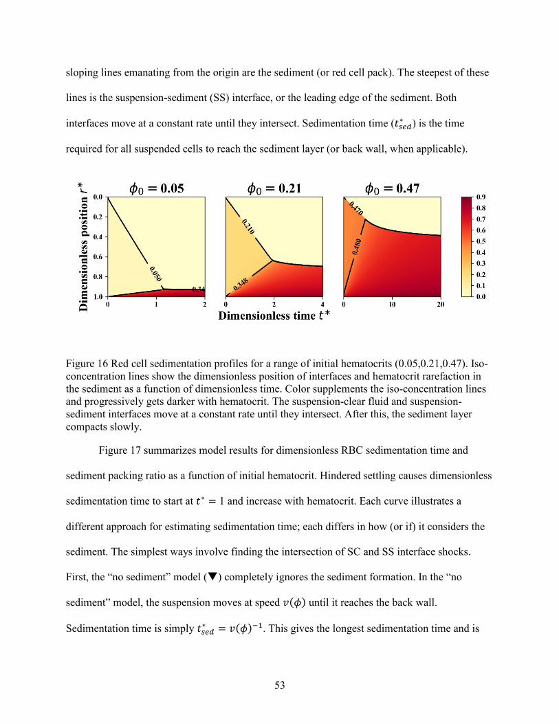
53

sloping lines emanating from the origin are the sediment (or red cell pack). The steepest of these

lines is the suspension-sediment (SS) interface, or the leading edge of the sediment. Both

interfaces move at a constant rate until they intersect. Sedimentation time (𝑡𝑠𝑒𝑑∗ ) is the time

required for all suspended cells to reach the sediment layer (or back wall, when applicable).

Figure 16 Red cell sedimentation profiles for a range of initial hematocrits (0.05,0.21,0.47). Iso-

concentration lines show the dimensionless position of interfaces and hematocrit rarefaction in

the sediment as a function of dimensionless time. Color supplements the iso-concentration lines

and progressively gets darker with hematocrit. The suspension-clear fluid and suspension-

sediment interfaces move at a constant rate until they intersect. After this, the sediment layer

compacts slowly.

Figure 17 summarizes model results for dimensionless RBC sedimentation time and

sediment packing ratio as a function of initial hematocrit. Hindered settling causes dimensionless

sedimentation time to start at 𝑡∗ = 1 and increase with hematocrit. Each curve illustrates a

different approach for estimating sedimentation time; each differs in how (or if) it considers the

sediment. The simplest ways involve finding the intersection of SC and SS interface shocks.

First, the “no sediment” model () completely ignores the sediment formation. In the “no

sediment” model, the suspension moves at speed 𝑣(𝜙) until it reaches the back wall.

Sedimentation time is simply 𝑡𝑠𝑒𝑑∗ = 𝑣(𝜙)−1. This gives the longest sedimentation time and is

54

the least realistic. Second, the “instant compaction” model () assumes that sediment does form,

but that it compacts immediately to 𝜙 = 𝜙𝑚𝑎𝑥. Here, 𝑡𝑠𝑒𝑑∗ is the intersection in the 𝑟∗-𝑡∗ plane

between the SC interface13

𝑟𝑆𝐶∗ = 𝑣(𝜙0)𝑡∗ 5-6

and the SS interface

𝑟𝑆𝑆

∗ = 1 −𝑓(𝜙0) − 𝑓(𝜙𝑚𝑎𝑥)

𝜙0 − 𝜙𝑚𝑎𝑥𝑡∗ = 1 −

𝑓(𝜙0)

𝜙0 − 𝜙𝑚𝑎𝑥𝑡∗ 5-7

to give the final expression

𝑡𝑠𝑒𝑑

∗ = (𝑣(𝜙0) +𝜙0𝑣(𝜙0)

𝜙𝑚𝑎𝑥 − 𝜙0)

−1

. 5-8

Here, rarefaction is ignored, and the SC and SS interfaces move toward each other with fixed

(but different) velocity; they intersect before the suspension reaches the back wall, reducing 𝑡𝑠𝑒𝑑∗

below that of the “no sediment” model. The “instant compaction” model is more realistic, but it

does not account well for the slow compaction of red cell sediment predicted by the hindered

settling corrections14.

The third “rarefaction” model includes the sediment and allows it to compact according

to the flux curve. The “rarefaction” model is identical to the “instant compaction” model, except

that the SS interface moves at a speed given by 𝑓′(𝜙𝑟𝑎𝑟𝑒), where 𝜙𝑟𝑎𝑟𝑒 is the hematocrit on the

sediment side of the SS interface15. Although this method should be the most realistic, it gives

unphysical solutions at low hematocrit in which the sediment compacts to 𝜙 > 𝜙𝑚𝑎𝑥; the reason

13 The 𝑟∗ limits in Figure 17 makes these equations seem backward, but the equations are correct. 14 This model violates the entropy condition because the shock connecting 𝑓(𝜙0) to 𝑓(𝜙𝑚𝑎𝑥) crosses the flux curve,

but it may be a useful approximation anyway because the flux curve is an empirical function. 15 𝜙𝑟𝑎𝑟𝑒 is the point of tangency on the flux curve connecting 𝜙0 to 𝜙𝑚𝑎𝑥 obtained from the stretched string analogy.

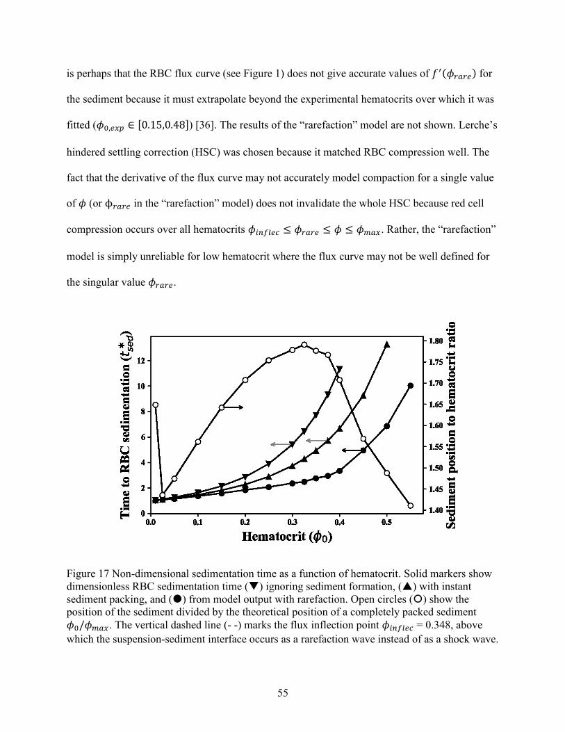
55

is perhaps that the RBC flux curve (see Figure 1) does not give accurate values of 𝑓′(𝜙𝑟𝑎𝑟𝑒) for

the sediment because it must extrapolate beyond the experimental hematocrits over which it was

fitted (𝜙0,𝑒𝑥𝑝 ∈ [0.15,0.48]) [36]. The results of the “rarefaction” model are not shown. Lerche’s

hindered settling correction (HSC) was chosen because it matched RBC compression well. The

fact that the derivative of the flux curve may not accurately model compaction for a single value

of 𝜙 (or ϕ𝑟𝑎𝑟𝑒 in the “rarefaction” model) does not invalidate the whole HSC because red cell

compression occurs over all hematocrits 𝜙𝑖𝑛𝑓𝑙𝑒𝑐 ≤ 𝜙𝑟𝑎𝑟𝑒 ≤ 𝜙 ≤ 𝜙𝑚𝑎𝑥. Rather, the “rarefaction”

model is simply unreliable for low hematocrit where the flux curve may not be well defined for

the singular value 𝜙𝑟𝑎𝑟𝑒.

Figure 17 Non-dimensional sedimentation time as a function of hematocrit. Solid markers show

dimensionless RBC sedimentation time () ignoring sediment formation, () with instant

sediment packing, and () from model output with rarefaction. Open circles () show the

position of the sediment divided by the theoretical position of a completely packed sediment

𝜙0/𝜙𝑚𝑎𝑥. The vertical dashed line (- -) marks the flux inflection point 𝜙𝑖𝑛𝑓𝑙𝑒𝑐 = 0.348, above

which the suspension-sediment interface occurs as a rarefaction wave instead of as a shock wave.

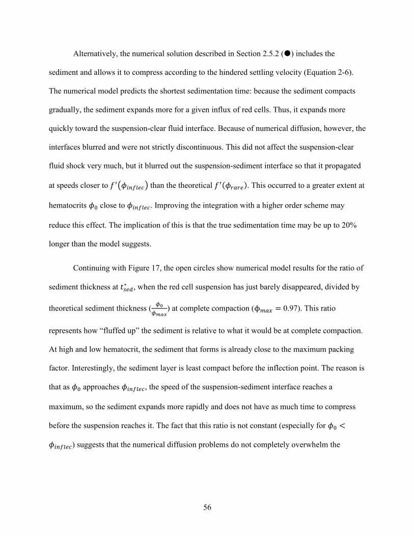
56

Alternatively, the numerical solution described in Section 2.5.2 () includes the

sediment and allows it to compress according to the hindered settling velocity (Equation 2-6).

The numerical model predicts the shortest sedimentation time: because the sediment compacts

gradually, the sediment expands more for a given influx of red cells. Thus, it expands more

quickly toward the suspension-clear fluid interface. Because of numerical diffusion, however, the

interfaces blurred and were not strictly discontinuous. This did not affect the suspension-clear

fluid shock very much, but it blurred out the suspension-sediment interface so that it propagated

at speeds closer to 𝑓′(𝜙𝑖𝑛𝑓𝑙𝑒𝑐) than the theoretical 𝑓′(𝜙𝑟𝑎𝑟𝑒). This occurred to a greater extent at

hematocrits 𝜙0 close to 𝜙𝑖𝑛𝑓𝑙𝑒𝑐. Improving the integration with a higher order scheme may

reduce this effect. The implication of this is that the true sedimentation time may be up to 20%

longer than the model suggests.

Continuing with Figure 17, the open circles show numerical model results for the ratio of

sediment thickness at 𝑡𝑠𝑒𝑑∗ , when the red cell suspension has just barely disappeared, divided by

theoretical sediment thickness (𝜙0

𝜙𝑚𝑎𝑥) at complete compaction (ϕ𝑚𝑎𝑥 = 0.97). This ratio

represents how “fluffed up” the sediment is relative to what it would be at complete compaction.

At high and low hematocrit, the sediment that forms is already close to the maximum packing

factor. Interestingly, the sediment layer is least compact before the inflection point. The reason is

that as 𝜙0 approaches 𝜙𝑖𝑛𝑓𝑙𝑒𝑐, the speed of the suspension-sediment interface reaches a

maximum, so the sediment expands more rapidly and does not have as much time to compress

before the suspension reaches it. The fact that this ratio is not constant (especially for 𝜙0 <

𝜙𝑖𝑛𝑓𝑙𝑒𝑐) suggests that the numerical diffusion problems do not completely overwhelm the

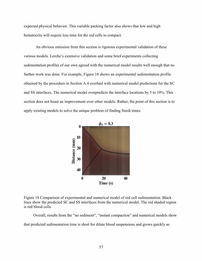
57

expected physical behavior. This variable packing factor also shows that low and high

hematocrits will require less time for the red cells to compact.

An obvious omission from this section is rigorous experimental validation of these

various models. Lerche’s extensive validation and some brief experiments collecting

sedimentation profiles of our own agreed with the numerical model results well enough that no

further work was done. For example, Figure 18 shows an experimental sedimentation profile

obtained by the procedure in Section A.4 overlaid with numerical model predictions for the SC

and SS interfaces. The numerical model overpredicts the interface locations by 5 to 10%. This

section does not boast an improvement over other models. Rather, the point of this section is to

apply existing models to solve the unique problem of finding finish times.

Figure 18 Comparison of experimental and numerical model of red cell sedimentation. Black

lines show the predicted SC and SS interfaces from the numerical model. The red shaded region

is red blood cells.

Overall, results from the “no sediment”, “instant compaction” and numerical models show

that predicted sedimentation time is short for dilute blood suspensions and grows quickly as

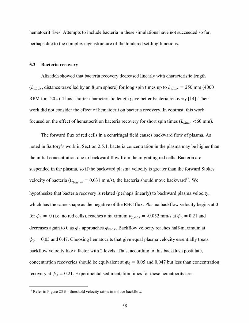
58

hematocrit rises. Attempts to include bacteria in these simulations have not succeeded so far,

perhaps due to the complex eigenstructure of the hindered settling functions.

5.2 Bacteria recovery

Alizadeh showed that bacteria recovery decreased linearly with characteristic length

(𝐿𝑐ℎ𝑎𝑟, distance travelled by an 8 µm sphere) for long spin times up to 𝐿𝑐ℎ𝑎𝑟 = 250 mm (4000

RPM for 120 s). Thus, shorter characteristic length gave better bacteria recovery [14]. Their

work did not consider the effect of hematocrit on bacteria recovery. In contrast, this work

focused on the effect of hematocrit on bacteria recovery for short spin times (𝐿𝑐ℎ𝑎𝑟 <60 mm).

The forward flux of red cells in a centrifugal field causes backward flow of plasma. As

noted in Sartory’s work in Section 2.5.1, bacteria concentration in the plasma may be higher than

the initial concentration due to backward flow from the migrating red cells. Bacteria are

suspended in the plasma, so if the backward plasma velocity is greater than the forward Stokes

velocity of bacteria (𝑢𝑏𝑎𝑐,∞ = 0.031 mm/s), the bacteria should move backward16. We

hypothesize that bacteria recovery is related (perhaps linearly) to backward plasma velocity,

which has the same shape as the negative of the RBC flux. Plasma backflow velocity begins at 0

for 𝜙0 = 0 (i.e. no red cells), reaches a maximum 𝑣𝑝,𝑎𝑏𝑠 = -0.052 mm/s at 𝜙0 = 0.21 and

decreases again to 0 as 𝜙0 approaches 𝜙𝑚𝑎𝑥. Backflow velocity reaches half-maximum at

𝜙0 = 0.05 and 0.47. Choosing hematocrits that give equal plasma velocity essentially treats

backflow velocity like a factor with 2 levels. Thus, according to this backflush postulate,

concentration recoveries should be equivalent at 𝜙0 = 0.05 and 0.047 but less than concentration

recovery at 𝜙0 = 0.21. Experimental sedimentation times for these hematocrits are

16 Refer to Figure 23 for threshold velocity ratios to induce backflow.

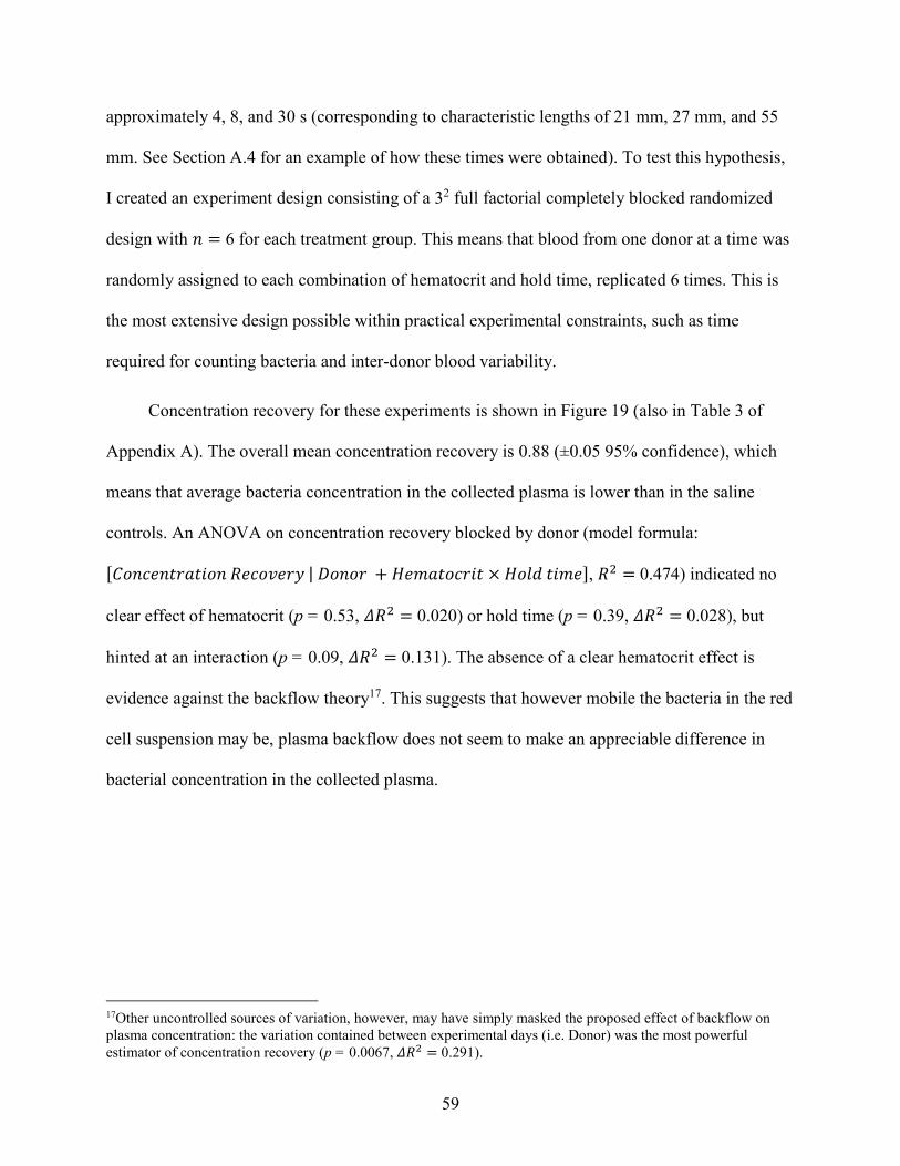
59

approximately 4, 8, and 30 s (corresponding to characteristic lengths of 21 mm, 27 mm, and 55

mm. See Section A.4 for an example of how these times were obtained). To test this hypothesis,

I created an experiment design consisting of a 32 full factorial completely blocked randomized

design with 𝑛 = 6 for each treatment group. This means that blood from one donor at a time was

randomly assigned to each combination of hematocrit and hold time, replicated 6 times. This is

the most extensive design possible within practical experimental constraints, such as time

required for counting bacteria and inter-donor blood variability.

Concentration recovery for these experiments is shown in Figure 19 (also in Table 3 of

Appendix A). The overall mean concentration recovery is 0.88 (±0.05 95% confidence), which

means that average bacteria concentration in the collected plasma is lower than in the saline

controls. An ANOVA on concentration recovery blocked by donor (model formula:

[𝐶𝑜𝑛𝑐𝑒𝑛𝑡𝑟𝑎𝑡𝑖𝑜𝑛 𝑅𝑒𝑐𝑜𝑣𝑒𝑟𝑦 | 𝐷𝑜𝑛𝑜𝑟  + 𝐻𝑒𝑚𝑎𝑡𝑜𝑐𝑟𝑖𝑡 × 𝐻𝑜𝑙𝑑 𝑡𝑖𝑚𝑒], 𝑅2 = 0.474) indicated no

clear effect of hematocrit (p = 0.53, 𝛥𝑅2 = 0.020) or hold time (p = 0.39, 𝛥𝑅2 = 0.028), but

hinted at an interaction (p = 0.09, 𝛥𝑅2 = 0.131). The absence of a clear hematocrit effect is

evidence against the backflow theory17. This suggests that however mobile the bacteria in the red

cell suspension may be, plasma backflow does not seem to make an appreciable difference in

bacterial concentration in the collected plasma.

17Other uncontrolled sources of variation, however, may have simply masked the proposed effect of backflow on

plasma concentration: the variation contained between experimental days (i.e. Donor) was the most powerful

estimator of concentration recovery (p = 0.0067, 𝛥𝑅2 = 0.291).

60

Figure 19 Concentration recovery as a function of hematocrit (𝐻𝐶𝑇𝑑𝑖𝑙𝑢𝑡𝑒𝑑 = 0.05, 0.21, and

0.47) for hold times 4, 8, and 30 s. Concentration recovery does not appreciably change. 95%

confidence interval shown for each group. Offset in the x-axis is for ease of display. 4 outlier

replicates and 1 failed experiment are omitted from this figure and from Figure 19.

Figure 20 Bacteria recovery as a function of hematocrit (𝐻𝐶𝑇𝑑𝑖𝑙𝑢𝑡𝑒𝑑 = 0.05, 0.21, and 0.47) for

hold times 4, 8, and 30 s. Bacteria recovery decreases linearly with 𝐻𝐶𝑇𝑑𝑖𝑙𝑢𝑡𝑒𝑑 (𝛽0 = 0.68,

𝛽1 = -0.63). 95% confidence interval shown for each group and for regression model. Offset in

the x-axis is for ease of display.

61

Bacterial concentration is only one part of bacteria recovery: the total recovered volume

also defines overall bacteria recovery. To correctly model overall bacteria recovery in our disk,

we must integrate the bacteria concentration all the way from the air-plasma interface at 𝑟∗ = 0

to a threshold 𝑟𝑓𝑙𝑜𝑤𝑑𝑜𝑤𝑛∗ on the spatial axis above which everything flows down. The location of

that interface in dimensionless space can be obtained by simply dividing volumetric flowdown

by the total input volume to get the total volumetric recovery18:

𝑉𝑜𝑙𝑢𝑚𝑒 𝑟𝑒𝑐𝑜𝑣𝑒𝑟𝑦 = 𝑟𝑓𝑙𝑜𝑤𝑑𝑜𝑤𝑛

∗ =𝑉𝑓𝑙𝑜𝑤𝑑𝑜𝑤𝑛

𝑉𝑤ℎ𝑜𝑙𝑒 𝑏𝑙𝑜𝑜𝑑 + 𝑉𝑃𝐵𝑆. 5-9

In this study, the trough volumes were designed to hold all the red cells for each

hematocrit, correlating volume recovery very closely with (1 − 𝐻𝐶𝑇𝑑𝑖𝑙𝑢𝑡𝑒𝑑). Instead of volume

recovery, however, we will use (1 − 𝐻𝐶𝑇𝑑𝑖𝑙𝑢𝑡𝑒𝑑). Of the total suspension volume, only the

fraction (1 − 𝐻𝐶𝑇𝑑𝑖𝑙𝑢𝑡𝑒𝑑) is collectable; so, without any enrichment of bacteria in the flowdown,

bacteria recovery should decrease linearly with hematocrit. Figure 20 shows bacteria recovery as

a function of 𝐻𝐶𝑇𝑑𝑖𝑙𝑢𝑡𝑒𝑑. A linear model [𝐵𝑎𝑐𝑡𝑒𝑟𝑖𝑎 𝑟𝑒𝑐𝑜𝑣𝑒𝑟𝑦 | 𝐷𝑜𝑛𝑜𝑟 + 𝐻𝑒𝑚𝑎𝑡𝑜𝑐𝑟𝑖𝑡] gives a

slope β1 = -0.633 BR/HCT (±0.163 95% confidence, 𝛥𝑅2 = 0.44) and intercept β0 = 0.681

(±0.05 95% confidence). Bacteria recovery is directly proportional to the fraction of recoverable

fluid. This makes sense physically. What is surprising is that it occurs not in a 1:1 ratio. That is,

dilution does not recover bacteria at as great a rate as expected. Indeed, this model predicts

approximately 0 bacteria recovery at 𝐻𝐶𝑇𝑑𝑖𝑙𝑢𝑡𝑒𝑑 = 1, which supports the theory that bacteria

recovery is proportional to recoverable fluid volume. But the fact that only 70% of the bacteria

18 Defining Volume Recovery in terms of “recoverable fluid” (i.e. the total input volume minus the trough volume)

may be more suitable if disks are designed to hold a fixed amount of red cells, as in these experiments. Defined this

way, the fraction 0.84 (±0.01 95% confidence) of the recoverable fluid was collected in these experiments, and

𝑟𝑓𝑙𝑜𝑤𝑑𝑜𝑤𝑛∗ = 0.84(1 − 𝐻𝐶𝑇𝑑𝑖𝑙𝑢𝑡𝑒𝑑/0.85)

62

are recovered at 𝐻𝐶𝑇 = 0 is puzzling19. At 𝐻𝐶𝑇 = 0.05, fluid holdup from the trough and the

residual meniscus around the weir only account for 20% of the total fluid. That means that on

average, an extra 10% of the bacteria is unaccounted for. Whereas the exact cause of this

inefficiency is unknown, the overall bacterial response clearly decreases with hematocrit. This

suffices to answer the question of how much to dilute the blood, which is the topic of the next

section.

5.3 Dilution optimization

When deciding how much to dilute the blood, there are several competing objectives.

Diluting the blood leads to better bacterial recovery but can also drastically increase the amount

of processed fluid. This section breaks down the question of dilution into a mathematical

optimization problem. Downstream antibiotic susceptibility testing will likely concentrate the

bacteria suspension via filtering or further centrifugation before processing it, so we care about

the raw number of bacteria (𝑁𝑏𝑎𝑐,𝑓𝑑) that are recovered more than the concentration at which we

recover them. An expression for 𝑁𝑏𝑎𝑐,𝑓𝑑 normalized by starting concentration 𝐶𝑏𝑎𝑐,𝑤𝑏 is:

𝑁𝑏𝑎𝑐,𝑓𝑑

𝐶𝑏𝑎𝑐,𝑤𝑏= 𝑉𝑤𝑏𝑓(𝐻𝐶𝑇𝑑𝑖𝑙𝑢𝑡𝑒𝑑, 𝑡),

5-10

where 𝑓 = 𝛽0 + 𝛽1𝐻𝐶𝑇𝑑𝑖𝑙𝑢𝑡𝑒𝑑 predicts bacterial recovery as a function of initial hematocrit

(𝐻𝐶𝑇𝑑𝑖𝑙𝑢𝑡𝑒𝑑) and hold time (𝑡) from the bacteria recovery experiments. Here, 𝑁𝑏𝑎𝑐,𝑓𝑑 increases

linearly with 𝑉𝑤𝑏 and decreases linearly with 𝐻𝐶𝑇𝑑𝑖𝑙𝑢𝑡𝑒𝑑. So, 𝑁𝑏𝑎𝑐,𝑓𝑑 reaches a maximum at

19 It is true that both of these intercepts extrapolate the data. For reference, fractional bacteria recovery in pure saline

is also a surprisingly low 0.61 (±0.10 95% confidence) for a hold time of 4 seconds on the disk designed for

𝐻𝐶𝑇 = 0.05. Extrapolating to 𝐻𝐶𝑇 = 1.0 has no support at this time.

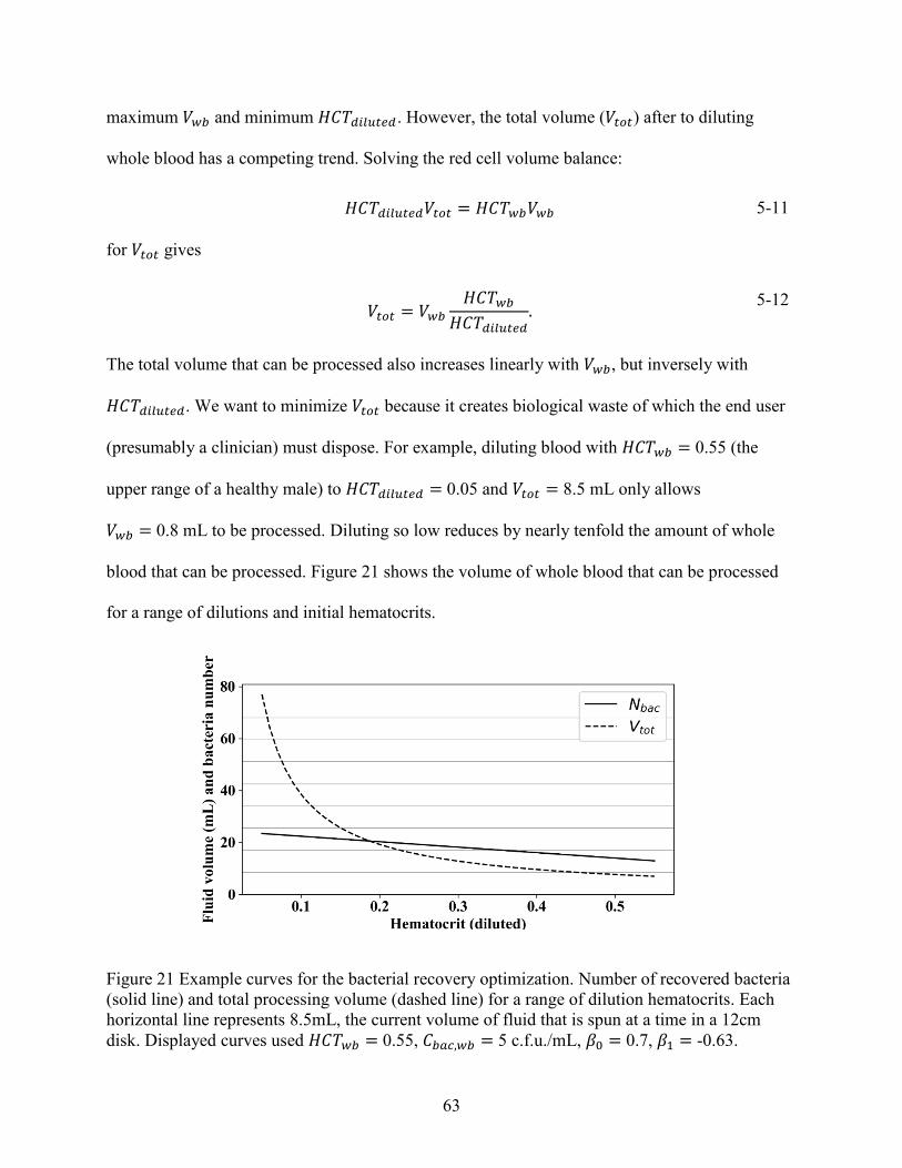
63

maximum 𝑉𝑤𝑏 and minimum 𝐻𝐶𝑇𝑑𝑖𝑙𝑢𝑡𝑒𝑑. However, the total volume (𝑉𝑡𝑜𝑡) after to diluting

whole blood has a competing trend. Solving the red cell volume balance:

𝐻𝐶𝑇𝑑𝑖𝑙𝑢𝑡𝑒𝑑𝑉𝑡𝑜𝑡 = 𝐻𝐶𝑇𝑤𝑏𝑉𝑤𝑏 5-11

for 𝑉𝑡𝑜𝑡 gives

𝑉𝑡𝑜𝑡 = 𝑉𝑤𝑏

𝐻𝐶𝑇𝑤𝑏

𝐻𝐶𝑇𝑑𝑖𝑙𝑢𝑡𝑒𝑑.

5-12

The total volume that can be processed also increases linearly with 𝑉𝑤𝑏, but inversely with

𝐻𝐶𝑇𝑑𝑖𝑙𝑢𝑡𝑒𝑑. We want to minimize 𝑉𝑡𝑜𝑡 because it creates biological waste of which the end user

(presumably a clinician) must dispose. For example, diluting blood with 𝐻𝐶𝑇𝑤𝑏 = 0.55 (the

upper range of a healthy male) to 𝐻𝐶𝑇𝑑𝑖𝑙𝑢𝑡𝑒𝑑 = 0.05 and 𝑉𝑡𝑜𝑡 = 8.5 mL only allows

𝑉𝑤𝑏 = 0.8 mL to be processed. Diluting so low reduces by nearly tenfold the amount of whole

blood that can be processed. Figure 21 shows the volume of whole blood that can be processed

for a range of dilutions and initial hematocrits.

Figure 21 Example curves for the bacterial recovery optimization. Number of recovered bacteria

(solid line) and total processing volume (dashed line) for a range of dilution hematocrits. Each

horizontal line represents 8.5mL, the current volume of fluid that is spun at a time in a 12cm

disk. Displayed curves used 𝐻𝐶𝑇𝑤𝑏 = 0.55, 𝐶𝑏𝑎𝑐,𝑤𝑏 = 5 c.f.u./mL, 𝛽0 = 0.7, 𝛽1 = -0.63.

64

Summing Equations 5-10 and 5-12 with the positive-valued weights 𝑤𝑏𝑎𝑐 and 𝑤𝑑𝑖𝑙 gives

the objective function

𝑚𝑖𝑛

𝑠.𝑡. 𝐻𝐶𝑇𝑑𝑖𝑙𝑢𝑡𝑒𝑑>0𝑉𝑤𝑏 [𝑤𝑏𝑎𝑐(𝛽0 + 𝛽1𝐻𝐶𝑇𝑑𝑖𝑙𝑢𝑡𝑒𝑑) + 𝑤𝑑𝑖𝑙

𝐻𝐶𝑇𝑤𝑏

𝐻𝐶𝑇𝑑𝑖𝑙𝑢𝑡𝑒𝑑], 5-13

where 𝑤𝑏𝑎𝑐 ($/mL whole blood) is the perceived value of each bacterium and 𝑤𝑑𝑖𝑙 ($/mL

biofluid waste) is the cost of disposing of biohazard waste. Choice of weights will be motivated

by the disposal costs of processed plasma-saline solution and the benefit of recovering bacteria.

The optimal dilution hematocrit is given by:

HC𝑇𝑑𝑖𝑙𝑢𝑡𝑒𝑑,𝑜𝑝𝑡𝑖𝑚𝑎𝑙 = √wdilHCTwb

𝑤𝑏𝑎𝑐|β1| 5-14

A square-root dependence on 𝐻𝐶𝑇𝑤𝑏 in the objective function means that a lower volume of

whole blood can be processed for patients with high hematocrit (such as males) for a given

𝐻𝐶𝑇𝑑𝑖𝑙𝑢𝑡𝑒𝑑. This objective function only considers operating costs. Capital costs will increase

with dilution as the disks and the associated apparatus become larger and require more space in a

clinic.

5.4 Summary

The mathematical modeling presented in this chapter shows that dimensionless spin time

required to remove all red cells increases with hematocrit as the suspension moves more slowly.

Dimensionless sedimentation time can be easily scaled to dimensional time using fluid volume.

Experiments with blood dilution show that bacteria recovery scales linearly with the fraction of

recoverable volume for the short spin times described here.

65

6 CONCLUSIONS AND RECOMMENDATIONS

The overall purpose of this thesis was to facilitate antibiotic susceptibility tests by rapidly

separating bacteria from whole blood components which interfere with subsequent diagnostic

tests. The separation process quickly removes red blood cells from a sample, leaving behind

bacteria still suspended in the plasma, which is collected in preparation for antibiotic

susceptibility tests. It uses a hollow centrifugal disk to leverage hydrodynamic differences

between bacteria and blood components.

The specific aims of this work were to (1) maximize the fractional recovery of plasma and

minimize the fractional recovery of red cells by modifying the disk, (2) explore how diluting the

blood prior to spinning it might improve fractional bacteria recovery, and (3) mathematically

model the separation process. This section describes the progress made toward each goal and

recommends future work.

6.1 Conclusions

6.1.1 Aim 1: disk designs

There are several major findings regarding disk design that should inform future work.

First, a smooth disk surface greatly reduced variability in fractional plasma recovery. Dried

plasma coatings on a smooth surface made that surface very wettable by plasma, which

66

encouraged plasma to flow into an area where it can be collected. Although plasma coatings also

made rough surfaces more hydrophilic, the effect was not as pronounced.

Second, v-shaped channels that cut into the weir slope induced spontaneous capillary

flow of plasma, which improved fractional plasma recovery relative to the base design. These

channels, however, also pulled red cells into the collection area, which reduced the overall

separation efficiency. These two effects from the channels grew more pronounced with

increasing channel depth. Overall, three parallel v-shaped channels of half angle 20° are a helpful

addition in directing plasma flow.

Third, wells, or depressions in the collection area, did direct plasma flow into specific

locations for collection. The disk with 8 wells and ruffles (20.05_8x3_1.25x7mm) performed the

best.

Fourth, baffled disks recovered comparable amounts of plasma to disks with ruffles, but

they also entrained more red cells at similar hematocrits. Future designs should exclude baffles.

6.1.2 Aim 2: blood dilution and bacteria recovery

This work characterized the effect of blood dilution on bacteria recovery and suggested an

optimal dilution hematocrit as a function of costs and donor hematocrit. There are several major

conclusions.

First, because of the natural variation in these experiments, we could not measure the effect

of backflow on bacterial concentration. We believe on physical grounds that backflow does exist,

but that its effect was not detectable given other uncontrolled experimental variables.

67

Second, the optimal hematocrit to which blood should be diluted scales with the square root

of the donor’s whole blood hematocrit. The ultimate choice of dilution will depend on clinician

operating and disposal costs.

Third, the flow of diluted blood is easier to direct, and the blood contains enough proteins

to create a plasma-wettable film on the 3D printed material.

6.1.3 Aim 3: numerical model of sedimentation

Bacteria are separated from blood cells by removing the latter from suspension, and the

time it takes to remove all suspended red blood cells is called sedimentation time. Several

mathematical models for sedimentation time were explored, and their outcomes are described

here.

First, in all four models (“no sediment”, “instant compaction”, “rarefaction” and the

numerical model), sedimentation time started out short and increased with hematocrit.

Differences between model predictions grew with different starting hematocrit. Dimensionless

sedimentation time can be used to relate total processing volume with required spin time.

Second, the numerical model gives the most realistic estimates for sedimentation time

because it gives full detail for sediment compaction over time. For dilute blood, red cells

sediment much faster than bacteria, so the disk should only spin until all the red cells are gone,

since longer times will also reduce bacterial recovery.

Third, we adopted a Riemann-solver approach to model sedimentation in multicomponent

mixtures. This worked well for the 2-component (red cell and plasma), which is the numerical

model presented herein. The Riemann-solver approach has not succeeded so far for a 3-

68

component model (red cells, bacteria, and plasma), perhaps due to the complex eigenstructure of

the hindered settling functions.

6.2 Recommendations for future research

Future disk designs should consider the following things. Adding ruffles is beneficial on

disks with wider weirs, but the width of the weir should be narrow. Thus, future disks might

succeed in recovering more of the residual fluid from the meniscus by having a narrow weir and

adding wells only to the collection area. Another problem with the overall disk design right now

is that it requires manually collecting the plasma and transferring it to other containers for

antibiotic resistance profiling. Future work may consider removing the weir and transferring the

plasma directly into a downstream compartment using v-shaped channels pre-coated with PEO

or plasma.

A problem introduced by diluting blood to a pre-determined hematocrit is that it takes at

least 10 minutes to determine the whole blood hematocrit. The goal of this research is to

minimize antibiotic detection time. Measuring donor hematocrit is a bottleneck in the process

that should be shortened or eliminated. One way to do this would be to use previous blood

diagnostics if available (such as for previously admitted patients) or to assume a whole blood

hematocrit based on the donor’s sex. Then a single disk can be designed to hold the red cells of a

sample with pre-determined diluted hematocrit and total volume.

Regarding multicomponent modeling, future efforts should investigate integration schemes

that do not require full knowledge of the sedimentation equation’s characteristic structure, which

becomes complex even with relatively few components. As an alternative to a full

multicomponent model, future work could find a way to calculate the concentration of each

69

component in each suspension layer as a function of velocity ratios between each component. In

whole blood, red cells are the only component concentrated enough to significantly induce

hindered settling. Thus, suspension layers comprised only of slower-moving particles, such as

bacteria and platelets, are diluted enough that interface locations may be calculated using the

particles’ respective Stokes velocities. The location of each suspension layer, along with the

concentration vector in each layer, may be used to estimate fractional recovery of each

suspended component.

Another opportunity for improving modeling in future work is to consider the physical disk

as a 2-compartment model comprised of the trough and the vestibule.

70

REFERENCES

1. Rhee, C., et al., Incidence and Trends of Sepsis in US Hospitals Using Clinical vs Claims

Data, 2009-2014Incidence and Trends of Sepsis in US Hospitals, 2009-2014Incidence

and Trends of Sepsis in US Hospitals, 2009-2014. JAMA, 2017. 318(13): p. 1241-1249.

2. Schoenberg, M.H., M. Weiss, and P. Radermacher, Outcome of patients with sepsis and

septic shock after ICU treatment. Langenbecks Arch Surg, 1998. 383(1): p. 44-8.

3. Shankar-Hari, M., et al., Developing a New Definition and Assessing New Clinical

Criteria for Septic Shock: For the Third International Consensus Definitions for Sepsis

and Septic Shock (Sepsis-3). Jama, 2016. 315(8): p. 775-87.

4. Prescott, H.C. and T.J. Iwashyna, Improving Sepsis Treatment by Embracing Diagnostic

Uncertainty. Annals of the American Thoracic Society, 2019. 16(4): p. 426-429.

5. Rahal, J.J., C. Urban, and S. Segal-Maurer, Nosocomial Antibiotic Resistance in Multiple

Gram-Negative Species: Experience at One Hospital with Squeezing the Resistance

Balloon at Multiple Sites. Clinical Infectious Diseases, 2002. 34(4): p. 499-503.

6. Pardo, J., et al., Time to positivity of blood cultures supports antibiotic de-escalation at

48 hours. Ann Pharmacother, 2014. 48(1): p. 33-40.

7. Perez, K.K., et al., Integrating rapid pathogen identification and antimicrobial

stewardship significantly decreases hospital costs. Arch Pathol Lab Med, 2013. 137(9):

p. 1247-54.

8. Novosad, S.A., et al., Vital Signs: Epidemiology of Sepsis: Prevalence of Health Care

Factors and Opportunities for Prevention. MMWR Morb Mortal Wkly Rep, 2016.

65(33): p. 864-9.

9. Martin, G.S., et al., The epidemiology of sepsis in the United States from 1979 through

2000. N Engl J Med, 2003. 348(16): p. 1546-54.

10. Gupta, S., et al., Culture-Negative Severe Sepsis: Nationwide Trends and Outcomes.

Chest, 2016. 150(6): p. 1251-1259.

11. Dantes, R.B. and L. Epstein, Combatting Sepsis: A Public Health Perspective. Clinical

Infectious Diseases, 2018. 67(8): p. 1300-1302.

71

12. Buckman, S.A., I.R. Turnbull, and J.E. Mazuski, Empiric Antibiotics for Sepsis. Surg

Infect (Larchmt), 2018. 19(2): p. 147-154.

13. Somily, A.M., et al., Time-to-detection of bacteria and yeast with the BACTEC FX versus

BacT/Alert Virtuo blood culture systems. Ann Saudi Med, 2018. 38(3): p. 194-199.

14. Pitt, W.G., Alizadeh, M., Blanco, R. Hunter, A.K., McClellan, D.S., Bledsoe, C.G.,

Melville, M.E., Wood, R.L., Ravsten, T.V., Hickey, C.L., Beard, C.W., Stepan, J.R.,

Carter, A., Husseini, G.A., Robison, R.A., Welling, E., Torgesen, R.N., Anderson, C.,

Factors Affecting Rapid Separation of Bacteria from Blood. Biotechnology Progress,

2019.

15. Pitt, W.G., et al., Rapid separation of bacteria from blood—review and outlook.

Biotechnology Progress, 2016. 32(4): p. 823-839.

16. Ungarish, M., Hydrodynamics of suspensions : fundamentals of centrifugal and gravity

separation. 1993, Berlin ; New York: Springer-Verlag. xiv, 317 p.

17. Einstein, A., Berichtigung au meiner Arbeit: Eine neue Bestimmung der

Molekuldimensionen. Ann. Physik, 1911. 34: p. 591-592.

18. Batchelor, G.K., Sedimentation in a dilute polydisperse system of interacting spheres.

Part 1. General theory. Journal of Fluid Mechanics, 1982. 119: p. 379-408.

19. Batchelor, G.K., Diffusion in a dilute polydisperse system of interacting spheres. Journal

of Fluid Mechanics, 1983. 131: p. 155-175.

20. Batchelor, G.K. and C.S. Wen, Sedimentation in a dilute polydisperse system of

interacting spheres. Part 2. Numerical results. Journal of Fluid Mechanics, 1982. 124: p.

495-528.

21. Sangani, A.S. and A. Acrivos, Slow flow through a periodic array of spheres.

International Journal of Multiphase Flow, 1982. 8(4): p. 343-360.

22. Buzzaccaro, S., et al., Kinetics of sedimentation in colloidal suspensions. Journal of

Physics: Condensed Matter, 2008. 20(49).

23. Tenneti, S., R. Garg, and S. Subramaniam, Drag law for monodisperse gas–solid systems

using particle-resolved direct numerical simulation of flow past fixed assemblies of

spheres. International Journal of Multiphase Flow, 2011. 37(9): p. 1072-1092.

24. Blazejewski, R., Apparent viscosity and settling velocity of suspensions of rigid

monosized spheres in Stokes flow. International Journal of Multiphase Flow, 2012. 39: p.

179-185.

25. Barnea, E. and J. Mizrahi, A generalized approach to the fluid dynamics of particulate

systems: Part 1. General correlation for fluidization and sedimentation in solid

multiparticle systems. The Chemical Engineering Journal, 1973. 5(2): p. 171-189.

72

26. Berres, S. and R. Bürger, On gravity and centrifugal settling of polydisperse suspensions

forming compressible sediments. International Journal of Solids and Structures, 2003.

40(19): p. 4965-4987.

27. Bürger, R. and A. García, Centrifugal Settling of Polydisperse Suspensions with a

Continuous Particle Size Distribution: A Generalized Kinetic Description. Drying

Technology, 2008. 26(8): p. 1024-1034.

28. Bürger, R. and K. Hvistendahl Karlsen, On some upwind difference schemes for the

phenomenological sedimentation-consolidation model. Journal of Engineering

Mathematics, 2001. 41(2): p. 145-166.

29. Davis, R.H. and H. Gecol, Hindered settling function with no empirical parameters for

polydisperse suspensions. AIChE Journal, 1994. 40(3): p. 570-575.

30. Hawksley, P., The effect of concentration on the settling of suspensions and flow through

porous media. Some aspects of fluid flow, 1951: p. 114-135.

31. Michaels, A.S.B., Justin, Settling Rates and Sediment Volumes of Flocculated Kaolin

Suspensions. I&EC Fundamentals, 1962.

32. Smith, T., Sedimentation of particles having a dispersion of sizes. TRANSACTIONS OF

THE INSTITUTION OF CHEMICAL ENGINEERS AND THE CHEMICAL

ENGINEER, 1966. 44(5): p. T153-&.

33. Vand, V., Viscosity of solutions and suspensions. I. Theory. Journal of Physical and

Colloid Chemistry, 1948. 52: p. 277-299.

34. Richardson, J.F. and W.N. Zaki, The sedimentation of a suspension of uniform spheres

under conditions of viscous flow. Chemical Engineering Science, 1954. 3(2): p. 65-73.

35. Van Wie, B.J. and E.L. Hustvedt, Particle interaction effects on blood cell sedimentation

and separations. Biorheology, 1988. 25(4): p. 651-662.

36. Lerche, D. and D. Frömer, RBC aggregation and deformation. Biorheology, 2001. 38(2-

3): p. 249-262.

37. Chien, S., et al., Centrifugal packing of suspensions of erythrocytes hardened with

acetaldehyde. Proceedings of the Society for Experimental Biology and Medicine, 1968.

127(4): p. 982-985.

38. Masliyah, J.H., Hindered Settling in a Multi-Species Particles System. Chem. Eng. Sci.,

1979. 34: p. 1166-1168.

39. Patwardhan, V.S. and C. Tien, Sedimentation and liquid fluidization of solid particles of

different sizes and densities. Chemical Engineering Science, 1985. 40(7): p. 1051-1060.

40. Idonuma, A., Erythrocyte Sedimentation in Plasma Observed under Microscope. 1994.

73

41. Bürger, R. and W.L. Wendland, Sedimentation and suspension flows: Historical

perspective and some recent developments. Journal of Engineering Mathematics, 2001.

41(2): p. 101-116.

42. Garrido, P., F. Concha, and R. Bürger, Settling velocities of particulate systems: 14.

Unified model of sedimentation, centrifugation and filtration of flocculated suspensions.

International Journal of Mineral Processing, 2003. 72(1-4): p. 57-74.

43. Bargieł, M., R.A. Ford, and E.M. Tory, Simulation of sedimentation of polydisperse

suspensions: A particle-based approach. AIChE Journal, 2005. 51(9): p. 2457-2468.

44. LeVeque, R.J., Finite Volume Methods for Hyperbolic Problems. Cambridge Texts in

Applied Mathematics. 2002, Cambridge: Cambridge University Press.

45. Anestis, G. and W. Schneider, Application of the theory of kinematic waves to the

centrifugation of suspensions. Ingenieur-Archiv, 1983. 53(6): p. 399-407.

46. Lueptow, R.M. and W. Hubler, Sedimentation of a Suspension in a Centrifugal Field.

Journal of Biomechanical Engineering, 1991. 113(4): p. 485-491.

47. Sartory, W.K., Three-component analysis of blood sedimentation by the method of

characteristics. Mathematical Biosciences, 1977. 33(1): p. 145-165.

48. Piao, L., H. Park, and C.H. Jo, Theoretical prediction and validation of cell recovery

rates in preparing platelet-rich plasma through a centrifugation. PLoS One, 2017.

12(11): p. e0187509.

49. Detloff, T. and D. Lerche, Centrifugal separation in tube and disc geometries:

experiments and theoretical models. Acta Mechanica, 2008. 201(1): p. 83.

50. Tory, E.M., et al., Strongly Degenerate Parabolic-Hyperbolic Systems Modeling

Polydisperse Sedimentation with Compression. SIAM Journal on Applied Mathematics,

2003. 64(1): p. 41-80.

51. Godunov, S.K., A difference method for numerical calculation of discontinuous solutions

of the equations of hydrodynamics. 47, 1959. 89(3): p. 271-306.

52. Wood, R., et al., An Experimental Investigation of Interfacial Instability in Separated

Blood. Vol. 65. 2019.

53. Vroman, L., et al., Interaction of high molecular weight kininogen, factor XII, and

fibrinogen in plasma at interfaces. Blood, 1980. 55(1): p. 156-9.

54. Kratz, F., et al., Cleaning of biomaterial surfaces: Protein removal by different solvents.

Colloids and Surfaces B: Biointerfaces, 2015. 128: p. 28-35.

55. Yu, L., L. Zhang, and Y. Sun, Protein behavior at surfaces: Orientation, conformational

transitions and transport. Journal of Chromatography A, 2015. 1382: p. 118-134.

74

56. Berthier, J. and K.A. Brakke, The physics of microdroplets. 2012: John Wiley & Sons.

57. Kubitschek, H.E., Cell volume increase in Escherichia coli after shifts to richer media.

Journal of bacteriology, 1990. 172(1): p. 94-101.

58. Lapierre, F., A. Gooley, and M. Breadmore, Principles around Accurate Blood Volume

Collection Using Capillary Action. Langmuir, 2017. 33(50): p. 14220-14225.

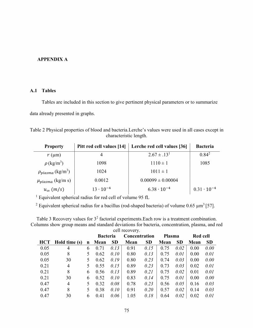
75

APPENDIX A

A.1 Tables

Tables are included in this section to give pertinent physical parameters or to summarize

data already presented in graphs.

Table 2 Physical properties of blood and bacteria.Lerche’s values were used in all cases except in

characteristic length.

Property Pitt red cell values [14] Lerche red cell values [36] Bacteria

𝑟 (µm) 4 2.67 ± .131 0.842

𝜌 (kg/m3) 1098 1110 ± 1 1085

𝜌𝑝𝑙𝑎𝑠𝑚𝑎 (kg/m3) 1024 1011 ± 1

𝜇𝑝𝑙𝑎𝑠𝑚𝑎 (kg/m s) 0.0012 0.00099 ± 0.00004

𝑢∞ (𝑚/𝑠) 13 ∙ 10−4 6.38 ∙ 10−4 0.31 ∙ 10−4

1 Equivalent spherical radius for red cell of volume 95 fL

2 Equivalent spherical radius for a bacillus (rod-shaped bacteria) of volume 0.65 µm3 [57].

Table 3 Recovery values for 32 factorial experiments.Each row is a treatment combination.

Columns show group means and standard deviations for bacteria, concentration, plasma, and red

cell recovery.

Bacteria Concentration Plasma Red cell

HCT Hold time (s) n Mean SD Mean SD Mean SD Mean SD

0.05 4 6 0.71 0.13 0.91 0.15 0.75 0.02 0.00 0.00

0.05 8 5 0.62 0.10 0.80 0.13 0.75 0.01 0.00 0.01

0.05 30 5 0.62 0.19 0.80 0.23 0.74 0.03 0.00 0.00

0.21 4 5 0.55 0.15 0.89 0.23 0.73 0.03 0.02 0.01

0.21 8 6 0.56 0.13 0.89 0.21 0.75 0.02 0.01 0.01

0.21 30 6 0.52 0.10 0.83 0.14 0.75 0.01 0.00 0.00

0.47 4 5 0.32 0.08 0.78 0.23 0.56 0.05 0.16 0.03

0.47 8 5 0.38 0.10 0.91 0.20 0.57 0.02 0.14 0.03

0.47 30 6 0.41 0.06 1.05 0.18 0.64 0.02 0.02 0.01

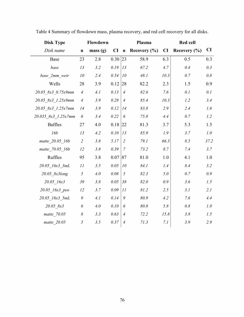
76

Table 4 Summary of flowdown mass, plasma recovery, and red cell recovery for all disks.

Disk Type

Disk name n

Flowdown

mass (g) CI n

Plasma

Recovery (%) CI

Red cell

Recovery (%) CI

Base 23 2.8 0.30 23 58.9 6.3 0.5 0.3

base 13 3.2 0.19 13 67.2 4.7 0.4 0.3

base_2mm_weir 10 2.4 0.54 10 48.1 10.3 0.7 0.8

Wells 28 3.9 0.12 28 82.2 2.3 1.5 0.9

20.05_8x3_0.75x9mm 4 4.1 0.13 4 82.6 7.6 0.1 0.1

20.05_8x3_1.25x9mm 4 3.9 0.28 4 85.4 10.3 1.2 3.4

20.05_8x3_1.25x7mm 14 3.9 0.12 14 83.8 2.9 2.4 1.6

20.035_8x3_1.25x7mm 6 3.4 0.22 6 75.8 4.4 0.7 1.2

Baffles 27 4.0 0.18 22 81.3 3.7 5.3 1.5

16b 13 4.2 0.10 13 85.9 1.9 3.7 1.0

matte_20.05_16b 2 3.8 5.17 2 79.1 66.3 8.5 37.2

matte_70.05_16b 12 3.8 0.39 7 73.2 8.7 7.4 3.7

Ruffles 95 3.8 0.07 87 81.0 1.0 4.1 1.0

20.05_16x3_3mL 11 3.5 0.05 10 84.1 1.4 8.4 3.2

20.05_8x3long 5 4.0 0.08 5 82.3 5.0 0.7 0.9

20.05_16x3 39 3.8 0.05 38 82.0 0.9 3.6 1.5

20.05_16x3_peo 12 3.7 0.09 11 81.2 2.5 3.1 2.1

20.05_16x3_5mL 9 4.1 0.14 9 80.9 4.2 7.6 4.4

20.05_8x3 6 4.0 0.10 6 80.8 5.8 0.8 1.0

matte_70.05 8 3.3 0.63 4 72.2 15.8 3.8 1.5

matte_20.05 5 3.5 0.37 4 71.3 7.1 3.9 2.9

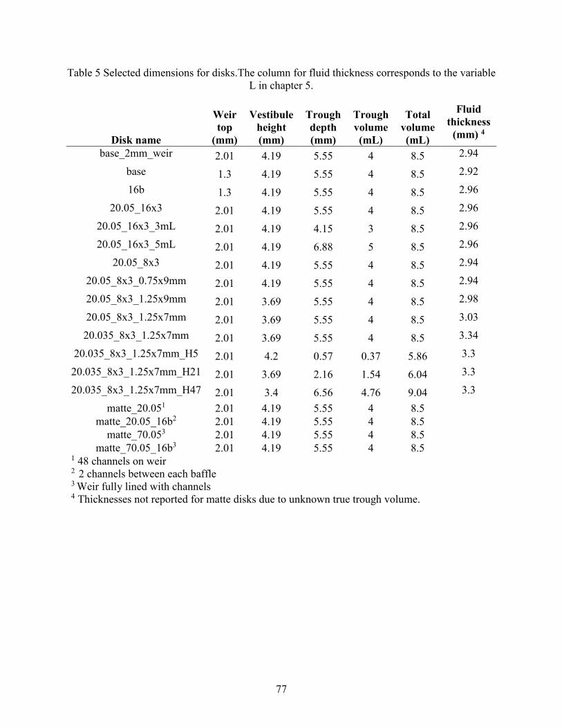
77

Table 5 Selected dimensions for disks.The column for fluid thickness corresponds to the variable

L in chapter 5.

Disk name

Weir

top

(mm)

Vestibule

height

(mm)

Trough

depth

(mm)

Trough

volume

(mL)

Total

volume

(mL)

Fluid

thickness

(mm) 4

base_2mm_weir 2.01 4.19 5.55 4 8.5 2.94

base 1.3 4.19 5.55 4 8.5 2.92

16b 1.3 4.19 5.55 4 8.5 2.96

20.05_16x3 2.01 4.19 5.55 4 8.5 2.96

20.05_16x3_3mL 2.01 4.19 4.15 3 8.5 2.96

20.05_16x3_5mL 2.01 4.19 6.88 5 8.5 2.96

20.05_8x3 2.01 4.19 5.55 4 8.5 2.94

20.05_8x3_0.75x9mm 2.01 4.19 5.55 4 8.5 2.94

20.05_8x3_1.25x9mm 2.01 3.69 5.55 4 8.5 2.98

20.05_8x3_1.25x7mm 2.01 3.69 5.55 4 8.5 3.03

20.035_8x3_1.25x7mm 2.01 3.69 5.55 4 8.5 3.34

20.035_8x3_1.25x7mm_H5 2.01 4.2 0.57 0.37 5.86 3.3

20.035_8x3_1.25x7mm_H21 2.01 3.69 2.16 1.54 6.04 3.3

20.035_8x3_1.25x7mm_H47 2.01 3.4 6.56 4.76 9.04 3.3

matte_20.051 2.01 4.19 5.55 4 8.5

matte_20.05_16b2 2.01 4.19 5.55 4 8.5

matte_70.053 2.01 4.19 5.55 4 8.5

matte_70.05_16b3 2.01 4.19 5.55 4 8.5

1 48 channels on weir 2 2 channels between each baffle 3 Weir fully lined with channels 4 Thicknesses not reported for matte disks due to unknown true trough volume.

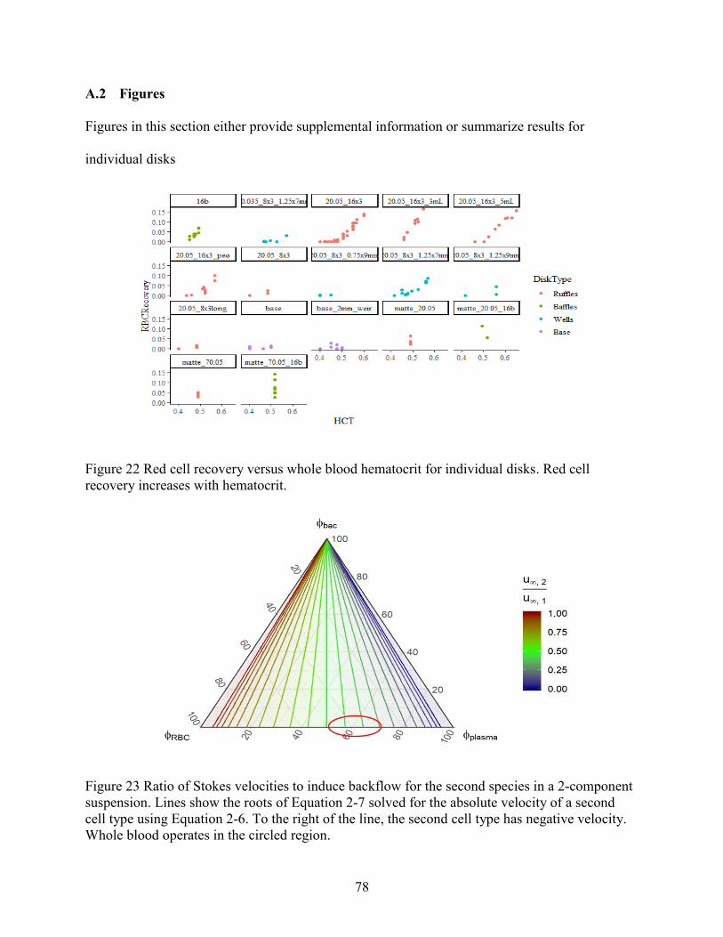
78

A.2 Figures

Figures in this section either provide supplemental information or summarize results for

individual disks

Figure 22 Red cell recovery versus whole blood hematocrit for individual disks. Red cell

recovery increases with hematocrit.

Figure 23 Ratio of Stokes velocities to induce backflow for the second species in a 2-component

suspension. Lines show the roots of Equation 2-7 solved for the absolute velocity of a second

cell type using Equation 2-6. To the right of the line, the second cell type has negative velocity.

Whole blood operates in the circled region.

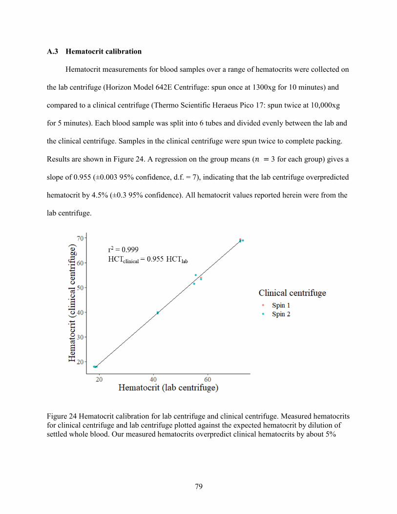
79

A.3 Hematocrit calibration

Hematocrit measurements for blood samples over a range of hematocrits were collected on

the lab centrifuge (Horizon Model 642E Centrifuge: spun once at 1300xg for 10 minutes) and

compared to a clinical centrifuge (Thermo Scientific Heraeus Pico 17: spun twice at 10,000xg

for 5 minutes). Each blood sample was split into 6 tubes and divided evenly between the lab and

the clinical centrifuge. Samples in the clinical centrifuge were spun twice to complete packing.

Results are shown in Figure 24. A regression on the group means (𝑛 = 3 for each group) gives a

slope of 0.955 (±0.003 95% confidence, d.f. = 7), indicating that the lab centrifuge overpredicted

hematocrit by 4.5% (±0.3 95% confidence). All hematocrit values reported herein were from the

lab centrifuge.

Figure 24 Hematocrit calibration for lab centrifuge and clinical centrifuge. Measured hematocrits

for clinical centrifuge and lab centrifuge plotted against the expected hematocrit by dilution of

settled whole blood. Our measured hematocrits overpredict clinical hematocrits by about 5%

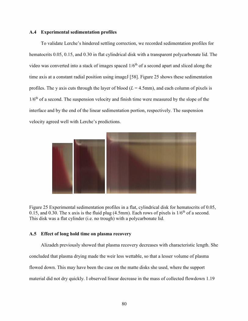
80

A.4 Experimental sedimentation profiles

To validate Lerche’s hindered settling correction, we recorded sedimentation profiles for

hematocrits 0.05, 0.15, and 0.30 in flat cylindrical disk with a transparent polycarbonate lid. The

video was converted into a stack of images spaced 1/6th of a second apart and sliced along the

time axis at a constant radial position using imageJ [58]. Figure 25 shows these sedimentation

profiles. The y axis cuts through the layer of blood (L = 4.5mm), and each column of pixels is

1/6th of a second. The suspension velocity and finish time were measured by the slope of the

interface and by the end of the linear sedimentation portion, respectively. The suspension

velocity agreed well with Lerche’s predictions.

Figure 25 Experimental sedimentation profiles in a flat, cylindrical disk for hematocrits of 0.05,

0.15, and 0.30. The x axis is the fluid plug (4.5mm). Each rows of pixels is 1/6th of a second.

This disk was a flat cylinder (i.e. no trough) with a polycarbonate lid.

A.5 Effect of long hold time on plasma recovery

Alizadeh previously showed that plasma recovery decreases with characteristic length. She

concluded that plasma drying made the weir less wettable, so that a lesser volume of plasma

flowed down. This may have been the case on the matte disks she used, where the support

material did not dry quickly. I observed linear decrease in the mass of collected flowdown 1.19

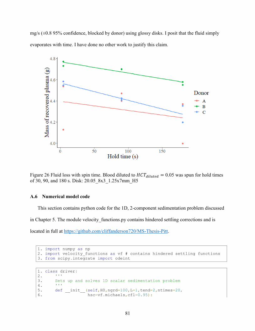
81

mg/s (±0.8 95% confidence, blocked by donor) using glossy disks. I posit that the fluid simply

evaporates with time. I have done no other work to justify this claim.

Figure 26 Fluid loss with spin time. Blood diluted to 𝐻𝐶𝑇𝑑𝑖𝑙𝑢𝑡𝑒𝑑 = 0.05 was spun for hold times

of 30, 90, and 180 s. Disk: 20.05_8x3_1.25x7mm_H5

A.6 Numerical model code

This section contains python code for the 1D, 2-component sedimentation problem discussed

in Chapter 5. The module velocity_functions.py contains hindered settling corrections and is

located in full at https://github.com/cliffanderson720/MS-Thesis-Pitt.

1. import numpy as np 2. import velocity_functions as vf # contains hindered settling functions 3. from scipy.integrate import odeint

1. class driver: 2. ''' 3. Sets up and solves 1D scalar sedimentation problem 4. ''' 5. def __init__(self,H0,ngrd=100,L=1,tend=2,ntimes=20, 6. hsc=vf.michaels,cfl=0.95):

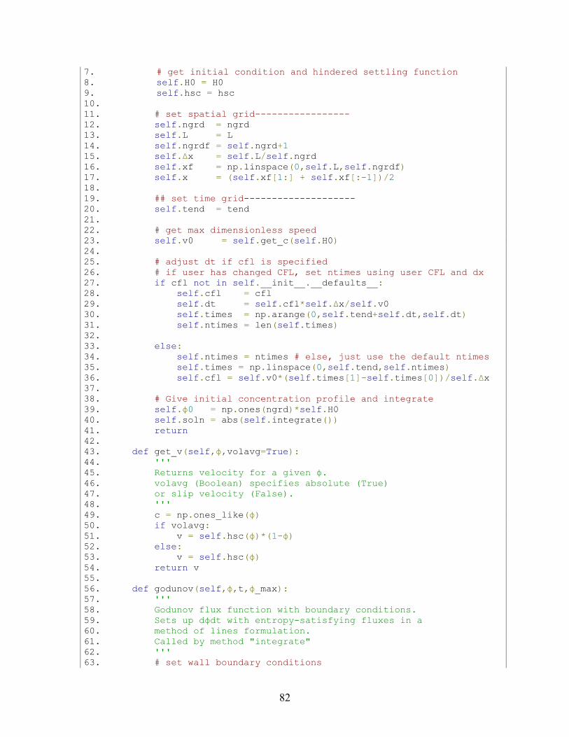
82

7. # get initial condition and hindered settling function 8. self.H0 = H0 9. self.hsc = hsc 10.

11. # set spatial grid-----------------

12. self.ngrd = ngrd

13. self.L = L

14. self.ngrdf = self.ngrd+1

15. self.Δx = self.L/self.ngrd

16. self.xf = np.linspace(0,self.L,self.ngrdf)

17. self.x = (self.xf[1:] + self.xf[:-1])/2

18.

19. ## set time grid--------------------

20. self.tend = tend

21.

22. # get max dimensionless speed

23. self.v0 = self.get_c(self.H0)

24.

25. # adjust dt if cfl is specified

26. # if user has changed CFL, set ntimes using user CFL and dx

27. if cfl not in self.__init__.__defaults__:

28. self.cfl = cfl

29. self.dt = self.cfl*self.Δx/self.v0

30. self.times = np.arange(0,self.tend+self.dt,self.dt)

31. self.ntimes = len(self.times)

32.

33. else:

34. self.ntimes = ntimes # else, just use the default ntimes

35. self.times = np.linspace(0,self.tend,self.ntimes)

36. self.cfl = self.v0*(self.times[1]-self.times[0])/self.Δx

37.

38. # Give initial concentration profile and integrate

39. self.ϕ0 = np.ones(ngrd)*self.H0

40. self.soln = abs(self.integrate())

41. return

42.

43. def get_v(self,ϕ,volavg=True):

44. '''

45. Returns velocity for a given ϕ.

46. volavg (Boolean) specifies absolute (True)

47. or slip velocity (False).

48. '''

49. c = np.ones_like(ϕ)

50. if volavg:

51. v = self.hsc(ϕ)*(1-ϕ)

52. else:

53. v = self.hsc(ϕ)

54. return v

55.

56. def godunov(self,ϕ,t,ϕ_max):

57. '''

58. Godunov flux function with boundary conditions.

59. Sets up dϕdt with entropy-satisfying fluxes in a

60. method of lines formulation.

61. Called by method "integrate"

62. '''

63. # set wall boundary conditions

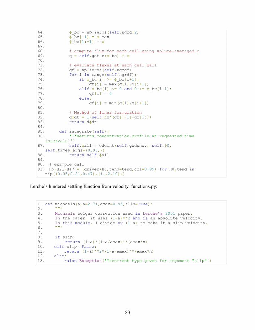
83

64. ϕ_bc = np.zeros(self.ngrd+2)

65. ϕ_bc[-1] = ϕ_max

66. ϕ_bc[1:-1] = ϕ

67.

68. # compute flux for each cell using volume-averaged ϕ

69. q = self.get_c(ϕ_bc) * ϕ

70.

71. # evaluate fluxes at each cell wall

72. qf = np.zeros(self.ngrdf)

73. for i in range(self.ngrdf):

74. if ϕ_bc[i] >= ϕ_bc[i+1]:

75. qf[i] = max(q[i],q[i+1])

76. elif ϕ_bc[i] <= 0 and 0 <= ϕ_bc[i+1]:

77. qf[i] = 0

78. else:

79. qf[i] = min(q[i],q[i+1])

80.

81. # Method of lines formulation

82. dϕdt = 1/self.Δx*(qf[:-1]-qf[1:])

83. return dϕdt

84.

85. def integrate(self):

86. '''Returns concentration profile at requested time

intervals'''

87. self.ϕall = odeint(self.godunov, self.ϕ0,

self.times,args=(0.95,))

88. return self.ϕall

89.

90. # example call

91. H5,H21,H47 = [driver(H0,tend=tend,cfl=0.99) for H0,tend in

zip((0.05,0.21,0.47),(1.,2,10))]

Lerche’s hindered settling function from velocity_functions.py:

1. def michaels(a,n=2.71,amax=0.95,slip=True): 2. “”” 3. Michaels bolger correction used in Lerche’s 2001 paper. 4. In the paper, it uses (1-a)**2 and is an absolute velocity. 5. In this module, I divide by (1-a) to make it a slip velocity. 6. “”” 7. 8. if slip: 9. return (1-a)*(1-a/amax)**(amax*n) 10. elif slip==False:

11. return (1-a)**2*(1-a/amax)**(amax*n)

12. else:

13. raise Exception('Incorrect type given for argument "slip"')