Improving Calibration for Long-Tailed Recognition

Improving Calibration for Long-Tailed Recognition

Zhisheng Zhong Jiequan Cui Shu Liu Jiaya JiaChinese University of Hong Kong SmartMoreCode: https://github.com/Jia-Research-Lab/MiSLAS

Abstract

Deep neural networks may perform poorly when train-ing datasets are heavily class-imbalanced. Recently, two-stage methods decouple representation learning and classi-fier learning to improve performance. But there is still thevital issue of miscalibration. To address it, we design twomethods to improve calibration and performance in suchscenarios. Motivated by the fact that predicted probabilitydistributions of classes are highly related to the numbers ofclass instances, we propose label-aware smoothing to dealwith different degrees of over-confidence for classes and im-prove classifier learning. For dataset bias between thesetwo stages due to different samplers, we further proposeshifted batch normalization in the decoupling framework.Our proposed methods set new records on multiple popu-lar long-tailed recognition benchmark datasets, includingCIFAR-10-LT, CIFAR-100-LT, ImageNet-LT, Places-LT, andiNaturalist 2018.

1. Introduction

With numerous available large-scale and high-qualitydatasets, such as ImageNet [27], COCO [19], andPlaces [40], deep convolutional neural networks (CNNs)have made notable breakthrough in various computer vi-sion tasks, such as image recognition [16, 10], object detec-tion [26], and semantic segmentation [6]. These datasetsare usually artificially balanced with respect to the numberof instances for each object/class. However, in many real-world applications, data may follow unexpected long-taileddistributions, where the numbers of instances for differentclasses are seriously imbalanced. When training CNNs onthese long-tailed datasets, the performance notably degrades.To address this terrible issue, a number of methods wereproposed for long-tailed recognition.

Recently, many two-stage approaches have achievedsignificant improvement comparing with one-stage meth-ods. Deferred re-sampling (DRS, [4]) and deferred re-weighting (DRW, [4]) first train CNNs in a normal way inStage-1. DRS tunes CNNs on datasets with class-balanced

Org. CIFAR-100 CIFAR-100-LT, IF100

0.0 0.2 0.4 0.6 0.8 1.0

0.2

0.4

0.6

0.8

1.0

Accu

racy

ACC=70.7%ECE=12.2%

GapAccuracy

0.0 0.2 0.4 0.6 0.8 1.0

ACC=39.0%ECE=38.1%

GapAccuracy

ConfidenceCIFAR-100-LT, IF100, cRT CIFAR-100-LT, IF100, LWS

0.0 0.2 0.4 0.6 0.8 1.0

0.2

0.4

0.6

0.8

1.0

Accu

racy

ACC=40.7%ECE=29.5%

GapAccuracy

0.0 0.2 0.4 0.6 0.8 1.0

ACC=41.2%ECE=36.3%

GapAccuracy

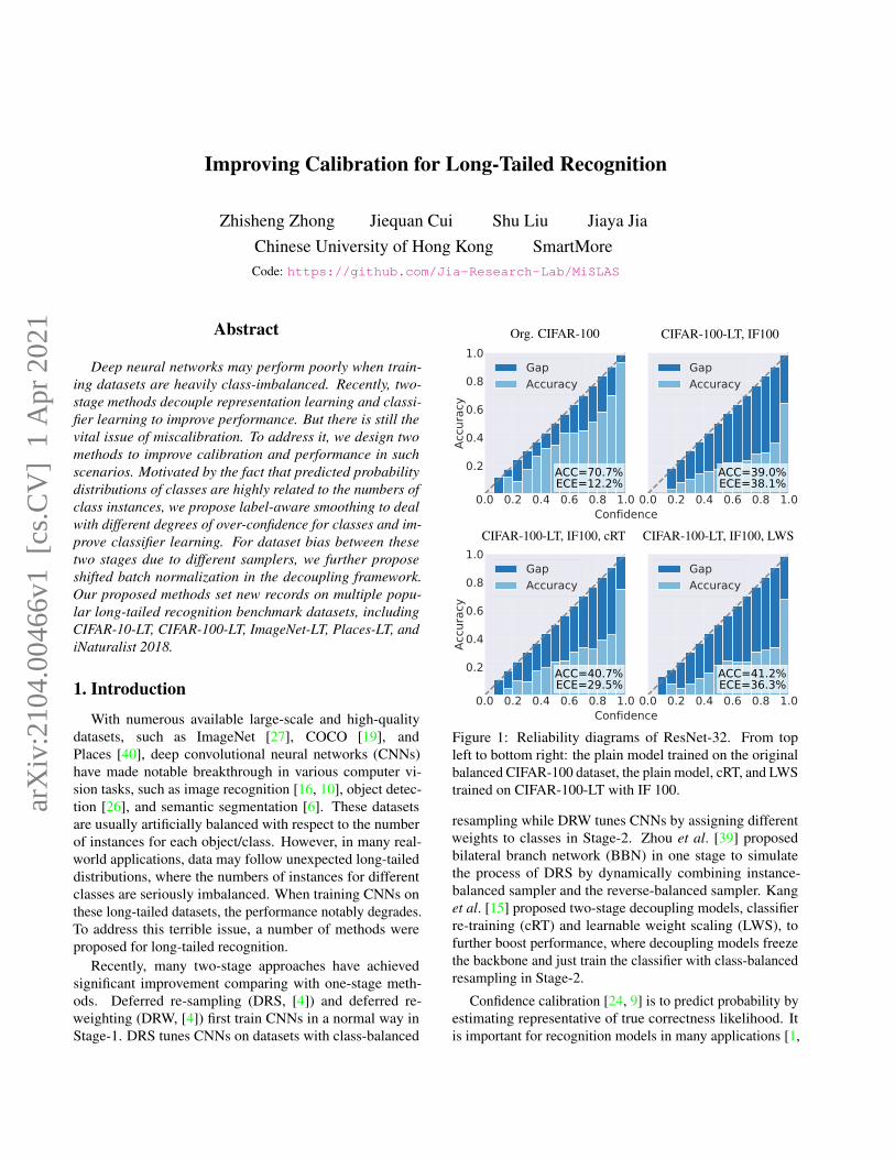
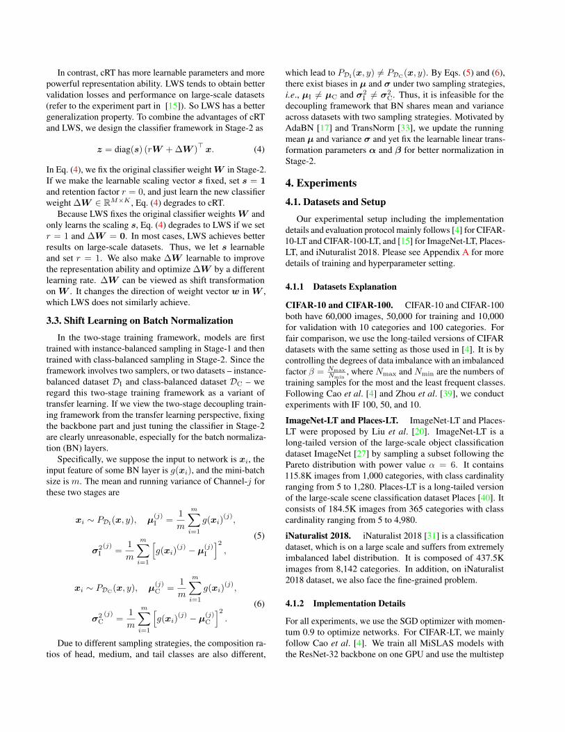
ConfidenceFigure 1: Reliability diagrams of ResNet-32. From topleft to bottom right: the plain model trained on the originalbalanced CIFAR-100 dataset, the plain model, cRT, and LWStrained on CIFAR-100-LT with IF 100.

resampling while DRW tunes CNNs by assigning differentweights to classes in Stage-2. Zhou et al. [39] proposedbilateral branch network (BBN) in one stage to simulatethe process of DRS by dynamically combining instance-balanced sampler and the reverse-balanced sampler. Kanget al. [15] proposed two-stage decoupling models, classifierre-training (cRT) and learnable weight scaling (LWS), tofurther boost performance, where decoupling models freezethe backbone and just train the classifier with class-balancedresampling in Stage-2.

Confidence calibration [24, 9] is to predict probability byestimating representative of true correctness likelihood. Itis important for recognition models in many applications [1,

arX

iv:2

104.

0046

6v1

[cs

.CV

] 1

Apr

202

1

https://github.com/Jia-Research-Lab/MiSLAS

14]. Expected calibration error (ECE) is widely used inmeasuring calibration of the network. To compute ECE, allN predictions are first grouped into B interval bins of equalsize. ECE is defined as:

ECE =

B∑b=1

|Sb|N

∣∣∣∣acc(Sb)− conf(Sb)∣∣∣∣× 100%,

where Sb is the set of samples whose prediction scores fallinto Bin-b. acc(·) and conf(·) are the accuracy and predictedconfidence of Sb, respectively.

Our study shows, because of the imbalanced compositionratio of each class, networks trained on long-tailed datasetsare more miscalibrated and over-confident. We draw thereliability diagrams with 15 bins in Fig. 1, which comparesthe plain cross-entropy (CE) model trained on the originalCIFAR-100 dataset, the plain CE model, cRT, and LWStrained on CIFAR-100-LT with imbalanced factor (IF) 100.It is noticeable that networks trained on long-tailed datasetsusually have higher ECEs. The two-stage models of cRTand LWS suffer from over-confidence as well. Moreover,Figs. 9 and 10 (the first two plots) in Appendix C depict thatthis phenomenon also commonly exists on other long-taileddatasets, such as CIFAR-10-LT and ImageNet-LT.

Another issue is that two-stage decoupling ignores thedataset bias or domain shift [25] in the two stages. In de-tails, two-stage models are first trained on the instanced-balanced dataset DI in Stage-1. Then, models are trainedon the class-balanced dataset DC in Stage-2. Obviously,PDI

(x, y) 6= PDC(x, y) and distributions of the dataset

by different sampling ways are inconsistent. Motivated bytransfer learning [17, 33], we focus on the batch normaliza-tion [12] layer to deal with the dataset bias problem.

In this work, we propose a Mixup Shifted Label-AwareSmoothing model (MiSLAS) to effectively solve above is-sues. Our key contributions are as follows.

• We discover that models trained on long-tailed datasets aremuch more miscalibrated and over-confident than thosetrained on balanced data. Two-stage models suffer fromthis problem as well.

• We find that mixup can remedy over-confidence and havea positive effect on representation learning but a nega-tive or negligible effect on classifier learning. To furtherenhance classifier learning and calibration, we proposelabel-aware smoothing to handle different degrees of over-confidence for classes.

• It is the first attempt to note the dataset bias or domain shiftin two-stage resampling methods for long-tailed recog-nition. To deal with it in the decoupling framework, wepropose shift learning on the batch normalization layer,which can greatly improve performance.

• We extensively validate our MiSLAS on multiple long-tailed recognition benchmark datasets – experimental re-sults manifest the effectiveness. Our method yields newstate-of-the-art.

2. Related Work

Re-sampling and re-weighting. There are two groupsof re-sampling strategies: over-sampling the tail-class im-ages [28, 2, 3] and under-sampling the head-class im-ages [13, 2]. Over-sampling is regularly useful on largedatasets and may suffer from heavy over-fitting to tail classesespecially on small datasets. For under-sampling, it dis-cards a large portion of data, which inevitably causes degra-dation of the generalization ability of deep models. Re-weighting [11, 34] is another prominent strategy. It assignsdifferent weights for classes and even instances. The vanillare-weighting method gives class weights in reverse propor-tion to the number of samples of classes.

However, with large-scale data, re-weighting makes deepmodels difficult to optimize during training. Cui et al. [7]relieved the problem using the effective numbers to calculatethe class weights. Another line of work is to adaptivelyre-weight each instance. For example, focal loss [18, 22]assigned smaller weights for well-classified samples.

Confidence calibration and regularization. Calibratedconfidence is significant for classification models in manyapplications. Calibration of modern neural networks is firstdiscussed in [9]. The authors discovered that model capacity,normalization, and regularization have strong effect on net-work calibration. mixup [37] is a regularization technique totrain with interpolation of input and labels.

mixup inspires follow-up of manifold mixup [32], Cut-Mix [36], and Remix [5] that have shown significant im-provement. Thulasidasan et al. [30] found that CNNs trainedwith mixup are better calibrated. Label smoothing [29] is an-other regularization technique that encourages the model tobe less over-confident. Unlike cross-entropy that computesloss upon the ground truth labels, label smoothing computesloss upon a soft version of labels. It relieves over-fitting andincreases calibration and reliability [23].

Two-stage methods. Cao et al. [4] proposed deferred re-weighting (DRW) and deferred re-sampling (DRS), workingbetter than conventional one-stage methods. Its stage-2, start-ing from better features, adjusts the decision boundary andlocally tunes features. Recently, Kang et al. [15] and Zhouet al. [39] concluded that although class re-balance mattersfor jointly training representation and classifier, instance-balanced sampling gives more general representations.

Based on this observation, Kang et al. [15] achievedstate-of-the-art results by decomposing representation andclassifier learning. It first trains the deep models with

Mark Stg.-1 Stg.-2 ResNet-50 ResNet-101 ResNet-152

CE 8� 45.7 / 13.7 47.3 / 13.7 48.7 / 14.5CE 4� 45.5 / 7.98 47.7 / 10.1 48.3 / 10.2

cRT 8� 8� 50.3 / 8.97 51.3 / 9.34 52.7 / 9.05cRT 8� 4� 50.2 / 3.32 51.3 / 3.38 52.8 / 3.60cRT 4� 8� 51.7 / 5.62 53.1 / 6.86 54.2 / 6.02cRT 4� 4� 51.6 / 3.13 53.0 / 2.93 54.1 / 3.37

Mark Stg.-1 Stg.-2 ResNet-50 ResNet-101 ResNet-152

CE 8� 45.7 / 13.7 47.3 / 13.7 48.7 / 14.5CE 4� 45.5 / 7.98 47.7 / 10.1 48.3 / 10.2

LWS 8� 8� 51.2 / 4.89 52.3 / 5.10 53.8 / 4.48LWS 8� 4� 51.0 / 5.01 52.2 / 5.38 53.6 / 5.50LWS 4� 8� 52.0 / 2.23 53.5 / 2.73 54.6 / 2.46LWS 4� 4� 52.0 / 8.04 53.3 / 6.97 54.4 / 7.74

Table 1: Top-1 accuracy (%) and ECE (%) of the plain cross-entropy (CE) model, and decoupling models of cRT (left) andLWS (right), for ResNet families trained on the ImageNet-LT dataset. We vary the augmentation strategies with ( 4�), or without( 8�) mixup α = 0.2, on both of the stages.

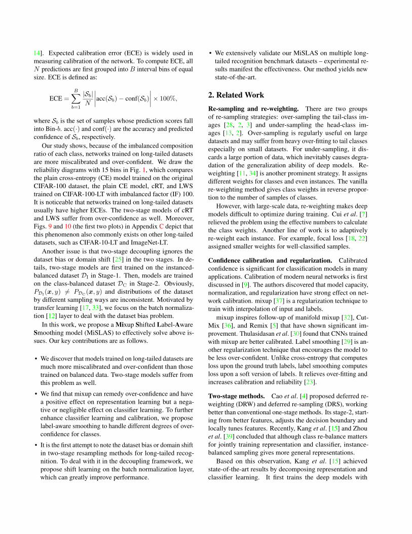
Figure 2: Classifier weight norms for the ImageNet-LT validation set where classes are sorted by descending values of Nj ,where Nj denotes the number of training sample for Class-j. Left: weight norms of cRT with or without mixup. Right: weightnorms of LWS with or without mixup. Light shade: true norm. Dark lines: smooth version. Best viewed on screen.

instance-balanced sampling, and then fine-tunes the clas-sifier with class-balanced sampling with parameters of rep-resentation learning fixed. Similarly, Zhou et al. [39] inte-grated mixup training into the proposed cumulative learningstrategy. It bridges the representation learning and classi-fier re-balancing. The cumulative learning strategy requiresdual samplers of instance-balanced and reversed instance-balanced sampler.

3. Main Approach3.1. Study of mixup Strategy

For the two-stage learning framework, Kang et al. [15]and Zhou et al. [39] found that instance-balanced samplinggives the most general representation among all for long-tailed recognition. Besides, Thulasidasan et al. [30] showthat networks trained with mixup are better calibrated. Basedon these findings, when using instance-balanced sampling,we explore the effect of mixup in the two-stage decouplingframework for higher representation generalization and over-confidence reduction.

We train a plain cross-entropy model, and two two-stagemodels of cRT and LWS, on ImageNet-LT for 180 epochsin Stage-1 and finetune them for 10 epochs in Stage-2, re-spectively. We vary the training setup (with/without mixup

α = 0.2) for both stages. Top-1 accuracy of these variantsis listed in Table 1. It reveals the following. (i) When ap-plying mixup, improvement of CE can be ignored. But theperformance is greatly enhanced for both cRT and LWS.(ii) Applying additional mixup in Stage-2 yields no obviousimprovement or even damages performance. The reasonis that mixup encourages representation learning and is yetwith adverse or negligible effect on classifier learning.

Besides, we draw the final classifier weight norms ofthese variants in Fig. 2. We show the L2 norms of the weightvectors for all classes, as well as the training data distributionsorted in a descending manner concerning the number ofinstances. We observe that when applying mixup (in orange),the weight norms of the tail classes tends to be large and theweight norms of the head classes decrease. It means mixupmay be more friendly to tail classes.

We also list ECEs of the above models in Table 1. Whenadding mixup in just Stage-1, both cRT and LWS models canconsistently obtain better top-1 accuracy and lower ECEsfor different backbones (Row-4 and Row-6). Due to theunsatisfied top-1 accuracy enhancement and unstable ECEdecline of mixup for classifier learning (by adding mixupin Stage-2), we propose a label-aware smoothing to furtherimprove both calibration and classifier learning.

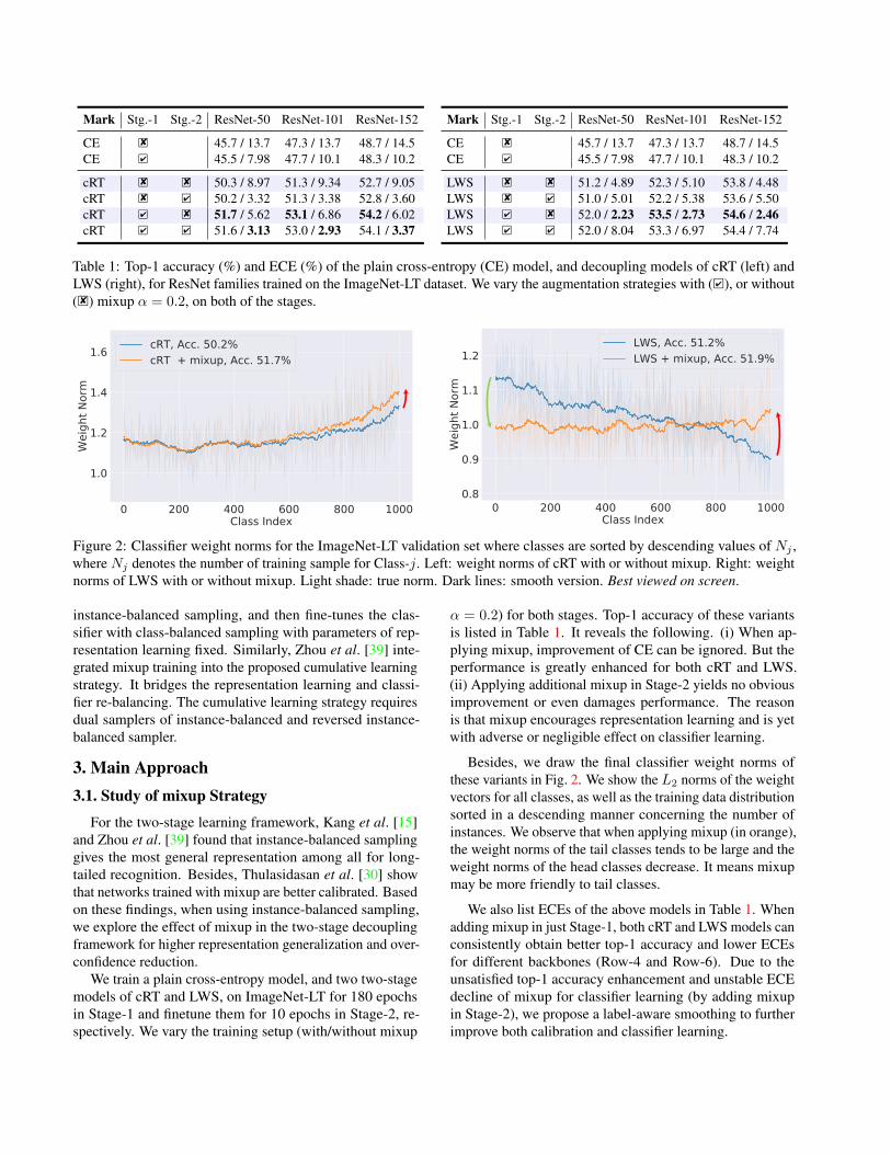
Figure 3: Violin plot of predicted probability distributions for different parts of the classes, head (100+ images per class),medium (20-100 images per class), and tail (less than 20 images per class) on CIFAR-100-LT with IF 100. The upper half partin light blue denotes “LWS + cross-entropy”. The bottom half part in deep blue represents “LWS + label-aware smoothing”.

3.2. Label-aware Smoothing

In this subsection, we analyze and deal with the two issuesof over-confidence and limited improvement by classifierlearning. Suppose weight of the classifier is W ∈ RM×K ,where M is the number of features and K is the number ofclasses. The cross-entropy encourages the whole networkto be over-confident on the head classes. The cross-entropyloss after the softmax activation is l(y,p) = − log(py) =

−w>y x + log(∑

exp(w>i x)), where y ∈ {1, 2, ...,K} isthe label. x ∈ RM is the feature vector send to classifier andwi is the i-th column vector ofW . The optimal solution isw∗y>x = inf , while other w>i x, i 6= y are small enough.Because the head classes contain much more training ex-

amples, the network makes the weight norm ‖w‖ of the headclasses larger to approach the optimal solution. It resultsin predicted probabilities mainly near 1.0 (see Fig. 3, theupper half in light blue). Another fact is that distributions ofpredicted probability are related to instance numbers. Unlikebalanced recognition, applying different strategies for theseclasses is necessary for solving the long-tailed problem.

Here, we propose label-aware smoothing to solve theover-confidence in cross-entropy and varying distributionsof predicted probability issues. It is expressed as

l(q,p) = −K∑i=1

qi log pi,

qi =

{1− εy = 1− f(Ny), i = y,εyK−1 =

f(Ny)K−1 , otherwise,

(1)

where εy is a small label smoothing factor for Class-y, re-lating to its class number Ny. Now the optimal solutionbecomes (proof presented in Appendix E)

w∗i>x =

{log(

(K−1)(1−εy)εy

)+ c, i = y,

c, otherwise,(2)

where c is an arbitrary real number. Compared with the

optimal solution in cross-entropy, the label-aware smoothingencourages a finite output, more general and remedyingoverfit. We suppose the labels of the long-tailed datasetare assigned in a descending order concerning the numberof instances, i.e., N1 ≥ N2 ≥ ... ≥ NK . Because thehead classes contain more diverse examples, the predictedprobabilities are more promising than those of tail classes.Thus, we require the classes with larger instance numbers tobe penalized with stronger label smoothing factors – that is,the related function f(Ny) should be negatively correlatedto Ny . We define three types of related function f(Ny) as

• Concave form:

f(Ny) = εK + (ε1 − εK) sin

[π(Ny −NK)

2(N1 −NK)

]; (3.a)

• Linear form:

f(Ny) = εK + (ε1 − εK)Ny −NKN1 −NK

; (3.b)

• Convex form:

f(Ny) = ε1+(ε1−εK) sin

[3π

2+π(Ny −NK)

2(N1 −NK)

], (3.c)

where ε1 and εK are two hyperparameters. Illustration ofthese functions is shown in Fig. 6. If we set ε1 ≥ εK ,ε1 ≥ ε2 ≥ ... ≥ εK is obtained. For large instance numberNy for Class-y, label-aware smoothing allocates a strongsmoothing factor. It lowers the fitting probability to relieveover-confidence because the head and medium classes aremore likely to be over-confident than the tail classes (seeFig. 3).

As the form of label-aware smoothing is more compli-cated than cross-entropy, we propose a generalized classifierlearning framework to fit it. Here we give a quick reviewabout cRT and LWS. cRT learns a classifier weight, whichcontains KM learnable parameters, while LWS is restrictedto learning the weight scaling vector s ∈ RK with only Klearnable parameters.

In contrast, cRT has more learnable parameters and morepowerful representation ability. LWS tends to obtain bettervalidation losses and performance on large-scale datasets(refer to the experiment part in [15]). So LWS has a bettergeneralization property. To combine the advantages of cRTand LWS, we design the classifier framework in Stage-2 as

z = diag(s) (rW + ∆W )>x. (4)

In Eq. (4), we fix the original classifier weightW in Stage-2.If we make the learnable scaling vector s fixed, set s = 1and retention factor r = 0, and just learn the new classifierweight ∆W ∈ RM×K , Eq. (4) degrades to cRT.

Because LWS fixes the original classifier weightsW andonly learns the scaling s, Eq. (4) degrades to LWS if we setr = 1 and ∆W = 0. In most cases, LWS achieves betterresults on large-scale datasets. Thus, we let s learnableand set r = 1. We also make ∆W learnable to improvethe representation ability and optimize ∆W by a differentlearning rate. ∆W can be viewed as shift transformationon W . It changes the direction of weight vector w in W ,which LWS does not similarly achieve.

3.3. Shift Learning on Batch Normalization

In the two-stage training framework, models are firsttrained with instance-balanced sampling in Stage-1 and thentrained with class-balanced sampling in Stage-2. Since theframework involves two samplers, or two datasets – instance-balanced dataset DI and class-balanced dataset DC – weregard this two-stage training framework as a variant oftransfer learning. If we view the two-stage decoupling train-ing framework from the transfer learning perspective, fixingthe backbone part and just tuning the classifier in Stage-2are clearly unreasonable, especially for the batch normaliza-tion (BN) layers.

Specifically, we suppose the input to network is xi, theinput feature of some BN layer is g(xi), and the mini-batchsize is m. The mean and running variance of Channel-j forthese two stages are

xi ∼ PDI(x, y), µ(j)I =

1

m

m∑i=1

g(xi)(j),

σ2I(j)

=1

m

m∑i=1

[g(xi)

(j) − µ(j)I

]2,

(5)

xi ∼ PDC(x, y), µ(j)C =

1

m

m∑i=1

g(xi)(j),

σ2C(j)

=1

m

m∑i=1

[g(xi)

(j) − µ(j)C

]2.

(6)

Due to different sampling strategies, the composition ra-tios of head, medium, and tail classes are also different,

which lead to PDI(x, y) 6= PDC(x, y). By Eqs. (5) and (6),there exist biases in µ and σ under two sampling strategies,i.e., µI 6= µC and σ2

I 6= σ2C. Thus, it is infeasible for the

decoupling framework that BN shares mean and varianceacross datasets with two sampling strategies. Motivated byAdaBN [17] and TransNorm [33], we update the runningmean µ and variance σ and yet fix the learnable linear trans-formation parameters α and β for better normalization inStage-2.

4. Experiments

4.1. Datasets and Setup

Our experimental setup including the implementationdetails and evaluation protocol mainly follows [4] for CIFAR-10-LT and CIFAR-100-LT, and [15] for ImageNet-LT, Places-LT, and iNuturalist 2018. Please see Appendix A for moredetails of training and hyperparameter setting.

4.1.1 Datasets Explanation

CIFAR-10 and CIFAR-100. CIFAR-10 and CIFAR-100both have 60,000 images, 50,000 for training and 10,000for validation with 10 categories and 100 categories. Forfair comparison, we use the long-tailed versions of CIFARdatasets with the same setting as those used in [4]. It is bycontrolling the degrees of data imbalance with an imbalancedfactor β = Nmax

Nmin, where Nmax and Nmin are the numbers of

training samples for the most and the least frequent classes.Following Cao et al. [4] and Zhou et al. [39], we conductexperiments with IF 100, 50, and 10.

ImageNet-LT and Places-LT. ImageNet-LT and Places-LT were proposed by Liu et al. [20]. ImageNet-LT is along-tailed version of the large-scale object classificationdataset ImageNet [27] by sampling a subset following thePareto distribution with power value α = 6. It contains115.8K images from 1,000 categories, with class cardinalityranging from 5 to 1,280. Places-LT is a long-tailed versionof the large-scale scene classification dataset Places [40]. Itconsists of 184.5K images from 365 categories with classcardinality ranging from 5 to 4,980.

iNaturalist 2018. iNaturalist 2018 [31] is a classificationdataset, which is on a large scale and suffers from extremelyimbalanced label distribution. It is composed of 437.5Kimages from 8,142 categories. In addition, on iNaturalist2018 dataset, we also face the fine-grained problem.

4.1.2 Implementation Details

For all experiments, we use the SGD optimizer with momen-tum 0.9 to optimize networks. For CIFAR-LT, we mainlyfollow Cao et al. [4]. We train all MiSLAS models withthe ResNet-32 backbone on one GPU and use the multistep

mixup + cRT mixup + LWS mixup + LWS + shifted BN MiSLAS

0.0 0.2 0.4 0.6 0.8 1.0

0.2

0.4

0.6

0.8

1.0

Accu

racy

ACC=45.2%ECE=13.8%

GapAccuracy

0.0 0.2 0.4 0.6 0.8 1.0

ACC=44.2%ECE=22.5%

GapAccuracy

0.0 0.2 0.4 0.6 0.8 1.0

ACC=45.3%ECE=22.2%

GapAccuracy

0.0 0.2 0.4 0.6 0.8 1.0

ACC=47.0%ECE=4.83%

GapAccuracy

Confidence

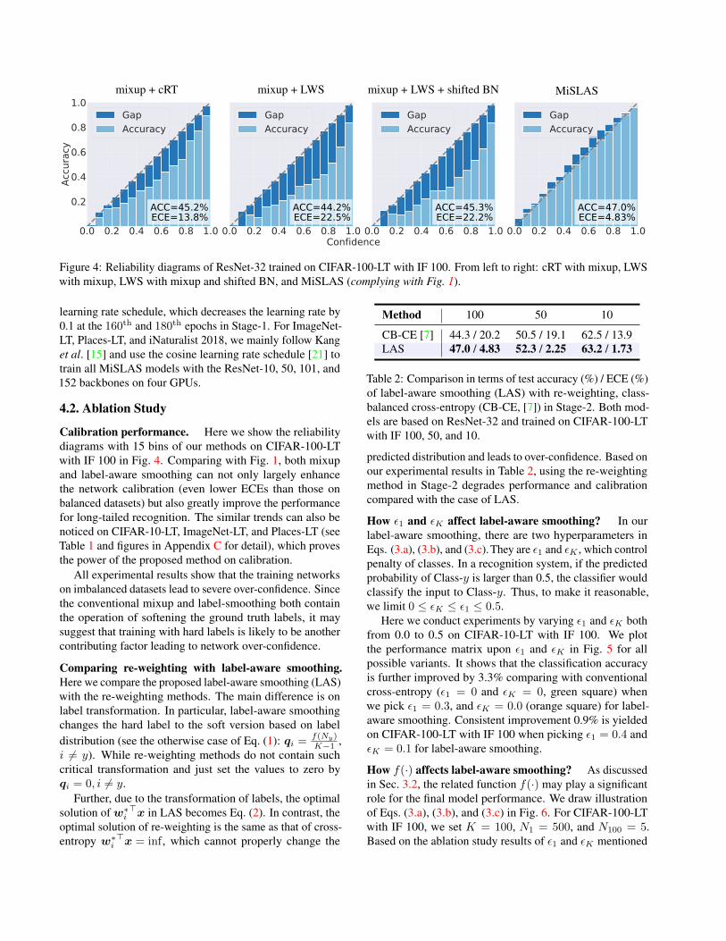
Figure 4: Reliability diagrams of ResNet-32 trained on CIFAR-100-LT with IF 100. From left to right: cRT with mixup, LWSwith mixup, LWS with mixup and shifted BN, and MiSLAS (complying with Fig. 1).

learning rate schedule, which decreases the learning rate by0.1 at the 160th and 180th epochs in Stage-1. For ImageNet-LT, Places-LT, and iNaturalist 2018, we mainly follow Kanget al. [15] and use the cosine learning rate schedule [21] totrain all MiSLAS models with the ResNet-10, 50, 101, and152 backbones on four GPUs.

4.2. Ablation Study

Calibration performance. Here we show the reliabilitydiagrams with 15 bins of our methods on CIFAR-100-LTwith IF 100 in Fig. 4. Comparing with Fig. 1, both mixupand label-aware smoothing can not only largely enhancethe network calibration (even lower ECEs than those onbalanced datasets) but also greatly improve the performancefor long-tailed recognition. The similar trends can also benoticed on CIFAR-10-LT, ImageNet-LT, and Places-LT (seeTable 1 and figures in Appendix C for detail), which provesthe power of the proposed method on calibration.

All experimental results show that the training networkson imbalanced datasets lead to severe over-confidence. Sincethe conventional mixup and label-smoothing both containthe operation of softening the ground truth labels, it maysuggest that training with hard labels is likely to be anothercontributing factor leading to network over-confidence.

Comparing re-weighting with label-aware smoothing.Here we compare the proposed label-aware smoothing (LAS)with the re-weighting methods. The main difference is onlabel transformation. In particular, label-aware smoothingchanges the hard label to the soft version based on labeldistribution (see the otherwise case of Eq. (1): qi =

f(Ny)K−1 ,

i 6= y). While re-weighting methods do not contain suchcritical transformation and just set the values to zero byqi = 0, i 6= y.

Further, due to the transformation of labels, the optimalsolution ofw∗i

>x in LAS becomes Eq. (2). In contrast, theoptimal solution of re-weighting is the same as that of cross-entropy w∗i

>x = inf , which cannot properly change the

Method 100 50 10

CB-CE [7] 44.3 / 20.2 50.5 / 19.1 62.5 / 13.9LAS 47.0 / 4.83 52.3 / 2.25 63.2 / 1.73

Table 2: Comparison in terms of test accuracy (%) / ECE (%)of label-aware smoothing (LAS) with re-weighting, class-balanced cross-entropy (CB-CE, [7]) in Stage-2. Both mod-els are based on ResNet-32 and trained on CIFAR-100-LTwith IF 100, 50, and 10.

predicted distribution and leads to over-confidence. Based onour experimental results in Table 2, using the re-weightingmethod in Stage-2 degrades performance and calibrationcompared with the case of LAS.

How ε1 and εK affect label-aware smoothing? In ourlabel-aware smoothing, there are two hyperparameters inEqs. (3.a), (3.b), and (3.c). They are ε1 and εK , which controlpenalty of classes. In a recognition system, if the predictedprobability of Class-y is larger than 0.5, the classifier wouldclassify the input to Class-y. Thus, to make it reasonable,we limit 0 ≤ εK ≤ ε1 ≤ 0.5.

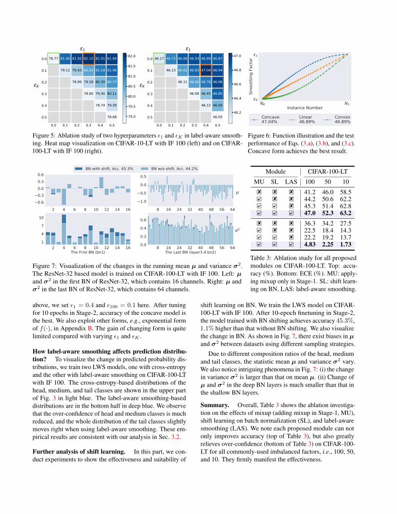
Here we conduct experiments by varying ε1 and εK bothfrom 0.0 to 0.5 on CIFAR-10-LT with IF 100. We plotthe performance matrix upon ε1 and εK in Fig. 5 for allpossible variants. It shows that the classification accuracyis further improved by 3.3% comparing with conventionalcross-entropy (ε1 = 0 and εK = 0, green square) whenwe pick ε1 = 0.3, and εK = 0.0 (orange square) for label-aware smoothing. Consistent improvement 0.9% is yieldedon CIFAR-100-LT with IF 100 when picking ε1 = 0.4 andεK = 0.1 for label-aware smoothing.

How f(·) affects label-aware smoothing? As discussedin Sec. 3.2, the related function f(·) may play a significantrole for the final model performance. We draw illustrationof Eqs. (3.a), (3.b), and (3.c) in Fig. 6. For CIFAR-100-LTwith IF 100, we set K = 100, N1 = 500, and N100 = 5.Based on the ablation study results of ε1 and εK mentioned

0.0 0.1 0.2 0.3 0.4 0.5

1

0.0

0.1

0.2

0.3

0.4

0.5

K

78.77 81.40 81.92 82.15 82.01 81.94

79.11 79.93 80.53 81.14 81.48

78.99 79.58 80.20 80.77

78.80 79.40 80.11

78.74 79.39

78.68 79.0

79.5

80.0

80.5

81.0

81.5

82.0

0.0 0.1 0.2 0.3 0.4 0.5

1

0.0

0.1

0.2

0.3

0.4

0.5

K

46.17 46.73 46.89 46.93 46.89 46.87

46.13 46.62 46.83 47.04 46.94

46.11 46.60 46.76 46.96

46.08 46.45 46.85

46.12 46.50

46.0546.2

46.4

46.6

46.8

47.0

Figure 5: Ablation study of two hyperparameters ε1 and εK in label-aware smooth-ing. Heat map visualization on CIFAR-10-LT with IF 100 (left) and on CIFAR-100-LT with IF 100 (right).

NK N1Instance Number

K

1

Smoo

thin

g Fa

ctor

Concave47.04%

Linear46.89%

Convex46.89%

Figure 6: Function illustration and the testperformance of Eqs. (3.a), (3.b), and (3.c).Concave form achieves the best result.

2 4 6 8 10 12 14 160.60.30.00.30.6

8 16 24 32 40 48 56 641.0

0.5

0.0

0.5

2 4 6 8 10 12 14 16The Frist BN (bn1)

1

4

7

10

8 16 24 32 40 48 56 64The Last BN (layer3.4.bn2)

0.0

0.2

0.4

0.6

2

BN with shift, Acc. 45.3% BN w/o shift, Acc. 44.2%

Figure 7: Visualization of the changes in the running mean µ and variance σ2.The ResNet-32 based model is trained on CIFAR-100-LT with IF 100. Left: µand σ2 in the first BN of ResNet-32, which contains 16 channels. Right: µ andσ2 in the last BN of ResNet-32, which contains 64 channels.

Module CIFAR-100-LT

MU SL LAS 100 50 108� 8� 8� 41.2 46.0 58.54� 8� 8� 44.2 50.6 62.24� 4� 8� 45.3 51.4 62.84� 4� 4� 47.0 52.3 63.28� 8� 8� 36.3 34.2 27.54� 8� 8� 22.5 18.4 14.34� 4� 8� 22.2 19.2 13.74� 4� 4� 4.83 2.25 1.73

Table 3: Ablation study for all proposedmodules on CIFAR-100-LT. Top: accu-racy (%). Bottom: ECE (%). MU: apply-ing mixup only in Stage-1. SL: shift learn-ing on BN. LAS: label-aware smoothing.

above, we set ε1 = 0.4 and ε100 = 0.1 here. After tuningfor 10 epochs in Stage-2, accuracy of the concave model isthe best. We also exploit other forms, e.g., exponential formof f(·), in Appendix B. The gain of changing form is quitelimited compared with varying ε1 and εK .

How label-aware smoothing affects prediction distribu-tion? To visualize the change in predicted probability dis-tributions, we train two LWS models, one with cross-entropyand the other with label-aware smoothing on CIFAR-100-LTwith IF 100. The cross-entropy-based distributions of thehead, medium, and tail classes are shown in the upper partof Fig. 3 in light blue. The label-aware smoothing-baseddistributions are in the bottom half in deep blue. We observethat the over-confidence of head and medium classes is muchreduced, and the whole distribution of the tail classes slightlymoves right when using label-aware smoothing. These em-pirical results are consistent with our analysis in Sec. 3.2.

Further analysis of shift learning. In this part, we con-duct experiments to show the effectiveness and suitability of

shift learning on BN. We train the LWS model on CIFAR-100-LT with IF 100. After 10-epoch finetuning in Stage-2,the model trained with BN shifting achieves accuracy 45.3%,1.1% higher than that without BN shifting. We also visualizethe change in BN. As shown in Fig. 7, there exist biases in µand σ2 between datasets using different sampling strategies.

Due to different composition ratios of the head, mediumand tail classes, the statistic mean µ and variance σ2 vary.We also notice intriguing phenomena in Fig. 7: (i) the changein variance σ2 is larger than that on mean µ. (ii) Change ofµ and σ2 in the deep BN layers is much smaller than that inthe shallow BN layers.

Summary. Overall, Table 3 shows the ablation investiga-tion on the effects of mixup (adding mixup in Stage-1, MU),shift learning on batch normalization (SL), and label-awaresmoothing (LAS). We note each proposed module can notonly improves accuracy (top of Table 3), but also greatlyrelieves over-confidence (bottom of Table 3) on CIFAR-100-LT for all commonly-used imbalanced factors, i.e., 100, 50,and 10. They firmly manifest the effectiveness.

MethodCIFAR-10-LT CIFAR-100-LT

100 50 10 100 50 10

CE 70.4 74.8 86.4 38.4 43.9 55.8mixup [37] 73.1 77.8 87.1 39.6 45.0 58.2LDAM+DRW [4] 77.1 81.1 88.4 42.1 46.7 58.8BBN(include mixup) [39] 79.9 82.2 88.4 42.6 47.1 59.2Remix+DRW(300 epochs) [5] 79.8 - 89.1 46.8 - 61.3

cRT+mixup 79.1 / 10.6 84.2 / 6.89 89.8 / 3.92 45.1 / 13.8 50.9 / 10.8 62.1 / 6.83LWS+mixup 76.3 / 15.6 82.6 / 11.0 89.6 / 5.41 44.2 / 22.5 50.7 / 19.2 62.3 / 13.4MiSLAS 82.1 / 3.70 85.7 / 2.17 90.0 / 1.20 47.0 / 4.83 52.3 / 2.25 63.2 / 1.73

Table 4: Top-1 accuracy (%) / ECE (%) for ResNet-32 based models trained on CIFAR-10-LT and CIFAR-100-LT.

Method ResNet-50

CE 44.6CE+DRW [4] 48.5Focal+DRW [18] 47.9LDAM+DRW [4] 48.8

CRT+mixup 51.7 / 5.62LWS+mixup 52.0 / 2.23MiSLAS 52.7 / 1.83

(a) ImageNet-LT

Method ResNet-50

CB-Focal [7] 61.1LDAM+DRW [4] 68.0BBN(include mixup) [39] 69.6Remix+DRW [5] 70.5

cRT+mixup 70.2 / 1.79LWS+mixup(under-conf.) 70.9 / 9.41MiSLAS(under-conf.) 71.6 / 7.67

(b) iNaturalist 2018

Method ResNet-152

Range Loss [38] 35.1FSLwF [8] 34.9OLTR [20] 35.9OLTR+LFME [35] 36.2

cRT+mixup 38.3 / 12.4LWS+mixup 39.7 / 11.7MiSLAS 40.4 / 3.59

(c) Places-LT

Table 5: Top-1 accuracy (%) / ECE (%) on ImageNet-LT (left), iNaturalist 2018 (center) and Places-LT (right).

4.3. Comparison with State-of-the-arts

To verify the effectivity, we compare the proposed methodagainst previous one-stage methods of Range Loss [38],LDAM Loss [4], FSLwF [8], and OLTR [20], and againstprevious two-stage methods, including DRS-like, DRW-like [4], LFME [35], cRT, and LWS [15]. For fair compari-son, we add mixup on the LWS and cRT models. Remix [5]is a recently proposed augmentation method for long-tailrecognition. Because BBN [39] has double samplers andis trained in a mixup-like manner, we directly compare ourmethod with it.

Experimental results on CIFAR-LT. We conduct ex-tensive experiments on CIFAR-10-LT and CIFAR-100-LTwith IF 100, 50, and 10, using the same setting as previ-ous work [4, 39]. The results are summarized in Table 4.Compared with previous methods, our MiSLAS outperformsall previous methods by consistently large margins both intop-1 accuracy and ECE. Moreover, the superiority holdsfor all imbalanced factors, i.e., 100, 50, and 10, on bothCIFAR-10-LT and CIFAR-100-LT.

Experimental results on large-scale datasets. We fur-ther verify the effectiveness of our method on three large-scale imbalanced datasets, i.e., ImageNet-LT, iNaturalist

2018, and Places-LT. Table 5 lists experimental results onImageNet-LT (left), iNaturalist 2018 (center), and Places-LT(right). Notably, our MiSLAS outperforms other approachesand sets a new state-of-the-art with better accuracy and con-fidence calibration on almost all three large-scale long-tailedbenchmark datasets. More results about the split class ac-curacy and different backbones on these three datasets arelisted in Appendix D.

5. Conclusion

In this paper, we have discovered that models trainedon long-tailed datasets are more miscalibrated and over-confident than those trained on balanced datasets. We accord-ingly propose two solutions of using mixup and designinglabel-aware smoothing to handle different degrees of over-confidence for classes. We note the dataset bias (or domainshift) in two-stage resampling methods for long-tailed recog-nition. To reduce dataset bias in the decoupling framework,we propose shift learning on the batch normalization layer,which further improves the performance. Extensive quan-titative and qualitative experiments on various benchmarksshow that our MiSLAS achieves decent performance forboth top-1 recognition accuracy and confidence calibration,and makes a new state-of-the-art.

References[1] Mariusz Bojarski, Davide Del Testa, Daniel Dworakowski,

Bernhard Firner, Beat Flepp, Prasoon Goyal, Lawrence DJackel, Mathew Monfort, Urs Muller, Jiakai Zhang, et al.End to end learning for self-driving cars. arXiv preprintarXiv:1604.07316, 2016.

[2] Mateusz Buda, Atsuto Maki, and Maciej A Mazurowski. Asystematic study of the class imbalance problem in convo-lutional neural networks. Neural Networks, 106:249–259,2018.

[3] Jonathon Byrd and Zachary Lipton. What is the effect ofimportance weighting in deep learning? In ICML, pages872–881, 2019.

[4] Kaidi Cao, Colin Wei, Adrien Gaidon, Nikos Arechiga,and Tengyu Ma. Learning imbalanced datasets with label-distribution-aware margin loss. In NeurIPS, pages 1567–1578,2019.

[5] Hsin-Ping Chou, Shih-Chieh Chang, Jia-Yu Pan, Wei Wei,and Da-Cheng Juan. Remix: Rebalanced mixup. In ECCVW,2020.

[6] Marius Cordts, Mohamed Omran, Sebastian Ramos, TimoRehfeld, Markus Enzweiler, Rodrigo Benenson, Uwe Franke,Stefan Roth, and Bernt Schiele. The Cityscapes dataset forsemantic urban scene understanding. In CVPR, pages 3213–3223, 2016.

[7] Yin Cui, Menglin Jia, Tsung-Yi Lin, Yang Song, and SergeBelongie. Class-balanced loss based on effective number ofsamples. In CVPR, pages 9268–9277, 2019.

[8] Spyros Gidaris and Nikos Komodakis. Dynamic few-shotvisual learning without forgetting. In CVPR, pages 4367–4375, 2018.

[9] Chuan Guo, Geoff Pleiss, Yu Sun, and Kilian Q Weinberger.On calibration of modern neural networks. In ICML, pages1321–1330, 2017.

[10] Kaiming He, Xiangyu Zhang, Shaoqing Ren, and Jian Sun.Deep residual learning for image recognition. In CVPR, pages770–778, 2016.

[11] Chen Huang, Yining Li, Chen Change Loy, and Xiaoou Tang.Learning deep representation for imbalanced classification.In CVPR, pages 5375–5384, 2016.

[12] Sergey Ioffe and Christian Szegedy. Batch normalization:Accelerating deep network training by reducing internal co-variate shift. arXiv preprint arXiv:1502.03167, 2015.

[13] Nathalie Japkowicz and Shaju Stephen. The class imbal-ance problem: A systematic study. Intelligent data analysis,6(5):429–449, 2002.

[14] Xiaoqian Jiang, Melanie Osl, Jihoon Kim, and Lucila Ohno-Machado. Calibrating predictive model estimates to supportpersonalized medicine. Journal of the American MedicalInformatics Association, 19(2):263–274, 2012.

[15] Bingyi Kang, Saining Xie, Marcus Rohrbach, Zhicheng Yan,Albert Gordo, Jiashi Feng, and Yannis Kalantidis. Decouplingrepresentation and classifier for long-tailed recognition. InICLR, 2020.

[16] Alex Krizhevsky, Ilya Sutskever, and Geoffrey E Hinton. Ima-geNet classification with deep convolutional neural networks.In NeurIPS, pages 1097–1105, 2012.

[17] Yanghao Li, Naiyan Wang, Jianping Shi, Xiaodi Hou, and Ji-aying Liu. Adaptive batch normalization for practical domainadaptation. Pattern Recognition, 80:109–117, 2018.

[18] Tsung-Yi Lin, Priya Goyal, Ross Girshick, Kaiming He, andPiotr Dollár. Focal loss for dense object detection. In ICCV,pages 2980–2988, 2017.

[19] Tsung-Yi Lin, Michael Maire, Serge Belongie, James Hays,Pietro Perona, Deva Ramanan, Piotr Dollár, and C LawrenceZitnick. Microsoft COCO: Common objects in context. InECCV, pages 740–755, 2014.

[20] Ziwei Liu, Zhongqi Miao, Xiaohang Zhan, Jiayun Wang,Boqing Gong, and Stella X Yu. Large-scale long-tailed recog-nition in an open world. In CVPR, pages 2537–2546, 2019.

[21] Ilya Loshchilov and Frank Hutter. SGDR: Stochastic gradientdescent with warm restarts. ICLR, 2017.

[22] Jishnu Mukhoti, Viveka Kulharia, Amartya Sanyal, StuartGolodetz, Philip Torr, and Puneet Dokania. Calibrating deepneural networks using focal loss. In NeurIPS, pages 15288–15299, 2020.

[23] Rafael Müller, Simon Kornblith, and Geoffrey E Hinton.When does label smoothing help? In NeurIPS, pages 4694–4703, 2019.

[24] Alexandru Niculescu-Mizil and Rich Caruana. Predictinggood probabilities with supervised learning. In ICML, pages625–632, 2005.

[25] Joaquin Quionero-Candela, Masashi Sugiyama, AntonSchwaighofer, and Neil D Lawrence. Dataset shift in machinelearning. The MIT Press, 2009.

[26] Shaoqing Ren, Kaiming He, Ross Girshick, and Jian Sun.Faster R-CNN: Towards real-time object detection with regionproposal networks. In NeurIPS, pages 91–99, 2015.

[27] Olga Russakovsky, Jia Deng, Hao Su, Jonathan Krause, San-jeev Satheesh, Sean Ma, Zhiheng Huang, Andrej Karpathy,Aditya Khosla, Michael Bernstein, et al. ImageNet large scalevisual recognition challenge. IJCV, 115(3):211–252, 2015.

[28] Li Shen, Zhouchen Lin, and Qingming Huang. Relay back-propagation for effective learning of deep convolutional neu-ral networks. In ECCV, pages 467–482, 2016.

[29] Christian Szegedy, Vincent Vanhoucke, Sergey Ioffe, JonShlens, and Zbigniew Wojna. Rethinking the inception ar-chitecture for computer vision. In CVPR, pages 2818–2826,2016.

[30] Sunil Thulasidasan, Gopinath Chennupati, Jeff A Bilmes,Tanmoy Bhattacharya, and Sarah Michalak. On mixup train-ing: Improved calibration and predictive uncertainty for deepneural networks. In NeurIPS, pages 13888–13899, 2019.

[31] Grant Van Horn, Oisin Mac Aodha, Yang Song, Yin Cui,Chen Sun, Alex Shepard, Hartwig Adam, Pietro Perona, andSerge Belongie. The iNaturalist species classification anddetection dataset. In CVPR, pages 8769–8778, 2018.

[32] Vikas Verma, Alex Lamb, Christopher Beckham, Amir Najafi,Ioannis Mitliagkas, David Lopez-Paz, and Yoshua Bengio.Manifold mixup: Better representations by interpolating hid-den states. In ICML, pages 6438–6447, 2019.

[33] Ximei Wang, Ying Jin, Mingsheng Long, Jianmin Wang, andMichael I Jordan. Transferable normalization: Towards im-proving transferability of deep neural networks. In NeurIPS,pages 1953–1963, 2019.

[34] Yu-Xiong Wang, Deva Ramanan, and Martial Hebert. Learn-ing to model the tail. In NeurIPS, pages 7029–7039, 2017.

[35] Liuyu Xiang and Guiguang Ding. Learning from multipleexperts: Self-paced knowledge distillation for long-tailedclassification. In ECCV, 2020.

[36] Sangdoo Yun, Dongyoon Han, Seong Joon Oh, SanghyukChun, Junsuk Choe, and Youngjoon Yoo. CutMix: Regu-larization strategy to train strong classifiers with localizablefeatures. In ICCV, pages 6023–6032, 2019.

[37] Hongyi Zhang, Moustapha Cisse, Yann N Dauphin, and DavidLopez-Paz. mixup: Beyond empirical risk minimization.ICLR, 2018.

[38] Xiao Zhang, Zhiyuan Fang, Yandong Wen, Zhifeng Li, andYu Qiao. Range loss for deep face recognition with long-tailedtraining data. In ICCV, pages 5409–5418, 2017.

[39] Boyan Zhou, Quan Cui, Xiu-Shen Wei, and Zhao-Min Chen.BBN: Bilateral-branch network with cumulative learning forlong-tailed visual recognition. In CVPR, pages 9719–9728,2020.

[40] Bolei Zhou, Agata Lapedriza, Aditya Khosla, Aude Oliva,and Antonio Torralba. Places: A 10 million image databasefor scene recognition. IEEE TPAMI, 40(6):1452–1464, 2017.

Improving Calibration for Long-Tailed Recognition (Supplementary Material)A. Experiment Setup

Following Liu et al. [20] and Kang et al. [15], we report the commonly used top-1 accuracy over all classes on the balancedtest/validation datasets, denoted as All. We further report accuracy on three splits of classes: Head-Many (more than 100images), Medium (20 to 100 images), and Tail-Few (less than 20 images). The detailed setting of hyperparameters and trainingfor all datasets used in our paper are listed in Table 6.

DatasetCommon setting Stage-1 Stage-2

LR BS WD Epochs LRS Epochs LRS ε1 εK ∆W

CIFAR-10-LT β = 10 0.1 128 2× 10−4 200 multistep 10 cosine 0.1 0.0 0.2×CIFAR-10-LT β = 50 0.1 128 2× 10−4 200 multistep 10 cosine 0.2 0.0 0.2×CIFAR-10-LT β = 100 0.1 128 2× 10−4 200 multistep 10 cosine 0.3 0.0 0.5×

CIFAR-100-LT β = 10 0.1 128 2× 10−4 200 multistep 10 cosine 0.2 0.0 0.1×CIFAR-100-LT β = 50 0.1 128 2× 10−4 200 multistep 10 cosine 0.3 0.0 0.1×CIFAR-100-LT β = 100 0.1 128 2× 10−4 200 multistep 10 cosine 0.4 0.1 0.2×

ImageNet-LT 0.1 256 5× 10−4 180 cosine 10 cosine 0.3 0.0 0.05×Places-LT 0.1 256 5× 10−4 90 cosine 10 cosine 0.4 0.1 0.05×iNaturalist 2018 0.1 256 1× 10−4 200 cosine 30 cosine 0.4 0.0 0.05×

Table 6: Detailed experiment setting on five benchmark datasets. LR: initial learning rate, BS: batch size, WD: weight decay,LRS: learning rate schedule, and ∆W : learning rate ratio of ∆W .

B. Exponential Form of the Related Function f(·)As discussed in Secs. 3.2 and 4.2, the form of the related function f(·) may play an important role for final model

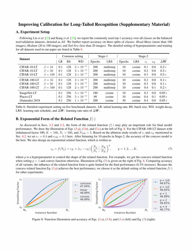
performance. We draw the illustration of Eqs. (3.a), (3.b), and (3.c) at the left of Fig. 8. For the CIFAR-100-LT dataset withimbalanced factor 100, K = 100, N1 = 500, and N100 = 5. Based on the ablation study results of ε1 and εK mentioned inSec. 4.2, we set ε1 = 0.4 and ε100 = 0.1 here. After fintuning for 10 epochs in Stage-2, the accuracy of the concave model isthe best. We also design an exponential related function, which is written as

εy = f(Ny) = εK + (ε1 − εK)

(Ny −NKN1 −NK

)p, y = 1, 2, ...,K, (7)

where p is a hyperparameter to control the shape of the related function. For example, we get the concave related functionwhen setting p < 1 and convex function otherwise. Illustration of Eq. (7) is given on the right of Fig. 8. Comparing accuracyof all variants, the influence of the related function form is quite limited for the final performance (0.3% increase). Because theconcave related function Eq. (3.a) achieves the best performance, we choose it as the default setting of the related function f(·)for other experiments.


K

1

Smoo

thin

g Fa

ctor concave

47.04%linear46.89%convex46.89%


K

1

Smoo

thin

g Fa

ctor

p = 1/446.67%p = 1/246.82%p = 146.89%p = 246.81%p = 446.77%

Figure 8: Function illustration and accuracy of Eqs. (3.a), (3.b), and (3.c) (left) and Eq. (7) (right).

C. Calibration Performance

Org. CIFAR-10 CIFAR10-LT, IF100 cRT LWS MiSLAS

0.0 0.2 0.4 0.6 0.8 1.0

0.2

0.4

0.6

0.8

1.0

Accu

racy

ACC=93.2%ECE=3.87%

GapAccuracy

0.0 0.2 0.4 0.6 0.8 1.0

ACC=72.3%ECE=20.1%

GapAccuracy

0.0 0.2 0.4 0.6 0.8 1.0

ACC=75.2%ECE=14.9%

GapAccuracy

0.0 0.2 0.4 0.6 0.8 1.0

ACC=74.0%ECE=19.6%

GapAccuracy

0.0 0.2 0.4 0.6 0.8 1.0

ACC=82.2%ECE=3.70%

GapAccuracy

Confidence

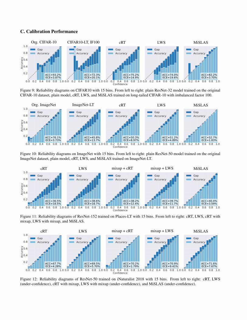
Figure 9: Reliability diagrams on CIFAR10 with 15 bins. From left to right: plain ResNet-32 model trained on the originalCIFAR-10 dataset, plain model, cRT, LWS, and MiSLAS trained on long-tailed CIFAR-10 with imbalanced factor 100.

Org. ImageNet ImageNet-LT cRT LWS MiSLAS

0.0 0.2 0.4 0.6 0.8 1.0

0.2

0.4

0.6

0.8

1.0

Accu

racy

ACC=76.1%ECE=3.73%

GapAccuracy

0.0 0.2 0.4 0.6 0.8 1.0

ACC=45.8%ECE=13.7%

GapAccuracy

0.0 0.2 0.4 0.6 0.8 1.0

ACC=50.3%ECE=8.97%

GapAccuracy

0.0 0.2 0.4 0.6 0.8 1.0

ACC=51.2%ECE=4.89%

GapAccuracy

0.0 0.2 0.4 0.6 0.8 1.0

ACC=52.7%ECE=1.83%

GapAccuracy

Confidence

Figure 10: Reliability diagrams on ImageNet with 15 bins. From left to right: plain ResNet-50 model trained on the originalImageNet dataset, plain model, cRT, LWS, and MiSLAS trained on ImageNet-LT.

cRT LWS mixup + cRT mixup + LWS MiSLAS

0.0 0.2 0.4 0.6 0.8 1.0

0.2

0.4

0.6

0.8

1.0

Accu

racy

ACC=36.5%ECE=18.5%

GapAccuracy

0.0 0.2 0.4 0.6 0.8 1.0

ACC=38.6%ECE=18.7%

GapAccuracy

0.0 0.2 0.4 0.6 0.8 1.0

ACC=38.2%ECE=12.4%

GapAccuracy

0.0 0.2 0.4 0.6 0.8 1.0

ACC=39.7%ECE=11.7%

GapAccuracy

0.0 0.2 0.4 0.6 0.8 1.0

ACC=40.4%ECE=3.59%

GapAccuracy

Confidence

Figure 11: Reliability diagrams of ResNet-152 trained on Places-LT with 15 bins. From left to right: cRT, LWS, cRT withmixup, LWS with mixup, and MiSLAS.

cRT LWS mixup + cRT mixup + LWS MiSLAS

0.0 0.2 0.4 0.6 0.8 1.0

0.2

0.4

0.6

0.8

1.0

Accu

racy

ACC=67.7%ECE=4.28%

GapAccuracy

0.0 0.2 0.4 0.6 0.8 1.0

ACC=69.5%ECE=5.70%

GapAccuracy

0.0 0.2 0.4 0.6 0.8 1.0

ACC=70.2%ECE=1.79%

GapAccuracy

0.0 0.2 0.4 0.6 0.8 1.0

ACC=70.9%ECE=9.41%

GapAccuracy

0.0 0.2 0.4 0.6 0.8 1.0

ACC=71.6%ECE=7.67%

GapAccuracy

Confidence

Figure 12: Reliability diagrams of ResNet-50 trained on iNaturalist 2018 with 15 bins. From left to right: cRT, LWS(under-confidence), cRT with mixup, LWS with mixup (under-confidence), and MiSLAS (under-confidence).

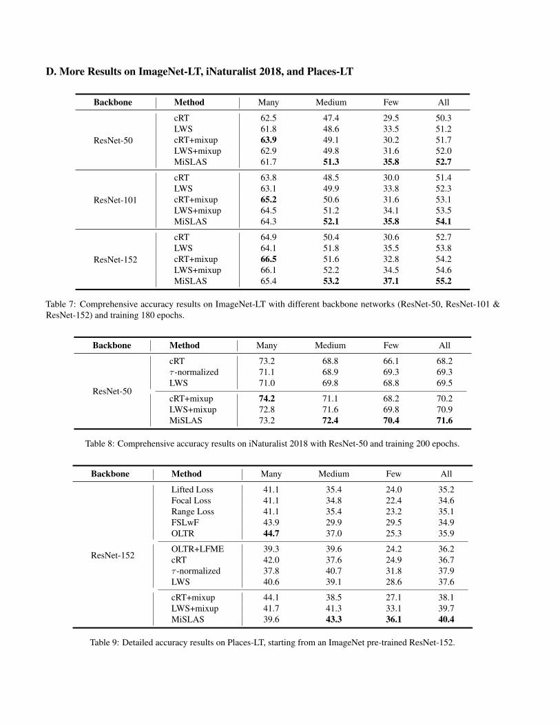
D. More Results on ImageNet-LT, iNaturalist 2018, and Places-LT

Backbone Method Many Medium Few All

ResNet-50

cRT 62.5 47.4 29.5 50.3LWS 61.8 48.6 33.5 51.2cRT+mixup 63.9 49.1 30.2 51.7LWS+mixup 62.9 49.8 31.6 52.0MiSLAS 61.7 51.3 35.8 52.7

ResNet-101


ResNet-152


Table 7: Comprehensive accuracy results on ImageNet-LT with different backbone networks (ResNet-50, ResNet-101 &ResNet-152) and training 180 epochs.


ResNet-50

cRT 73.2 68.8 66.1 68.2τ -normalized 71.1 68.9 69.3 69.3LWS 71.0 69.8 68.8 69.5

cRT+mixup 74.2 71.1 68.2 70.2LWS+mixup 72.8 71.6 69.8 70.9MiSLAS 73.2 72.4 70.4 71.6

Table 8: Comprehensive accuracy results on iNaturalist 2018 with ResNet-50 and training 200 epochs.


ResNet-152

Lifted Loss 41.1 35.4 24.0 35.2Focal Loss 41.1 34.8 22.4 34.6Range Loss 41.1 35.4 23.2 35.1FSLwF 43.9 29.9 29.5 34.9OLTR 44.7 37.0 25.3 35.9

OLTR+LFME 39.3 39.6 24.2 36.2cRT 42.0 37.6 24.9 36.7τ -normalized 37.8 40.7 31.8 37.9LWS 40.6 39.1 28.6 37.6

cRT+mixup 44.1 38.5 27.1 38.1LWS+mixup 41.7 41.3 33.1 39.7MiSLAS 39.6 43.3 36.1 40.4

Table 9: Detailed accuracy results on Places-LT, starting from an ImageNet pre-trained ResNet-152.

E. Proof of Eq. (2), the Optimal Solution of LASIn this section, we prove the optimal solutions of cross-entropy, the re-weighting method, and LAS. Furthermore, the

comparison among above three methods will also be discussed.The general loss function form of these three methods for K classes can be written as

l = −K∑i=1

qi log pi, pi = softmax(w>i x), s.t.,

K∑i

pi = 1, (8)

where p,w, and x are the predicted probability, the weight parameter of the last fully-connected layer, and the input of the lastfully-connected layer, respectively. When the target label q is defined as

qi =

{1, i = y,0, i 6= y,

where y is the original ground truth label. Eq. (8) becomes the commonly used cross-entropy loss function. Similarly, whenthe target label q is defined as

qi =

{wi, i = y, and wi > 0,0, i 6= y,

Eq. (8) becomes the re-weighting loss function. Moreover, when the target label q is

qi =

{1− εy = 1− f(Ny), i = y,εyK−1 =

f(Ny)K−1 , i 6= y,

(9)

Eq. (8) becomes the proposed LAS method. To get the optimal solution of Eq. (8), we define its Lagrange multiplier form as

L = l + λ

(K∑i

pi − 1

)= −

K∑i=1

qi log pi + λ

(K∑i

pi − 1

), (10)

where λ is the Lagrange multiplier. The first order conditions of Eq. (10) w.r.t. λ and p can be written as

∂L

∂λ=

K∑i=1

pi − 1 = 0,

∂L

∂pi= −qi

pi+ λ = 0.

(11)

According to Eq. (11), we get pi = qi∑Kj=1 qj

. Then, in the case of cross-entropy and re-weighting loss function, we get

pi = 1, i = y and pi = 0, i 6= y. Noting that

pi = softmax(w>i x) =exp(w>i x)∑Kj=1 exp(w>j x)

,

the optimal solutions of w>i x for both cross-entropy and re-weighting loss functions are the same, that is, w∗i>x = inf .

This means that both cross-entropy and re-weighting loss functions make the weight vector of the right class wi, i = y largeenough while the others wj , j 6= y sufficiently small. As a result, they cannot change the predicted distribution and relieveover-confidence effectively. In contrast, in our LAS, according to Eqs. (9) and (11), we get

pi =exp(w>i x)∑Kj=1 exp(w>j x)

=qi∑Kj=1 qj

=

{1− εy, i = y,εyK−1 , i 6= y,

=⇒ w∗i>x =

{log[(K−1)(1−εy)

εy

]+ c, i = y,

c, i 6= y,(12)

where c ∈ R can be an arbitrary real number. Overall, comparing with the infinite optimal solution in cross-entropy andre-weighting method, LAS encourages a finite output, which leads to a more general result, properly refines the predicteddistributions of the head, medium, and tailed classes, and remedies over-confidence effectively.

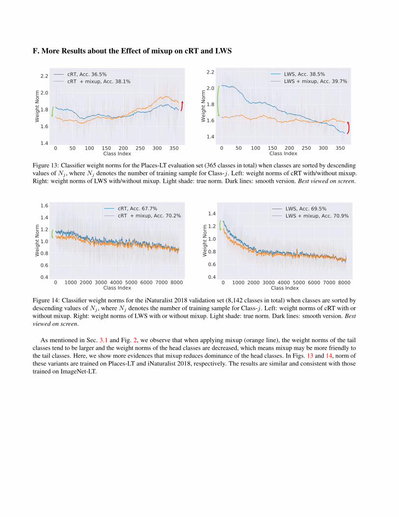
F. More Results about the Effect of mixup on cRT and LWS

Figure 13: Classifier weight norms for the Places-LT evaluation set (365 classes in total) when classes are sorted by descendingvalues of Nj , where Nj denotes the number of training sample for Class-j. Left: weight norms of cRT with/without mixup.Right: weight norms of LWS with/without mixup. Light shade: true norm. Dark lines: smooth version. Best viewed on screen.

Figure 14: Classifier weight norms for the iNaturalist 2018 validation set (8,142 classes in total) when classes are sorted bydescending values of Nj , where Nj denotes the number of training sample for Class-j. Left: weight norms of cRT with orwithout mixup. Right: weight norms of LWS with or without mixup. Light shade: true norm. Dark lines: smooth version. Bestviewed on screen.

As mentioned in Sec. 3.1 and Fig. 2, we observe that when applying mixup (orange line), the weight norms of the tailclasses tend to be larger and the weight norms of the head classes are decreased, which means mixup may be more friendly tothe tail classes. Here, we show more evidences that mixup reduces dominance of the head classes. In Figs. 13 and 14, norm ofthese variants are trained on Places-LT and iNaturalist 2018, respectively. The results are similar and consistent with thosetrained on ImageNet-LT.

Documents

Improving Calibration for Long-Tailed Recognition