Embed Size (px)
Citation preview
Improving climate projections using “intelligent” ensembles
Noël C. Baker and Patrick C. Taylor
NASA Postdoctoral Program
Presented at the AGU Joint Assembly in Montréal, Canada
May 5, 2015
Langley
Research
Center
2
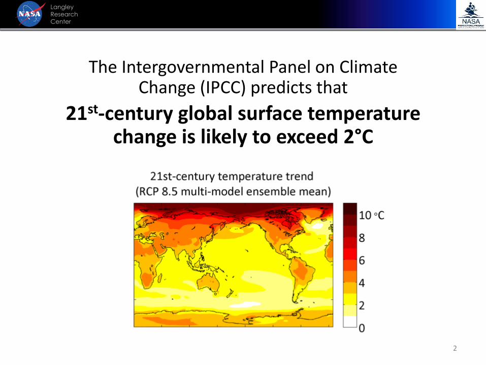
The Intergovernmental Panel on Climate Change (IPCC) predicts that
21st-century global surface temperature change is likely to exceed 2°C
Langley
Research
Center
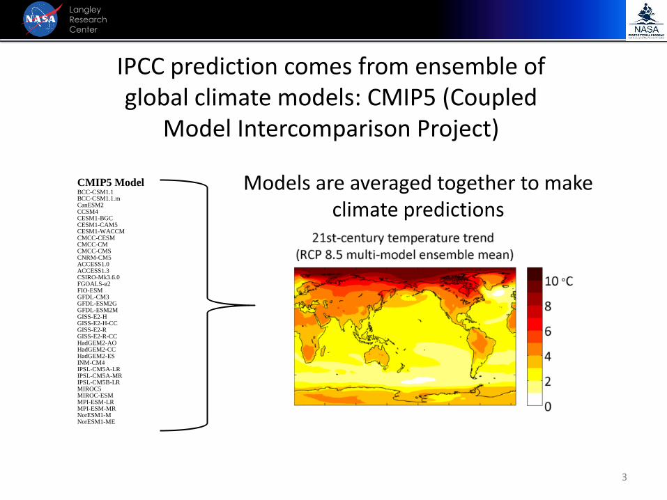
CMIP5 Model BCC-CSM1.1 BCC-CSM1.1.m CanESM2 CCSM4 CESM1-BGC CESM1-CAM5 CESM1-WACCM CMCC-CESM CMCC-CM CMCC-CMS CNRM-CM5 ACCESS1.0 ACCESS1.3 CSIRO-Mk3.6.0 FGOALS-g2 FIO-ESM GFDL-CM3 GFDL-ESM2G GFDL-ESM2M GISS-E2-H GISS-E2-H-CC GISS-E2-R GISS-E2-R-CC HadGEM2-AO HadGEM2-CC HadGEM2-ES INM-CM4 IPSL-CM5A-LR IPSL-CM5A-MR IPSL-CM5B-LR MIROC5 MIROC-ESM MPI-ESM-LR MPI-ESM-MR NorESM1-M NorESM1-ME
3
Models are averaged together to make climate predictions
IPCC prediction comes from ensemble of global climate models: CMIP5 (Coupled
Model Intercomparison Project)
Langley
Research
Center
4
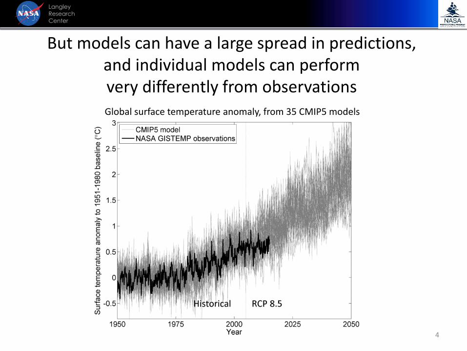
But models can have a large spread in predictions, and individual models can perform very differently from observations
Langley
Research
Center
Global surface temperature anomaly, from 35 CMIP5 models
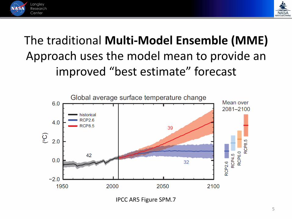
The traditional Multi-Model Ensemble (MME) Approach uses the model mean to provide an
improved “best estimate” forecast
5
Langley
Research
Center
IPCC AR5 Figure SPM.7
6
Langley
Research
Center
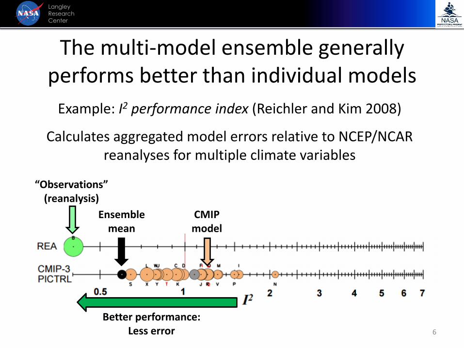
The multi-model ensemble generally performs better than individual models
Example: I2 performance index (Reichler and Kim 2008)
Calculates aggregated model errors relative to NCEP/NCAR reanalyses for multiple climate variables
Ensemble mean
“Observations” (reanalysis)
CMIP model
Better performance:Less error
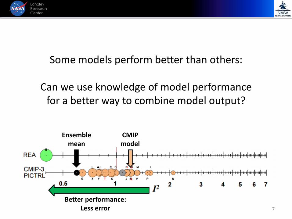
Some models perform better than others:
Can we use knowledge of model performance for a better way to combine model output?
7
Langley
Research
Center
Ensemble mean
CMIP model
Better performance:Less error
8
Langley
Research
Center
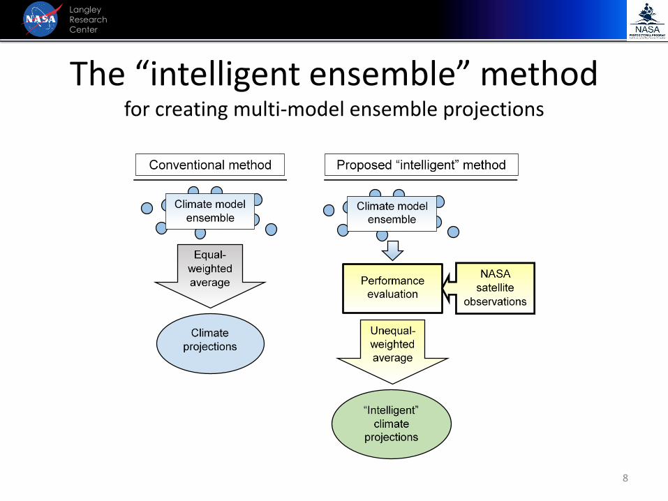
The “intelligent ensemble” methodfor creating multi-model ensemble projections
9
Langley
Research
Center
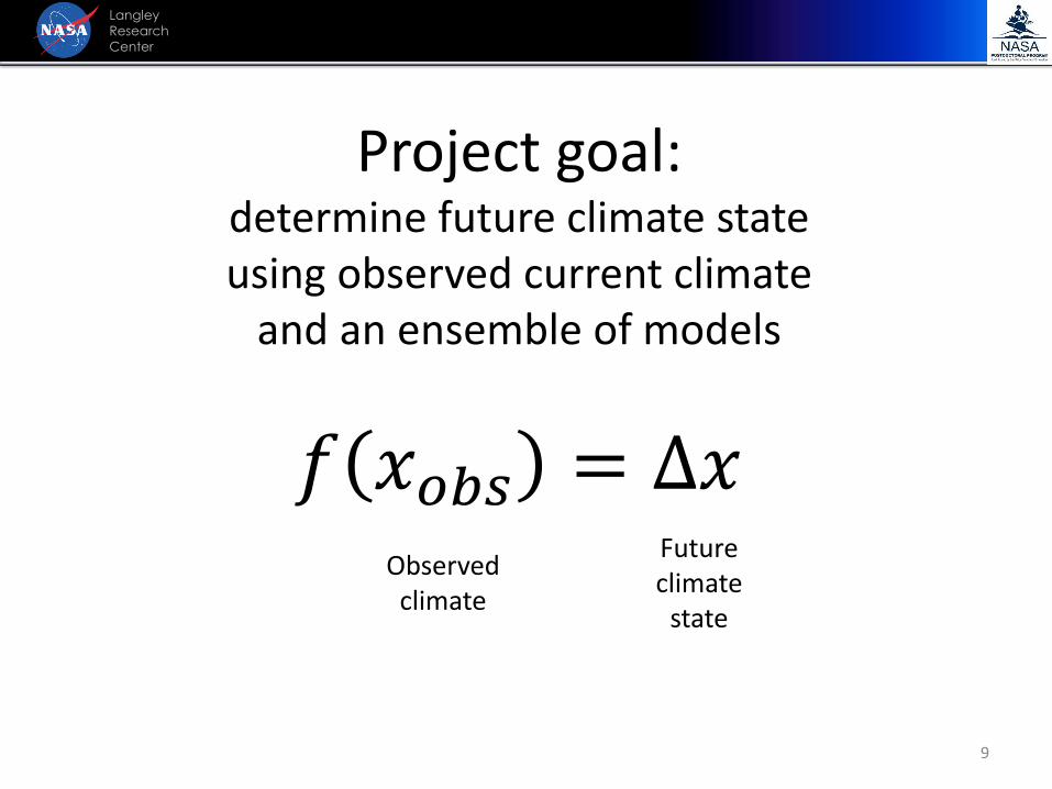
Project goal:determine future climate state using observed current climate
and an ensemble of models
𝑓 𝑥𝑜𝑏𝑠 = Δ𝑥Future climate
state
Observed climate
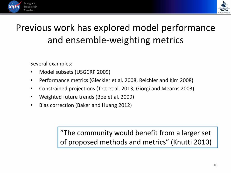
Several examples:
• Model subsets (USGCRP 2009)
• Performance metrics (Gleckler et al. 2008, Reichler and Kim 2008)
• Constrained projections (Tett et al. 2013; Giorgi and Mearns 2003)
• Weighted future trends (Boe et al. 2009)
• Bias correction (Baker and Huang 2012)
10
“The community would benefit from a larger set of proposed methods and metrics” (Knutti 2010)
Previous work has explored model performance and ensemble-weighting metrics
Langley
Research
Center
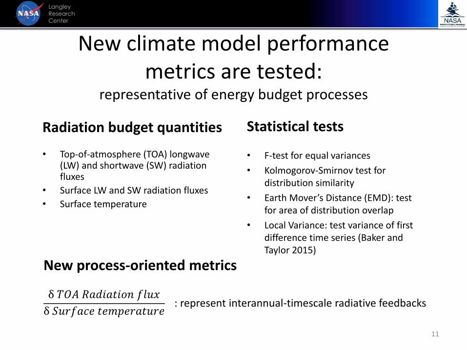
New climate model performance metrics are tested:
representative of energy budget processes
11
Langley
Research
Center
Radiation budget quantities
• Top-of-atmosphere (TOA) longwave(LW) and shortwave (SW) radiation fluxes
• Surface LW and SW radiation fluxes
• Surface temperature
Statistical tests
• F-test for equal variances
• Kolmogorov-Smirnov test for distribution similarity
• Earth Mover’s Distance (EMD): test for area of distribution overlap
• Local Variance: test variance of first difference time series (Baker and Taylor 2015)
New process-oriented metrics
δ 𝑇𝑂𝐴 𝑅𝑎𝑑𝑖𝑎𝑡𝑖𝑜𝑛 𝑓𝑙𝑢𝑥
δ 𝑆𝑢𝑟𝑓𝑎𝑐𝑒 𝑡𝑒𝑚𝑝𝑒𝑟𝑎𝑡𝑢𝑟𝑒: represent interannual-timescale radiative feedbacks
12
Langley
Research
Center
Model data: 32 CMIP5 models http://pcmdi9.llnl.gov/
• ‘Pre-Industrial Control’ simulations (monthly mean, 100 years) to create metric weights
• ‘RCP 8.5’ future simulations (monthly mean, 2081-2100 minus 2011-2030 to produce 21st-century trends)
Observational datasets:
NASA CERES EBAF-TOA and surface monthly global-mean (full data record: 03/2000 - 05/2014)http://ceres.larc.nasa.gov/
NASA GISS Surface Temperature Analysis (GISTEMP)http://data.giss.nasa.gov/gistemp/
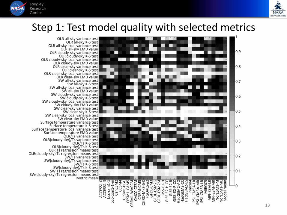
Step 1: Test model quality with selected metrics
13
Langley
Research
Center
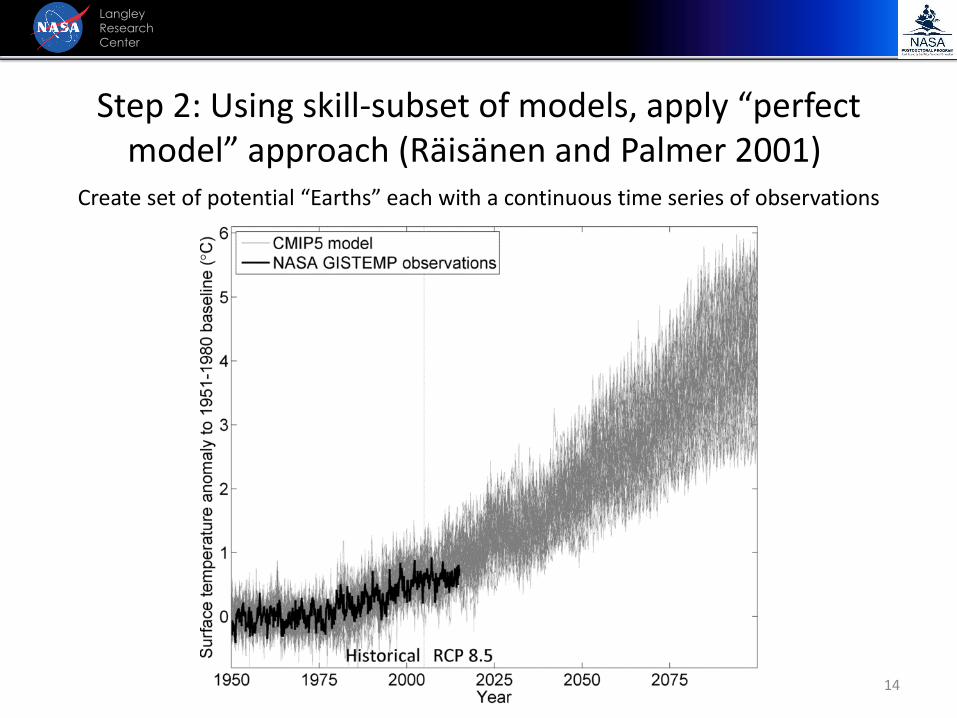
Step 2: Using skill-subset of models, apply “perfect model” approach (Räisänen and Palmer 2001)
Create set of potential “Earths” each with a continuous time series of observations
14
Langley
Research
Center
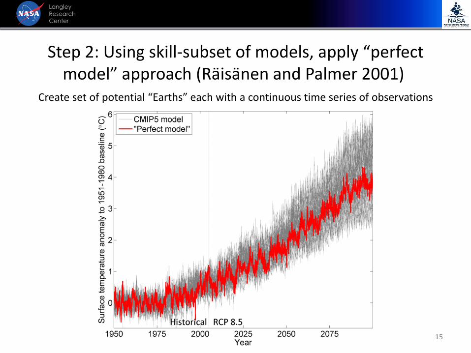
Step 2: Using skill-subset of models, apply “perfect model” approach (Räisänen and Palmer 2001)
Create set of potential “Earths” each with a continuous time series of observations
15
Langley
Research
Center
16
Langley
Research
Center
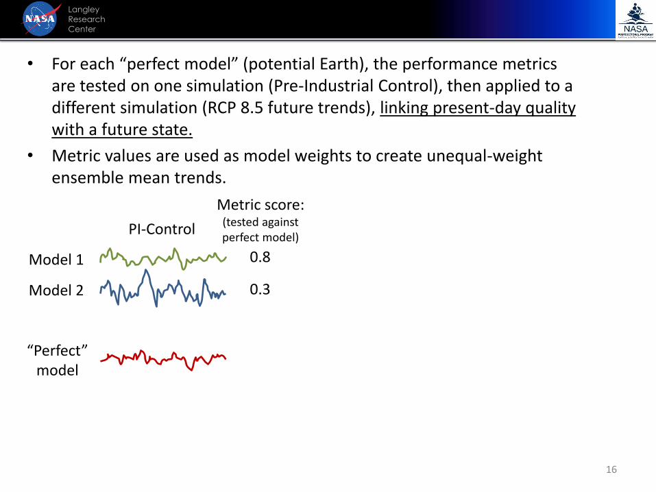
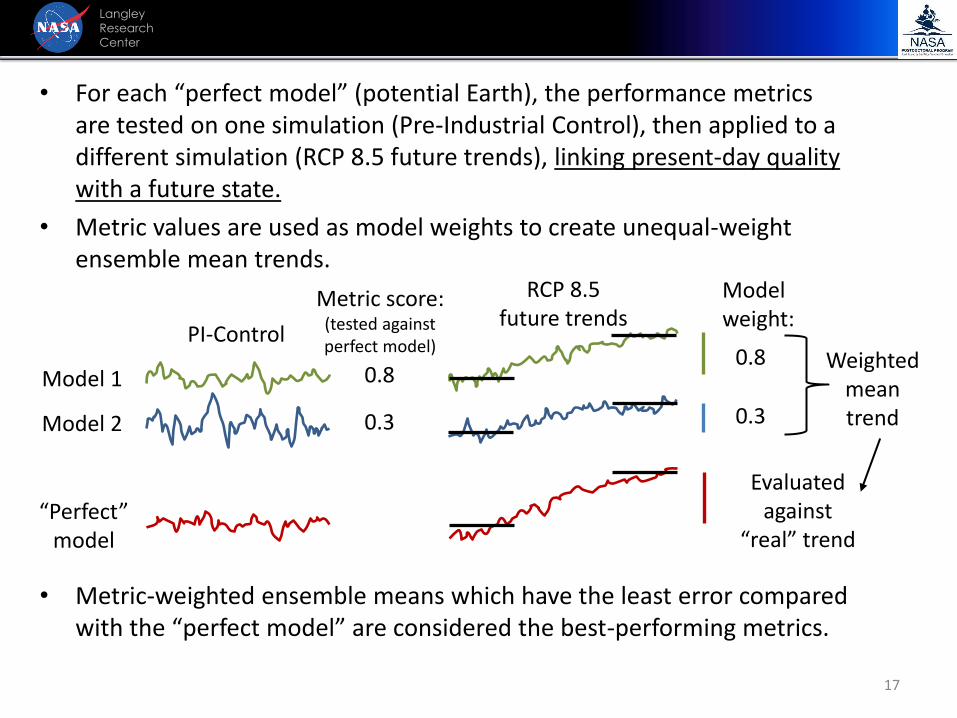
• For each “perfect model” (potential Earth), the performance metrics are tested on one simulation (Pre-Industrial Control), then applied to a different simulation (RCP 8.5 future trends), linking present-day quality with a future state.
• Metric values are used as model weights to create unequal-weight ensemble mean trends.
Model 1
Model 2
“Perfect” model
Metric score: (tested against perfect model)
0.8
0.3
PI-Control
17
Langley
Research
Center
• For each “perfect model” (potential Earth), the performance metrics are tested on one simulation (Pre-Industrial Control), then applied to a different simulation (RCP 8.5 future trends), linking present-day quality with a future state.
• Metric values are used as model weights to create unequal-weight ensemble mean trends.
• Metric-weighted ensemble means which have the least error compared with the “perfect model” are considered the best-performing metrics.
Model 1
Model 2
“Perfect” model
Metric score: (tested against perfect model)
0.8
0.3
PI-Control
RCP 8.5 future trends
Model weight:
0.8
0.3
Weighted mean trend
Evaluated against
“real” trend
18
Langley
Research
Center
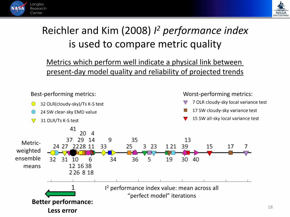
I2 performance index value: mean across all “perfect model” iterations
Metric-weighted ensemble
means
Better performance:Less error
Reichler and Kim (2008) I2 performance index is used to compare metric quality
Best-performing metrics: Worst-performing metrics:
Metrics which perform well indicate a physical link between present-day model quality and reliability of projected trends
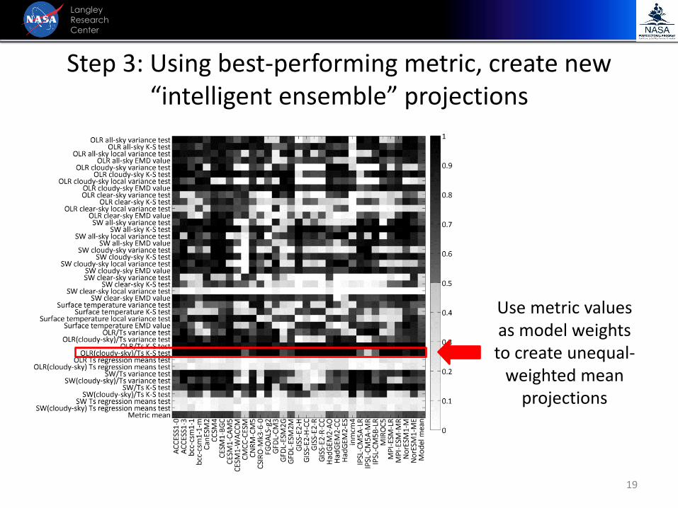
Step 3: Using best-performing metric, create new “intelligent ensemble” projections
19
Langley
Research
Center
Use metric values as model weights to create unequal-
weighted mean projections
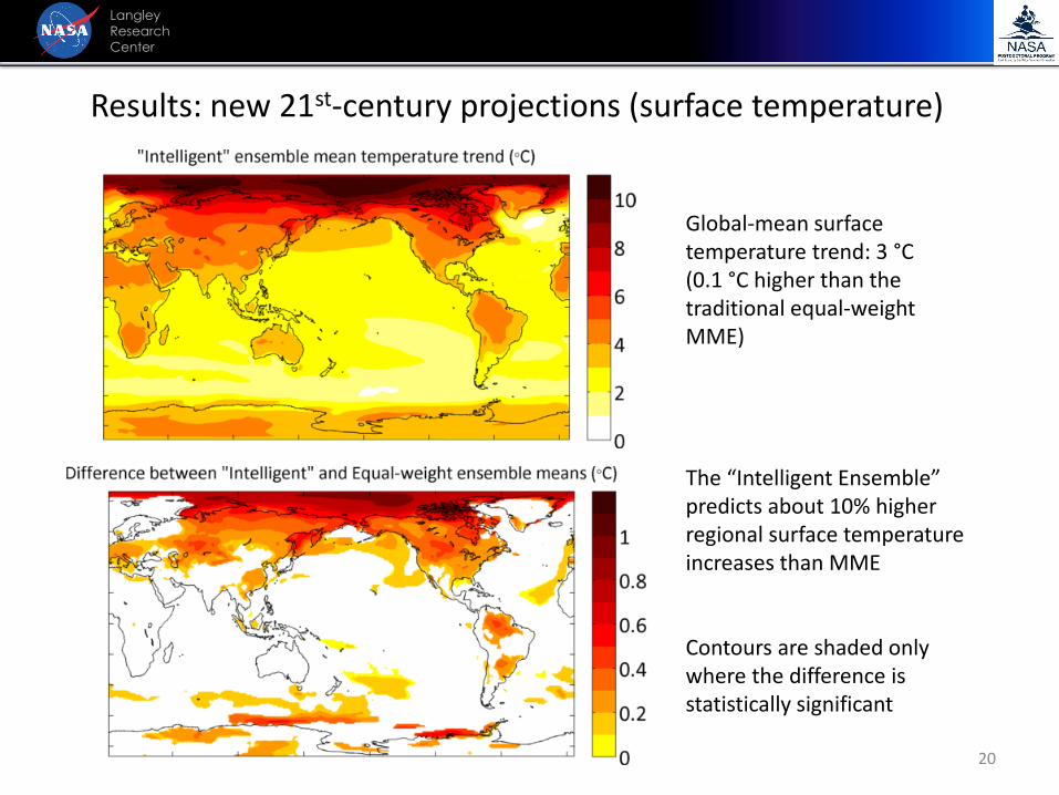
Results: new 21st-century projections (surface temperature)
20
Langley
Research
Center
Global-mean surface temperature trend: 3 °C(0.1 °C higher than the traditional equal-weight MME)
The “Intelligent Ensemble” predicts about 10% higher regional surface temperature increases than MME
Contours are shaded only where the difference is statistically significant
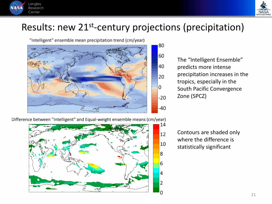
Results: new 21st-century projections (precipitation)
21
Langley
Research
Center
The “Intelligent Ensemble” predicts more intense precipitation increases in the tropics, especially in the South Pacific Convergence Zone (SPCZ)
Contours are shaded only where the difference is statistically significant
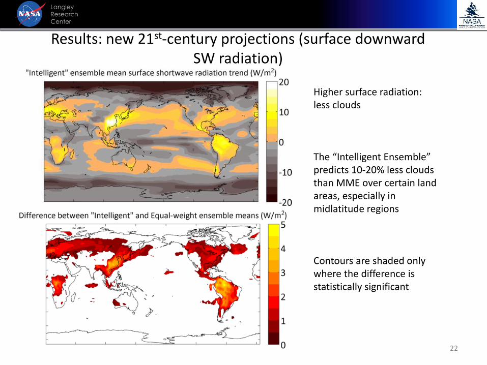
Results: new 21st-century projections (surface downward SW radiation)
22
Langley
Research
Center
Higher surface radiation: less clouds
The “Intelligent Ensemble” predicts 10-20% less clouds than MME over certain land areas, especially in midlatitude regions
Contours are shaded only where the difference is statistically significant
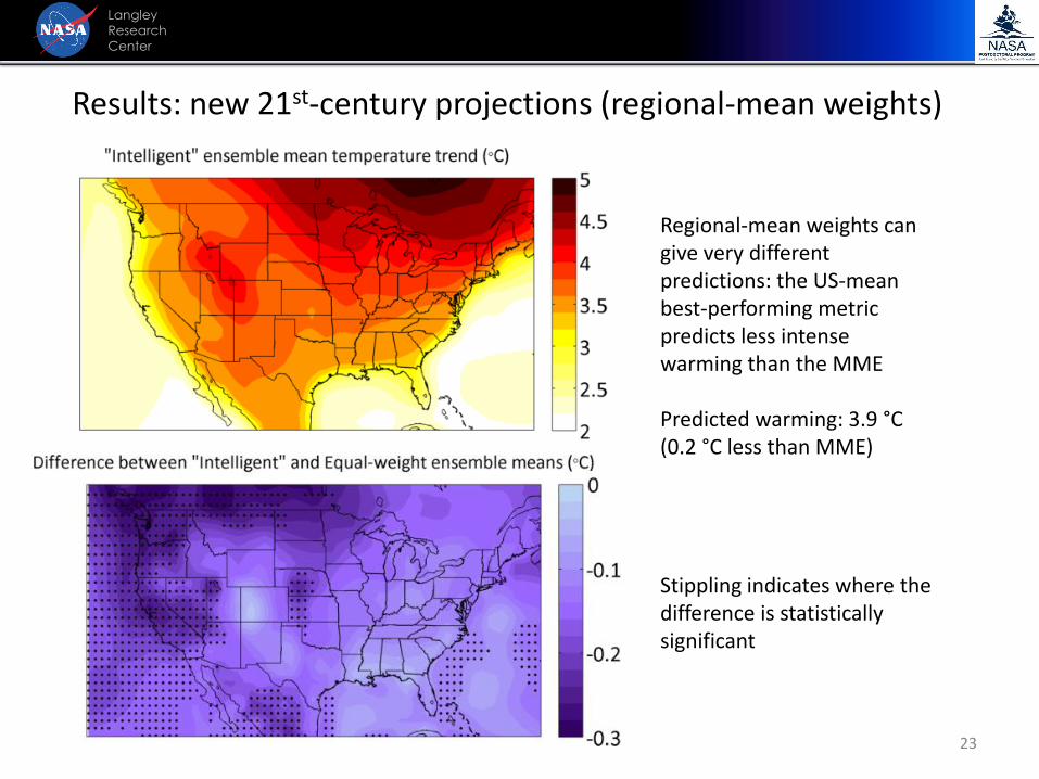
Results: new 21st-century projections (regional-mean weights)
23
Langley
Research
Center
Regional-mean weights can give very different predictions: the US-mean best-performing metric predicts less intense warming than the MME
Predicted warming: 3.9 °C(0.2 °C less than MME)
Stippling indicates where the difference is statistically significant
24
Langley
Research
Center
Conclusions
This project demonstrates:• New climate model performance metrics related to radiation
processes are tested on the CMIP5 archive• Present-day model skill is linked to quality of future projections
The results are:• New “intelligent ensemble” projections are created and compared
with traditional MME projections• For global-mean metrics, “intelligent ensemble” projections of
large-scale patterns remain similar, but intensity of predicted surface temperature, precipitation, and surface radiation increase is 10-20% higher than the MME
• Regional-mean metrics can produce very different projections: the US-mean projected warming is 3.9 °C (0.2 °C less than MME)