IMPROVING CONVERGENCE TIME OF THE ELEC- … · IMPROVING CONVERGENCE TIME OF THE ELEC-TROMAGNETIC INVERSE METHOD BASED ... based on a network of electric and magnetic ... adaptive

Progress In Electromagnetics Research B, Vol. 51, 389–406, 2013

IMPROVING CONVERGENCE TIME OF THE ELEC-TROMAGNETIC INVERSE METHOD BASED ON GE-NETIC ALGORITHM USING THE PZMI AND NEURALNETWORK

Sofiene Saidi* and Jaleleddine Ben Hadj Slama

SAGE, National Engineering School of Sousse, (ENISo), University ofSousse, Technopole of Sousse, Sousse 4054, Tunisia

Abstract—In this paper we present a methodology to guarantee theconvergence of the electromagnetic inverse method. This method isapplied to electromagnetic compatibility (EMC) in order to overcomethe difficulties of measuring the radiated electromagnetic field and toreduce the cost of the EMC analysis. It consists in using GeneticAlgorithms (GA) to identify a model that will be used to estimate theelectric and magnetic field radiated by the device under test. Thismethod is based on the recognition of the equivalent radiation sourcesusing the Near Field (NF) cartography radiated by the device. Ourcontribution in this field is to improve the ability and the convergenceof the electromagnetic inverse method by using the Pseudo ZernikeMoment Invariant (PZMI) descriptor and the Artificial Neural Network(ANN). The validation of the proposed method is performed using theNF emitted by known electric and magnetic dipoles. Our results haveproved that the proposed method guarantees the convergence of theelectromagnetic inverse method and that the convergence speeds upwhile retaining all the other performances.

1. INTRODUCTION

The rapid development of electrical systems has created the need toanalyze and control their electromagnetic radiation. Therefore, theknowledge of the electromagnetic field distribution of any electricaldevice is necessary. Since the electrical device is composed by complexand active components, the computation of the Near Field (NF) andFar Field (FF) has many difficulties. A new technique, called the NearField (NF) technique, has been developed to overcome this problem.

Received 16 September 2012, Accepted 29 April 2013, Scheduled 15 May 2013* Corresponding author: Sofiene Saidi ([email protected]).

390 Saidi and Ben Hadj Slama

The measurement of the electromagnetic NF is made with agood signal-to-noise ratio (S/N) because it is taken in a region veryclose to the radiation source. Thus, it does not require a particularmeasurement environment such as those required when measuringthe electromagnetic FF (anechoic chamber). In addition, the NFcartography is directly related to the device geometry (the positions ofradiation sources).

The electromagnetic inverse method is based on the NFtechnique [1, 2]. A model of a microcontroller has been described byelectric dipoles using measurements of the magnetic NF componentsHx and Hy. This model was created by inverting the matrix and itcan calculate only the magnetic field [3]. This model was improved bycoupling the digital image processing technique with the optimizationalgorithm [4]. In order to predict the magnetic and electric NF, [5, 6]developed a model based on a network of electric and magnetic dipoles.

The resolution with the inverse electromagnetic method requiresan optimization method such as the Genetic Algorithms (GA) [7].In [8] an adaptive GA was applied to model a DC-DC converter.[9] used a binary GA optimization method to simulate wire andresonator antennas. Another study [10] considered that loops werethe mainly radiation sources in circuits and used the GA to identifythe rectangular loops in the circuit.

The study [11] shows that the optimization method based on GAis the most powerful in terms of accuracy compared to that based onthe Fast Fourier Transform (FFT) or on an integral equation.

The convergence of the electromagnetic inverse method basedon the GA requires a significant calculation time. The GA methodis characterized by several parameters. A judicious choice of theseparameters can accelerate the convergence of this method. In aprevious work [12], we explored some parameters that can influencethe efficiency of the convergence of the electromagnetic inverse methodbased on the GA. These parameters are: the population size, thecrossover rate, the selection function, and the fitness function. So,a judicious choice of these parameters can accelerate the convergenceof the electromagnetic inverse method to the final solution in a shortertime. In order to adapt this method to the electronic power system, [7]coupled the electromagnetic inverse method with a numerical method:the Moments Method (MoM). This new approach demonstrates theability of this coupling in modeling the radiation of large circuits suchas those used in power electronic systems.

In this work, we propose to improve the electromagnetic inversemethod based on the GA. Our contribution consists in coupling thelatter method with a powerful technique. This technique, called the

Progress In Electromagnetics Research B, Vol. 51, 2013 391

Pseudo Zernike Moment Invariant (PZMI), has been used in the recentyears in the digital image processing and faces recognition,thanks toits superior future representation capability [13]. The PZMI vectoris applied, in our case, to represent the radiated NF as a complexvector. The proposed methodology has coupled different methodsused in the literature: image processing, the GA and the NeuralNetwork (NN). It has at least three main advantages when comparingit to other approaches [3]: firstly, it guarantees the convergence ofthe electromagnetic inverse method and it speeds up the convergence;secondly, it makes the source identification using the magnitude of onlyone component of the magnetic field (Hz); and finally, it works even ifall the dipoles parameters are not known.

In this paper, we will describe the electromagnetic inverse methodbased on the GA in Section 2. In Section 3, we will introduce theproposed approach. Consequently, we will explain the choice of theused scan-window as well as the application of the PZMI descriptorwith the Neural Network to classify the radiation sources. In Section4, we will describe the implementation of the proposed method andthe obtained results when using an NF cartography radiated by animportant number of dipoles. In order to examine the ability ofour contribution we will compare results to those obtained using theclassical method. Finally, we will focus on the robustness of theproposed method.

2. THE ELECTROMAGNETIC INVERSE METHODBASED ON GENETIC ALGORITHMS

The electromagnetic inverse method consists in using NF measure-ments to modelize the studied system by a network of electric or mag-netic dipoles or both of them. The modeling procedure is resumed inthree steps (Figure 1). First, the NF measurements are made at anh height which is very low compared to λ

2π ( λ2π is the limit between

the NF and the FF, where λ is the wavelength). Therefore, the NFpresented as a cartography, which allows us to locate the regions of thehigh or low electromagnetic field radiated by an electronic board. Inthis study, we have chosen the vertical component of the magnetic fieldHz. However we can apply the method with the other magnetic fieldcomponents Hx and Hy. In a second step, using the measured NF, theGA proceeds to seek for optimum parameters of the dipoles (magneticmoments, positions and orientations) that will give a calculated fieldwhich is closer to the measured NF. In a third step, the identified pa-rameters are used to estimate the electromagnetic field emitted at anypoint in the space. The optimization fitness function (1) that we have


Measured

NF

Simulated and measured

NF and FF

Direct method

Device Under TestGA search the

parameters of dipoles

Using the model to calculate the NF and FF at any distance

1

2

3

Figure 1. The electromagnetic inverse method based on the GA.

used to provide a comparison between the measured and the estimatedNF is the Euclidean distance between the two cartographies.

F =∑

|NFmeasured −NF calculated| (1)

Also, to overcome problems related to measurement errorswhen doing validations, we have applied in this work the proposedmethodology only to the cartographies of the calculated NF values.

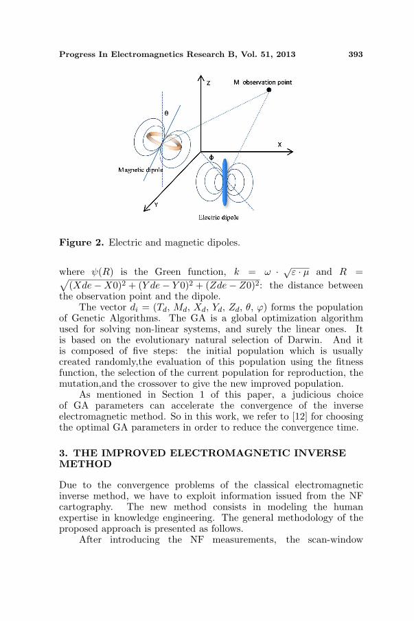
An elementary magnetic or electric radiating dipole (Figure 2)is characterized by a set of parameters. That is why a dipole canbe represented by a di vector which includes all the parametersdi = (Td, Md, Xd, Yd, Zd, θ, ϕ), where Td is the type of dipole, Md

is the magnetic moment, (Xd, Yd, Zd) is the dipole position and θ, ϕis the dipole orientation.

The magnetic field Hz radiated by the two elementary dipoles isdescribed with the analytical Equations (2) and (3).

For the electric dipole:

HZ =j ·k ·Md

4 · π ·R ·ψ(R)·(1+

1j ·k ·R

)·(

sin (θ) sin (ϕ) · (Y de−Y 0)− sin (θ) cos (ϕ) · (Xde−X0)

)(2)

and for the magnetic dipole:

HZ =−k2

4ψ(R)·Md ·

((1+ 1

j·k·R + 1(j·k·R)2

)· cos(θ)

)

−

(1+ 3

j·k·R + 3(j·k·R)2

)· 1R2 ·(Zde−Z0)

·( cos(θ)(Zde− Z0)

+ sin(θ) cos(ϕ)(Y de− Y 0)+ sin(θ) sin(ϕ) · (Xde−X0)

)

(3)


Figure 2. Electric and magnetic dipoles.

where ψ(R) is the Green function, k = ω · √ε · µ and R =√(Xde−X0)2 + (Y de− Y 0)2 + (Zde− Z0)2: the distance between

the observation point and the dipole.The vector di = (Td, Md, Xd, Yd, Zd, θ, ϕ) forms the population

of Genetic Algorithms. The GA is a global optimization algorithmused for solving non-linear systems, and surely the linear ones. Itis based on the evolutionary natural selection of Darwin. And itis composed of five steps: the initial population which is usuallycreated randomly,the evaluation of this population using the fitnessfunction, the selection of the current population for reproduction, themutation,and the crossover to give the new improved population.

As mentioned in Section 1 of this paper, a judicious choiceof GA parameters can accelerate the convergence of the inverseelectromagnetic method. So in this work, we refer to [12] for choosingthe optimal GA parameters in order to reduce the convergence time.

3. THE IMPROVED ELECTROMAGNETIC INVERSEMETHOD

Due to the convergence problems of the classical electromagneticinverse method, we have to exploit information issued from the NFcartography. The new method consists in modeling the humanexpertise in knowledge engineering. The general methodology of theproposed approach is presented as follows.

After introducing the NF measurements, the scan-window


algorithm extracts a local NF cartography using an appropriatewindow. Then the scan-window algorithm moves up the window untilidentifying two dipole parameters: the type (electric or magnetic) andthe position (Xd, Yd) [14]. The other parameters (magnetic momentMd and the orientation θ and ϕ) will be identified by the GA.

The obtained dipole parameters are then used to calculate valuesof the radiated NF from the dipole. The calculated values aresubtracted from the initial cartography. The above procedure isrepeated until extracting and identifying of all the radiating sources(Figure 3).

d

The measured NF The scan window Detected dipoleH (A/m)z

90807060

50

40

3020

100

90807060

5040

3020

100

908070

60

50

40

3020

10

090807060504030201009080706050403020100

9080706050403020100

0.90.80.7

0.6

0.5

0.4

0.3

0.20.1

0.90.80.7

0.6

0.5

0.4

0.3

0.20.1

0.90.80.7

0.6

0.5

0.4

0.3

0.20.1

Calculated the NF radiated by the

dipole and substracted from the

initial cartography

using GA

Identify (M , θ, ϕ)

Figure 3. The improved electromagnetic inverse method.

The proposed method consists in using the GA as a subprogramto find three parameters (Md, θ and ϕ) of one dipole whose positionand type are identified with the scan-window algorithm. The latter isbased on two algorithms: the PZMI descriptors and the NN.

3.1. The Scan-window Algorithm

The studied cartography is represented by a matrix containingmeasured amplitudes of the vertical component of the magnetic field.The cartography dimension usually depends on measuring parameterssuch as the size of the scan area, the distance between the probe andthe studied system and the step between two acquisition points alonghorizontal directions. This cartography contains information about thedistribution and amplitude of the electromagnetic NF radiated by theDevice Under Test (DUT).

In order to achieve the purpose of our study, which consists inusing the NF cartography to detect and identify the radiating sources,we propose to use the diagram given in Figure 4.


x

y

NF cartography

Compute the PZMI

vector

Classify dipoles

using the ANN

PZ

MI

Figure 4. The scan-window algorithm.

In order to properly proceed with the NF cartography, we chooserecent techniques used in the pattern of fingerprint recognition andidentification: the PZMI descriptors and the Neural Network (NN).These techniques are based on extracting the vector characteristicsof an image. This step consists in assimilating all the essential andrelevant information of an image as a low dimensional moment vector.The main aim of this project is to reduce the amount of parameters tobe determined by the GA. For this reason, we have decided to use thePZMI method.

3.2. The Scan-window Choice

The objective of this section is to justify the choice of the scan-window. Firstly, we define a suitable window on which we scan the

10 cm

x

y

2 mm measurement resolution

Scan-window (2×2 cm)

10 cm

2 cm

2 cm

2 mm

2 m

m

Figure 5. The scan-window.


NF cartography and then we use the scanned cartography to search alocal dipole. The study [14] shows that the choice of the scan windowdepends on the measured cartography size, resolution and height. Wesuppose that in our scan window, we have only one dipole at maximum.To overcome the limitations of this hypothesis, we can extend thelearning base with additional cases such as two or more dipoles atthe same scan-window.

[13] approved, by using several cartographies for variousconfigurations, that the ability of the method based on the PZMI wouldincrease with the number of measurement points. Referring to [14],we have selected the optimal size of the scan-window. Consequently,we have chosen the measured cartography equal to 10 × 10 cm at anh = 2 cm height and with a measurement resolution equal to 2mm(Figure 5).

3.3. Pseudo-Zernike Moment Invariant

The Zernike moments are orthogonal complex moments that candescribe an image by a complex vector. The amplitude of this vectoris characterized byan invariance when rotating [15, 16].

In this method, the area is set by orthogonal pseudo-Zernikepolynomials, defined as polar coordinates inside the unit circle. Thetwo-dimensional pseudo-Zernike moment Znm, for an order n and arepetition m, is defined using an image intensity function f(ρ, θ) asgiven in Equations (4), (5) and (6).

Znm =n + 1

π

∑x

∑y

f (x, y) V ∗nm (x, y) , x2 + y2 ≤ 1 (4)

Vnm = Rnm(ρ)e−jmθ (5)

where ρ =√

x2 + y2, θ = tan−1(xy ).

Rnm(ρ) =

n−|m|2∑

s=0

(−1)s (n− s)!

s!(

n+|m|2 − s

)!(

n−|m|2 − s

)!ρn−2s (6)

Table 1. PZMI vector of order 4.

Rnm n = 0 n = 1 n = 2 n = 3

m = 0 1 −2 + 3ρ 3 + 10ρ2 − 12ρ −4 + 35ρ3 − 60ρ2 + 30ρ

m = 1 0 ρ 5ρ2 − 4ρ 21ρ3 − 302 + 10ρ

m = 2 0 0 ρ2 7ρ3 − 6ρ2

m = 3 0 0 0 ρ3


where Znm is the moment of Zernike, Vnm the function of Zernike, andRnm the radial polynomial of Zernike.

Using the previous equations, we calculate the PZMI vector oforder 4 as described in (Table 1).

The PZMI vector of order 4 for the NF cartography has 9 complexnumbers that describe amplitudes and phases. To evaluate the rotationinvariance of the descriptor PZMI, we calculate the PZMI vector of themagnetic field radiated by a magnetic dipole for several orientations.First, in Figure 6, we give the cartographies of the z-component of themagnetic field radiated by a magnetic dipole for several orientations.

20 40 60 80 100 120 140 160

180 200 20 40 60 80 100 120 140 160 180 200 20 40 60 80 100 120 140 160 180 200

20 40 60 80 100 120 140 160 180 200 20 40 60 80 100 120 140 160 180 200

20

40

60

80

100

120

140

160

180

200

20

40

60

80

100

120

140

160

180

200

20

40

60

80

100

120

140

160

180

200

20

40

60

80

100

120

140

160

180

200

20

40

60

80

100

120

140

160

180

200

Φ = 0 Φ = 30 Φ = 45

Φ = 90 Φ = 135

O O O

O O

Figure 6. The cartographies of the z-component of the magnetic fieldradiated by a magnetic dipole for several orientations.

Afterwards, we determine the PZMI vector for all the NFcartographies. Table 2 represents only the amplitude of the PZMIvectors and the invariance rate σ(%).

The image of a cartography radiated by a dipole is easier toidentify then that of a face. So, the identification of dipoles usingcartography is not as complicated as the face recognition. The studyof the PZMI vector invariance shows that with a moment order equalto 4, the PZMI can describe a dipole for different orientations withan accuracy equal to 90%. We notice that the left-over modulus isinvariant whatever the orientation of the dipole is. This characteristic


Table 2. The PZMI vector of many orientations.

Φ 0◦ 30◦ 45◦ 90◦ 135◦ σ(%)

PZMI

Modulus

| − 2 + 3ρ| 901.45 878.54 878.54 901.45 879.17 98.95

|3 + 10ρ2 − 12ρ| 55.951 54.37 54.37 55.951 60.651 96.64

| − 4 + 35ρ3

−60ρ2 + 30ρ| 868.31 886.68 916.32 868.31 913.86 97.45

|ρ| 235.99 331.55 363.16 235.99 359.04 77.33

|5ρ2 − 4ρ| 33.329 34.142 33.078 33.329 35.189 78.53

|21ρ3−302+10ρ| 34.7 34.834 37.97 34.7 39.826 91.48

|ρ2| 303.55 294.61 279.15 303.55 290.63 96.95

|7ρ3 − 6ρ2| 563.6 562.61 546.42 563.6 550.65 98.03

|ρ3| 264.12 189.41 149.9 264.12 145.16 76.72

Invariance rate 90.22%

can be useful to identify a dipole regardless of its orientation.

3.4. The Neural Network

In order to classify the radiating elements using the PZMI vector,we have chosen an algorithm usually used in pattern recognition andclassification: the neural network. To achieve the purpose of ourapplication using the NN, we have performed three stages:

- Choosing a suitable ANN structure.- Preparing a training database.- Validating the selected ANN.

• The ANN structure:

The choice of the structure of a Neural Network depends stronglyon the type of the treated problem. Among the types of neuralnetwork, we have used the simplest structure which is the Multi-LayerPerceptron network (MLP): it contains an input, a hidden layer and anoutput one (Figure 7). The first one is the PZMI vector. It contains 9neurons. [17] demonstrated that MLP with one provided hidden layerand an enough number of neurons could approximate any function witha good accuracy. The choice of the number of neurons in the hiddenlayer has an important effect on the efficiency of the NN. Accordingto [18], the number of neurons in the hidden layer must be equal tothat of the input one (9 neurons).

• The learning phase:


The input layer

PZ

MI V

ector

The hidden layer The output layer

Figure 7. The MLP structure.

This stage consists in calculating the optimal wi weights of theconnections between the layers using a database which contains theirinputs and outputs. The learning method is the back-propagation. Toimplement a neural network in our study, we have prepared a learningdatabase including 1,158 PZMI vectors calculated from 1,158 differentcartographies. To create this training base, we have proceeded bycalculating the NF radiated by an electric and then magnetic dipolefor different orientations. After that, we have calculated the PZMI forall the NF cartographies. All these calculation are made automaticallyusing an appropriate routine that we have developed. 70% of thisdatabase have been used for creating the neural network and theremaining 30% has served for testing its ability. To characterize theelectric and magnetic dipole having the same size, the distribution ofthe PZMI vectors is presented in Table 4. We have chosen the value“1” as an output for an electric dipole, “0” for a magnetic dipole and“0.5” for other cases of cartographies as shown in Table 3.

Table 3. The learning database.

The training base output

Electric dipole 370 (dipole orientation) 1

Magnetic dipole 370 (dipole orientation) 0

No field or no magnetic or electric dipole 70 0.5

The test base

348 PZMI vectors

• The ANN validation:


To generalize the network for our application, we must validatethe selected ANN with other cases of cartographies. This stage will bedetailed in the next section.

4. IMPLEMENTATION OF THE INVERSEELECTROMAGNETIC METHOD

In order to validate the ability of our proposed approaches, we willcompare results obtained with the proposed methodology to thoseobtained with the classical electromagnetic inverse method based onGA. The stopping criteria of the GA is set at fitness = 1%.

The first structure used for validation is constituted by 6 dipoles: 3magnetic dipoles and 3 electric ones. The parameters of all the dipolesare given in Table 4.

Table 4. The parameters of 6 dipoles.

No Td Md Xd, Yd, Zd (cm) θ (◦) ϕ (◦)1 E 0.015A·m 2.5 2.5 0 90 902 E 0.01A·m −3 −3 0 90 −453 E 0.01A·m 4 −4 0 45 454 M 2.5 · 10−5 A·m2 1 −1 0 −60 −605 M 2.8 · 10−5 A·m2 −0.9 −0.9 0 0 06 M 2.8 · 10−5 A·m2 2.9 −2.9 0 45 0

4.1. The Electromagnetic Inverse Method Based on theGenetic Algorithms

We know that the classic inverse method uses GA to determinethe parameters of radiating sources. In our case, the total numberof parameters is 42. When determining all these parameters, theconvergence of GA is not realized. Thus, to ensure the convergenceof the method, we are obliged to set manually some parameters suchas the types of dipoles and their positions. As a result, the convergenceis obtained after a simulation time of 51,600 seconds.

Figure 8(a) shows the cartography of the vertical componentof the magnetic field obtained at a height of 2 cm, using the realdipoles parameters. However, Figure 8(b) shows the cartography of thevertical component of the magnetic field obtained at the same height,using parameters calculated with the inverse method. We notice thatthese two cartographies are identical.


-55

x (cm)

5

x (cm)

5

0

y (

cm

)

-5

5

0

y (

cm

)

H (A/m)z

1.8

H (A/m)z

1.6

1.4

1.2

1

0.8

0.6

0.4

0.2

1.8

1.6

1.4

1.2

1

0.8

0.6

0.4

0.2

(a) (b)

Figure 8. (a) The calculated cartography. (b) The estimatedcartography.

4.2. The Proposed Approach

The computation time of the classical electromagnetic inverse methodis very important. To overcome this problem, we propose to improvethis method by coupling it with the PZMI and the NN, as describedin Section 3 of this paper. In fact, we propose to identify only a singledipole. First of all, the identification of the dipole type and positionis performed using the PZMI and the NN. Then, the GA methodidentifies other parameters (the excitation and the orientation). Afterthat, we calculate the field emitted by the obtained dipole over theentire cartography surface. Finally, we will subtract the calculatedcartography from the initial one.

Table 5 presents, in details, the processing time of the proposedapproach. We notice that our method has successfully identified all thedipole parameters in a simulation time equal to 1,169 seconds which is

Table 5. The processing time.

Step processing time(s) Number of iterationsThe scan-window 0.000015 28900

PZMI+ANN 0.011713 2890GA 183.6 6

Total time 1168.98 s


44 times lower than that obtained in the case of the classical method.In fact, as described above the computing time of the classical methodis equal to 51,600 seconds and its convergence is requires manual settingof some parameters such as the types of dipoles and their positions.

x (cm)

y (cm

)H (A/m)z

1.8

1.6

1.4

1.2

1

0.8

0.6

0.4

0.2

20 40 60 80100 120 140160180 200

20

40

60

80

100

120

140

160

180

200

Figure 9. The Hz field estimated by the new proposed approach.

Table 6. The parameters of dipoles.

classic electromagnetic inverse methodN Td Md Xd, Yd, Zd (cm) θ (◦) ϕ (◦)1 E 0.01499A·m 2.5 2.5 0 90.2 90.22 E 0.01001A·m −3 −3 0 91 −44.83 E 0.01A·m 4 −4 0 45.1 45.14 M 2.501 · 10−5 A·m2 1 −1 0 59.9 60.15 M 2.7991 · 10−5 A·m2 −0.9 −0.9 0 0 06 M 2.8 · 10−5 A·m2 2.9 −2.9 0 45.2 0.1

The proposed methodN Td Md Xd, Yd, Zd (cm) θ (◦) ϕ (◦)1 E 0.015A·m 2.49 2.50 0 90 90.12 E 0.01A·m −3.01 −3 0 90 −453 E 0.01A·m 4 −3.99 0 45 454 M 2.499 · 10−5 A·m2 1.02 −1 0 60 605 M 2.8 · 10−5 A·m2 −0.9 −0.9 0 0.1 0.56 M 2.8 · 10−5 A·m2 2.901 −2.899 0 45 0


Figure 9 shows the Hz magnetic field estimated using theparameters determined with our proposed method. We note thatthe results obtained with our proposed method have negligible errorcompared to that obtained with the inverse method. Therefore, theinclusion of the scan-window algorithm has shown a great ability witha resolution time considerably lower than that of the classical inversemethod.

Table 6 presents the dipoles parameters obtained with the classicalmethod and the proposed one.

4.3. The Robustness of the Proposed Method

The aim of our technique is to find a set of dipoles that give the sameemitted field from a studied system at the near field, rather than tofind the dipoles with a high precision. Indeed, our method is intendedto be applied on industrial systems constituted by complex geometricstructures with the aim of being modelized by a network of dipoles.The NF cartographies of these systems have dimensions of around tensof centimeters. Even in the case where two dipoles are separated by fewmillimeters, our method is able to determine all the radiating sourceswith a good accuracy. In order to bring out the robustness of ourmethod, we have applied it to a case study where the distance betweendipoles 2 and 6 is equal to 10 mm (these two dipoles are shown inFigure 10(a)). Details about the position of the dipoles are given inTable 7.

Table 7. The position of the 6 dipoles.

No Td Md Xd, Yd, Zd (cm) θ (◦) ϕ (◦)1 E 0.015A·m 2.5 2.5 0 90 902 E 0.01A·m 2.2 −2.2 0 90 −453 E 0.01A·m 4 −4 0 45 454 M 2.5 · 10−5 A·m2 1 −1 0 −60 −605 M 2.8 · 10−5 A·m2 −0.9 −0.9 0 0 06 M 2.8 · 10−5 A·m2 2.9 −2.9 0 45 0

In the case of microelectronics and integrated circuits, whichare usually microscopic in size, to make our method able to identifyradiating sources, we have to reduce the scan-window size and themeasurement step and make another learning phase.

Figure 10(a) shows the cartography of the vertical componentof the magnetic field obtained at the height of 2 cm using the real


x (cm)

y (cm

)

H (A/m)z

1.8

1.6

1.4

1.2

1

0.8

0.6

0.4

0.2

(a) (b)

1.8

1.6

1.4

1.2

1

0.8

0.6

0.4

0.2

H (A/m)z

20 40 60 80 100 120140160 180 200

20

40

60

80

100

120

140

160

180

200

x (cm)20 40 60 80 100 120 140160 180 200

y (cm

)

20

40

60

80

100

120

140

160

180

200

Figure 10. (a) The calculated field. (b) The estimated field.

parameters of the dipoles given in Table 6. In the same figure we plota line and a circle to represent respectively the electric dipole 2 and themagnetic dipole 6. Figure 10(b) shows the cartography of the verticalcomponent of the magnetic field obtained at the same height, usingparameters calculated with the proposed method.

When analyzing the previous cartographies, we confirm that ourmethod has managed to determine the radiating sources from themeasured NF with a very good accuracy and in a computation timeequal to 918 seconds. Despite the complexity of the previous test, thecomputation time is less than that spent for the first case because itdepends on the initial population used by the GA.

5. CONCLUSION

In spite of the accuracy of the classic electromagnetic inverse method,it presents several disadvantages related to the convergence guaranteeof the Genetic Algorithms and the large computation time that theyrequire. To overcome these drawbacks, we propose a new techniquebased on the PZMI descriptor and the Neural Network.

To validate our approach, we have applied it to a near fieldcartography emitted by an important number of dipoles.

Among the important contributions of our method are theconvergence acceleration while retaining its performance and thepresentation of a good robustness. In a further work, we will validateour proposed approach by applying it to measured results of themagnetic field emitted by industrial systems.


REFERENCES

1. Sijher, T. S. and A. A. Kishk, “Antenna modeling by infinitesimaldipoles using genetic algorithms,” Progress In ElectromagneticsResearch, Vol. 52, 225–254, 2005.

2. Beghou, L., B. Liu, L. Pichon, and F. Costa, “Synthesis ofequivalent 3-D models from near field measurements applicationto the EMC of power printed circuits boards,” IEEE Transactionsof Magnetic, Vol. 45, No. 3, 1650–1653, Mar. 2009.

3. Vives, Y., C. Arcambal, A. Louis, F. de Daran, P. Eudeline, andB. Mazari, “Modeling magnetic radiations of electronic circuitsusing near-field scanning method,” IEEE Trans. on EMC, Vol. 49,No. 2, 391–400, May 2007.

4. Vives, Y., C. Arcambal, A. Louis, R. de Dara, P. Eudeline,and B. Mazari, “Modeling magnetic emissions combining imageprocessing and an optimization algorithm,” IEEE Trans. on EMC,Vol. 51, No. 4, 909–918, Nov. 2009.

5. Fernandez Lopez, P., C. Arcambal, D. Baudry, S. Verdeyme,and B. Mazari, “Near-field measurements to create a modelsuitable for commercial simulation tool,” 4th Int. Conferenceon Electromagnetic Near-field Characterization and Imaging(ICONIC), 208–213, Taipei, Taiwan, Jul. 2009.

6. Fernandez Lopez, P., C. Arcambal, D. Baudry, S. Verdeyme, andB. Mazari, “Radiation modeling and electromagnetic simulation ofan active circuit,” 7th Workshop on Electromagnetic Compatibilityof Integrated Circuits (EMC Compo 09), No. 58, Toulouse, France,Nov. 2009.

7. Ben Hadj Slama, J. and S. Saidi, “Coupling the electromagneticinverse problem based on genetic algorithms with Moment’smethod for EMC of circuits,” 15th IEEE MediterraneanElectrotechnical Conference, MELECON 2010, Malta, Italy,Apr. 2010.

8. Liu, B., L. Beghou, L. Pichon, and F. Costa, “Adaptive geneticalgorithm based source identification with near-field scanningmethod,” Progress In Electromagnetics Research B, Vol. 9, 215–230, 2008.

9. Regue, J. R., M. Ribo, J. M. Garrel, S. Sorroche, and J. Ayuso, “Agenetic algorithm based method for predicting far-field radiatedemissions from near-field measurements,” IEEE InternationalSymposium Electromagnetic Compatibility, 147–157, 2000.

10. Fan, H. and F. Schlagenhaufer, “Near field-far field transformationfor loops based on genetic algorithm,” CEEM’2006, 475–481,


Dalian, 2006.11. Perez, J. R. and J. Basterrechea, “Near to far-field transformation

for antenna measurements using a GA based method,” IEEEAntennas and Propagation Society International Symposium,734–737, Department of Communications Engineering, ETSIIT,University of Cantabria, 2002.

12. Saidi, S. and J. Ben Hadj Slama, “ Effect of genetic algorithmparameters on convergence the electromagnetic inverse method,”International Multi-conference on Systems, Signals & Devices,SSD 2011, Sousse, Tunisia, Mar. 22–25, 2011.

13. Zhang, H., Z. Dong, and H. Shu, “Objects recognition by acomplete set of pseudo-Zernike moment invariants,” ICASSP2010, Dallas, Texas, USA, Mar. 14–19, 2010.

14. Saidi, S. and J. Ben Hadj Slama, “The PZMI and artificial neuralnetwork to identify the electromagnetic radiation sources,” 16thIEEE Mediterranean Electrotechnical Conference, MELECON2012, Hammamet, Tunisia, Mar. 2012.

15. Lakshmic Deepika, C., A. Kandaswamy, C. Vimal, and B. Sathish,“Invariant feature extraction from fingerprint biometric usingpseudo Zernike moments,” International Journal of ComputerCommunication and Information System (IJCCIS), Vol. 2, No. 1,ISSN: 0976–1349, Jul.–Dec. 2010.

16. Zhu, H., M. Liu, H. Ji, and Y. Li, “Combined invariants to blurand rotation using Zernike moment descriptors,” Pattern Analysis& Applications, Springer, 2010.

17. Hornik, K., “Approximation capabilities of multilayer feedforward networks,” Neural Networks, Vol. 4, 251–257, 1991.

18. Wierenga, B. and J. Kluytmans, “Neural nets versus marketingmodels in time series analysis: A simulation studies,” Proceedingsof the 23 Annual Conference, European Marketing Association,1139–1153, Maastricht, 1994.

Documents

IMPROVING CONVERGENCE TIME OF THE ELEC- … · IMPROVING CONVERGENCE TIME OF THE ELEC-TROMAGNETIC INVERSE METHOD BASED ... based on a network of electric and magnetic ... adaptive