Improving Early Design Stage Timing Modelingin Multicore Based Real-Time Systems

David Trilla†,‡, Javier Jalle†,‡, Mikel Fernandez†, Jaume Abella†, Francisco J. Cazorla⋆,†† Barcelona Supercomputing Center (BSC). Barcelona, Spain

‡ Universitat Politecnica de Catalunya (UPC), Barcelona, Spain⋆ Spanish National Research Council (IIIA-CSIC). Barcelona, Spain.

Abstract—This paper presents a modelling approach for thetiming behavior of real-time embedded systems (RTES) in earlydesign phases. The model focuses on multicore processors –accepted as the next computing platform for RTES – and inparticular it predicts the contention tasks suffer in the accessto multicore on-chip shared resources. The model presents thekey properties of not requiring the application’s source codeor binary and having high-accuracy and low overhead. Theformer is of paramount importance in those common scenarios inwhich several software suppliers work in parallel implementingdifferent applications for a system integrator, subject to differentintellectual property (IP) constraints. Our model helps reducingthe risk of exceeding the assigned budgets for each applicationin late design stages and its associated costs.

I. INTRODUCTION

During the early design phases (EDP) of an RTES, criticaldecisions are taken including the processor to use and the timebudget assigned to each application (task1). These decisionsaffect not only subsequent designs phases (i.e. the design plan)but also the final delivered product.

The EDP are characterized by the uncertainties (i.e. lackof information) in terms of functional and non-functionalproperties/requirements of the system. During the EDP, theset of tasks that implement a given functionality is preliminaryand so are their timing requirements, which are bounded withearly estimates. On the one hand, overestimating those timingrequirements helps removing the uncertainties but may resultin an over-designed system with a lot of spare (lost) capacity.On the other hand, underestimation may lead to changes in thetask structure in the late design phases (LDP) of the system,which are hard and costly to implement.

This situation is compounded by the use of multicores asthe reference computing platform for future RTES. When atask (τj) runs on a multicore, its execution time – and henceits execution time estimates – does not only depend on τj itselfbut also on τj’s co-runner tasks. This is so because τj’s accessdelay to shared hardware resources depends on the load its co-runners put on those resources. This heavily limits the abilityof individual software suppliers to provide accurate boundsto their tasks’ non-functional behavior (timing). Further in theembedded-system domain, integrators (e.g. original equipmentmanufacturer or OEM) increasingly incorporate in their prod-ucts applications coming from different software suppliers,which complicates deriving tight timing estimates. This iscaused by the fact that, usually, suppliers keep the IP rights of

1In this paper we use the terms task and application indistinctly. Instancesof tasks, which are usually periodic, are called jobs.

their software, preventing the source code from being sharedamong them or with the OEM.

In the scope of this paper we focus on the scenario inwhich the target computing platform is known. In the caseof the space domain, the NGMP [7] is a strong candidatefor European Space Agency’s future missions and it will bemaintained for years. We assume that each supplier is provideda virtualized environment, such as those based on GMV’s AIRfor the space and avionics domains [27]. Such an approachdoes not only allow developing and testing the functionalbehavior of applications in a fast manner, but also allows eachsupplier to develop several applications in parallel without theneed to purchase a physical board for each of them. Thisapproach is followed by several OEMs including the EuropeanSpace Agency for several projects [15].

Contribution. While virtualized environments allow func-tional testing, they fail to provide timing estimates of the ex-ecuted applications. In this paper we propose an approach forproviding, during the EDP, fast and accurate timing estimatesof tasks’ execution time when the target (virtual) hardwarecomprises multicores. Our proposal extends virtualized envi-ronments with a light-weight timing model that i) provideshigh accuracy and low overhead; and ii) does not require codeor binaries to be shared among software suppliers, which helpskeeping the confidentiality on their developed software. Hence,our proposal simplifies and speeds up the process of gettingtiming estimates during the EDP when the target (virtualized)computing platform is a multicore integrating software fromdifferent providers.

We realize our model for the Cobham Gaisler NGMPprocessor [4][7], acknowledged as a potential on-board multi-core platform for future European Space Agency’s missions.We show how our model achieves high-accuracy in termsof predicting multicore contention on execution time, whilerequiring much shorter time to execute than full-fledged timingmodels. For EEMBC Automotive benchmarks and severalbenchmarks from the European Space Agency the averageinaccuracy is only 19% with an average time to computecontention of less than 0.2 seconds.

II. BACKGROUND AND PROBLEM STATEMENT

In single-core integrated-architectures (such as IMA [1] inavionics and AUTOSAR [6] in automotive) early in the designthe OEM assigns a CPU quota (budget) to each softwaresupplier – together with the functionality to perform. In termsof timing, OEMs usually implement budgets via time partition-ing: time is split into windows each of which is assigned to a

different application, and hence to its corresponding supplier.From the supplier point of view, other than some overheadsdue to context switches, time analysis of its applicationscan be done in isolation. Interestingly, the interaction in I/Oresources can be handled via forcing that the I/O operationsof an application occur during its assigned window or duringa specific period designated for that purpose (e.g. at theend of each time window in the context of cyclic-executivescheduling). Hence, single-core CPUs allow each supplierto easily design applications to fit in its assigned quota ornegotiate with the OEM a larger quota. This can occur duringthe EDP, which reduces the cost of any change that is requiredon the timing or functional behavior of the system.

Multicores complicate this approach because the timingbehavior of an application depends on its co-runners. Con-ceptually, the execution time of an application in a multicore(etmuc) can be broken down into two components as follows:

etmuc = etsolo +∆t (1)

where etsolo is the execution time of the application inisolation and ∆t is the execution time increase the applicationsuffers due to contention in the access to multicore sharedresources. While suppliers have confidence on the estimatesderived for etsolo, the same cannot be said about ∆t since itdepends on co-runners the supplier does not know, and mightnot be allowed to know due to IP restrictions. Several studiesshow that ∆t can be as high as etsolo [19][20], so it canhave a great impact on the scheduling plan defined by theOEM to determine the budget and the specific time windowsgiven to each application. If violations to assigned budgets arediscovered during the LDP this may require costly applicationre-coding, changing the scheduling plan or even changing oradding more multicore CPUs if there are not enough computa-tion capabilities to guarantee the execution of all the requiredfunctionalities. This, of course, may significantly increase theoverall product (system) cost and time-to-market. Therefore,obtaining early and tight estimates of ∆t is of great help toreduce the risk of LDP changes. There is a general consensusin the literature [11][14] that during the EDP accuracy ofthe timing estimates is not the only metric to consider, withtight upper-bounding estimates being rather required for LDP.Instead, the speed to obtaining those estimates plays a key roleto allow engineers to explore a vast set of design choices ina timely manner. However, no particular figure is reported forthe required accuracy in timing predictions during the EDP,which in our view is end-user dependent. In the context ofmulticores, it has been reported that the impact of contentionin execution time can be as high as 20x for some kernels and ashigh as 5.5x for some EEMBC Automotive benchmarks [13].In this respect, we deem the accuracy results obtained by ourapproach, which ranges between 0.6x and 1.4x, as sufficientlyhigh to verify the scheduling plan during the EDP.

In the context defined in this paper, each software supplieris provided with a virtual machine (VM) that mimics thefunctional behavior of the target hardware, the NGMP in ourcase. This allows the supplier to develop and validate thefunctionality of its software. Each VM can be attached a tim-ing simulator of the underlying multicore processor to derivetiming estimates including the impact of contention. The mainproblem of this approach is that timing simulators incur a high

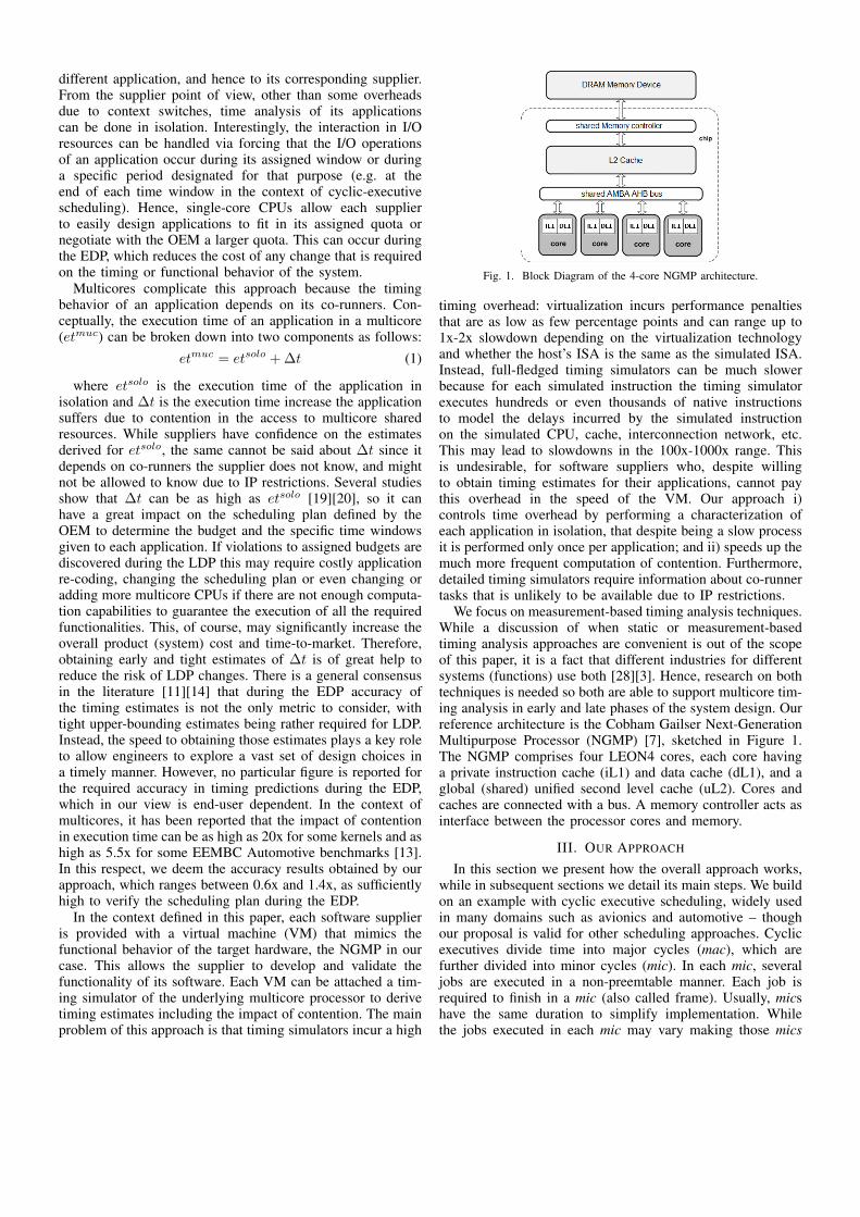
Fig. 1. Block Diagram of the 4-core NGMP architecture.

timing overhead: virtualization incurs performance penaltiesthat are as low as few percentage points and can range up to1x-2x slowdown depending on the virtualization technologyand whether the host’s ISA is the same as the simulated ISA.Instead, full-fledged timing simulators can be much slowerbecause for each simulated instruction the timing simulatorexecutes hundreds or even thousands of native instructionsto model the delays incurred by the simulated instructionon the simulated CPU, cache, interconnection network, etc.This may lead to slowdowns in the 100x-1000x range. Thisis undesirable, for software suppliers who, despite willingto obtain timing estimates for their applications, cannot paythis overhead in the speed of the VM. Our approach i)controls time overhead by performing a characterization ofeach application in isolation, that despite being a slow processit is performed only once per application; and ii) speeds up themuch more frequent computation of contention. Furthermore,detailed timing simulators require information about co-runnertasks that is unlikely to be available due to IP restrictions.

We focus on measurement-based timing analysis techniques.While a discussion of when static or measurement-basedtiming analysis approaches are convenient is out of the scopeof this paper, it is a fact that different industries for differentsystems (functions) use both [28][3]. Hence, research on bothtechniques is needed so both are able to support multicore tim-ing analysis in early and late phases of the system design. Ourreference architecture is the Cobham Gailser Next-GenerationMultipurpose Processor (NGMP) [7], sketched in Figure 1.The NGMP comprises four LEON4 cores, each core havinga private instruction cache (iL1) and data cache (dL1), and aglobal (shared) unified second level cache (uL2). Cores andcaches are connected with a bus. A memory controller acts asinterface between the processor cores and memory.

III. OUR APPROACH

In this section we present how the overall approach works,while in subsequent sections we detail its main steps. We buildon an example with cyclic executive scheduling, widely usedin many domains such as avionics and automotive – thoughour proposal is valid for other scheduling approaches. Cyclicexecutives divide time into major cycles (mac), which arefurther divided into minor cycles (mic). In each mic, severaljobs are executed in a non-preemtable manner. Each job isrequired to finish in a mic (also called frame). Usually, micshave the same duration to simplify implementation. Whilethe jobs executed in each mic may vary making those mics

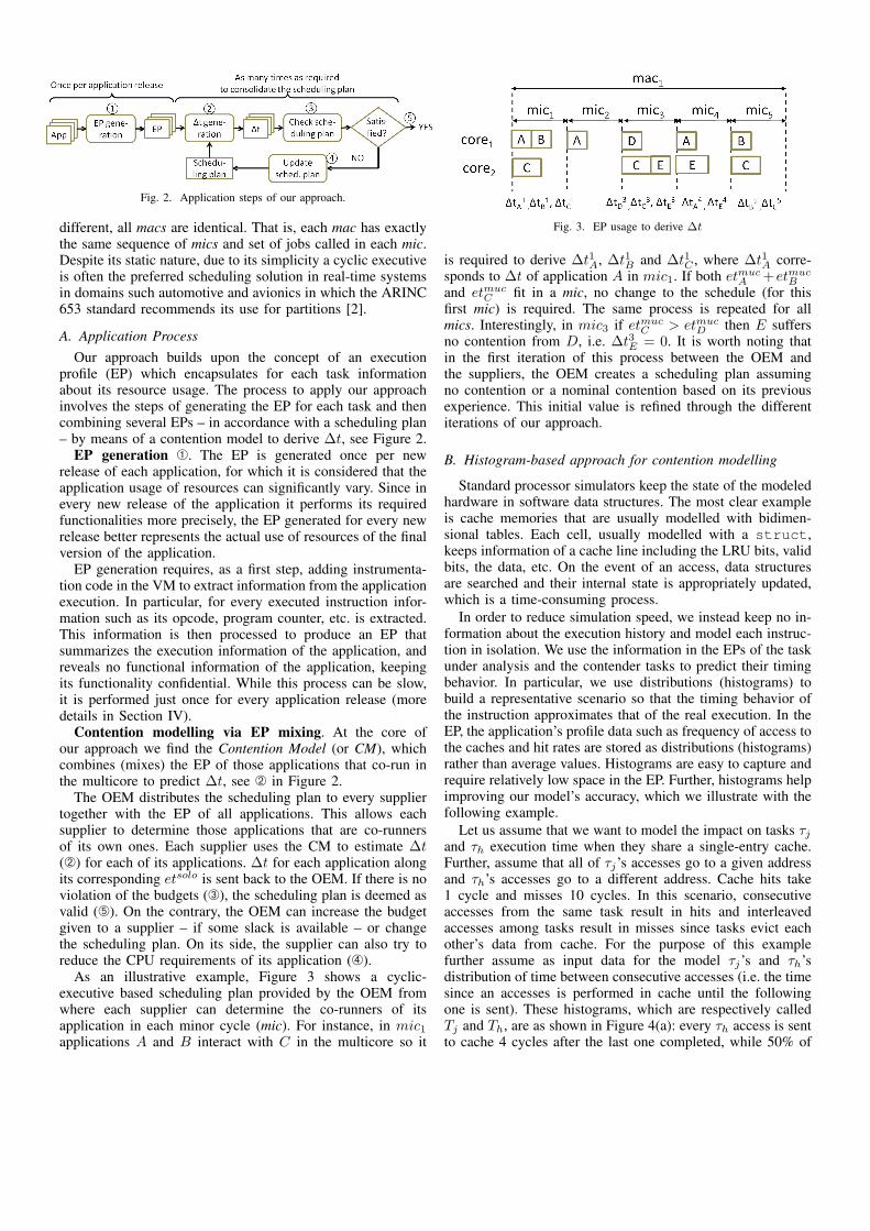
Fig. 2. Application steps of our approach.

different, all macs are identical. That is, each mac has exactlythe same sequence of mics and set of jobs called in each mic.Despite its static nature, due to its simplicity a cyclic executiveis often the preferred scheduling solution in real-time systemsin domains such automotive and avionics in which the ARINC653 standard recommends its use for partitions [2].

A. Application ProcessOur approach builds upon the concept of an execution

profile (EP) which encapsulates for each task informationabout its resource usage. The process to apply our approachinvolves the steps of generating the EP for each task and thencombining several EPs – in accordance with a scheduling plan– by means of a contention model to derive ∆t, see Figure 2.

EP generation À. The EP is generated once per newrelease of each application, for which it is considered that theapplication usage of resources can significantly vary. Since inevery new release of the application it performs its requiredfunctionalities more precisely, the EP generated for every newrelease better represents the actual use of resources of the finalversion of the application.

EP generation requires, as a first step, adding instrumenta-tion code in the VM to extract information from the applicationexecution. In particular, for every executed instruction infor-mation such as its opcode, program counter, etc. is extracted.This information is then processed to produce an EP thatsummarizes the execution information of the application, andreveals no functional information of the application, keepingits functionality confidential. While this process can be slow,it is performed just once for every application release (moredetails in Section IV).

Contention modelling via EP mixing. At the core ofour approach we find the Contention Model (or CM), whichcombines (mixes) the EP of those applications that co-run inthe multicore to predict ∆t, see Á in Figure 2.

The OEM distributes the scheduling plan to every suppliertogether with the EP of all applications. This allows eachsupplier to determine those applications that are co-runnersof its own ones. Each supplier uses the CM to estimate ∆t(Á) for each of its applications. ∆t for each application alongits corresponding etsolo is sent back to the OEM. If there is noviolation of the budgets (Â), the scheduling plan is deemed asvalid (Ä). On the contrary, the OEM can increase the budgetgiven to a supplier – if some slack is available – or changethe scheduling plan. On its side, the supplier can also try toreduce the CPU requirements of its application (Ã).

As an illustrative example, Figure 3 shows a cyclic-executive based scheduling plan provided by the OEM fromwhere each supplier can determine the co-runners of itsapplication in each minor cycle (mic). For instance, in mic1applications A and B interact with C in the multicore so it

Fig. 3. EP usage to derive ∆t

is required to derive ∆t1A, ∆t1B and ∆t1C , where ∆t1A corre-sponds to ∆t of application A in mic1. If both etmuc

A +etmucB

and etmucC fit in a mic, no change to the schedule (for this

first mic) is required. The same process is repeated for allmics. Interestingly, in mic3 if etmuc

C > etmucD then E suffers

no contention from D, i.e. ∆t3E = 0. It is worth noting thatin the first iteration of this process between the OEM andthe suppliers, the OEM creates a scheduling plan assumingno contention or a nominal contention based on its previousexperience. This initial value is refined through the differentiterations of our approach.

B. Histogram-based approach for contention modelling

Standard processor simulators keep the state of the modeledhardware in software data structures. The most clear exampleis cache memories that are usually modelled with bidimen-sional tables. Each cell, usually modelled with a struct,keeps information of a cache line including the LRU bits, validbits, the data, etc. On the event of an access, data structuresare searched and their internal state is appropriately updated,which is a time-consuming process.

In order to reduce simulation speed, we instead keep no in-formation about the execution history and model each instruc-tion in isolation. We use the information in the EPs of the taskunder analysis and the contender tasks to predict their timingbehavior. In particular, we use distributions (histograms) tobuild a representative scenario so that the timing behavior ofthe instruction approximates that of the real execution. In theEP, the application’s profile data such as frequency of access tothe caches and hit rates are stored as distributions (histograms)rather than average values. Histograms are easy to capture andrequire relatively low space in the EP. Further, histograms helpimproving our model’s accuracy, which we illustrate with thefollowing example.

Let us assume that we want to model the impact on tasks τjand τh execution time when they share a single-entry cache.Further, assume that all of τj’s accesses go to a given addressand τh’s accesses go to a different address. Cache hits take1 cycle and misses 10 cycles. In this scenario, consecutiveaccesses from the same task result in hits and interleavedaccesses among tasks result in misses since tasks evict eachother’s data from cache. For the purpose of this examplefurther assume as input data for the model τj’s and τh’sdistribution of time between consecutive accesses (i.e. the timesince an accesses is performed in cache until the followingone is sent). These histograms, which are respectively calledTj and Th, are as shown in Figure 4(a): every τh access is sentto cache 4 cycles after the last one completed, while 50% of

(a) Tj and Th for τj and τh (b) τh’s execution time prediction

Fig. 4. Example of use of the histogram-based modelling approach

τj requests are sent one cycle after the previous one and theother 50% every 7 cycles after the previous one completes.

Average. If we use information about average both τj andτh are assumed to send one request to the cache at the samerate of every 4 cycles. As a result all accesses would interleaveand be misses. If τj performs 100 accesses, its predictedexecution time would be 1,000 cycles. This fails to capturethe fact that τj has a bimodal distribution, which means thatthe number of requests from τj among requests of τh varies:it can be 0, 1, 2 or 3 and hence some accesses can be hits.

Histogram. With the approach based on histograms, for ev-ery τj access we derive the time since the last access accordingto its histogram. To that end we define a random variable Xmodelling frequencies in the histogram as probabilities. Forinstance, Tj is the random variable capturing the distributionof cycles between consecutive τj’s accesses.

We refer to a realization of the random variable (distribu-tion) X as x, i.e. the name of the random variable but inlower case. Hence, tj is one particular value obtained fromthe distribution Tj . For instance, to obtain tj we generate arandom number (r) between 0 and 1, so r ∈ [0, 1). Given thatthe time between accesses for τj is 1 or 7 cycles with 50%probability each, tj is 1 or 7 as follows:

tj =

{1 cycle if (r < 0.5)7 cycles if (r ≥ 0.5)

This process for obtaining one value from a random vari-able, which can be performed for histograms with any numberof points and density, is called realization. We represent it asx = rand(X), that for the case of the time between accessesis tj = rand(Tj).

Coming back to the example in Figure 4, the histogrambased approach results in τj and τh experiencing hits andmisses – as it would be expected based on their frequencyof access. To obtain the predicted execution time for τj , weperform several runs of the model. In each run, the accessdelay of each access is obtained by performing one realizationof Tj (e.g., tj = 7) and as many as needed of Th to determinehow many accesses of τh occurred since the previous accessof τj . The estimate obtained for the execution time distributionfor τj is as shown in Figure 4(b). We observe that the resultingdistribution captures the fact that the alignment between tasks’accesses impacts each task’s execution time. The averageexecution time is 779 cycles instead of 1,000 as with theaverage-based model.

Our results in Section VI show for real benchmarks thattaking averages instead of considering the histogram leads tohigh inaccuracies since accesses interleave systematically inthe same way despite the fact that, in reality, they interleave

TABLE IBASIC NOTATION.

in many different ways. Instead, histogram-based interleavingcaptures tasks’ access interleaving much more accurately.

C. Restricted Access Interleaving Information

A key element in our approach is that we assume noinformation about the distribution (over time) of the accessesof a given program to hardware resources. For instance, for τjin Figure 4(a) we know 50% of the accesses are sent 1 cycleafter the previous completes and the other 50% 7 cycles. Ourmodel does not record, for instance, information about whetherthose accesses concentrate on the initial phase of the executionof the program or at the end, that is, how they interleave withother task instructions. If we assume that τj and τh run inparallel it could be the case that all τj accesses occur beforethose of τh, so in reality they are not going to suffer inter-taskcontention in cache. Likewise, we do not record informationabout whether τj accesses of the different types interleave.

There are several reasons behind this choice. (i) Keepingtime-dependent distribution information would increase thesize of EP, since we could not summarize it in a histogrambut we would need to keep the exact sequence of accessesand how they interleave over time. This would also resultin more complex and time-consuming modelling. (ii) Thisapproach would also affect time composability [23][22] sinceprovided contention bounds would be specific to how requestsinterleave, which changes when tasks suffer any type of shift.

Since our model aims at predicting the worst-case con-tention among tasks, not the average, whenever two taskspartially overlap in the scheduling plan we pessimistically

increase their etmuc assuming they fully overlap and hence,suffer continuously high contention. Despite this adds somepessimism, it simplifies EP and makes the CM lighter – whichis critical since the CM is used in an iterative manner to adjustthe scheduling plan, so it has to incur a small slowdown.

D. Notation and ParametersThe main parameters used for our model are those in Table I.

We introduce some of them in this section, while others arepresented as they are used. In Table I, starting bottom up, weobserve that parameters provide cache, per-instruction, per-access information and per-task information. The latter is fur-ther broken down into cache, time and instruction informationof the task. For cache information of the task we use theconvention metric− cache− task: metric are the initials ofthe metric described (in capital letters to mean it is a randomvariable, i.e. histogram); cache is cache initial, that for theNGMP is i for the instruction cache, d for the data cache andu for the unified L2 cache. Finally task is the task id that isadded as subindex. For instance, Kdj is the stack distance ofthe accesses to dL1 of task τj . When we talk about a cachein general we omit the cache initial, e.g Kj .

We introduce some of Table I’s parameters via the examplesequence in Figure 5. For each access we report its address,accessed cache set and the time in which it happens.

• Time between accesses to the same set (TS) capturesthe time between accesses targeting the same set. Forinstance, accesses #2 and #8 to addresses @D and @Erespectively, are consecutive accesses to set 1 (set1).They occur in cycles 4 and 25 respectively, which resultsin a time between accesses to the same set of 21 cycles.

• Set distance (E) for a given set seti is the numberof other sets (different than seti but not necessarilyunique) accessed since the last time seti was accessed.For instance, access #2 in Seq1 accesses set1, whichis accessed again by access #8. In between there are 5accesses to sets different than set1, hence set distanceequals 5 for #8.

• Stack distance (K). The stack distance of an access @Al

is defined as the number of unique (i.e. non-repeated)addresses mapped to the same set where @Al is mappedand that are accessed between @Al and the previousaccess to it, i.e. @Al−1. Note that stack distance issimilar to the concept of reuse distance, though the latterdoes not break down accesses per set. For instance, inSeq1 the accesses to set0 are (AABCBAAABC) withstack distances (∞0∞∞120012) respectively. The stackdistance of a task τj (Kj) is built from the stack distancesof its accesses.

It is worth noting that common eviction cache policiessuch as LRU have the stack property [18], which determineswhether a given address is still in cache. For LRU, the focusof this paper, each set in a cache can be seen as an LRU stackwith lines sorted based on their last access cycle. The first lineof the LRU stack is the Most Recently Used (MRU) and thelast is the LRU. Interestingly, i) the position of a line in theLRU stack defines its stack distance; ii) those accesses witha stack distance smaller than or equal to the number of cacheways (w) result in a hit and vice versa; and iii) the sensitivityof the access of τj to be evicted from cache by accesses of a

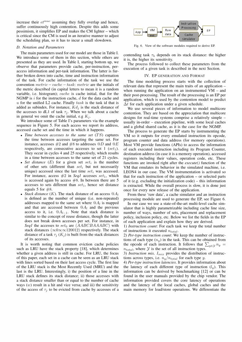
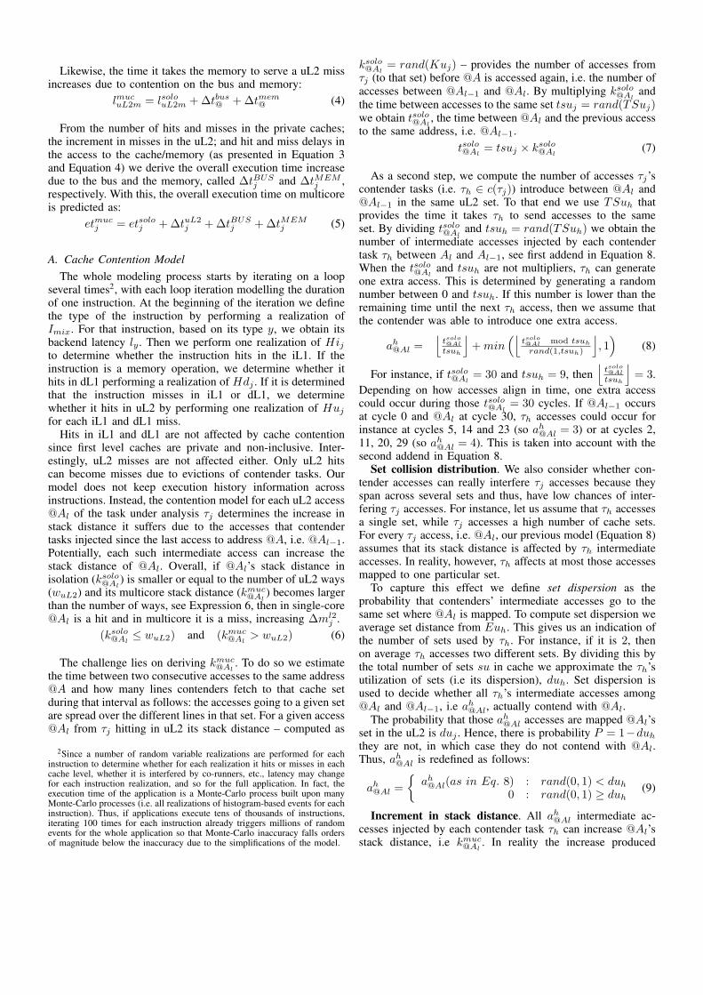
Fig. 6. View of the software modules required to derive EP.

contending task τh depends on its stack distance: the higherit is, the higher its sensitivity.

The process followed to collect these parameters from theexecution of a given task is described in the next Section.

IV. EP GENERATION AND FORMAT

The time modeling process starts with the collection ofrelevant data that represent the main traits of an application –when running the application on an instrumented VM – andtheir post-processing. The result of the processing is an EP perapplication, which is used by the contention model to predict∆t for each application under a given schedule.

We use several pieces of information to model multicorecontention. They are based on the appreciation that multicoredesigns for real-time systems comprise a relatively simple –usually in-order – execution pipeline, with some local cachesand a global shared cache, as it is the case for the NGMP.

The process to generate the EP starts by instrumenting theVM so it outputs for every emulated instruction its opcode,program counter and data address (for memory operations).Most VM provide functions (APIs) to access the informationof each executed instruction including its Program Counter,destination address (in case it is a memory operation), accessedregisters including their values, operation code, etc. Thesefunctions are invoked right after the execute() function of theVM that emulates its behavior in the simulated machine, i.e.LEON4 in our case. The VM instrumentation is activated sothat for each instruction of the application – or selected partsof it (e.g. excluding the initialization code) – this informationis extracted. While the overall process is slow, it is done justonce for every new release of the application.

From these ‘raw data’, a cache simulator and an instructionprocessing module are used to generate the EP, see Figure 6.

In our case we use a state-of-the-art multi-level cache sim-ulator that is highly parametrizable including cache line size,number of ways, number of sets, placement and replacementpolicy, inclusion policy, etc. Below we list the fields in the EPof each application and explain how they are derived.1) Instruction count: For each task we keep the total numberof instructions it executed ntotal.2) Per-type instruction count: We keep the number of instruc-tions of each type (ny) in the task. This can be obtained fromthe opcode of each instruction. It follows that

∑y∈Y ny =

ntotal, where Y is the set of all instruction types.3) Instruction mix. Imix provides the distribution of instruc-tions across types, i.e. ny/ntotal for each type y.4) Per-type instruction latencies. It provides information aboutthe latency of each different type of instruction (ly). Thisinformation can be derived by benchmarking [12] or can befound in the user manuals provided by the chip vendor. Theinformation provided covers the core latency of operationsand the latency of the local caches, global caches and themain memory for load/store operations. We differentiate the

Access number 1 2 3 4 5 6 7 8 9 10 11 12 13 14 15 16 17address @A @D @A @B @F @C @B @E @A @A @F @A @B @E @C @A @F

accessed set s0 s1 s0 s0 s2 s0 s0 s1 s0 s0 s2 s0 s0 s1 s0 s0 s2time 1 4 10 14 16 20 22 25 32 36 40 41 43 50 56 58 60TSj 0 0 9 4 0 6 2 21 10 4 24 5 2 25 13 2 20Ej ∞ ∞ 1 0 ∞ 1 0 5 1 0 5 1 0 5 1 0 5Kj ∞ ∞ 0 ∞ ∞ ∞ 1 ∞ 2 0 0 0 1 0 2 2 0

Fig. 5. Access Sequence Seq1 generated by a task τj

TABLE IIOPERATION TYPES IN THE NGMP AND THEIR ASSUMED LATENCIES

operation type jitter min-max latency Assumed latencyint. short latency NO 1 1int. long latency YES 1-35 35

control NO 1 1fp. short latency NO 4 4fp. long latency YES 16-25 25

following instruction types (Y) since they are common inseveral RISC architectures: integer short latency (e.g., add,cmp), integer long latency (e.g., idiv, imult), control (e.g.,bne), floating point short latency (e.g., fpadd, fpmult),floating point long latency (e.g., fpdiv and fpsqrt) andmemory operations (e.g., ld and st). Some of these types canbe further divided. For instance, the floating point long latencytype can be split into divisions (fpdiv) and square roots(fpsqrt) since the execution time of these two instructiontypes can be quite different.

It is noted that each instruction instance may suffer variabil-ity in its execution time due to two factors. First, input-datadependence that occurs when instructions such as floating-point division take variable latency depending on the partic-ular values (input-data) operated. And second, pipeline statedependence: in this case, a given instruction may have variablelatency depending on its predecessor instructions. In our aimto model the worst-case we handle these sources of jitter byassuming as the latency for every type an upperbound to thoselatencies. This provides an upperbound to the execution ofthe instruction. This incurs relatively low inaccuracy whilekeeping the model simple and fast. For the NGMP, whichhas mostly a stall-free pipeline, so removing pipeline-statedependences, Table II shows the latency we assume in ourmodel for every instruction type.5) Local caches information: For the local caches, our cachesimulator provides the hit rate. In particular for each τj wekeep Hij and Hdj .6) Global caches information: As for the local caches, werecord information on the hit rate of the application for theglobal caches, i.e. Huj for the NGMP.7) Inter-access latency: For every core instruction executedwe have its latency ly . For instruction and cache accesses thecache simulator is used to determine whether they hit/miss inthe different cache levels, for which we have an associatedlatency. With this information, for every two accesses to uL2we can predict the execution time of the instructions betweenthem, and hence we can derive the time between consecutiveaccesses. The histogram (TSuj) is derived by counting howmany times each latency occurs between two consecutive uL2accesses to the same set.8) Kuj and Euj : From the cache simulator it is straightfor-ward to derive stack distance and set distance since we havethe memory operations accessing uL2 and the set they access.

TABLE IIISPECIFIC INFORMATION IN THE EXECUTION PROFILE

Hij , Hdj , Huj cache hit rates (miss rates derived as (1−Hxj))TSuj Time between accesses going to the same set in uL2Kuj uL2 stack distance of τi (including all data accesses)Euj uL2 set distance of τi (including all data accesses)Imix Percentage of instructions of each typentotal,ny Total and per-type instruction countly Nominal back-end latency per instruction typeetsoloj τj ’s execution time in isolation

9) Solo performance . In our environment, software suppliersare provided with a virtualized environment (e.g. for theSPARC based NGMP in our case) that runs on a host platform(e.g. x86) where etsolo – that is the first addend in Equation 5– cannot be derived. We derive etsolo by applying a simpleapproach in which for each instruction we add its front-end(of the pipeline) latency and its back-end latency.

etsoloj =∑y∈Y

[ny × (fend(y) + bend(y))] (2)

Instruction’s front-end latency depend on whether theyhit or miss in iL1 and uL2. For each of these scenariostheir associated latency is different. Whether an instructionhits/misses in cache is provided by the cache simulator. Forcore operations, such as add or mult, ly gives an estimate oftheir execution time in the back-end. For memory operationssuch as load or store, their back-end latency also dependson whether they hit or miss in dL1 and uL2.Overall, the EP generation deploys a high-level cache sim-ulator and some extra modules that process the informationcoming from the instrumentation of the VM. As a result weobtain an EP that is the input for contention modelling. Theinformation in the EP is summarized in Table III.

V. CONTENTION MODELING

In this section we explain the main elements of our con-tention model as well as the assumptions on which it holds.

The main shared resources we consider in our target ar-chitecture (see Figure 1) are the uL2 cache, the bus and thememory bandwidth. For the former we explain our contentionmodel in Section V-A and for the latter two in Section V-B.Our model keeps no state information about executed instruc-tions, i.e. it models each instruction in isolation.

First, the cache contention model predicts the increment innumber of misses that τj suffers due to the contention createdby its co-runners, ∆muL2

j . Then it derives the executiontime increment (∆tuL2

j ) caused by those ∆muL2j hits in the

execution in isolation that become misses due to its co-runners.In a second step, we account for the impact on the bus and

the memory controller that each access suffers when accessingthose resources. The access latency of each uL2 hit is increasedby the contention on the bus:

lmucuL2h = lsolouL2h +∆tbus@ (3)

Likewise, the time it takes the memory to serve a uL2 missincreases due to contention on the bus and memory:

lmucuL2m = lsolouL2m +∆tbus@ +∆tmem

@ (4)

From the number of hits and misses in the private caches;the increment in misses in the uL2; and hit and miss delays inthe access to the cache/memory (as presented in Equation 3and Equation 4) we derive the overall execution time increasedue to the bus and the memory, called ∆tBUS

j and ∆tMEMj ,

respectively. With this, the overall execution time on multicoreis predicted as:

etmucj = etsoloj +∆tuL2

j +∆tBUSj +∆tMEM

j (5)

A. Cache Contention ModelThe whole modeling process starts by iterating on a loop

several times2, with each loop iteration modelling the durationof one instruction. At the beginning of the iteration we definethe type of the instruction by performing a realization ofImix. For that instruction, based on its type y, we obtain itsbackend latency ly . Then we perform one realization of Hijto determine whether the instruction hits in the iL1. If theinstruction is a memory operation, we determine whether ithits in dL1 performing a realization of Hdj . If it is determinedthat the instruction misses in iL1 or dL1, we determinewhether it hits in uL2 by performing one realization of Huj

for each iL1 and dL1 miss.Hits in iL1 and dL1 are not affected by cache contention

since first level caches are private and non-inclusive. Inter-estingly, uL2 misses are not affected either. Only uL2 hitscan become misses due to evictions of contender tasks. Ourmodel does not keep execution history information acrossinstructions. Instead, the contention model for each uL2 access@Al of the task under analysis τj determines the increase instack distance it suffers due to the accesses that contendertasks injected since the last access to address @A, i.e. @Al−1.Potentially, each such intermediate access can increase thestack distance of @Al. Overall, if @Al’s stack distance inisolation (ksolo@Al

) is smaller or equal to the number of uL2 ways(wuL2) and its multicore stack distance (kmuc

@Al) becomes larger

than the number of ways, see Expression 6, then in single-core@Al is a hit and in multicore it is a miss, increasing ∆ml2

j .(ksolo@Al

≤ wuL2) and (kmuc@Al

> wuL2) (6)

The challenge lies on deriving kmuc@Al

. To do so we estimatethe time between two consecutive accesses to the same address@A and how many lines contenders fetch to that cache setduring that interval as follows: the accesses going to a given setare spread over the different lines in that set. For a given access@Al from τj hitting in uL2 its stack distance – computed as

2Since a number of random variable realizations are performed for eachinstruction to determine whether for each realization it hits or misses in eachcache level, whether it is interfered by co-runners, etc., latency may changefor each instruction realization, and so for the full application. In fact, theexecution time of the application is a Monte-Carlo process built upon manyMonte-Carlo processes (i.e. all realizations of histogram-based events for eachinstruction). Thus, if applications execute tens of thousands of instructions,iterating 100 times for each instruction already triggers millions of randomevents for the whole application so that Monte-Carlo inaccuracy falls ordersof magnitude below the inaccuracy due to the simplifications of the model.

ksolo@Al= rand(Kuj) – provides the number of accesses from

τj (to that set) before @A is accessed again, i.e. the number ofaccesses between @Al−1 and @Al. By multiplying ksolo@Al

andthe time between accesses to the same set tsuj = rand(TSuj)we obtain tsolo@Al

, the time between @Al and the previous accessto the same address, i.e. @Al−1.

tsolo@Al= tsuj × ksolo@Al

(7)

As a second step, we compute the number of accesses τj’scontender tasks (i.e. τh ∈ c(τj)) introduce between @Al and@Al−1 in the same uL2 set. To that end we use TSuh thatprovides the time it takes τh to send accesses to the sameset. By dividing tsolo@Al

and tsuh = rand(TSuh) we obtain thenumber of intermediate accesses injected by each contendertask τh between Al and Al−1, see first addend in Equation 8.When the tsolo@Al

and tsuh are not multipliers, τh can generateone extra access. This is determined by generating a randomnumber between 0 and tsuh. If this number is lower than theremaining time until the next τh access, then we assume thatthe contender was able to introduce one extra access.

ah@Al =⌊tsolo@Al

tsuh

⌋+min

(⌊tsolo@Al mod tsuh

rand(1,tsuh)

⌋, 1)

(8)

For instance, if tsolo@Al= 30 and tsuh = 9, then

⌊tsolo@Al

tsuh

⌋= 3.

Depending on how accesses align in time, one extra accesscould occur during those tsolo@Al

= 30 cycles. If @Al−1 occursat cycle 0 and @Al at cycle 30, τh accesses could occur forinstance at cycles 5, 14 and 23 (so ah@Al = 3) or at cycles 2,11, 20, 29 (so ah@Al = 4). This is taken into account with thesecond addend in Equation 8.

Set collision distribution. We also consider whether con-tender accesses can really interfere τj accesses because theyspan across several sets and thus, have low chances of inter-fering τj accesses. For instance, let us assume that τh accessesa single set, while τj accesses a high number of cache sets.For every τj access, i.e. @Al, our previous model (Equation 8)assumes that its stack distance is affected by τh intermediateaccesses. In reality, however, τh affects at most those accessesmapped to one particular set.

To capture this effect we define set dispersion as theprobability that contenders’ intermediate accesses go to thesame set where @Al is mapped. To compute set dispersion weaverage set distance from Euh. This gives us an indication ofthe number of sets used by τh. For instance, if it is 2, thenon average τh accesses two different sets. By dividing this bythe total number of sets su in cache we approximate the τh’sutilization of sets (i.e its dispersion), duh. Set dispersion isused to decide whether all τh’s intermediate accesses among@Al and @Al−1, i.e ah@Al, actually contend with @Al.

The probability that those ah@Al accesses are mapped @Al’sset in the uL2 is duj . Hence, there is probability P = 1−duh

they are not, in which case they do not contend with @Al.Thus, ah@Al is redefined as follows:

ah@Al =

{ah@Al(as in Eq. 8) : rand(0, 1) < duh

0 : rand(0, 1) ≥ duh(9)

Increment in stack distance. All ah@Al intermediate ac-cesses injected by each contender task τh can increase @Al’sstack distance, i.e kmuc

@Al. In reality the increase produced

depends on the number of accesses generated by τh andtheir stack distance. In one extreme of the spectrum, whenall intermediate accesses have stack distance equal to zerothey go to the same cache block (line), so they increase kmuc

@Al

just by one. In the other extreme, when all accesses go todifferent addresses (blocks) their impact on the stack distanceis as high as the number of accesses. For instance, let usassume that τh generates 4 accesses between @Al and @Al−1.If their stack distance is 0, they all access the same address(e.g., BBBB). If their stack distance is 1, then they access 2different addresses (e.g., BCBC). In particular, the number ofdifferent addresses accessed by τh is determined by the stackdistance (plus one), but never exceeding the total number ofah@Al intermediate accesses. Note that for each τh access weobtain its stack distance as rand(Kuh).

We take into account the impact of the accesses gener-ated by τh on @Al’s stack distance (∆kh@Al) as shown inEquation 10. This equation assumes that all accesses havethe same stack distance. This simplification still builds uponstack distance histograms, but reduces the cost of performinga realization of Kuh for each ah@Al intermediate access.

∆kh@Al = min(ah@Al, rand(Kuh) + 1) (10)

By accounting for the increase in the stack distance of ksolo@Al

caused by each τh we derive its kmuc@Al

:

kmuc@Al

= ksolo@Al+

∑τh∈c(τj)

∆kh@Al (11)

Outcome. The addition of the stack distance of Al inisolation (ksolo@Al

) and ∆ah@Al for each contender provides kmuc@Al

.As expressed in Equation 6, if ksolo@Al

is smaller or equal to thenumber of uL2 cache ways and kmuc

@Alis larger than the number

of ways, that particular access is predicted to be a hit whenτj runs in isolation and becomes a miss when it runs with itscontenders, increasing ∆tuL2

j .

B. Bus and memory (BM) and (MM)

The bus and memory contention models for the NGMPtake into account that bus accesses are not split3, so that thebus contention model also captures contention tasks suffer inmemory. If bus transactions were split, allowing requests fromdifferent tasks contend on the bus and in memory in parallel,then the model should be duplicated for both resources.

Our model estimates the contention experienced by task τjon the bus (and memory) that we refer to as ∆tBUS

j and ismeasured in cycles. For that purpose we derive (1) how longτj spends using the bus, etbusuL2

j , which already factors in theimpact of contention misses derived with the cache contentionmodel; (2) the bus utilization of its contenders ubusc(j); (3)the probability than on an access to the bus τj finds it availableabusj ; to finally (4) obtain ∆tBUS

j .The time τj spends on the bus, etbusuL2

j , is obtained byadding the time spent serving uL2 cache hits and misses inisolation and the time to serve the uL2 contention misses.

3In the NGMP the bus is not relinquished until the access is served eitherby the uL2 cache or memory.

etbusuL2j =((nsolo

uL2h −∆muL2j )× luL2hit) +

((nsolouL2m +∆muL2

j )× luL2miss)

= (nsolouL2h × luL2hit) +

(nsolouL2m × luL2miss) +(

∆muL2j × (luL2miss − luL2hit)

)(12)

where nsolouL2h and nsolo

uL2m correspond to the number of uL2hits and misses in isolation, respectively; and ∆muL2

j of theuL2 hits in isolation become miss due to contention. Therefore,for the bus utilization, etbusuL2

j factors in uL2 hits and missesapplying the cache contention model, but not their impact onthe bus contention. We obtain the total solo execution timeplus the effect of cache contention analogously, by adding theimpact of the extra misses due to contention:

etuL2j = etsoloj +∆muL2

j × (luL2miss − luL2hit) (13)

By dividing the time spent using the bus by etuL2j = etsoloj

for a given task, we obtain its bus occupancy in isolationfactoring in cache contention, ubusuL2

j .

ubusuL2j =

etbusuL2j

etuL2j

(14)

Then, we add the utilization of all contenders of τj to obtainthe accumulate utilization they cause.

ubusc(j) =∑

τh∈c(τj)

ubusuL2h (15)

Note, however, that ubusc(j) can be higher than 100%. Forinstance, let assume τj has two contenders, τh and τm, eachwith bus utilization of 60%. This results in a bus utilizationof ubusc(j) = 1.2 that will be even higher when accountingfor τj utilization in isolation. It is obvious that contentionwill increase the time window since total bus utilization ofτj and its contenders cannot exceed 100%. The time windowincreases by the true contention that the other tasks cause onτj . However, the actual impact of contention on the bus isthe result of the model. For instance, recalling the previousexample, the impact of τh and τm bus accesses will increaseτj execution time, thus increasing bus availability (samenumber of accesses over a larger time window). However,such increased bus availability is already needed to computethe time window, thus creating a circular dependence.

To break this dependence, we upper-bound contention im-pact in the time window with the total utilization of the othertasks. See the right addend of Equation 16, where the timewindow available is 1 (available utilization in isolation) plusthe time that other tasks access the bus (ubusc(j)). Hence,the actual bus utilization is approximated by dividing theutilization of the other tasks by the total time window. τj findsthe bus available (abusj) when it is not being used by others.

abusj = 1−ubusc(j)

1 + ubusc(j)(16)

In the example before, if ubusc(j) = 1.2 then abusj = 0.45,so this is the probability assumed for τj accesses to find the

bus available. Note that in the equation above, if the other tasksdid not use the bus, abusj = 1. Conversely, if the utilizationof the other tasks was huge, then abusj ≈ 0.

Finally, by dividing 1 by the probability of success weobtain how often a bus access from τj tries to access the busto get it. Then we multiply this probability by the time spenton the bus in isolation etbusuL2

j to obtain the total time spenton the bus due to contention, ∆tBUS

j , as shown below.

∆tBUSj =

(1

abusj

)× etbusuL2

j (17)

C. Simplifications of the Model

Our model balances accuracy in its prediction and the exe-cution time overhead to run it. Results presented in Section VIshow that our model achieves a good balance between both.In this section we list the main simplifications in our modelto speed it up and how they impact accuracy.

General approach. The most remarkable assumption in ourmodels is that we take frequencies observed when character-izing applications as probabilities. However, events such ascache hits/misses do not have a randomized nature as it wouldbe required to attach probabilities to their occurrence. For thesake of simplicity we make this assumption for any processto limit the complexity of the cache model.

Core model. In general our model does not work with thetemporal distribution of events. For instance, we assume thatinstructions of each type are equidistant in the code. Despitewe have histograms we do not consider how instructions aredistributed over time. For computing processor core time, weover-approximate the execution time of each instruction in thecore instead of tracking pipeline and data dependences, thatis, we assume the longest latency of a jittery instruction, e.g.for the NGMP we assume that fplong, i.e. fp long-latencyinstruction we assume, always takes 25 cycles when in realityit can take either 16 or 25 cycles depending on the input valuesoperated. This heavily simplifies the processor core time modelwith low impact on accuracy.

Cache model. For the cache model, stack distances andset distances are not maintained per set, but we have onestack distance histogram and one set distance histogram forthe whole cache. Alternatively, to increase accuracy we couldkeep information in a per-set basis, but this would add somenon-negligible complexity to the model, would increase theamount of information recorded by a factor of s (the numberof sets in cache), and would make results dependent on theactual sets (and so memory locations) of the different tasks.Another source of innacuracy is that we average set distanceto approximate set dispersion.

Bus model. In the bus model there are two main sources ofinaccuracy. First, when determining the bus availability for atask the time window assumed is upper-bounded. Second andmore important, our bus model assumes that bus accesses areblocking, i.e. they stall the processor pipeline. However, theLEON4 cores in the NGMP have a store buffer able to managea pending store without stalling the pipeline. Since dL1 cachesare write-through in the LEON4 core, write operations to uL2are abundant. Hence, the bus contention effect will not be aslinear as assumed, resulting in under-estimations of the model.

As shown in the result section, the overall accuracy of themodel is acceptable as execution time estimates to be usedduring the EDP, while it incurs low execution time overhead.

Addressable unit. For sake of simplicity we have assumedin our explanations that each access corresponds to a cacheline. When the addressable unit is smaller than a cache line,accesses to different addresses can be mapped to the samecache line. This has no impact on our previous formulation.For instance, let us assume the sequence (A,A,B,C,B,A),in which B and C go to the same line. We can simply abstractthis sequence as (A,A,B,B,B,A), hence considering that theaccess to C corresponds to another access to B, so cache stackdistances would be (∞ 0 ∞ 0 0 0 1). This allows us applyingthe formulation presented.

VI. REALIZATION AND EVALUATION ON THE NGMPIn this section we show how we realize our models for the

NGMP [7], whose general block diagram is shown in Figure 1.

A. Experimental FrameworkBasics on the NGMP. In the space domain the NGMP [7],

whose latest implementation is the GR740 [8], is being con-sidered by the European Space Agency (ESA) for its futuremissions. Each LEON4 core comprises a seven-stage scalarin-order pipeline. The NGMP has four cores, each comprisinginstruction (iL1) and data (dL1) first-level caches. Each coreaccesses to the L2 cache through an AHB AMBA bus.

Floating point. The FPU has two possible data paths for FPoperations: one for FP divisions and square roots, and one forthe rest of FP operations. This last data path is fully pipelined,and has a latency of 4 cycles and, under ideal conditions, athroughput of one cycle. The data path for divisions and squareroots is not pipelined, so the throughput of these operations isequal to their latency.

Bus: The interconnection bus is a 128-bit AHB AMBA busarbitrated with round-robin policy. It has 5 masters (4 cores,and I/O master) and 2 slaves (L2 cache and I/O slave). Asexplained before, the bus-split feature is not implemented inthe GR-CPCI-LEON4-N2X [5], meaning that once a core hasits access to the bus granted, no other device can access thebus until the access is performed. Our model has been fit tothis architecture where bus-split is not available.

Memory model: Every core has 16KB 4-way 128-set iL1and dL1 caches, implementing write-through, write no allocatepolicies. The unified L2 cache is shared by all the cores in theprocessor. It is a 256KB 4-way 2048-set cache. It uses writepolicy is copy-back/write allocate. Cores also include somestore buffers capabilities.

Simulator. We have modeled this architecture on an en-hanced version of the SoCLib simulation framework [25] andvalidated that execution time measurements obtained in thesimulator are on average within 3% of those obtained in thereal board for the N2X implementation of the NGMP [5]for the EEMBC benchmark suite [21] as well as some spaceapplications. We use the execution times obtained from thesimulator as reference to assess the accuracy of our model.

Benchmarks. We use a solid set of benchmarks to assessour contention model.

EEMBC automotive. The EEMBC automotive benchmarksuite [21] is a well-known benchmark suite in the real-time domain, and it is particularly useful for evaluating the

(a) Common cases (b) Extreme cases

Fig. 7. Accuracy of the cache contention model

capabilities of embedded microprocessors, compilers, and theassociated embedded system implementations. The diversityof this suite ensures that designers can use combinationsof EEMBC workloads to make effective design choices. Inparticular we use these benchmarks: aifirf (AF), aiifft(AT), bitmnp (BI),cacheb (CB), canrdr (CN), idctrn(ID), iirflt (II), puwmod (PU), rspeed (RS).

European Space Agency benchmarks. We use representativebenchmarks of ESA on-board software. In particular, the On-board Data Processing (OB) and DEBIE (DE) benchmarks.

• On-board Data Processing contains the algorithms usedto process raw frames coming from the state-of-the-artnear infrared (NIR) HAWAII-2RG detector [16], alreadyused in real projects, like the Hubble Space Telescope todetect cosmic rays.

• DEBIE is the software that controls an instrument, whichwas carried on PROBA-1 satellite, to observe micro-meteoroids and small space debris by detecting impactson its sensors, both mechanically and electrically.

Stressing Kernels. In order to also stress our model inhigh contention situations, we have implemented five re-source stressing kernels [13][24] that create high contention inshared resources. Those benchmarks include l2full (U) andl2half (H), which traverse continuously an array occupyingthe whole L2 and half of it, respectively; l2miss (M) andl1miss (L), which continuously miss on their respectivecaches; and mixed-8-12-80 (E), which executes a specificmixture of instructions (8% stores, 12% loads and 80% adds).

Workloads. We run four-task workloads. For the first taskwe use our model to estimate its execution time bound.This first task is either a EEMBC AutoBench benchmark oran ESA benchmark. The other three (contending) tasks inthe workload are l2full, l2half, l2miss, l1miss ormixed-8-12-80. This creates a stressful scenario in whichwe can fairly assess the accuracy of the predictions our model.Table IV summarizes the workloads used in this paper.

Metrics. We evaluate the accuracy provided by our model interms of the increment in the number of L2 misses (∆muL2

i ),bus time (∆tBUS

i +∆tMEMi ) and the overall execution time

in multicore (etmuc). For each of these three metrics wemeasure accuracy as PredictedV alue

ActualV alue . Hence the closer to onethe better, with values above one showing that the model over-approximates and values below one that the model under-approximates. For each four-task workload, we measure theaccuracy in estimating the contention of its first task. As shownin Table IV we create eight workloads for each EEMBC Auto-motive and the ESA benchmarks. We show the distribution of

TABLE IVWORKLOADS USED FOR EVALUATION

BENCHMARK 8 WORKLOADS IN WHICH IT RUNSAF (LLL), (LLH), (LHL), (HLL), (HLH), (HHL), (LHH), (ULL)AT (UUU), (UMU), (MUU), (UUM), (MMU), (MUM), (UMM), (MMM)BI (UUU), (UMU), (MUU), (UUM), (MMU), (UMM), (MUM), (MMM)CB (LUU), (UUU), (ULU), (UUL), (HUU), (MUU), (UHU), (UMU)CN (ULU), (UUL), (LUU), (HUU), (UHU), (UUH), (MUL), (ULM)DE (MUU), (UMU), (UUU), (UUM), (MMU), (MUM), (UMM), (MMM)ID (UUU), (UMU), (MUU), (UUM), (MMU), (UMM), (MUM), (MMM)II (LLL), (LLH), (LHL), (HLL), (LHH), (LEL), (HLH), (LLE)OB (UUU), (UMU), (MUU), (UUM), (MMU), (MUM), (UMM), (MMM)PU (UUU), (UMU), (MUU), (UUM), (LUU), (ULU), (UUL), (UMM)RS (LLL), (LLH), (LHL), (HLL), (LEL), (LLE), (ELL), (HLH)

Fig. 8. Accuracy of the bus contention model

the accuracy across the eight workloads with a boxplot, thusshowing the median, the quantiles, maximum and minimumvalues and outliers.

B. Experimental ResultsCache Contention Model. As we can see in Figure 7(a)

∆muL2i is accurately estimated for several benchmarks and

somehow overestimated for others. The largest deviation aredue to the fact that our cache contention model assumesthat stack and set distances are homogeneous across sets forthe sake of simplicity. However, this is not always the caseand, in fact, our l2full and l2half synthetic kernelsare specifically designed to stress all cache sets and half ofthem, respectively, so that heterogeneous behavior across setsproduces large inaccuracies in our model.

The case of the three benchmarks in Figure 7(b) is com-pletely different since ∆muL2

i is in the range [10, 100]. In thiscase, benchmarks suffer in the order of dozens extra misses inL2 due to contention, which is negligible for those benchmarksexecuting millions of instructions. Hence, although our modeloverestimates ∆muL2

i by a factor of 10-20x, this only repre-sents accounting for around of 1,000 extra L2 misses whoseimpact in the total execution time is negligible.

It can also be observed that the cache contention modelleads to an overestimation of ∆muL2

i . The main reason isthe fact that our model assumes that cache accesses arehomogeneously distributed in time. However, in reality theytypically occur in bursts. Thus, if bursts of all different tasksoccur simultaneously, the model is accurate but if, instead,not all of them overlap completely (the common case) realinterference is lower than estimated because the number ofinterfering accesses from other tasks during a burst of the taskunder analysis is lower than predicted.

Average-Based Model. For comparison purposes we ob-tained results for the cache contention model using averagevalues rather than histograms. Our results show that for all theworkloads listed in Table IV the average-based model detects

Fig. 9. Performance accuracy of the complete model. Results havebeen normalized w.r.t. the actual measurements.

almost no contention. This occurs because dividing averagevalues by the number of sets du, as done in Equation 9,leads to very low predicted interferences among tasks. Thisproduces contention predictions as low as 0.0034, that is withan inaccuracy of almost 100% (1− 0.0034 = 0.9966).

Bus Contention Model. For bus contention, shown inFigure 8, we observe a variety of behaviors across benchmarks.Although such contention is somehow overestimated for fewbenchmarks, it is typically underestimated for most of them.This effect is particularly noticeable for aiifft, debieand obdp. As explained before, the NGMP processor hasstore buffers that are able to hide part of the latency ofstores. However, since stores occur in bursts, whenever theyoccur in a short period of time they can produce performancedegradations much higher than linear. For instance, it has beenproven that execution time may grow by a factor of 20x in theNGMP with just 4 cores due to the (bad) interaction of storeoperations in the different cores [13]. How to better capturethis effect in our bus contention model without incurring highoverhead is still part of our future work.

Putting it all together: Multicore Execution Time. Wehave also analyzed the accuracy of our performance estimateswhen considering all contention models and assumptionstogether. The accuracy in determining etsolo is high withpredictions in the range [1.02, 1.23] for all benchmarks.

Results are shown in Figure 9. We observe that the accuracyof the estimates is mostly dominated by bus contention inthe NGMP. The main reason is the fact that the differencebetween L2 hit and L2 miss latencies is relatively low (9versus 23 cycles) and only affects ∆muL2

i , whereas theimpact of bus contention affects all load misses in L1 and allstore instructions given that DL1 is write-through. Therefore,inaccuracies due to the effect of the store buffer in terms ofbus contention dominate the results.

Overall, our simple analytical model is able to keep perfor-mance estimates in the range [0.6, 1.4] w.r.t. the real perfor-mance in the NGMP. These are accurate results for executiontime estimations for early-design phases. The accuracy of ourmodel allows system designers to really take into accountmulticore contention in the design choices made (e.g. decidingthe scheduling plan).

Model Execution Time Overhead. To be usable in EDP,the execution time overhead of our model should be low.

To produce the ‘raw data’ from the VM as presented inFigure 2, we introduce instrumentation instructions to readinformation about the particular instruction under execution.The number of instructions to add is relatively low: three

(a) Time required by the EP generation

(b) Time to perform one estimation of the multicore contention

Fig. 10. Average overheads of our contention prediction model.

instructions in our case to read opcode, program counter anddata address. From the raw data we run the cache simulatorand process instructions to generate the EP. Figure 10(a) showsthe execution time of this EP generation step, which is run justonce per application. If the application has several releaseswhose resource-usage profile is expected to change, this stepis repeated once for each of those releases. The duration of thisstep depends on the length of the program. For the EEMBCand the real ESA benchmarks, whose execution is in the orderof dozens millions of instructions, in the worst case this steptakes around 80 seconds. On average EP generation requiresaround 20 seconds across all benchmarks, which is reasonablyshort given the low frequency with which this step executes.

Figure 10(b) shows the execution time overhead of con-tention models, once EP information has been produced. Theduration of this step is the most important for the feasibility ofour approach. This is so because, once the EPs are generated,the system designer needs short turn-around time of the modelsto be able to evaluate different design choices. We observe thatpredicting the multicore performance of an application in aworkload requires as low as 120ms on average, which enablesa vast design space exploration of various system parametersby system designers.

VII. RELATED WORKS

The focus of timing analysis techniques in the literature forEDP has been on single-core architectures. To our knowledge,the work presented in this paper is the first addressing thechallenge of providing timing estimates in EDP for multicores.

Some approaches for single-core architectures work on theassumption that the target processor and/or the correspondingcompilation toolchain is available, while others do not. Whenthe target processor is not available, several techniques existto derive timing estimates that help deciding the hardwareplatform that best satisfies system requirements [11][26] aswell as sizing it. The approach consists in compiling the sourcecode for a given set of potential target ISAs. For each of theISA there is a parameterizable processor simulator (model)from which timing information is gathered. The model allowschanging parameters with high impact on timing such as cache

configuration [26]. Then program information (e.g. paths)obtained from the executable and timing from the generic pro-cessor model are combined to approximate programs executiontime. In our case the target ISA and processor are fixed, sosuch an approach would not be necessary.

Other approaches do not work at the binary level but atthe source code level, or an intermediate representation level,which are available earlier in the design cycle of the system.In some cases, timing is integrated in high level modellingenvironments such as Matlab/Simulink [9]. The ultimate goalis providing the developer knowledge of the worst-case “as thecode is written” [10]. In all cases the focus is on single-corearchitectures, while our focus is on multicore contention.

In many of the approaches above one of the main challengeslies in deriving a light, yet accurate, timing (cost) model forindividual instructions or sequences of them. Some papers [10]assume a WCET-friendly processor design, such as the JavaOptimized Processor (JOP). This simplifies the timing modelsince the processor is predictability aware. Other papers pro-pose methods to derive a timing model from measurementsof representative code extracts on the target processor. For in-stance, authors in [17] work on the concept of C-source-levelabstract machine which is calibrated based on measurementsto match a target real hardware. In this line, [14] proposes thetiming model code level that combines measurements and aregression model to perform timing estimates of source code.In this latter work, the timing (cost) model is built, i.e. it is notassumed as an input. In both cases the focus is on constructsthat frequently appear on the target programs.

While previous works focus on single-core processors,our focus is on multicore specific aspects. In particular thecontention in the access to hardware shared resources. Formulticore, it could be possible to run the program underanalysis against a set of resource stressing kernels (rsks) whichput high load on the shared resources [13], [24]. This wouldprovide a good estimation of the program execution time underheavy (extreme) load conditions. However, it has been shownthat this approach leads to inflated execution time estimates,up to 20x bigger than programs’ execution time in isolation,which makes it impractical to obtain accurate execution timeapproximations during EDP.

Previous works show that, while exact bounds are requiredin LDP, during EDP, instead, approximations to those boundare needed [11][14]. Some accuracy is traded to speed up theestimation process so that engineers can make design spaceexploration taking into account timing. To our knowledge, noparticular figure is reported on accuracy required in EDP. Formulticores several works show that the impact of contentioncan up to 20x for some kernels and up to 5.5x for someEEMBC benchmarks [13]. In this context, we deem theaccuracy results obtained by our approach (between 0.6x and1.4x) as sufficiently precise.

VIII. CONCLUSIONS

In this paper we present a new timing model for early designstages able to predict in a fast manner the performance ofapplications when the target (virtual) platform is multicorebased. They key idea behind our model is the generation ofan execution profile (EP) for each application that software

suppliers can share without revealing IP, yet allowing perfor-mance analysis of multicore contention. This paper describeshow EP are generated and how they are combined to predictthe performance of applications under particular schedule. Ourresults show that useful estimates can be obtained extremelyfast since generating an EP takes few seconds and evaluatinga schedule less than 0.2 seconds for the NGMP architecture.

ACKNOWLEDGEMENT

This work has received funding from the European SpaceAgency under Project Reference AO/1−7722/13/NL/LvH ,and has also been supported by the Spanish Ministry ofScience and Innovation grant TIN2015-65316-P. Jaume Abellahas been partially supported by the MINECO under Ramon yCajal postdoctoral fellowship number RYC-2013-14717.

REFERENCES

[1] Guidelines and methods for conducting the safety assessment processon civil airborne systems and equipment. ARP4761, 2001.

[2] ARINC Specification 653: Avionics Application Software Standard Stan-dard Interface, Part 1 and 4, 2012.

[3] J. Abella et al. WCET analysis methods: Pitfalls and challenges on theirtrustworthiness. In SIES, 2015.

[4] Aeroflex Gaisler. Quad Core LEON4 SPARC V8 Processor - LEON4-NGMP-DRAFT - Data Sheet and Users Manual, 2011.

[5] Aeroflex Gaisler. LEON4-N2X Data Sheet, 2013.[6] AUTOSAR. Technical Overview V2.0.1, 2006.[7] Cobham Gaisler. NGMP Preliminary Datasheet Version 2.1, May 2013.[8] Cobham Gaisler. Quad Core LEON4 SPARC V8 Processor - GR740-

UM-DS-D1 - Data Sheet and Users Manual, 2015.[9] Raimund Kirner et al. Fully automatic worst-case execution time

analysis for matlab/simulink models. In ECRTS, 2002.[10] Trevor Harmon et al. Fast, interactive worst-case execution time analysis

with back-annotation. IEEE Trans. Industrial Informatics, 8(2), 2012.[11] C. Ferdinand et al. Integration of code-level and system-level timing

analysis for early architecture exploration and reliable timing verifica-tion. In ERTS2, 2010.

[12] G. Fernandez et al. Increasing confidence on measurement-basedcontention bounds for real-time round-robin buses. In DAC, 2015.

[13] Mikel Fernandez et al. Assessing the suitability of the ngmp multi-coreprocessor in the space domain. In EMSOFT, 2012.

[14] J. Gustafsson et al. Approximate worst-case execution time analysis forearly stage embedded systems development. In SEUS, 2009.

[15] M. M. Irvine and A. Dartnell. The use of emulator-based simulators foron-board software maintenance. In Data Systems in Aerospace (DASIA),volume 509 of ESA Special Publication, 2002.

[16] Andreas Jung and Pierre-Elie Crouzet. The H2RG infrared detector:introduction and results of data processing on different platforms.Technical report, European Space Agency, 2012.

[17] R. Kirner and P. Puschner. A simple and efficient fully automatic worst-case execution time analysis for model-based application development.In Workshop on Intelligent Solutions in Embedded Systems, 2003.

[18] R. L. Mattson, J. Gecsei, D. R. Slutz, and I. L. Traiger. Evaluationtechniques for storage hierarchies. IBM Syst. J., 9(2), June 1970.

[19] M. Paolieri et al. An Analyzable Memory Controller for Hard Real-TimeCMPs . Embedded System Letters (ESL), 2009.

[20] Zheng Pei Wu et al. Worst case analysis of DRAM latency in multi-requestor systems. In RTSS, 2013.

[21] Jason Poovey. Characterization of the EEMBC Benchmark Suite. NorthCarolina State University, 2007.

[22] Peter Puschner and Martin Schoeberl. On Composable System Timing,Task Timing, and WCET Analysis. In WCET Analysis Workshop, 2008.

[23] P. Puschner et al. Towards Composable Timing for Real-Time Soft-ware. In Workshop on Software Technologies for Future DependableDistributed Systems, 2009.

[24] Petar Radojkovic et al. On the evaluation of the impact of sharedresources in multithreaded cots processors in time-critical environments.ACM TACO, 2012.

[25] SoCLib. -, 2003-2012. http://www.soclib.fr/trac/dev.[26] http://www.absint.com/timingprofiler. Timing Profiler. AbsInt.[27] http://www.gmv.com/en/aeronautics/products/air/. Robust Partition

Safety-Critical Real-Time Operating System. GMV.[28] Wilhelm R. et al. The worst-case execution-time problem overview of

methods and survey of tools. ACM TECS, 7:1–53, May 2008.