Improving Prediction of Wireline Data Using Artificial

i

Improving Prediction of Wireline Data Using Artificial Neural

Network

By

Ahmed Mohamad Essam Aly Rafaat

14710

Supervised By

Dr. Sia Chee Wee

A project dissertation submitted

In partial fulfilment of the requirement for the

Bachelor of Engineering (Hons)

(Petroleum Engineering)

JANUARY 2015

University Teknologi PETRONAS

Bandar Seri Iskandar

31750 Tronoh

Perak Darul Ridzuan

ii

CERTIFICATION OF APPROVAL

Improving Prediction of Wireline Data Using Artificial Neural

By

Ahmed Mohamad Essam Aly Rafaat

14710

Petroleum Engineering

A project dissertation submitted

In partial fulfilment of the requirement for the

Bachelor of Engineering (Hons)

(Petroleum Engineering)

JANUARY 2015

Universiti Teknologi PETRONAS

Bandar Seri Iskandar

31750 Tronoh

Perak Darul Ridzuan

Approved by,

…………………….

(Dr. Sia Chee Wee)

Project Supervisor

iii

CERTIFICATION OF ORIGINALITY

This is to certify that I am responsible for the work submitted in this project, that the

original work is my own except as specified in the references and

acknowledgements, and that the original work contained herein have not been

undertaken or done by unspecified sources or persons.

Written by,

……………………………

(Ahmed Mohamad Essam Aly Rafaat, 14710)

iv

ABSTRACT

This paper is dedicated to investigate the capabilities of artificial neural network

(ANN) to improve prediction of petrophysical properties. Furthermore, this project is

intended to test capability of network to predict the logging tools readings based on

other tools readings.

For petrophysical data prediction, it will be limited to predicting values of porosity

by comparing predicted values from different models and values obtained from core

data.

Data obtained for core is considered to be the most accurate representation of

petrophysical data. Hence, it is used as a reference data for testing capabilities of the

model and training ANN networks.

On the other hand, for logs data, the data sets are limited to these six (6)

fundamental logs; transient time (DT), gamma ray (GR), neutron porosity (NPHI),

bulk density (RHOB), resistivity deep (ILD) and resistivity shallow (ILM).

In this research Gullfaks field data is utilized for training the model, and improving

its prediction. Also, it will be used to test the model and its ability to predict the logs

and porosity values.

Then, this paper takes it further to test obtained ANN models on other fields. For this

purpose, Kansas City log data is utilized to predict capability of model to predict

logs reading and to prove the obtained models are universal models and not limited

to the trained reservoir.

Also, optimization of models formulated will be utilized on two fields. First field is

utilizing the input data to statistically cover all possibilities of outputs whereas the

other field is to optimize the model to use less nodes and reduce running time to

estimate outputs.

Finally, the research final model will be tested if it can be utilized on different

reservoirs. In this research, the data from Gullfaks field is utilized to obtain the

models and data from Kansas City for testing final model.

Results show that there is a true empirical formula among the logs and the accurate

determination of the formula is strongly related to the quality of data obtained

v

ACKNOWLEDGEMENT

First I would like to thank to Allah the Almighty, The Most Merciful, for all His

guidance throughout my learning process in turning this project into a reality.

Heartfelt gratitude and appreciation to my Final Year Project (FYP) supervisor, Dr.

Sia Chee Wee for his continuous help and encouraging in gaining invaluable

experience for this project.

Last but not least, my greatest appreciation goes to those who have assisted me

directly or indirectly starting from the beginning of the project. All of the

experiences and lessons obtain shall not be wasted and hopefully, which will lead me

to be a successful and flexible Petroleum Engineer.

vi

TABLE OF CONTENTS

CHAPTER 1 BACKGROUND ................................................................................. 1

1. Wireline brief history ...................................................................... 1

2. Introduction of Artificial Neural Network in Petroleum

Engineering ......................................................................................... 2

3. Problem Statement .......................................................................... 4

CHAPTER 2 LITERATURE REVIEW ................................................................... 7

1. Different Wireline Interpretation Models .................................... 7

2. Sources Of Petrophysical Uncertainty ......................................... 8

3. Artificial Neural Network Model ................................................. 9

CHAPTER 3 METHODOLOGY ............................................................................ 12

1. Data Description ......................................................................... 12

2. Organizing the data .................................................................... 12

3. Training and model evaluation .................................................. 16

4. ANN Model Structure ................................................................. 20

5. Training Different Models .......................................................... 21

CHAPTER 4 RESULTS AND DISCUSSION ...................................................... 22

CHAPTER 5 CONCLUSION AND REOCOMMENDATIONS .......................... 39

Chapter 6

REFERENCES………………………………………………………………………..

38

CHAPTER 7 APPENDIX ......................................................................................... 1

APPENDIX – I – VBA code to extract data from .las files. .............. 1

APPENDIX – II – VBA code to organise data from directory of .las

files. ...................................................................................................... 2

vii

APPENDIX – III – C++ code to extract selective logs data from

directory of .las files. ........................................................................... 3

APPENDIX – IV – C++ code to elimante logs without needed input

data from directory of .las files. .......................................................... 4

viii

Table of figures

Figure 1: Steps of Coring Process (Halliburton Drilling Plug System)

Figure 2: DT-log Distribution

Figure 3: GR-Log Distribution

Figure 4: ILD-Log Distribution

Figure 5: ILM -Log Distribution

Figure 6: NPHI-Log Distribution

Figure 7: RHOB Distribution

Figure 8: Kansas City Well Description

Figure 9: MATLAB TOOL BOX TRAINING STEPS (1)






Figure 14: ANN Model

Figure 15: Comparison between different models prediction

Figure 16: COMPARISON OF RANGE OF ERROR

Figure 17: Comparison between DT model -3- (top) and model -5- (bottom) in Error

distribution

Figure 18: Comparison between NPHI model -3- (top) and model -5- (bottom) in

Error distribution

Figure 19: Comparison between NPHI model -3- (top) and model -5- (bottom) in

Error distribution

Figure 20: Comparison between ILD model -3- (top) and model -5- (bottom) in Error

distribution

Figure 21: Comparison between RHOB model -3- (top) and model -5- (bottom) in

Error distribution

Figure 22: Comparison between ILM model -3- (top) and model -5- (bottom) in

Error distribution

Figure 23: Trend of DT prediction from Gullfaks field

Figure 24: Trend of GR prediction from Gullfaks field

Figure 25: Trend of ILD prediction from Gullfaks field

Figure 26: Trend of ILM prediction from Gullfaks field

ix

Figure 27: Trend of NPHI prediction from Gullfaks field

Figure 28: DT Model prediction from Kansas City Data

Figure 29: GR Model prediction from Kansas City Data

Figure 30: ILD Model prediction from Kansas City Data

Figure 31: ILM Model prediction from Kansas City Data

Figure 32: NPHI Model prediction from Kansas City Data

1

CHAPTER 1

INTRODUCTION

1.0 BACKGROUND

The goal behind Wire-line data is to have continues representation of formation

physical properties, lithology and fluids content. Wire-line data is essential to obtain

critical information to form proper reservoir model. The more accurate the data

collected from wire-line logging, the more accurate is the reservoir model prediction.

1.1 Wireline brief history

First electric wireline log reading goes back to 1927 in a small oil field at

Pechelbronn, Alsace, France. The electrical resistivity log was recorded using a

SONDE which measures formation resistivity within every few intervals. The first

resistivity continuous reading was introduced in mid-1950.

In 1930, the anisotropy dip meter was introduced to the logging tools. One year later,

the spontaneous potential (SP) log was introduced by Marcel and Conrad, the

Schlumberger brothers, and then included among resistivity logs. In 1946, the photo

clinometer was introduced. Those were the first logging tools available.

However since then, wireline tools development became more diverse and complex.

Nowadays, geologists use huge combination of logging tools to determine different

lithological properties to estimate petrophysical properties which in its turn aid in

volumetric calculations of reserves.

1.2 Uncertainties within well-log data

Solution of any technical problem is derived from connections between various

quantities and parameters. The relations between various quantities can be explicit or

implicit. (Walstrom, 1967, December 1)

According to Walstrom, the petrophysical properties estimation entirely depend on

the quantities which estimation is calculated from. Any inaccuracy in acquiring data

of those properties will propagate error in the estimation process.

Determined variables, are parameters quantified with high accuracy and degree of

precision. Accuracy and degree of precision of determined variables depend on

2

statistical description of data accumulated on specific variable during the data

development stage.

Uncertainties evolve from difficulties in directly measuring quantities. Within

petroleum engineering, the fact is that petroleum engineers do not have direct access

to the reservoir, which leads to difficulties in measuring the reservoir petrophysical

properties. Such type of complexity result in great contribution in reservoir

uncertainties that widely affect reserves estimation. (Walstrom, 1967, December 1)

To determine porosity, logging tools undergoes huge uncertainties, since the tool

measurement is defined by equations where porosity is a factor in the equation.

Thus, uncertainty exists.

As an example for simplification, porosity can be defined using the following three

equations from different logging tools:

1) Neutron Porosity :

𝜙𝑛 = (1 − 𝜙𝑒)𝜙𝑁𝑚𝑎 + 𝜙𝑒[𝑆𝑤 × 𝜙𝑁𝐹1 + (1 − 𝑆𝑊)𝜙𝑁𝐹2]................... (1)

2) Density Porosity :

𝜌𝑏 = (1 − 𝜙𝑒)𝜌𝑁𝑚𝑎 + 𝜙𝑒[𝑆𝑤 × 𝜌𝐹1 + (1 − 𝑆𝑊)𝜌𝑁𝐹2]........................ (2)

3) Sonic Porosity :

∆𝑇𝑛 = (1 − 𝜙𝑒)∆𝑇𝑁𝑚𝑎 + 𝜙𝑒[𝑆𝑤 × ∆𝑇𝐹1 + (1 − 𝑆𝑊)∆𝑇𝐹2].................. (3)

The most efficient way to estimate real porosity values from those logs is by

correlating the three equation obtained using readings from different logs which will

result in near accurate data compared to the porosity within lithology. Correlation

between the three equations reduces or eliminates uncertainties involved in well log

data readings.

1.3 Introduction of Artificial Neural Network in Petroleum Engineering

Artificial Neural Network (ANN) is the attempt to simulate real human neurons

work model in solving non-linear relations and patterns.

Ali made a study to show that ANN can be used in variety of applications within

petroleum industry like geology and geophysics to determine reserves estimation and

3

mineral identification from well log (Ali, 1994, January 1). In formation evaluation,

ANN has been used also used in predicting carbonate permeability and prediction of

pore pressure from well logs data.

Kumoluyi conducted a study on how to use higher order neural networks for

different petroleum engineering applications. They used well-log interpretation to

establish a continuity of stratigraphic units and multiphase flow analysis to

determine flow regime for given flow conditions, also on using seismic data to

compress large amount of data without compromising vital information. (Kumoluyi

et al, 1994).

Arora used parallel systems of ANN to compute different processes, using high

count of input data and built relationship between them. (Arora, 10 January 2014).

Kumar used ANN to predict permeability and porosity of specific reservoir from

well log and seismic data with accuracy of 92 %.( Kumar, 2012).

On the other hand, ANN is widely used outside petroleum engineering in various

field and proven to be highly effective. In medicine it is used to Modeling and

Diagnosing the Cardiovascular System

Neural Networks are used experimentally to model the human cardiovascular

system. Diagnosis can be achieved by building a model of the cardiovascular system

of an individual and comparing it with the real time physiological measurements

taken from the patient. If this routine is carried out regularly, potential harmful

medical conditions can be detected at an early stage and thus make the process of

combating the disease much easier.

ANN also is used in security systems as a face recognition to specific people where

it can grant access or trigger an alarm based on the face captured from the

surveillance.

What makes ANN very popular is its parallel processing capabilities, where in

normal computer processors code is run step by step, or command after command,

on the other hand ANN have capabilities to run different commands parallel at the

same time and speed. The difference is each neuron runs a small and simple

operation where the combined effort of all neurons is summed and the final answer

required from the model is obtained.

4

2. PROBLEM STATEMENT

One of the main methods to determine reservoir petrophysical properties is by using

wireline data. Wireline data is used to determine many critical petrophysical

properties such as porosity, permeability and water saturation. The increase of

reservoir complexity causes high uncertainties in estimation of reservoir

petrophysical

properties. Uncertainties can be due to wide range of error such as error in readings

from tool while data gathering, offset in equipment calibration and wrong statistical

data handling. With uncertainty in inputs a definite error propagate towards the

outputs.

To determine the reserves volume within the reservoir the following formula is

generally utilized.

𝑅𝑒𝑠𝑒𝑟𝑣𝑒𝑠 𝑣𝑜𝑙𝑢𝑚𝑒 = (𝐵. 𝑉 × 𝑁𝑇𝐺 × Φ × (1 − S𝑤) × 𝑅. 𝐹 )/𝐵𝑜..…………….. (4)

To solve the formula, we need to obtain porosity (Φ), Water Saturation (S𝑤) and Net

to Growth (NTG) from wireline data. Each of porosity, water saturation and net to

growth is the associated uncertainties which cause error and deviation from real

reservoir petrophysical properties.

Coring provides the only valid representation of the formation. It’s the only means of

direct measurement. All other methods such as well logs require interpretation.

While conventional well logs play an important part in reservoir identification, only

coring can ensure reliable correlation of those logs to the actual subsurface

conditions. And for the most advanced analysis, only core samples can yield critical

data such as porosities, permeability, and saturations.

Coring cost is calculated from the following equation:

𝐶𝑐 =𝐶𝑏+ 𝐶𝑠+ 𝐶𝑟×( 𝑡𝑡+ 𝑡𝑐+𝑡𝑟𝑐)

𝐿×

1

𝑅𝑐……………………… (4)

Cc = coring cost per foot.

Cb = cost of core bit.

Cs = cost of coring service from a

service company.

Cr = rig day rate.

tt = trip time, hour.

tc = core recovering time, hour.

trc = core barrel handling time, hour.

L = length of core recovered, ft.

Rc = percentage of core recover, %.

5

Where the average cost per foot range between 500 to 900 USD per foot depending

on rig rate and bit used for coring operations.

On the other hand, running wireline can be significantly cheaper that it reaches 80 to

180 USD per foot.

With current decrease of oil prices and search for oil in unconventional locations, the

need for cost saving techniques is highly needed by the industry to continue

supplying the world with needed energy. By reducing the coring cost to almost zero

and minimize the logging tool running cost lead to almost 20 to 25% cost reduction

in the overall development plan.

3. OBJECTIVE AND SCOPE OF STUDY

New approach is required to estimate reservoir petrophysical properties that will lead

to cost reduction. ANN presents a robust approach to find such complex

mathematical relations due to its huge capacity to recognize patterns and complex

nonlinear relations among different variables by learning through training.

Figure 1: Steps of Coring Process (Halliburton Drilling Plug System)

6

The objective of this paper is to attempt to utilize the power of ANN in finding

complex non-linear relations between various well log inputs, correlate uncertainties

associated and estimate petrophysical properties of reservoir.

Due to time and source constraints, this study is limited to the following scope:

1) Formulating empirical formulas between the following logs:

a. Raw Bulk Density Correction well-log (RHOB).

b. Sonic Log well-log (DT).

c. Gamma Ray Log well-log (GR).

d. Raw Deep Induction Resistivity well-log (ILD).

e. Raw medium Induction Resistivity well-log (ILM).

f. Neutron Porosity well-log (NPHI).

2) Estimation of Porosity using correlation between correlated logs and core

data.

The training and testing data will be limited to Gullfaks well-log data and validation

of model global application will be limited to Kansas City well-log data to prove that

formulas obtained from scope one can be applied in different reservoirs.

7

CHAPTER 2

LITERATURE REVIEW

2.1 DIFFERENT WIRELINE INTERPRETATION MODELS

Different physical properties of reservoir lithology can be estimated using different

log tools. The process involves measuring different physical properties by sending

down the tools into borehole. Then on surface, geologists with the aid of advance

computer software, interpret values recoded by the tool on a log-log papers. Using

specific models and equations, the petrophysical properties is estimated from data

recorded by logging tools.

As an example, evaluating porosity from well-log data. Porosity can be determined

by three different types of logging tool that measure different lithology’s physical

property such as sonic, density and neutron log.

2.1.1 Sonic log

Sonic log measures interval of time needed by sound to travel from one point to

another through compressional sound wave through formation along borehole axis.

(Brock, 1986). The interval of time taken by the sound to travel from specific point

on the tool through formation to another point, is called transit time (Δt), and usually

measured in µsec/ft or µsec/m depending on imperial or SI units.

From sonic logs, porosity can be determined by Wyllie’s Time-average formula:

Φ = Δ𝑡𝑙𝑜𝑔− Δ𝑡𝑚𝑎𝑡𝑟𝑖𝑥

Δ𝑡𝑓−Δ𝑡𝑚𝑎𝑡𝑟𝑖𝑥………………………………………………………….. (5)

Or by Raymer-Hunt-Gardner’s formula:

Φ = 5

8×

Δ𝑡𝑙𝑜𝑔− Δ𝑡𝑚𝑎𝑡𝑟𝑖𝑥

Δ𝑡𝑙𝑜𝑔…………………………………………………….... (6)

Assuming that we know the transit time for the matrix with high accuracy.

2.1.2 Density log

Density log uses gamma ray from a chemical source. Density log interacts with

formation’s elements on the electron level. Porosity is determined by count of

returning gamma rays. The count measures density of electrons within formation.

Two energy levels are measured to estimate various characteristics. First energy

8

level is high energy gamma that utilizes Compton’s scattering concept to estimate

bulk density and therefore, Porosity. The second energy level is low energy gamma

which utilizes photoelectric effect to estimate formation lithology. Low energy

gamma is independent from porosity value and formation fluids content. (Brock,

1986)

Porosity is evaluated from the following formula:

Φ = 𝜌𝑚𝑎−𝜌𝑏

𝜌𝑚𝑎−𝜌𝑓…………………………………………………………… (7)

Assuming matrix and fluid density need to be known.

2.1.3 Neutron log

Neutron log uses neutrons emitted form chemical source, usually a mixture of

Americium-Beryllium. A neutron is almost as heavy as a proton. Hydrogen atom has

one single proton in the nuclei. Bombardment of the hydrogen nuclei by neutron rays

causes hydrogen and neutron to collide. Average energy loss due to neutron-

hydrogen collisions is almost 50% of original neutron energy. Water, oil and gas are

rich with hydrogen atoms, which make them very easily detectable using neutron

logs. By estimating fluid content within formation, geologists can easily estimate the

volume of fluid occupying pores within formation, hence estimate the porosity

(Brock, 1986).

2.2 SOURCES OF PETROPHYSICAL UNCERTAINTY

Estimation of the real reservoir porosity from a single log cause low reading

accuracy and precision. Estimation of the real reservoir porosity from a single log,

results in many errors in reservoir reserves volume estimation. This is credited to

many uncertainties and errors associated with each log readings. In geophysics, a

common practice by engineers is to use cross-plot to correlate for major errors and

uncertainties in well log readings, due to formation and borehole complexity.

In case of sonic log, porosity readings can be affected in case of borehole

enlargement. The transit time recorded will be deviated from real transit time value

within formation, due to space between sonic tool and borehole wall. If formation

contains fractures or faults, this will lead sonic waves to pass through two different

formation densities leading to a shift in transit time reading that cause the porosity

9

estimation at that particular depth to be deviated from real value. Those are some

examples of uncertainties associated with formation complexity. Other errors are due

to measuring process, such as excessive logging speed which causes road noise.

For density logs, one example of uncertainty can be noticed from type of mud used

in drilling, borehole roughness and variations in borehole diameter across the depth.

Those variations and uncertainties are mainly due to barrier between tool and

formation or measuring tool lost contact with formation.

Neutron log is less effected by rough borehole which makes it good for reducing

errors in other logs readings. Sonic log is highly affected by high temperature and

pressure. Sonic log is also effected by borehole salinity and mud cake formation. All

those types of uncertainty is due to the complex model of reservoir borehole. Other

uncertainties evolve from data collection process, measuring tool calibrations and

many others.

With every model, combined readings from different logs lead to different type of

uncertainty quantification. Using combination of logs to correlate for error and

uncertainty is tedious long process which impact the reserves estimation

economically.

A new approach suggested in this project to utilize ANN power, to determine

complex log pattern in complex formations and correlate logs readings to estimate

different petrophysical properties.

2.3 ARTIFICIAL NEURAL NETWORK MODEL

Artificial Neural Network is a mathematical model to simulate the working

mechanism of real neuron in animal’s brain (Arvin Kumar, 2012). General structure

of artificial Neural Network consists of 3 main parts; Input layer, Output layer and

Hidden layers. Each layer contains several number of neurons called perceptron. The

whole model is called Multi-Layer Perceptron (MLP).

Input layer nods is determined by number of input in data. The number of input

nodes depend on number of variables the output will depend on within the model

being formulated. Output layer neurons depend on number of variables the model is

estimating. Hidden nods can vary from each model, and depend majorly on the

complexity of the model we trying to formulate.

10

The connections between each layer is defined by a weight. Each nod in input is

connected to all the nods in the hidden layer with a specific weight which is adjusted

in the learning process.

In general, there are three types of learning algorithm; supervised, reinforced and

unsupervised. Supervised learning involves providing the ANN model with the

inputs and targeted output values. Then by calculating the errors, the artificial neural

network adjusts each weight until the least error is reached through validation.

Reinforcement learning is achieved by replacing the output targeted values with a

grade that identifies accuracy of the predicted output. Unsupervised learning is a

very new technique and mathematicians are still developing theories and techniques

to utilize it in various application. The general concept of unsupervised learning is

that ANN try through the input data analysis can identify directly the relations

between data without providing any type of outputs.

There are two types of neural network, one is feed forward which means the model

flow is input layer , hidden layers , output layers error estimation, then repeat the

same process. On the other hand, a feed backward neural network is where outputs is

reused again with inputs to obtain more accurate model by recursive error

estimation.

Errors estimation within Neural Network is considered as a crucial part in the model

formalizing process. Back propagation is the most simple and widely used algorithm.

In back propagations, error of mean square is the difference between optimum target

and ANN output. Other learning algorithms use different error estimation methods

like Levenberg-Marquardt (LM) that uses Newtonian optimization method which

proves to be more accurate and precise to compute the correct model.

Error estimates have two algorithms. First method is stochastic, where errors are

adjusted after every input cycle calculation. Second method is batch, where weight is

adjusted after all input data is calculated and error for all data is summed up and new

weights for each connection is determined.

Batch method uses high memory space due to need to save all the error within

memory. In exchange for huge data storage within batch method, batch method can

define the error within model as a whole and can accurately define relations between

11

different inputs. Stochastic method runs faster and use less memory space but it

handles each input separately, which leads sometimes to incomplete definition of

model errors that lead to poorly formulize the model by not accounting for all errors.

The strength of ANN model is the ability to identify general features with least error

without fitting the data. This mainly depend on the quality of data provided.

In general, ANN learning process depend on three different set of data. Each set

consists of input data and corresponding output data. First set is the learning data

which is used in determining connections’ weight. The learning data should be

statically random and do not cover single range of output parameters. Validation data

is used to identify the stopping criteria for learning cycles. The validation data

should cover a huge to all range of output parameters. Stopping criteria is achieved

by calculating the error from validation data set, and when error starts to increase,

the network stops the learning process or the network will start to memorize the

learning data set which won’t lead to a general model to describe relation between

inputs and outputs. Lastly, testing data is to determine how successful the ANN is in

generalizing the model. Testing data have to be totally new to ANN model which

means the data records haven’t been used in learning or validation data sets.

The quality of ANN model developed highly depend on the accuracy and variety of

data sets used in the learning process. The ability if ANN network to generalize the

model on different and new cases and not memorizing the input data only highly

depend on datasets utilized to formulate the model.

12

CHAPTER 3

METHODOLOGY

3.1 Data Description

In this study, the source of data utilized is from two different reservoirs. The first

data source is from Kansas City geology department. The data consists of single

random well. The second data source is from Gullfaks field. Data consists 108 logs

calculated from three different main platforms; platform A, B, and C. The log files is

in standard ASCII .las format. Both data have more than six logs but this research

will focus on the main common 6 logs among both data which are:

1) Sonic Log well-log (DT).

2) Gamma Ray Log well-log (GR).

3) Raw Deep Induction Resistivity well-log (ILD).

4) Raw medium Induction Resistivity well-log (ILM).

5) Neutron Porosity well-log (NPHI).

6) Bulk Density (RHOB)

Other type of data utilized is core data. They are on standard .core format. Porosity

data which this research goal is to determine from the log data is obtained form .core

data. The core data is used to train the network to obtain relation between porosity

from core data and well-logs readings from the mentioned five logs.

Kansas City data will not be used in training the ANN but only random data from

Gullfaks field. After obtaining the final model, Kansas City data will be used to test

the model capabilities to predict its log data.

3.2 Organizing the data

Log data is in .las format which is hard to transfer to MATLAB to be used to

develop the ANN model. For such a code is developed using C++ to extract data

from different logs. The code is attached in appendix.

Then the output 158 text files is imported in Microsoft access to into tables which

then is appended to form a single huge data of six logs and corresponding reading.

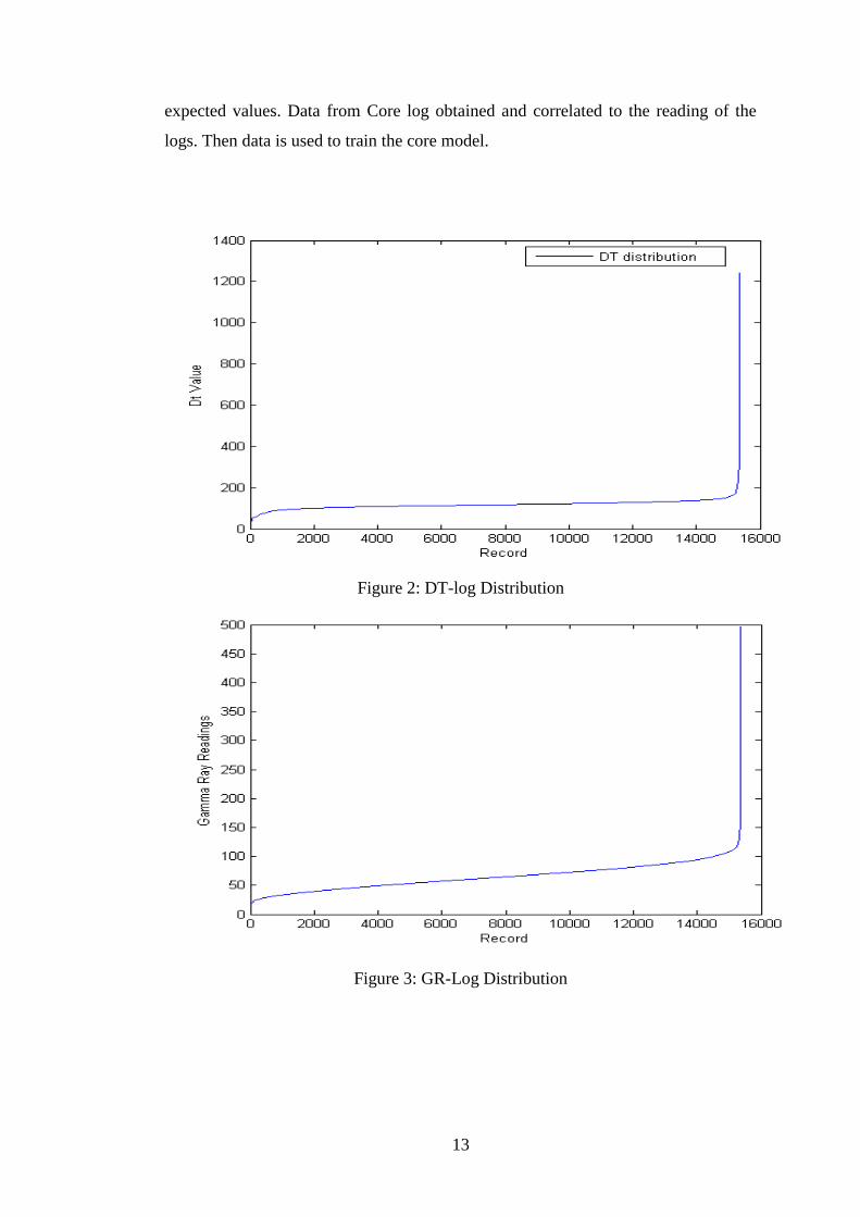
Total records of data obtained from Gullfaks is 333,220 line of data. The data is

organized so that for every parameter the network is trained over the whole range of

13

expected values. Data from Core log obtained and correlated to the reading of the

logs. Then data is used to train the core model.

Figure 2: DT-log Distribution

Figure 3: GR-Log Distribution

14

Figure 4: ILD-Log Distribution

Figure 5: ILM -Log Distribution

15

Figure 6: Nphi-Log Distribution

Figure 7: RHOB Distribution

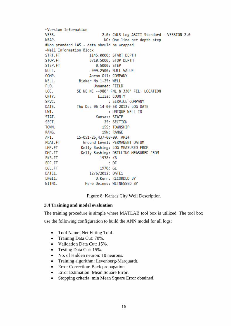
16

Figure 8: Kansas City Well Description

3.4 Training and model evaluation

The training procedure is simple where MATLAB tool box is utilized. The tool box

use the following configuration to build the ANN model for all logs:

Tool Name: Net Fitting Tool.

Training Data Cut: 70%.

Validation Data Cut: 15%.

Testing Data Cut: 15%.

No. of Hidden neuron: 10 neurons.

Training algorithm: Levenberg-Marquardt.

Error Correction: Back propagation.

Error Estimation: Mean Square Error.

Stopping criteria: min Mean Square Error obtained.

17

Steps for training the different models is illustrated in the figure below:



18



19



20

3.5 ANN Model Structure

Figure 14: ANN Model

The above figure represents the general structure for training model for logs &

porosity estimation. By using other logs, we can correlate the values of each log

which lead to another set of data of correlated logs which is combined to determine

the porosity values.

21

3.6 Training Different Models

Four models is developed to obtain best results in predicting the core data. Then

other 5 models is used to obtain the logs data.

3.6.1 Training Core Data

Table 1: LIST OF DIFFERENT MODEL TO BE TRAINED FOR CORE

Model -1- Direct Correlation between log Data and Core data without

changing input and outputs.

Model -2- First Model logs using logs ANN model then using their

outputs model ANN to predict the Porosity value.

Model -3- Normalize data from 1 to 0 then running log to porosity

model directly.

Model -4- Use a specific focused range for data ex. GR (20 – 200

API).

3.6.2 Training Log Data

Table 2: LIST OF DIFFERENT MODEL TO BE TRAINED FOR LOGS

Model -1- Sampling Rate of 1 record for every 100.



Model -4- Normalized log data from 0 to 1.

Model -5- Use a specific focused range for data

22

CHAPTER 4

RESULTS

4.1 Core Model Comparison

From the figure above as illustrated, we can see how the error distribution in each

model. Model-1- shows wide range of error from 0% to 25%, but the outliers

number are also considerably significant and with higher error between 25% and

Figure 15: Comparison between different models prediction (Error distribution

typing error at the graph captions)

23

50%. The model is indecisive, inaccurate and cannot be used to predict porosity from

log data. Model -2-‘s accuracyimproves on the outliers’ part as most of the data

within the control range but most error is still from 0% to 25% and average error is

almost 15% which is considered high. Model -3- is not viable at all as it range from

0% to 160% error evenly distributed across that range. Model -4- produces

satisfactory results where error is between 0% and 40%, where most probability of

error 3% to 18%. The mean error is 7%.

For low porosity, a 5% porosity reading with 18% error will give a shift in reading of

5.75% or 4.35% which is not highly significant. With high porosities, a 25% porosity

reading with 18% shift gives a reading of 29.5% or 21.5%.,which is considered

acceptable for high porosities values.

Figure 16: COMPARISON OF RANGE OF ERROR

The above figure shows the variation of error reading considering the highest value

of 18%. We can see that for the most important ranges of 10% to 20%. The effect of

error is considerably small and an acceptable result is obtained.

0

3

6

9

12

15

18

21

24

27

30

33

36

39

42

45

48

51

54

57

Illustration on boundries of prosity prediction model Error

porosity reading max boundry min boundry

porosity

reading

max

boundry

min

boundry

0 0 0

3 3.54 2.46

6 7.08 4.92

9 10.62 7.38

12 14.16 9.84

15 17.7 12.3

18 21.24 14.76

21 24.78 17.22

24 28.32 19.68

27 31.86 22.14

30 35.4 24.6

33 38.94 27.06

36 42.48 29.52

39 46.02 31.98

42 49.56 34.44

45 53.1 36.9

24

4.2 logs Model Comparison

DT prediction comparison between Model -3- and Model -5-.

Figure 17: Comparison between DT model -3- (top) and model -5-

(bottom) in Error distribution

25

GR prediction comparison between model -3- and model -5-

Figure 18: Comparison between NPHI model -3- (top) and model -5- (bottom) in Error

distribution

26

NPHI prediction comparison between model -3- and model -5-

Figure 19: Comparison between NPHI model -3- (top) and model -5-


27

ILD prediction comparison between Model -3- and Model -5-

Figure 20: Comparison between ILD model -3- (top) and model -5-


28

RHOB prediction comparison between Model -3- and Model -5-

Figure 21: Comparison between RHOB Model -3- (top) and Model -5-


29

ILM prediction comparison between Model -3- and Model -5-

Figure 22: Comparison between ILM Model -3- (top) and Model -5-


30

4.3 Trend logs prediction

Figure 25: Trend of DT prediction from Gullfaks field

31

Figure 24: Trend of GR prediction from Gullfaks field

Figure 25: Trend of ILD prediction from Gullfaks field

32

Figure 26: Trend of ILM prediction from Gullfaks field

Figure 27: Trend of NPHI prediction from Gullfaks field

33

Figure 28: DT Model prediction from Kansas City Data

34

Figure 29: GR Model prediction from Kansas City Data

Figure 30: ILD Model prediction from Kansas City Data

35

Figure 31: ILM Model prediction from Kansas City Data

Figure 32: NPHI Model prediction from Kansas City Data

36

4.4 Discussion of Findings

Based on the previous results obtained from different models shows the following

4.1.1 Ability of ANN model to predict reservoir porosity.

Once the model is trained on the reservoir data, ANN shows strong capability in

predicting different logs and petrophysical properties values. This returns to first that

in a single reservoir the heterogeneity model is considered constant and same

following specific function. The models generated represent a relation between the

reservoir physical and petrophysical properties. Ex. Different logs readings and

porosity readings.

4.1.2 Different training technique cause different results.

The models generated by ANN highly depend on method of training. More, it

depends on the true universal relation that exists between the input and targets.

On the other hand the model is as good as the training data is. Therefore we can

see the model accuracy increase from model (1), model (2) then model (4).model

(1) is constructed using all data record where they are simply divided randomly

then ran into training the model. That is the reason why the model shows high

number of outliers and errors outside the control box (not within boxplot diagram).

Model (2) is construct by predicting the porosity using two steps. First the

model predicting different logs reading from other readings, this lead to some

uncertainties correlation since we correlate each reading from original one. Then

those new correlated logs is inputted into a new model to directly predict porosity.

Model (4) go further to omit all obvious wrong readings such as reading porosity

of values more than 1. This leads to the optimum result. In reality further analysis

can be done on the data to improve its quality but that is outside the scope of this

study.

4.1.3 The model performance depend on the range where data is covered.

ANN models are highly sensitive to the actual readings numbers. For example, the

following set is considered good data for training,

37

{1, 2, 5, 6, 9, 2.3, 5.3}

On the other hand the following data is considered very confusing data for the model

training,

{1, 2, 5, 6, 9, 2.3, 5.3}

On the other hand the following data is considered very confusing data for the model

training:

{100, 0.1, 5, 4.6, 8333, 938}.

The second set is considered highly irregular and confusing for the training

method. This is observed in the ILM and ILD training, the model show very high

error and un capable of finding low error results even though it can predict the

trend in increasing or decreasing with the a good indication of the magnitude. A

solution is proposed by many scholars to normalize the data but that actually lead

to more error as observed in model (3).

4.1.4 ANN model has high speed training and testing capabilities.

A single ANN model can take between one tenth of a second to maximum of three

(3) min in training which is considered fast and reliable tool for training huge

number of small expert models. Within this research, 20 model can be created within

one (1) hour including organizing, training and testing data. Also ANN model

benefit from the fact that the testing computer consists of four cores which allow

ANN to utilize all four core in training and testing the data. That is due to the design

of ANN where each node can act as a single processing unit which allows it to

process simple task on very high speed to create a complex model at the end.

38

4.1.5 Other factor that affect training quality.

Other factors that can impact model quality and speed are as follows

1) Number of hidden layers

This factor actually highly depend on the complexity of

relation the model try to identify. The more hidden layers to

have the more complex the model will be which will impact

highly on the training time. A single hidden layer found to

be sufficient for most cases. Also in reservoir properties

identification a single layer found to be sufficient.

2) Transform function type

Transform function play essential role on how the final result is

passed to the next node. A tansig function is found to result

in high efficient model between inputs and hidden layer.

While for output it is more preferred to have a liner relation

of (Y= X).

3) Error Correction Algorithm.

There is a lot of different types of error correction algorithms

other than LM but LM model proved to be most used on

engineering related models and have higher accuracy than other

conventional error estimation methods. Testing other

algorithms is outside the scope of this research.

39

CHAPTER 5

CONCLUSIONS AND RECOMMENDATIONS

ANN models are highly flexible and can be used an many areas where it is

essential to have a mathematical model that can connect to variables that we cannot

final direct physical relation between them or the relation is too complex to be

formulated using normal mathematics.

However, obtaining the right model is method of trial and error and optimization

of input data. Trial and error in choosing optimum hidden neuron number which

highly depends on how many variables needed to define the mathematical

relationship. Also in using the optimum transfer function? This also complex of

what combination of those two variables? Finding the optimum model is a process

of large trial and error using all possible combinations. There is no exact way

to determine those two variables.

On the other hand, the quality of training data highly affects the final

mathematical model accuracy. Which impose a complexity on how certain are we

about our data obtained. And can we depend on it to obtain such mathematical

model. Data with high certainty only can be valid and used to train networks.

Up to date ANN have been used in many fields such as security systems and

monitoring systems, but the final decision is still decided and analyzed by human

eye before implementation. Which impose the question of applying ANN within

field. But definitely ANN can help in monitoring and assisting human decision.

ANN is mostly used in fields where huge data need to be analyzed or when

preliminary decision need to be taken on short notice with low risk margin.

Further recommendation will be to investigate the new types of ANN like

deep learning neural network where training process is more specific and easy to

control. Deep neural network can be trained to identify specific features for each

node which lead the overall learning accuracy increase and final model is more

expert.

Neural network also can be used to recognize different log drawing instead of

values. Where clustering and pattern recognition can perform better than normal

ANN method of comparing values to values. In such case the network will be

40

taught to identify curves and how to analysis them than analyzing data in

numerical form.

41

CHAPTER 6

References

Lo D. Mazzoni and S. venturini and sandro and C. Baio and M. Borghi, a. D. (2012,

January 1). Reducing Reservoir Uncertainties Using Advanced Wireline

Formation Testing. . Society of Petroleum Engineers. , doi:10.2118/154426-

MS.

A. kohlic, P. A. (10 January 2014). Application of Artificial Neural Networks for

Well Logs. International Petroleum Technology Conference, doi:

10.2523/17475-MS.

A. Kumar. ( 30 April 2012). Artificial Neural Network as a Tool for Reservoir

Characterization and its Application in the Petroleum Engineering. Offshore

Technology Conference., doi:10.4043/22967-MS.

Adams, S. J. (2005, January 1). Quantifying Petrophysical Uncertainties. Society of

Petroleum Engineers. , doi:10.2118/93125-MS.

Brock, J. (1986). Applied Open-Hole log Analysis. Houston, Texas: Gulf Publishing

Company.

Bronniman, G. S. (2014, October 14). Exploring Petrophysical Uncertainties Thanks

to Stochastic Well Log Data Interpretation: Termokarstovoye Field Case.

Society of Petroleum Engineers. , doi:10.2118/171211-MS.

J. K. Ali. (1994, January 1). Neural Networks: A New Tool for the Petroleum

Industry? . Society of Petroleum Engineers. , doi:10.2118/27561-MS.

Kumoluyi., A. O. (1994, January 1). Higher-Order Neural Networks in Petroleum

Engineering. . Society of Petroleum Engineers. , doi:10.2118/27905-MS.

M. Elshafei, G. M. (2009, January 1). Petrophysical Properties Determination of

Tight Gas Sands From NMR Data Using Artificial Neural Network. . Society

of Petroleum Engineers., doi:10.2118/118788-MS.

N. Al-Bulushi and M.Araujo and M. Kraaijveld and X. D Jing. (2007, January 1).

Predicting Water Saturation Using Artificial Neural Networks (ANNs).

Society of Petrophysicists and Well-Log Analysts.

42

P. Deo & D. C. Xue, &. F. (1 Januray 2009). Managing Uncertainty of Well Log

Data in Reservoir Characterization. Society of Petroleum Engineers. Society

of Petroleum Engineers, doi:10.2118/118980-MS.

P. S. Hegeman, a. C. (2009, February 1). Application of Artificial Neural Networks

to Downhole Fluid Analysis. Society of Petroleum Engineers. ,

doi:10.2118/123423-PA.

Shokir.., E.-M. (2004, January 1). Prediction of the Hydrocarbon Saturation in Low

Resistivity Formation via Artificial Neural Network. . Society of Petroleum

Engineers. , doi:10.2118/87001-MS.

T. M. Olson. (January 1998,). Porosity and Permeability Prediction in Low-

Permeability Gas Reservoirs From Well Logs Using Neura Networks.

Society of Petroleum Engineers., doi:10.2118/39964-MS.

Tinsley Oden, R. M. (November 2010). Computer Predictions with Quantified

Uncertainty. Part I. SIAM News, Volume 43, Number 9.

V. Berteig, a. K. (1988, January 1). Prediction of Hydrocarbon Pore Volume With

Uncertainties. Society of Petroleum Engineers, doi:10.2118/18325-MS.

Y. B Lind and A. R. Kabirova. (2014, October 14). Artificial Neural Networks in

Drilling Troubles Prediction. . Society of Petroleum Engineers. ,

doi:10.2118/171274-MS.

Y. Guo, Y. a. (1992, January 1). Artificial Intelligence I Neural Networks In

Geophysics. Society of Exploration Geophysicists.

1

CHAPTER 7

APPENDIX

APPENDIX – I – VBA code to extract data from .las files.

Sub organise()

rw1 = 73

cl1 = 1

rw2 = 1

cl2 = 1

Do While rw1 < 99999

Do While cl1 < 8

'MsgBox (rw1 & " " & cl1 & " " & rw2 & " " & cl2)

If Worksheets("1").Cells(rw1, cl1).Value = "" Then

GoTo nextcycle

End If

Worksheets("2").Cells(rw2, cl2).Value = Worksheets("1").Cells(rw1,

cl1).Value

cl2 = cl2 + 1

nextcycle:

If cl2 > 22 Then

rw2 = rw2 + 1

cl2 = 1

End If

cl1 = cl1 + 1

Loop

cl1 = 1

rw1 = rw1 + 1

Loop

End Sub

2

APPENDIX – II – VBA code to organise data from directory of .las files.

#include <fstream>

#include <iostream>

#include <string>

#include <stdio.h>

using namespace std;

int main()

{

string dir,name_file,txt;

int inpt[23];

int prnt[23];

ifstream filedir;

filedir.open("C:\\Users\\ahmed\\Desktop\\FYP_data\\b\\dir.txt");

while (filedir >> dir)

{ filedir >> name_file;

ifstream myfile;

myfile.open(dir);

int validme = 0, lenth = 0, mover = 0, allow = 0, lock1 = 0, lock2 = 0;

txt = "";

ofstream wrtin;

wrtin.open("C:\\Users\\ahmed\\Desktop\\FYP_data\\b\\data2\\" +

name_file);

while (myfile >> txt)

{ if (txt == "#" && validme < 1)

{ validme++;

lock1 = 1; }

if (txt == "DEPT" && validme < 2 && lock1 == 1)

{ validme++; }

if (txt == "~A")

{ validme = 3;

wrtin << endl;

allow = 1;

continue; }

if (validme == 2)

{ if (txt == "#")

{ continue; }

wrtin << txt << " ";

lenth++; }

if (allow == 1)

{ if (mover == lenth)

{ wrtin << endl;

mover = 0; }

if (txt == "#")

{ continue; }

wrtin << txt << " ";

mover++; }

//cout << txt<<endl; }

myfile.close();

wrtin.close(); }

getchar(); return 0; }

3

APPENDIX – III – C++ code to extract selective logs data from directory of .las

files.

#include <fstream>

#include <iostream>

#include <string>

#include <stdio.h>

#include <cmath>

#include <cstdlib>


int main()

{ cout << "start";

string dir, name_file, txt;

ifstream filedir; //open take directory of file

filedir.open("C:\\Users\\ahmed\\Desktop\\FYP_data\\b\\dir2.txt");


{ filedir >> name_file;

ifstream myfile;

myfile.open(dir);

txt = "";

ofstream wrtin;


name_file);

wrtin << name_file<<" ";

char a = txt[0];

int inpt[10] = { 0, 0, 0, 0, 0, 0, 0, 0, 0, 0 };

int b = 0, c = 0,allow = 0 ;

int max2 = 0, c1 = 0, max = 0, b1 = 0;


{

a = txt[0];

if (isdigit(a) && allow == 0)

{ allow = 1;

max2 = c; max = b;

wrtin << endl <<name_file<< " "; }

if ((txt == "DEPT" || txt == "DRHO" || txt == "DT" || txt == "GR" ||

txt == "CALI" || txt == "BS" || txt == "NPHI" || txt == "ILD" || txt == "ILM") && allow==0)

{ wrtin << txt<<" ";

inpt[b] = c;

b++; }

if (inpt[b1] == c1 && allow == 1)

{ wrtin << txt << " ";

b1++; }

if (!(b1 < max) && allow == 1)

{wrtin << endl<<name_file<<" ";

b1 = 0; }

if (allow == 0) { c++; }

if (allow == 1) { c1++; }

if (!(c1 < max2) && allow == 1)

{ c1 = 0; }

}

myfile.close();

wrtin.close(); }

getchar(); return 0;

}

4

APPENDIX – IV – C++ code to elimante logs without needed input data from

directory of .las files.

#include <fstream>

#include <iostream>

#include <string>

#include <stdio.h>

#include <cmath>

#include <cstdlib>


int main()

{ cout << "start"<<endl;

string dir, name_file, txt;

ifstream filedir; //open take directory of file

filedir.open("C:\\Users\\ahmed\\Desktop\\FYP_data\\b\\dir3.txt");


{ //filedir >> dir;

filedir >> name_file;

//cout <<"dir is: "<< dir << endl << "name_file is: "<<name_file << endl;

ifstream myfile;

myfile.open(dir);

txt = "";

char a = txt[0];

int counter = 0,skipper = 0;


{ a = txt[0];

//cout << "a is: " << a << endl;

//cout << txt << endl;

if (isdigit(a) && skipper == 1)

{ break; }

if (txt == name_file)

{ skipper = 1; }

if (txt == name_file || txt == "DEPT" || txt == "DRHO" || txt ==

"DT" || txt == "GR" || txt == "CALI" || txt == "BS" || txt == "NPHI" || txt == "ILD" || txt ==

"ILM")

{ counter++;

//cout << "counter1 is: "<<counter << endl;

//getchar(); }}

int allow = 0,count= 0;

ofstream wrtin;

if (counter > 10)

{ myfile.close();

myfile.open(dir);


name_file);

allow = 1; }

if (allow == 1)

{ while (myfile>>txt)

{ wrtin << txt << " ";

count++;

if (count >= counter)

{ wrtin << endl;

count = 0;}}} myfile.close(); wrtin.close(); }getchar();return 0;}

Documents

Improving Prediction of Wireline Data Using Artificial