Embed Size (px)
Citation preview
Improving Predictive Modeling in High Dimensional,Heterogeneous and Sparse Health Care Data
A THESIS
SUBMITTED TO THE FACULTY OF THE GRADUATE SCHOOL
OF THE UNIVERSITY OF MINNESOTA
BY
Chandrima Sarkar
IN PARTIAL FULFILLMENT OF THE REQUIREMENTS
FOR THE DEGREE OF
DOCTOR OF PHILOSOPHY
Jaideep Srivastava PhD , Sarah Cooley MD
August, 2015

c© Chandrima Sarkar 2015
ALL RIGHTS RESERVED

Acknowledgements
Firstly, I would like to express my sincere gratitude to my advisor Prof. Jaideep Srivas-
tava for the continuous support of my Ph.D study and related research, for his patience,
motivation, and immense knowledge. His guidance helped me in all the time of research
and writing of this thesis. I could not have imagined having a more suitable adviser
and mentor for my Ph.D study.
My sincere thanks also goes to my co-advisor Dr. Sarah Cooley, who provided me
an opportunity to work in her team as a research assistant, and who gave access to
valuable data and medical research information. Without her precious support it would
not be possible to conduct this research.
Besides my advisors, I would like to thank the rest of my thesis committee: Prof.Vipin
Kumar, Prof. Rui Kuang, and Dr. Prasanna Desikan, for their insightful comments and
encouragement, but also for the hard question which motivated me to widen my research
from various perspectives.
I recognize that this research would not have been possible without finance and
data resources. In this regard, I would like to thank Dr. Jeff S. Miller since the data
set used in this thesis was supported by National Institutes of Health/NCI grant P01
111412, PI Jeffrey S. Miller, M.D, utilizing the Masonic Cancer Center, University of
Minnesota Oncology Medical Informatics shared resource. I would also thank Allina
Health, for supporting me financially and by allowing application of some of my ideas
in their health care data during my tenure as a research assistant.
My sincere thanks also goes to Dr. Heather Britt, Tammie Lindquist and Tamara
Winden from Allina Health who helped he shape my interest and knowledge in the
domain of health scare. I also thank Dr. Tong Sun and Dr. Juan Li from PARC, a
Xerox company, who provided me an opportunity to join their team as intern, where I
i

learned interesting things with hands on experience in their laboratory.
I thank my fellow lab mates for the stimulating discussions, useful feed backs and
for all the fun we have had in the last four years. I would also thank all my close friends
from University of Minnesota for making this journey fun and light.
I would like to thank my mother Uma Sarkar who supported me spiritually through-
out writing my thesis and my life in general. I would also like to thank my sister Tuhina,
brother in law Shoubho, ma Sumita Roy and bapi Alok Roy, who were always support-
ing me and encouraging me with their best wishes. I thank my father Dipankar Sarkar
for his support during my childhood education that shaped my confidence to pursue
higher studies.
I would like to thank my husband Atanu Roy. He helped me immensely with tech-
nical support and insightful feed back to my ideas and was always there cheering me up
and stood by me through the good times and bad.
Most importantly, I thank the Supreme Divine Mother, who continues to make
impossible things possible.
ii

Dedication
I dedicate this thesis to my family.
iii
Abstract
In the past few decades predictive modeling has emerged as an important tool for
exploratory data analysis and decision making in health care. Predictive modeling is a
commonly used statistical and data mining technique that works by analyzing historical
and current data and generating a model to help predict future outcomes. It gives us
the power to discover hidden relationships in volumes of data and use those insights
to confidently predict the outcome of future events and interactions. In health care,
complex models can be created to combine patient information like demographic and
clinical information from care providers, in order to predict and improve model accuracy.
Predictive modeling in health care seeks out subtle data patterns to enhance decision
making such as care providers can recommend prescription drugs and services based on
patient profile.
Although all predictive techniques have different strengths and weaknesses, model
accuracy is mostly dependent on the raw input data with various features used to train
a predictive model. Model building often requires data pre-processing in order to reduce
the impact of the skewed property of the data or outliers. This helps by significantly
improving performance. From hundreds of available raw data fields, a subset is selected
and fields are pre-processed before being presented to a predictive modeling technique.
For example, there can be thousands of variables consisting of genetic, clinical and
demographic information for different groups of patients. Therefore detecting significant
variables for a particular group of patient can enhance model accuracy. Hence, the secret
behind a good predictive model often times depends on good pre-processing and more
so than the technique used to train the model.
While the above responsibilities of an effective and efficient data pre-processing
mechanism and its usage with predictive modeling in health care data are better un-
derstood, three key challenges were identified that faces this data pre-processing task.
These include,
1) High dimensionality: The challenge of high-dimensionality arises in diverse fields,
ranging from health care and computational biology to financial engineering and
iv

risk management. This work identifies that there is no single feature selection
strategy that is robust towards different families of classification or prediction
algorithm. The existing feature selection techniques produce different results with
different predictive models. This can be a problem when deciding about the best
predictive model to use while working with real high dimensional health care data
and especially without domain experts.
2) Heterogeneity in the data and data redundancy: Most of the real world data
is heterogeneous in nature, i.e. the population consists of overlapping homoge-
neous groups. In health care, Electronic Health Records (EHR) data consists of
diverse groups of patients with a wide range of diverse health conditions. This
thesis identifies that predictive modeling with a single learning model over hetero-
geneous data can result in inconclusive results and ineffective explanation of an
outcome. Therefore, it has been proposed in this thesis that, there is a need for
data segmentation/ co-clustering technique that extracts groups from data while
removing insignificant features and extraneous rows, giving result to an improved
predictive modeling with a learning model.
3) Data sparseness: When a row is created, storage is allocated for every column,
irrespective of whether a value exists for a given field. This gives rise to sparse
data which has a relatively high percentage of the variable’s cells, missing the
actual data. In health care, not all patients undergo every possible medical di-
agnostics and lab results are equally sparse. Such Sparse information or missing
values causes predictive models to produce inconclusive results. One primitive
technique is manual imputation of missing values by the domain experts. Today,
this scenario is almost impossible as the data is huge and high dimensional in na-
ture. A variety of statistical and machine learning based missing value estimation
techniques exist which estimates missing values by statistical analysis of the data
set available. However, most of these techniques do not consider the importance
of a domain expert’s opinion in estimating missing data. It has been proposed
in this thesis that techniques that use statistical information from the data as
well as opinion of the experts can estimate missing values more effectively. This
imputation procedure can results in non-sparse data which is closer to the ground
v

truth and that improves predictive modeling.
In this thesis, the following computational approaches has been proposed for han-
dling challenges described above for an effective and improved predictive modeling
1) For handling high-dimensional data a novel robust rank aggregation-based feature
selection technique has been developed using exclusive rank aggregation strategies
by Borda (1781) and Kemeny (1959). The concept of robustness of a feature
selection algorithm has been introduced, which can be defined as the property
that characterizes the stability of a ranked feature set toward achieving similar
classification accuracy across a wide range of classifiers. This concept has been
quantified with an evaluation measure namely, the robustness index (RI). The
concept of inter-rater agreement for improving the quality of the rank aggregation
approach for feature selection has also been proposed in this thesis.
2) The concept of a co-clustering has been proposed that is dedicated towards im-
proving predictive modeling. The novel idea of Learning based Co-Clustering
(LCC) has been developed as an optimization problem for a more effective and
improved predictive analysis. An important property of this algorithm is that
there is no need to specify the number of co-clusters. A separate model testing
framework has also been proposed in this work, for reducing model over-fitting
and for a more accurate result. The methodology has been evaluated on health
care data as a case study as well as several other publicly available data sets.
3) A missing value imputation technique based on domain expert’s knowledge and
statistical analysis of the available data has been proposed in this thesis. The
medical domain of HSCT has been chosen for the case study and the domain
expert’s knowledge is a group of stem cell transplant physician’s opinion. The
machine learning approach developed can be defined as - rule mining with expert
knowledge and similarity scoring based missing value imputation. This technique
has been developed and validated using real world medical data set. The results
demonstrate the effectiveness and utility of this technique in practice.
vi

Contents
Acknowledgements i
Dedication iii
Abstract iv
List of Tables x
List of Figures xiii
1 Introduction 1
1.1 Predictive Modeling In Health Care . . . . . . . . . . . . . . . . . . . . 1
1.2 Challenges Of Predictive Modeling . . . . . . . . . . . . . . . . . . . . . 5
1.3 Motivation . . . . . . . . . . . . . . . . . . . . . . . . . . . . . . . . . . 6
1.4 Contribution Of This Thesis . . . . . . . . . . . . . . . . . . . . . . . . . 6
1.4.1 Feature Selection For Dimensionality Reduction . . . . . . . . . . 6
1.4.2 Predictive Co-clustering For Data Heterogeneity and Dimension-
ality Reduction . . . . . . . . . . . . . . . . . . . . . . . . . . . . 7
1.4.3 Expert’s Knowledge Based Missing Value Estimation . . . . . . . 8
2 Feature Selection for High Dimensional data 9
2.1 Introduction . . . . . . . . . . . . . . . . . . . . . . . . . . . . . . . . . . 10
2.2 Methodology . . . . . . . . . . . . . . . . . . . . . . . . . . . . . . . . . 11
2.2.1 Rank Aggregation . . . . . . . . . . . . . . . . . . . . . . . . . . 12
2.2.2 Experimental Setup . . . . . . . . . . . . . . . . . . . . . . . . . 17
vii

2.2.3 Experimental Results and Discussion . . . . . . . . . . . . . . . . 21
2.2.4 Conclusion . . . . . . . . . . . . . . . . . . . . . . . . . . . . . . 26
2.3 Feature Selection in the Medical Domain: Improved Feature Selection
for Hematopoietic Cell Transplantation Outcome Prediction using Rank
Aggregation . . . . . . . . . . . . . . . . . . . . . . . . . . . . . . . . . . 27
2.3.1 Introduction . . . . . . . . . . . . . . . . . . . . . . . . . . . . . 28
2.3.2 Motivation and Related Work . . . . . . . . . . . . . . . . . . . . 31
2.3.3 Proposed Approach . . . . . . . . . . . . . . . . . . . . . . . . . 34
2.3.4 Details . . . . . . . . . . . . . . . . . . . . . . . . . . . . . . . . . 35
2.3.5 Data Set . . . . . . . . . . . . . . . . . . . . . . . . . . . . . . . . 37
2.3.6 Experimental Results . . . . . . . . . . . . . . . . . . . . . . . . 39
2.3.7 Conclusion . . . . . . . . . . . . . . . . . . . . . . . . . . . . . . 43
3 Predictive Overlapping Co-clustering for Heterogeneous data 45
3.1 Introduction . . . . . . . . . . . . . . . . . . . . . . . . . . . . . . . . . . 46
3.2 Related Work . . . . . . . . . . . . . . . . . . . . . . . . . . . . . . . . . 48
3.3 Problem Definition . . . . . . . . . . . . . . . . . . . . . . . . . . . . . . 51
3.4 An Intuition of the Proposed Approach . . . . . . . . . . . . . . . . . . 51
3.5 Learning Based Co-clustering Algorithm . . . . . . . . . . . . . . . . . . 52
3.5.1 Stopping Criteria . . . . . . . . . . . . . . . . . . . . . . . . . . . 58
3.5.2 Model Testing . . . . . . . . . . . . . . . . . . . . . . . . . . . . 59
3.5.3 Evaluation Metrics and Experimental Setup . . . . . . . . . . . . 61
3.5.4 Data Set . . . . . . . . . . . . . . . . . . . . . . . . . . . . . . . . 62
3.5.5 Results and Discussion . . . . . . . . . . . . . . . . . . . . . . . . 67
3.5.6 Conclusion . . . . . . . . . . . . . . . . . . . . . . . . . . . . . . 69
3.6 Co-clustering in Medical Domain: Improving prediction of Relapse in
Acute Myelogeneous Leukemia Patients with a Supervised Co-clustering
technique . . . . . . . . . . . . . . . . . . . . . . . . . . . . . . . . . . . 70
3.6.1 Introduction . . . . . . . . . . . . . . . . . . . . . . . . . . . . . 71
3.6.2 Related Work . . . . . . . . . . . . . . . . . . . . . . . . . . . . . 75
3.6.3 Supervised Co-clustering Algorithm . . . . . . . . . . . . . . . . 78
3.6.4 Experimental Evaluation . . . . . . . . . . . . . . . . . . . . . . 79
viii

3.6.5 Data set Properties . . . . . . . . . . . . . . . . . . . . . . . . . . 80
3.6.6 Results and Discussion . . . . . . . . . . . . . . . . . . . . . . . . 82
3.6.7 Conclusion . . . . . . . . . . . . . . . . . . . . . . . . . . . . . . 84
4 Knowledge based missing value imputation 85
4.1 Introduction . . . . . . . . . . . . . . . . . . . . . . . . . . . . . . . . . . 86
4.2 Related Work . . . . . . . . . . . . . . . . . . . . . . . . . . . . . . . . . 91
4.3 Problem Definition . . . . . . . . . . . . . . . . . . . . . . . . . . . . . . 93
4.4 Methodology . . . . . . . . . . . . . . . . . . . . . . . . . . . . . . . . . 94
4.4.1 Expert’s Knowledge Based Missing Value Imputation . . . . . . 94
4.4.2 Knowledge Collection From Experts . . . . . . . . . . . . . . . . 95
4.4.3 Integrating Knowledge With Rules . . . . . . . . . . . . . . . . . 97
4.4.4 Calculate Scores . . . . . . . . . . . . . . . . . . . . . . . . . . . 99
4.4.5 Using Scores For Data Imputation . . . . . . . . . . . . . . . . . 100
4.4.6 Evaluation Measures . . . . . . . . . . . . . . . . . . . . . . . . . 101
4.5 Result and Discussion . . . . . . . . . . . . . . . . . . . . . . . . . . . . 103
4.6 Conclusion . . . . . . . . . . . . . . . . . . . . . . . . . . . . . . . . . . 105
5 Conclusion and Discussion 107
References 111
ix

List of Tables
2.1 Rank Aggregation Algorithm . . . . . . . . . . . . . . . . . . . . . . . . 13
2.2 K step feature subset selection Algorithm . . . . . . . . . . . . . . . . . 15
2.3 Robustness Index calculation Algorithm . . . . . . . . . . . . . . . . . . 16
2.4 Data sets with attributes and instances . . . . . . . . . . . . . . . . . . 17
2.5 Results of paired ttest for Lung Cancer data set. IG- Information gain,
SU - Symmetric Uncertainty, CS- ChiSquare . . . . . . . . . . . . . . . . 18
2.6 Results of paired ttest for AML data set. IG- Information gain, SU -
Symmetric Uncertainty, CS- ChiSquare . . . . . . . . . . . . . . . . . . 18
2.7 Results of paired ttest for mfeat-fourier data set. IG- Information gain,
SU - Symmetric Uncertainty, CS- ChiSquare . . . . . . . . . . . . . . . . 18
2.8 Results of paired ttest for Embryonal Tumor data set. IG- Information
gain, SU - Symmetric Uncertainty, CS- ChiSquare . . . . . . . . . . . . 19
2.9 Results of paired ttest for Madelon data set. IG- Information gain, SU -
Symmetric Uncertainty, CS- ChiSquare . . . . . . . . . . . . . . . . . . 19
2.10 Results of paired ttest for Internet-Ads data set. IG- Information gain,
SU - Symmetric Uncertainty, CS- ChiSquare . . . . . . . . . . . . . . . . 19
2.11 Results of paired ttest for Leukemia-3c data set. IG- Information gain,
SU - Symmetric Uncertainty, CS- ChiSquare . . . . . . . . . . . . . . . . 20
2.12 Results of paired ttest for Arrhythmia data set. IG- Information gain,
SU - Symmetric Uncertainty, CS- ChiSquare . . . . . . . . . . . . . . . . 20
2.13 Classification algorithms used . . . . . . . . . . . . . . . . . . . . . . . . 20
2.14 Robustness Index with different data sets, IG- Information gain, SU -
Symmetric Uncertainty, CS- ChiSquare . . . . . . . . . . . . . . . . . . 23
x

2.15 Comparison of F-measure in different datasets using Naive Bayes Classi-
fier, IG- Information gain, SU - Symmetric Uncertainty, CS- ChiSquare 23
2.16 Comparison of F-measure in different datasets using J48 Decision Tree
Classifier, IG- Information gain, SU - Symmetric Uncertainty, CS- ChiSquare 24
2.17 Comparison of F-measure in different datasets using K Nearest Neigh-
bor Classifier, IG- Information gain, SU - Symmetric Uncertainty, CS-
ChiSquare . . . . . . . . . . . . . . . . . . . . . . . . . . . . . . . . . . . 24
2.18 Comparison of F-measure in different datasets using AdaBoost Classifier,
IG- Information gain, SU - Symmetric Uncertainty, CS- ChiSquare . . . 25
2.19 Comparison of F-measure in different datasets using Bagging Classifier,
IG- Information gain, SU - Symmetric Uncertainty, CS- ChiSquare . . . 25
2.20 Confirmation of Feature selection results with Multivariate analysis of
the data . . . . . . . . . . . . . . . . . . . . . . . . . . . . . . . . . . . . 41
3.1 Generate Co-clusters Algorithm . . . . . . . . . . . . . . . . . . . . . . . 57
3.2 Learning based co-clustering Algorithm . . . . . . . . . . . . . . . . . . 58
3.3 Calculate closest Co-Cluster . . . . . . . . . . . . . . . . . . . . . . . . . 60
3.4 Data Sets with Attributes and Instances . . . . . . . . . . . . . . . . . . 63
3.5 Madelon Data - Predictive Accuracy with Naive Bayes with initial num-
ber of k row and l column clusters and other parameters . . . . . . . . . 63
3.6 AML Data Predictive Accuracy with Naive Bayes with initial number of
k row and l column clusters and other parameters . . . . . . . . . . . . 63
3.7 MovieLens Data - Predictive Accuracy with Naive Bayes with initial num-
ber of k row and l column clusters and other parameters . . . . . . . . . 64
3.8 Internet Ads Data - Accuracy with Naive Bayes with initial number of k
row and l column clusters and other parameters . . . . . . . . . . . . . 64
3.9 AML Data - f-measure with J48 with initial number of k row and l column
clusters and other parameters . . . . . . . . . . . . . . . . . . . . . . . . 65
3.10 AML Data - f-measure with Naive Bayes with initial number of k row
and l column clusters and other parameters . . . . . . . . . . . . . . . . 65
3.11 Cluster precision comparison of LCC with BCC and SC. Parameters cor-
responsing to LCC for co-cluster generation, see figure 3.6, 3.5, 3.7 and
3.8 . . . . . . . . . . . . . . . . . . . . . . . . . . . . . . . . . . . . . . . 66
xi

3.12 Cluster Recall comparison of LCC with BCC and SC. Parameters cor-
responsing to LCC for co-cluster generation, see figure 3.6, 3.5, 3.7 and
3.8 . . . . . . . . . . . . . . . . . . . . . . . . . . . . . . . . . . . . . . . 66
3.13 Cluster F-measure comparison of LCC with BCC and SC. Parameters
corresponsing to LCC for co-cluster generation, see figure 3.6, 3.5, 3.7
and 3.8 . . . . . . . . . . . . . . . . . . . . . . . . . . . . . . . . . . . . 66
3.14 Notation Table . . . . . . . . . . . . . . . . . . . . . . . . . . . . . . . . 69
4.1 Missing value imputation Algorithm . . . . . . . . . . . . . . . . . . . . 101
xii

List of Figures
2.1 Flow diagram of the rank aggregation based feature selection alorithm. n
is the number of feature evaluation technique (using different statistical
properties of data). . . . . . . . . . . . . . . . . . . . . . . . . . . . . . 12
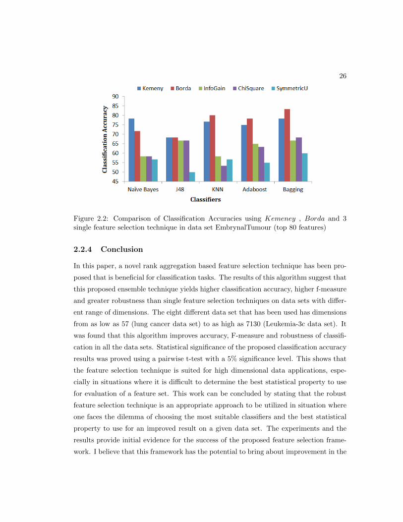
2.2 Comparison of Classification Accuracies using Kemeney , Borda and 3
single feature selection technique in data set EmbrynalTumour (top 80
features) . . . . . . . . . . . . . . . . . . . . . . . . . . . . . . . . . . . 26
2.3 Comparison of Classification Accuracies using Kemeney , Borda and
3 single feature selection technique in data set lung cancer data (top 8
features) . . . . . . . . . . . . . . . . . . . . . . . . . . . . . . . . . . . 27
2.4 Comparison of Classification Accuracies using Kemeney , Borda and 3
single feature selection technique in data set Internet-ads data (top 60
features) . . . . . . . . . . . . . . . . . . . . . . . . . . . . . . . . . . . 28
2.5 Comparison of Classification Accuracies using Kemeney , Borda and 3
single feature selection technique in data set mfeat-fourier data (top 9
features) . . . . . . . . . . . . . . . . . . . . . . . . . . . . . . . . . . . . 29
2.6 Comparison of Classification Accuracies using Kemeney , Borda and 3
single feature selection technique in data set Leukemia-3c data (top 60
features) . . . . . . . . . . . . . . . . . . . . . . . . . . . . . . . . . . . . 30
2.7 Comparison of Classification Accuracies using Kemeney , Borda and
3 single feature selection technique in data set Arrythmia data (top 36
features) . . . . . . . . . . . . . . . . . . . . . . . . . . . . . . . . . . . . 31
2.8 Comparison of Classification Accuracies using Kemeney , Borda and 3
single feature selection technique in data set AML data (top 25 features) 32
xiii
2.9 Comparison of Classification Accuracies using Kemeney , Borda and 3
single feature selection technique in data set Madelon data (top 40 feature) 33
2.10 Flow diagram of the entire process . . . . . . . . . . . . . . . . . . . . . 35
2.11 Classification Accuracy for treatment related mortality . . . . . . . . . 40
2.12 Classification Accuracy for Survival Rate . . . . . . . . . . . . . . . . . 41
2.13 Classifiecation Accuracy of Relapse Rate . . . . . . . . . . . . . . . . . 43
2.14 Classification Accuracy of Survival Rate for comparing rank aggregation
algorithm vs single feature selection algorithms . . . . . . . . . . . . . . 44
3.1 Flow diagram of the LCC algorithm . . . . . . . . . . . . . . . . . . . . 50
3.2 Student vs Subject scores . . . . . . . . . . . . . . . . . . . . . . . . . . 50
3.3 Intuitive proof of row column rearrangement result for co-cluster gener-
ation as given in algorithm 3.1 . . . . . . . . . . . . . . . . . . . . . . . 53
3.4 Various type of Data Segmentation process . . . . . . . . . . . . . . . . 54
3.5 Comparison with BCC and SC . . . . . . . . . . . . . . . . . . . . . . . 82
4.1 Example of incompleteness in datasets . . . . . . . . . . . . . . . . . . 89
4.2 Flow diagram of the expert’s knowledge based missing value imputation
technique. . . . . . . . . . . . . . . . . . . . . . . . . . . . . . . . . . . 96
4.3 Integrating knowledge into rules . . . . . . . . . . . . . . . . . . . . . . 98
4.4 Root Mean square error calculation for datasets with different sparseness
for different missing value estimation techniques. Lower the value it is
better . . . . . . . . . . . . . . . . . . . . . . . . . . . . . . . . . . . . . 103
4.5 Root Mean square error calculation for datasets with different sparseness
for different missing value estimation techniques. Lower the value it is
better . . . . . . . . . . . . . . . . . . . . . . . . . . . . . . . . . . . . . 104
4.6 Index of Agreement calculation for datasets with different sparseness for
different missing value estimation techniques. Higher the value it is better 105
4.7 Index of Agreement calculation for datasets with different sparseness for
different missing value estimation techniques. Higher the value it is better 106
5.1 Different techniques developed in this thesis in sequence . . . . . . . . . 109
xiv

Chapter 1
Introduction
1.1 Predictive Modeling In Health Care
Predictive modeling is a data modeling technique used in areas such as health care,
e-commerce, products, movie and music recommendation industries, bio-informatics ,
fraud detection and many others in order to model future behavior. Predictive modeling
can be also defined as the name given to a collection of techniques having in common
the goal of finding a relationship between a target, response, or ’dependent’ variable and
various predictor or ’independent’ variables. This is used to make inference regarding
values of the predictors and inserting them into a mathematical relationship in order to
make future predictions of the target variable of a new observation. These relationships
are never perfect in practice, and hence, it is often associated with some measure of
uncertainty for the predictions, typically a prediction interval with an assigned level of
confidence, for example 95%. The most important task in this process is the model
building. One common approach is to categorize the available predictor variables in to
three groups: 1) those unlikely to affect the response, 2) those almost certain to affect
the response and thus deemed significant in the predicting equation, and 3) those which
may or may not have an effect on the response. The challenge is to categorize and select
variables for predicting a given outcome.
Predictive modeling works by analyzing historical and current data and generating
a model to help predict future outcomes. In this process the data is first collected,
a statistical model is formulated, predictions are made, and the model is validated or
1
2
updated as additional data becomes available. For example, in risk modeling, various
member information is combined in complex ways during model building with demo-
graphic and lifestyle information from external sources to improve model accuracy. In
risk analysis models, past performance are analyzed to assess how likely a customer is
to exhibit a specific behavior in the future.This category also encompasses models that
seek out subtle data patterns to answer questions about customer performance, such as
fraud detection models. Similarly, in health care, patients information are combined to
asses how likely a patient will display a symptom or exhibit a certain outcome using
models built with various clinical and genetic information. Predictive models are built
depending on the situation that demands building a predictive model. For instance,
1) one might need to fit a well-defined parameterized model to the data, so a learn-
ing algorithm should be built which can find complex parameters on a large data set
without over-fitting. Another example can be 2) an algorithm with a ’black box’ view
is required. In other words one which can predict dependent variable as accurately as
possible. In this case a learning algorithm is needed which can automatically identify
the structure, interactions, and relationships in the data. One solution for case (1),
lasso and elastic-net regularized generalized linear models which are a set of modern
algorithms that are fast, work on huge data sets, and avoid over-fitting automatically
[1]. A probable solution for situation (2) is an ensembles of decision trees, namely;
’Random Forests’ which is an ensemble but efficient technique which has been the most
successful general-purpose algorithm in modern times [2] in many application areas.
There are two common types of predictive models namely, regression and classifi-
cation. Regression involves predicting a response with a certain degree of significance,
such as health measures related scores, quantity sold, housing price, or return on in-
vestment. Classification denotes prediction of a categorical response. For example, will
a leukemia patient survive the transplant given a specific donor ? which product brand
will be purchased and whether customers will buy the product or not ? Will the account
holder pay off or default on the loan? If a specific transaction is true or fraudulent?
Having information such as about a patients condition, particularly chronic condition(s)
is potentially useful for predicting risk. Since, a major part of predictive modeling in-
volves searching for useful predictors, these problems are defined by their dimension or
number of potential predictors and their number of observations in the data set. It is

3
the number of potential predictors in different domains that causes the most difficulty
in complex model building. There can be thousands of potential predictors with weak
relationships to the response. With the aid of computational techniques, hundreds or
thousands of models can be fit to subsets of the data and tested on newer observation of
the data thus evaluating each predictor. Therefore, in predictive modeling, finding good
subsets of predictors or explanatory variables forms an important part of the modeling
task. Models that fit the data well are better than models that fit the data poorly.
However, simple models are better than complex models since simple models do not
overfit the data. With the help of significantly useful predictors, many models can be
fitted to the available data, followed by evaluation of those models of their simplicity
and by how well they fit the data. In health care, extracted significant predictors can
benefit additionally by enhancing the decision making process. For example, signifi-
cant predictors extracted from acute myelogeneous leukemia data has been shown to
provide useful information for Hematopoietic Stem Cell Transplantation (HSCT) donor
selection process for leukemia patients [3].
Traditionally data models are built after specifying a theory for example, Bayesian
methods of statistical inference [4]. Popular methods, such as linear regression and lo-
gistic regression are used for estimating parameters for linear predictors. Model build-
ing involves fitting models to the available data. The fitted model is evaluated using
model diagnostics. Machine learning and data mining based predictive modeling in-
volves data-adaptive approach. This begins with analyzing the data to find useful
predictors. In this prior pre-processing stage and before the actual analysis theories
or hypotheses are given little importance. Data-adaptive methods are data-driven and
adapt to the available data and normally representing nonlinear relationships and in-
teractions among variables. The data determine the model. Another popular approach
is the model-dependent research which begins with the specification of a model and the
models are improved by comparing generated data with real data. This model is then
used to generate data, predictions, or recommendations. Some of the common examples
of model-dependent research are simulations and mathematical programming methods
and operations research tools [4].
In any modeling work, quantifying the uncertainty is one of the most important
task. For this purpose, traditional methods are useful namely, confidence intervals,
4
point estimates with associated standard errors, and significance tests. Measures such
as, probability intervals, prediction intervals, Bayes factors, subjective priors, and pos-
terior probability distributions can also be used. In order to judge one model against
another, measures such as Akaike information criterion (AIC) or the Bayes informa-
tion criterion (BIC) can be used. These measures helps to balance our model between
goodness-of-fit and providence. One of the most important part of predictive model-
ing is deciding on training-and-test data. A random splitting of a sample into training
and test sets could prove to be a draw of luck, especially when working with small
data sets. Hence, often certain statistical experiments can be conducted by execut-
ing a number of random splits and averaging performance measures from the resulting
test sets. A very useful approach is the k-fold cross-validation [5] which involves par-
titioning of the sample data into a number of folds of approximately equal size and
conducting a series of tests on the k splits. Another popular strategy is leave-one-out
cross-valuation, in which there are as many test sets as there are observations in the
sample. Training-and-test partition can also be conducted using a method commonly
known as bootstrap methods [6, 7]. The hypothesis in bootstapping is that if a sample
approximates the population from which it was drawn, then re-sampling from the previ-
ously drawn sample also approximates the population. A bootstrap procedure involves
repeated resampling with replacement. That is, many random samples are drawn with
replacement from the sample, and for each of these resamples, the statistic of interest
is calculated. Bootstrap method is interesting because it frees us from having to make
assumptions about the population distribution. In predictive modeling task such as
classification, commonly used evaluation measures are classification accuracy, precision,
recall or sensitivity, specificity and AUC. The purpose of these measures is to determine
the usefulness of our learned classifiers or of our learning algorithms on different data
sets.
Like any other modeling technique, predictive modeling especially in real world data,
frequently faces various challenges. These challenges usually arise from incomplete, het-
erogeneous, incorrect, or inconsistent data. In the next section, the primary challenges
and our motivation of this thesis has been described.
5
1.2 Challenges Of Predictive Modeling
In recent years, there has been a significant increase in data volume especially in the
health care domain. Data has become increasingly larger in both number of instances
and number of features in many real world applications. Some typical application areas
are genome projects [8], text categorization [9], customer relationship management [10],
image retrieval [11], social networks [12] and Healthcare [13]. The spectacular increase
in the amount of data is not only found in the number of samples collected for example
over time, but also in the number of attributes, or characteristics, that are simultane-
ously measured on a process. This enormity may cause serious problems in predictive
modeling with respect to scalability and learning performance of models. Two of the
major challenges in predictive modeling are high dimensional nature of the data and
sparseness. Data is often high dimensional in nature due to the enormous informa-
tion associated with each observation. However, the number of observation is limited
and the probability of possible information being associated with each observation is
low. This makes data high dimensional as well as sparse causing inference of accu-
rate data models difficult and complex. The difficulty in analyzing high-dimensional
data results from the conjunction of two effects. First, high-dimensional spaces have
geometrical properties that are counter-intuitive. Properties of higher dimensions can
not be observed or visually interpreted as the two-or three dimensional spaces. The
data analysis tools are most often designed based on intuitive properties of data in
low-dimensional spaces. These data analysis tools are best illustrated in two or three
dimensional spaces. In this regard, it is important to discuss the notion of ’curse of
dimensionality’ coined by Richard E. Bellman [14]. The curse of dimensionality refers
to the fact that complexity of many existing data mining algorithms is exponential with
respect to the number of dimensions. With increasing dimensionality, these algorithms
soon become computationally intractable which makes these algorithms inapplicable
in many real applications. Due to high dimension in data, the specificity of similari-
ties between points in a high dimensional space diminishes. [15] showed that, for any
point in a high dimensional space, the expected gap between the Euclidean distance to
the closest neighbor and that to the farthest point shrinks as the dimensionality grows.
Thus high dimensionality causes machine learning tasks (e.g., clustering) ineffective and

6
fragile because presence of noise diminishes accuracy of the model. Higher dimensions
also causes sparseness in the data which causes further decrease in the model accuracy.
Another important hurdle in the way of efficient predictive modeling is the presence of
hidden homogeneous overlapping groups in the data. This data heterogeneity makes a
predictive model similar to ’one size fits all’ concept, i.e. using same model for different
groups with different characteristics. This can render the predictive model less accurate
and far from the ground truth. An approximate solution to such problem is an effective
and efficient data segmentation technique that can extract these hidden groups for a
more accurate model building and enhanced effect of prediction outcome.
1.3 Motivation
It is now evident that handling high dimensional data is challenging as well important
for an effective and efficient predictive modeling. The focus of this work is to address
the issues of high dimensionality, data heterogeneity and data sparseness in the context
of predictive modeling. Over the recent years a variety of dimensionality reduction
methods and techniques for handling data sparseness have been proposed, to address
the challenges associated with predictive modeling.In this thesis, the above problems
has been explored in the context of predictive modeling in health care. In particular,
expert’s knowledge driven missing value imputation approaches has been considered. A
co-clustering based dimensionality reduction approache has been explored for improved
predictive modeling in heterogeneous data.
1.4 Contribution Of This Thesis
1.4.1 Feature Selection For Dimensionality Reduction
Feature selection is an essential step in successful data mining applications in the health
care domain, which can effectively reduce data dimensionality by removing the irrele-
vant (and the redundant) features. In the past few decades, researchers have developed
large number of feature selection algorithms. These algorithms are designed to serve
different purposes, are of different models, and all have their own advantages and disad-
vantages. These algorithm use various different statistical measures to evaluate features.
7
In this thesis, several different feature selection techniques has been examined and a rank
aggregation based feature selection technique has been developed that aggregates the
consensus properties of various feature selection methods to develop a more optimal
solution. The ensemble nature of our technique makes it more robust across various
classifiers. In other words, it is stable towards achieving similar and ideally higher
classification accuracy across a wide variety of classifiers. The concept of robustness
has been quantified with a measure known as the Robustness Index (RI). An extensive
empirical evaluation of our technique has been performed on health care domain as well
as seven other data sets with different dimensions including Arrythmia, Lung Cancer,
Madelon, mfeat-fourier, internet-ads, Leukemia-3c and Embryonal Tumor and a real
world data set namely Acute Myeloid Leukemia (AML). It has been demonstrate not
only that our algorithm is more robust, but also that compared to other techniques our
algorithm improves the classification accuracy by approximately 3-4% (in data set with
less than 500 features) and by more than 5% (in data set with more than 500 features),
across a wide range of classifiers.
1.4.2 Predictive Co-clustering For Data Heterogeneity and Dimen-
sionality Reduction
Hidden homogeneous blocks of data commonly referred as co-clusters [16] has been
found to provide significant advantages to several application domains. This is because,
in real world problems, the presence of insignificant features and extraneous data can
greatly limit the accuracy of learning models built on the data. Therefore, instead
of building predictive models on data from a noisy domain, homogeneous groups can
be extracted from the data for building more effective predictive models. This can
find application in several domain including targeted marketing and recommendation.
Motivated by this, in this thesis a novel co-clustering algorithm has been presented
called Learning based co-clustering (LCC). The key idea of our algorithm is to generate
optimal co-clusters by maximizing predictive power of the co-clusters subject to the
constraints on the number of co-clusters. The resulting clusters are high in predictive
power (for example classification accuracy, f-measure) when a learning (classification)
model is built on them.

8
1.4.3 Expert’s Knowledge Based Missing Value Estimation
In this thesis, a missing value imputation technique has been developed that is based on
expert’s knowledge and statistical analysis of the available data. The medical domain of
HSCT has been chosen for analysis and case study and a group of stem cell transplant
physician’s opinion has been considered as the domain expert’s knowledge. The machine
learning approach developed can be defined as - Expert Knowledge based Missing Value
Imputation (EKMVI). EKMVI techniques has been developed and findings has been
validate with real world AML data set. The results demonstrate the effectiveness and
utility of our techniques in practice in the domain of health care.

Chapter 2
Feature Selection for High
Dimensional data
Although feature selection is a well-developed research area, there is an ongoing need to
develop methods to make classification task more efficient. One important challenge is
the lack of a universal feature selection technique which produces similar outcomes with
all types of classifiers. This is because all feature selection techniques have individual
statistical biases while classifiers exploit different statistical properties of data for evalu-
ation. In numerous situations this can put researchers into dilemma as to which feature
selection method and a classifiers to choose from a vast range of choices. In this re-
search, a technique that aggregates the consensus properties of various feature selection
methods to develop a more optimal solution has been proposed. The ensemble nature of
this proposed technique makes it more robust across various classifiers. In other words,
it is stable towards achieving similar and ideally higher classification accuracy across a
wide variety of classifiers. This concept of robustness has been quantified as a measure
known as the Robustness Index (RI). An extensive empirical evaluation of this technique
has been performed, on eight data sets with different dimensions including Arrythmia,
Lung Cancer, Madelon, mfeat-fourier, internet-ads, Leukemia-3c and Embryonal Tumor
and a real world data set namely acute myeloid leukemia (AML). This research not only
demonstrate that this proposed algorithm is more robust, but also that compared to
other techniques this algorithm improves the classification accuracy by approximately
9

10
3-4% (in data set with less than 500 features) and by more than 5% (in data set with
more than 500 features), across a wide range of classifiers.
2.1 Introduction
We live in an age of exploding information where accumulating and storing data is easy
and inexpensive. In 1991 it was pointed out that the amount of stored information
doubles every twenty months [17]. Unfortunately, the ability to understand and utilize
this information does not keep pace with its growth. Machine learning provide tools
by which large quantities of data can be automatically analyzed. Feature selection
is one of the fundamental steps of machine learning. Feature selection identifies the
most salient features for learning and focuses a learning algorithm on those properties
of the data that are most useful for analysis and future prediction. It has immense
potential to enhance knowledge discovery by extracting useful information from high
dimensional data as shown in previous studies in various important areas [18, 19, 20, 9].
In this work, I propose to develop an improved rank aggregation based feature selection
method which will produce a feature set that is robust across a wide range of classifiers
than the traditional feature selection techniques. In this work [3] we developed the
idea of rank aggregation based feature selection approach and we showed that feature
selection for supervised classification tasks can be accomplished on the basis of ensemble
of various statistical properties of data. In this work, the idea has been extended by
developing the rank aggregation based feature selection algorithm with exclusive rank
aggregation approaches such as Kemeny [21] and Borda [22]. The algorithm has been
evaluated using five different classifiers over eight data set with varying dimensions.
Feature selection techniques can be classified into filter and wrapper approaches
[23, 24]. In this paper, I focus on Filter Feature Selection because it is faster and
more scalable [20]. Feature selection techniques using distinct statistical properties of
data have some drawbacks; for example information gain is biased towards choosing
attributes with a large number of values and Chi square is sensitive to sample size. This
indicates a statistical bias towards achieving the most optimal solution for classification
problem. In other words, there will be a variation in classification performance due
to the partial ordering imposed by the evaluation measures (for example information

11
gain and chis square statistics) over the space of hypotheses [25]. It has been shown
that ensemble approaches reduces the risk of choosing a wrong hypothesis from many
existing hypothesis in the solution space [26]. Ensemble technique has also been used in
various applications showing notable improvement in the results such as [27, 28, 29, 30].
To the best of my knowledge, no other study has focused on an extensive performance
evaluation of rank aggregation based feature selection technique using exclusive rank
aggregation strategies such as Kemeny [21].
To summarize, this work has the following contributions:
1) Development of a novel rank aggregation based feature selection technique using
exclusive rank aggregation strategies namely Borda [22] and Kemeny [21].
2) Extensive performance evaluation of the rank aggregation based feature selection
method using five different classification algorithms over eight data set of varying
dimensions. Pairwise statistical tests were performed with 5% significance level
to prove the statistical significance of the classification accuracy results.
3) The concept of robustness was introduced as Robustness Index (RI) of a feature
selection algorithm. RI can be defined as the property which characterizes the
stability of a ranked feature set towards achieving similar classification accuracy
across a wide range of classifiers.
4) The concept of inter-rater agreement has been proposed for improving the quality
of rank aggregation approach for feature selection.
The remainder of the paper is organized as follows. Section 2 is the methodology.
Section 3 describes the experimental results and discussion. In section 4, conclusion
has been presented. *In this work the terms variables, features and attributes has been
used with the same meaning.
2.2 Methodology
The process of rank aggregation based feature selection technique consists of the fol-
lowing steps: A non-ranked feature set is evaluated with n feature selection/evaluation
techniques. This gives rise to n sets of ranked feature sets which differ in their rank
12
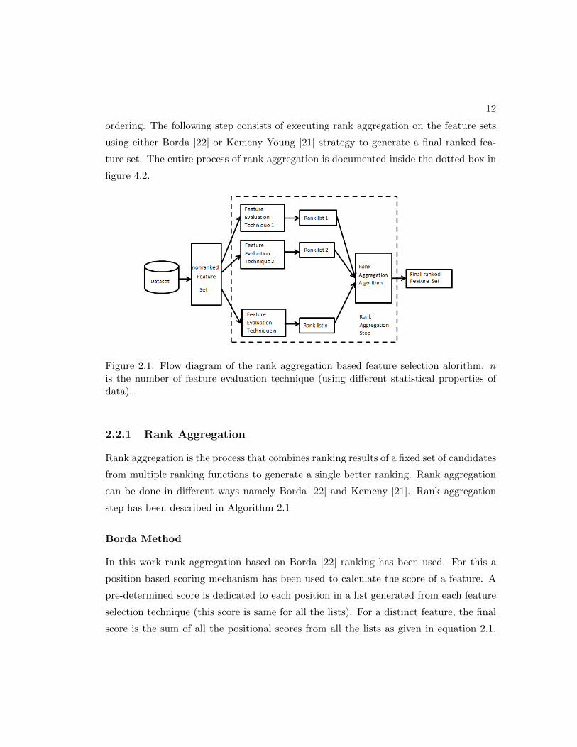
ordering. The following step consists of executing rank aggregation on the feature sets
using either Borda [22] or Kemeny Young [21] strategy to generate a final ranked fea-
ture set. The entire process of rank aggregation is documented inside the dotted box in
figure 4.2.
Figure 2.1: Flow diagram of the rank aggregation based feature selection alorithm. nis the number of feature evaluation technique (using different statistical properties ofdata).
2.2.1 Rank Aggregation
Rank aggregation is the process that combines ranking results of a fixed set of candidates
from multiple ranking functions to generate a single better ranking. Rank aggregation
can be done in different ways namely Borda [22] and Kemeny [21]. Rank aggregation
step has been described in Algorithm 2.1
Borda Method
In this work rank aggregation based on Borda [22] ranking has been used. For this a
position based scoring mechanism has been used to calculate the score of a feature. A
pre-determined score is dedicated to each position in a list generated from each feature
selection technique (this score is same for all the lists). For a distinct feature, the final
score is the sum of all the positional scores from all the lists as given in equation 2.1.
13
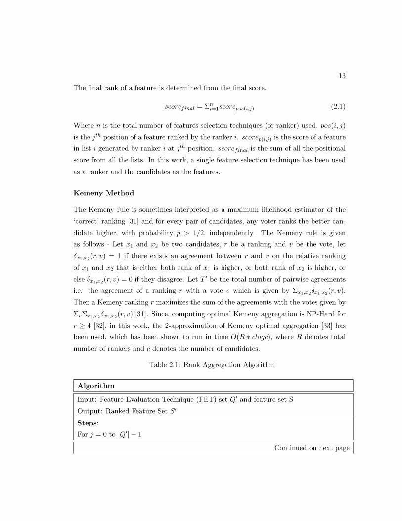
The final rank of a feature is determined from the final score.
scorefinal = Σni=1scorepos(i,j) (2.1)
Where n is the total number of features selection techniques (or ranker) used. pos(i, j)
is the jth position of a feature ranked by the ranker i. scorep(i,j) is the score of a feature
in list i generated by ranker i at jth position. scorefinal is the sum of all the positional
score from all the lists. In this work, a single feature selection technique has been used
as a ranker and the candidates as the features.
Kemeny Method
The Kemeny rule is sometimes interpreted as a maximum likelihood estimator of the
‘correct’ ranking [31] and for every pair of candidates, any voter ranks the better can-
didate higher, with probability p > 1/2, independently. The Kemeny rule is given
as follows - Let x1 and x2 be two candidates, r be a ranking and v be the vote, let
δx1,x2(r, v) = 1 if there exists an agreement between r and v on the relative ranking
of x1 and x2 that is either both rank of x1 is higher, or both rank of x2 is higher, or
else δx1,x2(r, v) = 0 if they disagree. Let T ′ be the total number of pairwise agreements
i.e. the agreement of a ranking r with a vote v which is given by Σx1,x2δx1,x2(r, v).
Then a Kemeny ranking r maximizes the sum of the agreements with the votes given by
ΣvΣx1,x2δx1,x2(r, v) [31]. Since, computing optimal Kemeny aggregation is NP-Hard for
r ≥ 4 [32], in this work, the 2-approximation of Kemeny optimal aggregation [33] has
been used, which has been shown to run in time O(R ∗ clogc), where R denotes total
number of rankers and c denotes the number of candidates.
Table 2.1: Rank Aggregation Algorithm
Algorithm
Input: Feature Evaluation Technique (FET) set Q′ and feature set S
Output: Ranked Feature Set S′
Steps:
For j = 0 to |Q′| − 1
Continued on next page

14
Table 2.1 – continued from previous page
S′′ = S, where S′′ is a temporary variable
Rank S′′ using FETj where FETj ∈ Q′
add S′′ to list L
S′=aggregated feature set from L using equation 2.1
Analysis of Rankers with Inter Rater Agreement
Inter Rater Agreement (IRA) can be used as a pre-processing step prior to the rank
aggregation step. The main motivation for this step is the analysis of the homogeneity or
consensus among the rank ordering generated by each ranker. Each ranker uses different
measures for evaluating the candidates and hence generates a different rank ordering.
There can be possibility that the rank ordering generated by one of the ranker is highly
inconsistent with the other rankers. This might cause the final aggregated rank ordering
to be far away from the ground truth (optimal) ordering. In this paper, the assumption
that rank ordering which is in consensus with the majority of the rankers are closest
to the ground truth, has been made. Hence, for improving the rank ordering generated
by the ranker, the concept of Inter-Rater Agreement (IRA) has been proposed which
analyses the degree of agreement among rankers. An Intraclass Correlation (ICC)[34]
approach has been used for calculating IRA. The ICC assesses rating reliability by
comparing the variability of different ratings of the same subject to the total variation
across all ratings and all subjects, as formulated in Equation 2.2.
ICC =V (b)2
(V (w)2 + V (b)2)(2.2)
where V (w)2 is the pooled variance within subjects, and V (b)2 is the variance of the
trait between subjects. The IRA lies between 0 to 1 where 0 is the least reliable rating
and 1 is the most reliable rating for a group of rankers. A heuristically determined
threshold T has been used, which is for eliminating rankers who tends to disrupts the
homogeneity in ranking from the group of rankers.

15
K-step feature subset Selection
The K-step feature subset selection is a post processing step to the rank aggregation
step with a focus on generating a feature subset from the final rank aggregated feature
set. In this process, firstly, for each classification algorithm, the classification accuracy
has been determined, of each top i feature subset where 1 ≤ i ≤ k where k is the total
number of features in the feature subset. Next, the feature subset with the maximum
classification accuracy across all the classification algorithms has been used, as the final
feature subset as given in Algorithm 2.2.
Table 2.2: K step feature subset selection Algorithm
Algorithm
Input: Feature Set S′, Dataset D, Classifiers set M
Output: feature subset of size k
Steps:
1. set S∗ ⊂ S′, mt ∈M and Σt|mt| = |M | and Kj ∈ S′ with K1 < K2..Kj .. < Kk where
K is the feature subset, 1 > j > k
2. For1 < i < |M |3. For1 < j < K
4. add feature set Kj to S∗
5. learn S∗ using Mi
6. Calculate accuracy of Mi and store it in list tempj
7. EndFor
8. search tempj for 1 < j < K with the highest predictive power for Mi and store in
K∗i9. EndFor
10. select the MAX(K∗i) where 1 < i < |M |
Evaluation Measure
This algorithm has been evaluated based on three evaluation measures as discussed
below -

16
1 Classification accuracy - accuracy is calculated as the percentage of correctly clas-
sified instances by a given classifier. At first a feature subset of size K using a
K-step feature subset selection approach as described in the previous section has
been obtained. Classification accuracy of this feature subset was determined and
recorded using five different classifiers for evaluation purpose.
2 F-measure - Weighted (by class size) average F-measure was obtained from the
classification using feature subset with the same five classifiers as above.
3 Robustness Index (RI) - Robustness can be defined as the property that char-
acterizes the stability of a feature subset towards achieving similar classification
accuracy across a wide range of classifiers. In order to quantify this concept a
measure called robustness index (RI) has been introduced, which can be utilized
for evaluating the robustness of a feature selection algorithm across a variety of
classifiers. Intuitively, RI measures the consistency with which a feature subset
generates similar (ideally higher) classification accuracy (or lower classification
error) across a variety of classification algorithms when compared with feature
subsets generated using other methods. The step-by-step process of robustness
index is described in algorithm 2.3
Table 2.3: Robustness Index calculation Algorithm
Algorithm
Input: Classification models Mi , where 1 ≤ i ≤ m , m is the number of classifiers used,
Feature set fk generated from p feature selection techniques, where k is number of top
features
Output: Robustness Index rp, for each p feature selection technique
Steps:
1. Fori = 0 to m− 1 ; For each Mi
2. Forj = 0 to p− 1
3. Cp = classification error with fk
5. EndFor
6. Rank each p based on Cp score and save
Continued on next page

17
Table 2.3 – continued from previous page
7. EndFor
8. Fori = 0 to p− 1
9. Aggregate the ranks across Mi for 1 < i < m using equation 2.1
10. Assign rp = aggregated ranks
11. EndFor
The motivation behind the concept of robustness is as follows: it is not an easy task
to determine the best classifier to use for a classification task prior to actually using that
model. A robust technique helps one to choose a classification model with the minimum
risk in choosing an inappropriate model.
2.2.2 Experimental Setup
Data Set
Eight different types of data set shown in Table 3.4 has been used. Acute myeloid
leukemia or AML is a real world data set that contains 69 demographic, genetic, and
clinical variables from 927 patients who received myeloablative, T-cell replete, unrelated
donor (URD) stem cell transplants [3]. Data sets includes Embryonal Tumours of the
Central Nervous System [35], madelon and Internet-ads [36], Leukemia-3c , Arrythmia,
Lung Cancer and mfeat-fourier [37] from UCI KDD as listed in Table 3.4.
Table 2.4: Data sets with attributes and instances
Data set Attributes Instances
Lung Cancer 57 32
AML 69 927
Mfeat-fourier 77 2000
Arrhythmia 280 452
Madelon 501 2600
Internet-Ads 1559 3279
Continued on next page
18
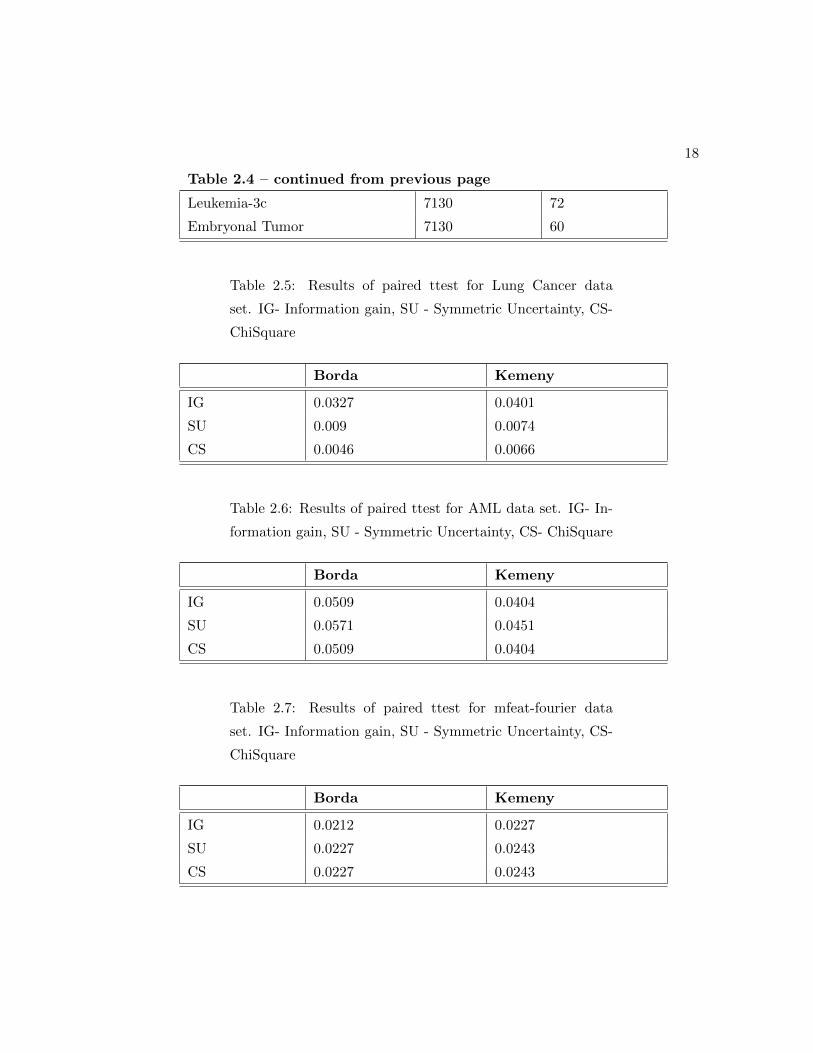
Table 2.4 – continued from previous page
Leukemia-3c 7130 72
Embryonal Tumor 7130 60
Table 2.5: Results of paired ttest for Lung Cancer data
set. IG- Information gain, SU - Symmetric Uncertainty, CS-
ChiSquare
Borda Kemeny
IG 0.0327 0.0401
SU 0.009 0.0074
CS 0.0046 0.0066
Table 2.6: Results of paired ttest for AML data set. IG- In-
formation gain, SU - Symmetric Uncertainty, CS- ChiSquare
Borda Kemeny
IG 0.0509 0.0404
SU 0.0571 0.0451
CS 0.0509 0.0404
Table 2.7: Results of paired ttest for mfeat-fourier data
set. IG- Information gain, SU - Symmetric Uncertainty, CS-
ChiSquare
Borda Kemeny
IG 0.0212 0.0227
SU 0.0227 0.0243
CS 0.0227 0.0243

19
Table 2.8: Results of paired ttest for Embryonal Tumor data
set. IG- Information gain, SU - Symmetric Uncertainty, CS-
ChiSquare
Borda Kemeny
IG 0.0155 0.0197
SU 2.7E-04 6.0E-06
CS 0.0225 0.0255
Table 2.9: Results of paired ttest for Madelon data set.
IG- Information gain, SU - Symmetric Uncertainty, CS-
ChiSquare
Borda Kemeny
IG 0.0164 0.0164
SU 0.0139 0.0139
CS 0.0164 0.0164
Table 2.10: Results of paired ttest for Internet-Ads data
set. IG- Information gain, SU - Symmetric Uncertainty, CS-
ChiSquare
Borda Kemeny
IG 0.0119 0.0119
SU 0.0119 0.0119
CS 0.0119 0.0119

20
Table 2.11: Results of paired ttest for Leukemia-3c data
set. IG- Information gain, SU - Symmetric Uncertainty, CS-
ChiSquare
Borda Kemeny
IG 0.0015 0.0015
SU 5.3E-04 5.3E-04
CS 3.8E-04 3.8E-04
Table 2.12: Results of paired ttest for Arrhythmia data
set. IG- Information gain, SU - Symmetric Uncertainty, CS-
ChiSquare
Borda Kemeny
IG 0.0157 0.0283
SU 0.0049 0.013
CS 0.0034 0.0084
Table 2.13: Classification algorithms used
Classifiers Settings
Naive Bayes estimator classes
J48 pruned C4.5 decision tree
KNN k=3; brute force search algorithm; Euclidean distance function
AdaboostM1 base classifier: Decision Stump,10 boost iterations, % of weight mass
for training was 100
Bagging weak classifier: fast decision tree learner, bag size as 100% , 10 bagging
iterations

21
Statistical Test of Significance
Pairwise t-test with a 5% significance level has been performed, in order to measure the
statistical significance of the classification accuracy result. The null hypothesis is that
the difference between classification accuracy result obtained from the two algorithms
considered in the pairwise test, comes from a normal distribution with mean equal to
zero and unknown variance. The null hypothesis has been rejected, if p − value is less
than 5% significance level. The results are given in Tables 2.6, 2.12, 2.8, 2.10, 2.11, 2.5,
2.9 and 2.7.
2.2.3 Experimental Results and Discussion
The performance of the proposed feature selection algorithm has been evaluated in terms
of classification accuracy, F-measure and robustness by comparing with three feature se-
lection techniques namely information gain attribute evaluation, symmetric uncertainty
attribute evaluation and chi square attribute evaluation[38]. A feature selection tech-
niques has been used with the help of IRA method assuming an IRA threshold of 0.75
(heuristically determined). This rank aggregation based feature selection algorithm has
been referred as Kemeny and Borda (using Kemeny and Borda method respectively)
in the figures shown in this paper.
The results of classification accuracy over eight data sets are given in figures 2.8,
2.2, 2.6, 2.7, 2.4, 2.3, 2.9 and 2.5. Using Algorithm 2.1 and 2.2 feature subsets has been
generated, for each data set indicated in a bracket in the tables 2.14 and 2.18, 2.19, 2.16,
2.15 and 2.17 . Next, classification has been performed using five different classifiers
shown in figure 2.2, 2.3, 2.4, 2.5, 2.6, 2.7, 2.8, 2.9. Figures 2.2, 2.4 2.9 and 2.6 shows
classification accuracy for data sets with over 500 variables. In these four data sets, the
accuracy with Kemeny and Borda is more than 5% higher as compared to those with
the three single feature selection methods. In the four other data sets shown in figure
2.3, 2.5, 2.7 and 2.8, the classification accuracy is higher by approximately 3-4 % across
all the classifiers.
Next, pairwise statistical significance test has been performed with a 5% significance
level to prove the statistical significance of the accuracy results. The p − values has
been calculated for every data set, comparing Kemeny and Borda with three feature

22
selection techniques as depicted in Tables 2.6, 2.12, 2.8, 2.10, 2.11, 2.5, 2.9 and 2.7 .
Table 2.14 shows the comparison of robustness index as calculated using Algorithm
2.3. Lower the value of RI, more robust is the technique, i.e. Robustness index equals
1 is more robust than an RI equals 3. Table 2.14 shows that both Kemeny and Borda
has robustness index of either 1 or 2 with every data set. This shows that Kemeny
and Borda are more robust than the other traditional feature selection techniques. The
motivation behind this analysis is that, when one is unable to decide on the best classi-
fication algorithm to use on a given data set, the proposed feature selection algorithm
will help with a technique that will ensure a lower classification error over a variety of
classification algorithms. The number in parentheses beside the data set names in Table
2.14 indicates the size of the feature subset.
In tables 2.18, 2.19, 2.16, 2.15 and 2.17, weighted (by class size) average F-measures
(defined as the harmonic means of precision and recall) has been calculated, generated
using Kemeny and Borda with three feature selection methods using five different
classifiers as given in Table 2.13. The number in parentheses beside the data set names
in every figure indicates the size of the feature subset used for classification. It can be
seen that F-measure with Kemeny and Borda is higher in almost all the cases. This
shows that apart from accuracy, the sensitivity and specificity generated with different
classifiers using the proposed rank aggregation based feature selection method can be
improved.
The results of these analysis show that this rank aggregation based feature selection
algorithm is an efficient technique suited for various kinds of data sets including the
ones with features greater than 1000. The proposed method gives a higher classification
accuracy, f-measure and greater robustness than the other traditional methods over a
wide range of classifiers. This method is advantageous especially in cases where it is
difficult to determine the best statistical property for evaluation of a given data set. The
greatest advantage in having a robust technique is that, there will be fewer dilemmas
in deciding on the most appropriate classifier to use from the vast range of choices.

23
Table 2.14: Robustness Index with different data sets, IG- In-
formation gain, SU - Symmetric Uncertainty, CS- ChiSquare
Data Sets Kemeny Borda IG SU CS
AML (25) 1 1 3 2 3
Lung Cancer (8) 2 1 3 3 4
Arrhythmia (36) 1 2 4 5 3
mfeat-fourier (9) 2 1 4 3 3
madelon (40) 1 1 2 3 2
Internet-Ads (60) 1 1 2 2 2
Leukemia-3c (60) 1 1 2 3 3
Embyonal Tumor (60) 2 1 3 4 5
Table 2.15: Comparison of F-measure in different datasets
using Naive Bayes Classifier, IG- Information gain, SU - Sym-
metric Uncertainty, CS- ChiSquare
Data Sets Kemeny Borda IG SU CS
AML (25) 0.67 0.67 0.64 0.65 0.64
mfeat-fourier (9) 0.79 0.79 0.77 0.77 0.77
Arrhythmia (36) 0.67 0.67 0.53 0.56 0.54
madelon (40) 0.60 0.60 0.53 0.53 0.53
Internet-Ads (60 0.95 0.95 0.94 0.94 0.94
Leukemia-3c (60) 0.99 0.99 0.81 0.73 0.79
Embyonal Tumor (60) 0.74 0.72 0.62 0.59 0.61
Lung Cancer (8) 0.45 0.45 0.46 0.51 0.40
24
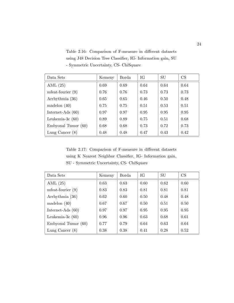
Table 2.16: Comparison of F-measure in different datasets
using J48 Decision Tree Classifier, IG- Information gain, SU
- Symmetric Uncertainty, CS- ChiSquare
Data Sets Kemeny Borda IG SU CS
AML (25) 0.69 0.69 0.64 0.64 0.64
mfeat-fourier (9) 0.76 0.76 0.73 0.73 0.73
Arrhythmia (36) 0.65 0.65 0.46 0.50 0.48
madelon (40) 0.75 0.75 0.51 0.53 0.51
Internet-Ads (60) 0.97 0.97 0.95 0.95 0.95
Leukemia-3c (60) 0.89 0.89 0.75 0.51 0.68
Embyonal Tumor (60) 0.68 0.68 0.73 0.72 0.73
Lung Cancer (8) 0.48 0.48 0.47 0.43 0.42
Table 2.17: Comparison of F-measure in different datasets
using K Nearest Neighbor Classifier, IG- Information gain,
SU - Symmetric Uncertainty, CS- ChiSquare
Data Sets Kemeny Borda IG SU CS
AML (25) 0.63 0.63 0.60 0.62 0.60
mfeat-fourier (9) 0.83 0.83 0.81 0.81 0.81
Arrhythmia (36) 0.62 0.60 0.50 0.48 0.48
madelon (40) 0.67 0.67 0.50 0.51 0.50
Internet-Ads (60) 0.97 0.97 0.95 0.95 0.95
Leukemia-3c (60) 0.96 0.96 0.63 0.68 0.61
Embyonal Tumor (60) 0.77 0.79 0.64 0.63 0.64
Lung Cancer (8) 0.38 0.38 0.41 0.28 0.52

25
Table 2.18: Comparison of F-measure in different datasets
using AdaBoost Classifier, IG- Information gain, SU - Sym-
metric Uncertainty, CS- ChiSquare
Data Sets Kemeny Borda IG SU CS
AML (25) 0.69 0.69 0.63 0.63 0.63
mfeat-fourier (9) 0.83 0.83 0.81 0.81 0.81
Arrhythmia (36) 0.45 0.45 0.42 0.42 0.42
madelon (40) 0.61 0.61 0.54 0.54 0.54
Internet-Ads (60) 0.92 0.92 0.91 0.91 0.91
Leukemia-3c (60) 0.90 0.90 0.71 0.59 0.63
Embyonal Tumor (60) 0.73 0.73 0.57 0.56 0.57
Lung Cancer (8) 0.47 0.47 0.47 0.48 0.47
Table 2.19: Comparison of F-measure in different datasets us-
ing Bagging Classifier, IG- Information gain, SU - Symmetric
Uncertainty, CS- ChiSquare
Data Sets Kemeny Borda IG SU CS
AML (25) 0.69 0.69 0.63 0.64 0.63
mfeat-fourier (9) 0.79 0.79 0.78 0.78 0.78
Arrhythmia (36) 0.71 0.71 0.54 0.55 0.53
madelon (40) 0.79 0.79 0.54 0.54 0.54
Internet-Ads (60) 0.96 0.96 0.95 0.95 0.95
Leukemia-3c (60) 0.93 0.93 0.73 0.70 0.69
Embyonal Tumor (60) 0.76 0.76 0.62 0.57 0.59
Lung Cancer (8) 0.44 0.44 0.35 0.35 0.33
26
Figure 2.2: Comparison of Classification Accuracies using Kemeney , Borda and 3single feature selection technique in data set EmbrynalTumour (top 80 features)
2.2.4 Conclusion
In this paper, a novel rank aggregation based feature selection technique has been pro-
posed that is beneficial for classification tasks. The results of this algorithm suggest that
this proposed ensemble technique yields higher classification accuracy, higher f-measure
and greater robustness than single feature selection techniques on data sets with differ-
ent range of dimensions. The eight different data set that has been used has dimensions
from as low as 57 (lung cancer data set) to as high as 7130 (Leukemia-3c data set). It
was found that this algorithm improves accuracy, F-measure and robustness of classifi-
cation in all the data sets. Statistical significance of the proposed classification accuracy
results was proved using a pairwise t-test with a 5% significance level. This shows that
the feature selection technique is suited for high dimensional data applications, espe-
cially in situations where it is difficult to determine the best statistical property to use
for evaluation of a feature set. This work can be concluded by stating that the robust
feature selection technique is an appropriate approach to be utilized in situation where
one faces the dilemma of choosing the most suitable classifiers and the best statistical
property to use for an improved result on a given data set. The experiments and the
results provide initial evidence for the success of the proposed feature selection frame-
work. I believe that this framework has the potential to bring about improvement in the
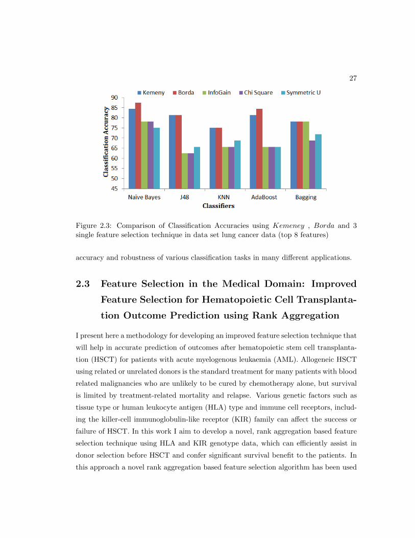
27
Figure 2.3: Comparison of Classification Accuracies using Kemeney , Borda and 3single feature selection technique in data set lung cancer data (top 8 features)
accuracy and robustness of various classification tasks in many different applications.
2.3 Feature Selection in the Medical Domain: Improved
Feature Selection for Hematopoietic Cell Transplanta-
tion Outcome Prediction using Rank Aggregation
I present here a methodology for developing an improved feature selection technique that
will help in accurate prediction of outcomes after hematopoietic stem cell transplanta-
tion (HSCT) for patients with acute myelogenous leukaemia (AML). Allogeneic HSCT
using related or unrelated donors is the standard treatment for many patients with blood
related malignancies who are unlikely to be cured by chemotherapy alone, but survival
is limited by treatment-related mortality and relapse. Various genetic factors such as
tissue type or human leukocyte antigen (HLA) type and immune cell receptors, includ-
ing the killer-cell immunoglobulin-like receptor (KIR) family can affect the success or
failure of HSCT. In this work I aim to develop a novel, rank aggregation based feature
selection technique using HLA and KIR genotype data, which can efficiently assist in
donor selection before HSCT and confer significant survival benefit to the patients. In
this approach a novel rank aggregation based feature selection algorithm has been used

28
Figure 2.4: Comparison of Classification Accuracies using Kemeney , Borda and 3single feature selection technique in data set Internet-ads data (top 60 features)
for selecting suitable donor genotype characteristics. The result obtained is evaluated
with classifiers for prediction accuracy. On an average, this algorithm improves the
prediction accuracy of the results by 3-4% compared to generic analysis without using
feature selection or single feature selection algorithms. Most importantly the selected
features completely agree with those obtained using traditional statistical approaches,
proving the efficiency and robustness of this technique which has great potential in the
medical domain.
2.3.1 Introduction
Approximately 12,000 cases of acute myelogenous leukaemia (AML) are diagnosed an-
nually in the United States. Many patients are not cured by chemotherapy alone, and
require hematopoietic stem cell transplantation (HSCT) for curative therapy. While
HSCT can cure AML, it is a complex procedure with many factors influencing the out-
comes, which remain suboptimal [39]. Donor selection is a critical part of the entire
transplant procedure and researchers are looking for host or donor genetic factors that
can predict a successful outcome after transplantation. For allogeneic HSCT to be suc-
cessful, the leukemia cells must be eradicated by the, combined effect of chemotherapy,
radiotherapy, and a donor T cell mediated graft-versus-leukemia reaction. The donor
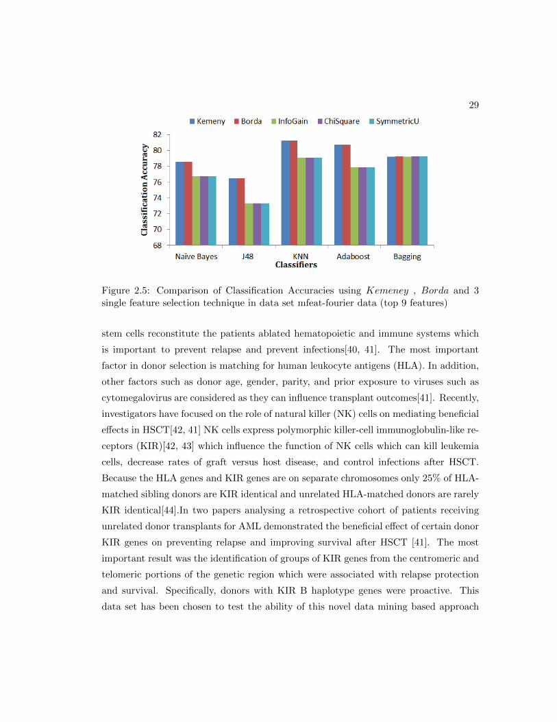
29
Figure 2.5: Comparison of Classification Accuracies using Kemeney , Borda and 3single feature selection technique in data set mfeat-fourier data (top 9 features)
stem cells reconstitute the patients ablated hematopoietic and immune systems which
is important to prevent relapse and prevent infections[40, 41]. The most important
factor in donor selection is matching for human leukocyte antigens (HLA). In addition,
other factors such as donor age, gender, parity, and prior exposure to viruses such as
cytomegalovirus are considered as they can influence transplant outcomes[41]. Recently,
investigators have focused on the role of natural killer (NK) cells on mediating beneficial
effects in HSCT[42, 41] NK cells express polymorphic killer-cell immunoglobulin-like re-
ceptors (KIR)[42, 43] which influence the function of NK cells which can kill leukemia
cells, decrease rates of graft versus host disease, and control infections after HSCT.
Because the HLA genes and KIR genes are on separate chromosomes only 25% of HLA-
matched sibling donors are KIR identical and unrelated HLA-matched donors are rarely
KIR identical[44].In two papers analysing a retrospective cohort of patients receiving
unrelated donor transplants for AML demonstrated the beneficial effect of certain donor
KIR genes on preventing relapse and improving survival after HSCT [41]. The most
important result was the identification of groups of KIR genes from the centromeric and
telomeric portions of the genetic region which were associated with relapse protection
and survival. Specifically, donors with KIR B haplotype genes were proactive. This
data set has been chosen to test the ability of this novel data mining based approach
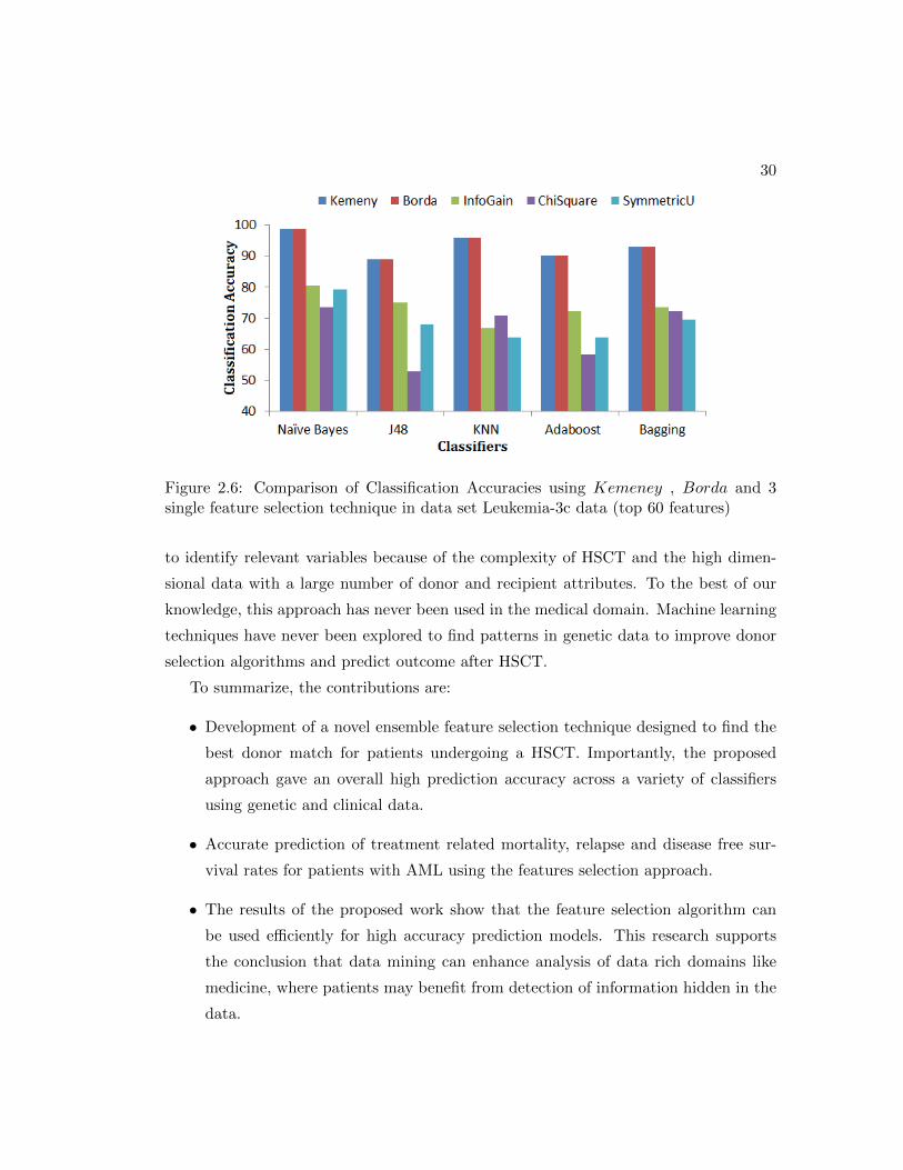
30
Figure 2.6: Comparison of Classification Accuracies using Kemeney , Borda and 3single feature selection technique in data set Leukemia-3c data (top 60 features)
to identify relevant variables because of the complexity of HSCT and the high dimen-
sional data with a large number of donor and recipient attributes. To the best of our
knowledge, this approach has never been used in the medical domain. Machine learning
techniques have never been explored to find patterns in genetic data to improve donor
selection algorithms and predict outcome after HSCT.
To summarize, the contributions are:
• Development of a novel ensemble feature selection technique designed to find the
best donor match for patients undergoing a HSCT. Importantly, the proposed
approach gave an overall high prediction accuracy across a variety of classifiers
using genetic and clinical data.
• Accurate prediction of treatment related mortality, relapse and disease free sur-
vival rates for patients with AML using the features selection approach.
• The results of the proposed work show that the feature selection algorithm can
be used efficiently for high accuracy prediction models. This research supports
the conclusion that data mining can enhance analysis of data rich domains like
medicine, where patients may benefit from detection of information hidden in the
data.

31
Figure 2.7: Comparison of Classification Accuracies using Kemeney , Borda and 3single feature selection technique in data set Arrythmia data (top 36 features)
The remainder of the paper is organized as follows. Section II is the Motivation and
Related works. Section III is the Proposed approach section. Section IV describes the
experimental results. Section V describes the Conclusion.
2.3.2 Motivation and Related Work
Feature selection techniques have immense potential to enhance data mining in the med-
ical domain as has been previously studied in areas such as medical image processing[45,
46, 47, 48]. Ensemble feature selection techniques have been used in the past to improve
robustness and accuracy, but little is known to have been done in the medical domain.
Ensemble methods are advantageous because these can outperform the single feature
selection models when weak or unstable models are combined, mainly because in many
cases several different but equally optimal hypotheses may exist and the ensemble re-
duces the risk of choosing a wrong hypothesis. Another advantage of ensemble methods
is that in contrast to learning algorithms, which may end up in different local optima,
ensemble may give a better approximation of the true function[49, 50].
This data set has been chosen in part because it is high dimensional with missing
data, characteristic of real biologic data, and because it has been extensively studied by
traditional bio-statistical methods to provide good gold standard results to compare the

32
Figure 2.8: Comparison of Classification Accuracies using Kemeney , Borda and 3single feature selection technique in data set AML data (top 25 features)
findings. This data set is unique in that the donor and recipients of URD HSCT were
genotyped not only for their HLA alleles, but also for the NK receptor KIR genes. It
is known that the interactions between KIR and HLA molecules (their natural ligands)
affect the function of NK cells and their ablity to kill cancer cells and to function
to fight infection and promote overall immunity[42, 43, 51, 52, 53]. Several studies
have documented the interaction between HLA and KIR on outcomes after HSCT [54,
55, 56, 57]. The data set used here was described in the first study to demonstrate
that both centromeric and telomeric KIR genes from group B haplotypes contribute
to relapse protection and improved survival after URD HSCT for AML [41, 40].The
authors performed multivariate statistical analyses to identify genetic factors related to
KIR that improve outcome after HSCT. The models included many donor and recipient
transplant and demographic variables known to affect the outcome of HSCT.
The previously published analyses of this data set were designed to develop a decision
strategy to efficiently select the optimal donor to prevent relapse after transplant and
to improve survival. The methodologies used in these studies were generally classical
statistical tests of hypotheses generated by physicians trying to interpret a plethora of
variables based on prior knowledge. However, this approach, while highly accurate, is
time consuming and potentially limited by the biases of the researchers generating the

33
Figure 2.9: Comparison of Classification Accuracies using Kemeney , Borda and 3single feature selection technique in data set Madelon data (top 40 feature)
hypotheses. In any medical condition, treatment decisions can be challenging. The
ultimate decision especially in case of transplants, rest with the physicians, who may be
overwhelmed with a confusing range of information sources. The data is huge in medical
domain and human beings have a limited ability to retain information as compared to
the artificial intelligence, and this worsens when the amount of information increases. As
a result, often there may be undue influence from personal experience. In such situations
data mining can be a blessing where the automated techniques of significant variable
selection can provide to medical experts, the advantage of having a supporting second
opinion for a more accurate decision making. Using data mining, interesting rules and
relationships can be sought and discovered without the need for prior knowledge. Data
mining in general helps to capture cumulative experience of all the patients reflected
in the entire database which can exhibit unknown pattern of medical significance. In
this regard, feature selection can prove to be a highly efficient approach for detecting
the contributing variables from an entire database. The result obtained from feature
selection is a set of highly significant variables which can be used for accurate prediction
purpose, either using classification techniques or statistical approaches. In this paper
I aim at providing the medical domain with a novel feature selection approach which
will help the domain experts in donor selection for a successful HSCT outcome. In
medical domains like HSCT, no research is known to have been conducted to the best
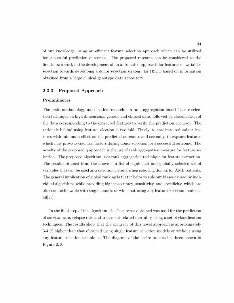
34
of our knowledge, using an efficient feature selection approach which can be utilized
for successful prediction outcomes. The proposed research can be considered as the
first known work in the development of an automated approach for features or variables
selection towards developing a donor selection strategy for HSCT based on information
obtained from a large clinical genotype data repository.
2.3.3 Proposed Approach
Preliminaries
The main methodology used in this research is a rank aggregation based feature selec-
tion technique on high dimensional genetic and clinical data, followed by classification of
the data corresponding to the extracted features to verify the prediction accuracy. The
rationale behind using feature selection is two fold. Firstly, to eradicate redundant fea-
tures with minimum effect on the predicted outcomes and secondly, to capture features
which may prove as essential factors during donor selection for a successful outcome. The
novelty of the proposed q approach is the use of rank aggregation measure for feature se-
lection. The proposed algorithm uses rank aggregation technique for feature extraction.
The result obtained from the above is a list of significant and globally selected set of
variables that can be used as a selection criteria when selecting donors for AML patients.
The general implication of global ranking is that it helps to rule out biases caused by indi-
vidual algorithms while providing higher accuracy, sensitivity, and specificity, which are
often not achievable with single models or while not using any feature selection model at
all[58].
In the final step of the algorithm, the feature set obtained was used for the prediction
of survival rate, relapse rate and treatment related mortality using a set of classification
techniques. The results show that the accuracy of this novel approach is approximately
3-4 % higher than that obtained using single feature selection models or without using
any feature selection technique. The diagram of the entire process has been shown in
Figure 2.10
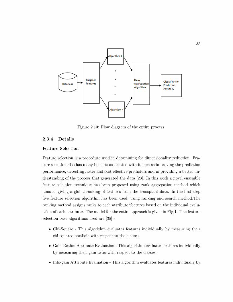
35
Figure 2.10: Flow diagram of the entire process
2.3.4 Details
Feature Selection
Feature selection is a procedure used in datamining for dimensionality reduction. Fea-
ture selection also has many benefits associated with it such as improving the prediction
performance, detecting faster and cost effective predictors and in providing a better un-
derstanding of the process that generated the data [23]. In this work a novel ensemble
feature selection technique has been proposed using rank aggregation method which
aims at giving a global ranking of features from the transplant data. In the first step
five feature selection algorithm has been used, using ranking and search method.The
ranking method assigns ranks to each attribute/features based on the individual evalu-
ation of each attribute. The model for the entire approach is given in Fig 1. The feature
selection base algorithms used are [38] -
• Chi-Square - This algorithm evaluates features individually by measuring their
chi-squared statistic with respect to the classes.
• Gain-Ration Attribute Evaluation - This algorithm evaluates features individually
by measuring their gain ratio with respect to the classes.
• Info-gain Attribute Evaluation - This algorithm evaluates features individually by

36
measuring their Information gain with respect to the classes.
• Symmetrical Uncertainty - This algorithm evaluates features individually by mea-
suring their symmetrical uncertainty with respect to the class.
• Filtered Attribute evaluation - an arbitrary attribute evaluator on data that has
been passed through an arbitrary filter
By applying the above algorithms to all features, five lists of ranked attributes has
been generated on same data. Then the rank aggregation algorithm has been applied
over the five sets of ranks generated for each attribute to produce a global ranking of
the attributes based on their significance level. Feature selection techniques such as
Principle Component Analysis or SVM has not been used in this work because these
algorithms scale the actual features in high dimensional space to produce synthetic
features. Loosing the original features makes it difficult to interpreted the results in the
medical domain where decision making relies on selection of original features.
Rank Aggregation
I propose an algorithm which uses a novel rank aggregation technique for assigning a
global rank on the features which is uninfluenced by ranking algorithm biases. Rank
aggregation can be done in various ways [22, 32]. The rank aggregation approach used in
this algorithm is a modified version of rank aggregation method used for web searches[22,
32]. The mathematical formulation is shown in Equation 2.3-
Rankglobal =1
n
n∑i=1
Rankn (2.3)
where n is the number of list generated from n number of feature selection algo-
rithms. Rankglobal is the global rank obtained after rank aggregation on the ranks ob-
tained from n algorithms.
The benefit of using this approach is that, no prior knowledge about the contribution
of each features or variables are needed since the actual rank produced by each feature
selection algorithm is used as the contributing factor for the proposed rank aggregation
based feature selection algorithm.
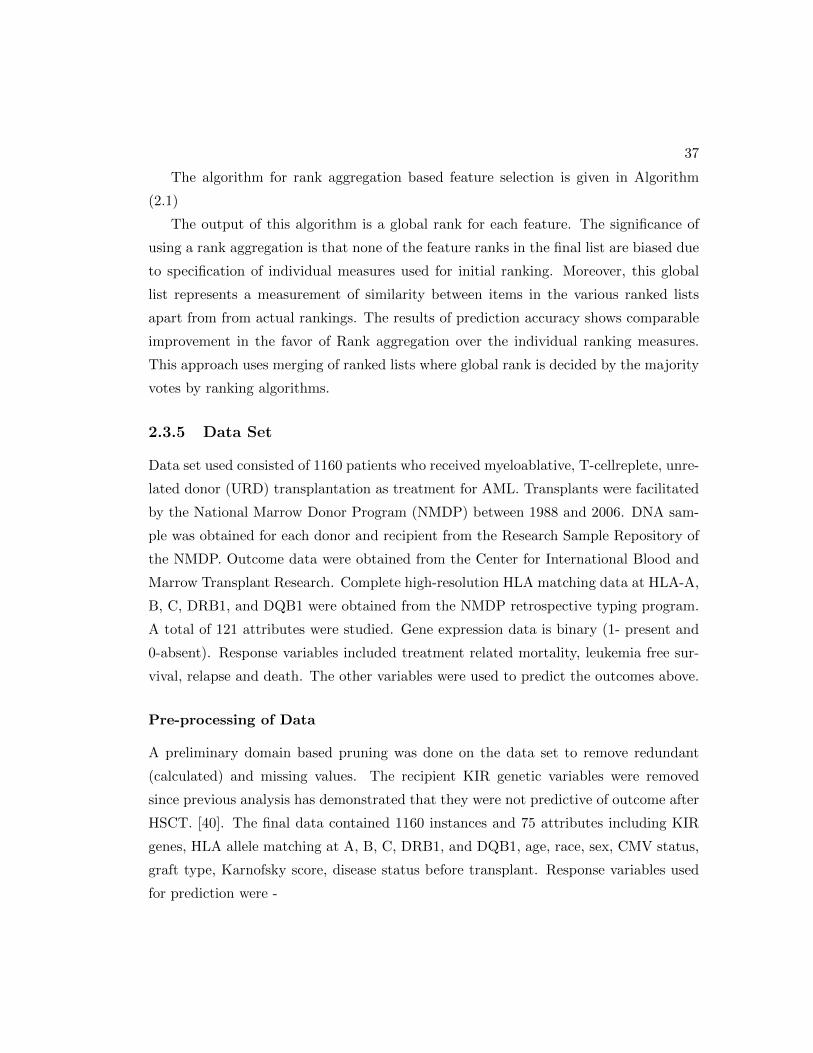
37
The algorithm for rank aggregation based feature selection is given in Algorithm
(2.1)
The output of this algorithm is a global rank for each feature. The significance of
using a rank aggregation is that none of the feature ranks in the final list are biased due
to specification of individual measures used for initial ranking. Moreover, this global
list represents a measurement of similarity between items in the various ranked lists
apart from from actual rankings. The results of prediction accuracy shows comparable
improvement in the favor of Rank aggregation over the individual ranking measures.
This approach uses merging of ranked lists where global rank is decided by the majority
votes by ranking algorithms.
2.3.5 Data Set
Data set used consisted of 1160 patients who received myeloablative, T-cellreplete, unre-
lated donor (URD) transplantation as treatment for AML. Transplants were facilitated
by the National Marrow Donor Program (NMDP) between 1988 and 2006. DNA sam-
ple was obtained for each donor and recipient from the Research Sample Repository of
the NMDP. Outcome data were obtained from the Center for International Blood and
Marrow Transplant Research. Complete high-resolution HLA matching data at HLA-A,
B, C, DRB1, and DQB1 were obtained from the NMDP retrospective typing program.
A total of 121 attributes were studied. Gene expression data is binary (1- present and
0-absent). Response variables included treatment related mortality, leukemia free sur-
vival, relapse and death. The other variables were used to predict the outcomes above.
Pre-processing of Data
A preliminary domain based pruning was done on the data set to remove redundant
(calculated) and missing values. The recipient KIR genetic variables were removed
since previous analysis has demonstrated that they were not predictive of outcome after
HSCT. [40]. The final data contained 1160 instances and 75 attributes including KIR
genes, HLA allele matching at A, B, C, DRB1, and DQB1, age, race, sex, CMV status,
graft type, Karnofsky score, disease status before transplant. Response variables used
for prediction were -

38
• Treatment Related Mortality - Indicator of death of patients which is only caused
due to post treatment effects such as acute or chronic graft verses host disease
which develops in a patient within a given period of time.
• Relapse Free Survival - Indicating whether the patient survived after BMT treat-
ment without having a relapse, after a certain amount of time decided by the
medical experts.
• Relapse Rate - indicating whether the patient had a relapse of AML
Evaluation
In order to evaluate the performance of the proposed algorithm, the classification accu-
racy has been compared between the prediction on the feature subset produced using
the proposed rank aggregation technique with prediction on the unprocessed features
without using feature selection technique prior to model building for classification. The
comparison of accuracy between the rank aggregation algorithm selected features and
the results from the individual feature selection algorithm selected features have been
considered in this paper as an additional evaluation criteria for the rank aggregated
features. The mathematical formulation of accuracy measure A is given in 2.4
Accuracy =C
C ′(2.4)
where C is the Number of correctly classified samples and C ′ is the Total number of sam-
ples
Classification Algorithms
The different classification algorithms used are - Decision Tree / AdTree, AdaBoost with
Decision Stump or JRip, SMO, Logistic Regression, Voted Perceptron and Bayesian
Network. The main reason behind using a wide range of classification algorithms is
to demonstrate the robustness of the proposed approach. The proposed algorithm can
be used along with a variety of Prediction measures including rule based, Bayesian
Network. classification tree, ensemble based and even statistical measure like regression.

39
It has been shown in the result section that using this algorithm, a consistent prediction
accuracy can be achieved across all the classifiers.
2.3.6 Experimental Results
In order to confirm the reliability of the proposed approach and to accurately predict
characteristics of a donor which are associated with improved outcome after HSCT
for AML, a comparative analysis was conducted using the prediction results of the
proposed algorithm with that of the traditional statistical approaches [40, 41] given in
Table 2.20. The Table 2.20 demonstrates the statistically significant variables that are
selected by multivariate analysis with 95% Confidence Interval for relapse free survival
after transplant. These are - Disease Status , donor race, HLA matched/mismatched,
Karnofsky, Performance Status, Age(categorical), Specific KIR Genes, Centromeric and
Telomeric KIR groups, transplant (per year) and KIR B Content status. The features
selected by the proposed approach, in the first column of the Table 2.20 shows that,
the proposed algorithm has been able to correctly capture the significant variables. All
the statistically significant variables have been detected as the top ranked features with
in top 15 by our rank aggregation algorithm. Moreover the proposed algorithm also
detected other important variables including - conditioning regimen during transplant,
characterization of the AML as primary or secondary, donor and recipient sex match and
graft source during transplant (bone marrow vs. peripheral blood derived stem cells).
The results show that the proposed rank aggregation-based feature selection data mining
algorithm could detect not only the previously identified statistically significant features,
but also other novel features which had not been detected by any other approach. These
results will direct physicians to explore other dimensions of donor characteristics which
may have been overlooked. This is one of the several advantages of data mining; to
detect hidden patterns which are not otherwise visible through human judgement or
prior knowledge based variable detection.
Next, the output of the proposed rank aggregation algorithm was analyzed and eval-
uated. classification was performed using the selected top 35 features to predict the sur-
vival rate, treatment related mortality rate, and relapse rate for patients with AML. A
heuristic approach was used to determine the number of top features to select from the 75
ranked features.

40
Figure 2.11: Classification Accuracy for treatment related mortality
Apart from the accuracy comparison , a comparative analysis of the result of classi-
fication on unprocessed features vs results obtained on using our rank aggregation algo-
rithm has been performed. There is a striking 3-4% approximate overall improvement
in the prediction. In figure 2.12 the prediction accuracy of survival rate is depicted. Our
algorithm gives an additional 3-4% accuracy while predicting treatment related mortal-
ity. Similar trend can be seen in prediction accuracy comparisons for treatment related
mortality and Relapse rate shown in Figure 2.12 and 2.13. These results shows that the
proposed algorithm gives a constant high accuracy for different kinds of classification
algorithms as compared to when the features are used without applying the proposed
algorithm. Another, important factor of the proposed rank aggregation algorithm is
that, this approach is more robust as compared to when classifying with all the fea-
tures. This algorithm is also scalable since the time complexity is in the order of O(n)
for the rank aggregation part of our algorithm. The classification algorithms has been
used with Weka [38] which can handle huge amounts of datasets.
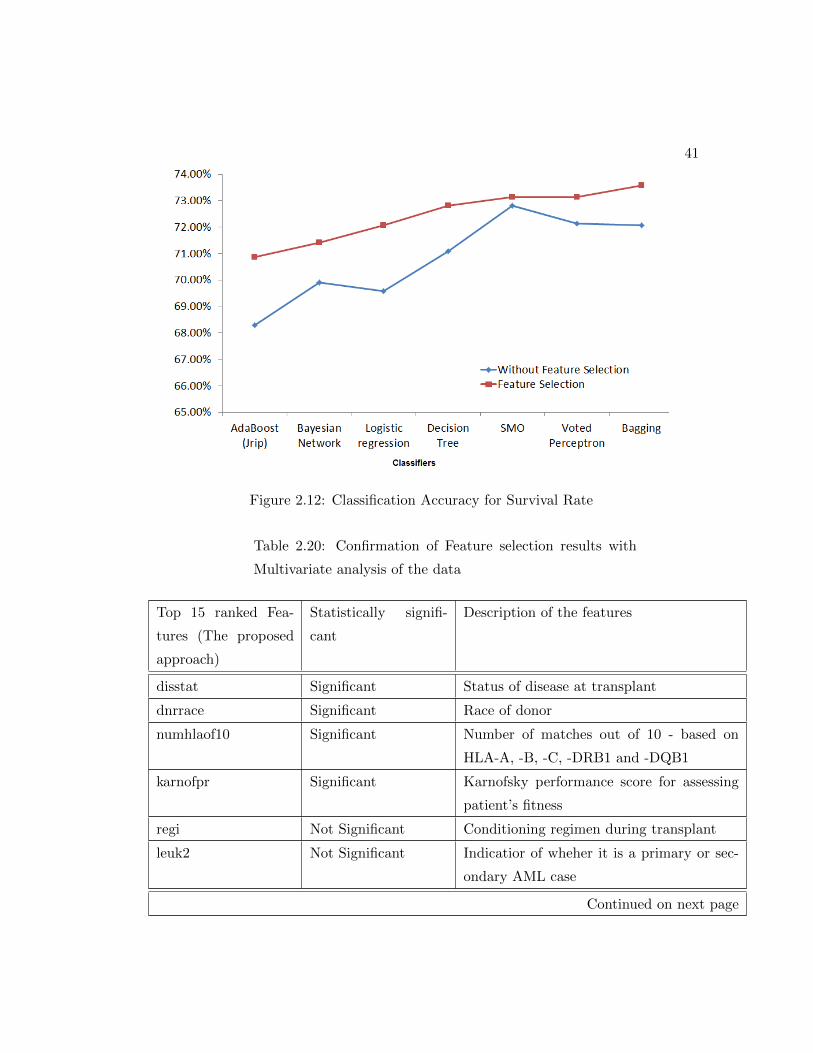
41
Figure 2.12: Classification Accuracy for Survival Rate
Table 2.20: Confirmation of Feature selection results with
Multivariate analysis of the data
Top 15 ranked Fea-
tures (The proposed
approach)
Statistically signifi-
cant
Description of the features
disstat Significant Status of disease at transplant
dnrrace Significant Race of donor
numhlaof10 Significant Number of matches out of 10 - based on
HLA-A, -B, -C, -DRB1 and -DQB1
karnofpr Significant Karnofsky performance score for assessing
patient’s fitness
regi Not Significant Conditioning regimen during transplant
leuk2 Not Significant Indicatior of wheher it is a primary or sec-
ondary AML case
Continued on next page

42
Table 2.20 – continued from previous page
dagecat Significant Age category of donor
Donor Neutral
Better Best
Significant Number of centromeric and telomeric gene
content motifs containing B haplotype KIR
genes
numtx Significant Total number of transplants the recipient
has had
sexmatch Not Significant Donor and recipient sex match
graftype Not Significant Graft source : Bone marrow, PBSC, Cord
blood
Donor Final Centro
Grp
Significant Centromeric KIR group - Cen A/A, Cen
A/B, Cen B/B
Donor 2DS4 Length
Groups
Significant Presence or absence of Specific KIR Genes
Donor Final Telo Grp Significant Presence or absence of Telomeric group -
Telo A/A, Telo A/B, Telo B/B
In figures 2.11, 2.12 and 2.13 It can be seen that accuracy of the proposed approach is
almost consistent with different classification models. In contrast, the accuracy measure
of classification based on the unprocessed features are fluctuating and model dependent.
The main reason behind this, is the fact that this algorithm assigns a global rank which
is not influenced and biased by individual feature selection models. Hence, robustness
is preserved across all the classification models used. In Figure 2.14, the prediction
accuracy has been analyzed from the rank aggregation based feature selection with that
of individual feature selection models such as Chi Square based, Gain ratio , infogain
, filter based and Symmetrical Uncertainty based feature selection models. This result
shows that the proposed approach gives a constant higher accuracy than that of other
single feature selection models over a variety of classification algorithms for predicting
survival rate. Overall, the proposed approach gives a better result proving it has great
potential in medical domain with significant benefits.
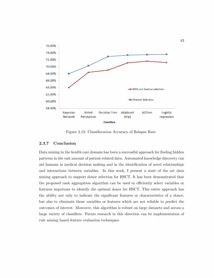
43
Figure 2.13: Classifiecation Accuracy of Relapse Rate
2.3.7 Conclusion
Data mining in the health care domain has been a successful approach for finding hidden
patterns in the vast amount of patient-related data. Automated knowledge discovery can
aid humans in medical decision making and in the identification of novel relationships
and interactions between variables. In this work, I present a state of the art data
mining approach to support donor selection for HSCT. It has been demonstrated that
the proposed rank aggregation algorithm can be used to efficiently select variables or
features important to identify the optimal donor for HSCT. This entire approach has
the ability not only to indicate the significant features or characteristics of a donor,
but also to eliminate those variables or features which are not reliable to predict the
outcomes of interest. Moreover, this algorithm is robust on large datasets and across a
large variety of classifiers. Future research in this direction can be implementation of
rule mining based feature evaluation techniques.

44
Figure 2.14: Classification Accuracy of Survival Rate for comparing rank aggregationalgorithm vs single feature selection algorithms

Chapter 3
Predictive Overlapping
Co-clustering for Heterogeneous
data
In the past few decades co-clustering has emerged as an important data mining tool
for exploratory analysis and decision making. However, one of the overlooked benefits
of co-clustering is its ability to improve predictive modeling. Several applications such
as finding gene expression profiles, patient-disease cohorts in health care analysis, user-
item groups in recommendation systems and community detection problems can benefit
from technique that utilizes the predictive power of the data to generate co-clusters.
In this work, the novel idea of Learning based Co-Clustering (LCC) has been pre-
sented as an optimization problem for an effective and improved predictive analysis.
The algorithm proposed in this research generates co-clusters by maximizing its pre-
dictive power subject to constraints on the number of co-clusters. It has been shown
with extensive empirical evaluation in diverse domains that this method generates co-
clusters that improves predictive power of learning model, as high as 10% over the
original data set. This paper also demonstrates that LCC has better performance than
two state-of-the-art co-clustering methods namely, Spectral Co-clustering and Bayesian
Co-clustering. The algorithm has been evaluated using two benchmark and two real
world data sets. The results demonstrate the effectiveness and utility of the proposed
45

46
algorithm in practice.
3.1 Introduction
Hidden homogeneous blocks of data commonly referred as co-clusters [16] has been
found to provide significant advantages to several application domains. For example,
one may be interested in finding groups of patients that show similar activity pattern
under a specific subset of health care conditions [59], simultaneously clustering movies
and user ratings in collaborative filtering [60], finding document and word clusters in
text clustering [61] or grouping genes with similar properties based on their expression
patterns under various conditions or across different tissue samples in bio-informatics
[62, 63]. One of the overlooked advantages of co-clustering is that it can be used as
a data segmentation process for improving predictive modeling. This is because, in
real world problems, the presence of insignificant features and extraneous data can
greatly limit the accuracy of learning models built on the data. Therefore, instead of
building predictive models on data from a noisy domain, homogeneous groups can be
extracted by segmenting the data for building more effective predictive models. The
various types of data segmentation process has been shown in figure 3.4 which shows
that co-clustering falls in the category of data segmentation across both row as well as
column dimensions. Co-clustering find application in several domain including targeted
marketing and recommendation. Motivated by this, in this work presents a novel co-
clustering algorithm called Learning based co-clustering (LCC). The key idea of the
proposed algorithm is to generate optimal co-clusters by maximizing predictive power
of the co-clusters subject to the constraints on the number of co-clusters. The resulting
clusters are high in predictive power (for example classification accuracy, f-measure)
when a learning (classification) model is built on them.
The proposed algorithm has the added advantage that, co-clusters generated are
overlapping in nature. Most importantly, there is no need to pre-specify the number
of co-cluster as a parameter. Most of the existing co-clustering algorithm focuses on
finding co-clusters with single membership of a data point in the data matrix [61]. Al-
though these techniques generate efficient results over real data set, these algorithms are
based on the assumption that, a single data point can belong to only one cluster. This
47
assumption is often not completely valid since, in real life there is a high probability that
a single data point belongs to multiple clusters with varying degree of its membership
with the clusters. For example, in recommendation system a group of user may prefer
pop music as well as country music. In fact, several real life situations that deal with
high dimensional data with heterogeneous population can benefit more from finding
co-clusters that overlap each other. One important example can be finding co-cluster
from Electronic Health Records or EHR (hospital data) for predictive analysis in health
care. EHR data in health care is often high dimensional with heterogeneous population
that makes co-clustering a suitable approach for finding groups of patients and disease
conditions. However, each of these co-clusters of patient-disease condition should reflect
patient sub-populations that potentially share co-morbid diagnoses. Hence, in this sce-
nario detecting overlapping co-clusters would help capture the most utilizable pattern
that exists in the data.
In co-cluster analysis, detecting good co-clusters is a non-trivial task. This is because
in most of the real life data analysis problems, data is very high dimensional and consists
of noise in the form of extraneous instances and insignificant features. Co-clusters
extracted from these data might not be suitable for a specific supervised learning purpose
if these co-clusters have been obtained from a complete unsupervised setting. In real life
applications often predictive models are built on segmented data using domain expert’s
knowledge [64]. In such situation assigning a specific supervised learning algorithm
to a co-cluster becomes a challenge. In this work, a co-clustering algorithm has been
developed as well as a testing framework has been proposed that takes into account the
class information to remove noise from the data resulting in co clusters that improves
the predictive power of learning models built on them.
The LCC has been defined as an optimal co-clustering that minimizes the “loss”
in predictive power (or maximizes the “gain” in predictive power). The goal of this
algorithm is to seek a “soft” clustering [65] of both dimensions such that the “gain”
in ”Predictive Power” of the co-clusters is maximized given an initial number of row
and column clusters. The number of co-cluster to be generated doesn’t need to be
pre-specified and is upper-bounded by maximum number of co-clusters to be generated
through an initial number of row and column clusters. It has been assumed that, class
information is available for evaluating the predictive power of a learning model built
48
using co-clusters.
The row clusters are generated by identification of a distinguished soft partition of
the data matrix in the row dimension such that data point belonging to a partition
has strong intra-object resemblance. The column clusters are generated in a similar
way. The optimal clustering criteria for a soft partition has been obtained using gen-
eralized least squared error functions [65]. The proposed algorithm is suitable for high
dimensional data because it reduces dimensions iteratively by removing noisy rows and
columns. The result of the proposed algorithm is a set of overlapping co-clusters with
reduced row and column noise and a higher predictive power than the original data.
Four data sets have been used from diverse domain such as health care and movie
recommendation. For evaluation co-clusters generated using LCC has been compared
with the original data set. The performance of LCC has also been compared with
two traditional co-clustering algorithms. Evaluation measures used are classification
accuracy, f-measure, cluster-precision, cluster-recall and cluster-f-measure calculated
over pairs of points. The main contributions of this work are -
1) The concept of a co-clustering has been proposed that is dedicated towards im-
proving predictive modeling.
2) A novel co-clustering algorithm has been proposed which generates overlapping
co-clusters that improves predictive modeling. An important property of this
algorithm is that there is no need to specify the number of co-clusters.
3) A separate model testing framework has been proposed, with test data for reducing
model over fitting and for a more accurate result.
4) In this research, it has been demonstrated that the proposed algorithm work
well on benchmark as well as real world data sets. Empirical results show that,
the proposed approach yields co-clusters that improves the predictive power of a
learning model significantly.
3.2 Related Work
Co-clustering has become a topic of interest in the past few decades due to its success
and usability in numerous important applications such as for finding gene expression

49
patterns [66], document and word clustering [67], clustering tags and social data sources
[68], recommendation systems [60]. Co-clustering has been applied successfully in other
areas such as Biological networks [69], medical imaging [70], co-clustering of denatured
hemoglobin [71]. Popular techniques of co-clustering are bipartite spectral graph parti-
tioning [67], information-theoretic co-clustering [61], and Bayesian co-clustering [72].
The earliest works in co-clustering was done in 1972 using hierarchical row and
column clustering in matrices by a local greedy splitting procedure [73]. In this paper,
the author proposed a hierarchical partition based two way clustering algorithm that
splits the original data matrix into set of sub-matrices and used variance for evaluating
the quality of each sub matrix. Later this method was improved by [74] that introduced
a backward pruning method for generating an optimal number of two way clusters.
In Information theory domain [75] proposed an approach called “Information bot-
tleneck theory” that was developed for one dimensional clustering. Later [61] extended
their work and proposed a co-clustering technique using the concepts of information the-
ory. Another important paper [67] proposed a co-clustering technique that was modeled
based on bi-partite graphs and their minimal cuts.
Most of the works in the past have focused on “crisp” or partition based co-clustering
and very few recent research can handle overlapping co-clusters [72]. Even for one-way
clustering, there are few algorithms known as “soft” clustering algorithms which can
identify overlapping clusters. One of the earliest example is fuzzy c-means clustering
[65]. One of the notable works in overlapping co-clustering was [16] where the authors
have proposed an overlapping co-clustering model that can be applied with a variety of
clustering distance functions. Other important works in overlapping co-clustering that
has been shown to be of immense utility in various fields includes [76], [77] and [78].
There are very few works in the past, to the best of our knowledge that utilizes pre-
dictive power of a data matrix to generate co-clusters. A recent work on semi supervised
co-clustering is by [79]. In this paper the authors finds optimal co-clustering by incor-
porating in the clustering process, prior information regarding the existence of certain
objects and features. For this they use a matrix decomposition approach and solve co
clustering problem as a trace minimization problem. Another relevant work is by [80]
where a semi-supervised co-clustering technique has been developed that captures the
inherent structure of complex data and predicts missing entries by constructing simple
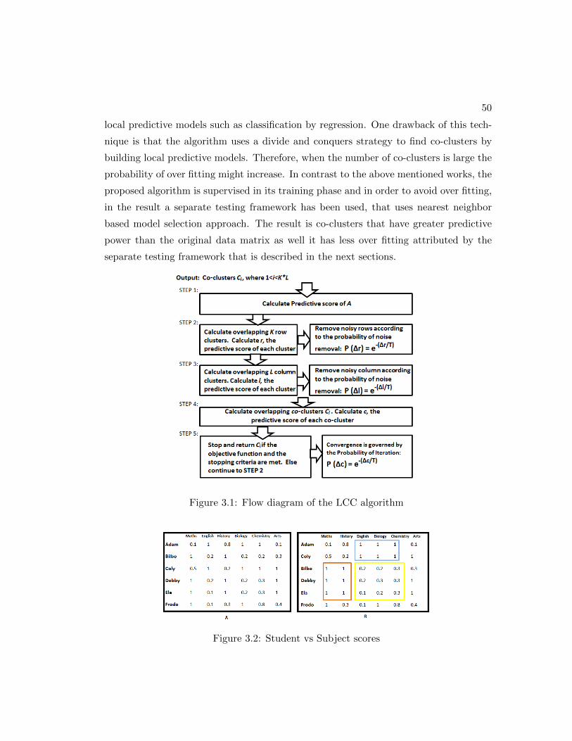
50
local predictive models such as classification by regression. One drawback of this tech-
nique is that the algorithm uses a divide and conquers strategy to find co-clusters by
building local predictive models. Therefore, when the number of co-clusters is large the
probability of over fitting might increase. In contrast to the above mentioned works, the
proposed algorithm is supervised in its training phase and in order to avoid over fitting,
in the result a separate testing framework has been used, that uses nearest neighbor
based model selection approach. The result is co-clusters that have greater predictive
power than the original data matrix as well it has less over fitting attributed by the
separate testing framework that is described in the next sections.
Figure 3.1: Flow diagram of the LCC algorithm
Figure 3.2: Student vs Subject scores

51
3.3 Problem Definition
Let C represents the data matrix denoting a m × n matrix. Each object in C belongs
to instances from the rows X represented as x1, x2, ..., xm and features from columns Y
represented as y1, y2, ..., yn.
The primary interest lies in generating co-clusters (X, Y ) from C by clustering X
and Y into k and l ”soft” clusters respectively, and removing noisy instances and fea-
tures from the data. Let k clusters of X be denoted as x1, x2, ..., xk and l clusters of Y be
denoted as y1, y2, ..., yl. Let the clustering function for row and columns be formulated
as MX and MY defined as
X = MX(X) = x1, x2, ..., xm −→ x1, x2, ..., xk
Y = MY (Y ) = y1, y2, ..., yn −→ y1, y2, ..., yl.
Definition 1 Refer (MX ,MY ) as a co-clustering.
The challenge is to find a co-clustering (MX ,MY ) that improves the learning task
of a learner built on the co-clusters. This denotes, a learning model should be able
to predict the labels for all unlabeled rows in X and Y with an improved accuracy or
f-measure when compared with prediction result of the learner built with X using C.
An assumption made here is the availability of class labels for all X in the training
phase.
3.4 An Intuition of the Proposed Approach
Let us consider a toy example given in Figure 3.2 A. It contains six instances and six
features represented by students and their subject scores (in a scale of 0 to 1). Let us
assume a set of class labels as ‘decision of admission in school’. The problem is to predict
an admission decision for a new student. For a diverse population of students and a
wide range of subjects, in which a student’s performance is scored, it is unlikely that all
student - subject scores can be explained using a single learning model. An alternative
and a more meaningful solution would be to learn models that closely represent the
scores for only a subset of students over a subset of subjects. In this scenario, one
52
could suggest an independent one-dimensional clustering on both the row and column
dimensions and built learning models later on all possible combination of instances and
features. However, in this case, the choice of co-clusters for building models can increase
well beyond it is actually required. Most importantly, choosing the best co-cluster for a
given model is a non-trivial task. Lastly, co-cluster purity estimation will be challenging
in such a process. The proposed algorithm on the other hand generates co-cluster based
on predictive capability of the data matrix for a given learning model.
The motivation of noise removal is that, in a co-clustering process, if all instances
and features are included in the resulting co-clusters, the results of the learning models
built on the co-clusters might be poor since some instances and features might contribute
negatively for learning a model (the quality of the result has been examined as Predictive
power in the algorithm section below. For the moment it can be assumed that the
results are poor). In this algorithm, the data matrix has been co-clustered such that,
instances and features can be identified which do not contribute to learning models
on the co-clusters. This information can be eliminated(the extraneous and wrongly
recorded instances and insignificant features can be referred as noise) for improving the
cluster assignment in an iterative way. For example Figure 3.2 B, represents the final
co-clustering result of the student-subject score matrix. Note that while blocks of scores
representing student-subject pairs are detected, not all instances or features has been
included to be a part of the co-clusters since these might contributes negatively in the
model learning process with the co-clusters. The detection and elimination of noise in
the algorithm is not ad hoc or arbitrary. For example, noise is detected with the help of
a predictive model on the co-clusters in every iteration so that LCC algorithm does not
reach a local optima. For this, an optimization process has been used namely, simulated
annealing [81], described in the later sections.
3.5 Learning Based Co-clustering Algorithm
In this paper, a Learning based co-clustering (LCC) algorithm has been developed, that
identifies overlapping co-clusters from high dimensional data. LCC can be considered
as a variant of two way co-clustering algorithms [82]. In two-way co-clustering, separate

53
Figure 3.3: Intuitive proof of row column rearrangement result for co-cluster generationas given in algorithm 3.1
one dimensional clustering is performed and the result is combined to generate co-
clusters. In this paper, the proposed algorithm generates one dimensional overlapping
clusters [65] from both row and column dimension and improves the co-clusters with an
objective function in successive iterations to find optimal overlapping co-clusters. The
one dimensional clusters are identified using two different scoring mechanisms namely
intra-cluster and inter-cluster distance. Instead of crisp allocation of data points to any
particular cluster, a membership matrix is generated which indicates the membership
of a data point in a single or more than one cluster [65]. A pre-defined membership
threshold has been assumed for the data points in both the dimensions. This threshold

54
Figure 3.4: Various type of Data Segmentation process
allows allocation of data points to one or more than one cluster. After calculating
overlapping clusters from both the dimensions, the co-clusters can be optimized by
removing noisy rows and columns. This is continued in an iterative process until the
stopping criteria is met.
The motivation behind this approach is that, removing redundant or wrongly doc-
umented instances and irrelevant features from the data in form of noise, will assist
in improving the predictive power of a learning model built on the data. The statisti-
cal insights taken from these co-clusters would help effective predictive model building
and an improved decision making. For example, in recommendation systems, finding
user-item co-clusters from a heterogeneous population would help provide guidance for
predicting different genres of a movie for customers with similar interest.
LCC algorithm is interesting as it uses predictive power of the co-clusters to detect
and eliminate noisy rows and noisy columns while co-cluster formation. An added
advantage of LCC is that there is no need to specify the number of co-cluster. Most
importantly, this algorithm seeks to find overlapping or ”soft” co-clusters that might
qualify it as an algorithm that is closely capable of capturing the structure of real world
data.

55
I propose to develop LCC as an iterative algorithm, with co-clusters getting refined
at iterations aided by the threshold of noise removal while maximizing the objective
function. The objective function of LCC defined in equation 4 states that the algorithm
aims to maximize the predictive power of identified co-clusters, subject to the constraints
on the number of co-clusters c and 1 < c < k ∗ l, where k and l are the initial number
of row and column clusters. In equation 4, I call F (X; Y ) as the mean predictive power
of a model learned on the co-clusters generated in any given iterative stage. In general
other aggregate scores such as co-cluster with the the max or min predictive power can
be used. F (X;Y ) is the function that represents the predictive power of a learning
model on original data matrix (X;Y ). The gain in predictive power F (X; Y )−F (X;Y )
can be explained as the quantity that facilitates the search for an optimal co-clustering.
Definition 2 Learning based co-clustering can be defined as
Maximize(F (X; Y )− F (X;Y )) (3.1)
Subject to the constraints on the number of co-clusters c and 1 ≤ c ≤ k ∗ l, where k is
the initial no. of row cluster and l is the initial number of column cluster.
The co-clustering algorithm works as follows. In step 1, a ”soft” row clustering
M(1)X ( M
(t)X with tth iteration ) is obtained from C. The predictive power of each row
cluster x1, x2, ..., xk (let it be ρrow1, ρrow2, ..., ρrowk ) is compared with the predictive
power of (X;Y ), (let’s call it ρ) assuming the availability of the class label information.
The noise removal task is controlled in each iteration with a threshold τrow and τcol,
namely, noise removal threshold and Prow and Pcol, namely, probability of row noise and
colum noise removal respectively. Prow and Pcol is calculated using a probabilistic meta-
heuristic known as simulated annealing [81] described in equation 3.2. ∆ρ represents
the absolute gain in predictive power of a row cluster as compared to that of the dataset.
T is the cooling schedule parameter that controls the probability P and hence, avoids
this process from reaching a bad local optima. If Prow for a given iteration meets the
constraint τrow, it denotes the probability of removing noisy row is optimum in the
current iterative stage. If any of ρrow1, ρrow2, ..., ρrowk meets the threshold τrow, those
rows exclusively belonging to the row cluster (and not other row clusters, since this is
56
an overlapping clustering) is discarded as noise. C is updated to C ′ with remaining
rows.
P = e−∆ρ/T (3.2)
In step 2, a ”soft” column clustering M(1)Y is obtained from C. The predictive power
of each column cluster y1, y2, ..., yl (let it be ρcol1, ρcol2, ..., ρcoll) is compared with ρ,
assuming presence of same class label information. A probability threshold τcol has
been assigned for comparison and determining if a column cluster should be considered
as a noisy column cluster. Using simulated annealing [81] the algorithm determines Pcol,
the probability of a column cluster to be considered as a noise. If Pcol as calculated from
equation 3.2 meets the constraint τcol for a given iteration, it denotes the probability
of removing noisy column is optimum in the current iterative stage. ∆ρ in equation
3.2 represents the absolute gain in predictive power of a column cluster as compared to
that of the dataset. If any of ρcol1, ρcol2, ..., ρcoll does not meet τcol, it is not removed.
C ′ is updated to C ′′ with rest of the columns.
In step 3, co-clusters are generated from the C using algorithm 3.1 with remaining
rows and column indexes from M(1)X and M
(1)Y . Co-clusters has been generated as
follows - remove row noise while row wise soft clustering followed by column noise
removal while column wise soft clustering. Re-order the X such that all rows in X
belonging to x1 cluster are arranged first. Followed by all rows in X belonging to x2
and so on. Similarly, Re-order the Y such that all rows in Y belonging to y1 cluster are
arranged first. Followed by all rows in Y belonging to y2 cluster are arranged and so on.
The result is that the data matrix is divided into small two dimensional blocks which
denoted as co-clusters as given in algorithm 3.1. It should be noted that the effect of
rearranging the rows and column according to their respective row and column clusters
stays the same even if the cluster rearranging order is changed. This has been explained
using the toy example using figure 3.3 that was introduced in figure 3.2 . From figure
3.3 it is clear that , one will arrive at the same co-clusters/ blocks of data if the row
first arrangement is performed followed by column rearrangement or vise-versa. Next,
the algorithm checks if the newly formed co-clusters meets the stopping criteria given in
section 3.3. If it is not met, the algorithm proceeds to step 1 with C′′. This check is done
iteratively. The algorithm generates co-clustering (M(2)X ,M
(2)Y ), (M
(3)X ,M
(3)Y )... , stores

57
the co-clustering result with the best predictive score and iterates until the stopping
criteria is met. It outputs co-clusters according to the stopping criteria described in the
next section.
The notations has been shown in table 3.14 for the ease of understanding and refer-
ence. As the cluster mapping function MX , MY has been used fuzzy C-means clustering
[83], which is a soft one dimensional clustering algorithm. Fuzzy C-means [83] is based
on the concept of a membership vector ~V = ~v1, ~v2, .. ~vp that indicates the membership
probability of an object with p clusters. The membership probability of each vector
component varies between 0 to 1. The membership denotes the probabilistic distance
of an object with the cluster. Hence,∑p
i=1 ~vi = 1. i.e. sum of all the membership
probabilities for a given object is one. In order to assign objects to the base cluster, a
fixed threshold membership probability has been assumed. This helps in allocation of
objects in different clusters (same object can get allocated to multiple clusters) for the
algorithm.
Table 3.1: Generate Co-clusters Algorithm
Algorithm
Input:Data Matrix C′′, row clusters x1, x2, ..., xk, column clusters y1, y2, ..., yk
Output: co-clusters c
Steps:
1. Re-order the X such that all rows in X belonging to x1 are arranged first. Followed
by all rows in X belonging to x2 and so on.
2. Re-order the columns in Y such that all columns in Y belonging to y1 are arranged
first, followed by all columns in Y belonging to y2 and so on.
3. Output c small two dimensional blocks generated from dividing C′′
by reordering
the rows and columns by row clusters and column clusters. An intuitive proof that that
reordering in any direction yields the same c co-clusters has been given in figure 3.3

58
3.5.1 Stopping Criteria
The stopping criteria of the proposed algorithm assist in finding an approximately op-
timal solution. This task is non-trivial since there is always a chance that the algo-
rithm will end with a local optimal solution. Therefore, a probabilistic neighborhood
search approach namely, Simulated annealing [81] with a control parameter called cool-
ing schedule has been used. This control parameter has been referred as T in the
equation 3.2. T helps to calculate the probability P which in turn determines whether
to accept or reject a co-clustering result. Apart from generating new co-clusters iter-
atively, the algorithm also stores and updates iteratively the best co-clustering result.
Now, if probability of convergence P is greater than a pre-determined threshold τccr and
the gain in predictive power of a learning model is positive from equation 3.8, then the
algorithm compares the current co-clustering result with the stored best co-clustering.
Then it outputs the best result between the stored and the current co-clusters as the
solution. However, if P is greater than τccr and the gain in predictive power of a learning
model is negative, the algorithm outputs the stored best co-clustering result.
In the algorithm, simulated annealing has been used in three different places namely,
row noise removal, column noise removal and as a stopping criteria. Simulated anneal-
ing is interesting and useful optimization approach for this problem firstly because, it
prevents ad hoc row and column noise removal from the data matrix and secondly, it
enables the algorithm to converge to approximately global optima with co-clusters with
the maximum gain in predictive power with a learning model. Simulated annealing pro-
cess is controlled by the parameter T . T decreases in each iteration hence the algorithm
converges depending on the value of T , τccr and the objective function.
Table 3.2: Learning based co-clustering Algorithm
Algorithm
Input:Data Matrix C, k no. of row clusters, l no. of column clusters, T cooling schedule
parameter, probability threshold τrow, τcol, τccr
Output: co-clusters mX ,mY
Steps:
Continued on next page
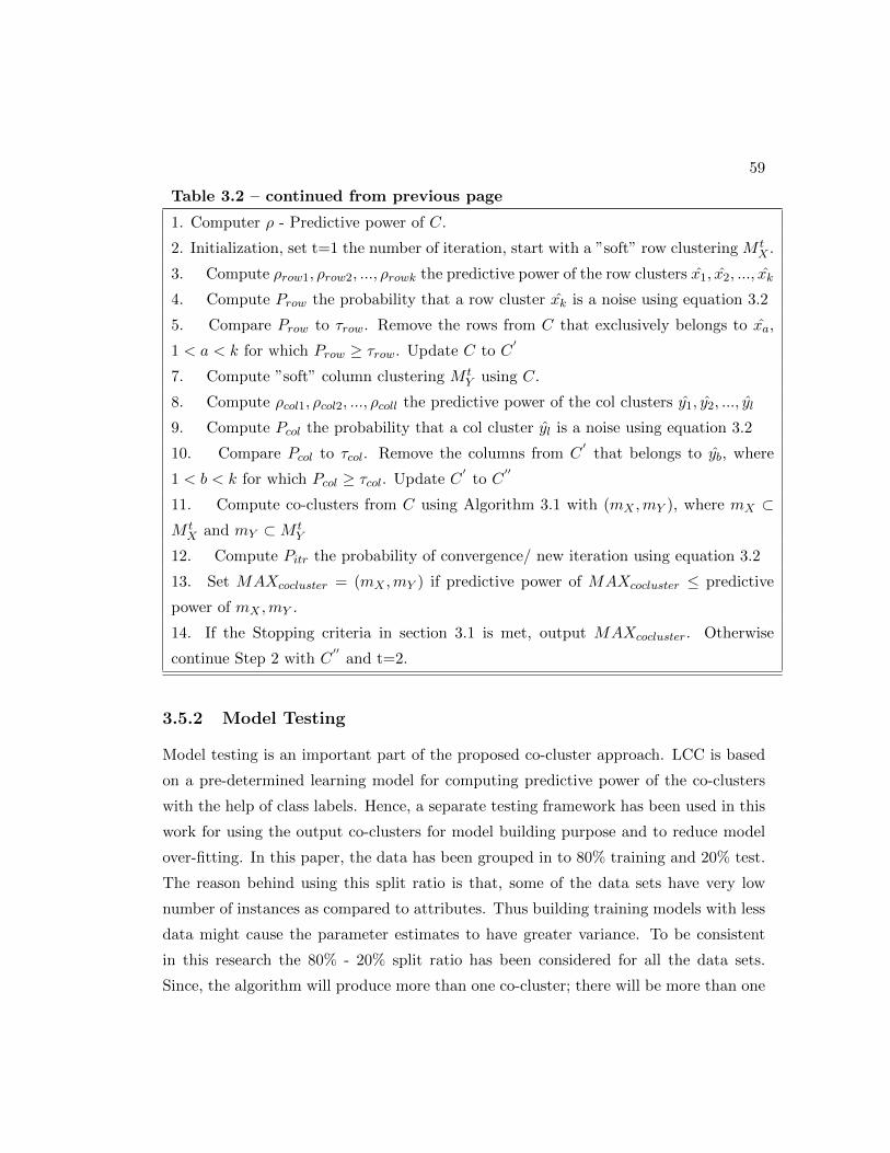
59
Table 3.2 – continued from previous page
1. Computer ρ - Predictive power of C.
2. Initialization, set t=1 the number of iteration, start with a ”soft” row clustering M tX .
3. Compute ρrow1, ρrow2, ..., ρrowk the predictive power of the row clusters x1, x2, ..., xk
4. Compute Prow the probability that a row cluster xk is a noise using equation 3.2
5. Compare Prow to τrow. Remove the rows from C that exclusively belongs to xa,
1 < a < k for which Prow ≥ τrow. Update C to C′
7. Compute ”soft” column clustering M tY using C.
8. Compute ρcol1, ρcol2, ..., ρcoll the predictive power of the col clusters y1, y2, ..., yl
9. Compute Pcol the probability that a col cluster yl is a noise using equation 3.2
10. Compare Pcol to τcol. Remove the columns from C′
that belongs to yb, where
1 < b < k for which Pcol ≥ τcol. Update C′
to C′′
11. Compute co-clusters from C using Algorithm 3.1 with (mX ,mY ), where mX ⊂M tX and mY ⊂M t
Y
12. Compute Pitr the probability of convergence/ new iteration using equation 3.2
13. Set MAXcocluster = (mX ,mY ) if predictive power of MAXcocluster ≤ predictive
power of mX ,mY .
14. If the Stopping criteria in section 3.1 is met, output MAXcocluster. Otherwise
continue Step 2 with C′′
and t=2.
3.5.2 Model Testing
Model testing is an important part of the proposed co-cluster approach. LCC is based
on a pre-determined learning model for computing predictive power of the co-clusters
with the help of class labels. Hence, a separate testing framework has been used in this
work for using the output co-clusters for model building purpose and to reduce model
over-fitting. In this paper, the data has been grouped in to 80% training and 20% test.
The reason behind using this split ratio is that, some of the data sets have very low
number of instances as compared to attributes. Thus building training models with less
data might cause the parameter estimates to have greater variance. To be consistent
in this research the 80% - 20% split ratio has been considered for all the data sets.
Since, the algorithm will produce more than one co-cluster; there will be more than one

60
learning models being trained on the co-clusters. For a given test instance, it is therefore
important to determine the most suitable learning model in which it should be tested.
For this purpose, a distance based model choosing criteria based on nearest neighbor
approach has been develped and shown in algorithm 3.3 and equation 3.3. It can be
assumed that a given test instances is closest to a co-cluster if the distance from the
test instance and the centroid of the co-cluster is minimum from among all the possible
co-clusters. Next, testable predictions has been computed with the chosen co-cluster
model.
Table 3.3: Calculate closest Co-Cluster
Algorithm
Input:co-clusters ci given 1 < i < c where c is the number of co-clusters, test instance t
Output: final selected co-cluster
Steps:
1. For i = 1 to c
2. Set a temporary variable MINdist = 10000.
3. Calculate centroids of ci according to definition 3
4. Calculate the distance between ci and t according to equation 3.3
5. IF MINdist > ci
6. then MINdist = ci
7. END IF
8. End For
9. Select Mindist from above
10. Output co-cluster with the Mindist
L =√
Σci=1(ti − µ)2 (3.3)
In the equation above L is the distance between the test instance t and the cluster
centroid µ. In this equation c is the number of co-clusters under consideration.
Definition 3 The centroid of a co-cluster can be defined as a data point where the
parameter values are the mean of the parameter values of all the data points in the

61
co-cluster.
In the following sections the results of LCC algorithm has been shown over five data
sets and compare them with two popular techniques known as Bayesian co-clustering
[72] and Spectral co-clustering [67]. As predictive power accuracy of Naive Bayes clas-
sification model has been used. Accuracy here refers to the percentage of correctly
classified instances. Results using J48 classifier and f-measure as the predictive power
has also been evaluated in this research.
3.5.3 Evaluation Metrics and Experimental Setup
In this work the quality of the co-clusters has been evaluated using accuracy, cluster-
precision, cluster-recall and cluster-f-measure. The measures cluster-precision, cluster-
recall and cluster-f-measure tries to estimate whether the prediction of each pair of
points that share at least one co-cluster, are in the same co-cluster and are correct with
respect to the underlying true groups or class labels in the data. Detail is given below -
• Classification accuracy - predictive power of the learning model built on the
final co-clusters computed with separate test instances. Naive Bayes as the clas-
sification algorithm has been used primarily in this work. A separate unseen test
instances (class labels of these instances are only used for validation purpose) has
been used for resulting co-cluster evaluation. Classification accuracy is calculated
as given in equation 3.4. In this work results with classification f-measure as the
predictive power has also been conducted to demonstrate that LCC is not limited
to using classification accuracy as its predictive power.
Accuracy =100 ∗No.ofCorrectlyClassifiedInstances
Totalno.ofinstances(3.4)
• Cluster-precision. Cluster-precision has been used for evaluating cluster quality
as defined in [16]. In the co-clustering results, cluster-precision is calculated as
the fraction of pairs of objects correctly put in the same co-cluster as given in
equation 3.5.
Precision =No.ofCorrectlyIdentifiedPairs
No.ofIdentifiedPairs(3.5)
62
• Cluster-recall Recall has been used for evaluating cluster quality as defined in
[16].Recall is calculated as the fraction of actual pair of objects that were identified
as given in equation 3.6.
Recall =NumberofCorrectlyIdentifiedpairs
NumberofTruepairs(3.6)
• Cluster-f-measure. It is the harmonic mean of precision and recall using equa-
tion 3.5 and 3.6 above. This can be calculated as given in equation 3.7.
F −measure =2 ∗ precision ∗ recallprecision+ recall
(3.7)
3.5.4 Data Set
Four data sets has been used namely AML data set [40], MovieLens data set [84],
Internet-Ads [36, 85], Madelon [85] as shown in table 3.4. Acute myelogenous leukemia
or AML is a real world data set that contains 246 demographic, genetic, and clinical
variables from 831 patients who received myeloablative, T-cell replete, unrelated donor
(URD) stem cell transplants [86, 87]. Internet-ads data set, represents a set of possible
advertisements on Internet pages. The features of this data set consists of the image
geometry, URL and text of the image, phrases occurring in the URL and words occurring
near the anchor text and the anchor text itself. The MovieLens data set [84], is a publicly
available data set used for movie recommendation systems developed by grouplens.org
in University of Minnesota. The MovieLens data set consisted of 100,000 movie ratings
by 943 users for 1673 movies. Each user rated the movies at a scale of 1-5, where 1
denotes extreme dislike and 5 denotes strong approval. Two genres has been chosen -
Action and drama movies rated by 943 users for 930 movies. Data sets are tabulated in
table 3.4. A consider binary class membership has been assumed with two class labels
for all data sets.
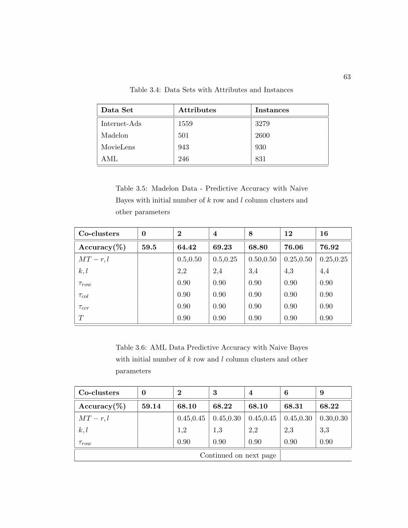
63
Table 3.4: Data Sets with Attributes and Instances
Data Set Attributes Instances
Internet-Ads 1559 3279
Madelon 501 2600
MovieLens 943 930
AML 246 831
Table 3.5: Madelon Data - Predictive Accuracy with Naive
Bayes with initial number of k row and l column clusters and
other parameters
Co-clusters 0 2 4 8 12 16
Accuracy(%) 59.5 64.42 69.23 68.80 76.06 76.92
MT − r, l 0.5,0.50 0.5,0.25 0.50,0.50 0.25,0.50 0.25,0.25
k, l 2,2 2,4 3,4 4,3 4,4
τrow 0.90 0.90 0.90 0.90 0.90
τcol 0.90 0.90 0.90 0.90 0.90
τccr 0.90 0.90 0.90 0.90 0.90
T 0.90 0.90 0.90 0.90 0.90
Table 3.6: AML Data Predictive Accuracy with Naive Bayes
with initial number of k row and l column clusters and other
parameters
Co-clusters 0 2 3 4 6 9
Accuracy(%) 59.14 68.10 68.22 68.10 68.31 68.22
MT − r, l 0.45,0.45 0.45,0.30 0.45,0.45 0.45,0.30 0.30,0.30
k, l 1,2 1,3 2,2 2,3 3,3
τrow 0.90 0.90 0.90 0.90 0.90
Continued on next page
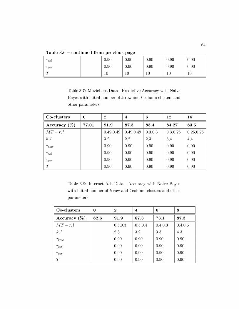
64
Table 3.6 – continued from previous page
τcol 0.90 0.90 0.90 0.90 0.90
τccr 0.90 0.90 0.90 0.90 0.90
T 10 10 10 10 10
Table 3.7: MovieLens Data - Predictive Accuracy with Naive
Bayes with initial number of k row and l column clusters and
other parameters
Co-clusters 0 2 4 6 12 16
Accuracy (%) 77.01 91.9 87.3 83.4 84.27 83.5
MT − r, l 0.49,0.49 0.49,0.49 0.3,0.3 0.3,0.25 0.25,0.25
k, l 3,2 2,2 2,3 3,4 4,4
τrow 0.90 0.90 0.90 0.90 0.90
τcol 0.90 0.90 0.90 0.90 0.90
τccr 0.90 0.90 0.90 0.90 0.90
T 0.90 0.90 0.90 0.90 0.90
Table 3.8: Internet Ads Data - Accuracy with Naive Bayes
with initial number of k row and l column clusters and other
parameters
Co-clusters 0 2 4 6 8
Accuracy (%) 82.6 91.9 87.3 73.1 87.3
MT − r, l 0.5,0.3 0.5,0.4 0.4,0.3 0.4,0.6
k, l 2,3 3,2 3,3 4,3
τrow 0.90 0.90 0.90 0.90
τcol 0.90 0.90 0.90 0.90
τccr 0.90 0.90 0.90 0.90
T 0.90 0.90 0.90 0.90

65
Table 3.9: AML Data - f-measure with J48 with initial num-
ber of k row and l column clusters and other parameters
Co-clusters 0 2 4 6 8 12
f-measure 0.61 0.93 0.76 0.75 0.75 0.74
MT − r, l 0.5,0.5 0.5,0.5 0.5,0.5 0.5,0.5 0.45,0.5
k, l 1,2 2,2 2,3 4,2 4,3
τrow 0.90 0.90 0.90 0.90 0.90
τcol 0.90 0.90 0.90 0.90 0.90
τccr 0.90 0.90 0.90 0.90 0.90
T 10 10 10 10 10
Table 3.10: AML Data - f-measure with Naive Bayes with
initial number of k row and l column clusters and other pa-
rameters
Co-clusters 0 2 4 6 8 10
F-measure (%) 0.53 0.59 0.56 0.72 0.71 0.71
MT − r, l 0.5,0.3 0.5,0.4 0.4,0.3 0.4,0.6 0.4,0.3
k, l 2,3 3,2 3,3 4,3 3,4
τrow 0.90 0.90 0.90 0.90 0.90
τcol 0.90 0.90 0.90 0.90 0.90
τccr 0.90 0.90 0.90 0.90 0.90
T 10 10 10 10 10
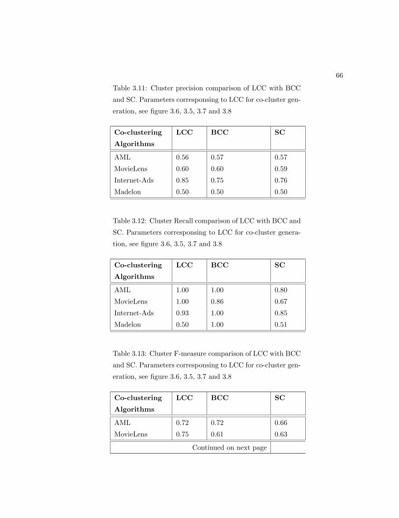
66
Table 3.11: Cluster precision comparison of LCC with BCC
and SC. Parameters corresponsing to LCC for co-cluster gen-
eration, see figure 3.6, 3.5, 3.7 and 3.8
Co-clustering
Algorithms
LCC BCC SC
AML 0.56 0.57 0.57
MovieLens 0.60 0.60 0.59
Internet-Ads 0.85 0.75 0.76
Madelon 0.50 0.50 0.50
Table 3.12: Cluster Recall comparison of LCC with BCC and
SC. Parameters corresponsing to LCC for co-cluster genera-
tion, see figure 3.6, 3.5, 3.7 and 3.8
Co-clustering
Algorithms
LCC BCC SC
AML 1.00 1.00 0.80
MovieLens 1.00 0.86 0.67
Internet-Ads 0.93 1.00 0.85
Madelon 0.50 1.00 0.51
Table 3.13: Cluster F-measure comparison of LCC with BCC
and SC. Parameters corresponsing to LCC for co-cluster gen-
eration, see figure 3.6, 3.5, 3.7 and 3.8
Co-clustering
Algorithms
LCC BCC SC
AML 0.72 0.72 0.66
MovieLens 0.75 0.61 0.63
Continued on next page

67
Table 3.13 – continued from previous page
Internet-Ads 0.89 0.86 0.85
Madelon 0.50 0.67 0.50
3.5.5 Results and Discussion
The performance of LCC has been compared with respect to the predictive power of the
co-clusters with the original data set. Naive Bayes classifiers has been considered as the
predictive power. Results with J48 classifier as well as f-measure as the predictive power
has also been presented in this work. The data set is split into 80% - 20% training and
test set respectively for all the data sets. In this work, the parameter setting with the
best result has been shown for a given data set. Parameter selection algorithm for LCC
can be extended as the future work.
In Tables 3.6 3.5, 3.8 and 3.7, the co-clustering result has been shown in terms
of classification accuracy with different number of co-clusters formed. Here, zero co-
clusters refer to the original data set. Result has been tested on two bench mark data
sets namely, madelon and Internet-Ads as well as two real world data sets namely,
AML and MovieLens. In AML data set the classification accuracy of Naive Bayes
model built on co-clusters are better than the original data set by more than 10%. In
madelon data set there is a significant improvement in the mean predictive power with
co-clustering. In MovieLens data set the classification accuracy increases by more than
8% from the actual data set. Lastly, Internet-Ads have significantly better classification
accuracy with smaller number of co-clusters than the original data set. It is important
to remember that the co-clusters are overlapping i.e. might have common instances or
features. Hence, in certain cases, accuracy might not vary a lot when the number of
co-clusters changes. From the above it is clear that the classification accuracy of Naive
Bayes model built on the co-clusters is better than the original data set. A different
variation of the proposed algorithm on the real world AML data set with f-measure
being used as the predictive power and J48 classifier has been presented next. Figure
3.10 and 3.9 shows that even when weighted f-measure has been used as the predictive
power, the overall result improves with LCC with Nave Bayes as well as decision tree.
This shows that LCC algorithm is robust towards the type of classification model used
68
for a given data set.
Next, the performance of the proposed algorithm with two state of the art co-
clustering method proposed in [72] by Shan et. al and [67] by Dhillon et. al has
been compared with LCC algorithm. In [72] Shan et. al proposed overlapping co-
clustering technique which maintains separate Dirichlet models for probability of row as
well as column clusters. In this paper a co-clustering algorithm has been developed by
modeling data matrix as a bipartite graph. In figure 3.5, the predictive power of LCC
has been compared with Bayesian co-clustering by [72] (let’s call it BCC) and Spectral
co-clustering by [67] (Let’s call it SC). Naive Bayes is the learning model and accuracy
of the model is the predictive power for evaluating (two and four) co-clusters generated
using each of the methods. From figure 3.5, it is clear that classification model built
using co-clusters generated with the proposed method is more accurate than the other
two methods for all the data sets. Now, predictive power for evaluating co-clusters
helps us understand the potential and usefulness of the proposed algorithm. However,
the evaluation might be incomplete if the purity of the co-clusters formed is not tested.
Three cluster evaluation techniques namely cluster-precision, cluster-recall and cluster-
f-measure as given in equation 3.5, 3.6 and 3.7 and defined by [16] has been used in
this work. In the experiments in this paper binary class labels has been used for all
the data sets. In binary class data, the binary class labels are the true class or ground
truth for evaluating cluster-precision and cluster-recall. From the figures 3.11, 3.12 and
3.13, It can be seen that AML dataset has same cluster-recall and cluster-f-measure as
BCC which is better than that of SC. In movieLens data, cluster-precision and cluster-
f-measure are better than that of both BCC and SC. In Internet-Ads data set all three
scores are significantly better than that of BCC and SC. Madelon data set produces the
three scores same as that of SC but lower than BCC. It should be noted that though the
three scores obtained using LCC for madelon is slightly low, they are not significantly
lower than BCC. The overall outcome of cluster-precision, cluster-recall and cluster-
f-measure suggest that in all the data sets LCC performs better than SC and BCC
(except madelon which is slightly lower than BCC). This proves that predictive power
of the co-clusters was augmented not at the cost of their purity. This shows that LCC
generates co-clusters with higher predictive power than the original data set as well as
preserves the purity of the actual co-clusters when compared with the true category of
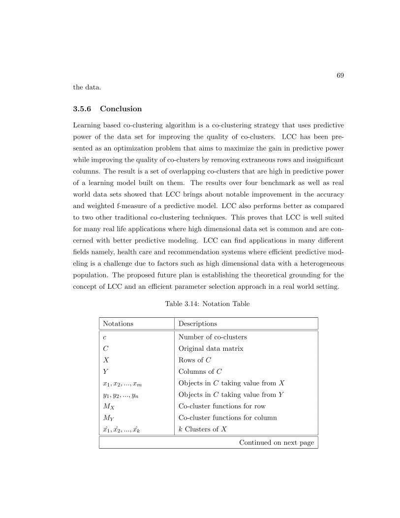
69
the data.
3.5.6 Conclusion
Learning based co-clustering algorithm is a co-clustering strategy that uses predictive
power of the data set for improving the quality of co-clusters. LCC has been pre-
sented as an optimization problem that aims to maximize the gain in predictive power
while improving the quality of co-clusters by removing extraneous rows and insignificant
columns. The result is a set of overlapping co-clusters that are high in predictive power
of a learning model built on them. The results over four benchmark as well as real
world data sets showed that LCC brings about notable improvement in the accuracy
and weighted f-measure of a predictive model. LCC also performs better as compared
to two other traditional co-clustering techniques. This proves that LCC is well suited
for many real life applications where high dimensional data set is common and are con-
cerned with better predictive modeling. LCC can find applications in many different
fields namely, health care and recommendation systems where efficient predictive mod-
eling is a challenge due to factors such as high dimensional data with a heterogeneous
population. The proposed future plan is establishing the theoretical grounding for the
concept of LCC and an efficient parameter selection approach in a real world setting.
Table 3.14: Notation Table
Notations Descriptions
c Number of co-clusters
C Original data matrix
X Rows of C
Y Columns of C
x1, x2, ..., xm Objects in C taking value from X
y1, y2, ..., yn Objects in C taking value from Y
MX Co-cluster functions for row
MY Co-cluster functions for column
x1, x2, ..., xk k Clusters of X
Continued on next page

70
Table 3.14 – continued from previous page
Acronym Meaning
y1, y2, ..., yl l Clusters of Y
F (.) Predictive power function
t′ Number of iteration
ρ Predictive power of C
∆ρ Gain in ρ from last iteration
ρrow1, ..., ρrowk Predictive power of each row cluster
ρcol1, ..., ρcoll Predictive power of each column cluster
τrow Threshold for row noise removal
τcol Threshold for column noise removal
Pitr Probability of iteration
Prow Probability of row noise removal
Pcol Probability of column noise removal
τccr Threshold for probability of Iteration
C ′ Data matrix after row noise removal
C ′′ Data matrix after column noise removal
3.6 Co-clustering in Medical Domain: Improving predic-
tion of Relapse in Acute Myelogeneous Leukemia Pa-
tients with a Supervised Co-clustering technique
In acute myelogenous leukaemia (AML) patients with blood related malignancies, the
standard treatment constitutes Allogeneic hematopoietic stem cell transplantation (HSCT)
using related or unrelated donors. Several patients can not be cured my chemotherapy
alone and the survival is limited by treatment related mortality and relapse. The suc-
cess or failure of HSCT is affected by various genetic factors such as tissue type or hu-
man leukocyte antigen (HLA) type and immune cell receptors, including the killer-cell
immunoglobulin-like receptor (KIR) family. One of the most important task constitutes
variables selection with informative interactions for an effective outcome prediction. In
71
this paper, a methodology for developing a supervised overlapping co-clustering tech-
nique technique has been proposed that will improve predictions of outcomes after
HSCT for AML patients. The proposed supervised co-clustering technique using HLA
and KIR genotype data, can efficiently assist in donor selection before HSCT and confer
significant survival benefit to the patients. In this work the co-clustering is proposed
as an optimization problem for a more effective and improved predictive analysis. The
proposed algorithm generates co-clusters by maximizing its predictive power subject to
constraints on the number of co-clusters. It has been shown with extensive empirical
evaluation with donor and host genotype as well as clinical characteristics that LCC
generates co-clusters that improves predictive power of learning model, as high as 10%
over the original data set. In this work, it has been shown that the proposed technique
has better performance than two state-of-the-art co-clustering methods namely, Spectral
Co-clustering and Bayesian Co-clustering. In this work, LCC has been evaluated using
two benchmark and two real world data sets. The results demonstrate the effectiveness
and utility of the proposed technique having great potential in the medical domain.
3.6.1 Introduction
Acute myeloid leukemia (AML), also known as acute myelogenous leukemia, is a cancer
of the myeloid line of blood cells, characterized by the rapid growth of abnormal white
blood cells that accumulate in the bone marrow and interfere with the production of
normal blood cells. AML is the most common acute leukemia affecting adults, and its
incidence increases with age. In the United States approximately, 12,000 cases of AML
are diagnosed. For many patients, chemotherapy is not the best treatment alone, and
require hematopoietic stem cell transplantation (HSCT)for curative therapy. While
HSCT can cure AML, it is a complex procedure with many factors influencing the
outcomes, which remain suboptimal [39]. For a successful allogeneic HSCT, the leukemia
cells must be eradicated by the, combined effect of chemotherapy, radiotherapy, and a
donor T cell mediated graft-versus-leukemia reaction. There are various factors such
as donor age, gender, parity, and prior exposure to viruses such as cytomegalovirusare
that can influence transplant outcomes [41]. Recently, in the investigation community,
focus has been on the role of natural killer (NK) cells on mediating beneficial effects in
HSCT [42], [41]. NK cells express polymorphic killer-cell immunoglobulinlike receptors
72
(KIR)[42], [43] which influence the function of NK cells which can kill leukemia cells,
decrease rates of graft versus host disease, and control infections after HSCT. Because
the HLA genes and KIR genes are on separate chromosomes only 25% of HLA-matched
sibling donors are KIR identical and unrelated HLA-matched donors are rarely KIR
identical [44]. Two papers analyzed a retrospective cohort of patients that received
unrelated donor transplants for AML and demonstrated the beneficial effect of certain
donor KIR genes on preventing relapse and improving survival after HSCT [41]. The
identification of groups of KIR genes from the centromeric and telomeric portions of
the genetic region which were associated with relapse protection and survival were one
of the most important results. Specifically, donors with KIR B haplotype genes were
found to be protective against the outcome relapse.
A critical part of the entire transplant procedure is developing a good donor selec-
tion strategy and past researches have looked into donor and host genetic factors that
can predict a successful outcome after transplantation. Statistical [41], [42], [43] as
well as data mining researches [3],[87] has shown that selection of significant variables
can greatly assist donor selection resulting in a successful HSCT. Detection of hidden
interaction between the donor and the recipient variables is another important factor
that needs much attention. This is because, this will enable medical experts to focus
on informative variables from among hundreds of variables available from the patients
and thus decrease the mortality rate in AML patients by improving outcome relapse
after HSCT. Due to the large size of the available data with hundreds of variables
and thousands of patients, this problem has attracted attention from the data mining
and machine learning community. Past researches in data mining in this area [3],[87]
has shown that significant outcome benefits are achievable using feature selection tech-
niques for prediction of relapse. The volume of the available data and the presence
of insignificant variables and extraneous data (missing values and wrongly recorded
patient information) can greatly limit the accuracy of predictive models built on the
data. Therefore, instead of building predictive models on data from a noisy domain,
homogeneous groups (i.e. groups of patients with similar characteristic pattern over
a subset of clinical and genetic variable) can be extracted from the data for building
more effective predictive models. Detection of these hidden groups can greatly assist in
improved predictions, capturing significant donor and host variable interactions as well

73
as discovering relationships between variables by affecting outcome relapse for patients.
In this thesis a novel supervised co-clustering algorithm has been developed called
that can improve prediction of relapse outcome after HSCT in AML patients. The key
idea of this algorithm is to generate optimal co-clusters by maximizing predictive power
of the co-clusters subject to the constraints on the number of co-clusters. The resulting
clusters are high in predictive power (for example classification accuracy, f-measure)
when a learning (classification) model is built on them. The proposed algorithm has
the added advantage that, co-clusters generated are overlapping in nature. Most impor-
tantly, there is no need to pre-specify the number of co-cluster as a parameter. Most of
the existing co-clustering algorithm focuses on finding co-clusters with single member-
ship of a data point in the data matrix [61]. Although these techniques generate efficient
results over real data set, these algorithms are based on the assumption that, a single
data point can belong to only one cluster. This assumption is often not completely valid
since, in real life there is a high probability that a single data point belongs to multiple
clusters with varying degree of its membership with the clusters. For example, a group
of AML patients undergoing HSCT can reflect sub-populations that potentially share
co-morbid diagnoses. Thus co-clustering can be a suitable approach for finding groups
of patients and disease conditions that will help capture the most utilizable pattern that
exists in the clinical information.
In co-cluster analysis, detecting good co-clusters is a non-trivial task. AML data is
high dimensional and consists of noise in the form of extraneous instances and insignifi-
cant features. Co-clusters extracted from these data might not be suitable for a specific
supervised learning purpose if these co-clusters have been obtained from a complete
unsupervised setting. In real life applications often predictive models are built on seg-
mented data using domain expert’s knowledge [64]. In such situation assigning a specific
supervised learning algorithm to a co-cluster becomes a challenge. In this research, a
co-clustering algorithm has been presented and a testing framework has been proposed
that removes noise from the data resulting in co clusters that improves the predictive
power of learning models built on them.
This algorithm has been defined as an optimal co-clustering that minimizes the
“loss” in predictive power (or maximizes the “gain” in predictive power). The goal
of this algorithm is to seek a “soft” clustering [65] of both dimensions such that the

74
“gain” in ”Predictive Power” of the co-clusters is maximized given an initial number of
row and column clusters. The number of co-cluster to be generated doesn’t need to be
pre-specified and is upper-bounded by maximum number of co-clusters to be generated
through an initial number of row and column clusters. It has been assumed that, class
information is available in a supervised setting for evaluating the predictive power of a
learning model built using co-clusters in the training phase.
The row clusters are generated by identification of a distinguished soft partition of
the data matrix in the row dimension such that data point belonging to a partition
has strong intra-object resemblance. The column clusters are generated in a similar
way. The optimal clustering criteria for a soft partition has been obtained using gen-
eralized least squared error functions [65]. The proposed algorithm is suitable for high
dimensional data because it reduces dimensions iteratively by removing noisy rows and
columns. The result of the proposed algorithm is a set of overlapping co-clusters with
reduced row and column noise and a higher predictive power than the original data.
The primary goal of developing a novel data mining based approach in this domain
is to identify homogeneous groups of relevant variables and patients because of the
complexity of HSCT and the high dimensional nature of the data. For evaluation the
predictive power of a learning model on the data has been built using the generated
co-clusters with that of the original data set.The performance is also compared with
two traditional co-clustering algorithms. Evaluation measures used are classification
accuracy, f-measure, cluster-precision, cluster-recall and cluster-f-measure calculated
over pairs of points. The main contributions of this work are -
1) In this work a co-clustering algorithm has been proposed that detects overlapping
homogeneous blocks of patients and informative variables that improves prediction
of relapse after HSCT in AML patients. An important property of this algorithm
is that there is no need to specify the number of co-clusters.
2) A separate model testing framework has been proposed with test patients for
reducing model over fitting and for a more accurate prediction of relapse.
4) LCC has been demonstrated with 927 AML patients and 212 clinical and genetic
variables set and show using empirical results that, the proposed approach yields
co-clusters that improves the predictive power of a learning model significantly for
75
predicting outcome relapse.
3.6.2 Related Work
Co-clustering techniques have immense potential to enhance data mining in the med-
ical domain as has been previously studied in areas such as predictive analysis using
feature selection [3],[87], medical image processing[45, 46, 47, 48]. Co-clustering tech-
niques are advantageous in medical domain because these enables us to group patients
/ samples and conditions or genes simultaneously, that is, the clustering is interde-
pendent. Another advantage of co-clustering is that in contrast to predictive analysis
on the whole data, predictive models built on co-clusters as homogeneous blocks may
give a better approximation of the closeness to the ground truth of a predictive model
[80]. Co-clustering techniques have been used in the past in the medical domain [88]
to diagnose heart disease and extract the underlying data pattern of the datasets. The
above technique is a probabilistic framework for model based co-clustering. To the best
of our knowledge, there is no other past work that developed a co-clustering exclusive
for improving prediction of relapse for AML patients in the medical domain. There are
very few works in the past, to the best of our knowledge that utilizes predictive power
of a data matrix to generate co-clusters. A recent work on semi supervised co-clustering
is by [79]. In this paper the authors finds optimal co-clustering by incorporating in
the clustering process, prior information regarding the existence of certain objects and
features. For this they use a matrix decomposition approach and solve co clustering
problem as a trace minimization problem. Another relevant work is by [80] where a
semi-supervised co-clustering technique has been developed that captures the inherent
structure of complex data and predicts missing entries by constructing simple local pre-
dictive models such as classification by regression. One drawback of this technique is
that the algorithm uses a divide and conquers strategy to find co-clusters by building
local predictive models. Therefore, when the number of co-clusters is large the prob-
ability of over fitting might increase. In contrast to the above mentioned works, this
algorithm is supervised in its training phase and in order to avoid over fitting, a separate
testing framework has been proposed that uses nearest neighbor based model selection
approach. The result is co-clusters that have greater predictive power than the original
data matrix as well it has less over fitting attributed by the separate testing framework.

76
The earliest works in co-clustering was done in 1972 using hierarchical row and col-
umn clustering in matrices by a local greedy splitting procedure [73]. In this paper, the
author proposed a hierarchical partition based two way clustering algorithm that splits
the original data matrix into set of sub-matrices and used variance for evaluating the
quality of each sub matrix. Later this method was improved by [74] that introduced a
backward pruning method for generating an optimal number of two way clusters. [62]
proposed a co-clustering algorithm that uses a mean squared residue as the measure
of the coherence of the genes and conditions for analysis of gene expression data. In
Information theory domain [75] proposed an approach called “Information bottleneck
theory” that was developed for one dimensional clustering. Later [61] extended their
work and proposed a co-clustering technique using the concepts of information theory.
Another important paper [67] proposed a co-clustering technique that was modeled
based on bi-partite graphs and their minimal cuts. Most of the works in the past have
focused on “crisp” or partition based co-clustering and very few recent research can
handle overlapping co-clusters [72]. Even for one-way clustering, there are few algo-
rithms known as “soft” clustering algorithms which can identify overlapping clusters.
One of the earliest example is fuzzy c-means clustering [65]. One of the notable works
in overlapping co-clustering was [16] where the authors have proposed an overlapping
co-clustering model that can be applied with a variety of clustering distance functions.
Other important works in overlapping co-clustering that has been shown to be of im-
mense utility in various fields includes [76], [77] and [78].
This data set has been chosen in part because it is high dimensional with missing
data, characteristic of real biologic data, and because it has been extensively studied
by traditional bio-statistical methods to provide good gold standard results to compare
to the findings. This data set is unique in that the donor and recipients of URD
HSCT were genotyped not only for their HLA alleles, but also for the NK receptor
KIR genes. It is known that the interactions between KIR and HLA molecules (their
natural ligands) affect the function of NK cells and their ablity to kill cancer cells
and to function to fight infection and promote overall immunity[42, 43, 51, 52, 53].
Several studies have documented the interaction between HLA and KIR on outcomes
after HSCT [54, 55, 56, 57]. The first study to demonstrate that both centromeric
and telomeric KIR genes from group B haplotypes contribute to relapse protection and
77
improved survival after URD HSCT for AML [41, 40] described this data set. The
authors identified genetic factors related to KIR that improve outcome after HSCT
by performing multivariate statistical analyses. The models included many donor and
recipient transplant and demographic variables known to affect the outcome of HSCT.
Research exists that previously published analyses of this data set. These works
designed a decision strategy to efficiently select the optimal donor to prevent relapse
after transplant and to improve survival. The methodologies used in these studies were
primarily to interpret a plethora of variables, based on prior knowledge using classical
statistical tests of hypotheses generated by physicians. However, this approach, while
highly accurate, is potentially limited by the biases of the researchers generating the
hypotheses and time consuming.
Treatment decisions for any medical condition can be challenging. The ultimate
decision especially in case of transplants, rest with the physicians, who may be over-
whelmed with a confusing range of information sources. The data is huge in medical
domain and human beings have a limited ability to retain information as compared to
the artificial intelligence, and this worsens when the amount of information increases.
For example in the AML data it is non-trivial to detect the interaction between specific
variables from donor and recipients, for deciding on the best donor selection strategy.
Determining if such an interaction can be harmful or beneficial for a HSCT procedure
is informative for an outcomes prediction. In such situations co-clustering can greatly
assist as an automated techniques that can identify homogeneous blocks of patients and
variables significant for predicting relapse. Using the proposed co-clustering algorithm,
interesting rules and relationships can be sought and discovered without the need for
prior knowledge. Data mining in general helps to capture cumulative experience of
all the patients reflected in the entire database which can exhibit unknown pattern of
medical significance. In this regard, co-clustering technique can prove to be a highly ef-
ficient approach for detecting the contributing groups of patients and variables from an
entire database. The result obtained is a set of highly significant variables and relevant
patient records which can be used for accurate prediction purpose, either using classifi-
cation techniques or statistical approaches. In this research the aim is to providing the
medical domain with a novel co-clustering approach which will help the domain experts
in donor selection for a successful HSCT outcome by improving the predictive power
78
of the learning model. In medical domains like HSCT, no research is known to have
been conducted to the best of our knowledge, using an efficient overlapping co-clustering
technique which can be utilized for successful prediction outcomes. This research can be
considered as the first known work in the development of a supervised co-clustering ap-
proach for improving prediction and a probable variable interaction detection strategy
for HSCT based on information obtained from a large clinical genotype data repository.
3.6.3 Supervised Co-clustering Algorithm
In this work, a supervised co-clustering algorithm has been proposed, that identifies
overlapping co-clusters from high dimensional AML data. This algorithm can be con-
sidered as a variant of two way co-clustering algorithms [82]. In two-way co-clustering,
separate one dimensional clustering is performed and the result is combined to generate
co-clusters. In this paper, the proposed algorithm generates one dimensional overlapping
clusters [65] from both row and column dimension and improves the co-clusters with an
objective function in successive iterations to find optimal overlapping co-clusters. The
one dimensional clusters are identified using two different scoring mechanisms namely
intra-cluster and inter-cluster distance. Instead of crisp allocation of data points to any
particular cluster, a membership matrix is generated which indicates the membership
of a data point in a single or more than one cluster [65]. An assumption made here is
a pre-defined membership threshold for the data points in both the dimensions. This
threshold allows allocation of data points to one or more than one cluster. After calcu-
lating overlapping clusters from both the dimensions, the co-clusters are optimized by
removing noisy rows and columns. This is continued in an iterative process until the
stopping criteria is met.
The motivation behind this approach is that, removing redundant or wrongly doc-
umented instances and irrelevant features from the data in form of noise, will assist
in improving the predictive power of a learning model built on the data. The statisti-
cal insights taken from these co-clusters would help effective predictive model building
and an improved decision making. For example, in recommendation systems, finding
user-item co-clusters from a heterogeneous population would help provide guidance for
predicting different genres of a movie for customers with similar interest.
LCC algorithm is interesting as it uses predictive power of the co-clusters to detect

79
and eliminate noisy rows and noisy columns while co-cluster formation. An added
advantage is that there is no need to specify the number of co-cluster. Most importantly,
this algorithm seeks to find overlapping or ”soft” co-clusters that might qualify it as an
algorithm that is closely capable of capturing the structure of real world data.
An iterative algorithm has been proposed in this work, with co-clusters getting re-
fined at iterations aided by the threshold of noise removal while maximizing the objective
function. The objective function is defined in equation 4 states that the algorithm aims
to maximize the predictive power of identified co-clusters, subject to the constraints on
the number of co-clusters c and 1 < c < k ∗ l, where k and l are the initial number
of row and column clusters. In equation 4, F (X; Y ) is the mean predictive power of a
model learned on the co-clusters generated in any given iterative stage. In general other
aggregate scores such as co-cluster with the the max or min predictive power can be
used. F (X;Y ) is the function that represents the predictive power of a learning model
on original data matrix (X;Y ). The gain in predictive power F (X; Y ) − F (X;Y ) can
be explained as the quantity that facilitates the search for an optimal co-clustering.
Definition 4 Learning based co-clustering can be defined as
Maximize(F (X; Y )− F (X;Y )) (3.8)
Subject to the constraints on the number of co-clusters c and 1 ≤ c ≤ k ∗ l, where k is
the initial no. of row cluster and l is the initial number of column cluster.
The co-clustering algorithm works as follows as given in algorithm 3.2. The stopping
criteria of the proposed algorithm assist in finding an approximately optimal solution.
This task is non-trivial since there is always a chance that the algorithm will end with
a local optimal solution. Therefore, a probabilistic neighborhood search approach has
been used namely, Simulated annealing [81] with a control parameter called cooling
schedule. This control parameter has been referred as T in the equation 3.2.
3.6.4 Experimental Evaluation
In the following section shows results of LCC algorithm over five data sets and compare
them with two popular techniques known as Bayesian co-clustering [72] and Spectral

80
co-clustering [67]. Classification accuracy of Naive Bayes classification model has been
used as predictive power. Accuracy here refers to the percentage of correctly classified
instances. Results using J48 classifier and f-measure has also been presented as the
predictive power.
3.6.5 Data set Properties
Acute myeloid leukemia or AML is a real world data set that contains 246 demographic,
genetic, and clinical variables from 831 patients who received myeloablative, T-cell re-
plete, unrelated donor (URD) stem cell transplants [40, 86, 87]. This data set consists of
1160 patients who received myeloablative, T-cellreplete, unrelated donor (URD) trans-
plantation as treatment for AML. Transplants were facilitated by the National Marrow
Donor Program (NMDP) between 1988 and 2006. DNA sample was obtained for each
donor and recipient from the Research Sample Repository of the NMDP. Outcome data
were obtained from the Center for International Blood and Marrow Transplant Research.
Complete highresolution HLA matching data at HLA-A, B, C, DRB1, and DQB1 were
obtained from the NMDP retrospective typing program. A total of 121 attributes were
studied. Gene expression data is binary (1- present and 0-absent). Response variable
considered was relapse along with other predictor variables such as KIR gene status
for donors as well recipients, HLA allele matching at A, B, C, DRB1, and DQB1, gen-
der and demographic information, karnofsky score (score that quantifies AML patients’
general well-being and activities of daily life), graft type and other genetic information.
Data Preprocessing
A preliminary domain based pruning was done on the data set to remove redundant
variables and missing values. Missing values could be interpreted in two ways- missing
at random and not missing at random. Certain numeric values corresponding to stan-
dard clinical measurements representing variables can be safely considered as missing
at random, since, we do not learn anything about the patient from the fact that these
particular measurements were not conducted. Hence, patients with such variables show-
ing empty fields were randomly assigned values within the variable range (estimated as
a Gaussian) from the rest of the patient population. On the other hand, the absence
of numeric values for certain variables can be considered approximately equivalent to

81
evidence of absence. That is, the most likely cause for the values being missing is that
the patients scores for these variables were held prima facie to be healthy, and hence,
were not measured. The recipient KIR genetic variables were removed since previous
analysis has demonstrated that they were not predictive of outcome after HSCT [40].
The final data contained 1160 instances and 69 attributes including KIR genes, HLA
allele matching at A, B, C, DRB1, and DQB1, age, race, sex, CMV status, graft type,
Karnofsky score, disease status before transplant. Response variables used for prediction
was relapse indicating whether the patient had a relapse of AML.
Evaluation
The quality of the co-clusters were evaluated using accuracy, cluster-precision, cluster-
recall and cluster-f-measure. Accuracy is the predictive power of the learning model built
on the data computed with separate test instances. Naive Bayes has been used as the
classification algorithm. A separate unseen test instances (class labels of these instances
are only used for validation purpose) has been used for resulting co-cluster evaluation.
This research also show results with classification f-measure (weighted harmonic mean
of precision/positive predictive value and recall/ sensitivity) as the predictive power
to demonstrate the fact that LCC is not limited to using classification accuracy as its
predictive power. The measures cluster-precision, cluster-recall and cluster-f-measure
are three different measures that have been inspired from the measures defined in [16].
These three measures tries to estimate whether the prediction of each pair of points that
share at least one co-cluster, are in the same co-cluster and are correct with respect to
the underlying true groups or class labels in the data. True groups has been assumed
to contain binary class labels for evaluating two co-clusters.
Classification Algorithms
In the following sections shows results of the proposed algorithm over AML data set
in terms of classification accuracy and f-measure and compare them with two popular
techniques known as Bayesian co-clustering [72] and Spectral co-clustering [67]. As
predictive power accuracy of Naive Bayes classification model has been used, using
estimator classes. Results using J48 classifier or pruned C4.5 decision tree has also been
showed in this work. Naive Bayes and Decision Tree has been chosen because these two

82
classification algorithms are the standard basic classifiers and it can be safely assumed
that an improved result indicates that LCC has the potential to work well with other
complex classifiers.
Figure 3.5: Comparison with BCC and SC
3.6.6 Results and Discussion
The mean predictive power of a learning model of the co-clusters is compared with
the original data set using LCC. Classification accuracy of Naive Bayes classifier is
considered to be the predictive power. Results with J48 classifier as well as f-measure
as the predictive power has been presented. The data set has been split into into 80%
- 20% training and test set respectively for all the data set. This work shows the
parameter setting chosen heuristically that gives the best result for a given data set. A
parameter selection algorithm can be extended as the future work.
Results for the AML data has been shown in table 3.10 , 3.6 and 3.9. In AML data
set the classification accuracy of Naive Bayes model built on co-clusters are better than
the original data set by more than 10%. From the above it is clear that the classification
accuracy of Naive Bayes model built on the co-clusters is better than the original data
set. A different variation of this algorithm on the real world AML data set has been
used with f-measure being used as the predictive power and J48 classifier. Table 3.10
and 3.9 shows that even when weighted f-measure has been used as the predictive power,
the overall result improves with LCC with Nave Bayes as well as decision tree. This
83
shows that LCC is robust towards the type of classification model used for a given data
set.
Next, the performance of LCC has been compared with two state of the art co-
clustering method proposed in [72] by Shan et. al and [67] by Dhillon et. al. In
[72] Shan et. al proposed overlapping co-clustering technique which maintains separate
Dirichlet models for probability of row as well as column clusters. In this paper a co-
clustering algorithm has been developed by modeling data matrix as a bipartite graph.
In figure 3.5, the predictive power of LCC with Bayesian co-clustering by [72] (BCC)
and Spectral co-clustering by [67] (SC) has been compared with LCC. Naive Bayes is
the learning model and accuracy of the model is the predictive power for evaluating (two
and four) co-clusters generated using each of the methods. From figure 3.5, it is clear
that classification model built using co-clusters generated with the proposed method
is more accurate than the other two methods for all the data sets. Now, predictive
power for evaluating co-clusters helps us understand the potential and usefulness of
the proposed algorithm. However, the evaluation might be incomplete if the purity
of the co-clusters is not tested. For this purpose, three cluster evaluation techniques
has been used namely cluster-precision, cluster-recall and cluster-f-measure as given in
equation 3.5, 3.6 and 3.7 and defined by [16]. In the experiments binary class labels
has been used for all the data sets. In binary class data, the binary class labels has
been considered as the true class or ground truth for evaluating cluster-precision and
cluster-recall. From the figures 3.11, 3.12 and 3.13, it can be seen that AML dataset
has same cluster-recall and cluster-f-measure as BCC which is better than that of SC.
In movieLens data, cluster-precision and cluster-f-measure are better than that of both
BCC and SC. In Internet-Ads data set all three scores are significantly better than that
of BCC and SC. Madelon data set produces the three scores same as that of SC but
lower than BCC. It should be noted that though the three scores obtained using LCC for
madelon is slightly low, they are not significantly lower than BCC. The overall outcome
of cluster-precision, cluster-recall and cluster-f-measure suggest that in all the data sets
LCC performs better than SC and BCC (except madelon which is slightly lower than
BCC). This proves that predictive power of the co-clusters was augmented not at the
cost of their purity. This shows that LCC generates co-clusters with higher predictive
power than the original data set as well as preserves the purity of the actual co-clusters
84
when compared with the true category of the data.
3.6.7 Conclusion
Learning based co-clustering algorithm is a co-clustering strategy that uses predictive
power of the data set for improving the quality of co-clusters. The novel algorithm
LCC has been presented as an optimization problem that aims to maximize the gain in
predictive power while improving the quality of co-clusters by removing extraneous rows
and insignificant columns. The result is a set of overlapping co-clusters that are high in
predictive power of a learning model built on them. The results over four benchmark
as well as real world data sets showed that LCC brings about notable improvement in
the accuracy and weighted f-measure of a predictive model. LCC also performs better
as compared to two other traditional co-clustering techniques. This proves that LCC is
well suited for many real life applications where one can handle high dimensional data
set and are concerned with better predictive modeling. LCC can find applications in
many different fields namely, healthcare and recommendation systems where efficient
predictive modeling is a challenge due to factors such as high dimensional data with a
heterogeneous population. The future plan for this work is establishing the theoretical
grounding for the concept of LCC and an efficient parameter selection approach in a
real world setting.

Chapter 4
Knowledge based missing value
imputation
Missing values in data is a very common problem in the real world due to reasons such
as manual data entry procedures, equipment errors and incorrect measurements. Prob-
lems associated with missing values are loss of efficiency, complications in handling and
analyzing the data and bias resulting from differences between missing and complete
data. In areas using data mining and machine learning techniques, missing values may
generate bias and affect the quality of the supervised learning process or the perfor-
mance of classification algorithm. But the quality of the data is major concern in any
field when building statistical and data mining models. In the domain of health-care,
data contains more than 1000 variables, which makes it highly sparse. In addition, this
data is incomplete, which makes most of the statistical and empirical analysis complex.
It is thus important to detect the factors that enhance or degrade the performance of
a clinical decision support system due to the high-dimensional sparse nature of health
care and medical data. Missing value imputation is an efficient way to estimate a prob-
able values based on available information in the data sets. Missing value imputation
methods encompasses a wide variety of techniques for imputation based on interesting
information in the data sets. Missing value imputation techniques can be of many differ-
ent types namely, using most common value, mean or median, closest fit approach and
methods based on data mining algorithms like k-nearest neighbor, neural networks and
85

86
association rules. All these techniques are based on information from within the data.
In the past domain expert has been involved in the missing value estimation process by
manually imputing values from their knowledge. However, this process is tedious and
almost impossible in huge data sets which is very common in today’s world. Presence
of huge volumes of data with thousands of dimension, missing value imputation replies
heavily on statistical analysis of the data and automated data mining techniques. In
these complex and efficient techniques, expert’s knowledge is included in rare cases. In
this research, a missing value imputation technique has been developed that is based
on both domain expert’s knowledge and statistical analysis of the available data. The
domain of HSCT has been chosen for case study and a group of stem cell transplant
physician’s opinion has been considered as the domain expert’s knowledge. The machine
learning approach developed can be defined as - rule mining with expert knowledge and
data analysis for missing value estimation. This technique was evaluated and the find-
ings were validated with two traditional evaluation measure on real world AML data
sets. This technique is compared with several other missing value imputation tech-
niques namely multiple imputation, KnnImpute [89], FIMUS [90], Median imputation
and random features.
4.1 Introduction
The health care data are usually in the form of large matrices of patient records (rows)
under different clinical conditions or variables (columns) describing some measure. This
data frequently contains values missing. Missing values occur for diverse reasons, in-
cluding insufficient or imprecise information provided by the patient, data corruption,
or simply due to wrong manual or systemic entry. Another Missing data may also oc-
cur systematically as a result of the robotic methods used to create them, for example
a faulty device. Such incomplete data is usually manually flagged and excluded from
subsequent analysis. However, this a may result in loss of valuable information for
future predictive analysis. Many analysis methods, such as principle components anal-
ysis or singular value decomposition, require complete matrices [91], [92]. Analysis of
data from health care and medical systems is challenging for a variety of reasons. The
data is generally very high-dimensional making it sparse and incomplete (that is, many
87
features describe patients but most of them are typically absent for any given patient)
[93]. The features are heterogeneous, encompassing quantitative data, categorical data
and text. Furthermore, these data are subject to random errors and systematic biases.
The traditional method of turning data into knowledge relies on manual analysis and
interpretation. For example, in the health-care industry, the specialists most of the
time analyze current trends and changes in health-care data on a periodic basis. They
provide a report describing the investigation to the sponsoring health-care organization
in order to use the report as the basis for imputing missing information, future decision
making and planning for health-care management [94]. However, such manual probing
of a dataset is slow, expensive, and highly subjective. This type of manual analysis
is slowly becoming impractical especially in health-care domains as data volumes grow
exponentially. This is where machine learning and data mining techniques prove to
be extremely useful [95]. Knowledge extraction from large databases using machine
learning techniques involves many steps, ranging from data manipulation and retrieval
to fundamental mathematical and statistical inference, search, and reasoning. In order
to approximate the underlying reality in data sets, it is necessary to discard various
artifacts, such as noise and fluctuations that occur through the acquisition and nor-
malization of data. Suspicious values are usually regarded as missing values, because
they may be detrimental to analyses further. There are several simple ways to deal
with missing values such as deleting an the data vector with missing values from further
analysis, imputing missing values to zero, or imputing missing values of a certain row
to the average [96]. Some researchers categorizes missing data into different categories
depending on how the actual data was generated [97]. They are
• If the probability of missingness is same for all the missing units, then the variable
defined to be missing completely at random. In this case discarding rows or column
corresponding to missing values does not bias the inferences.
• The missing value scenario is called Missing at Random which is different from
missing completely at random. This is a more general assumption, which states
that the probability a variable is missing depends only on available information.
Logistic regression is a common approach for modeling such situations, where the
outcome variable equals 1 for observed cases and 0 for missing.

88
• Situations where missingness is no longer at random; for example, the information
that has not been recorded and this information also predicts the missing values.
For example, a hypothetical situation can be that a patients with a heart disease
are less likely to be prescribed a kidney dialysis, having a heart condition is pre-
dictive of not requiring a kidney dialysis. In this case, kidney dialysis information
is not missing at random.
• Missingness can depend on the missing value itself. For example, in certain situa-
tions, patients with psychological disorders are less likely to provide any informa-
tion about their social habits for example, smoking habits and drug abuse.
Healh care integrates heterogeneous data from many sources, which is important for
knowledge discovery. The complexity, sparseness and fast evolution of clinical informa-
tion makes development, maintenance of clinical databases [98] and knowledge discovery
challenging. Health-care data are mostly sparse due to the high-dimensionality, i.e. the
data set contains a small amount of all possible values. Moreover, this data is incom-
plete i.e. each entity will have thousands of attributes, but each row in the table will
use only small set of these attributes as patient tests. Figure 4.1 shows a typical ex-
ample. Sparseness and incompleteness is one of the important challenges in health-care
data that past researches have recognized [99, 100]. Data incompleteness and sparseness
arises because doctors only perform a few different clinical lab tests among thousands
of test attributes for a patient over his lifetime. This property creates statistical as well
as empirical problems which reduce the efficiency and accuracy of any statistical tech-
niques for prediction purposes. It is therefore important to investigate the contributing
factors in the performance of a classification technique for prediction of PPE. The main
logic behind the data incompleteness problem is simple ; the basic probability theory
tells us that the probability of some complex event is the product of its independent
sub-events. Thus probability of some field in EHR data is the product of the conditional
probabilities of its component n fields for a single patient. Hence, if any of these n-field
has a zero probability , then the entire probability will be zero. This makes any kind of
probabilistic or statistical deduction such as Naive Bayes error prone.
The problem of missing values can be managed in many different ways from re-
peating the experiment or test, although this is often not feasible for economic reasons.
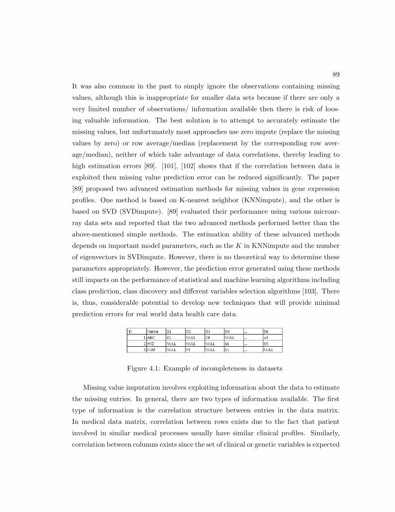
89
It was also common in the past to simply ignore the observations containing missing
values, although this is inappropriate for smaller data sets because if there are only a
very limited number of observations/ information available then there is risk of loos-
ing valuable information. The best solution is to attempt to accurately estimate the
missing values, but unfortunately most approaches use zero impute (replace the missing
values by zero) or row average/median (replacement by the corresponding row aver-
age/median), neither of which take advantage of data correlations, thereby leading to
high estimation errors [89]. [101], [102] shows that if the correlation between data is
exploited then missing value prediction error can be reduced significantly. The paper
[89] proposed two advanced estimation methods for missing values in gene expression
profiles. One method is based on K-nearest neighbor (KNNimpute), and the other is
based on SVD (SVDimpute). [89] evaluated their performance using various microar-
ray data sets and reported that the two advanced methods performed better than the
above-mentioned simple methods. The estimation ability of these advanced methods
depends on important model parameters, such as the K in KNNimpute and the number
of eigenvectors in SVDimpute. However, there is no theoretical way to determine these
parameters appropriately. However, the prediction error generated using these methods
still impacts on the performance of statistical and machine learning algorithms including
class prediction, class discovery and different variables selection algorithms [103]. There
is, thus, considerable potential to develop new techniques that will provide minimal
prediction errors for real world data health care data.
Figure 4.1: Example of incompleteness in datasets
Missing value imputation involves exploiting information about the data to estimate
the missing entries. In general, there are two types of information available. The first
type of information is the correlation structure between entries in the data matrix.
In medical data matrix, correlation between rows exists due to the fact that patient
involved in similar medical processes usually have similar clinical profiles. Similarly,
correlation between columns exists since the set of clinical or genetic variables is expected

90
to show similar pattern under similar conditions. Hence, it is possible to estimate the
missing entries based on subset of related patients or subset of related conditions. The
second type of information is domain knowledge about the data or the processes that
generate the data. The domain knowledge can be used to regularize the estimation such
that more plausible estimates are obtained. In this case, the imputation accuracy can
be increased by incorporating information about the underlying biological process or
the medical phenomena which would enhance the process of constraining the solution
to the missing value imputation problem. In this thesis, a missing value imputation
technique has been developed that utilizes domain expert’s knowledge and statistical
information from the data in order to enhance the performance of predictive models on
large data sets. The primary contributions of this work in this thesis are -
• A novel missing value imputation technique has been proposed, that utilizes both
domain expert’s knowledge as well as statistical information from the data such
as correlation and similarity among the variables.
• It has been shown that the proposed missing value imputation algorithm performs
better, when compared with other traditional missing value imputation techniques
with various percentage of missing values.
• Two different traditional evaluation measures has been used such as root mean
square error (RMSE) and Index of agreement to prove the effectiveness and utility
of the proposed missing value imputation technique.
• Results shows that the proposed missing value imputation technique can be effi-
ciently utilized in the domain of HSCT by applying the proposed technique in the
acute myelogeneous leukemia patient data set.
• This research shows that domain expert’s knowledge can enhance predictive mod-
eling especially in the medical domain with statistical knowledge from the data in
order to estimate missing values in high dimensional and sparse health care data
sets.

91
4.2 Related Work
Missing value imputation techniques can be categorized into many different categories.
Popular missing value imputation techniques includes imputation using predictive mod-
els [104], Bayesian network based missing value imputation [105], similarity analysis [90],
Rule based imputation [106] and clustering based imputation [107]. In [104] each es-
timate for missing values is attained by constructing a single regression model of the
target gene by a similar gene. This technique take the advantage of the correlation
structure in the microarray data and select similar genes for the target gene by Pearson
correlation coefficients. The above method also incorporates the least squares principle,
utilize a shrinkage estimation approach to adjust the coefficients of the regression model,
and then use the new coefficients to estimate missing values. In [105] the authors pro-
posed two imputation methods based on Bayesian networks in order to tackle missing
value imputation problem in classification task. In the first method, they constructs one
Bayesian network for each attribute with missing values, whereas the second method
uses a single Bayesian network for imputation in all attributes with missing values. The
authors in their paper has also elaborated on the bias inserted by imputation methods.
[90] uses data set’s existing patterns including co-appearances of attribute values, cor-
relations among the attributes and similarity of values belonging to an attribute. In the
paper [106], the authors develops a decision tree and expectation maximization (EM)
algorithm that can handle both numerical and categorical variables. In [107] the authors
develop a technique that imputes the missing values using a kernel-based method. The
authors fill up the missing values of an instance with those plausible values that are
generated from the data similar to this instance using a kernel-based random method.
Specifically, they first divide the data set into clusters. And then each of those instances
with missing-values is assigned to a cluster most similar to it. Finally, missing values of
an instance are estimated using a kernel-based method from the chosen cluster.
The paper [108] differentiated missing value imputation techniques for gene expres-
sion data based on the type of information used in the algorithm and named them as
global, local, hybrid and knowledge assisted. In Global category, algorithms perform
missing value imputation based on global correlation information derived from the en-
tire data matrix. They assume the existence of a global covariance structure among

92
all records or samples in the data matrix. One such example is the SVDImpute by
[89]. Algorithms in the local category exploit only local similarity structure in the data
set for missing value imputation. Only a subset of genes that exhibits high correlation
with the gene containing the missing values is used to compute the missing values in
the gene. Some of the earliest and well-known local imputation algorithms, such as,
K nearest-neighbor imputation (KNNimpute)[89] , least square imputation (LSimpute)
[102], local least square imputation (LLSimpute) [109], are some common examples.
KNNimpute [89] is perhaps one of the earliest and most frequently used missing value
imputation algorithms. KNNimpute uses pairwise information between the target gene
with missing values and the K nearest reference genes to impute the missing values.
The missing value in the target gene is estimated as the weighted average of the specific
component of the K reference genes. The weights are set to be proportional to the in-
verse of the Euclidean distance between the target and the reference genes. KNNimpute
performs well when strong local correlation exists between genes in the data. Several
modifications to the basic KNNimpute algorithm have been proposed [110], [111].
In the hybrid approach, the correlation structure in the data affects the performance
of imputation algorithms. If the data set is heterogeneous, local correlation between
genes are dominant and localized imputation algorithms such as KNNimpute or LL-
Simpute perform better than global imputation methods such as BPCA or SVDimpute.
On the other hand, if the data set is more homogenous, a global approach such as BPCA
or SVDimpute would better capture the global correlation information in the data. In
[112], the authors proposes a hybrid approach called LinCmb that captures both global
and local correlation information in the data. In LinCmb, the missing values are esti-
mated by a convex combination of the estimates of five different imputation methods:
row average, KNNimpute, SVDimpute, BPCA and GMCimpute. Row average, KNNim-
pute and GMCimpute uses local correlation information in their imputation, whereas
SVDimpute and BPCA uses global correlation information in their imputation. To
obtain the optimal set of weights that combine the five estimates, LinCmb generates
fake missing entries at positions where the true values are known and uses the con-
stituent methods to estimate the fake missing entries. The weights are then obtained
by performing a least square regression on the estimated fake missing entries. The final
weights for LinCmb are obtained by averaging the weights obtained in a pre specified

93
number of iterations.
In the category of knowledge assisted approach, domain knowledge is integrated
along with external information into the imputation process. The use of domain knowl-
edge has the potential to significantly improve the imputation accuracy beyond what is
possible with purely data-driven approach, especially for data sets with small number of
samples, noisy, or with high missing rate. Algorithms in this category can make use of,
for example, knowledge about the biological process in the microarray experiment [113],
knowledge about the underlying biomolecular process as annotated in Gene Ontology
(GO) [114], knowledge about the regulatory mechanism [115], information about spot
quality in the microarray experiment [116], and information from multiple external data
sets [117].
In this work,a strategy with similar motivation has been developed for missing value
imputation based on expert’s opinion. As a case study the domain of HSCT has been
chosen and a group of stem cell transplant physicians as the domain experts. This
work aims to estimate missing values from acute myelogeneous leukemia (AML) data
set where the data corresponds to AML patients undergoing Hematopoietic stem cell
transplantation (HSCT) also called bone marrow transplantation. The patient variables
constitutes genetic, clinical and demographic information for the patients as well as their
donor. In this approach an expert’s opinion has been combined with various statistical
information from the data and calculate an approximate value for the missing case. The
score calculation of the proposed approach has been adopted from[90] where the authors
calculates score based on all the non-missing entries of the data set. In the next section,
the following has been described - the problem statement, an intuition of this proposed
approach, methodology and results and discussion of findings from this research.
4.3 Problem Definition
In a typical data matrix, the rows are records from certain transaction or unique in-
formation under investigation, for example in AML data each individual data record
represents a patient undergoing HSCT. The columns on the other hand are the variables
representing a measure/ information regarding certain condition or time points; for ex-
ample in AML data each column represents genetic information (for a particular gene)
94
, clinical information or demographic information for all the patients. In general the
patient variable data matrix is obtained by performing a series of tests and observations
on the same set of patients, one for each column. Let the data matrix be represented as
an M X N matrix X where the entries of X are the variable information for M patients
with N different conditions. Then the element xij denotes the variable information
of the ith patient in the jth experiment. The objective of missing value imputation is
to estimate yij an estimate for xij , if xij is a missing entry given the incomplete data
matrix X.
In this work, the problem statement can be defined as - estimating yij using incom-
plete data matrix X and the domain expert’s knowledge E. The end result is such that
it the learning task of a predictive model built in the data set is improved. It is assumed
that the availability of class labels for all X in the training phase.
4.4 Methodology
The domain expert’s knowledge has been integrated with statistical information using
rules and then this information has been used to calculate scores. These scores are
calculated using information from domain expert’s knowledge and available data in the
form of similarity and correlation between variables selected by the domain experts and
the rules. This calculated score can be used to determine the probability of a possible
value to belong to the missing entry. The values for all the missing entry in the data
set is estimated. The technique is evaluated using RMSE and index of agreement which
denotes data resemblance between the variables. In the next sections, the methodology
has been described in great detail.
4.4.1 Expert’s Knowledge Based Missing Value Imputation
This thesis presents, expert’s Knowledge based Missing Value Imputation or EKMVI, a
missing value estimation technique that utilizes the knowledge from the domain experts
in estimating missing values in large data sets. The motivation behind this approach
is that, in most of the missing value imputation techniques, the information from the
existing data set is used. No prior knowledge is utilized. As a result the accuracy
of the future data analysis depends on the quality of imputation done using only the
95
incomplete data. On the other hand, in most of the previous data imputation techniques,
domain knowledge has been used as manual imputation by the domain experts. This
is in-feasible in the current scenarios where data is huge and manual imputation is
impossible. If data imputation is conducted using domain knowledge integrated with
the statistical measures from data, any data analysis task such as future predictions can
produce results that is closer to the ground truth.
EKMVI algorithm is interesting as it uses domain expert’s knowledge at first as raw
information and then converts it into useful rules. These extracted rules helps in de-
termining the variables significant in analyzing data for missing value estimation. Data
analysis for missing value estimation involves calculating scores for probable values for
imputation assuming only categorical variables are handled. These scores are calculated
based on similarity and correlation between variables from the variables extracted with
the help of rules. Numerical variables can also be handled by this proposed technique
by appropriately transforming the numerical variable into categorical variables.The final
score is compared and chosen value is imputed.
This research proposes to develop EKMVI as an score based missing value impu-
tation technique. The process of Knowledge based missing value imputation technique
consists of the following steps: 1) Knowledge collection from the experts 2) Integrating
knowledge into rules 3) Calculate scores 4) Using score for data imputation The entire
process of expert’s knowledge based missing value imputation is documented inside the
dotted box in figure 4.2. A more detailed view of this technique has been presented in
the figure 4.3.
4.4.2 Knowledge Collection From Experts
Knowledge from the experts can be collected and used in a variety of forms. They
can be ontologies, relationships and rules generated by the expert’s, from their prior
domain knowledge. In this work, simple knowledge has been used, for example - in the
domain of HSCT, a knowledge can be of the form ”Donor with full HLA match showed
an improved outcome of relapse”.
Let us now, briefly describe the domain of HSCT specifically acute myelogenous
leukemia (AML) in order to exemplify domain expert’s knowledge from AML per-
spective. Acute myelogenous leukemia (AML) is a blood related disease that require

96
Figure 4.2: Flow diagram of the expert’s knowledge based missing value imputationtechnique.
hematopoietic stem cell transplantation (HSCT) as one of the curative therapies from a
related or unrelated donor. Apart from Donor age, gender, parity, and prior exposure to
viruses such as cytomegalovirus, investigators have focused on the role of natural killer
(NK) cells on mediating beneficial effects in HSCT [40] . NK cells express polymorphic
killer-cell immunoglobulin like receptors (KIR) [41], which influence the function of NK
cells which can kill leukemia cells and control infections after HSCT.
In this work domain knowledge was collected from the experts in the form of variables
that are significant for the prediction of relapse of leukemia in AML patients after HSCT.
These features or variables has been deemed and proved to be significant by the experts
in the past who considers them as important for prediction of relapse [41]. In this
research, the variables suggested as significant are
• Donor−Final−Grp−ABx - variable differentiating between donor KIR genotype
group A/A (two A KIR haplotypes) and B/x (at least 1 B haplotype)
• Donor−Neutral−Better−Best - variable describing ‘neutral’, ‘better’ or ‘best’

97
groups based on number of centromeric and telomeric B-motifs [41]
• numhlaof10 - Variable describing Number of matches out of 10 based on HLA-A,
-B, -C, -DRB1 and -DQB1 [41]
• regigp - Conditioning regimen by group namely, Traditional myeloablative, Re-
duced Intensity, non-myeloablative, Non-traditional myeloablative and all others.
• disstat - Variables describing stages of disease at transplant namely, Early, Inter-
mediate, Advanced and others
• numtx - variable describing the total number of transplants the recipient (AML
patient) has had.
• leuk2 - variable that indicates wheher it is a secondary AML case or not.
• indxtx - variable describing interval from diagnosis to transplant (in months).
• karnofpr - The Karnofsky Performance Scale Index allows patients to be classified
as to their functional impairment. This can be used to compare effectiveness of
therapies such as HSCT and to assess the prognosis in individual patients. The
lower the Karnofsky score, the worse the survival for most serious illnesses [118].
4.4.3 Integrating Knowledge With Rules
Integrating the knowledge from the experts is non-trivial. The main challenge is the fact
that this knowledge should be converted and assimilated in an interpretative manner
without creating any kind of bias.
This research constitutes the strategies that can be described as follows - At first
perform association rule mining with data set with a user specified support and con-
fidence (0.2 has been used as support in this work). All variables that can be found
associated with V in the rules has been deboted as V ′. The score is calculated for
imputation using V and V ′. The steps taken in this work are as follows -
• Find all possible rules with a user specified support and confidence.
• For each attribute L where LεV , Find attributes V ′ from the rule R with an-
tecedent AR and consequent CR such that L = AR or L = CR.

98
Figure 4.3: Integrating knowledge into rules
• Select attributes V ′ and V for score calculation as the next step.
To find all possible rules an association rule mining namely, fpgrowth [119] has been
used on the dataset using the categorical variables. Mining association rules is a popu-
lar and well researched method for discovering interesting relations between variables in
large databases. PiatetskyShapiro [17] describes analyzing and presenting strong rules
discovered in databases using different measures of interestingness. Formally, the prob-
lem of mining association rules from transaction data can be stated as follows [120]. Let
I = i1, i2, ..., in be a set of n binary attributes called items. Let D = t1, t2, ..., tm be a
set of transactions called the database. Each transaction in D has a unique transaction
ID and contains a subset of the items in I. A rule is defined as an implication of the
form XY where X, Y I and XY = . The sets of items (for short itemsets) X and Y are
called antecedent (left-hand-side or LHS) and consequent (right-hand-side or RHS) of
the rule, respectively.
Using each antecedent (variables) that has been found to be associated with the
consequent (variable that has a missing value), scores are generated for estimating the
missing field as has been described in the next section.
99
4.4.4 Calculate Scores
This method of score calculation has been introduced in [90]. In this work, the score
calculation technique has been modified to include expert opinion. Let V variables from
the expert and V ′ is the other associated variables extracted from association rule in
the previous section. It can be assumed that typically a data set P maintains some
natural patterns in it. For example, the possibility of the appearance of a value Xij in
a record Xi depends on the other values of the record. The estimation for all possible
imputation values can be done by studying the co-appearance matrix C generated from
the variables V and V ′. An element cjk of the matrix C where cjkεC presents the total
number of co-appearances, from among union of variables V and V ′, between a pair of
values pεVj and kεVp belonging to two given attributes. Let fk be the frequency of k. It
can be observed that a high cjk/fk value indicates a high possibility of the appearance
of a value p given the appearance of the other value k. Let us denote the correlation
CorrV j,V k; ∀k between two attributes Vj and Vp. The correlation between attributes
are also taken into consideration since the attribute having high correlation should have
high influence in imputing the missing value.
let us assume that for a record Xi there is a missing value for the attribute Vj
having a domain i.e. range of possible values as (j1, j2, j3), and an available value k for
another attribute Vk with a domain (k1, k2, k3) i.e. Xij is missing and Xik = k1. The
co-appearance of j1 and k1; j1 and k2, and j1 and k3 has been calculated in order to
estimate the possibility of j1 being the correct imputation. Similarly the influence of
j2 and j3 are weighted according to their similarity with k1, k2 and k3. Next, the basic
concepts of this score computation technique has been described - with an example as
follows. Let the record Xi has a missing value in attribute VjεV , i.e. Xij is missing.
Let k1 be the actual value in the kth attribute VkεV , i.e. Xik = k1. Let Vj = j1, j2, j3
and therefore, j1, j2 and j3 are the candidates for possible imputation. Now a voting
system is used, where the best candidate having the highest vote is finally chosen as the
imputed value. Let, Cjk be the co-appearance of j and k in the V and V ′, and fk be
the total number of appearances (frequency) of k in the attributes V and V ′. ScoreN,pj1
is the vote in favor of j1 based on Vk considering only the available value k1. ScoreN,pj1
can be calculated as follows
ScoreN,pj1= Cjk/fk (4.1)
100
ScoreV S,pj1
is the vote in favor of j1 based on Vk considering the available value along
with its similar values. That is, ScoreS,pj1 is calculated considering k1, k2 and k3 as
follows.
ScoreS,pj1 = Σ∀vεVkCja/fa × Spk1a
(4.2)
where Spk1a is the similarity between k1(Xik = k1) and a of the kth attribute. Simi-
larity Spk1a is computed using an existing technique [121]. Then the weighted vote V k1j1
in favor of j1 based on attribute Vk as follow -
Scorepj1 = {ScoreN,pj1× λ+ ScoreS,pj1 × (1− λ)} ∗ Corrj1k1 (4.3)
where Corrjk is the correlation between the jth and the kth attributes. The Cramer’s
contingency coefficient [122] has been used to get correlation values between two at-
tributes. The values of the Cramer’s contingency coefficient vary between 0 and 1,
where a high value indicates a strong correlation. In the above equation, λ is a pa-
rameter value and the value for λ is 0.2 in this research. It has been shown in [90]
that 0.2 is an optimum value for this parameter. Next the total vote is calculate as
ScoreTj1 in favor of j1 by considering all attributes (V = V1, V2, ...Vl) and V ′ except the
jth attribute where l is the total number of significant variables suggested by experts
(since j εVj).This total vote is calculated as follows.
ScoreTj1 = Σ∀VkεV \VjScorekj1 (4.4)
Similarly, scores for ScoreTj2 and ScoreTj3 is calculated. Finally, the score having the
maximum value is considered to be the imputed value Xij .
4.4.5 Using Scores For Data Imputation
The score calculated above is used for imputing the missing value. Let Yij is the es-
timated value for imputing missing value for Xij then Yij = j1 with ScoreTa where
ScoreTa = Max(ScoreTj1 , ScoreTj2 , Score
Tj3); (4.5)
where ScoreTj1 , ScoreTj2 and ScoreTj3 are total scores as calculated in the previous
section.

101
Table 4.1: Missing value imputation Algorithm
Algorithm
Input: Expert’s knowledge E, where E = v1, v2, ...vl and lεV , V εE, Data set P
Output: Complete Data set P
Steps:
1. Perform association rule mining with fpGrowth [119] on P
2. Select from P , variables V ′ that are associated with V using the rules obtained in
step 1
3. For all missing fields yij
3. For all q where q = possible values of Attribute vj where vjεV or vjεV′
4. Compute scoreq using equations 4.5
5. EndFor
6. If scoreMax < scoreq
7. Then scoreMax = scoreq
9. Impute Xij of P with value from Vj with the scoreMax value
10. EndFor
11. Output imputed data set P ′
4.4.6 Evaluation Measures
Two traditional evaluation measures has been used for assessing the quality of estimated
values for the missing elements i.e. imputation accuracy. These are -
• Index of Agreement [123] - Let N be the number of artificially created missing
values, Oi where 1 ≤ i ≤ N , be the actual value of the ith artificially created
missing value, Pi be the imputed value of the ith missing value. Let O and P be
the average of actual values Oi∀iεN , and imputed values Pi, respectively. The
index of agreement tests the degree of resemblance between actual and imputed
values. This value can vary between 0 and 1. A higher value indicates better
resemblance. The index of agreement Ig is given as -
Ig = 1− [ΣNi=1(Pi −Oi)2
ΣNi=1(|Pi −O|+ |Oi −Oi|)
] (4.6)

102
• Root mean squared error RMSE [124] - The value of root mean squared error
(RMSE) can range from 0 to 1, where a lower value indicates a better matching.
It is calculated as follows -
RMSE = (1
NΣNi=1(Pi −Oi)2)
12 (4.7)
Comparison with other techniques - EKMVI technique has been compared with
4 other classical techniques of missing value imputation namely, FIMUS, Median Im-
putation, Multiple Imputation, KNNimpute and Random (proposed by us). A brief
description of these technique are as follows -
• FIMUS - Missing value estimation using data sets existing patterns including
co-appearances of all attribute values, correlations among the attributes and sim-
ilarity of values belonging to an attribute using all the attributes in the data set.
[90].
• Median Imputation - This technique imputes by replacing each missing value with
the Median of the observed values for that variable.
• Multiple Imputation - A bootstrapping-based algorithm has been used for multi-
ple imputation(imputing m values for each missing cell in your data matrix and
creating m ‘completed’ data sets). This technique gives essentially the same an-
swers as the standard IP or EMis approaches, is usually considerably faster than
existing approaches and can handle many more variables [125].
• KnnImpute - This technique uses pairwise information between the target record
with missing values and the K nearest reference record to impute the missing val-
ues. The missing value j in the target record is estimated as the weighted average
of the jth component of the K reference record with the weights set proportional to
the inverse of the Euclidean distance between the target and the reference record.
KnnImpute performs well when strong local correlation exists between records in
the data [89].
• Random - This method is a slight modification of the technique used by us. Instead
of expert’s opinion, features has been selected randomly and calculated scores for
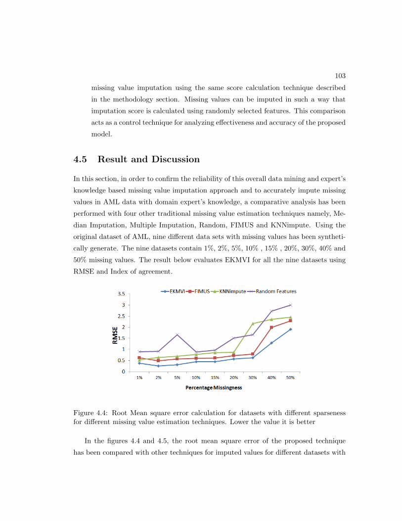
103
missing value imputation using the same score calculation technique described
in the methodology section. Missing values can be imputed in such a way that
imputation score is calculated using randomly selected features. This comparison
acts as a control technique for analyzing effectiveness and accuracy of the proposed
model.
4.5 Result and Discussion
In this section, in order to confirm the reliability of this overall data mining and expert’s
knowledge based missing value imputation approach and to accurately impute missing
values in AML data with domain expert’s knowledge, a comparative analysis has been
performed with four other traditional missing value estimation techniques namely, Me-
dian Imputation, Multiple Imputation, Random, FIMUS and KNNimpute. Using the
original dataset of AML, nine different data sets with missing values has been syntheti-
cally generate. The nine datasets contain 1%, 2%, 5%, 10% , 15% , 20%, 30%, 40% and
50% missing values. The result below evaluates EKMVI for all the nine datasets using
RMSE and Index of agreement.
Figure 4.4: Root Mean square error calculation for datasets with different sparsenessfor different missing value estimation techniques. Lower the value it is better
In the figures 4.4 and 4.5, the root mean square error of the proposed technique
has been compared with other techniques for imputed values for different datasets with

104
Figure 4.5: Root Mean square error calculation for datasets with different sparsenessfor different missing value estimation techniques. Lower the value it is better
different sparseness. It can be seen that in figure 4.4 the proposed technique EKMVI has
less root mean square error (RMSE) than FIMUS [90] and KnnImpute [89] The RMSE
increases with increase in sparseness, specially with knnImpute where error increases
rate is significantly high with increase in missing values. FIMUS has consistently more
error than EKMVI with different levels of sparseness. The increase rate of error for
EKMVI is very low. In figure 4.5 it can be seen that with imputation techniques like
Median imputation and multiple imputation, rate increase rate is significantly higher
than EKMVI with increase in sparseness in the data set (from 1% to 50% sparseness).
With Median imputation technique there is a huge increase in root mean square error.
This is because Median imputation strategy can severely distort the discrete distribution
for this variable, leading to complications with summary measures including, notably,
underestimates of the standard deviation.
In the figures 4.6 and 4.7, EKMVI has been compared with other techniques for
imputed values for different datasets with different sparseness using a measure called
Index of Agreement. The index of agreement tests the degree of resemblance between
actual and imputed values. This value can vary between 0 and 1. The higher is the score ,
the better. It can be observed that in figure 4.6 EKMVI has greater and consistent index
of Agreement than FIMUS [90] and KnnImpute [89]. KnnImpute has consistently low
Index of agreement than the other two method when sparseness increases in the data set.

105
Figure 4.6: Index of Agreement calculation for datasets with different sparseness fordifferent missing value estimation techniques. Higher the value it is better
It is clear that index of agreement decreases with increase in sparseness, specially with
FIMUS where the drop in Index of Agreement score is significantly high with increase
in missing values. KnnImpute has consistently more error than EKMVI with different
percentages of sparseness. The increase in rate of error for EKMVI is very low. Figure
4.7 shows, with imputation techniques like Median imputation, index of agreement is
significantly and consistently lower than EKMVI with increase in sparseness in the data
set (from 1% to 50% sparseness). This is because of the same reason that has been
stated above. With multiple imputation technique this score is same as EKMVI for
5% sparseness in the dataset. As the sparsity increases from 10% to 50% the index of
agreement score drops significantly as compared to EKMVI.
The above result suggest that the proposed missing value imputation technique
EKMVI has a better performance in the domain of HSCT than existing techniques such
as FIMUS, Median imputation, Multiple Imputation and KnnImpute.
4.6 Conclusion
In this work, an expert’s knowledge based missing value imputation technique has been
developed that integrates domain expert’s knowledge with data information to estimate
missing values that is more accurate and effective for improved predictive modeling.
Different levels of sparseness has been evaluated by simulating missing values in the
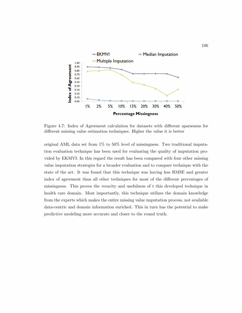
106
Figure 4.7: Index of Agreement calculation for datasets with different sparseness fordifferent missing value estimation techniques. Higher the value it is better
original AML data set from 1% to 50% level of missingness. Two traditional imputa-
tion evaluation technique has been used for evaluating the quality of imputation pro-
vided by EKMVI. In this regard the result has been compared with four other missing
value imputation strategies for a broader evaluation and to compare technique with the
state of the art. It was found that this technique was having less RMSE and greater
index of agreement than all other techniques for most of the different percentages of
missingness. This proves the veracity and usefulness of t this developed technique in
health care domain. Most importantly, this technique utilizes the domain knowledge
from the experts which makes the entire missing value imputation process, not available
data-centric and domain information enriched. This in turn has the potential to make
predictive modeling more accurate and closer to the round truth.

Chapter 5
Conclusion and Discussion
High dimensional and sparse nature of large data sets can pose a significant challenge
in the accuracy of predictive modeling in large health care data sets. Two main goals of
high-dimensional data analysis in the health care domain are to develop effective meth-
ods that can accurately predict the future observations with relevant and non-redundant
features and at the same time to gain insight into the relationship between the features
and response for scientific purposes. Furthermore, due to large sample size, large data
sets give rise to two additional goals: to understand heterogeneity and commonality
across different sub-populations. In other words, in large health care data following
are the expectations: (1) exploring the hidden structures of each sub-population of the
data, which is traditionally not feasible and might even be treated as ’outliers’ when
the sample size is small; (2) extracting significant features across many sub-populations
even when there are large individual variations. 3) Handling data sparseness or the
missing values and estimating values approximately for the missing fields. High dimen-
sional and sparse data causes predictive modeling challenges by bringing information
loss, noise accumulation, spurious correlations and incidental homogeneity which causes
heavy computational cost, algorithmic instability, experimental variations and statisti-
cal bias during data modeling. The field of statistics and data mining on the other hand
accumulated a huge body of literature on various issues of data analysis such as dimen-
sionality reduction, data segmentation and missing value imputation. However, many
of the available insights and techniques have remained limited in application areas such
107
108
as risk analysis and bio-informatics, hence are not readily applicable to the hugely in-
creasing areas of health care. Moreover there is no single system available in the health
care domain that improves predictive model building with the help of different data
segmentation strategies for high dimensionality, heterogeneity and the missing value
imputation problems. This thesis is first of its kind to provide a one stop solution for
large health care data problems by developing and combining different strategies such
as robust feature selection, data segmentation with co-clustering and missing value es-
timation with expert’s knowledge. While doing so, an unique tools has been presented
that is not only robust toward different predictive classification models but also has the
potential to enhance the predictive capabilities in a heterogeneous data set especially
in the health care domain. Further a unique missing value estimation method using
domain expert’s knowledge has been proposed in the health care domain. Finally, it
was observed that, the three unique technique not only these improves predictive per-
formance in health care but also in general is effective as data analysis tools. This has
been proved by evaluating the proposed technique with different publicly available data
sets in this thesis.
In this thesis, it has been illustrated how the challenges of high dimensional and
sparse nature of large data can be approximately overcome beyond general pre-processing
and visualizing of data for significantly improving predictive modeling. In the first part
of the thesis the knowledge of rank aggregation has been utilized to obtain a less biased
and more robust feature selection technique for handling high dimensional data. It was
also empirically illustrated that the proposed approaches are competitive in performance
with the state-of-the-art methods in feature selection. The same has been shown with
the proposed co-clustering technique as well as expert’s knowledge based missing value
imputation technique. The first two techniques have been shown to produce signifi-
cant improvement in predictive modeling in different domain. A separate performance
test was also conducted where each technique developed in this thesis was applied to
the same (AML) data set in various sequence. Random Forest and Logistic Regression
classification algorithm was used for determining the final predictive performance (f-
measure) of the resulting data. The result of this analysis is shown in figure 5.1. The
predictive performance of a learning algorithm in the data without any pre-processing
technique has been compared with different techniques developed in this thesis. The

109
result shows that when different techniques are used in different sequence on the same
data, a significant increase in the predictive power (weighted f-measure) can be observed.
Thus, it is evident that a set of highly useful and efficient pre-processing techniques has
been proposed in this thesis, in the domain of health care for an improved predictive
modeling.
Figure 5.1: Different techniques developed in this thesis in sequence
This study and the developed techniques can be viewed as a first step towards
building a unique system in the health care domain, that handles challenges related
to high dimensional, heterogeneous and sparse health care data for an improved and
more effective predictive model building. Here, some key points has been summarized
to assist future work in this area -
• The proposed work assumes the data sets to be large and not the currently popular
big data. These techniques can be adapted to work in distributed framework
especially the rank aggregation based feature selection technique and predictive
overlapping co-clustering. This would have the potential to be a break through in
the area of predictive analytics in big data paradigm.
• In the expert’s knowledge based missing value imputation, it was assumed that
the variables are categorical. However, this method can be easily extended for
numerical variables as well in the healthcare domain. However, this will require
110
a numerical variable to categorical variable conversion strategy, that converts nu-
merical variables to categorical variables with minimum loss or introducing mini-
mum bias.
• In order to include multiple expert’s opinion strategies such as inter-rater’s agree-
ment can be used for integrating knowledge from multiple source for missing value
imputation as well as other data analysis tasks.
References
[1] R. Tibshirani. Regression shrinkage and selection via the lasso. Journal of the
Royal Statistical Society. Series B (Methodological), pages 267–288, 1996.
[2] Andy Liaw and Matthew Wiener. Classification and regression by randomforest.
R news, 2(3):18–22, 2002.
[3] Chandrima Sarkar, Sarah Cooley, and Jaideep Srivastava. Improved feature selec-
tion for hematopoietic cell transplantation outcome prediction using rank aggre-
gation. In Computer Science and Information Systems (FedCSIS), 2012 Federated
Conference on, pages 221–226. IEEE, 2012.
[4] Thomas W Miller. Web and Network Data Science: Modeling Techniques in
Predictive Analytics. FT Press, 2014.
[5] Trevor Hastie, Robert Tibshirani, and Jerome Friedman. Unsupervised learning.
Springer, 2009.
[6] Anthony Christopher Davison and David Victor Hinkley. Bootstrap methods and
their application, volume 1. Cambridge university press, 1997.
[7] Bradley Efron and Robert J Tibshirani. An introduction to the bootstrap. CRC
press, 1994.
[8] Eric P Xing, Michael I Jordan, Richard M Karp, et al. Feature selection for
high-dimensional genomic microarray data. In ICML, volume 1, pages 601–608.
Citeseer, 2001.
111

112
[9] Y. Yang and J.O. Pedersen. A comparative study on feature selection in text cate-
gorization. In MACHINE LEARNING-INTERNATIONAL WORKSHOP THEN
CONFERENCE-, pages 412–420. MORGAN KAUFMANN PUBLISHERS, INC.,
1997.
[10] Kiansing Ng and Huan Liu. Customer retention via data mining. Artificial Intel-
ligence Review, 14(6):569–590, 2000.
[11] Yong Rui, Thomas S Huang, and Shih-Fu Chang. Image retrieval: Current tech-
niques, promising directions, and open issues. Journal of visual communication
and image representation, 10(1):39–62, 1999.
[12] Srivatsava Daruru, Nena M Marin, Matt Walker, and Joydeep Ghosh. Pervasive
parallelism in data mining: dataflow solution to co-clustering large and sparse
netflix data. In Proceedings of the 15th ACM SIGKDD international conference
on Knowledge discovery and data mining, pages 1115–1124. ACM, 2009.
[13] Harleen Kaur and Siri Krishan Wasan. Empirical study on applications of data
mining techniques in healthcare. Journal of Computer Science, 2(2):194–200,
2006.
[14] Richard Ernest Bellman and Stuart E Dreyfus. Applied dynamic programming.
1962.
[15] Kevin Beyer, Jonathan Goldstein, Raghu Ramakrishnan, and Uri Shaft. When
is nearest neighbor meaningful? In Database TheoryICDT99, pages 217–235.
Springer, 1999.
[16] Mahdi Shafiei and Evangelos Milios. Model-based overlapping co-clustering. In
Proceeding of SIAM Conference on Data Mining, 2006.
[17] Gregory Piateski and William Frawley. Knowledge discovery in databases. MIT
press, 1991.
[18] Guangtao Wang and Qinbao Song. Selecting feature subset for high dimensional
data via the propositional foil rules. Pattern Recognition, 2012.

113
[19] M Termenon, Manuel Grana, A Besga, J Echeveste, and A Gonzalez-Pinto. Lattice
independent component analysis feature selection on diffusion weighted imaging
for alzheimer’s disease classification. Neurocomputing, 114:132–141, 2013.
[20] Yvan Saeys, Inaki Inza, and Pedro Larranaga. A review of feature selection tech-
niques in bioinformatics. Bioinformatics, 23(19):2507–2517, 2007.
[21] J.G. Kemeny. Mathematics without numbers. Daedalus, 88(4):577–591, 1959.
[22] Jean C. de Borda. Memoire sur les Elections au Scrutin. Histoire de l’Academie
Royale des Sciences, Paris, 1781.
[23] I. Guyon and A. Elisseeff. An introduction to variable and feature selection. The
Journal of Machine Learning Research, 3:1157–1182, 2003.
[24] Lei Yu and Huan Liu. Feature selection for high-dimensional data: A fast
correlation-based filter solution. In MACHINE LEARNING-INTERNATIONAL
WORKSHOP THEN CONFERENCE-, volume 20, page 856, 2003.
[25] Ricardo Vilalta and Daniel Oblinger. A quantification of distance bias between
evaluation metrics in classification. In ICML, pages 1087–1094. Citeseer, 2000.
[26] Rinat Khoussainov, Andreas Heß, and Nicholas Kushmerick. Ensembles of bi-
ased classifiers. In Proceedings of the 22nd international conference on Machine
learning, pages 425–432. ACM, 2005.
[27] Thomas Abeel, Thibault Helleputte, Yves Van de Peer, Pierre Dupont, and Yvan
Saeys. Robust biomarker identification for cancer diagnosis with ensemble feature
selection methods. Bioinformatics, 26(3):392–398, 2010.
[28] Mateusz Budnik and Bartosz Krawczyk. On optimal settings of classification tree
ensembles for medical decision support. Health informatics journal, 19(1):3–15,
2013.
[29] Micha l Wozniak, Manuel Grana, and Emilio Corchado. A survey of multiple
classifier systems as hybrid systems. Information Fusion, 16:3–17, 2014.

114
[30] Atanu Roy, Zoheb H Borbora, and Jaideep Srivastava. Socialization and trust
formation: A mutual reinforcement? an exploratory analysis in an online virtual
setting. In Advances in Social Networks Analysis and Mining (ASONAM), 2013
IEEE/ACM International Conference on, pages 653–660. IEEE, 2013.
[31] Vincent Conitzer. Computational aspects of preference aggregation. PhD thesis,
IBM, 2006.
[32] C. Dwork, R. Kumar, M. Naor, and D. Sivakumar. Rank aggregation methods
for the web. In Proceedings of the 10th international conference on World Wide
Web, pages 613–622. ACM, 2001.
[33] Karthik Subbian and Prem Melville. Supervised rank aggregation for predicting
influence in networks. arXiv preprint arXiv:1108.4801, 2011.
[34] J.J. Bartko. On various intraclass correlation reliability coefficients. Psychological
bulletin, 83(5):762, 1976.
[35] Scott L Pomeroy, Pablo Tamayo, Michelle Gaasenbeek, Lisa M Sturla, Michael
Angelo, Margaret E McLaughlin, John YH Kim, Liliana C Goumnerova, Peter M
Black, Ching Lau, et al. Prediction of central nervous system embryonal tumour
outcome based on gene expression. Nature, 415(6870):436–442, 2002.
[36] Santhosh P Pathical. Classification in High Dimensional Feature Spaces through
Random Subspace Ensembles. PhD thesis, University of Toledo, 2010.
[37] S Hettich and SD Bay. The uci kdd archive, 1999.
[38] M. Hall, E. Frank, G. Holmes, B. Pfahringer, P. Reutemann, and I.H. Witten. The
weka data mining software: an update. ACM SIGKDD Explorations Newsletter,
11(1):10–18, 2009.
[39] R. Storb and E.D. Thomas. Allogeneic bone-marrow transplantation. Immuno-
logical reviews, 71(1):77–102, 1983.
[40] S. Cooley, E. Trachtenberg, T.L. Bergemann, K. Saeteurn, J. Klein, C.T. Le,
S.G.E. Marsh, L.A. Guethlein, P. Parham, J.S. Miller, et al. Donors with group

115
b kir haplotypes improve relapse-free survival after unrelated hematopoietic cell
transplantation for acute myelogenous leukemia. Blood, 113(3):726–732, 2009.
[41] S. Cooley, D.J. Weisdorf, L.A. Guethlein, J.P. Klein, T. Wang, C.T. Le, S.G.E.
Marsh, D. Geraghty, S. Spellman, M.D. Haagenson, et al. Donor selection for
natural killer cell receptor genes leads to superior survival after unrelated trans-
plantation for acute myelogenous leukemia. Blood, 116(14):2411–2419, 2010.
[42] M.A. Caligiuri. Human natural killer cells. Blood, 112(3):461–469, 2008.
[43] C.A. Biron, K.S. Byron, and J.L. Sullivan. Severe herpesvirus infections in
an adolescent without natural killer cells. New England Journal of Medicine,
320(26):1731–1735, 1989.
[44] H.G. Shilling, N. Young, L.A. Guethlein, N.W. Cheng, C.M. Gardiner, D. Tyan,
and P. Parham. Genetic control of human nk cell repertoire. The Journal of
Immunology, 169(1):239–247, 2002.
[45] G.D. Tourassi, E.D. Frederick, M.K. Markey, and C.E. Floyd Jr. Application of
the mutual information criterion for feature selection in computer-aided diagnosis.
Medical Physics, 28:2394, 2001.
[46] B. Sahiner, H.P. Chan, D. Wei, N. Petrick, M.A. Helvie, D.D. Adler, and M.M.
Goodsitt. Image feature selection by a genetic algorithm: Application to classifi-
cation of mass and normal breast tissue. Medical Physics, 23:1671, 1996.
[47] H. Peng, F. Long, and C. Ding. Feature selection based on mutual information
criteria of max-dependency, max-relevance, and min-redundancy. Pattern Analysis
and Machine Intelligence, IEEE Transactions on, 27(8):1226–1238, 2005.
[48] I. Levner. Feature selection and nearest centroid classification for protein mass
spectrometry. BMC bioinformatics, 6(1):68, 2005.
[49] T. Dietterich. Ensemble methods in machine learning. Multiple classifier systems,
pages 1–15, 2000.
116
[50] Y. Saeys, T. Abeel, and Y. Van de Peer. Robust feature selection using ensem-
ble feature selection techniques. Machine Learning and Knowledge Discovery in
Databases, pages 313–325, 2008.
[51] M. Colonna and J. Samaridis. Cloning of immunoglobulin-superfamily members
associated with hla-c and hla-b recognition by human natural killer cells. Science,
268(5209):405–408, 1995.
[52] M. Uhrberg, N.M. Valiante, B.P. Shum, H.G. Shilling, K. Lienert-Weidenbach,
B. Corliss, D. Tyan, L.L. Lanier, and P. Parham. Human diversity in killer cell
inhibitory receptor genes. Immunity, 7(6):753–763, 1997.
[53] N. Wagtmann, R. Biassoni, C. Cantoni, S. Verdiani, M.S. Malnati, M. Vitale,
C. Bottino, L. Moretta, A. Moretta, and E.O. Long. Molecular clones of the p58
nk cell receptor reveal immunoglobulin-related molecules with diversity in both
the extra-and intracellular domains. Immunity, 2(5):439–449, 1995.
[54] N.M. Valiante, M. Uhrberg, H.G. Shilling, K. Lienert-Weidenbach, K.L. Arnett,
A. D’Andrea, J.H. Phillips, L.L. Lanier, and P. Parham. Functionally and struc-
turally distinct nk cell receptor repertoires in the peripheral blood of two human
donors. Immunity, 7(6):739–751, 1997.
[55] L. Ruggeri, M. Capanni, E. Urbani, K. Perruccio, W.D. Shlomchik, A. Tosti,
S. Posati, D. Rogaia, F. Frassoni, F. Aversa, et al. Effectiveness of donor nat-
ural killer cell alloreactivity in mismatched hematopoietic transplants. Science’s
STKE, 295(5562):2097, 2002.
[56] S. Giebel, F. Locatelli, T. Lamparelli, A. Velardi, S. Davies, G. Frumento, R. Mac-
cario, F. Bonetti, J. Wojnar, M. Martinetti, et al. Survival advantage with kir
ligand incompatibility in hematopoietic stem cell transplantation from unrelated
donors. Blood, 102(3):814–819, 2003.
[57] S.M. Davies, L. Ruggieri, T. DeFor, J.E. Wagner, D.J. Weisdorf, J.S. Miller, A. Ve-
lardi, and B.R. Blazar. Evaluation of kir ligand incompatibility in mismatched
unrelated donor hematopoietic transplants. Blood, 100(10):3825–3827, 2002.

117
[58] R. Fagin, R. Kumar, and D. Sivakumar. Efficient similarity search and classifica-
tion via rank aggregation. In Proceedings of the 2003 ACM SIGMOD international
conference on Management of data, pages 301–312. ACM, 2003.
[59] Budhaditya Saha, Duc-Son Pham, Dinh Phung, and Svetha Venkatesh. Cluster-
ing patient medical records via sparse subspace representation. In Advances in
Knowledge Discovery and Data Mining, pages 123–134. Springer, 2013.
[60] Thomas George and Srujana Merugu. A scalable collaborative filtering framework
based on co-clustering. In Data Mining, Fifth IEEE International Conference on,
pages 4–pp. IEEE, 2005.
[61] Inderjit S Dhillon, Subramanyam Mallela, and Dharmendra S Modha.
Information-theoretic co-clustering. In Proceedings of the ninth ACM SIGKDD
international conference on Knowledge discovery and data mining, pages 89–98.
ACM, 2003.
[62] Yizong Cheng and George M Church. Biclustering of expression data. In Ismb,
volume 8, pages 93–103, 2000.
[63] Hyuk Cho, Inderjit S Dhillon, Yuqiang Guan, and Suvrit Sra. Minimum sum-
squared residue co-clustering of gene expression data. In SDM, volume 3, page 3,
2004.
[64] Thomas Baumann and Alain J Germond. Application of the kohonen network
to short-term load forecasting. In Neural Networks to Power Systems, 1993. AN-
NPS’93., Proceedings of the Second International Forum on Applications of, pages
407–412. IEEE, 1993.
[65] James C Bezdek, Robert Ehrlich, and William Full. Fcm: The fuzzy c means
clustering algorithm. Computers & Geosciences, 10(2):191–203, 1984.
[66] Ruggero G Pensa and Jean-Francois Boulicaut. Constrained co-clustering of gene
expression data. In SDM, pages 25–36, 2008.

118
[67] Inderjit S Dhillon. Co-clustering documents and words using bipartite spectral
graph partitioning. In Proceedings of the seventh ACM SIGKDD international
conference on Knowledge discovery and data mining, pages 269–274. ACM, 2001.
[68] Eirini Giannakidou, Vassiliki Koutsonikola, Athena Vakali, and Yiannis Kompat-
siaris. Co-clustering tags and social data sources. In Web-Age Information Man-
agement, 2008. WAIM’08. The Ninth International Conference on, pages 317–324.
IEEE, 2008.
[69] Daniel Hanisch, Alexander Zien, Ralf Zimmer, and Thomas Lengauer. Co-
clustering of biological networks and gene expression data. Bioinformatics,
18(suppl 1):S145–S154, 2002.
[70] M Hanmandlu, S Susan, VK Madasu, and BC Lovell. Fuzzy co-clustering of
medical images using bacterial foraging. In Image and Vision Computing New
Zealand, 2008. IVCNZ 2008. 23rd International Conference, pages 1–6. IEEE,
2008.
[71] K Schluter and Detlev Drenckhahn. Co-clustering of denatured hemoglobin with
band 3: its role in binding of autoantibodies against band 3 to abnormal and aged
erythrocytes. Proceedings of the National Academy of Sciences, 83(16):6137–6141,
1986.
[72] Hanhuai Shan and Arindam Banerjee. Bayesian co-clustering. In Data Mining,
2008. ICDM’08. Eighth IEEE International Conference on, pages 530–539. IEEE,
2008.
[73] John A Hartigan. Direct clustering of a data matrix. Journal of the american
statistical association, 67(337):123–129, 1972.
[74] Robert Tibshirani, Trevor Hastie, Mike Eisen, Doug Ross, David Botstein, Pat
Brown, et al. Clustering methods for the analysis of dna microarray data. Dept.
Statist., Stanford Univ., Stanford, CA, Tech. Rep, 1999.
[75] Naftali Tishby, Fernando C Pereira, and William Bialek. The information bottle-
neck method. arXiv preprint physics/0004057, 2000.
119
[76] Krishna Kummamuru, Ajay Dhawale, and Raghu Krishnapuram. Fuzzy co-
clustering of documents and keywords. In Fuzzy Systems, 2003. FUZZ’03. The
12th IEEE International Conference on, volume 2, pages 772–777. IEEE, 2003.
[77] Xufei Wang, Lei Tang, Huiji Gao, and Huan Liu. Discovering overlapping groups
in social media. In Data Mining (ICDM), 2010 IEEE 10th International Confer-
ence on, pages 569–578. IEEE, 2010.
[78] Lani F Wu, Timothy R Hughes, Armaity P Davierwala, Mark D Robinson, Roland
Stoughton, and Steven J Altschuler. Large-scale prediction of saccharomyces cere-
visiae gene function using overlapping transcriptional clusters. Nature genetics,
31(3):255–265, 2002.
[79] Xiaoxiao Shi, Wei Fan, and Philip S Yu. Efficient semi-supervised spectral co-
clustering with constraints. In Data Mining (ICDM), 2010 IEEE 10th Interna-
tional Conference on, pages 1043–1048. IEEE, 2010.
[80] Meghana Deodhar and Joydeep Ghosh. A framework for simultaneous co-
clustering and learning from complex data. In Proceedings of the 13th ACM
SIGKDD international conference on Knowledge discovery and data mining, pages
250–259. ACM, 2007.
[81] Scott Kirkpatrick, D. Gelatt Jr., and Mario P Vecchi. Optimization by simmulated
annealing. science, 220(4598):671–680, 1983.
[82] Malika Charrad and Mohamed Ben Ahmed. Simultaneous clustering: A survey.
In Pattern Recognition and Machine Intelligence, pages 370–375. Springer, 2011.
[83] Nikhil R Pal and James C Bezdek. On cluster validity for the fuzzy c-means
model. Fuzzy Systems, IEEE Transactions on, 3(3):370–379, 1995.
[84] the original movielens dataset from grouplens research group.
”http://www.grouplens.org”.
[85] K. Bache and M. Lichman. UCI machine learning repository, 2013.

120
[86] Chandrima Sarkar, Sarah Cooley, and Jaideep Srivastava. Improved feature se-
lection for hematopoietic cell transplantation outcome prediction using rank ag-
gregation.
[87] Chandrima Sarkar, Sarah Cooley, and Jaideep Srivastava. Robust feature selection
technique using rank aggregation. Applied Artificial Intelligence, 28(3):243–257,
2014.
[88] Mohiuddin Ahmed, Abdun Naser Mahmood, and Michael J Maher. Heart disease
diagnosis using co-clustering.
[89] Olga Troyanskaya, Michael Cantor, Gavin Sherlock, Pat Brown, Trevor Hastie,
Robert Tibshirani, David Botstein, and Russ B Altman. Missing value estimation
methods for dna microarrays. Bioinformatics, 17(6):520–525, 2001.
[90] Md Geaur Rahman and Md Zahidul Islam. Fimus: A framework for im-
puting missing values using co-appearance, correlation and similarity analysis.
Knowledge-Based Systems, 56:311–327, 2014.
[91] Orly Alter, Patrick O Brown, and David Botstein. Singular value decomposition
for genome-wide expression data processing and modeling. Proceedings of the
National Academy of Sciences, 97(18):10101–10106, 2000.
[92] Soumya Raychaudhuri, Joshua M Stuart, Russ B Altman, et al. Principal compo-
nents analysis to summarize microarray experiments: application to sporulation
time series. In Pac Symp Biocomput, volume 5, pages 455–466. World Scientific,
2000.
[93] Chandrima Sarkar and Jaideep Srivastava. Impact of density of lab data in ehr
for prediction of potentially preventable events. In Healthcare Informatics (ICHI),
2013 IEEE International Conference on, pages 529–534. IEEE, 2013.
[94] Usama Fayyad, Gregory Piatetsky-Shapiro, and Padhraic Smyth. The kdd process
for extracting useful knowledge from volumes of data. Communications of the
ACM, 39(11):27–34, 1996.
121
[95] Prasanna Desikan, Nisheeth Srivastava, Tamara Winden, Tammie Lindquist,
Heather Britt, and Jaideep Srivastava. Early prediction of potentially preventable
events in ambulatory care sensitive admissions from clinical data. In Healthcare
Informatics, Imaging and Systems Biology (HISB), 2012 IEEE Second Interna-
tional Conference on, pages 124–124. IEEE, 2012.
[96] Ash A Alizadeh, Michael B Eisen, R Eric Davis, Chi Ma, Izidore S Lossos, An-
dreas Rosenwald, Jennifer C Boldrick, Hajeer Sabet, Truc Tran, Xin Yu, et al.
Distinct types of diffuse large b-cell lymphoma identified by gene expression pro-
filing. Nature, 403(6769):503–511, 2000.
[97] Andrew Gelman and Jennifer Hill. Data analysis using regression and multi-
level/hierarchical models. Cambridge University Press, 2006.
[98] Jacob Anhøj. Generic design of web-based clinical databases. Journal of Medical
Internet Research, 5(4), 2003.
[99] Torben Bach Pedersen and Christian S Jensen. Research issues in clinical data
warehousing. In Scientific and Statistical Database Management, 1998. Proceed-
ings. Tenth International Conference on, pages 43–52. IEEE, 1998.
[100] Thomas J Eggebraaten, Jeffrey W Tenner, and Joel C Dubbels. A health-care
data model based on the hl7 reference information model. IBM Systems Journal,
46(1):5–18, 2007.
[101] Shoaib Sehgal, Iqbal Gondal, and Laurence Dooley. A collimator neural network
model for the classification of genetic data. 2004.
[102] Trond Hellem Bø, Bjarte Dysvik, and Inge Jonassen. Lsimpute: accurate esti-
mation of missing values in microarray data with least squares methods. Nucleic
acids research, 32(3):e34–e34, 2004.
[103] Muhammad Shoaib B Sehga, Iqbal Gondal, and Laurence Dooley. Statistical neu-
ral networks and support vector machine for the classification of genetic mutations
in ovarian cancer. In Computational Intelligence in Bioinformatics and Compu-
tational Biology, 2004. CIBCB’04. Proceedings of the 2004 IEEE Symposium on,
pages 140–146. IEEE, 2004.

122
[104] Hsiuying Wang, Chia-Chun Chiu, Yi-Ching Wu, and Wei-Sheng Wu. Shrinkage
regression-based methods for microarray missing value imputation. BMC systems
biology, 7(Suppl 6):S11, 2013.
[105] Estevam R Hruschka Jr, Eduardo R Hruschka, and Nelson FF Ebecken. Bayesian
networks for imputation in classification problems. Journal of Intelligent Infor-
mation Systems, 29(3):231–252, 2007.
[106] Geaur Rahman and Zahidul Islam. A decision tree-based missing value imputation
technique for data pre-processing. In Proceedings of the Ninth Australasian Data
Mining Conference-Volume 121, pages 41–50. Australian Computer Society, Inc.,
2011.
[107] Chengqi Zhang, Yongsong Qin, Xiaofeng Zhu, Jilian Zhang, and Shichao Zhang.
Clustering-based missing value imputation for data preprocessing. In Industrial
Informatics, 2006 IEEE International Conference on, pages 1081–1086. IEEE,
2006.
[108] Alan Wee-Chung Liew, Ngai-Fong Law, and Hong Yan. Missing value imputation
for gene expression data: computational techniques to recover missing data from
available information. Briefings in bioinformatics, 12(5):498–513, 2011.
[109] Hyunsoo Kim, Gene H Golub, and Haesun Park. Missing value estimation for dna
microarray gene expression data: local least squares imputation. Bioinformatics,
21(2):187–198, 2005.
[110] Ki-Yeol Kim, Byoung-Jin Kim, and Gwan-Su Yi. Reuse of imputed data in mi-
croarray analysis increases imputation efficiency. BMC bioinformatics, 5(1):160,
2004.
[111] Lıgia P Bras and Jose C Menezes. Improving cluster-based missing value estima-
tion of dna microarray data. Biomolecular engineering, 24(2):273–282, 2007.
[112] Rebecka Jornsten, Hui-Yu Wang, William J Welsh, and Ming Ouyang. Dna
microarray data imputation and significance analysis of differential expression.
Bioinformatics, 21(22):4155–4161, 2005.

123
[113] Xiangchao Gan, Alan Wee-Chung Liew, and Hong Yan. Microarray missing data
imputation based on a set theoretic framework and biological knowledge. Nucleic
Acids Research, 34(5):1608–1619, 2006.
[114] Johannes Tuikkala, Laura Elo, Olli S Nevalainen, and Tero Aittokallio. Improving
missing value estimation in microarray data with gene ontology. Bioinformatics,
22(5):566–572, 2006.
[115] Qian Xiang, Xianhua Dai, Yangyang Deng, Caisheng He, Jiang Wang, Jihua Feng,
and Zhiming Dai. Missing value imputation for microarray gene expression data
using histone acetylation information. BMC bioinformatics, 9(1):252, 2008.
[116] Peter Johansson and Jari Hakkinen. Improving missing value imputation of mi-
croarray data by using spot quality weights. BMC bioinformatics, 7(1):306, 2006.
[117] Rebecka Jornsten, Ming Ouyang, and Hui-Yu Wang. A meta-data based method
for dna microarray imputation. BMC bioinformatics, 8(1):109, 2007.
[118] Valerie Crooks, Susan Waller, Tom Smith, and Theodore J Hahn. The use of
the karnofsky performance scale in determining outcomes and risk in geriatric
outpatients. Journal of gerontology, 46(4):M139–M144, 1991.
[119] Jochen Hipp, Ulrich Guntzer, and Gholamreza Nakhaeizadeh. Algorithms for
association rule mininga general survey and comparison. ACM sigkdd explorations
newsletter, 2(1):58–64, 2000.
[120] Rakesh Agrawal, Tomasz Imielinski, and Arun Swami. Mining association rules
between sets of items in large databases. In ACM SIGMOD Record, volume 22,
pages 207–216. ACM, 1993.
[121] Helen Giggins and Ljiljana Brankovic. Vicus: a noise addition technique for cat-
egorical data. In Proceedings of the Tenth Australasian Data Mining Conference-
Volume 134, pages 139–148. Australian Computer Society, Inc., 2012.
[122] Eric J Krieg. Statistics and Data Analysis for Social Science. Allyn & Bacon,
2012.
124
[123] Cort J Willmott. Some comments on the evaluation of model performance. Bul-
letin of the American Meteorological Society, 63(11):1309–1313, 1982.
[124] Heikki Junninen, Harri Niska, Kari Tuppurainen, Juhani Ruuskanen, and Mikko
Kolehmainen. Methods for imputation of missing values in air quality data sets.
Atmospheric Environment, 38(18):2895–2907, 2004.
[125] James Honaker and Gary King. What to do about missing values in time-series
cross-section data. American Journal of Political Science, 54(2):561–581, 2010.