Embed Size (px)
Citation preview

IMPROVING RELIABILITY AND ASSESSING
PERFORMANCE OF GLOBAL NAVIGATION
SATELLITE SYSTEM PRECISE POINT
POSITIONING AMBIGUITY RESOLUTION
GARRETT SEEPERSAD
A DISSERTATION SUBMITTED TO THE FACULTY OF GRADUATE STUDIES
IN PARTIAL FULFILLMENT OF THE REQUIREMENTS FOR THE DEGREE OF
DOCTOR OF PHILOSOPHY
GRADUATE PROGRAMME IN EARTH AND SPACE SCIENCE
YORK UNIVERSITY
TORONTO, ONTARIO
AUGUST, 2018
© GARRETT SEEPERSAD, 2018

ii
ABSTRACT
Conventional Precise Point Positioning (PPP) has always required a relatively long
initialization period (few tens of minutes at least) for the carrier-phase ambiguities to
converge to constant values and for the solution to reach its optimal precision. The classical
PPP convergence period is primarily caused by the estimation of the carrier-phase
ambiguity from the relatively noisy pseudoranges and the estimation of atmospheric delay.
If the underlying integer nature of the ambiguity is known, it can be resolved, thereby
reducing the convergence time of conventional PPP.
To recover the underlying integer nature of the carrier-phase ambiguities, different
strategies for mitigating the satellite and receiver dependent equipment delays have been
developed, and products made publicly available to enable ambiguity resolution without
any baseline restrictions. There has been limited research within the scope of
interoperability of the products, combining the products to improve reliability and
assessment of ambiguity resolution within the scope of being an integrity indicator. This
study seeks to develop strategies to enable each of these and examine their feasibility.
The advantage of interoperability of the different PPP ambiguity resolution (PPP-AR)
products would be to permit the PPP user to transform independently generated PPP-AR
products to obtain multiple fixed solutions of comparable precision and accuracy. The
ability to provide multiple solutions would increase the reliability of the solution for, e.g.,
real-time processing: if there were an outage in the generation of the PPP-AR products, the
user could instantly switch streams to a different provider.

iii
The satellite clock combinations routinely produced within the International GNSS Service
(IGS) currently disregard that analysis centers (ACs) provide products which enable
ambiguity resolution. Users have been expected to choose either an IGS product which is
a combined product from multiple ACs or select an individual AC solution which provides
products that enable PPP-AR. The goal of the novel research presented was to develop and
test a robust satellite clock combination preserving the integer nature of the carrier-phase
ambiguities at the user end. mm-level differences were noted, which was expected as the
strength lies mainly in its reliability and stable median performance and the combined
product is better than or equivalent to any single AC’s product in the combination process.
As have been shown in relative positioning and PPP-AR, ambiguity resolution is critical
for enabling cm-level positioning. However, what if specifications where at the few dm-
level, such as 10 cm and 20 cm horizontal – what role does ambiguity resolution play? The
role of ambiguity resolution relies primarily on what are the user specifications. If the user
specifications are at the few cm-level, ambiguity resolution is an asset as it improves
convergence and solution stability. Whereas, if the user’s specification is at the few dm-
level, ambiguity resolution offers limited improvement over the float solution. If the user
has the resources to perform ambiguity resolution, even when the specifications are at the
few dm-level, it should be utilized.

iv
DEDICATION
To: Grandma, Mom, Dad, Dawn, Noah, Glenroy and Alexandra

v
ACKNOWLEDGEMENTS
As with most journeys in life, this thesis took me along a pathway that I could have never
predicted. It could not have been completed successfully without the invaluable support
from several people.
Especial thanks to my supervisor, Dr. Sunil Bisnath who provided me with the opportunity
to embark on this journey. He never ceased to challenge me, redirected my path after each
setback, and always encouraged me to believe in myself as I forged ahead. He also created
countless networking opportunities for me through conferences and multiple internships
for which I am extremely grateful. Thanks to Dr. Bisnath for his invaluable support with
technical advice, financial assistance, and an amicable work environment. I also wish to
thank Drs. Jian-Guo Wang, Spiros Pagiatakis and Costas Armenakis for their priceless
corridor consultations and insightful feedback.
A memorable guest lecture from the late Dr. Kees de Jong in 2013 at York University,
Canada led to an internship at Fugro Intersite, Netherlands. The work relationship with
Drs. Kees de Jong, Xianglin Liu and Matthew Goode and Ms. Karin Cambier at Fugro was
commendable. The experience obtained from this internship augured well with core of my
research. Special thanks to the Etienne van der Kuij of ProTanks Group in Rotterdam,
Netherlands for the first-hand knowledge gained in assessing the performance of GNSS
within the Rotterdam World Gateway (RWG).
In 2016, I was selected to serve at the Geodetic Surveying Division of the Canadian Federal
Government as part of the Research Affiliate Program (RAP). I am deeply indebted to Dr.

vi
Simon Banville, Paul Collins and François Lahaye for their shrewd and skillful
supervision. To the pioneers of Precise Point Positioning, Jan Kouba and Pierre Héroux,
my direct consultation with them is invaluable. A special thanks to Paul for his innovative
techniques in the development of the decoupled clock model which serves as the
foundation of this research. I also wish to acknowledge NRCan for providing the base PPP
code and PPP expertise.
York University was not just a school, but also a home and my colleagues and I became a
family. A special thanks to John Aggrey, Amir Saeidi, Amandeep Mander, Surabhi
Guruprasad, Maninder Gill and Siddharth Dave. Thanks to John for his contributions to
the development of the YorkU-PPP software. Without his support, YorkU-PPP could not
have been the powerful tool that it is today.
While the journey of a PhD takes a lot of self discipline, dedication and hard work none of
it would have been possible without the support of my family. Thanks to Grandma, Mom,
Dad, Dawn, Noah, Glenroy, Shiva, Alexandra, Taylia, Shana, Ravi, Damian, Vivek and
Vachan. I will always be indebted to them for their prayers, sacrifices and encouragements.
vii
TABLE OF CONTENTS
Abstract ............................................................................................................................... ii
Dedication .......................................................................................................................... iv
Acknowledgements ............................................................................................................. v
Table of Contents .............................................................................................................. vii
List of Tables ..................................................................................................................... xi
List of Figures ................................................................................................................... xii
List of Acronyms ............................................................................................................ xvii
List of Symbols ................................................................................................................ xxi
CHAPTER 1 Introduction into PPP GNSS measurement processing ................................... 1
The origins of Precise Point Positioning ............................................................. 2
Review of PPP ambiguity resolution .................................................................. 9
GNSS performance parameters ......................................................................... 13
Problem Statement ............................................................................................ 17
Thesis Statement ............................................................................................... 19
Research Contributions ..................................................................................... 19
Thesis Outline ................................................................................................... 22
CHAPTER 2 Evolution of the PPP user model ................................................................... 25
Introduction into Point Positioning ................................................................... 25
Conventional PPP model .................................................................................. 26
PPP-AR model .................................................................................................. 30

viii
2.3.1 Receiver equipment delay ............................................................................. 36
2.3.2 Satellite equipment delay .............................................................................. 39
Slant ionosphere estimation .............................................................................. 39
Multi-GNSS PPP .............................................................................................. 46
Multi-frequency PPP ......................................................................................... 51
Summary of PPP evolution ............................................................................... 54
CHAPTER 3 Examination of the interoperability PPP-AR products .................................. 57
Introduction into PPP-AR product interoperability .......................................... 57
PPP-AR Products .............................................................................................. 60
3.2.1 Decoupled clocks .......................................................................................... 60
3.2.2 Fractional Cycle Bias .................................................................................... 65
3.2.3 Integer Recovery Clock ................................................................................ 69
3.2.4 Summary of available PPP-AR products ...................................................... 73
Dataset and processing parameters used to quantify performance of PPP-AR 76
Performance of transformed products ............................................................... 78
Challenges in interoperability of PPP-AR products ......................................... 83
3.5.1 Axis convention ............................................................................................ 83
3.5.2 Yaw manoeuvres during satellite eclipse ...................................................... 84
Summary of the performance of PPP-AR product interoperability .................. 86
CHAPTER 4 Improving reliability of PPP-AR products ..................................................... 89
Introduction to satellite clock combination ....................................................... 89
Satellite clock combination of common clocks ................................................ 91
Combining clock products that enable PPP-AR ............................................... 94

ix
4.3.1 Combination process of PPP-AR clock products ......................................... 95
4.3.2 Combined clock products ............................................................................. 96
Aligning IGS common clocks to clock products that enable PPP-AR ........... 102
Performance of combined satellite clock products ......................................... 104
Summary of the benefits of combining AR products ..................................... 107
CHAPTER 5 Reassessing the role of ambiguity resolution in PPP ................................... 110
Introduction ..................................................................................................... 110
Ambiguity resolution ...................................................................................... 112
5.2.1 Partial Ambiguity resolution ....................................................................... 112
5.2.2 Resolving and fixing the ambiguities ......................................................... 114
Ambiguity validation ...................................................................................... 117
Assessment of the role of ambiguity resolution in PPP .................................. 119
5.4.1 Convergence ............................................................................................... 120
5.4.2 Position uncertainty .................................................................................... 125
5.4.3 Post-fit and integer-fit residuals .................................................................. 128
Conclusions ..................................................................................................... 134
CHAPTER 6 Conclusions and Recommendations for Future Research ............................ 137
Research Conclusions ..................................................................................... 137
6.1.1 Uncombining the PPP representation ......................................................... 138
6.1.2 Interoperability of the PPP-AR products .................................................... 139
6.1.3 Combining the PPP-AR products ............................................................... 141
6.1.4 Re-examining the role of ambiguity resolution .......................................... 143
Research recommendations for the near future .............................................. 143
x
6.2.1 Real time PPP-AR with low GNSS receiver and antenna .......................... 144
6.2.2 Improving the stochastic model .................................................................. 145
6.2.3 Low-cost, multi-sensor integration ............................................................. 146
6.2.4 A priori atmospheric corrections ................................................................ 148
References ....................................................................................................................... 150
xi
LIST OF TABLES
Table 1.1 Summary of error sources in PPP, mitigative strategy and residuals (Seepersad
and Bisnath 2014a) ............................................................................................................. 6
Table 2.1: Preferred measurements within YorkU-PPP multi-GNSS model. .................. 56
Table 3.1: Comparison of different public providers of products to enable PPP-AR ...... 75
Table 3.2: Summary of the transformation of the PPP-AR products to the combined DCM
format and uncombined representation ............................................................................. 76
Table 3.3: rms error of the final solution produced by YorkU-PPP from 24-hour datasets
using data from 155 sites for DOY 178 to 184, GPS week 1903, of 2016 provided by the
IGS. Satellite products were provided by NRCan, CNES and Wuhan University. All units
are in millimetres. ............................................................................................................. 79
Table 4.1: Estimated parameters in satellite clock combination and associated constraints.
........................................................................................................................................... 93
Table 4.2: Fixed terms in the adjustment to remove rank deficiency. .............................. 94
Table 5.1: Summary statistics of ambiguity resolved, and ambiguity validated solutions
for the station ALGO. Statistics compares the performance of ambiguity validation in
relative positioning and PPP-AR. GNSS data from DOY 178 of 2016 was used. All units
are in cm. ......................................................................................................................... 134
xii
LIST OF FIGURES
Figure 1.1 Fundamental idea underlying the SPS technique as compared to PPP
(Seepersad and Bisnath 2014a). .......................................................................................... 4
Figure 1.2 Range to position and time domain transformations in PPP data processing
illustrating the different domains of PPP error sources (Seepersad and Bisnath 2014a). ... 5
Figure 1.3: Current research areas in Precise Point Positioning. ........................................ 8
Figure 1.4: Illustration of the difference between the “float” and “fixed” solution in the
horizontal component. NRC1 DOY 179, 2016 located in Ottawa, Canada. .................... 10
Figure 1.5: Evolution of the PPP user model. ................................................................... 11
Figure 1.6 Current research areas within PPP ambiguity resolution. ............................... 13
Figure 1.7 Multi-GNSS Experiment (MGEX) product availability (IGS 2018a) ............ 15
Figure 2.1: Conceptual illustration of the integer nature of the ambiguity term affected by
receiver and satellite equipment delays. ........................................................................... 29
Figure 2.2: Different correction terms transmitted in observation space and state space
representation (Wübbena 2012). ....................................................................................... 33
Figure 2.3: Illustration of the residuals for PRN 4 of P1 and P2 pseudorange
measurements, combined P1 and P2 and linearly combined ionosphere-free pseudorange
measurements for the site NRC1 DOY 178 of 2016 located in Ottawa, Canada. ............ 46
Figure 2.4: Transition towards the uncombined PPP mathematical model. ..................... 56
Figure 3.1: Relative satellite carrier-phase clock correction provided by NRCan on DOY
178 of 2016 for PRN 28 (relative to PRN 5). Linear trend has been removed. All units are
in metres. ........................................................................................................................... 62
Figure 3.2: Satellite code clock offset provided by NRCan on DOY 178 of 2016 for PRN
28. All units are in metres. ................................................................................................ 62

xiii
Figure 3.3: Satellite widelane correction provided by NRCan on DOY 178 of 2016 for
PRN 28. All units are in metres. ....................................................................................... 63
Figure 3.4: Code dependent equipment delay corrections. Corrections were generated
from products provided by NRCan on DOY 178 of 2016 for PRN 28. All units are in
metres. ............................................................................................................................... 65
Figure 3.5: Relative satellite carrier-phase clock correction provided by Wuhan
University utilizing IGS products on DOY 178 of 2016 for PRN 28 (relative to PRN 5).
Linear trend has been removed. All units are in metres. .................................................. 66
Figure 3.6: L1 satellite equipment delay provided by Wuhan University on DOY 178 of
2016 for PRN 28. All units are in metres.......................................................................... 67
Figure 3.7: Wide lane satellite equipment delay provided by Wuhan University on DOY
178 of 2016 for PRN 28. All units are in metres. ............................................................. 67
Figure 3.8: Uncombined code satellite equipment delay provided by Wuhan University
on DOY 178 of 2016 for PRN 28 using IGS Final products. All units are in metres. ..... 69
Figure 3.9: Relative satellite carrier-phase clock correction provided by CNES on DOY
178 of 2016 for PRN 28 (relative to PRN 5). Linear trend has been removed. All units are
in metres. ........................................................................................................................... 71
Figure 3.10: Wide lane correction provided by CNES on DOY 178 of 2016 for PRN 28.
All units are in metres. ...................................................................................................... 71
Figure 3.11: Uncombined satellite code clock provided by CNES on DOY 178 of 2016
for PRN 28. All units are in metres................................................................................... 73
Figure 3.12: Uncombined satellite phase clock provided by CNES on DOY 178 of 2016
for PRN 28. All units are in metres................................................................................... 73
Figure 3.13: Global distribution of the selected 155 IGS stations observed during DOY
178 to 184, GPS week 1903, of 2016. .............................................................................. 78

xiv
Figure 3.14: Site NRC1 DOY 178 of 2016 located in Ottawa, Canada, illustrating the
differences between the “float” and “fixed” solution in the horizontal component where
insets for each figure represents the initial 30 minutes of convergence time. Limits of y-
axis represents position error. ........................................................................................... 81
Figure 3.15: Site NRC1 DOY 178 of 2016 located in Ottawa, Canada, illustrating the
differences between the “float” and “fixed” solution in the vertical component where
insets for each figure represents the initial 30 minutes of convergence time. Limits of y-
axis represents position error. ........................................................................................... 82
Figure 3.16: Orientation of the spacecraft body frame for GPS Block IIR/IIR-M satellites
(a) manufacturer specification system; (b) IGS axis conventions (Montenbruck et al.
2015). ................................................................................................................................ 84
Figure 3.17: Geometry of an eclipsing satellite, where is elevation of the Sun above the
orbital plane and is the spacecraft’s geocentric orbit angle. “Midnight” denotes the
farthest point of the orbit from the Sun whereas “noon” denotes the closest point. From
Dilssner et al. (2011). ........................................................................................................ 86
Figure 4.1: Overview of the steps required to combine satellite clocks products that
enable PPP-AR.................................................................................................................. 95
Figure 4.2: Inconsistent error modelling during a satellite eclipse for PRN 24 with respect
to PRN 1, Block IIF on DOY 178 of 2016 between IRC and DCM. ............................... 98
Figure 4.3: Convergence of the forward run of DCM L1 satellite offset with respect to the
IRC on DOY 178, 2016 with the differences in yaw manoeuvres and axis convention
taken into consideration. Each colour represents a different satellite with the integer
component removed from each time series. ..................................................................... 99
Figure 4.4: Convergence of the DCM L1 satellite offsets with respect to the IRC for DOY
179, 2016 with the differences in axis convention not account for. Each colour represents
a different satellite with the integer component removed from each time series. ............ 99

xv
Figure 4.5: Convergence of the DCM L1 satellite offset with respect to the IRC on DOY
179, 2016 with the differences in axis convention account for. Each colour represents a
different satellite with the integer component removed from each time series. ............. 100
Figure 4.6: Convergence of the DCM widelane satellite offset with respect to the IRC on
DOY 178, 2016. Each colour represents a different satellite with the integer component
removed from each time series. ...................................................................................... 101
Figure 4.7: Time reference parameter of DCM with respect to IRC on DOY 178, 2016.
......................................................................................................................................... 101
Figure 4.8: Post-fit residuals of the combined clock (IRC and DCM) with respect to the
reference clock (IRC) on DOY 178, 2016. ..................................................................... 102
Figure 4.9: Convergence of the forward run of IGS L1 satellite offset with respect to the
IRC on DOY 178, 2016. Each colour represents a different satellite with an integer
component removed from each time series. ................................................................... 103
Figure 4.10: Time reference parameter of IGS with respect to IRC on DOY 178, 2016.
......................................................................................................................................... 103
Figure 4.11: Post-fit residuals of the combined clock (IRC and IGS) with respect to the
reference clock (IRC) on DOY 178, 2016. ..................................................................... 104
Figure 4.12: Overview of analysis centres used to generate combined products IGS-AR
and IRC+DCM ................................................................................................................ 105
Figure 4.13: Examination of the repeatability of the PPP user solution in static mode
utilizing different types of clock products. Statistics are based on GPS data from 155 IGS
stations were observed during DOY 178 to 184, of 2016. All units are in millimetres. 106
Figure 4.14: Examination of the repeatability of the PPP user solution in kinematic mode
utilizing different types of clock products. Statistics are based on GPS data from 155 IGS
stations were observed during DOY 178 to 184, of 2016. All units are in millimetres. 107
Figure 5.1: Schematic approach to fixing (Collins et al. 2010). ..................................... 117

xvi
Figure 5.2: Definition of convergence. ........................................................................... 122
Figure 5.3: Cumulative histogram illustrating the required convergence of time to attain
20 cm horizontal for the float and fixed solutions. ......................................................... 123
Figure 5.4: Cumulative histogram illustrating the required convergence of time attain 10
cm horizontal for the float and fixed solutions. .............................................................. 124
Figure 5.5 Cumulative histogram illustrating the required convergence of time attain 2.5
cm horizontal for the float and fixed solutions. .............................................................. 125
Figure 5.6: Solution integrity for the horizontal component. ......................................... 128
Figure 5.7: Performance of ambiguity validated solution at site ALGO DOY 178 of 2016
located in Algonquin Park, Canada. Upper plot illustrates the easting component and the
lower plot is the northing component. ............................................................................ 130
Figure 5.8: Station distribution used to compare the performance of ambiguity validation
in single baseline relative positioning and PPP-AR. ...................................................... 131
Figure 5.9: Comparison of the ambiguity validated solution between long single baseline
relative positioning and PPP-AR. For relative positioning ALGO was coordinated with
respect to BAIE with a baseline length of 819 km and with respect to NRC1 199 km.
GNSS data from DOY 178 of 2016 was used. ............................................................... 133

xvii
LIST OF ACRONYMS
AC Analysis Centre
AR Ambiguity resolution
BeiDou/BDS Chinese Navigation Satellite System
CC1 Common Clock model
CDDIS Crustal Dynamics Data Information System
CDMA Code Division Multiple Access
CIR Cascade Integer Resolution
CNES Centre National d'Etudes Spatiales
CODE Center for Orbit Determination in Europe
DCB Differential Code Bias
DCM Decoupled Clock Model
DGPS Differential GPS
DOY Day of year
EWL Extra widelane
FARA Fast Ambiguity Resolution Approach
FASF Fast Ambiguity Search Filter
FCB Fractional Cycle Biases
FDMA Frequency Division Multiple Access
GALILEO European Navigation Satellite System
GBAS Ground-Based Augmentation System
GEO Geostationary Orbit
GF Geometry Free

xviii
GFZ GeoForschungsZentrum, Germany
GLONASS Russian Navigation Satellite System
GNSS Global Navigation Satellite System
GPS United States Navigation Satellite System
GRG CNES IGS analysis center solution
GRGS Le Groupe de Recherche de Géodésie Spatiale
ICB Inter-frequency Channel Bias
IF Ionosphere-free linear combination
IGN Institut Geographique National, France
IGR IGS Rapid
IGS International GNSS Service
IRC Integer Recovery Clock
JPL Jet Propulsion Lab
KASI Korean Astronomy and Space Science Institute
LAMBDA Least-squares AMBiguity Decorrelation Adjustment
LSAST Least-Squares Ambiguity Search Technique
MEO Medium Earth Orbit
MGEX Multi-GNSS Experiment
MLAMBDA Modified LAMBDA
MW Melbourne-Wübbena
NAS National Airspace System
NL Narrowlane linear combination
NNSS U.S. Navy Navigation Satellite System

xix
NRCan Natural Resources Canada
NRTK Network RTK
OMEGA Optimal Method for Estimating GPS Ambiguities
OSR Observation Space Representation
PPP Precise Point Positioning
PPP-AR Precise Point Positioning Ambiguity Resolved
PPS Precise Positioning Service
PRN Pseudorandom noise
PTC Positive Train Control
QC Quality Control
RAP Research Affiliate Program (RAP) of the Canadian Federal
Government
RINEX Receiver Independent Exchange Format
RTCM Radio Technical Commission for Maritime Services
RTK Real Time Kinematic
RTKLIB Real Time Kinematic Library
SAVO Sequential fixing Ascending Variance Order
SBAS Satellite-Based Augmentation Systems
SEBLO Sequential BLewitt fixing Order
SGG-WHU Wuhan University School of Geodesy and Geomatics
SINEX Site Independent Exchange Format
SOFOS Sequential Optimum Fixing Order Search
SPP Single Point Positioning
SPS Standard Positioning Service

xx
SSR State Space Representation
TCAR Three Carrier Ambiguity Resolution
TEC Total Electron Content
TTFF Time to first fix
UPD Uncalibrated Phase Delay
VTEC Vertical Total Electron Content
WAAS Wide Area Augmentation System
WL Widelane linear combination
YorkU York University
YorkU-PPP PPP software developed at York University

xxi
LIST OF SYMBOLS
i identifies frequency-dependant terms
P measured pseudorange on iL (m)
measured carrier-phase on iL (m)
dt clock error (m) common to pseudorange and carrier-phase
measurements
t clock error (m) common to carrier-phase measurements only
true geometric range (m)
d code equipment delay (m)
carrier-phase equipment delay (m)
measurement combination co-efficient
measurement combination co-efficient
wavelength (m)
A carrier-phase ambiguity (m)
N carrier-phase ambiguity (cycles)
I slant ionosphere delay on iL (m)
i constant 2
1
2
i
f
f= frequency dependent coefficient
u user position
FCBa measurement equipment delay generated using FCB model
s satellites
m number of visible satellites from user’s position
dt combined clock error
aB AC-specific bias
a analysis centre
n number of analysis centres
s
a consistency correction

xxii
s
aX AC satellite position vector
s
IGSX the IGS combined satellite position vector
aD geocentre offset vector provided by the respective AC
computation of the radius vector with respect to the centre of the Earth
combined equipment delay
K Boolean matrix
c vacuum speed of light (m/s)
pre-selected ratio threshold

1
CHAPTER 1 INTRODUCTION INTO PPP GNSS
MEASUREMENT PROCESSING
Navigation is a very ancient skill or art, which has become a complex science. It is
essentially about travel and finding the way from one place to another and there are a
variety of means by which this objective may be achieved (Britting 1971). Navigation has
been evolving since the beginning of human history and has always been a critical aspect
in our (society’s) development. Navigation systems have taken many forms, varying from
simple ones such as those making use of landmarks, compasses and stars, to more modern
techniques such as the utilization of artificial satellites.
Satellite-based navigation technology was introduced in the early 1960s. The first such
system was the U.S. Navy Navigation Satellite System (NNSS), known as TRANSIT, in
which the receiver measured Doppler shifts of the signal as the satellite transited with a
navigational accuracy of 25-500 m. In 1978, the Global Positioning System (GPS) was
introduced. GPS is a satellite-based radio-positioning and time transfer system designed to
provide all-weather, 24-hour coverage for military users and reduced accuracy for civilian
users. Since then, it has become the backbone of a whole body of navigation and
positioning technologies.
Currently, the U.S., Russia, the European Union (E.U.), and China are each operating or in
the case of the latter two, developing individual Global Navigation Satellite Systems
(GNSS’s): GPS, GLONASS, GALILEO and BeiDou, respectively. Evolving GNSSs can
provide the worldwide community with several benefits, such as the ability to work in

2
challenging environments with limited visibility of satellites, increased positioning
accuracy, more robust detection and exclusion of anomalies, more accurate timing
reference as well as improved estimation of tropospheric and ionospheric parameters.
GNSSs can be augmented with other systems which leads to an improvement in the
navigation system's attributes, such as accuracy, precision, reliability, availability and
integrity through the integration of external information into the adjustment process. These
augmentation systems can be broadly grouped into satellite-based augmentation systems
(SBAS) and ground-based augmentation system (GBAS). SBAS supports wide-area or
regional augmentation through the use of additional satellite-broadcast messages where as
GBAS utilizes terrestrial based radio messages. Additional information on augmentation
systems can be found in Hofmann-Wellenhof et al. (2007), Kaplan and Hegarty (2006),
Kee et al. (1991), Leick (1995) and Van Diggelen (2009).
The origins of Precise Point Positioning
The concept of Precise Point Positioning (PPP) is based on standard, single-receiver,
single-frequency point positioning using pseudorange measurements, but with the metre-
level satellite broadcast orbit and clock information replaced with centimetre-level precise
orbit and clock information, along with additional error modelling and dual-frequency
pseudorange and carrier-phase measurement filtering (Bisnath et al. 2018).
In 1995, researchers at Natural Resources Canada were able to reduce GPS horizontal
positioning error from tens of metres to the few- metre level with code measurements and
precise orbits and clocks in the presence of Selective Availability (SA) (Héroux and Kouba
3
1995). Subsequently, the Jet Propulsion Laboratory introduced PPP as a method to greatly
reduce GPS measurement processing time for large static networks (Zumberge et al. 1997).
SA entailed intentional dithering of the satellite clocks and falsification of the navigation
message (Leick 1995). Since SA was turned off in May 2000 and GPS satellite clock
estimates could then be more readily interpolated. Hence, the PPP technique became
scientifically and commercially popular for certain precise applications (Kouba and
Héroux 2001).
Unlike static relative positioning and RTK, conventional PPP did not make use of double-
differencing, which is the mathematical differencing of simultaneous pseudorange and
carrier-phase measurements from reference and remote receivers to greatly reduce or
eliminate many error sources. Rather, conventional PPP applies precise satellite orbit and
clock corrections estimated from a sparse global network of satellite tracking stations in a
state-space version of a Hatch filter (in which the noisy, but unambiguous, code
measurements are filtered with the precise, but ambiguous, phase measurements) (Bisnath
et al. 2018). In conventional PPP, when attempting to combine satellite positions and
clocks errors precisely to a few centimetres with ionospheric-free pseudorange and carrier-
phase observations, it is important to account for some effects that may not have been
considered in Standard Positioning Service (SPS). The GPS Standard Positioning Service
(SPS) is a positioning and timing service provided by way of ranging signals broadcasted
on the GPS L1 frequency. The L1 frequency, transmitted by all satellites, contains a
coarse/acquisition (C/A) code ranging signal, with a navigation data message, that is
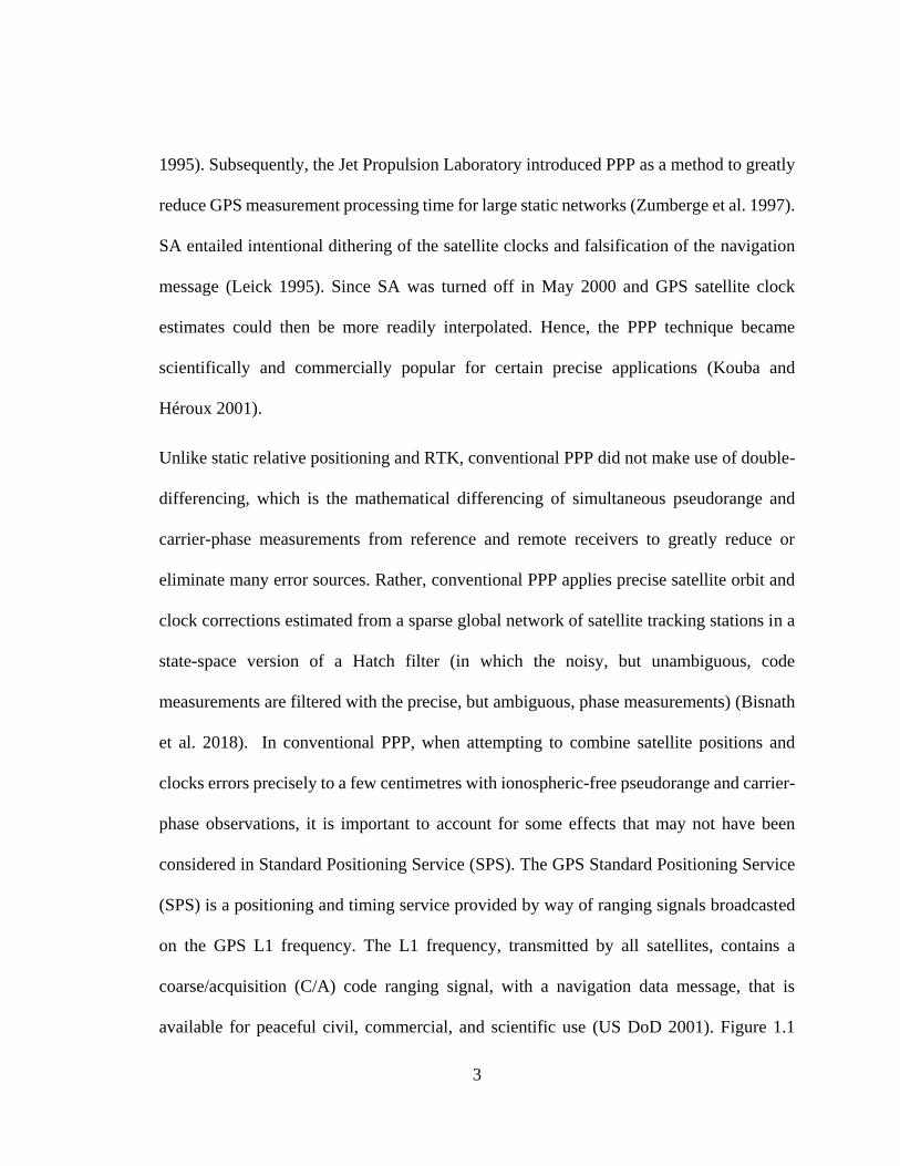
available for peaceful civil, commercial, and scientific use (US DoD 2001). Figure 1.1

4
directly compares the approaches of SPS and PPP. In the SPS, metre-level real-time
satellite orbit and clock information is supplied to the user by each GPS satellite. For single-
frequency users, ionospheric refraction information is also required. For the troposphere a
common mapping function for wet and dry troposphere is utilized (Collins 1999a) in
contrast to PPP that considers different obliquity factors for the wet and dry components
(Seepersad 2012). All of this information is combined with C/A-code pseudorange
measurements to produce metre level user position estimates (Bisnath and Collins 2012).
Where as in PPP, the same receiver tracking information as in SPP is utilized but cm-level
precise orbit and clock information together with additional error modelling and filtering
is utilized to enable dm to mm level user position estimation.
Figure 1.1 Fundamental idea underlying the SPS technique as compared to PPP (Seepersad
and Bisnath 2014a).
Also, defining the PPP error budget becomes more challenging as these error sources can
be subdivided into errors projected onto the range and localized antenna displacements,
illustrated in Figure 1.2. As the signal is transmitted from the satellite to the receiver, error
sources affected in the range domain include satellite and receiver clock error, atmospheric,
relativistic, multipath and noise and carrier-phase wind-up. Antenna displacement effects

5
occur at the satellite and receiver and these include effects such as phase centre offset and
variation, orbit and at the receiver, site displacement effects such as solid Earth tides and
ocean loading. The measurements are continually added in time in the range domain, and
errors are modelled and filtered in the position domain, resulting in reduced position error
in time (Seepersad and Bisnath 2014a).
Figure 1.2 Range to position and time domain transformations in PPP data processing
illustrating the different domains of PPP error sources (Seepersad and Bisnath 2014a).
It is necessary when processing data with a PPP algorithm to mitigate all potential error
sources in the system. As a result of the undifferenced nature of conventional PPP, all
errors caused by the space segment, signal propagation and signal reception directly impact
the positioning solution. Error mitigation can be carried out by modelling, estimating,
eliminated through linear combinations of the measurements or filtering through time
averaging. As previously mentioned, there are additional corrections which have to be

6
applied to pseudorange and carrier-phase measurements such as phase wind-up, antenna
phase centre offset and geophysical effects, in addition to other commonly known effects
such as relativistic correction in order to have a complete observation model in PPP.
Presented in Table 1.1 is a summary of all corrections accounted for and the applied within
the mitigation strategy.
Table 1.1 Summary of error sources in PPP, mitigative strategy and residuals (Seepersad
and Bisnath 2014a)
Effect Magnitude Domain Mitigation method Residuals
Ionosphere 10s m range linear combination;
estimation
few mm
Troposphere few m range modelling; estimation few mm
Relativistic 10 m range modelling mm
Satellite phase
centre; variation
m - cm position;
range
modelling mm
Code multipath;
noise
1 m range filtering 10s cm - mm
Solid Earth tide 20 cm position modelling mm
Phase wind-up
(iono-free)
10 cm range modelling mm
Ocean loading 5 cm position modelling mm
Satellite orbits;
clocks
few cm position;
range
filtering cm - mm
Phase multipath;
noise
1 cm range filtering cm - mm
Receiver phase
centre; variation
cm - mm position;
range
modelling mm

7
Pole tide few cm position modelling mm
Receiver clock 10s m range estimation mm
Atmospheric
loading
cm - mm position modelling cm - mm
Code biases 60 cm range modelling mm
Ambiguity term m - cm range estimation dm - mm
PPP is considered a cost-effective technique as it enables sub-centimetre horizontal and
few centimetre vertical positioning with a single receiver under ideal conditions with few
hours of GNSS data (Seepersad 2012) in contrast to the methods such as relative GNSS,
RTK and Network RTK that require more than one receiver. PPP can be used for the
processing of static and kinematic data, both in real-time and post-processing. PPP’s
application has been extended to the commercial sector, as well in areas such as agricultural
industry for precision farming, marine applications (for sensor positioning in support of
seafloor mapping and marine construction), airborne mapping and vehicle navigation
(Bisnath and Gao 2009). In rural and remote areas where precise positioning and navigation
is required, and no reference stations are available, PPP proves to be an asset. Based on
PPP’s performance, it may be extended to other scientific applications such as ionospheric
delay estimation, pseudorange multipath estimation, satellite pseudorange bias and satellite
clock error estimation (Leandro 2009).
One of the major limitations of conventional PPP has been its relatively long initialization
time as carrier-phase ambiguities converge to constant values and the solution reaches its

8
optimal precision. PPP convergence depends on a number of factors such as the number
and geometry of visible satellites, user environment and dynamics, observation quality and
sampling rate (Bisnath and Gao, 2009). As these different factors interplay, the period of
time required for the solution to reach a pre-defined precision level will vary (Seepersad
2012).
Within academia, industry and governments, there are key areas of focus within the PPP
PPP GNSS measurement processing. These research areas include ambiguity resolution,
integration of PPP and INS, precise atmospheric models, using multi-GNSS constellations
and processing data collected with low-cost (single-frequency) receivers, illustrated in
Figure 1.3. The improvements that these different methods to PPP can be categorized in
terms of reduction of the initial and re-convergence period of PPP and improvement in
solution accuracy.
Figure 1.3: Current research areas in Precise Point Positioning.

9
Review of PPP ambiguity resolution
From the inception of GPS navigation, the largest hindrances to reliable few metre
positioning was a result of the ionosphere delay. As a result of the ionosphere delay, two
L-band navigation signals at 1575.42 MHz (L1) and 1227.60 MHz (L2) were deployed.
After Selective Availability was turned off in 2000, it permitted more precise interpolation
of the satellite clocks. As a result of the more precise modelling of the satellite clock error,
delays due to the ionosphere became more prominent. The ionosphere delay led to the
formation of the ionosphere-free linear combination using GPS data from a single receiver,
as some of the early applications were for post-processing of static geodetic data for, e.g.,
rapid processing of GNSS tracking station data and crustal deformation monitoring.
With the ionosphere delay mitigated using the ionospheric-free linear combination,
conventional PPP’s relatively long convergence time fuelled research in single receiver
ambiguity resolution (AR) (Laurichesse and Mercier 2007; Collins 2008; Mervart et al.
2008; Ge et al. 2008; Laurichesse et al. 2009; Teunissen et al. 2010; Bertiger et al. 2010;
Geng et al. 2012). If the ambiguities could be isolated and estimated as integers, then there
would be more information that could be exploited to accelerate convergence to provide
cm-level horizontal accuracy within an hour of data collection, as illustrated in Figure 1.4.
Resolution of these ambiguities converts the carrier-phases into precise pseudorange
measurements, with measurement noise at the centimetre-to-millimetre level compared to
the metre-to-decimetre-level of the direct pseudoranges (Blewitt 1989; Collins et al. 2010).
Collins et al. (2008) and Laurichesse et al. (2009) saw improvements in hourly position

10
estimates by 2 cm and Geng et al. (2010a) saw noticeable hourly improvements from 1.5,
3.8 and 2.8 cm to 0.5, 0.5, 1.4 cm for north, east and up, respectively.
Figure 1.4: Illustration of the difference between the “float” and “fixed” solution in the
horizontal component. NRC1 DOY 179, 2016 located in Ottawa, Canada.
By 2010, the advantages of PPP ambiguity resolution (PPP-AR) in regards to improved
convergence and position stability was well examined; however, PPP still required over 30
minutes to attain cm-level accuracy (Geng et al. 2010a). During this period, research in
multi-GNSS (GPS and GLONASS) positioning and estimation of slant ionosphere delay
began to exponentially increase. Similar to GPS only PPP-AR, multi-GNSS positioning
resulted in improved convergence time and solution accuracy (Cai and Gao 2007, 2013;
Banville et al. 2013; Li and Zhang 2014; Aggrey 2015). Li and Zhang (2014) showed a
reduction in convergence time from 20 to 11 minutes to attain a predefined threshold of 10
cm 3D. Li and Zhang (2014) and Jokinen et al. (2013) showed the integration of GPS and
GLONASS sped up initial convergence and increased the accuracy of float ambiguity
estimates, which contributed to enhanced success rates and reliability of fixing GPS

11
ambiguities. Estimation of the slant-ionosphere delay permitted instantaneous
convergence, if accurate a priori atmospheric corrections were available to the PPP user
(Geng et al. 2010a; Collins et al. 2012; Banville 2014). Also, if atmospheric corrections
are provided, they assist with improving the reliability of ambiguity-resolved solutions, as
uncertainties of the ambiguities will be lower by more than one order of magnitude (to ~0.2
cy 1𝜎) (Geng et al. 2010a; Collins and Bisnath 2011; Collins et al. 2012; Banville et al.
2014). Naturally, ambiguity resolved triple-frequency was of interest, which promised few
minutes convergence, but also required additional linear combinations to be formed (Geng
and Bock 2013), while it was possible to perform ambiguity resolution of the uncombined
ambiguity terms. The evolution of the PPP user model is presented in Figure 1.5 as the
performance converges to become more RTK-like, primarily due to the ability to perform
ambiguity resolution within the PPP user model and the ability to introduce a priori
atmospheric information.
Figure 1.5: Evolution of the PPP user model.
Over the past decade, each of the GNSSs began modernization efforts. The GPS Block IIF
is now complete, consisting of 12 satellites transmitting on the L5 band and production of
Block III has begun, which will have a 4th civilian signal on L1 (L1C) and promises

12
enhanced signal reliability, accuracy, and integrity. For GLONASS, the third generation
GLONASS-K satellites will change from Frequency Division Multiple Access (FDMA) to
Code Division Multiple Access (CDMA), which will also transmit five navigation signals
on the GLONASS’s L1, L2, and L3 bands. The transition from FDMA to CDMA will
eliminate the Inter-frequency Channel Biases (ICBs), which will allow GLONASS to be
more consistent with other GNSSs, as well as allowing for easier standardization of
GLONASS’s satellite equipment delay products to enable ambiguity resolution. The
European GNSS, GALILEO, is currently under development, with 14 operating satellites
and 4 satellites under commission. Lastly, BeiDou began its transition towards global
coverage in 2015. As of writing, 8 satellites have been launched and they are currently
undergoing in-orbit validation (CSNO TARC 2018).
Within the scope of ambiguity resolution, the five core areas of research that are presented
in Figure 1.6. The core focus within this research is in regard to the publicly available
products that enable ambiguity resolution. Currently, publicly available products are
limited to GPS only. Other research topics such as GLONASS ambiguity resolution and
triple-frequency ambiguity resolution are reviewed in Sections 2.5 and 2.6 respectively.

13
Figure 1.6 Current research areas within PPP ambiguity resolution.
GNSS performance parameters
The performance of any navigation system is characterized by several factors. Some of the
primary factors consists of accuracy, precision, availability, continuity, reliability and
integrity (IMO 2001; Grimes 2007; Porretta et al. 2016). The priority given to these
different factors are application specific. For applications such as, geodetic control
surveying, accuracy is the core requirement (Donahue et al. 2013). Whereas, for safety of
life applications, such as automotive, aeronautical and marine navigation integrity and
reliability is given the highest priority (RTCA DO-181 1983; IMO 2001; European GNSS
Agency 2015). Presented is a review of some of the definitions which have been utilized
within the research presented.
Accuracy and Precision: The accuracy of an estimated or measured position of a navigation
system at a given time is the degree of conformance of that position with respect to a

14
reference position, velocity and/or time (RTCA DO-181 1983; Pullen 2011). Accuracy is
represented as an averaged root mean square (rms) error with respect to the reference
position. Whereas precision represents the standard deviation with respect to the averaged
error or mean. Where error represents the difference between the estimated position and
reference position and mean represents the average of the time period positions were
provided by the navigation system (Anderson et al. 1998).
Availability: The availability of a navigation system is the percentage of time that the
services of the system are usable by the navigator. Availability is an indication of the ability
of the system to provide usable service within the specified coverage area (IMO 2001; U.S.
Coast Guard Navigation Center 2008; Pullen 2011). Non-availability can be caused by
schedule and/or unscheduled interruptions (IMO 2001). The description of availability can
be broken into different components, such as, operational, service, system and signal
availability (Pullen 2011). Where operational availability for e.g. is defined as the typical
or maximum periods of time over which the service is unavailable and service availability
is the fraction of time (expressed as a probability over all satellite geometries and
conditions) that the navigation service is unavailable (Pullen 2011). Renfro et al. (2018)
states there will an operational satellite count availability of ≥ 95% probability that the
constellation will have at least 24 operational satellites. The IGS (2013) states that the
operational availability of their real time products has a 95% availability for their rapid,
ultra-rapid products and real-time products. Presented in Figure 1.7 is an overview of the
availability of each of the contributing analysis centres towards IGS’s Multi-GNSS
Experiment (MGEX). Figure 1.7 highlights the importance of redundancy within a network

15
ensure product availability. Additional information about each of the contributing analysis
centres can be found at IGS (2018a).
Figure 1.7 Multi-GNSS Experiment (MGEX) product availability (IGS 2018a)
Continuity: The continuity of a system is the ability of the total system (comprising all
elements necessary to maintain position navigation system within the defined area) to
perform its function without interruption during the intended operation. More specifically,
continuity is the probability that the specified system performance will be maintained for
the duration of a phase of operation, presuming that the system was available at the
beginning of that phase of operation (U.S. Coast Guard Navigation Center 2008). Presented
by U.S. Coast Guard Navigation Center (2008), the most stringent requirement for the
location determination system to support the Positive Train Control (PTC) system is the
ability to determine which of two tracks a given train is occupying with a probability of
99.999%. The minimum centre-to-centre spacing of parallel tracks is 3.5 m. While GPS
alone cannot meet the specified continuity of service and accuracy, Nationwide Differential
Global Positioning Systems NDGPS (previously called United States Coast Guard DGPS)
in combination with map matching, inertial navigation systems, accelerometers, and other
devices and techniques will provide both the continuity of service and accuracy required

16
to meet the stringent requirements set forth for PTC (U.S. Coast Guard Navigation Center
2017). The IGS (2013) describes the continuity of their ultra-rapid products as 4x daily, at
03, 09, 15 and 21 UTC, daily at 17 UTC for their rapid and continuous for their real time.
Reliability: The probability of success or the probability that the system will perform its
intended function under specified design limits. More specifically, reliability is the
probability that a product will operate within their specifications for a period of time
(design life) under the design operating conditions (such as temperature, volt, etc.) without
failure. In other words, reliability may be used as a measure of the system’s success in
providing its function properly (RTCA DO-181 1983; Pham 2006). Reliability of a system
can be decomposed into failure prevention (robustness and redundancy) and failure
response (resilience). For e.g. the Wide Area Augmentation System (WAAS) focuses on
failure prevention by providing reliability and redundancy to meet the overall National
Airspace System (NAS) requirements with no single point of failure. The overall reliability
of the WAAS signal- in-space approaches 100% (U.S. Coast Guard Navigation Center
2008). Where redundancy is the existence of multiple equipment or means for
accomplishing a given function in order to increase the reliability of the total system (IMO
2001).
A system is considered reliable in terms of robustness if it is resilient with respect to input
and failure uncertainties, and consequently it has low reliability when even the small
amounts of uncertainty entail the possibility of failure (RTCA DO-181 1983). The IGS
also focuses on failure prevention by improving reliability and robustness primarily
through redundancy. IGS products consist of a combination from multiple analysis centres

17
(IGS 2007). As of writing there are 12 analysis centres which contribute towards the
combination of the IGS products (IGS 2018b). By combining multiple products, the
navigation system is less vulnerable to network outages and can maintain availability and
continuity of the service.
Integrity: Integrity is the measure of the trust that can be placed in the correctness of the
information supplied by a navigation system. Integrity includes the ability of the system to
provide timely warnings to users when the system should not be used for navigation
(Ochieng et al. 2003; U.S. Coast Guard Navigation Center 2008; Pullen 2011). Where
integrity risk is the probability of an undetected, threatening navigation system problem
(Parkinson and Axelrad 1988; Ober 1999; Pullen 2011). Overall GNSS system integrity is
described by three parameters: the threshold value or alert limit, the time to alarm and the
integrity risk. The output of integrity monitoring is that individual (erroneous) observations
or the overall GNSS system cannot be used for navigation (IMO 2001). Other definitions
of integrity combine the concepts of reliability and integrity under the title Integrity
Monitoring (Parkinson and Axelrad 1988; Sturza 1988; Feng et al. 2012; Seepersad and
Bisnath 2013; Jokinen et al. 2013a).
Problem Statement
As previously stated, conventional PPP has always required a relatively long initialization
period (few tens of minutes at least) for the carrier-phase ambiguities to converge to
constant values and for the solution to reach the sub-dm-level. This situation is primarily
caused by the estimation of the carrier-phase ambiguity from the relatively noisy

18
pseudoranges and the estimation of atmospheric delay. The result is PPP can then take full
advantage of the precise but ambiguous carrier-phase observations; however, the length of
time it takes to reach the optimal solution is a major disadvantage to the wider use of the
technique. If the underlying integer nature of the ambiguity is known, it can be resolved,
thereby reducing the convergence time of conventional PPP. The challenge of ambiguity
resolution in conventional PPP is due to equipment delays that are absorbed by the
ambiguity state term within the least squares estimation process. These equipment delays
are due to different filters used with the receivers and satellites as well as delays
experienced within the antennas and cables.
To recover the underlying integer nature of the carrier-phase ambiguities, different
strategies for mitigating the satellite and receiver dependent equipment delays have been
developed, and products made publicly available to enable ambiguity resolution without
any baseline restrictions. There has been limited research within the scope of
interoperability of the products which enable ambiguity resolution. Interoperability of the
products can occur within the network solution or within the user solution. The limitation
of product interoperability within the user processing engine is ambiguity re-initialization
due to changing of ambiguity resolution product providers. In addition, there has been no
publish literature examining the performance of product interoperability. If the products
are combined within the network processing engine, this will ensure a continuous precise
user solution if one of the providers experiences an outage. As PPP and PPP-AR is being
adopted by the mass market, which has less stringent accuracy specifications but higher

19
integrity requirements, as a result, a reassessment of the role of ambiguity resolution is
needed.
Thesis Statement
The focus of this research is to develop an effective strategy to improve the reliability of
the PPP ambiguity resolved user solution. Traditionally, PPP users have been expected to
choose between either robust satellite orbit and clock products, which are a combination
from multiple analysis centres or select solutions from individual analysis centre that
provide PPP-AR products. To address the limitation whereby users were expected to
choose between either a robust solution or higher accuracy solution, the following specific
objectives are defined:
1. Implementation of ambiguity resolution of the carrier-phase observable;
2. Re-design of the traditional PPP-AR model to an uncombined representation;
3. Examination of the interoperability of multiple PPP-AR products;
4. Development of a combination process for the PPP-AR products; and
5. Re-examination the role of PPP ambiguity resolution.
Research Contributions
The research presented has been fuelled by the advancements made in ambiguity resolution
by Laurichesse and Mercier (2007); Collins (2008); and Ge et al. (2008). To allow PPP
GNSS measurement processing to be adopted into mass market applications that involves
safety of life for e.g., the operation of autonomous vehicles, there is now increased

20
requirement on the reliability, robustness and integrity of the user solution. To enable
research within the realm of PPP ambiguity resolution it was required to expand of pre-
existing PPP infrastructure to facilitate ambiguity resolution. Presented, is an overview of
the implementation process to enable ambiguity resolution utilizing PPP-AR products.
Receiver dependent equipment delays were mitigated by performing implicit single
(satellite-to-satellite) differencing. Implicit differencing was selected to permit estimation
of the receiver code clock, phase clock and relative carrier-phase L1-L2 measurement
equipment delay. Satellite equipment delays were mitigated by utilizing products from
different public providers to examine performance and interoperability.
PPP users have been expected to choose between either robust satellite orbit and clock
products, which represents a combination from multiple analysis centres or select solutions
from individual analysis centre that provides PPP-AR products. If PPP users selected
combined satellite orbit and clock products they would not be able to resolve the ambiguity
terms as the satellite equipment delays were not mitigated. If the PPP users opted for
products from individual analysis centre that provided PPP-AR products they would be
able to attain a more accurate and precise user solution but be vulnerable to network
outages which is the motivational factor behind the novel research presented. The novel
contributions are comprised of an in-depth analysis of the PPP-AR products in a combined
and uncombined representation, mathematical representation of how to utilize the products
in the different representations, examination of the performance of the PPP-AR products
from different providers, the challenges involved in utilizing the PPP-AR products from

21
the different providers and the strategies required to allow interoperability of the different
products.
As a result of the advancements made in the interoperability of PPP-AR products,
permitted another significant novel contribution, development of a technique to combine
multiple PPP-AR products. The combination of the PPP-AR products resulted in improved
reliability of the user solution and robustness of the products as the user is no longer
dependent on a single analysis centre. Combining of the PPP-AR products will be
performed within the network processing engine which will ensure a continuous precise
user solution
PPP and PPP-AR processing has become routinely utilized within applications such as
crustal deformation monitoring, near real-time GNSS meteorology, orbit determination of
LEO satellites as well as control and engineering surveys where requires few cm-level
positioning accuracy. If PPP-AR is to be adopted in techniques such as lane navigation
which requires 10 to 20 cm horizontal positioning accuracy, a re-examination of the role
of ambiguity resolution in PPP is needed. Within this scope another novel contribution
within this research exists as there has been limited focus on the utilization of ambiguity
resolution as an integrity indicator as having a successfully resolved and validated solution
indicates to the user increased accuracy, precision and reliability of the user solution
thereby increasing the amount of trust that can be placed in the information supplied by the
ambiguity resolved PPP data processing engine.
22
Thesis Outline
Chapter 2 provides an overview of the evolution of the PPP user model over the past two
decades, how to process the measure as well as steps needed to expand the mathematical
model to facilitate ambiguity resolution in PPP utilizing an uncombined representation.
The standard practice in conventional PPP has been to linearly combine two pseudoranges
and two carrier-phases to produce ionosphere-free linear pseudoranges and carrier-phase
combinations which eliminates the first order ionosphere delay. Originally, the ionosphere
delay was considered a nuisance parameter within the positioning community. As a result,
the ionosphere-free linear combination was favoured in contrast to the estimation of the
slant ionosphere delay. Nowadays, the PPP model permits multi-frequency, multi-
constellation, slant ionosphere estimation and ambiguity resolution. Presented in each
section is a review of the steps the PPP user model underwent within its evolution.
Chapter 3 examines the interoperability of high-rate satellite equipment delays which
enable PPP-AR. Interoperability of PPP-AR products is important, as it can increase the
reliability of the user solution while offering similar performance, in regard to precision
and accuracy. Interoperability of the products is possible for the PPP user, as the
mathematical model to enable an ambiguity resolved solution is similar. The different PPP-
AR products contain the same information and would allow for a one-to-one
transformation, allowing interoperability of the PPP-AR products. The PPP user will be
able to transform independently generated PPP-AR products to seamlessly integrate within
their PPP user solution. The seamless integration of the transformed products will allow
the PPP user to have multiple solutions, which will increase the reliability of the solution,

23
for, e.g., real-time processing. During real-time PPP processing, if there were an outage in
the generation of the PPP-AR products, the user can instantly switch streams to a different
provider. A novel component of the research presented is the examination of the
interoperability of PPP-AR products with real data, as well as the presentation of the
products in combined and uncombined representation.
Chapter 4 investigates the feasibility of combining the products from multiple providers of
PPP-AR products. While satellite clock combinations are routinely utilized within the IGS,
they currently disregard the fact that some ACs provide satellite clock products that account
for the satellite equipment delays. Users have been expected to choose either a robust
combined solution or select individual AC solutions that provide PPP-AR products that
allow the user to compute an ambiguity resolved solution. The objective of this
investigation was to develop and test a robust satellite clock combination, while preserving
the underlying integer nature of the clocks and therefore the carrier-phase ambiguities to
the user end to enable PPP-AR. The novelty of the research presented with this chapter is
the development of a process to combine multiple products which enable robust PPP-AR.
Chapter 5 re-examines the role of ambiguity resolution in multi-GNSS PPP with the advent
of quad-constellation, triple-frequency and external atmospheric constraints being
provided to the PPP user. The focus and novelty of this chapter is in the quest to answer
the question: Is ambiguity resolution in PPP needed for accuracy and/or for integrity? First,
a re-examination of the significance between the float and ambiguity resolved PPP user
solution is undertaken. Is the improvement significant enough for applications such as
precision agriculture and autonomous vehicles to justify the additional cost and

24
computational complexity of producing a PPP-AR solution? A novel component within
the realm of PPP-AR is the analysis of ambiguity resolution as a metric to examine the
integrity of the user solution.
Finally, Chapter 6 summarizes all the findings and provides recommendations for research
in the near future.

25
CHAPTER 2 EVOLUTION OF THE PPP USER
MODEL
Over the past two decades, the PPP user model has constantly been evolving. With each
iteration, improvements were made primarily in regards to accuracy and most notably
convergence. The standard practice in conventional PPP has been to linearly combine two
pseudoranges and two carrier-phases to produce ionosphere-free linear pseudoranges and
carrier-phase combinations, which eliminates the first order ionosphere delay. Originally,
the ionosphere delay was considered a nuisance parameter within the positioning
community. As a result, the ionosphere-free linear combination was favoured in contrast
to the estimation of the slant ionosphere delay. Nowadays, the PPP model permits multi-
frequency, multi-constellation, slant ionosphere estimation and ambiguity resolution.
Presented in each of the following sections is a review of the steps the PPP user model
underwent within its evolution.
Introduction into Point Positioning
Single point positioning (SPP), also referred to as absolute positioning or point positioning,
is the most basic GPS solution obtained with epoch-by-epoch least-squares estimation. For
SPP, GPS provides two levels of services, the Standard Positioning Service (SPS) with the
access for civilian users and the Precise Positioning Service (PPS) with the access for the
authorized users. Traditionally, in SPS, only the L1 C/A-code was available. As part of the
modernization efforts, civilians would now gain access to the L2 C/A-code. The achievable

26
real-time SPS 3D positioning accuracy is ~ 10 m at the 95% confidence level. The SPS
model is presented in equation (2.1).
, 1 , 1 1
s s
u u iono tr
s
u C C C opoP dt dt d d + +++= (2.1)
, 1
s
u CP represents the C/A-code modulated on the L1 frequency.s
u is the non-dispersive
delay between satellite ( s ) and user position (u ) including geometric delay. , 1Cudt and 1
s
Cdt
represents the receiver and satellite clock errors, respectively, with respect to GPS time.
ionod and tropod represent the delays caused by ionosphere and troposphere refraction,
respectively.
Conventional PPP model
Similar to SPP, PPP is a positioning technique which only requires a single receiver, but
has the functionality to provide few centimetre-level results in static mode and decimetre-
level results in kinematic mode (Seepersad 2012). To transition from SPP to PPP, two core
components are required:
1) Precise satellite orbits and clocks
Broadcast orbits have an accuracy of ~100 cm in contrast to precise orbits which ranges
from 5 cm, real-time to 2.5 cm, post-processed. The broadcast clocks have a precision of
~2.5 ns in contrast to the precise clocks ranging from ~1.5 ns, real-time to ~20 ps, post-
processed, (Dow et al. 2009).
2) Pseudorange and carrier-phase measurements

27
The pseudorange and carrier-phase measurements are strongly reliant on each other and
are critical to enable precise positioning. The pseudoranges act as a reference frame (or
datum) to the precise but ambiguous carrier-phase measurements. Whereas, the precise
nature of the carrier-phase measurements smooths the relatively noisy pseudorange
measurements.
Presented in equations (2.2) and (2.3) are the pseudorange measurements modulated on the
L1 and L2 frequencies respectively, measured in units of metres. In equations (2.4) and
(2.5) are the carrier-phase measurements modulated on the L1 and L2 frequencies
respectively. The carrier-phase measurements are measured in units of cycles that is
converted to distance. Assuming that PPP related errors such as carrier-phase wind-up,
relativity, antenna phase centre offset and geophysical effects have been properly mitigated
for the observation equations can be written as follows.
1 , 1, 1 , 1 1
s
u P P P
s s s
u u iono tropo P u PP dt dt d d d d + + + + += + (2.2)
2 , 2, 2 , 2 2
s
u P P P
s s s
u u iono tropo P u PP dt dt d d d d + + + + += + (2.3)
, 1 , 1 ,1 1 11 ,
s s s s
u u iono tropo
s
u L L L u L u LLdt dt d d A = + + + + + − + (2.4)
, 2 , 2 ,2 2 22 ,
s s s s
u u iono tropo
s
u L L L u L u LLdt dt d d A = + + + + + − + (2.5)
where ionod represents delays due to ionospheric refraction, tropod represents the delays due
to tropospheric refraction and s
uA is the non-integer phase ambiguity on L1 or L2 in units

28
of metres. d and refer to the equipment delays present within the pseudorange and
carrier-phase measurements, respectively. These equipment delays are due to different
filters used with the receivers and satellites as well as delays experienced within the
antennas and cables (Hauschild and Montenbruck 2014).
To formulate the conventional PPP model, the ionosphere-free linear combination ( IF ) of
the pseudorange ( ,
s
u IFP ) and carrier-phase measurements ( ,
s
u IF ) are formed, which is
presented in (2.6) and (2.7) . In conventional PPP, the ionosphere-free linear combination
is routinely formed because the ionosphere delay is typically considered a nuisance
parameter, thus preferred to be eliminated.
, ,
s
u IF I
s s
u u tropoF IFP dt dt d += ++ (2.6)
, , ,
s s s
u u
s
u IF IF IF utro o IFpdt dt d A +++= + (2.7)
where ,
s
u IFA is the ionosphere-free carrier-phase ambiguity term.
The equipment delays ( , ,, , ,s s
u IF IIF F u IFd d ) were assimilated within the clock terms
( ,,IF
s
Iu Fdt dt ), presented in equation (2.8) and (2.9).
, , ,u u u uIF IF IFdt dt d = + + (2.8)
s s
IF
s s
F IFIdt dt d = + + (2.9)

29
As a result of the unmodelled equipment delays within the satellite and receiver, ,
s
u IFA is no
longer integer natured because the unmodelled equipment delays ( , ,,s s
u IF u IFd ) are absorbed
within the ambiguity parameters (Collins et al. 2010). The implications for not accounting
for these delays are presented in the following equation.
, , , ,
s s s s
u IF IF u IF u IF u IFA N d += + (2.10)
Where ,
s
u IFA represents the real-valued ambiguity
term that is comprised of the integer natured carrier-
phase ambiguity term ( ,
s
u IFN ), which is expressed in
cycles and scaled by the ionosphere-free
wavelength ( IF ) and the equipment delays
( , ,,s s
u IF u IFd ) which are expressed in units metres.
Equation (2.10) and Figure 2.2 illustrates the
importance of accounting for ,
s
u IFd and ,
s
u IF , because
of the co-dependency that exists between the
pseudorange and carrier-phase measurements as a
result of the shared clock terms, also referred to as common clocks ( , ,,F I
s
uI Fdt dt ) (Collins et
al. 2008). If information about the user and satellite equipment delays were accounted for,
the ambiguity term would be integer natured thereby permitting ambiguity resolution. For
the GPS ionosphere-free linear combination, it is not practical to attempt to fix the
Figure 2.1: Conceptual illustration of
the integer nature of the ambiguity
term affected by receiver and satellite
equipment delays.

30
ambiguity term as the wavelength ( IF =0.006 m) is too short relative to the noise of the
linear combination (Collins 1999b). The ionosphere-free observation equations expressed
in (2.6) and (2.7) are presented in equation (2.11) in matrix/scalar form in a combined and
uncombined representation. For simplicity, the troposphere delay, tropod is grouped within
the geometric range, s
u .
1
2
,1
1
1 1
2
,2
,
2
2
2
1 1 1 0 0
0 0 1 1 0 0
0 0 1 1 1 1 0
1 1 0 1
s
us
s
us sIF IF sIF
us sIF IF sIF
us
s
u
pdt
p p
N
N
I
= = −
−
(2.11)
where iu is the frequency dependent coefficient 2
1
2i
i
f
f = .
To recover the underlying integer nature of the carrier-phase ambiguities, different
strategies for mitigating the satellite and receiver dependent equipment delays are
described in the following section.
PPP-AR model
In relative positioning techniques such as RTK, the integer nature of the carrier-phase
ambiguities is uncovered by differencing simultaneous observations from multiple stations
visible to the same satellites. Typically the raw measurements are differenced explicitly
(Leick 1995; Hofmann-Wellenhof et al. 1997). Differencing of simultaneous observations
can be thought of as an optimal correction method (Collins and Bisnath 2011), as the error

31
sources are not modelled. PPP-AR requires the equipment delays within the GPS
measurements to be mitigated, which would allow for resolution of the integer nature of
the carrier-phase measurements (Laurichesse and Mercier 2007; Collins 2008; Mervart et
al. 2008; Ge et al. 2008; Teunissen et al. 2010; Bertiger et al. 2010; Geng et al. 2012;
Lannes and Prieur 2013). These equipment delays are due to different filters used with the
receivers and satellites as well as delays experienced within the antennas and cables
(Hauschild and Montenbruck 2014). Recall equations (2.2) to (2.5) and apply s
uA to the
carrier-phase measurements in equations (2.14) and (2.15) it is shown that by resolving
these ambiguity terms converts the carrier-phases into precise pseudorange measurements,
with measurement noise at the centimetre-to-millimetre level compared to the metre-to-
decimetre-level of the direct pseudoranges (Blewitt 1989; Collins et al. 2010).
1 , 1, 1 , 1 1
s
u P P P
s s s
u u iono tropo P u PP dt dt d d d d + + + + += + (2.12)
2 , 2, 2 , 2 2
s
u P P P
s s s
u u iono tropo P u PP dt dt d d d d + + + + += + (2.13)
1 , 1, 1 , 1 , 1 1
s
u L u L L L
s s s s
u u iono tropo L u LA dt dt d d − = + + + + − + (2.14)
2 , 2, 2 , 2 , 2 2
s
u L u L L L
s s s s
u u iono tropo L u LA dt dt d d − = + + + + − + (2.15)
If the ambiguities could be isolated and estimated as integers, then there would be more
information that could be exploited to accelerate convergence to give cm-level horizontal
accuracy within an hour of data collection. The satellite equipment delays, which are
necessary to resolve the ambiguity terms can be transmitted in two formats. They can be

32
transmitted through an observation space representation (OSR) or state space
representation (SSR). OSR and SSR is a data transmission format for corrections to enable
higher accuracy positioning of a GNSS receiver. OSR corrections are typically utilized in
Network RTK (NRTK) and Differential GNSS (DGNSS), as the range measurements of
the GNSS user are improved by applying a range correction as measured by a nearby
reference station directly to the GNSS measurements. SSR corrections are required for PPP
and PPP-AR, as the assumption when utilizing PPP is, there will not be any localized
infrastructure available to the GNSS user. SSR decomposes the errors into meaningful
states. A network of reference stations is needed to decorrelate the different GNSS error
components (Wübbena et al. 2005). Figure 2.2 illustration of the different correction terms
transmitted in observation space and state space representation. SSR corrections are
preferred in contrast to OSR primarily because it is bandwidth efficient. By decomposing
the range terms into state dependent terms, the state terms can be transmitted at variable
rates such as satellite orbits are transmitted every 30 seconds and satellite clocks
transmitted every 10 seconds (Schmitz 2012).

33
Figure 2.2: Different correction terms transmitted in observation space and state space
representation (Wübbena 2012).
The concept of fixing ambiguities using state space representations was originally
presented in Blewitt (1989), Goad (1985) and Bock et al. (1985). Their research focused
on relative positioning for processing ultra-long baselines, up to 2000 km. Blewitt (1989)
adopted a state space representation where undifferenced measurements in the form of
ionosphere-free linear combinations of the pseudorange and carrier-phase measurements
was processed to form double-differenced estimates. The fractional component of the
satellite equipment delay was needed to enable ambiguity resolution in baseline processing.
Results presented by Bock et al. (1985, 1986, 2000) and Abbot and Counselman (1987)
show improved baseline precision due to ambiguity resolution with the fractional
component of the satellite equipment delay mitigated. Dong and Bock (1989) demonstrated
ambiguity resolution for baseline lengths up to a few hundred kilometres. Note, as the
baseline length increases beyond 20 km, the performance of relative positioning and PPP-

34
AR becomes equivalent (Bertiger et al. 2010), as localized atmospheric errors are no longer
eliminated through double-differencing. Similar performance was noted within the context
of PPP; Ge et al. (2008) saw a 30% improvement in the east component when compared to
the IGS weekly solutions; Collins et al. (2008) and Laurichesse et al. (2009) saw
improvements in hourly position estimates by 2 cm; and Geng et al. (2010a) saw noticeable
hourly improvements from 1.5, 3.8 and 2.8 cm to 0.5, 0.5, 1.4 cm for north, east and up,
respectively.
Traditionally, PPP and RTK has always represented different GNSS processing techniques.
PPP has always been a single receiver data processing technique, utilizing undifferenced
GNSS measurements, while relying on precise orbit and clock with a focus on SSR of error
components. Where as, RTK always required at least two receivers, has been typically
constrained to short baseline (less than 20 km) as a strategy to eliminate localized
atmospheric effects, while enabling ambiguity resolution, with a focus on OSR error
components. The advent of PPP-AR provided the bridging gap between PPP and RTK as
it enabled ambiguity resolution within a single localized GNSS receiver by capitalizing on
correction terms provided from a network of GNSS receivers. In literature, PPP-AR has
sometimes been referred to as PPP-RTK (Wübbena et al. 2005; Teunissen and
Khodabandeh 2015). An appropriate description of the concept PPP-AR is, it is a state
space relative positioning technique, as all error terms are mitigated relative to a global
distribution of receivers. As previously mentioned, to enable PPP-AR, the equipment
delays present within the carrier-phase and pseudorange measurements need to be
accounted for. Currently, there are four common approaches to PPP ambiguity resolution:

35
1. Common Clock model (CC1)
2. Decoupled Clock Model (DCM)
3. Fractional Cycle Biases (FCB) model
4. Integer Recovery Clock (IRC) model
The CC1 adopted an uncombined approach of the measurements, whereas, DCM, IRC and
FCB reformulated the ionosphere-free code and carrier-phase observation equations. The
DCM, IRC and FCB models utilized the Melbourne-Wübbena linear combination (s
MW )
presented in equation (2.16). The Melbourne-Wübbena linear combination is described as
a geometry-free linear combination because the range components are eliminated by
differencing the narrowlane code ( NLP ) and widelane phase ( WL ). The strength of the
Melbourne-Wübbena linear combination is in its ability to isolate the widelane ambiguity
term. Additional details about fundamentals of linear combinations can be found in Leick
(1995), Hofmann-Wellenhof et al., (1997) and Collins (1999b).
1 1
,
2 2
,1
1 1
1 ,1
2
,2
2
2 2
2
1 1 1 0 00 0
1 1 0 00 0 ;
1 1 1 1 0
1 1 0 1
s
us s
s s
IF IF IF u IFs s
s s
IF IF IF us s
MW N
s s
WL uL NL s s
u
s
WL
P PP dt
PI
P
N
N
−
= = − − −
−
(2.16)
As previously mentioned, it is not practical to attempt to fix the GPS ionosphere-free
ambiguity term as the wavelength ( IF =0.006 m) is too short relative to the noise of the
linear combination. As a result of the relatively short ionosphere-free wavelength, ,
s
u IFA is

36
decomposed into the L1 ( ,1
s
uN ) and widelane ( ,
s
u WLN ) ambiguity terms. As a result of the
decomposition of the ,
s
u IFA term, it becomes possible to resolve the ionosphere-free
ambiguity term, equation (2.17). The widelane ambiguity has a wavelength ~86 cm, which
amplifies the ,1
s
uN ambiguity to have a wavelength equivalent to the narrowlane of ~11 cm.
, ,1 ,(17 60 )s s s
u IF IF u u WLNA N += (2.17)
Presented in equation (2.18) are the linear combinations s
IFP , s
IF and s
MW with the
decomposed ambiguity terms 1 ,1
s
uN and ,uL L
s
W WN .
,
1 ,1
,
1 1 0 0
601 0 1
137
0 0 0 1
s
us
IF s
u IFs
IF s
us
s
W
MW
u WLL
Pdt
N
N
=
(2.18)
2.3.1 Receiver equipment delay
When processing undifferenced pseudorange and carrier-phase measurements, the datum
(reference frame) within the adjustment is the pseudorange clocks, as the carrier-phase
measurements are uniquely ambiguous. The receiver clock ( ,IFudt ) is referred to as the
datum, as it is a commonly estimated term between the pseudorange and carrier-phase
measurements, equation (2.16). The datum allows the solution to capitalize on the accuracy
of the pseudorange measurements and precision of the carrier-phase measurements. Collins
(2008) describes the conventional PPP model as sub-optimal in the context of ambiguity

37
resolution, because the estimated ambiguities contain pseudorange and carrier-phase
equipment delays, which degrade the accuracy of the estimated clock parameters.
The first step in enabling PPP-AR requires accounting for the equipment delays generated
by the receiver or changing the datum used for the carrier-phase measurements. The
equipment delays lack unique separation between the clocks and ambiguities, as such, the
solution becomes under-determined.
To remove this singularity, the different PPP-AR techniques adopted implicit (sometimes
incorrectly referred to as “undifferenced”) (Laurichesse and Mercier 2007; Collins 2008;
Zhang et al. 2011) and explicit (Gabor and Nerem 2002; Ge et al. 2008; Bertiger et al.
2010; Geng et al. 2010a; Geng and Bock 2013) single-differencing strategies. Single-
differencing (between two satellites and one receiver) changes the datum of carrier-phase
measurements from the pseudorange clock to the ambiguity terms.
Implicitly differenced observations are closer to the physical observables within the GNSS
receivers, while explicit differencing typically implies differencing of the raw
observations. Ge et al. (2008) differenced the ambiguity terms. Explicit differencing
eliminates the receiver clock and equipment delay, while implicit differencing permits the
estimation of these terms. Implicit and explicitly differenced GNSS observations result in
the same estimates of the desired parameters, as long as the models chosen for the implicitly
differenced (undifferenced) observation biases satisfy the assumptions of the fundamental
differencing theorem. The fundamental differencing theorem states that linear biases can
be accounted for either by reducing the number of observations so that the biases cancel,
or by adding an equal number of unknowns to model the biases. Both approaches give

38
identical results, under certain circumstances. Implicitly differenced observations are
preferred because they permit greater insight into physical and geometrical meaning of the
observable states within the GNSS receiver (Wells et al. 1987).
Presented in equation (2.19) is the implicit differencing strategy adopted within the DCM
and IRC strategies (Laurichesse and Mercier 2007; Collins 2008).
,
,
,
,
1 ,1
1 1 0 0 0 0
601 0 1 0 1
137
0 0 0 1 0 1
s
u
s
u IFs
IF ps
u IFps
IF ps
u WLps
ps
u
ps
WL
MW
u WL
dtP
t
N
N
=
(2.19)
Presented in equation (2.20) is the implicit differencing strategy adopted within the FCB
approach presented in Ge et al. (2008), where the Melbourne-Wübbena combination is
formed independently of the least-squares adjustment and treated as a “correction term”,
thus appearing on the left-hand side of the equation. Fixing of the L1 ambiguity term only
occurs if the fixed widelane is introduced. Fixing of the ionosphere-free ambiguity term
only occurs when both parameters are fixed.
1 ,1 ,
,
1
,
0 1 1 0
1 1 1
s
us
sIF
us ppsWLIF su W p
u
W
u
L u L
Pdt
N NN N
− = −
−
(2.20)
The notation ,1 ,1
s p
u uN N− is used to emphasize the explicit differencing of the ambiguity
terms.

39
2.3.2 Satellite equipment delay
Integer ambiguity resolution of carrier-phase measurements from a single receiver can be
implemented by applying additional satellite (correction) products, where the fractional
component of the satellite hardware delay has been separated from the integer ambiguities
in a network solution (Laurichesse and Mercier 2007; Collins 2008; Mervart et al. 2008;
Ge et al. 2008; Teunissen et al. 2010; Bertiger et al. 2010; Geng et al. 2012; Lannes and
Prieur 2013). The satellite equipment delays or PPP-AR products are typically provided to
the user in two formats, either assimilated within the clocks or provided as a fractional-
cycle phase bias. Presented in Chapter 3 is an examination of each of the public providers
of PPP-AR products.
Slant ionosphere estimation
As mentioned in Section 2.3, with the conventional PPP model, ionosphere-free linear
combination was typically formed as the ionosphere delay was considered as a nuisance
parameter. Capitalizing on the infrastructure built around the conventional PPP model and
expanding on previous literature on ultra-long baseline positioning (Bock et al. 1985; Goad
1985; Blewitt 1989), the Melbourne-Wübbena linear combination was introduced to enable
PPP-AR. The ionosphere-free ambiguity term was decomposed into the widelane and L1
ambiguity terms. With PPP-AR still requiring 10’s of minutes to converge and re-
convergence still problematic, the PPP model was further evolved to permit access to the
slant ionosphere component. The consequence of using ionosphere-free linear
combinations, prevents direct access to the ionosphere component thereby preventing

40
ionosphere constraining. If the slant ionosphere term is estimated, but no a priori
information about the ionosphere is available (no constraints are imposed on the ionosphere
parameters), it is equivalent to the ionosphere-free combination.
Ionospheric corrections generated using a regional or even a global network of stations can
also be beneficial for reducing the convergence time in PPP. There have been two options
discussed in literature for mitigating ionosphere information in the absence of dedicated
reference stations: 1) a peer-to-peer approach, and 2) decomposition of the ionosphere and
utilization of vertical TEC (VTEC) using external sources.
When constraining slant ionosphere delays in the PPP solution, benefits in terms of
precisions are expected if the quality of the external corrections is superior to that of code
noise (Banville et al. 2014). If the a priori estimate of the ionosphere is precise enough,
then ambiguity fixing becomes achievable with only a few minutes of data being collected
which enables cm-level accuracy (Geng 2010; Collins et al. 2012; Li 2012; Ge et al. 2012;
Banville et al. 2014). Availability of slant ionosphere knowledge also allows for quick re-
convergence to ambiguity-fixed solutions following a discontinuity in measurements
(Geng 2010; Collins and Bisnath 2011; Collins et al. 2012), as well as improving
initialization (Ge et al. 2012; Yao et al. 2013; Banville et al. 2014; Lou et al. 2016; Liu et
al. 2017).
In the literature, there are two common approaches that allow ionospheric constraining
while utilizing the ionosphere-free linear combinations. Geng (2010) computed the slant
ionosphere term external to the least-squares adjustment, under the assumption that the
other terms state terms were precisely estimated. Rather than forming the Melbourne-

41
Wübbena combination external of the least-squares solution (equation (2.20)), Ge et al.
(2008) and Geng (2010) formed the widelane linear combination external to the least-
squares adjustment and applied the estimated slant ionosphere as a correction term. The
successfully resolved ambiguity term is introduced as a correction term in a similar
approach as in equation (2.20) with the key difference being the widelane ambiguity term
was resolved faster due to the a priori knowledge of the ionosphere.
Collins et al. (2012) adopted a more formal representation, whereby the estimation of the
slant ionosphere term was included within the least-squares adjustment. To permit the
estimation of the slant ionosphere term, the Melbourne-Wübbena linear combination was
decomposed into its constituents, the narrowlane code and widelane phase as presented in
equation (2.21). The DCM was rebranded into the Extended Decoupled Clock Model
(EDCM). Collins et al. (2012) stated two benefits to processing the widelane and
narrowlane combination simultaneously with the ionosphere-free observables. The first is
that the station and satellite widelane equipment delays can be treated as non-constant,
clock-like parameters identical to the code and phase clocks. Additionally, the least-squares
system is less vulnerable to incorrectly fixed widelane ambiguities biasing the solution.
Residual testing can be used to restart estimation of both the widelane and ionosphere-free
ambiguities if bad fixes on either observable are suspected. Both effects provide for a more
robust solution, with as few a priori assumptions as possible (Collins et al. 2012).

42
,
,
,
1
,
,
2
2 1
1 1 0 0 0 0 0
601 0 1 0 0 1
137
1 0 1 1 0 0
1 0 1 0 0 1
s
u
s
u IFs
psIF
u IFps
psIF
u WLs
NL
p
s
u
WL
u
s
ps
u
ps
WLWL
dtP
t
P
N
I
N
=
(2.21)
The optimality of linear combinations can be defined based on several criteria, such as
noise reduction, ionosphere delay reduction, or wavelength amplification (Collins 1999b).
In recent literature, the role of linear combinations is not clearly acknowledged, as over the
decades, it has become “common knowledge” within the GNSS field. Typically, linear
combinations are formed to reduce the number of parameters to be estimated, thereby
eliminating the terms that are not of interest-nuisance parameters. As previously
mentioned, this is why the ionosphere-free linear combination became the industry
standard over the past two decades, as the ionosphere delay was not of interest within the
positioning community. The pursuit of AR led to introduction of a third linear combination,
then with interest in ionosphere constraining, a fourth linear combination. With the
introduction of multi-GNSS and multi-frequency PPP, some researchers were forming
more linear combinations than the number of underlying measurements (discussed in more
detail in Section 2.6).
At this juncture in PPP’s evolution, it became more intuitive to adopt a more elegant
strategy of processing GNSS data using the raw uncombined observations, where the slant
ionosphere delays are estimated as unknown parameters (Wells et al. 1987; Schaffrin and
Bock 1988; Odijk 2002; Zhang et al. 2011; Li 2012). If mathematical correlations are

43
properly accounted for, it can be shown that combined measurements are equivalent to the
processing of the uncombined measurements (Banville et al. 2014).
Presented in equation (2.22) is the mathematical model used to process dual-frequency
uncombined measurements which is a scalable implementation to utilize uncombined
measurements in the presence of multi-constellations and multi-frequencies.
1
2
1
2
2
2
1
2
12
1
,
,2
1
2
1 ,1
2
1 1 0 0 1 0 0
1 1 0 0 0 0
1 0 1 0 1 1 0
1 0 1 1 0 1
s
u
s
us
ps
us
ps
ps
ups
ps
u
p
u
s
dt dPt
P
N
d
N
I
= + −
−
(2.22)
Within the least-squares solution, it is favoured to present the model in an uncombined
representation as it is easily scalable and the estimated state terms directly represent the
physical observable atmospheric effects and receiver dependent equipment delays. The
benefits of utilizing the combined measurements is primarily due to reduction of the
computational load as well as for simplicity in a priori and a posteriori quality control.
Presented in equations (2.23) and (2.24) are the transformation matrices that can be utilized
to convert measurements, residuals and ambiguities between combined and uncombined
representations.

44
Uncombined to combined:
1
2
1
2
0 0
0 0
0 0
0 0
s sIF IFIF
s sIF IFIF
s s
s sWL
NL NLNL
WLWL
P P
P
p
=
− −
−
(2.23)
Combined to uncombined:
1 2 1
1 2
1 1 2 2
2 12
1 2 11
1 22
1 2 1
2 2
0 0
0 0
0 0
0 0
ss
IF
ss
IF
NL
W
ss
s
L
s
f f f
f f
PP f f f
f fP
f f f P
f f
f f f
f f
−
=
−
−
−
−
+
+
(2.24)
To illustrate the equivalence of the combined and uncombined processing, the P1 and P2
pseudorange residuals are presented in Figure 2.3, in which subplot (a) and (b) are the
residuals of P1 and P2 from the uncombined processing. In Figure 2.3 (c), the residuals were
recombined using the measurement combination co-efficients IF and IF . In Figure 2.3
(d) are the ionospheric-free pseudorange residuals which were produced through
conventional PPP processing. The recombined residuals had a standard deviation of 91.8
cm, where as the ionospheric-free pseudorange residuals from conventional processing had
a standard deviation of 91.9 cm, indicating the equivalence between the uncombined and
combined processing. There is strength in both approaches, such that, in conventional PPP

45
the residuals can be transformed into an uncombined representation to detect faults on a
specific signal.
(a) P1 pseudorange residuals
(b) P2 pseudorange residuals
(c) Combined P1 and P2 pseudorange residuals

46
(d) Ionospheric-free pseudorange residuals
Figure 2.3: Illustration of the residuals for PRN 4 of P1 and P2 pseudorange
measurements, combined P1 and P2 and linearly combined ionosphere-free pseudorange
measurements for the site NRC1 DOY 178 of 2016 located in Ottawa, Canada.
Multi-GNSS PPP
Alongside PPP research into the utility of slant ionosphere estimation, research into multi-
GNSS (initially GPS and GLONASS) positioning was achieving its maturity as
GLONASS re-attained its operational status in October 2011 and the second generation of
BeiDou satellites were launched in 2009, with each successive year new geostationary orbit
(GEO) and medium Earth orbit (MEO) satellites. The benefits of providing the PPP user
with a multi-GNSS solution has always shown its strength in environments such as urban
canyons, mountainous areas and open-pit mines, where the visibility of signals is hindered,
and available signals become contaminated with multipath and noise. The integration of
multiple constellations provides additional independently generated signals, enhanced
satellite geometry and improves the quality of solutions in PPP processing.
Research quantifying the improvements of a multi-GNSS PPP solution is not in short
supply. (2011), Defraigne and Baire (2011), Wang et al. (2012), Cai and Gao (2013), Tu

47
et al. (2013), Choy et al. (2013), Chuang et al. (2013), Li and Zhang (2014), Aggrey (2015)
and Mohammed et al. (2016) all illustrate similar results of initial convergence times being
reduced, but with insignificant improvement in regards to accuracy of the solution after
filter convergence with GLONASS. Cai and Gao (2013) showed improvement in the
position accuracy from GPS-only solutions of 39%, 30% and 60% in the easting, northing
and up components. Even though Choy et al. (2013)’s sample size consisted of only a few
stations, similar results were noted. The performance of the combined GPS and GLONASS
PPP in kinematic mode, showed improvement of 43% and 25% in the horizontal and
vertical components, respectively, and the inclusion of GLONASS did not improve the
accuracy of the converged solution filter. Wang et al. (2012) focused on investigating the
trend and periodic residual characteristic of combined GPS and GLONASS observations.
Their results showed that the positional accuracy of GPS was better than that of GLONASS
by 38 %, 17% and 1% in the northing, easting and up components, respectively. Li and
Zhang (2014) noted that the average convergence time can be reduced by 46 % from 23 to
12 minutes in static mode and by 60 % from 41 to 18 minutes in kinematic mode,
respectively.
As a multi-GNSS solution led to reductions in filter convergence, the next intuitive step
was to look at the contribution of GLONASS in regards to GPS-AR. GPS-AR with float
GLONASS ambiguities was the focus of the research presented by Li and Zhang (2014)
and Jokinen et al. (2013b). Their research showed that the integration of GPS and
GLONASS sped up convergence and increased the accuracy of float ambiguity estimates,
which contributed to enhanced success rates and reliability of fixing ambiguities. Li and

48
Zhang (2014) showed that the average time to the first-fixed solution can be reduced by
27% from 22 to 16 minutes in static mode and by 42% from 34 to 20 minutes in kinematic
mode, respectively. Jokinen et al. (2013b) research showed that on average improvements
were not as significant as Li and Zhang (2014), as the convergence time of GPS-AR only
improved by 5% with the inclusion of GLONASS. Jokinen et al. (2013b) noted that
improvements were dataset dependent, where specific datasets within their sample size
showed improvements as much as 10 minutes.
As discussed in Section 2.3, the primary challenge in PPP-AR relates to the estimation of
the satellite equipment delays within a network of reference stations. While PPP-AR has
been well achieved for GPS, estimation of satellite equipment delays for GLONASS is
difficult because (1) satellites do not share the same frequencies as they are Frequency
Division Multiple Access signals; and even worse, (2) pseudorange hardware biases of
receivers vary in an irregular manner with manufacturers, antennas, domes, firmware, etc.,
which especially complicates GLONASS PPP-AR over heterogenous receivers
(Wanninger 2012).
The addition of the BeiDou, Galileo and GLONASS systems to standard GPS-only
processing reduced convergence time almost by 70%, while the positioning accuracy is
improved by about 25%. Some outliers in the GPS-only solutions were removed when
multi-GNSS observations were processed simultaneous. The availability and reliability of
GPS-only PPP decreases dramatically as the elevation cut-off increases. However, the
availability and reliability of the multi-GNSS PPP is less sensitive and few centimetres are
still achievable in the horizontal components even with 40° elevation cut-off. At 30° and

49
40° elevation cut-offs, the availability rates of GPS-only solution drop significantly to 70
and 40 %, respectively (Li et al. 2015).
Banville (2016b) proposed a strategy which benefited from the frequency spacing of
GLONASS frequencies on the L1 and L2 bands, allowing for an ionosphere-free ambiguity
with a wavelength of approximately 5 cm to be defined; therefore, avoiding the problematic
widelane ambiguity resolution. Based on 12 independent baselines with a mean inter-
station distance of about 850 km over a 1-week period, it was demonstrated that close to
95% of the estimated double-differenced ionosphere-free ambiguities are within 0.15
cycles of an integer, thereby suggesting that long-baseline ambiguity resolution can be
achieved for GLONASS. Applying between station ambiguity constraints was found to
improve longitudinal repeatability in static mode by more than 20% for sessions between
2 and 6 hours in duration. In kinematic mode, only limited improvements were made to the
initial convergence period since the short wavelength of GLONASS ionosphere-free
ambiguities requires the solution to be nearly converged before successful ambiguity
resolution can be achieved.
Geng and Bock (2016) proposed a general approach where external ionosphere products
were introduced into GLONASS PPP to estimate precise FCBs. Geng and Bock (2016)
described the approach as being less impaired by pseudorange equipment delays of
different types of receivers. One month of GLONASS data from 550 European stations
were processed. From a network of 51 inhomogeneous receivers, including four receiver
types with various antennas and spanning about 800 km in both longitudinal and latitudinal
directions, it was found that 92% of all fractional parts of GLONASS widelane ambiguities

50
agreed within ±0.15 cycles with a standard deviation of 0.09 cycles if global ionosphere
maps (GIMs) are introduced, compared to only 52% within ±0.15 cycles and a larger
standard deviation of 0.22 cycles otherwise. Hourly static GLONASS PPP-AR at 40 test
stations can reach position estimates of approximately 1 and 2 cm in rms error with respect
to the reference stations for the horizontal and vertical components, respectively. These
solutions are comparable to hourly GPS PPP-AR. Integrated GLONASS and GPS PPP-AR
can further achieve an rms error of approximately 0.5 cm in horizontal and 1–2 cm in
vertical components. It was noted that the performance of GLONASS PPP-AR across
inhomogeneous receivers depend on the accuracy of ionosphere products (Geng and Bock
2016; Geng and Shi 2017).
Li et al. (2017) examined PPP-AR using the observations acquired from a quad-
constellation, comprised of GPS, BDS, GLONASS, and Galileo (GCRE) utilizing the FCB
approach. The BDS satellite-induced code biases were corrected for GEO, IGSO, and MEO
satellites before the UPD estimation. An average time to first fix (TTFF) of 9 minutes with
7° cutoff elevation angle can be achieved for GCRE PPP AR, which is much shorter than
that of GPS (18 minutes), GR (12 minutes), GE (15 minutes) and GC (13 minutes). With
observation length of 10 minutes, the positioning accuracy of the GCRE fixed solution is
1.8, 1.1, and 1.5 cm, while the GPS-only result is 2.3, 1.3, and 9.7 cm for the east, north,
and vertical components, respectively. When the cutoff elevation angle is increased to 30°,
the GPS-only PPP AR results are very unreliable, while 13 minutes of TTFF is still
achievable for GCRE four-system solutions.

51
Multi-frequency PPP
With a growing number of multi-GNSS satellites available to the GNSS users, there were
also additional signals being made available. The new signals included additional civilian
signals and frequencies. The availability of additional signals and frequencies occurred as
the older satellites are being replaced by the newer satellites with expanded and improved
capabilities. The GPS civilian L2C signal that was introduced with Block IIR-M, provided
dual-frequency capabilities to civilian users. Once L2C becomes fully operational, it will
remove the necessity for codeless or semi-codeless receivers. The availability of a second
civilian signal will open up the GNSS market to other chip manufacturers, increasing
competition in a previously stagnant market, thereby reducing the cost of accuracy
(Leveson 2006). Even more notable is the introduction of the L5 signal, which began
transmitting in May 2010 with the introduction of Block IIF satellites. Some of the benefits
of the L5 signal in contrast to the L1 and L2 includes: improved signal structure for
enhanced performance, higher transmitted power than L1/L2 signal (~3 dB, or 2× as
powerful), wider bandwidth which provides a 10× processing gain, sharper autocorrelation
(in absolute terms, not relative to chip time duration) and a higher sampling rate at the
receiver and longer spreading codes (Leveson 2006).
Planned modernization of GLONASS include an additional signal transmitted on the L5
frequency, and a switch from Frequency-Division Multiple Access (FDMA) to Code-
Division Multiple Access (CDMA), which would increase potential interoperability with
other GNSS. Galileo, the European GNSS, is still under development (De Bakker 2016).
The Galileo system will transmit navigation signals on four different carrier frequencies:

52
L1/E1, L5/E5a, E5b and E6, two of which (E5a and E5b) can also be tracked together as
one extra wide-band (Alt-BOC) signal.
For the three or four frequency carrier-phase measurements case, such as the modernized
GPS, BeiDou navigation satellite system (BDS) and GALILEO, the linear combinations
become much more complicated. Based on the pre-defined extra-widelane (EWL) and WL
linear combinations, Forssell et al. (1997) and Jung et al. (2000) presented the Three Carrier
Ambiguity Resolution (TCAR) method and the Cascade Integer Resolution (CIR) method
for GALILEO and GPS, respectively. Han and Rizos (1999) presented the definition of the
carrier-phase linear combination for the triple-frequency case and discussed the AR
strategies without and with distance constraints by applying the Least-squares AMBiguity
Decorrelation Adjustment (LAMBDA) method to the GF GNSS model. Richert and El-
Sheimy (2007) studied the optimal GPS and GALILEO linear combinations for differential
positioning over medium to long baselines. Feng (2008) introduced the optimal ionosphere
reduced linear combinations for the geometry-based TCAR. Cocard et al. (2008)
systematically investigated the GPS triple-frequency integer phase combinations with an
analytical method and found that the sum of the integer coefficients of the combinations
was an important indicator for systematic classification of sets of combinations. Zhang and
He (2015) examined the BeiDou triple-frequency linear combinations based on the relevant
methods of Richert and El-Sheimy (2007) and Cocard et al. (2008). Hatch (2006) presented
a GF and refraction-corrected method for long baseline AR. Li et al. (2010) also studied
the GF and IF combinations for estimating the narrowlane ambiguity without distance
constraints. Li et al. (2012) presented the optimal triple-frequency IF combination and the

53
GF and IF combination for long baseline AR and precise positioning and shown that the
GALILEO (E1, E6, E5a) has the best performance of long baselines AR, a similar study
that was presented by Wang and Rothacher (2013).
Geng and Bock (2016) used a hardware simulator to generate triple-frequency signals
which were collected with a high-grade receiver to collect 1 Hz data. Measurement noise
and multipath was varied to examine the potential benefit of triple-frequency data under
different conditions. When the carrier-phase precisions on L1, L2 and L5 were set to 1.5,
6.3 and 1.5 mm, respectively, widelane ambiguity resolution attained a correctness rate of
over 99% within 20 s. As a result, the correctness rate of narrow-lane ambiguity resolution
achieves 99% within 65 s, in contrast to only 64% within 150s in dual-frequency PPP. It
was noted that widelane ambiguity resolution was still reliable if the L2 carrier-phase
precision was degraded to 6 mm. For the simulated high multipath data sets with new
ambiguities for all satellites introduced every 120s, it was found that ambiguity-fixed
solutions are achieved at 78% of all epochs in triple-frequency PPP, whilst almost no
ambiguities are resolved in dual-frequency PPP.
Laurichesse and Blot (2016) utilized data from the IGS Real Time service where by
satellite carrier-phase equipment delays were computed for the triple-frequency
measurements. For the test, 10 triple-frequency satellites were in view for the GPS and
BeiDou constellations. A series of widelane-only combinations were formed. By using the
triple-frequency biases, 20 cm accuracy is reached in 2 minutes, compared to 5 minutes
with the use of the dual-frequency biases.

54
Summary of PPP evolution
The standard practice in PPP was to linearly combine two pseudoranges and two carrier-
phases to produce ionosphere-free linear pseudoranges and carrier-phase combinations
which eliminated the ionosphere delay (to the first order). As such, the linear combination
was favoured in contrast to the estimation of the slant ionosphere delay. The PPP model
ionosphere free pseudoranges and carrier-phases is referred to as the conventional PPP
model, which provides the user a float-only (ambiguity unresolved) solution. After, the
PPP model evolved as research begun to focus on mitigating convergence time.
The first step in its evolution was with the research interest in capturing the underlying
integer natured ambiguities. If the ambiguities were isolated and estimated as integers, then
there would be more information that could be exploited to accelerate convergence to
permit cm-level horizontal accuracy. This required expansion of the model to include the
Melbourne-Wübbena linear combination and decomposition of the ionosphere ambiguity
into a widelane and L1 ambiguity with an approximate wavelength of 86.2 and 10.7 cm,
respectively.
With the resolution of the ambiguities, it was soon realized that capturing the integer-
natured ambiguities were not the only key required to unlocking instantaneous cm-level
PPP convergence. As with relative positioning, it was a two-step process. Firstly, it requires
the elimination of the atmospheric terms, which permitted fast convergence of the float
ambiguity term. Secondly it requires the elimination of the hardware delays, which enabled
access to the integer ambiguity term. As a result of the need to access the atmospheric term

55
drove researchers to examine strategies to access the ionosphere term on a software
foundation build around the ionosphere-free linear combination. The easier solution, given
the foundation restrictions, was to decompose the Melbourne-Wübbena linear combination
into its constituents, the narrowlane code and the widelane phase. With a priori slant
ionosphere information being introduced, instantaneous cm-level convergence was
attainable.
With a growing number constellations and frequencies, the foundation built around the
ionosphere-free linear combination needed to be changed, as ad hoc linear combinations
of the measurements were being formed. As this juncture, uncombined measurements were
adopted into the PPP user model, as it facilitated easier scalability in the PPP user
infrastructure. With triple-frequency measurements, improved convergence was noted as
additional knowledge about the ionosphere was made available from a signal with a
stronger transmission. With the introduction of multi-constellations, an abundance of
independent measurements were made available, thereby improving geometry. The
additional measurements allowed faster convergence of the float ambiguity, thereby
improving time to provide an ambiguity resolved solution. Also creating new research in
avenues such as how to select an optimal subset of measurements. Presented in Figure 2.4
is an overview of the described evolution of the PPP user model and presented in Table 2.1

56
is the preferred measurements within YorkU-PPP multi-GNSS and multi-frequency model
for the RINEX 2 and 3 standard.
Figure 2.4: Transition towards the uncombined PPP mathematical model.
Table 2.1: Preferred measurements within YorkU-PPP multi-GNSS model.
GPS GLONASS GALILEO BEIDOU
RINEX
2
RINEX
3
RINEX
2
RINEX
3
RINEX
2
RINEX
3
RINEX
2
RINEX
3
Code
1 P1 C1W P1 C1P C1 C1Z - C1X
2 P2 C2W P2 C2P C7 C8X - C7X
3 C5 C5X - C3X C6 C6X - C6X
Carrier
phase
1 L1 L1W L1 L1P L1 L1Z - L1X
2 L2 L2W L2 L2P L7 L8X - L7X
3 L5 L5X - L3X L6 L6Z - L6X

57
CHAPTER 3 EXAMINATION OF THE
INTEROPERABILITY PPP-AR PRODUCTS
The equivalence in the performance of the different PPP-AR strategies has been shown
extensively in literature with limited focus on integrity and reliability of ambiguity
resolution in PPP. One strategy for improving availability, continuity and reliability is by
allowing the user interoperability of the different providers of PPP-AR products. Examined
within this chapter are the different public providers of the products that enable ambiguity
resolution, the transformations needed to utilize the PPP-AR products in different formats,
analysis of the performance of each of the products and some of the challenges that hinder
interoperability.
Introduction into PPP-AR product interoperability
While the different strategies (FCB, DC, IRC) make different assumptions, there are
fundamental similarities between them. For the PPP user, the mathematical model is
similar; the different PPP-AR products contain the same information and as a result should
permit one-to-one transformations between them, allowing interoperability of the PPP-AR
products (Teunissen and Khodabandeh 2015; Seepersad and Bisnath 2017). The advantage
of interoperability of the different PPP-AR products would be to permit the PPP user to
transform independently generated PPP-AR products to obtain multiple fixed solutions of
comparable precision and accuracy. The ability to provide multiple solutions would
increase availability and continuity, thereby increasing reliability of the solution. For, e.g.,
58
real-time processing: if there were an outage in the generation of the PPP-AR products, the
user could instantly switch streams to a different provider.
The following sections examine the transformation matrix used to transform the combined
(IRC and FCB) products to the DCM format (s
IFdt , s
IFt , s
WN ), as well as the
transformation of all three products to an uncombed observable dependent format ( 1
sd , 2
sd
, 1
s , 2
s ). The novelty of the research presented is focused on the transformation of the IRC
and FCB products to the DCM format which was first published Seepersad and Bisnath
(2015), as well as the performance of the transformed products. Aspects of the
transformation have been published in literature. Laurichesse (2014) focused on the
transformation of the IRC products into an uncombined representation to integrate within
the RTCM SSR standard. Teunissen and Khodabandeh (2015) presented the derivation and
transformation of different models that enables PPP-AR to an uncombined representation.
One of the limitations of the research presented by Teunissen and Khodabandeh (2015)
was the assumption that the IRC and DCM products were identical due to the mathematical
equivalence of the models. Banville (2016a) presented transformations of IRC, DCM and
FCB into an uncombined representation as well. As mentioned by Banville (2016a), one
of the benefits of an uncombined representation, it becomes simpler for the PPP user to
adopt a standardized model to enable PPP-AR. Such a standardized approach also
simplifies the approach of combining multiple PPP-AR products, which would improve
reliability and consistency of the products, is examined in more detail in Chapter 4.

59
For the convenience of the reader, the PPP-AR model from equations (2.21) and (2.22) is
recalled, which illustrates the application of the PPP-AR products in the DCM combined
format, equation (3.1) and the uncombined format, equation (3.2). For simplicity, all
products are transformed into units of metres. The notations used to represent the PPP-AR
products, while relative in nature, is presented utilizing absolute notation as the research
focus is on the user implementation of the products.
Combined representation
2
2 ,1
,
,
1 1 0 0 0 0 01 0 0
601 0 1 0 0 1 0 1 0
1370 1 1
1 0 1 1 0 00 1 0
1 0 1 0 0 1
s
u
us
IF s
ups
IF s
u MWs
NL s
ps
ps
NL u
ps
WL
ps
u
WL
u WL
dtP
t dt
tP
N
N
I
= +
(3.1)
Uncombined representation
1
1
2
12
1
,1 1
2
1 ,1 2
2
2
2
2
,2
1 1 0 0 1 0 0 1 1 0 0 0
1 1 0 0 0 0 1 0 1 0 0
1 0 1 0 1 1 0 1 0 0 1 0
1 0 1 1 0 1 1 0 0 0 1
s
s
u
s
u
us
s
us
ps
ps sups
ps s
u
ps
dt
d
I
dtP
t dP
N
N
= + −
−
(3.2)

60
PPP-AR Products
Currently, there are three main public providers of products that enable PPP-AR. These
include School of Geodesy and Geomatics at Wuhan University (SGG-WHU) (Li et al.
2015; Wuhan University 2017), which provides global post processed FCB products,
Natural Resources Canada (NRCan) (Collins 2008; NRCan 2015), which provides post-
processed DCM products, and Centre national d'études spatiales (Laurichesse et al. 2009;
CNES 2015), which provides post-processed and real-time IRC products. The original
format and units of the products are identified within each of the following sections and all
figures and transformation matrices presented assume the products are in units of metres.
3.2.1 Decoupled clocks
The underlying concept of the DCM presented by Collins et al. (2008) is that the carrier-
phase and pseudorange measurements are not synchronized with each other at the
equivalent levels of precision. The timing of the different observables must be considered
separately, if they are to be processed together rigorously. Also, the decoupled clock
products make no assumption about the temporal variability of the equipment delays,
unlike the other PPP-AR products, as such, they are transmitted in an unfiltered format.
The early DCM was based on ionosphere-free pseudorange and carrier-phase observation
equations, as well as the Melbourne-Wübbena combination: equation (2.19) (Collins
2008). Later, the Melbourne-Wübbena combination was decomposed into the narrowlane
code and widelane phase constituents to facilitate slant ionosphere estimation and
constraining: equation (2.21) (Collins et al. 2010). Both of the models utilized the same

61
DCM products, where reformulation of the model occurred to enable slant ionosphere
estimation and constraining.
Presented in Figure 3.1, Figure 3.2 and Figure 3.3 are each of the three correction terms
that comprise the DCM products. The satellite products consist of carrier-phase clock error
(s
DCMt ), relative code clock offset (s
DCMdt ) and widelane correction ( ,
s
DCM MW ). DCM
products are provided as timing parameters; therefore, s
DCMt is units of seconds and
s
DCMdt and ,
s
DCM MW , which are relative to the phase clocks, are provided in units of
nanoseconds.
Illustrated in Figure 3.1 is the relative satellite carrier-phase clock error (ps
DCMt ) for PRN
28 with respect to satellite PRN 5. “relative” is utilized in this context because of the
explicit differencing of the clock terms between to PRN 28 and PRN 5, which eliminates
the time scale factor because of the reference clock selected by the Analysis Centre (AC).
The linear trend, representing the clock drift, was removed to better illustrate the
underlying clock error.
The satellite code clock offset s
DCMdt represents the difference between the code clock
(s
DCMdt ) and phase satellite clocks (s
DCMt ) is presented in Figure 3.2. s
DCMdt is stored in
units of nanoseconds at a 30 second data rate. The s
DCMdt makes no assumption on the
temporal variability of the equipment delays unlike the other PPP-AR products.

62
Figure 3.1: Relative satellite carrier-phase clock correction provided by NRCan on DOY
178 of 2016 for PRN 28 (relative to PRN 5). Linear trend has been removed. All units are
in metres.
Figure 3.2: Satellite code clock offset provided by NRCan on DOY 178 of 2016 for PRN
28. All units are in metres.
Presented in Figure 3.3 is the satellite widelane correction ( ,
s
DCM WL ) for PRN 28. The
satellite widelane correction is comprised of the code and phase equipment delay as a result
of the Melbourne-Wübbena linear combination formed within the network solution. The
satellite widelane corrections are more stable in time in contrast to the satellite code clock
offset. The DCM also makes no assumptions about the temporal variability of the satellite

63
widelane correction, in contrast to the other providers that treat the terms are daily
constants. ,
s
DCM MW is also stored in units of nanoseconds at a 30 second data rate.
Figure 3.3: Satellite widelane correction provided by NRCan on DOY 178 of 2016 for PRN
28. All units are in metres.
The original YorkU-PPP architecture was designed within the research presented within
Seepersad (2012) and Aggrey (2015). Building on the previously established architecture
from NRCan CSRS-PPP (NRCan 2015), the engine was extended to include the concepts
presented in Collins (2008), as such, code and carrier-phase measurements clocks are
treated independently of each other and implicit single-differencing is performed.
Presented in equation (3.3) is the application of the DCM products to be utilized in the
mathematical model presented in equation (3.1).
1 1 0
1 0 0
0 0 1
ssDCM
ssDCM
sL
sW
tdt
dtt
=
(3.3)
where all units are in metres.

64
Presented in equation (3.4) is the transformation of the DCM products to an observable
dependent representation. The transformation presented in equation (3.4) was also
presented by Banville (2016a). The transformation presented by Teunissen and
Khodabandeh (2015) transforms the DCM/IRC products in phase dependent equipment
delays, where as in equation (3.4) the phase delays are integrated within the common clock
term. In this representation, the satellite clock term (sdt ) is the DCM phase clock, as such
the phase equipment delays (1
and 2
) are zero. The code dependent equipment delays
are present within the s
DCMdt and s
WL terms. The terms s
DCMdt and s
WL need to be
transformed into a code dependent delays, 1
d and 2
d .
1
2
1
2
2
1
1
2 ,
1 0 0
0
0
0 0
0
1
1
0
0 0
s
s
WL DCM
s
DCM
sWL DCM WL
dt f
d f t
d dtf
f
−
=
−
(3.4)
where s s s
DCM DCM DCMdt dt t= −
Presented in Figure 3.4 is s
DCMdt and s
WL for PRN 28 transformed into a code dependent
equipment delay, 1
d and 2
d . Transformation of the productions into a measurement
dependent correction would easily facilitate integration within the Radio Technical
Commission for Maritime Services (RTCM) SSR standard (as discussed in Section 2.3).
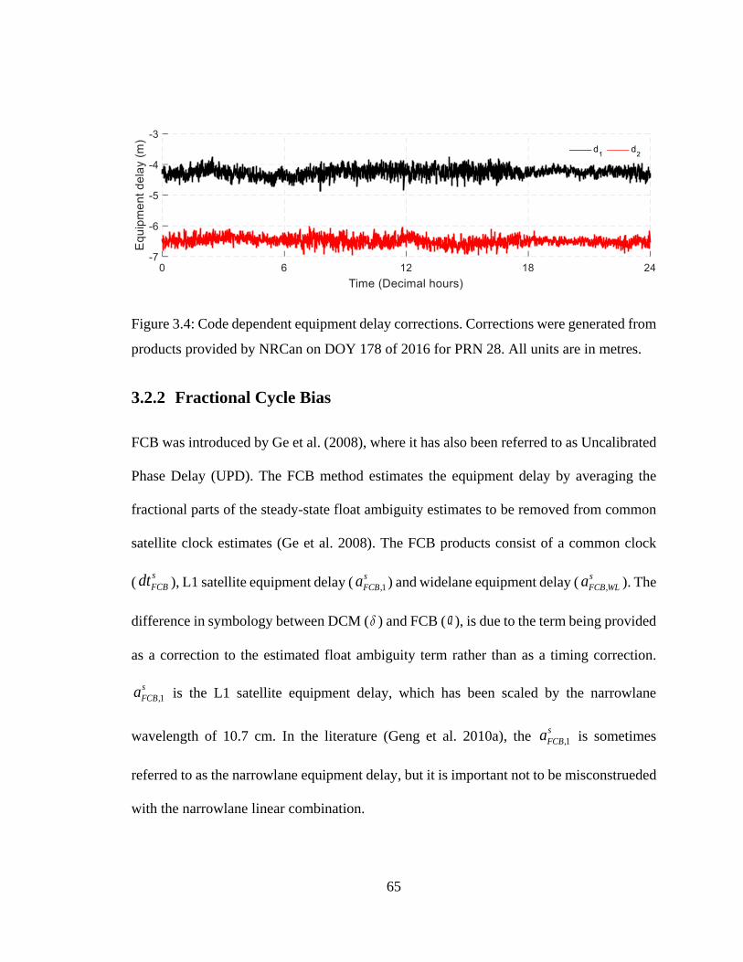
65
Figure 3.4: Code dependent equipment delay corrections. Corrections were generated from
products provided by NRCan on DOY 178 of 2016 for PRN 28. All units are in metres.
3.2.2 Fractional Cycle Bias
FCB was introduced by Ge et al. (2008), where it has also been referred to as Uncalibrated
Phase Delay (UPD). The FCB method estimates the equipment delay by averaging the
fractional parts of the steady-state float ambiguity estimates to be removed from common
satellite clock estimates (Ge et al. 2008). The FCB products consist of a common clock
(s
FCBdt ), L1 satellite equipment delay ( ,1
s
FCBa ) and widelane equipment delay ( ,
s
FCB WLa ). The
difference in symbology between DCM ( ) and FCB (a ), is due to the term being provided
as a correction to the estimated float ambiguity term rather than as a timing correction.
,1
s
FCBa is the L1 satellite equipment delay, which has been scaled by the narrowlane
wavelength of 10.7 cm. In the literature (Geng et al. 2010a), the ,1
s
FCBa is sometimes
referred to as the narrowlane equipment delay, but it is important not to be misconstrueded
with the narrowlane linear combination.

66
Ge et al. (2008), Geng (2010) and Li et al. (2015) opted to provide daily widelane
corrections and lower rate L1 corrections, as the satellite equipment delay were sufficiently
stable in time and space. Geng (2010) describes the widelane satellite equipment delays as
very stable over several days, or even a few months. The widelane FCBs provided by
SOPAC are transmitted once every 48 hours (Geng et al. 2013).
FCB products utilized within this study were obtained from SGG-WHU. Currently SGG-
WHU produces 14 sets of FCB products, corresponding to different precise products such
as those from CODE, ESA, GFZ, GRGS, IGR, and IGS. The FCBs are estimated daily (Li
et al. 2015) when the precise products become available. The FCB products can be
downloaded from ftp://gnss.sgg.whu.edu.cn/product/FCB and have the prefix “SGG” and
the naming convention includes the AC used for generating the FCBs. FCBs generated
using the final IGS products were selected as this set of FCB products capitalized on the
accuracy and reliability of the combined products IGS. Presented in Figure 3.5 is the
relative satellite clock error, psdt for PRN 28 with respect to satellite PRN 5.
Figure 3.5: Relative satellite carrier-phase clock correction provided by Wuhan University
utilizing IGS products on DOY 178 of 2016 for PRN 28 (relative to PRN 5). Linear trend
has been removed. All units are in metres.

67
Presented in Figure 3.6 is the L1 satellite equipment delay, which are provided in units of
cycles at a 15-minute data rate and presented in Figure 3.7 is the widelane satellite
equipment delay, which is also provided in units of cycles but are provided as daily constant
values. The L1 and widelane satellite equipment delays appear smaller in magnitude in
contrast to the DCM products, because the integer component of the delay is removed and
only the fractional component is provided.
Figure 3.6: L1 satellite equipment delay provided by Wuhan University on DOY 178 of
2016 for PRN 28. All units are in metres.
Figure 3.7: Wide lane satellite equipment delay provided by Wuhan University on DOY
178 of 2016 for PRN 28. All units are in metres.

68
To transform the FCB products into a DCM format is presented in equation (3.5)
,1
,
1 0 0
1
0 0
0
ssFCB
ssFCBNL
s sWN FCB WL
dtdt
at
a
=
(3.5)
where, on the RHS and s
FCBdt are in units of metres. ,1
s
FCBa and ,
s
FCB WLa are in units of
cycles. All transformed terms are in units of metres.
Presented in equation (3.6) is the transformation of the FCB products to an observable
dependent representation. In this representation, the satellite clock term (sdt ) is the
common clock term. The equipment delays ( ,1
s
FCBa and ,
s
FCB WLa ) are transformed into a
code dependent delays, 1
d and 2
d . The phase equipment delays (1
and 2
) are set to
zero. The transformed FCB product presented in equation (3.6) is similar to that of the
transformed DCM product such that the phase equipment delays (1
and 2
) are set to
zero. Banville (2016a) and Teunissen and Khodabandeh (2015) transformed the products
to phase equipment delays. Also, Banville (2016a) utilized Differential Code Bias (DCBs)
within the transformation.

69
1
2
1
2
2 2
1 1
,11 1
2 2 ,
1 0 0
0
0
0 0 0
0 0 0
s
s
FCBWL
s
FCB
sWL FCB WL
dt f f
d dtf
d
f
af f
f f a
=
−
−
−
− (3.6)
Presented in Figure 3.8 is the transformation of the FCB products PRN 28 transformed to
code dependent equipment delays, 1
d and 2
d .
Figure 3.8: Uncombined code satellite equipment delay provided by Wuhan University on
DOY 178 of 2016 for PRN 28 using IGS Final products. All units are in metres.
3.2.3 Integer Recovery Clock
The IRC model was first presented by Laurichesse and Mercier (2007). The products by
CNES consists of widelane satellite equipment delays and the carrier-phase satellite clocks.
The widelane satellite equipment delays are estimated as unconstrained in the network
work solution with white noise added at each epoch using the Melbourne-Wübbena
combination. The notable difference between the FCB and IRC approaches is the L1

70
satellite equipment delays are assimilated within the carrier-phase satellite clocks. The
carrier-phase satellite clocks are then aligned to the satellite pseudorange clocks within a
narrowlane cycle. The alignment of the carrier-phase clocks allows the clocks to be used
for the pseudorange and carrier-phase measurements. It is worth noting, real-time
applications would require rigorous quality control to account for the integer offset
between the pseudorange and carrier-phase measurements. As such, it would be more
practical (as with the DCM approach) to allow these integer offsets to exist within the PPP
user solution, rather than it being accounted for in real-time within the network solution.
In 2014, real-time IRC products from CNES were made available in an archived SINEX
BIAS format (Schaer 2016), which consisted of a common satellite clock and a satellite
equipment delays that are provided for each observable (Laurichesse 2014). The IRC orbits
and clocks can be downloaded from IGS, IGN, KASI or CDDIS and the widelane
corrections from ftp://ftpsedr.cls.fr/pub/igsac/. Orbits, clocks and widelane correction files
have the prefix “grg”.
Illustrated in Figure 3.9 is the relative satellite carrier-phase clock error (ps
IRCt ) for PRN
28 with respect to satellite PRN 5 and presented in Figure 3.10 is the widelane satellite
equipment delay, which is also provided in units of cycles but are provided as daily constant
values.

71
Figure 3.9: Relative satellite carrier-phase clock correction provided by CNES on DOY
178 of 2016 for PRN 28 (relative to PRN 5). Linear trend has been removed. All units are
in metres.
Figure 3.10: Wide lane correction provided by CNES on DOY 178 of 2016 for PRN 28.
All units are in metres.
Presented in equation (3.7) is the transformation of the IRC products into a DCM format.
,
,
1 0
1 0
0
s
s
IRC IFs
s
IRC WLsWN
dtt
t
=
(3.7)
where, on the RHS, ,
s
IRC IFt is in units of metres and ,
s
IRC WL is in units of cycles.

72
Presented in equation (3.8) is the transformation of the IRC products to an observable
dependent representation. In this representation, ,
s
IRC IFt the satellite clock term is the
common clock term (sdt ). The P1-P2 differential code biases (
1 2P PB
s
DCd ) was transformed
into code equipment delays ( 1
d and 2
d ). The ,
s
IRC WL is transformed into the phase
equipment delays (1
and 2
) but require the code dependent delays to be removed from
within ,
s
IRC WL . Code delays were introduced into ,
s
IRC WL as a natural effect of forming the
Melbourne-Wübbena combination. An equivalent transformation was presented by
Laurichesse (2014) and Banville (2016a). The DCM/IRC products in Teunissen and
Khodabandeh (2015) where transformed into a similar format of phase dependent
equipment delays but did not utilize the DCBs within their transformation.
1
2 1 2
1
2
,
2
1 ,
1
2
1 0 0
0 0
0 0
0
0
P P
s
IF
s
IRC IFIF
s
IF s
IRC
DC
WL
IF
B
dt
d t
df
f
f
f
d
=
−
− (3.8)
Presented in Figure 3.11 and Figure 3.12 is the transformed IRC products for PRN 28 from
combined to uncombined code and phase equipment delays. The P1-P2 differential code
biases (1 2P PB
s
DCd ) were obtained from the Center for Orbit Determination (2016).

73
Figure 3.11: Uncombined satellite code clock provided by CNES on DOY 178 of 2016 for
PRN 28. All units are in metres.
Figure 3.12: Uncombined satellite phase clock provided by CNES on DOY 178 of 2016
for PRN 28. All units are in metres.
3.2.4 Summary of available PPP-AR products
Presented in this section is an overview of the three main public providers of products
which enable PPP-AR. The criteria examined included the different format of the products
transmitted, data rate and different assumptions made which have been summarized in
Table 3.1. Similar tables were presented in literature over the years (Geng 2010; Shi 2012;

74
Kamali 2017), but have became outdated as research advancements have been made over
the years and refinement of the products presented to the user.
In Table 3.2 is an overview of the transformation matrix that can be used to transform the
different PPP-AR products to the different formats to allow easier integration within the
PPP user’s software format. The table focuses on two types of transformations, 1)
Transforming the different products into the DCM format and 2) Transforming the
combined products into an uncombined measurement dependent format.
Transformation of the different products into the DCM format is novel, as it has only been
published in Seepersad and Bisnath (2015) and Seepersad and Bisnath (2017). The
significance of the work focuses on the integration of the different products within an
infrastructure built around the DCM. Such a transformation addresses any misconceptions
that the AC and PPP user must utilize the same PPP-AR model and products. The PPP user
is allowed to adopt any PPP-AR model and any AR product type as long as consistent error
models are utilized within the AC and the PPP user engine. Also presented are the
transformations to an uncombined measurement dependent representation. Presenting the
products in an uncombined representation is important as it facilitates easier integration
within the RTCM SSR standard and allows the PPP user to adopt any PPP-AR model they
prefer. Such a flexibility would eventually lead to standardization of the PPP-AR user
model.

75
Table 3.1: Comparison of different public providers of products to enable PPP-AR
Fractional Cycle Bias
model
Decoupled Clock model
Integer Recovery Clock
model
PPP-AR
Products
s
IFdt - code clock
,
s
FCB WLa - widelane
,1
s
FCBa - narrowlane
,
s
DCM IFt - phase clock
,
s
DCM IFdt - code clock
,
s
DCM WL - widelane clock
,
s
IRC IFt - phase clock
,sIRC WL - widelane clock
Provided
product units
,sFCB IFdt - seconds
,sFCB WLa - cycles
,1
s
FCBa - cycles
,
s
DCM IFt - seconds
,
s
DCM IFdt - nanoseconds
s
WL - nanoseconds
,
s
IRC IFt - seconds
,
s
IRC WL - cycles
Data rate
sdt - 30 secs
,1
s
FCBa - 15 mins
,
s
FCB WLa - daily
,
s
DCM IFt - 30 secs
,
s
DCM IFdt - 30 secs
,sDCM WL - 30 secs
,
s
IRC IFt - 30 seconds
,
s
IRC WL - daily
General
assumptions
Constant ,
s
FCB WLa are
estimated daily by
averaging arc-dependent
estimates.
No constraints or smoothing
applied
,sIRC IFt aligned to the
satellite pseudorange clocks
within a narrowlane cycle.
,sIRC WL are daily averages.
Products
used Post-processed Post-processed Post-processed
Network
solution
Global.
IGS final products.
Global.
EMR rapid products.
Global.
GRG final products.
NL
correction FCB,1sa
WL
correction ,
sFCB WLa ,
sDCM WL ,
sIRC WL
Source ftp://gnss.sgg.whu.edu.cn
/product/FCB
By request,
nrcan.geodeticinformationse
Orbits and clocks from IGS,
IGN, KASI or CDDIS and
the widelane corrections
from ftp://ftpsedr.cls.fr/pub
/igsac/
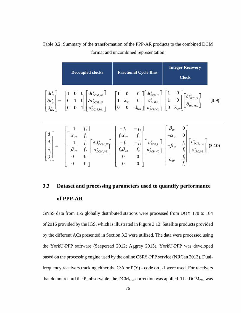
76
Table 3.2: Summary of the transformation of the PPP-AR products to the combined DCM
format and uncombined representation
Decoupled clocks Fractional Cycle Bias
Integer Recovery
Clock
=
s
IF
s
IF
s
WN
dt
t
,
,
,
1 0 0
0 1 0
0 0 1
s
DCM IF
s
DCM IF
s
DCM WL
dt
t
,
,1
,
1 0 0
1
0 0
0
s
FCB IF
s
FCBNL
sWN FCB WL
dt
a
a
,
,
1 0
1 0
0
s
IRC IF
s
IRC WL
WN
t
(3.9)
1
2
1
2
=
d
d
2
1
1 ,
2 ,
1
1
0 0
0 0
WL
s
DCM IF
sWL DCM WL
f
f
f d
f
−
−
2 2
1 1
1 1 ,1
2 2 ,
0 0
0 0
WL
s
FCB
sWL FCB WL
f f
f f
f f a
f f a
− −
− −
1 22
1 ,
1
2
0
0
P P
IF
IFs
IF s
IRC WL
I
C
F
D Bdf
f
f
f
−
−
(3.10)
Dataset and processing parameters used to quantify performance
of PPP-AR
GNSS data from 155 globally distributed stations were processed from DOY 178 to 184
of 2016 provided by the IGS, which is illustrated in Figure 3.13. Satellite products provided
by the different ACs presented in Section 3.2 were utilized. The data were processed using
the YorkU-PPP software (Seepersad 2012; Aggrey 2015). YorkU-PPP was developed
based on the processing engine used by the online CSRS-PPP service (NRCan 2013). Dual-
frequency receivers tracking either the C/A or P(Y) - code on L1 were used. For receivers
that do not record the P1 observable, the DCMP1C1 correction was applied. The DCMP1P2 was

77
utilized when transforming an uncombined representation. DCBs are important to be
accounted for as they represent the systematic errors between two GNSS code observations
at the same or on different frequencies and the signals need to be aligned to IGS’s standard
based on L1-P1/L2-P2 GPS data. The DCBs were obtained from Center of Orbit
Determination in Europe (2016). Dual-frequency uncombined observations were
processed with a priori standard deviations of 1.0 m and 6 mm for pseudorange and carrier-
phase observations, respectively. An elevation cut-off angle of 10° was selected. Slant
ionosphere delays and uncalibrated equipment delays were also estimated epoch-by-epoch
in the PPP filter. The reference stations were analyzed in static mode. Receiver clocks were
estimated epoch-by-epoch. The zenith tropospheric delays were also estimated each epoch
with a random walk coefficient of 2 cm/sqrt(hour). The station coordinates were initialized
using a pseudorange only solution with an initial constraint of 10 m. The IGS absolute
antenna model file was used and ocean loading coefficients were obtained from Scherneck
(2013) for each of the sites processed. To facilitate partial ambiguity resolution, only the
candidates with an elevation angle greater than 20° was considered. The Modified
LAMBDA method (MLAMBDA) was utilized to resolve the ambiguity candidates (Chang
et al. 2005), which is discussed in more detail in Section 5.2. The transformed FCB, DCM
and IRC products were processed with their original satellite orbit files to maintain
consistency between satellite orbits, clocks and equipment delays.

78
Figure 3.13: Global distribution of the selected 155 IGS stations observed during DOY 178
to 184, GPS week 1903, of 2016.
Performance of transformed products
Presented in Table 3.3 is the rms error of the final solution of 24-hour datasets using data
from 155 IGS sites utilizing the satellite products provided by NRCan, CNES, and Wuhan
University. All products were transformed to an uncombined representation. Equivalent
performance (at the few mm level) was noted utilizing the DCM, IRC and FCB products.
Of the three solutions, FCB products had the highest accuracy which is attributed to the
products being generated using final IGS orbit and clock products. To confirm the high
accuracy performance of the FCB products were due to being generated using final IGS
orbit and clock products, the FCBs generated using GRG orbit and clock products were
also examined. The performance of the FCB and IRC products using GRG orbit and clock
products were comparable.

79
Table 3.3: rms error of the final solution produced by YorkU-PPP from 24-hour datasets
using data from 155 sites for DOY 178 to 184, GPS week 1903, of 2016 provided by the
IGS. Satellite products were provided by NRCan, CNES and Wuhan University. All units
are in millimetres.
DCM IRC FCB
Float Fixed Float Fixed Float Fixed
Northing 5 5 5 4 5 4
Easting 6 3 5 3 5 3
Horizontal 8 6 7 5 7 5
Vertical 11 10 11 10 9 9
3D 13 12 13 11 11 10
Data were selected from the GPS site, NRC1 located in Ottawa, Canada on DOY 178 of
2016. NRC1 was selected because similar performance was observed within the week of
processing and it illustrated similar trends to other GPS sites examined. Presented in Figure
3.14 (a) – (c) is the horizontal component and Figure 3.15 (a) – (c) the vertical component
for the IRC, DCM and FCB products. The subplots within Figure 3.14 and Figure 3.15
illustrates both the “float” and “fixed” solution, where fixed represents the ambiguity
resolved solution and float the unresolved solution. A stringent convergence threshold of
5 cm was set to examine the time the solution took to converge.
The horizontal position error, Figure 3.14 (a) – (c) from all three solutions had an overshoot
of 55 – 60 cm after 30 seconds of data processing. Convergence of the float solution to the

80
predefined threshold (5 cm) was 14 minutes and fixing the ambiguities improved
convergence by only 1 minute. Similar convergence was noted in the horizontal component
for all four solutions.
The strength of applying ambiguity resolution is illustrated in the time to attain a steady
state. All three solutions illustrated different convergence trends before attaining a steady
state: DCM products took 2.2 hours, IRC and FCB product took 1 hour. The ambiguity
resolved solution improved the time attain a steady state as the time was reduced to 10
minutes.
The vertical position error, Figure 3.15 (a) – (c), had an overshoot of 36, 45 and 60 cm for
the DCM, IRC and FCB products, respectively. The same predefined threshold for the
vertical component was maintained. Convergence times were 18, 16 and 13 mins for the
DCM, IRC and FCB products, respectively. Applying ambiguity resolution did not
improve the time to attain a steady state in the vertical component: 4.5, 3,5.8 and 2 hours
for the DCM, IRC (GRG), IRC (CNT) and FCB products, respectively. Slower
convergence was noted in the vertical component due the strong correlation between the
atmospheric effects and the vertical component. Any unmodelled components of the
atmospheric effects required time averaging or a priori information to be provided to the
user as discussed in Collins and Bisnath (2011) and Shi and Gao (2014).

81
(a) IRC
(b) Wuhan
(c) DCM
O - Float X - Fixed
Figure 3.14: Site NRC1 DOY 178 of 2016 located in Ottawa, Canada, illustrating the
differences between the “float” and “fixed” solution in the horizontal component where insets
for each figure represents the initial 30 minutes of convergence time. Limits of y-axis represents
position error.

82
(a) IRC
(b) Wuhan
(c) DCM
O - Float X - Fixed
Figure 3.15: Site NRC1 DOY 178 of 2016 located in Ottawa, Canada, illustrating the
differences between the “float” and “fixed” solution in the vertical component where insets for
each figure represents the initial 30 minutes of convergence time. Limits of y-axis represents
position error.

83
Challenges in interoperability of PPP-AR products
Interoperability of the different PPP products is a challenging task due to the public
availability of different quality products, limited literature documenting the conventions
adopted within the network solution of the providers, and unclear definitions of the
corrections. Presented in Table 3.1 was a summary of the different qualities of the products
that were utilized within the study. As mentioned before, ACs are allowed a certain level
of flexibility to improve and innovate through the development of new processing
strategies, such as different axis conventions (Section 3.5.1) and different modelling of
yaw manoeuvres (Section 3.5.2). In the combination process, it is important that the
different strategies (models) utilized by the ACs are taken into consideration within the
user’s estimation process. The general assumption when PPP products are estimated within
the network, assumed that the PPP user will follow similar conventions when utilizing the
products from the network. Consequences of different conventions adopted may result in
incorrect ambiguities being resolved.
3.5.1 Axis convention
For example, IRC adopted the IGS axis convention, whereas the internal DCM products
followed the manufacturer specification. Presented in Figure 3.16 is the orientation of the
spacecraft body frame for GPS Block IIR/IIR-M satellites adopted within the IGS axis
convention, subplot (a), and provided in the manufacturer specifications, subplot (b). The
difference between the manufacturer specifications and IGS axis convention is the
orientation of the X and Y axes.

84
(a) IGS axis convention (b) Manufacturer specifications
Figure 3.16: Orientation of the spacecraft body frame for GPS Block IIR/IIR-M satellites
(a) manufacturer specification system; (b) IGS axis conventions (Montenbruck et al. 2015).
3.5.2 Yaw manoeuvres during satellite eclipse
Another critical component to be accounted for to ensure interoperability of the PPP-AR
products is the difference in the modelling of yaw manoeuvres. Yaw manoeuvres occur
when the actual yaw angle differs from the nominal yaw angle. The nominal yaw angle is
the orientation angle by which a satellite would maintain optimal solar visibility throughout
its orbit, provided it could spin arbitrarily fast. The actual yaw angle is the orientation that
the satellite is able to maintain due to its limited rate of yaw.
All satellites fail to maintain their nominal orientation when their orbits pass close to the
Earth-Sun axis. These are the eclipsing orbits with turns at both orbit noon and orbit
midnight. During a satellite eclipse, Block II GPS satellites behaved unpredictably because
of hardware sensitivity, spinning beyond the nominal amount upon entering the Sun's
shadow. The Block IIR and Block IIF generations of satellites were designed to be able to
maintain their nominal attitude even during orbit noon and orbit midnight (Bar-Sever 1996;

85
Dilssner et al. 2011). For Block IIR, the yaw manoeuvre is constrained by a maximum yaw
rate of 0.2 deg/sec (Kouba 2009) and Block IIF is constrained by a maximum yaw rate of
0.11 deg/sec (Dilssner 2010). The attitude model of the GPS satellites affects the
computation of measurement geometry through variations of the transmitter phase centre
location and carrier-phase measurement wind-up. It also affects the modelling of the solar
radiation pressure force acting on the GPS satellites due to the changes in illumination
geometry (Kuang et al. 2016).
The uncertainty of the yaw manoeuvre is higher during midnight orbit as the satellite
crosses the Earth’s shadow. During the shadow crossing, the satellite’s view of the Sun is
obstructed partially from the region known as the penumbra or fully by the Earth from the
region known as the umbra. A GPS satellite goes through eclipse season approximately
every 6 months and the length of the eclipse season varies from 4 to 8 weeks. A typical
orbit geometry during eclipse season is depicted in Figure 3.17. Eclipse season typically
begins for a GPS satellite when goes below 13.5°, where is elevation of the Sun
above the orbital plane. The time the satellite spends in the Earth’s shadow increases as
approaches 0°, for a time period of up to a maximum of approximately 55 minutes (Bar-
Sever 1996; Kouba 2009; Dilssner et al. 2011). Typically, the nominal attitude model fits
actual GPS measurements well. During eclipsing season when typically goes below 4°,
the physical GPS satellite yaw attitude rate cannot keep up with what is expected from the
nominal model. Dilssner et al. (2011) observed that the orbit noon turn of the Block IIF
satellites manifests in the wrong direction for a small negative angle as much as -0.9°.

86
Figure 3.17: Geometry of an eclipsing satellite, where is elevation of the Sun above the
orbital plane and is the spacecraft’s geocentric orbit angle. “Midnight” denotes the
farthest point of the orbit from the Sun whereas “noon” denotes the closest point. From
Dilssner et al. (2011).
To account for differences in yaw maneuvering during orbit noon and orbit midnight,
knowledge of the actual yaw attitude models from the different ACs is required. As such,
there is a proposal to extend the current RINEX clock format to include additional
information such as yaw angle and phase/code biases (Donahue et al. 2016). The yaw
information would allow for a phase wind-up correction to be applied to each solution for
improved consistency, while the phase/code bias information accommodates the different
PPP-AR products.
Summary of the performance of PPP-AR product interoperability
Interoperability of PPP-AR products is important, as it can increase the reliability of the
user solution while offering similar performance, in regard to precision and accuracy.
Interoperability of the products is possible for the PPP user, as the mathematical model, to
enable an ambiguity resolved solution is similar. The different PPP-AR products contain
the same information and would allow for a one-to-one transformation, allowing

87
interoperability of the PPP-AR products. The PPP user will be able to transform
independently generated PPP-AR products to seamlessly integrate within their PPP user
solution. The seamless integration of the transformed products will allow the PPP user to
have multiple solutions, which will increase the reliability of the solution, for e.g., real-
time processing. During real-time PPP processing, if there was an outage in the generation
of the PPP-AR products, the user can instantly switch streams to a different provider.
The three main public providers of products that enable PPP-AR were examined, which
included School of Geodesy and Geomatics at Wuhan University, Natural Resources
Canada and Centre National d'Etudes Spatiales. Equivalent performance was noted
utilizing the different methods. Of the four solutions, FCB products had the highest
accuracy. The improved performance noted with the FCB products in contrast to DCM and
IRC is attributed to the products being generated using final IGS orbit and clock products
which are a combined product from multiple ACs. Where as, DCM products are generated
using rapid orbit and clocks and IRC products utilize final GRG orbit and clocks. To
confirm the improved performance of FCBs generated from IGS final products, the FCBs
generated using GRG orbit and clock products were also examined and comparable
performance was observed between the FCBs and IRC products.
As the results in Section 3.4 indicated, interoperability of PPP-AR products is feasible.
While feasible, there were challenges when processing the different PPP-AR products.
These challenges were due to the same conventions not being followed between the
network and user solution, for e.g. different satellite antenna convention. When different
satellite antenna convention was used, fractional cycles was introduced when carrier-phase

88
wind-up correction was applied. Another critical component to be accounted for is the
difference in the modelling of yaw manoeuvres. Difficulties in determining the exact
moment when an eclipsing satellite exits the umbra, results in modelling inconsistencies
between ACs. If network-defined periods of orbit noon, orbit midnight and yaw angles are
not provided, it is recommended that the PPP user not attempt to resolve ambiguities of
satellites exiting the umbra if differences in yaw modelling exists between the network and
user.

89
CHAPTER 4 IMPROVING RELIABILITY OF PPP-
AR PRODUCTS
While satellite clock combinations are routinely utilized within the IGS, they currently
disregard the fact that some ACs provide satellite clock products that account for the
satellite equipment delays. Users have been expected to choose between either a robust
combined solution or select individual AC solutions that provide PPP-AR products that
allow the user to compute an ambiguity resolved solution. The objective of this
investigation was to develop and test a robust satellite clock combination, while preserving
the underlying integer nature of the clocks and therefore the carrier-phase ambiguities to
the user end to enable PPP-AR.
Introduction to satellite clock combination
In recent years, CNES, an AC of the IGS, began providing satellite clock corrections
preserving the integer nature of carrier-phase ambiguities. These products are sometimes
referred to as “integer clocks” as they preserve the underlying integer nature of the
ambiguities by including the high-rate satellite equipment delay corrections within the
products. As previously mentioned, utilizing these types of products would allow for PPP
with ambiguity resolution and therefore a more rapid convergence and improved stability
of the position estimates. Other ACs, such as NRCan, also generate such products primarily
for internal use. Even though all IGS ACs follow a set of guidelines and standards to assure
a certain level of consistency, flexibility is allowed to improve and innovate through the
development of new processing strategies (as discussed in Section 3.5). Hence, many ACs

90
utilize their own software packages and methodologies, and all have their solutions based
on an independent selection of ground stations. Theoretically, a combination of the AC
products is not rigorous since solutions are correlated as a result of similar reference
stations used within the network adjustment process. However, on a practical level, given
AC-specific characteristics, a combined solution is more robust against outliers and failures
within individual AC solutions. The strength of a combined product is always in its
reliability and stable median performance, which is better than or equivalent to any single
AC product (Kouba and Springer 2001).
Satellite clock combinations were first proposed by the IGS in 1993 (Springer and Beutler
1993) and became an official product of the IGS starting in January 1994 (Beutler et al.
1995, 1999) as a post-processed product. Real-time or near-real-time products are even
more prone to robustness issues due to unpredictable factors such as communication
outages. The real-time combined product was proposed at the 2002 IGS workshop:
“Towards Real-Time” and the pilot project was launched in 2011 (Caissy et al. 2012).
Satellite clock combinations produced by the IGS currently disregard the integer-
preserving characteristics of the clock products. Users can either opt for the robustness of
the combined solution or select individual AC solutions that provide PPP-AR products,
which allows users to compute an ambiguity resolved solution. The motivation of this work
is to develop and test a PPP-AR clock combination product, improving on the reliability
and robustness of the original products. The following sections consists of a review of the
satellite clock combination process, then the method is extended to include the “integer

91
clock” products, after which the performance of the products are analyzed (Seepersad et
al. 2016).
Satellite clock combination of common clocks
Satellite clock products that do not preserve the integer nature of the ambiguities are
referred to as common clocks (as discussed in Section 2.2). It is well-known that combining
common clock products is an effective method to address the vulnerabilities an individual
AC is susceptible to. In regards to accuracy, the combined clock products have performed
comparable to the products from the best AC solution, (Beutler et al. 1995; Kouba and
Springer 2001), which is expected, as the strength of satellite combination is in improving
reliability and availability of the products and not necessarily accuracy. Clocks can be
combined epoch-by-epoch through weighted least-squares (Weber et al. 2007, 2011) or
combined sequentially using a Kalman or sequential least-squares filter (Mervart and
Weber 2011; Chen et al. 2016).
In the sequential filter approach, clocks estimated by individual ACs are used as
observations (s
adt ) within the adjustment process, where {1... }s m= represents a set of m
number of satellites. Each observation is modelled as a linear function of three parameters:
1) the combined satellite clock (s
dt ); 2) an AC-specific offset ( aB ); and 3) an AC-specific
satellite-dependent offset (s
aA ), where, {1... }a n= is a set of n analysis centres. The
observation equation can be represented as:

92
s s s
a a a a
s
dt dt B A− = + + (4.1)
where s
a is a consistency correction which is time varying and AC specific. s
a aligns the
individual AC solutions to the selected reference frame which, in our case, was defined by
the IGS combined orbit solution. The consistency correction is computed as follows:
( )s s ss a IGS a aa s
IGS
X X D X
X
− − = (4.2)
where s
aX is the AC satellite position vector, s
IGSX represents the IGS combined satellite
position vector, and aD is the geocentre offset vector provided by the respective AC.
Finally, represents the computation of the radius vector with respect to the centre of the
Earth (Ferland et al. 2000; Kouba and Springer 2001).
The term aB in equation (4.1) varies with each AC because of the different timing
constraints imposed on the network. Timing constraints are defined by fixing the clock
parameter of a reference station. Since it is not possible to estimate one such parameter for
each AC, one AC needs to be selected as a timing reference. s
aA varies based on the
different solution-specific ambiguity datum ambiguities and the AC adjustment
constraints. s
aA is unique to each AC and satellite and is considered constant in time. It is
used to model different time references for each satellite within each AC solution. In
practice, s
aA is routinely included as shown in Mervart and Weber (2011) and Chen et al.

93
(2016) in their real-time implementation of satellite combinations of common clocks. s
aA
is included because it absorbs any differently modelled satellite-specific errors. Also,
including s
aA facilitates expanding the satellite clock combination from common clocks to
the clock products that enable PPP-AR. In the sequential filter, s
dt and aB were assigned
an infinite process noise variance whereas s
aA were modelled as constant parameters. Table
4.1 summarizes the different estimated parameters in the satellite clock combination and
associated constraints.
Table 4.1: Estimated parameters in satellite clock combination and associated constraints.
Parameter Description Process
noise
s
dt
Combined
satellite clock
aB Time reference
offset (AC-specific)
s
aA Satellite-dependent
offset (AC-specific) 0
In the adjustment, there is a total of n m m n+ + unknowns and m n measurements and, as
such, there is a rank deficiency of n m+ at the first epoch. To remove this singularity,
different terms were held fixed within the system. As mentioned previously, the timing
reference ( aB ) of one AC must be held fixed. Furthermore, it is required to fix one s
aA

94
parameter for each satellite and AC. Presented in Table 4.2 are the fixed terms in the
adjustment to remove the system’s rank deficiency.
Table 4.2: Fixed terms in the adjustment to remove rank deficiency.
Parameter Fixed terms
Number of
estimated
terms
s
dt 0 m
aB 1 1n −
s
aA 1n m+ − ( ) ( )1 1m n− −
Combining clock products that enable PPP-AR
The previous section discussed the combination process of the common clocks. This
section focuses on the steps required to combine the integer natured satellite clocks
products, DCM and IRC. Rather than transforming the FCB products (as discussed in
Section 3.2) into integer natured satellite clocks, the combined products were compared to
the FCB products. The approach of comparing the combined products to the FCB products
were selected because the FCB products were already generated from IGS combined orbit
and clock products. Therefore, while AR strategies are mathematically equivalent, the
performance of the FCB products surpassed DCM and IRC as a result of this (as discussed
in Section 3.4 as well as illustrated in Figure 3.14 and Figure 3.15). An overview of the
combination process of the DCM and IRC is presented in Figure 4.1, where the first step
requires accounting for AC specific modelling such as different axis conventions and yaw

95
manoeuvres during a satellite eclipse (Section 3.5). Accounting for AC specific modelling
is critical to ensure the integer nature of the carrier-phase ambiguity is not compromised.
The next step combines the widelane products which is followed by the combination of the
clock products that enable PPP-AR.
Decoupled Clocks Integer Recovery Clocks
Account for AC specific modelling
Combine widelane products
Combine integer clocks
Combined clock products that enable PPP-AR
Figure 4.1: Overview of the steps required to combine satellite clocks products that
enable PPP-AR.
4.3.1 Combination process of PPP-AR clock products
The combination process of the integer clocks follows exactly the same parametrization
and constraints, in addition to the integer constraints imposed on the satellite offset. For
the combined products to be integer natured, it is imperative that the reference AC provide
products that enable PPP-AR. Presented in equation (4.3) is the alignment of the widelane
satellite hardware delay for each AC:
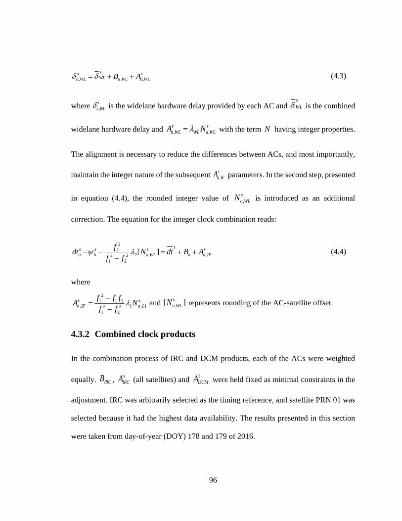
96
, , ,
ss sWLa WL a WL a WLB A = + + (4.3)
where ,
s
a WL is the widelane hardware delay provided by each AC and s
WL is the combined
widelane hardware delay and , ,
s s
a WL WL a WLA N= with the term N having integer properties.
The alignment is necessary to reduce the differences between ACs, and most importantly,
maintain the integer nature of the subsequent ,
s
a IFA parameters. In the second step, presented
in equation (4.4), the rounded integer value of ,
s
a WLN is introduced as an additional
correction. The equation for the integer clock combination reads:
2
2, ,2 2
1 2
2[ ]s
s s s s
a b a WL a a IF
fN B A
fd dt
ft − − = + +
− (4.4)
where
2
1 11
2, , 12 2
1 2
s s
a IF a L
f f fA N
f f
−=
− and ,[ ]s
a WLN represents rounding of the AC-satellite offset.
4.3.2 Combined clock products
In the combination process of IRC and DCM products, each of the ACs were weighted
equally. IRCB , s
IRCA (all satellites) and 1
DCMA were held fixed as minimal constraints in the
adjustment. IRC was arbitrarily selected as the timing reference, and satellite PRN 01 was
selected because it had the highest data availability. The results presented in this section
were taken from day-of-year (DOY) 178 and 179 of 2016.

97
The first component analyzed in this section is the effect of yaw manoeuvres on the clock
combination process. The expectation is that Block IIR and Block IIF satellites are able to
keep their nominal attitude even when orbiting through the penumbra and the umbra.
Because of the difficulties in determining the exact moment of exiting the umbra,
modelling inconsistencies between ACs can be observed. For example, in Figure 4.2, when
PRN 24, a Block IIF satellite, is in the Earth’s shadow, discrepancies are present between
the IRC and DCM products. According to the Jet Propulsion Lab (JPL) within their “.shad”
file (JPL 2016), the time period the satellite transited through the umbra occurred from
03:28:43 to 04:24:09 and 15:27:18 to 16:22:43 and is shaded in green. The limitation of
JPL’s “.shad” file is that only instances of midnight orbits are provided and it does not
include the yaw rate. Highlighted in blue is the information presented in the DCM clock
format, which indicates the time period of a critical yaw manoeuvre within the umbra. In
the DCM clock format, instances of orbit noon are also provided but not illustrated as
consistent modelling occurred during these manoeuvres.

98
Unconstrained AC specific satellite offset
Smoothed AC specific satellite offset
Shadow period provided by JPL
Critical yaw manoeuvre provided by NRCan
Figure 4.2: Inconsistent error modelling during a satellite eclipse for PRN 24 with respect
to PRN 1, Block IIF on DOY 178 of 2016 between IRC and DCM.
Presented in Figure 4.3 is the convergence of the DCM L1 satellite offset. The differences
in yaw manoeuvres and antenna axis convention were taken into consideration. During the
critical yaw manoeuvres the satellite offset of the eclipsing satellite in the DCM solution
was re-initialized.

99
Figure 4.3: Convergence of the forward run of DCM L1 satellite offset with respect to the
IRC on DOY 178, 2016 with the differences in yaw manoeuvres and axis convention taken
into consideration. Each colour represents a different satellite with the integer component
removed from each time series.
As mentioned previously, each AC must adopt a consistent satellite axis orientation
definition. When ignoring the different axis conventions adopted by the DCM and IRC
products, satellite-dependent offsets for the Block IIR/IIR-M satellites converged to 0.5
cycles as opposed to integer values, as illustrated in Figure 4.4.
Figure 4.4: Convergence of the DCM L1 satellite offsets with respect to the IRC for DOY
179, 2016 with the differences in axis convention not account for. Each colour represents
a different satellite with the integer component removed from each time series.

100
Hence, a 0.5 cycle correction term is applied to the measurements for ACs that adopted a
different convention from the IGS. Presented in Figure 4.5 is the consistent integer natured
satellite offset from DCM with respect to IRC on DOY 179, 2016 with an rms error of 0.02
cycles.
Figure 4.5: Convergence of the DCM L1 satellite offset with respect to the IRC on DOY
179, 2016 with the differences in axis convention account for. Each colour represents a
different satellite with the integer component removed from each time series.
Figure 4.6 illustrates an example of the estimated widelane DCM satellite offset with
respect to the IRC solution on DOY 178, 2016. Each line represents one satellite with the
integer component removed. The final estimates of have an rms error of 0.03 cycles.

101
Figure 4.6: Convergence of the DCM widelane satellite offset with respect to the IRC on
DOY 178, 2016. Each colour represents a different satellite with the integer component
removed from each time series.
Presented in Figure 4.7 is the time reference parameter of the DCM solution ( DCMB ). Since
the term was fixed, this offset effectively represents the offset between the DCM and IRC
timing references.
Figure 4.7: Time reference parameter of DCM with respect to IRC on DOY 178, 2016.
Post-fit residuals of the combined IRC+DCM clock with respect to the IRC clock products
for DOY 178, 2016 is presented in Figure 4.8 with an rms of 0.42 cm, where 98.85% of
the residuals were within 1 cm.

102
Figure 4.8: Post-fit residuals of the combined clock (IRC and DCM) with respect to the
reference clock (IRC) on DOY 178, 2016.
Aligning IGS common clocks to clock products that enable PPP-
AR
As a proof of concept, IGS common clocks were also aligned the IRC integer clocks to
allow for ambiguity resolution with the (re-aligned) IGS clocks. Similar to the DCM and
IRC combination, IRCB , s
IRCA (all satellites) and 1
IGSA were held fixed as minimal constraints
in the adjustment. An infinite weight was assigned to the clocks provided by the IGS, and
hence the combined clocks maintain the time variation of the IGS clocks. By assigning an
infinite weight and combining the clocks relative to an integer clock solution, the combined
clock product has the precision and stability of the original IGS common clocks, while
preserving the integer nature of the ambiguities at the user end. Presented in Figure 4.9 is
the forward run of the IGS L1 satellite offset estimation with respect to the IRC clocks on
DOY 178, 2016. As expected, because the IGS clocks are a combined common clock,
satellite offsets are real-valued. Presented in Figure 4.10 is the time reference offset of IGS
with respect to the IRC solution. Post-fit residuals of the combined IRC+IGS clock with

103
respect to the IRC clock products on DOY 178, 2016 is presented Figure 4.11 with an rms
of 0.3 cm, where 99.92% of the residuals were within 1 cm indicating the similarity in
performance of IRC and IGS clock products.
Figure 4.9: Convergence of the forward run of IGS L1 satellite offset with respect to the
IRC on DOY 178, 2016. Each colour represents a different satellite with an integer
component removed from each time series.
Figure 4.10: Time reference parameter of IGS with respect to IRC on DOY 178, 2016.

104
Figure 4.11: Post-fit residuals of the combined clock (IRC and IGS) with respect to the
reference clock (IRC) on DOY 178, 2016.
Performance of combined satellite clock products
The goal of this section is to evaluate the quality of satellite clock combinations that enable
PPP-AR in the position domain. The performance was assessed utilizing the same dataset
described in Section 3.3 which was comprised of multi-GNSS data from 155 globally
distributed stations from DOY 178 to 184 of 2016. Float ambiguity PPP solutions
computed with the IGS clocks, (labelled ‘IGS’) and PPP-AR solutions obtained with the
CNES IRC products (labelled ‘IRC’) are compared. Two sets of combined products are
also included in the evaluation: 1) combined satellite clock products that enabled PPP-AR,
labelled as ‘IRC+DCM’ and, 2) The aligned IGS clocks to permit PPP-AR, labelled as
‘IGS-AR’. A summary of the different products which are being combined from IGS,
CNES and NRCan are presented in Figure 4.12. Also included are the FCB products,
labelled ‘IGS-FCB’ which were reviewed in Section 3.2.2 and the performance was
analyzed in Section 3.4. As previously discussed, this set of FCB products was generated
utilizing the final IGS products.

105
Figure 4.12: Overview of analysis centres used to generate combined products IGS-AR
and IRC+DCM
In static mode, position repeatability over the 7 days processed was examined. For each
station, the standard deviation of the 7 daily estimates for the northing, easting and up
components was computed. These repeatability measures were then averaged over all
stations to yield the results presented in Figure 4.13. This process was repeated for every
satellite clock product investigated. The impact of ambiguity resolution can clearly be seen
in the easting component, where all solutions with ambiguity resolution outperform the
standard IGS clock solution in terms of the easting repeatability. Aligning the IGS clocks
to the IRC clocks has produced the best solutions, suggesting a benefit from both the
robustness of the IGS combination and the integer properties of the integer clocks. Finally,
the IRC+DCM solution provides repeatabilities that are marginally better than the IRC
solution at the few mm-level. Also, as expected the IGS-FCB products performed similar
to the IGS-AR products as they benefited from the robustness of the IGS combination.

106
Figure 4.13: Examination of the repeatability of the PPP user solution in static mode
utilizing different types of clock products. Statistics are based on GPS data from 155 IGS
stations were observed during DOY 178 to 184, of 2016. All units are in millimetres.
Similarly, Figure 4.14 presents the results for kinematic processing. A different evaluation
scheme was used in this case: for each daily station processing, the standard deviation of
the latitude, longitude and height components were computed. The values for all 155
stations over the 7 days were then ordered and the 90th percentile values were extracted.
This method was adopted as solution resets within the day (due to data gaps for example)
can impact the mean value. Similar conclusions as in the static case can be made, where
the contribution of ambiguity resolution significantly improves the solution. In this case,
aligning the IGS clocks to the IRC clocks offered only marginal benefits over the original
IRC solution.
0
1
2
3
4
5
Northing Easting Up
Ave
rage
Rep
eata
bili
ty (
mm
)
IGS IRC IRC+DCM IGS-AR IGS-FCB

107
Figure 4.14: Examination of the repeatability of the PPP user solution in kinematic mode
utilizing different types of clock products. Statistics are based on GPS data from 155 IGS
stations were observed during DOY 178 to 184, of 2016. All units are in millimetres.
Summary of the benefits of combining AR products
The satellite clock combinations routinely produced within the IGS currently disregard that
ACs provide products which enable ambiguity resolution. Users have been expected to
choose either an IGS product which is a combined product from multiple ACs or select an
individual AC solution which provides products that enable PPP-AR. The goal of the novel
research presented was to develop and test a robust satellite clock combination preserving
the integer nature of the carrier-phase ambiguities at the user end.
For a satellite clock combination to provide an integer-aligned clock, it is important that
the different modelling utilized by the ACs are properly considered in the adjustment
process. Two different types of modelling were addressed, namely: 1) different satellite
0
10
20
30
40
50
Northing Easting Up
Ave
rage
Rep
eata
bili
ty (
mm
)
IGS IRC IRC+DCM IGS-AR IGS-FCB

108
axis conventions, and 2) differences in modelling of yaw manoeuvres. By not accounting
for these differences in the combination process, the underlying integer nature of the clock
products were compromised.
For GPS Block IIR/IIR-M satellites, the IGS axis convention and manufacturer
specifications are not equivalent. The difference between the two axis representations for
Block IIR/IIR-M satellites is the orientation of the X and Y axes. To account for the
differences in antenna conventions, a 0.5 cycle correction term must be applied to the
clocks for ACs that adopted a different convention from the IGS.
Different ACs have adopted different standards for modelling the yaw manoeuvres during
orbit noon and orbit midnight. To account for the inconsistent yaw modelling between ACs.
It is critical that additional information such as yaw angle and phase/code satellite hardware
delays are provided at the same intervals as the clocks. The yaw information would allow
for a phase wind-up correction to be applied to each solution for improved consistency,
while the phase/code satellite hardware delays accommodates different product
representations, such as FCB. To this end, an updated RINEX clock format is suggested.
Two sets of combined clock products were generated: 1) combined satellite clock products
that enable PPP-AR, and 2) IGS satellite clocks aligned to enable PPP-AR. The combined
products were evaluated in the position domain by processing GPS data from 155 IGS
stations, observed during DOY 178 to 184 of 2016. mm-level differences were noted,
which was expected as the strength lies mainly in its reliability and stable median
performance and the combined product is better than or equivalent to any single AC’s
product in the combination process. Aligning the actual IGS satellite clock products yielded

109
the best PPP-AR results, for both static and kinematic solutions, where mm-level
improvements were noted.

110
CHAPTER 5 REASSESSING THE ROLE OF
AMBIGUITY RESOLUTION IN PPP
With the advent of quad-constellation, triple-frequency and external atmospheric
constraints being provided to the PPP user, the novelty and focus of this chapter is in the
quest to answer the question: Is ambiguity resolution in PPP needed for accuracy or for
integrity? To determine if ambiguity resolution in PPP for accuracy or for integrity an
examination of the significance between the float and ambiguity resolved PPP user solution
is undertaken. Assessment of ambiguity resolution as an integrity indicator has also been
an area that has lacked attention. Is the improvement significant enough for applications
such as precision agriculture and autonomous vehicles to justify the additional cost and
computational complexity of producing a PPP-AR solution?
Introduction
The utilization of ambiguity resolution in PPP has been primarily focused on high accuracy
applications such as geodetic surveying. To re-examine the role of ambiguity resolution in
PPP, accuracy specifications from precision agriculture and autonomous vehicles is
assessed to determine if the improvement in accuracy between float and resolving GPS
ambiguities is significant (Seepersad et al. 2017). Results consist of solution analysis of
convergence time (time to a pre-defined performance level), position precision
(repeatability), position accuracy (solution error with respect to analysis centre’s weekly
SINEX solution) and residual analysis. Pre-defined thresholds are based on specifications
for lane navigation and machine guidance for agriculture.

111
A novel component within the realm of PPP-AR is the analysis of ambiguity resolution as
a metric to examine the integrity of the user solution. Integrity within the context of the
PPP user solution means, the amount of trust that can be placed in the information supplied
by the PPP data processing engine. Integrity also relates to the PPP engine’s ability to
provide timely warnings to users when the solution should not be trusted. Given that in
PPP processing, all parameters must be accounted for without multiple solutions (as is in
the case with double-differenced static, multi-baseline networks and network RTK),
providing integrity information for PPP single receiver estimates is all that more important.
Within the context of integrity monitoring, ambiguity resolution will be further examined.
The role of ambiguity resolution depends on what are the user specifications. If the user
specifications are at the few cm-level, ambiguity resolution is an asset, as it improves
convergence and solution stability. Whereas, if the user’s specification is at the few dm-
level, ambiguity resolution offers limited improvement over the float solution. If the user
has the resources to perform ambiguity resolution, even when the specifications are at the
few dm-level, it should be utilized. To have a high probability of correctly resolving the
integer ambiguities, the residual measurement error should be less than a quarter of a
wavelength (Georgiadou and Kleusberg 1988; Banville 2014; Petovello et al. 2014).
Having a successfully resolved and validated solution can indicate to the user increased
accuracy, precision and reliability of the user solution thereby increases the amount of trust
that can be placed in the information supplied by the ambiguity resolved PPP data
processing engine.

112
Ambiguity resolution
Ambiguity resolution in PPP requires the equipment delays within the GNSS
measurements to be mitigated, which would allow for resolution of the integer nature of
the carrier-phase measurements. Resolution of these ambiguities convert the carrier-phases
into precise pseudorange measurements, with measurement noise at the centimetre-to-
millimetre level compared to the metre-to-decimetre-level of the direct pseudoranges. If
the ambiguities could be isolated and estimated as integers, then there would be more
information that could be exploited to accelerate convergence to give cm-level horizontal
accuracy within an hour of data collection.
5.2.1 Partial Ambiguity resolution
In multi-constellation processing, low elevation satellites will be frequently tracked. These
low-elevation ambiguities suffer much more from observation noise, multipath effects and
the residual atmospheric delays, and thus have much lower accuracies. Therefore, the
likelihood of correctly fixing all ambiguities simultaneously is low. If all ambiguities are
fixed simultaneously, the low-elevation ambiguities may influence the search system and
make the search result unable to pass the acceptance test.
The challenge of partial ambiguity resolution is finding the largest possible subset of the
reliable ambiguities. As a result, different sorting methods have been proposed to fix the
largest possible subset of the ambiguities with bootstrapping method. Bootstrapping is a
statistical method that resamples the ambiguity candidates to estimate the ambiguity
resolved user solution. A partial decorrelation can be applied before the partial ambiguity

113
resolution to improve the success-rate (Teunissen 2005; Henkel and Günther 2010). The
challenge in partial ambiguity resolution is determining the largest possible subset of the
reliable ambiguities. Some conventional techniques of the ambiguity subset selection are
Sequential fixing Ascending Variance Order (SAVO), Sequential BLewitt fixing Order
(SEBLO) method, Sequential Optimum Fixing Order Search (SOFOS) method, and Batch
partial ambiguity resolution (Henkel and Gomez 2013; Kamali 2017).
A common approach is the SAVO method (Teunissen 1998), in which float ambiguities
are ordered based on their precision. A subset of the most precise is validated first and if
the successfully resolved the set of candidates are validated. The remaining subsets of
ambiguities with lower precision are bootstrapped. The sequential fixing continues until
reaching the ambiguity that can no more be fixed to its nearest integer value. All
combinations of independent subsets of ambiguities are then tested, maximizing the
number of fixed ambiguities.
There were also more simplistic approaches such as a decision to fix is made when both
the formal sigma and the fractional component of the float ambiguity drops below a
common threshold. During the early developmental period of PPP-AR, researchers
recommended different thresholds such as 0.15 cycles (Collins et al. 2010) and 0.2 cycles
(Geng et al. 2010a). The concept of these thresholds was, if the fractional component of
the ambiguity term were within a threshold, it would lead to a correctly resolved ambiguity
solution. Within the scope of this research, a threshold based only on the elevation angle
of the satellite was selected. An elevation threshold of 20° was selected as this elevation
cut-off angle was determined as optimal based on multipath analysis presented in

114
Seepersad and Bisnath (2014b), where typical ground bounce multipath observed with a
geodetic GNSS antenna, was pronounced at elevation angles less than 20°. To ensure
reliable ambiguity resolution, the error budget should remain below a quarter of a
wavelength, namely 10 cm / 4 = 2.5 cm for the ionospheric free combination (Banville
2014).
5.2.2 Resolving and fixing the ambiguities
When determining the integer candidates for an ambiguity resolved solution, there are
several different approaches that have been utilized over the decades, these include
Cascade Integer Resolution, Fast Ambiguity Resolution Approach (FARA), Fast
Ambiguity Search Filter (FASF), Least-squares AMBiguity Decorrelation Adjustment
(LAMBDA), Least-Squares Ambiguity Search Technique (LSAST), Optimal Method for
Estimating GPS Ambiguities (OMEGA) and Three Carrier Ambiguity Resolution (Kamali
2017). The de facto standard for determining the integer candidates has become the
LAMBDA method because of its high success-rate is based on integer least-squares, of
which optimality has been proven, that is, highest probability of success. In TCAR and
CIR pre-defined ambiguity transformation are used, whereas LAMBDA exploits the
information content of the full ambiguity variance-covariance matrix, with statistical
decorrelation the objective in constructing the ambiguity transformation. For resolving the
ambiguities, TCAR and CIR were designed for use with the geometry-free model.
LAMBDA can inherently handle any GNSS model with integer ambiguities and thereby
utilize satellite geometry to its benefit in geometry-based models (Teunissen et al. 2002).

115
The concepts of LAMBDA would not be discussed in further detail here as it has been well
documented in literature (Leick 1995; Hofmann-Wellenhof et al. 1997; Teunissen and
Kleusberg 2012). To improve the computational deficiencies of LAMBDA, Chang et al.
(2005) developed modified LAMBDA (MLAMBDA). MLAMBDA improved the
computational speed of LAMBDA, which becomes critical for real-time, multi-GNSS,
triple-frequency positioning. The MLAMBDA routine utilized within the PPP engine was
obtained from the open source program package RTKLIB (Takasu and Yasuda 2009). The
inputs to the MLAMBA function requires the float ambiguity estimates, covariance of the
ambiguity terms and the number of sets of integer ambiguities to be returned. The output
of the function consists of the number of specified sets of integer ambiguities and the sum
of squared residuals of each set of integer ambiguities.
After resolving the ambiguities, there are two main approaches for determining the
ambiguity resolved position estimates. These can be performed either functionally (De
Jonge and Tiberius 1996) or stochastically (Euler and Schaffrin 1991; Wang et al. 1998).
While both approaches are equivalent, the approach by Euler and Schaffrin (1991)
presented in equation (5.2) was adopted because it was more flexible from a programming
perspective.
Ambiguity resolution can be thought of as a three-step process. After the least-square
estimation, the vector of unknown parameters ( x ) are sorted according to their meaning
utilizing a permutation matrix (Henderson and Searle 1981). The first part consists of all
the non-ambiguity terms (e.g., coordinates, clock terms and atmospheric terms), which is

116
represented by 1x and the float ambiguity terms are represented by 2x in equation (5.2).
After, float ambiguity candidates with the highest likelihood to be successfully resolved
are determined and these float ambiguity candidates are constrained utilizing a Boolean
matrix ( K ). K is comprised only of 0’s and 1’s, where the corresponding candidates to be
resolved are assigned a 1. For a total number of ambiguity candidates ( r ) and a number of
integer candidates to be fixed ( f ), the constraints to be formed is presented in equation
(5.1).
K= 0, rI (5.1)
Where 0 = zero matrix ( ( ))f u f − , rI = boolean matrix ( )r f and u is the total
number of unknown parameters.
The K matrix allows for constraints to be imposed on a solution after estimation without
constraints on the ambiguity parameters, thereby easily permitting epoch-by-epoch fixing.
The underlying float solution is maintained independently with the ambiguity-fixed
solutions computed separately, as illustrated in Figure 5.1. Epoch-by-epoch fixing is an
optimum way of combining sequential least-squares filter with integer state estimation, as
well as maintain an independent float solution for comparison purposes. The main benefit
of this approach is that the float solution remains uncorrupted by possibly incorrect
ambiguity fixes. The downside of epoch-by-epoch fixing is the increased computational
load when combined to permanently fixing ambiguity candidates. Permanently fixed

117
ambiguity candidates allow for reduction of matrix sizes as they are no longer included in
state terms and covariances.
Figure 5.1: Schematic approach to fixing (Collins et al. 2010).
The final step after resolving the ambiguities, involves applying the ambiguity corrections
to determine the ambiguity resolved solution 1x which is computed utilizing (5.2).
2
1
2V K V ( )xxx x x Kx−= + − (5.2)
where the covariance of the ambiguity candidates is represented by 2
V KV Kx x= , and
2x Kx= is the subset of ambiguities that can be reliably fixed. The covariance of the fixed
solution is given by
2
1V V V K V V Kxx x x x
− = − (5.3)
Ambiguity validation
The integer ambiguity candidates need to be statistically validated before they are accepted
as the correct values. Regardless of the ambiguity strategy selected, the most optimal
candidates would be determined. The covariance matrix of the real-valued ambiguity
parameters can be used as the indicator of the quality of the parameter. Some of the

118
standard ambiguity validation techniques include Probabilistic rounding region, Success-
rate, Ambiguity residual test, Fixed solution residual test, F-Ratio test, Difference test,
Projector test.
Of the different tests, the ratio test is the one of the earliest and most popular test to validate
the integer ambiguity solution (Blewitt, 1989; Dong & Bock, 1989; Ge et al., 2008; Geng
et al., 2012). The ratio is formed by the squared norm of the second-best ambiguity residual
vector and the squared norm of the best ambiguity residual vector (Davis, 1991; Tiberius
& de Jonge, 1995). This ratio is compared against a certain threshold, the critical value and
the integer resolved solution is only accepted if the test pasts (Davis, 1991). This critical
value plays a key role since it is the indicator if the two compared solutions are considered
to be discriminated with sufficient confidence. Hofmann-Wellenhof et al. (2007) presented
a concise overview of different test statics adopted by different researchers. The choice of
the critical value may still be regarded as a of a question mark. Euler and Schaffrin (1990)
propose a critical ratio value between 5 and 10, depending on the degrees of freedom. Wei
and Schwarz (1995b) choose 2, Han and Rizos (1996) propose 1.5, if elevation-dependent
weights are used. Leick (2004) states that many software simply use a fixed critical value,
for example, 3.
Presented in equation (5.4) is the ratio test
2
2
2 2 1
22
2
12 2
2
2 2
( )V ( )
( )V ( )
x
x
x x x x xIf
use xx x x x
use
− − − −
(5.4)

119
where is the pre-selected ratio threshold and 2x represents the second best set of
ambiguity candidates.
In traditional relative positioning techniques such as RTK, after ambiguity resolution is
undertaken, the general practice followed is to validate the ambiguities before permanently
fixing them. Ambiguity validation was briefly investigated for PPP-AR in Collins (2008),
but it was found to be unreliable as it did not correlate with any of the typical validation
statistics and the actual positioning results obtained. One possible reason for the reasons
for the unreliability of ambiguity validation is, the observation weight matrix used in the
processing is it is overly optimistic, as it ignored the correlation between the linear
combination of the observables (Han 1997; Geng et al. 2010b; Teunissen and Kleusberg
2012).
Assessment of the role of ambiguity resolution in PPP
While much research effort has been applied to improving the accuracy of PPP-AR
coordinate solutions and the duration of data collection needed to achieve such accuracies,
little work has been published on the integrity of PPP-AR solution. Integrity is the measure
of the trust that can be placed in the information supplied by a navigation system (Ochieng
et al. 2003). It includes the ability of the system to provide timely warnings to users when
the system should not be used for navigation. Given that in PPP-AR processing all
parameters have to be accounted for, without multiple solutions as is the case with double-
differenced static, multi-baseline networks and network RTK, providing integrity
information for PPP single receiver estimates is all that more important. While it has been

120
illustrated in literature (Geng 2010; Shi 2012; Teunissen and Khodabandeh 2015) that PPP-
AR is equivalent to a double-differenced solution using a global network, the solution is
more sensitive to localized error sources, such as atmospheric error sources and multipath.
Integrity is typically defined in PPP by internally determining realistic measurements of
solution precision and also by internally detecting and removing of outlier measurements
(Ochieng et al. 2003; Seepersad and Bisnath 2013; Jokinen et al. 2013a). It is important to
have integrity monitoring during data processing as it is the only time when all the
information used to form the position solution is present for in depth analysis. In the
presented work, PPP integrity indicators include post-fit and integer-fit residuals,
processing filter convergence and parameter estimation covariance. Each is discussed and
developed as a means of providing integrity to the PPP solutions. Presented in the following
subsections are the different integrity indicators that have been identified and how they are
used in PPP.
To determine if ambiguity resolution in PPP for accuracy or for integrity is an intricate one.
While commonly known that ambiguity resolution improves solution accuracy and
stability and it is also critical for satisfying user specifications at the few cm-level. Less
frequently discussed, is if the accuracy specification is at the few dm-level, such as 10 cm
and 20 cm horizontal, what role does ambiguity resolution play?
5.4.1 Convergence
The use of PPP presents advantages for many applications in terms of operational
flexibility and cost-effectiveness. One major limitations has always been relatively long

121
initialization period as carrier-phase ambiguities converge to constant values and the
solution reaches its optimal precision. PPP convergence depends on a number of factors
such as the number and geometry of visible satellites, user environment and dynamics,
observation quality, and sampling rate. As these different factors interplay, the period of
time required for the solution to reach a pre-defined precision level will vary. Utilizing
PPP-AR would accelerate the overall solution convergence to give cm-level horizontal
accuracy after 1 hour or less. Utilizing GPS-only PPP-AR, Collins et al. (2008) and
Laurichesse et al. (2009) saw improvements in hourly position estimates by 2 cm horizontal
error, compared to 10 cm for the float PPP solution and Geng et al. (2010a) saw noticeable
hourly improvements from 1.5, 3.8 and 2.8 cm to 0.5, 0.5, 1.4 cm for north, east and up,
respectively. AR usually serves as an ideal and direct indicator of a successful initialization,
as correct AR should lead to continuous centimetre-level positioning accuracy in real-time
PPP
To examine the issue of the user being aware if the solution has truly converged, accuracy
specifications of 20 cm and 10 cm was selected to represent the upper and lower bounds
of the accuracy specifications for autonomous navigation used in lane navigation
(Schumann 2014) and machine guidance for agriculture (Wang and Feng 2009). As a bench
mark, an accuracy specification of 2.5 cm was also included, accuracy specification of
network RTK (Trimble 2018). A stringent definition of convergence was established where
the solution only attained convergence when it stayed within the accuracy threshold.
Presented in Figure 5.2 is an example of the computation of the convergence time using a
threshold of 10 cm horizontal error.

122
Figure 5.2: Definition of convergence.
Presented in Figure 5.3 is the cumulative histogram examining the time required for 50%,
68% and 95% GPS data to attain a 20 cm horizontal threshold. For the float solution,
convergence times of 5, 10 and 40 minutes were required for 50%, 68% and 95% GNSS
data to converge. In contrast, the fixed solution required 10 minutes for 50% and 68% of
the data, respectively, to converge and 45 minutes for 95% of the data to converge. No
improvements were noted when utilizing the fixed solution at a 20 cm horizontal threshold.

123
Figure 5.3: Cumulative histogram illustrating the required convergence of time to attain 20
cm horizontal for the float and fixed solutions.
Next, a tighter threshold of 10 cm horizontal was examined, presented in Figure 5.4. For
the float solution to attain a 10 cm horizontal accuracy threshold, 15, 20 and 60 minutes
for 50%, 68% and 95% respectively. For the fixed solution, improvements over the float
solution becomes more apparent as 10, 15 and 60 minutes is needed for 50%, 68% and
95% of the data, respectively, to converge. As expected, the role of ambiguity resolution
for accuracy becomes more apparent as the threshold is tightened. Improvements in
convergence of the fixed solution occurs, because at dm-level position accuracy it is

124
possible to successfully resolve the underlying carrier-phase ambiguity term. Also, the rate
of convergence of the float PPP solution typically slows down at the few cm to dm-level.
Figure 5.4: Cumulative histogram illustrating the required convergence of time attain 10
cm horizontal for the float and fixed solutions.
Presented in Figure 5.5 is the cumulative histogram examining the time required for 50%,
68% and 95% GPS data to attain a 2.5 cm horizontal threshold. For the float solution,
convergence times of 3, 4 and 6 hours required for 50%, 68% and 95% GNSS data,
respectively, to converge. In contrast, the fixed solution required 15, 20 and 60 minutes for
50%, 68% and 95% of the data, respectively, to converge. At few cm-level accuracy
specifications, PPP-AR becomes a requirement for accuracy as it significantly decreased
the convergence time.

125
Figure 5.5 Cumulative histogram illustrating the required convergence of time attain 2.5
cm horizontal for the float and fixed solutions.
5.4.2 Position uncertainty
The weighting of the observations are based on the covariance matrix of the observations,
which plays a crucial role in the estimation of the covariance of the parameters. The
covariance matrix of the position parameters, also known as the position uncertainty will
be discussed and assessed in greater detail to determine its reliability to the PPP user. In
most cases, the PPP user has no reference solution available. There have been very few
studies that address this aspect of integrity monitoring in PPP to answer the questions: How
accurate is my epoch PPP position? And, how realistic is the internal PPP uncertainty
estimate? What is being asked is how the pseudorange and carrier-phase measurement as

126
well as the modelled errors affect the estimated parameters. Convergence being the
Achilles’ Heel in PPP has led to an increase in the reliance on a realistic position
uncertainty. The covariance of the estimated position is the main indicator of the solution
accuracy, as a reference solution may not always be available. An attempt to address the
questions such as how accurate is my epoch PPP position? And how realistic is the internal
PPP uncertainty estimate for the float and fixed solution? Integrity was studied by
examining the correlation between the determined PPP position error and the position
uncertainty scaled to 95%.
The quality of the position uncertainty is defined by rigorous propagation of the
observation uncertainties to the estimates of the unknowns. The observations are expected
to be normally distributed and uncorrelated. In practice, due to the existence of biases and
unknown and/or ignored correlation in the observations, they are not necessarily normally
distributed potentially resulting in unrealistic state uncertainty estimates. For single point
positioning, the position uncertainty is typically too optimistic. To ensure reliable position
uncertainty is provided to the user, it is required that: 1) The stochastic model of the
observations is well defined. The covariance matrix must be propagated with realistic
observational variances and covariances. And 2) The systematic effects are completely
removed (i.e., the functional model is correct). GNSS processing software typically utilizes
elevation dependent weights which may be a contributing factor to overly optimistic
position uncertainties. Within the YorkU-PPP engine is a module which incorporates the
uncertainties in the satellite orbits and clocks from their covariance matrix into the system

127
of the observation equations. Such information will modify the covariance matrix
potentially creating a more realistic position uncertainty.
Illustrated in Figure 5.6 is the correlation plot comparing the average position uncertainty
and error for 155 globally distributed stations in horizontal component. The average
position uncertainty as well as the float and fixed position error was taken for epochs at
time 1, 5, 10, 15, 20, 25, 30 minutes, and 1 to 6, 12, 18 and 24 hours. For the first hour, the
float position uncertainty was overly pessimistic suggesting the error was worse than the
error between the estimated position and reference solution. For hours 2-6 and 12-18 a
strong positive correlation is seen such that the average position uncertainty realistically
depicts the magnitude of the average error in the component as the solution converged
further. While at hours 18-24 the average position uncertainty and errors are correlated, the
uncertainty becomes optimistic, suggesting the error is smaller than it actually is. In
contrast, the position uncertainty of the fixed solution was overly optimistic, indicating that
the error was significantly better than the error between the estimated position and
reference solution. After 2 hours of processing, the position uncertainty became more
realistic in depicting the magnitude of the averaged error.

128
Figure 5.6: Solution integrity for the horizontal component.
5.4.3 Post-fit and integer-fit residuals
In least-squares filtering, the post-fit residuals are a measure of the quality of fit between
the observed quantities and the estimated quantities and the integer-fit residuals indicant
when the correct ambiguity candidate has been resolved. They can also be thought of as a
measure of the appropriateness of the mathematical model used for the measurement
(Anderson and Mikhail, 1998). Residual testing in general assumes that errors in the
observations and the residuals are normally distributed (Tiberius et al. 1999). Hence,
before statistical tests can be applied it may be necessary to test that the residuals are
normally distributed. The familiar bell-shape of the Normal Distribution frequency curve

129
indicates that relatively large residuals can be expected, although these should occur much
less frequently than relatively small residuals (Harvey et al. 1998; Rizos, 1997).
Integer carrier-phase ambiguity resolution is the key to fast and high-precision. It is the
process of resolving the unknown cycle ambiguities of the carrier-phase data as integers.
Once successfully resolved, the precise carrier-phase measurements will act similar to
pseudorange measurements, thus enabling precise positioning. As previously mentioned,
the procedure for carrier-phase ambiguity resolution does not only consist of integer
ambiguity estimation, but also includes ambiguity validation testing. Such testing is
important, considering the increasing integrity demands on PPP.
Presented in Figure 5.7 is the site ALGO DOY 178 of 2016 located at Algonquin Park,
Canada, illustrating the differences between the float and fixed solution. The fixed solution
consists of the validated solution that passed (accepted) and failed (rejected) the ambiguity
validation testing. 81% of the fixed solution passed the validation test and of particular
interest is between hours 5.5 and 6 where incorrect ambiguity fixing occurred. The
incorrectly fixed solution was correctly identified by ambiguity validation. The sensitivity
of ambiguity validation was noted particularly between 15 to 24 hours, where the correctly
resolved ambiguity solutions were also rejected.

130
Figure 5.7: Performance of ambiguity validated solution at site ALGO DOY 178 of 2016
located in Algonquin Park, Canada. Upper plot illustrates the easting component and the
lower plot is the northing component.
To better understand the underlying problem, present with ambiguity validation in PPP-
AR, the performance was compared to long single baseline relative positioning. Ambiguity
validation has been typically described as performing more reliable in relative positioning
than in PPP-AR. To compare the performance, relative positioning was used to coordinate
ALGO and compare the to the PPP performance in Figure 5.9. For the comparison of
relative positioning and PPP-AR, two single baselines were established, 1) ALGO with
respect to BAIE with a baseline length of 819 km and 2) ALGO with respect to NRC1 with
a baseline length of 199 km. The station distribution is presented in Figure 5.8. Long

131
baselines were selected to ensure atmospheric errors were not correlated. Canadian Active
Control System (CACS) stations ALGO, NRC1 and BAIE were selected to minimize
localized effects as these are high quality geodetic grade reference stations. For the relative
positioning, precise orbits were used and atmospheric errors were managed similar to PPP-
AR. The slant ionosphere term was treated as unknown and the zenith tropospheric delays
were estimated each epoch with a random walk coefficient of 2 cm/sqrt(hour).
Figure 5.8: Station distribution used to compare the performance of ambiguity validation
in single baseline relative positioning and PPP-AR.
Presented in Figure 5.9 is the comparison between the long single baseline relative
positioning solution and PPP-AR. Both techniques were utilized to coordinate the station
ALGO to examine the performance of ambiguity validation. Sub-plot a) is the horizontal
position solution of ALGO with respect to BAIE, sub-plot b) is the ALGO PPP solution,

132
and sub-plot c) is ALGO with respect to NRC1. The solutions ALGO-BAIE, ALGO PPP
and ALGO-NRC1 had an accepted validated solution of 77%, 81% and 83%, respectively.
The relative positioning solutions did not experience similar incorrectly fixed ambiguity
solutions between 5.5 and 6 hours as ALGO PPP, indicating improvements in the QC of
the PPP engine is needed. Of interest, is the similarities of sensitivity of ambiguity
validation of all three solutions between 15 to 24 hours in Figure 5.9, where the correctly
resolved ambiguity solutions were also rejected. These trends suggest that improvements
in atmospheric modelling and more realistic stochastic weights is needed to ensure
performance similar to short baseline RTK.
Solution statistics, presented in Table 5.1 were generated by examining each epoch over
the 24-hour period, including initial convergence. For all three solutions, ambiguity
validation was able to detect initial convergence and identify to the user the float solution
was more reliable. This can be seen in the improvement of the summary statistics of the
ambiguity resolved solution in contrast to the ambiguity validated solution. Improvements
were most notable in the standard deviation, where improvements of 4, 4.5 and 2.9 cm
were reduced to 0.6, 0.2 and 0.3 cm for ALGO-BAIE, ALGO PPP and ALGO-NRC1,
respectively.

133
Figure 5.9: Comparison of the ambiguity validated solution between long single baseline
relative positioning and PPP-AR. For relative positioning ALGO was coordinated with
respect to BAIE with a baseline length of 819 km and with respect to NRC1 199 km. GNSS
data from DOY 178 of 2016 was used.

134
Table 5.1: Summary statistics of ambiguity resolved, and ambiguity validated solutions for
the station ALGO. Statistics compares the performance of ambiguity validation in relative
positioning and PPP-AR. GNSS data from DOY 178 of 2016 was used. All units are in cm.
Ambiguity resolved solution Ambiguity validated solution
st dev mean rms error st dev mean rms error
ALGO-BAIE 4.0 1.7 4.4 0.6 1.4 1.5
ALGO PPP 4.5 0.7 4.5 0.2 0.4 0.4
ALGO-NRC1 2.9 1.0 3.1 0.3 0.8 0.9
Conclusions
As have been shown in relative positioning and PPP-AR, ambiguity resolution is critical
for enabling cm-level positioning. However, what if specifications where at the few dm-
level, such as 10 cm and 20 cm horizontal – what role does ambiguity resolution play? To
determine the role of ambiguity resolution in PPP, different accuracy specifications and
integrity indicators were examined. These indicators include processing filter convergence,
parameter estimation covariance, solution position error and ambiguity validation (residual
testing).
Convergence: Similar performance was noted between the float and fixed solutions at the
10 and 20 cm horizontal thresholds. As expected, the role of ambiguity resolution for
accuracy only become more apparent as the threshold were tightened from the few dm-
level to few cm-level.

135
Position uncertainty: The covariance matrix of the estimated position is the main indicator
of the solution accuracy, as a reference solution may not always be available. Within the
first hour, the float position uncertainty was overly pessimistic suggesting the error was
worse than the error between the estimated position and reference solution. As the solution
converged, a strong positive correlation is illustrated such that the average position
uncertainty realistically depicts the magnitude of the average error in the component as the
solution converged further. While at hours 18-24 the average position uncertainty and
errors are correlated, the uncertainty becomes optimistic. In contrast, the position
uncertainty of the fixed solution was overly optimistic, indicating that the error was
significantly better than the error between the estimated position and reference solution.
After 2 hours of processing, the position uncertainty became more realistic in depicting the
magnitude of the averaged error.
Ambiguity validation: Ambiguity validation is important, considering the increasing
integrity demands on PPP. Of the different tests, the ratio test, was selected as it is one of
the earliest and most popular tests to validate the integer ambiguity. Of the few sites
examined, ambiguity validation proved to be a feasible indicator of when a steady state is
attained as fixed solutions during initial convergence was rejected. Ambiguity validation
in PPP-AR was also compared to single baseline relative positioning. Long baselines were
selected to ensure atmospheric errors were not correlated. Sensitivity of ambiguity
validation was noted amongst the relative positioning and PPP-AR after 15 hours of
processing, where the correctly resolved ambiguity solutions were also rejected. These
136
trends suggest that improvements in atmospheric modelling and more realistic stochastic
weights are needed to ensure RTK-like performance.
The role of ambiguity resolution relies primarily on what are the user specifications. If the
user specifications are at the few cm-level, ambiguity resolution is an asset as it improves
convergence and solution stability. Whereas, if the user’s specification is at the few dm-
level, ambiguity resolution offers limited improvement over the float solution. If the user
has the resources to perform ambiguity resolution, even when the specifications are at the
few dm-level, it should be utilized. To have a high probability of correctly resolving the
integer ambiguities, the residual measurement error should be less than a quarter of a
wavelength (Georgiadou and Kleusberg 1988; Banville 2014; Petovello et al. 2014).
Having a successfully resolved and validated solution can indicate to user the solution
strength and reliability.

137
CHAPTER 6 CONCLUSIONS AND
RECOMMENDATIONS FOR FUTURE RESEARCH
Techniques such as single baseline RTK and network RTK have enabled centimetre-level
position accuracy but require localized base stations. PPP eliminates the need for a
localized infrastructure as it capitalises on a sparse global network to attain decimetre-level
performance, but it typically requires approximately 30 minutes convergence. The length
of time it takes to reach the optimal solution has been a major disadvantage for the broader
use of the PPP technique. The existing convergence period was due primarily to the carrier-
phase ambiguities being initialized by the pseudorange observables. Advancements over
the past decade in PPP ambiguity resolution has enabled the resolution of GPS ambiguities
to integers, but convergence time is still in the order of 10 to 15 minutes to attain
centimetre-level accuracy.
Research Conclusions
The advent of PPP-AR provided the bridging gap between PPP and RTK as it enabled
ambiguity resolution within a single localized GNSS receiver by capitalizing on correction
terms provided from a network of GNSS receivers. An appropriate description of PPP-AR
is, it is a state space relative positioning technique, as all error terms are mitigated relative
to a global distribution of receivers. To enable PPP-AR the equipment delays present
within the carrier-phase and pseudorange measurements need to be accounted for.
Currently, there are three common approaches to PPP-AR with publicly available data: 1)

138
Decoupled Clock Model 2) Fractional Cycle Biases model 3) Integer Recovery Clock
model.
In light of the different techniques to perform PPP-AR, the focus of this research was to
leverage these different products to improve the reliability of the user solution. The
research objectives focused on 1) The re-design of the traditional PPP-AR model to an
uncombined representation, 2) Examination of the interoperability of the PPP-AR
products, 3) Development a combination process of the PPP-AR products, and 4) Re-
examination the role of PPP ambiguity resolution.
6.1.1 Uncombining the PPP representation
The standard practice in PPP use to be to linearly combine two pseudoranges and two
carrier-phases to produce ionosphere-free linear pseudoranges and carrier-phase
combinations, which eliminated the ionosphere delay (to the first order). Originally the
ionosphere delay was considered a nuisance parameter within the positioning community.
As such, the linear combination was favoured in contrast to the estimation of the slant
ionosphere delay, this model is referred to as the conventional PPP model, which provides
the user a float-only (ambiguity unresolved) solution. After which the PPP model evolved
as research begun to focus on mitigating convergence time. To isolate the ambiguities and
estimate them as integers, the PPP model was expanded to include the Melbourne-
Wübbena linear combination and decomposition of the ionosphere ambiguity into a
widelane and L1 ambiguity with an approximate wavelength of 86.2 and 10.7 cm,
respectively.

139
With the resolution of the ambiguities, it was soon realized that capturing the integer
natured ambiguities were not the only key required to unlocking instantaneous cm-level
PPP convergence. As with relative positioning, it was a two-step process, requiring the
elimination of the atmospheric terms which permitted fast convergence of the float
ambiguity term and elimination of the hardware delays which enabled access to the integer
ambiguity term. Researchers opted for the decomposition of the Melbourne-Wübbena
linear combination into its constituents, the narrowlane code and the widelane phase. With
a priori slant ionosphere information being introduced, instantaneous cm-level
convergence was attainable.
With the introduction of multi-GNSS and multi-frequency PPP, some researchers were
forming more linear combinations than the number of underlying measurements. At this
juncture in PPP’s evolution, it became more intuitive to adopt a more elegant way of
processing GNSS data using the uncombined observations, where the slant ionosphere
delays are estimated as unknown parameters which also permitted easier scalability with
the growing number of frequencies and constellations. Processing of the uncombined
observations within the least-squares solution meant the estimated state terms directly
represent the physically observables atmospheric effects and receiver dependent equipment
delays while providing equivalent performance of combined measurement models.
6.1.2 Interoperability of the PPP-AR products
Interoperability of the PPP-AR products is important, as it can increase the availability,
continuity and reliability of the user solution while offering equivalent performance, in

140
regard to precision and accuracy. Interoperability of the products is possible because the
PPP-AR mathematical model is equivalent. The different PPP-AR products contain the
same information and would allow for a one-to-one transformation, thereby enabling
interoperability of the PPP-AR products. The PPP user can transform the independently
generated PPP-AR products to seamlessly integrate within their PPP user solution. The
seamless integration of the transformed products allows the PPP user to have multiple
solutions, which will increase the reliability of the solution for e.g., real-time processing.
During real-time PPP processing, if there was an outage in the generation of the PPP-AR
products, the user can instantly switch streams to a different provider.
To examine the interoperability of the different PPP-AR products GNSS data from 155
globally distributed stations were processed from DOY 178 to 184 of 2016 provided by the
IGS. PPP-AR products were obtained from the Analysis Centres, Centre national d'études
spatiales, Natural Resources Canada and School of Geodesy and Geomatics at Wuhan
University. Equivalent performance was noted utilizing the different methods. Of the three
PPP-AR solutions, FCB products had the highest accuracy. This is attributed to the
products being generated using final IGS orbit and clock products, which are a combined
product from multiple ACs. Where as DCM products are generated using rapid orbit and
clocks and IRC products utilize final GRG orbit and clocks. To confirm this, FCBs
generated using GRG orbit and clock products were also examined and comparable
performance was observed between the FCBs and IRC products. While feasible, there were
challenges when processing the different PPP-AR products. These challenges were due to
the same conventions not being followed between the network and user solution for e.g.,

141
different satellite antenna convention. The differences in conventions are also important
when combining multiple PPP-AR products. Within the user solution, it is expected that
the IRC products will become the standard product to utilize as it requires minimal changes
to pre-existing software architecture, because of the alignment of the pseudorange and
carrier-clock. Whereas for real-time processing the DCM products is anticipated to become
the standard approach as it makes no assumption about the temporal variability of the
equipment delays thereby minimizing the possibility of incorrectly fixed ambiguities
parameters. A summary of the different conventions is presented in the following section.
6.1.3 Combining the PPP-AR products
The satellite clock combinations routinely produced within the IGS currently disregard the
fact that Analysis Centres (such as Centre national d'études spatiales, Natural Resources
Canada and School of Geodesy and Geomatics at Wuhan University) provide products that
enable PPP-AR. Users have been expected to choose either a robust combined solution or
select an individual AC solution that provides products which allow PPP-AR.
For a satellite clock combination to provide an integer-aligned clock, it is important that
the different modelling utilized by the ACs are properly considered in the adjustment
process. Two different types of modelling were addressed, namely: 1) different satellite
axis conventions, and 2) differences in modelling of yaw manoeuvres. By not accounting
for these differences in the combination process, the underlying integer nature of the clock
products were compromised.

142
For GPS Block IIR/IIR-M satellites, the IGS axis convention and manufacturer
specifications are not equivalent. The difference between the two axis representations for
Block IIR/IIR-M satellites is the orientation of the X and Y axes. To account for the
differences in antenna conventions, a 0.5 cycle correction term must be applied to the
clocks for ACs that adopted a different convention from the IGS.
Different ACs have adopted different standards for modelling the yaw manoeuvres during
orbit noon and orbit midnight. To account for the inconsistent yaw modelling between ACs.
It is critical that additional information such as yaw angle and phase/code satellite hardware
delays are provided at the same intervals as the clocks. The yaw information would allow
for a phase wind-up correction to be applied to each solution for improved consistency,
while the phase/code satellite hardware delays accommodates different product
representations, such as FCB. To this end, an updated RINEX clock format that includes
the yaw information is suggested.
Two sets of combined clock products were generated: 1) combined satellite clock products
that enable PPP-AR, and 2) IGS satellite clocks aligned to enable PPP-AR. The combined
products were evaluated in the position domain. mm-level differences were noted, which
was expected as the strength lies mainly in its reliability and stable median performance
and the combined product is better than or equivalent to any single AC’s product in the
combination process. Aligning the actual IGS satellite clock products yielded the best PPP-
AR results, for both static and kinematic solutions, where mm-level improvements were
also noted.

143
6.1.4 Re-examining the role of ambiguity resolution
As have been shown in relative positioning and PPP-AR, ambiguity resolution is critical
for enabling cm-level positioning. However, what if specifications where at the few dm-
level, such as 10 cm and 20 cm horizontal – what role does ambiguity resolution play? To
determine the role of ambiguity resolution in PPP, different accuracy specifications and
integrity indicators were examined. These indicators include processing filter convergence,
parameter estimation covariance, solution position error and ambiguity validation (residual
testing). The role of ambiguity resolution depends on what are the user specifications. If
the user specifications are at the few cm-level, ambiguity resolution is a requirement as it
improves convergence and solution stability. Whereas, if the user’s specification is at the
few dm-level, ambiguity resolution offers limited improvement over the float solution. If
the user has the resources to perform ambiguity resolution, even when the specifications
are at the few dm-level, it should be utilized. To have a high probability of correctly
resolving the integer ambiguities, the residual measurement error should be less than a
quarter of a wavelength. Having a successfully resolved and validated solution can indicate
to user the solution strength and reliability.
Research recommendations for the near future
The PPP GNSS measurement processing approach was originally designed to greatly
reduce computation burden in large geodetic networks of receivers by removing the need
for network baseline processing. The technique was favoured for applications in remote
areas or regions with little terrestrial infrastructure, including the absence of GNSS

144
reference stations. Given PPP’s characteristic use of a single receiver for precise
positioning has allowed processing technique to make inroads precise positioning and
navigation is required. To allow PPP to become the de-facto standard for high-precision
GNSS data processing, three main areas require further investigation: real time PPP-AR
with (ultra) low GNSS receiver and antenna, improving the stochastic modelling and
multiple low-cost sensor integration with PPP GNSS measurement processing.
6.2.1 Real time PPP-AR with low GNSS receiver and antenna
Traditionally, low-cost GNSS positioning was equated to single-frequency positioning but
with a strong demand for low-cost precise positioning existing within the mass market has
led to a redefinition of what low-cost positioning means. Ultra-low-cost positioning
became possible with the announcement of multiple-frequency and multi-constellation
tracking chips from manufactures such as Broadcom Corporation, Qualcomm Inc., u-blox
AG, Unicore Communications Inc., SkyTraq Technology, Inc. and STMicroelectronics.
Integration of low-cost chips with real-time SSR products will further allow accessibility
of accuracy to the mass market. Mass market precise positioning will be expected to
demonstrate convergence and accuracy performance rivalling that of the most demanding
current precise positioning applications. With advancement in low-cost hardware for
measurement tracking, creates inroads into novel areas of research with PPP. Lower cost
hardware will result in increased measurement noise and multipath due to reduction in
hardware cost, architecture and size of the receiver and antenna. Increased measurement
noise and multipath coupled with less precise real-time SSR products (in contrast to post-

145
processed) would require further analysis of the performance and reliability of PPP-AR.
Increased residual errors would make it more challenging to fix raw ambiguity terms and
may require fixing linear combinations of the ambiguity terms.
6.2.2 Improving the stochastic model
In order to obtain optimal estimates from a least-square solution, both a mathematical
model, also called a functional model, and a stochastic model should be correctly defined.
The functional model describes the relationship between measurements and unknown
estimates. On the other hand, the stochastic model represents the statistical characteristics
of the measurement that is mainly provided by the covariance matrix for the measurements.
Stochastic modelling has typically taken the back burner in regards research foci within the
PPP GNSS measurement scope. While understandable, as eliminating PPP convergence
has been the elusive goal; advancements in ambiguity resolution and utilizing a priori
ionospheric information has led to elimination of the Achilles’ Heel of PPP when utilizing
geodetic quality data. Such advancements has resulted in the limitations of the current
stochastic schemes adopted with most PPP GNSS measurement engine of be more visible,
especially in regard to ambiguity validation. In practice, the stochastic models of GPS
measurements are mainly based on considerable simplifications. In current stochastic
models it is usually assumed that all pseudorange measurements and all carrier-phase
measurements have the same variance and they are statistically independent. The common
practice of if the raw GNSS measurements are statistically independent in space and time,
and have the same accuracy, is undoubtedly unrealistic. The result of over simplification

146
of the stochastic model is presented in Section 5.4.2, whereby the precision associated with
position estimates obtained from GNSS processing software is unrealistic. This is due to
an incomplete definition of the stochastic model which has neglected heteroscedastic,
space- and time-correlated error structure of the GPS measurements. The measurements
obtained from different satellites cannot have the same accuracy due to varying noise
levels. Also, the raw measurements are spatially correlated due to similar observing
conditions for these measurements. In addition, the time correlations may exist in the
measurements because the systematic errors such as multipath, as well as satellite orbit and
clock errors change slowly over time. Also, available uncertainties which can be utilized
to populate the covariances are typically neglected. For example, included within satellite
products are the uncertainties associated with the orbits, clocks and AR products and within
the receiver the signal-to-nose ratio is available. Traditionally, an unrealistic position
uncertainty has been of lower priority due to the applications such as control surveying
where accuracy and precision took precedence. As PPP GNSS measurement processing
techniques are being in adopted in mass market applications such as autonomous
navigation, the importance of solution reliability and integrity are becoming even more
critical.
6.2.3 Low-cost, multi-sensor integration
Complimentary to the growth of low-cost GNSS receivers described in Section 6.2.1 and
the importance of improving the stochastic model described in Section 6.2.2 there is also
the necessity to include more low-cost, multi-sensor integration within the PPP
147
augmentation. Optimized navigation algorithms and efficient user processing engines will
be a priority as the capabilities of low-cost equipment continue to increase and low-cost
integrated sensor solutions are required for mass-market applications. With the growth in
the number of constellations and frequencies available to the user, has led to improvements
in the user solution, especially in challenging environments such as urban canyons, but
what about GNSS denied environments?
GNSS-INS integration refers to the use of GNSS satellite signals in the correction of a
solution from an Inertial Navigation System (INS) or vice versa. The two systems are
reliant on each other, compensating for the limitations of the other. The topic of GNSS-
INS integration is not novel as it has been studied extensively in literature over the past
decades, but, low-cost multi-sensor integration requires additional research if it is to be
utilized within the mass market as it requires a better understanding of the sensitivity,
reliability and integrity in challenging environments is needed. Low-cost, multi-sensor
includes accelerometers, gyroscopes, pressure sensors, RFID, MEMS atomic clocks and
controller area network (which is a serial bus system used in vehicles). Coupling of
multiple sensors such as a MEMS atomic clocks can lead to improved performance
especially in the up component of a GNSS only PPP solution. Improved performance of
the GNSS solution with a MEMS atomic clocks can be used to constrain the low-cost IMUs
especially in applications with lower dynamics such as pedestrian applications and a subset
of unmanned aerial vehicles.

148
6.2.4 A priori atmospheric corrections
The key component to enable (N)RTK-like performance of centimetre-level accuracy
within a few minutes is a priori atmospheric corrections in the form of tropospheric and
ionospheric information together with PPP-AR. The core challenge in atmospheric
modelling has always been the localized variability of the ionosphere and troposphere. At
low latitudes scintillations of GNSS signals are associated with the equatorial anomaly are
frequent events whereas at mid-latitudes they are rare and related typically to geomagnetic
storms. At high latitudes the ionosphere is influenced by magnetospheric processes.
Whereas with the troposphere, the challenge has always been the reliable modelling of the
wet component as the troposphere contains 99% of water vapor in the atmosphere and the
water content varies significantly based on localized geographic conditions. Such high
atmospheric variability has always required dense terrestrial infrastructure to enable
reliable (N)RTK-like performance. An important question that affects the adoption rate of
PPP is how much terrestrial infrastructure would be required in terms of reference stations
spacing to deal with spatial and temporal decorrelation of errors? Also, what is the required
accuracy for the a priori tropospheric and ionospheric models to have (N)RTK-like
performance with PPP in terms of initial solution convergence and solution accuracy.
As industry, academia and government transition towards SSR dissemination of products,
additional analysis is the required to determine the most efficient atmospheric models in
terms of bandwidth and reliability to transmit such information. An aspect that has not been
sufficiently investigated within literature if it would be possible to produce a wide-area

149
PPP solution that performs like (N)RTK or will PPP users have to settle for a hybrid
solution?

150
REFERENCES
Abbot R, Counselman C (1987) Demonstration of GPS orbit determination enhancement
by resolution of carrier phase ambiguity. Eos Trans AGU 68:1238
Aggrey JE (2015) Multi-GNSS precise point positioning software architecture and analysis
of GLONASS pseudorange biases. MSc Thesis, York University
Anderson JM, Mikhail EM, Anderson J (1998) Surveying: Theory and practice.
WCB/McGraw-Hill Boston
Banville S (2014) Improved convergence for GNSS Precise Point Positioning. PhD Thesis,
University of New Brunswick
Banville S (2016a) Unified PPP-AR Processing. In: Blackdot GNSS.
https://www.blackdotgnss.com/2016/11/06/unified-ppp-ar-processing/. Accessed
20 Nov 2016
Banville S (2016b) GLONASS ionosphere-free ambiguity resolution for precise point
positioning. Journal of Geodesy. doi: 10.1007/s00190-016-0888-7
Banville S, Collins P, Lahaye F (2013) GLONASS ambiguity resolution of mixed receiver
types without external calibration. GPS Solutions 17:275–282. doi:
10.1007/s10291-013-0319-7
Banville S, Collins P, Zhang W, Langley RB (2014) Global and regional ionospheric
corrections for faster PPP convergence. Navigation 61:115–124
Bar-Sever YE (1996) A new model for GPS yaw attitude. Journal of Geodesy 70:714–723
Bertiger W, Desai SD, Haines B, et al (2010) Single receiver phase ambiguity resolution
with GPS data. Journal of Geodesy 84:327–337. doi: 10.1007/s00190-010-0371-9
Beutler G, Kouba J, Springer T (1995) Combining the orbits of the IGS Analysis Centers.
Bulletin Geodesique 69:200–222
Beutler G, Rothacher M, Schaer S, et al (1999) The International GPS Service (IGS): an
interdisciplinary service in support of earth sciences. Advances in Space Research
23:631–653
Bisnath S, Aggrey J, Seepersad G, Gill M (2018) Innovation: Examining precise point
positioning now and in the future. GPS World. March.

151
Bisnath S, Collins P (2012) Recent developments in precise point positioning. Geomatica
66:103–111
Bisnath S, Gao Y (2009) Current state of precise point positioning and future prospects and
limitations. In: Observing our changing earth. Springer, pp 615–623
Blewitt G (1989) Carrier phase ambiguity resolution for the Global Positioning System
applied to geodetic baselines up to 2000 km. Journal of Geophysical Research:
Solid Earth 94:10187–10203
Bock Y, Abbot RI, Counselman CC, et al (1985) Establishment of three-dimensional
geodetic control by interferometry with the Global Positioning System. Journal of
Geophysical Research: Solid Earth 90:7689–7703
Bock Y, Gourevitch SA, Counselman III CC, et al (1986) Interferometric analysis of GPS
phase observations. Manuscripta geodaetica 11:282–288
Bock Y, Nikolaidis RM, Jonge PJ, Bevis M (2000) Instantaneous geodetic positioning at
medium distances with the Global Positioning System. Journal of Geophysical
Research: Solid Earth (1978–2012) 105:28223–28253
Britting KR (1971) Inertial Navigation Systems Analysis. Artech House
Cai C, Gao Y (2007) Precise point positioning using combined GPS and GLONASS
observations. Journal of Global Positioning System 6:13–22
Cai C, Gao Y (2013) Modeling and assessment of combined GPS/GLONASS precise point
positioning. GPS Solutions 17:223–236. doi: 10.1007/s10291-012-0273-9
Caissy M, Agrotis L, Weber G, et al (2012) The International GNSS Real-Time Service.
In: GPS World. http://gpsworld.com/gnss-systemaugmentation-
assistanceinnovation-coming-soon-13044/. Accessed 8 Aug 2016
Center for Orbit Determination in Europe (2016) Differential Code Biases (DCB). In:
Astronomical Institute.
http://www.aiub.unibe.ch/research/code___analysis_center/differential_code_bias
es_dcb/index_eng.html. Accessed 3 Feb 2016
Chang XW, Yang X, Zhou T (2005) MLAMBDA: a modified LAMBDA method for
integer least-squares estimation. Journal of Geodesy 79:552–565
Chen L, Song W, Yi W, et al (2016) Research on a method of real-time combination of
precise GPS clock corrections. GPS Solutions. doi: 10.1007/s10291-016-0515-3

152
Choy S, Zhang S, Lahaye F, Héroux P (2013) A comparison between GPS-only and
combined GPS+GLONASS Precise Point Positioning. Journal of Spatial Science
58:169–190. doi: 10.1080/14498596.2013.808164
Chuang S, Wenting Y, Weiwei S, et al (2013) GLONASS pseudorange inter-channel biases
and their effects on combined GPS/GLONASS precise point positioning. GPS
Solutions 17:439–451. doi: 10.1007/s10291-013-0332-x
CNES (2015) Le site du Centre national d’études spatiales. https://cnes.fr/
Cocard M, Bourgon S, Kamali O, Collins P (2008) A systematic investigation of optimal
carrier-phase combinations for modernized triple-frequency GPS. Journal of
Geodesy 82:555–564
Collins JP (1999a) Assessment and development of a tropospheric delay model for aircraft
users of the global positioning system. MSc Thesis, University of New Brunswick
Collins P (2008) Isolating and estimating undifferenced GPS integer ambiguities. In: Proc.
ION NTM. pp 720–732
Collins P (1999b) An overview of GPS interfrequency carrier phase combinations.
Geodesy and Geomatics Engineering Report, University of New Brunswick
Collins P, Bisnath S (2011) Issues in ambiguity resolution for Precise Point Positioning.
In: Proceedings of the 24th International Technical Meeting of the Satellite
Division of The Institute of Navigation (ION GNSS 2011). pp 679–687
Collins P, Bisnath S, Lahaye F, Héroux P (2010) Undifferenced GPS ambiguity resolution
using the decoupled clock model and ambiguity datum fixing. Navigation 57:123–
135
Collins P, Lahaye F, Bisnath S (2012) External ionospheric constraints for improved PPP-
AR initialisation and a generalised local augmentation concept. In: Proceedings of
the 25th International Technical Meeting of the Satellite Division of The Institute
of Navigation (ION GNSS 2012). pp 3055–3065
Collins P, Lahaye F, Heroux P, Bisnath S (2008) Precise point positioning with ambiguity
resolution using the decoupled clock model. In: Proceedings of the 21st
international technical meeting of the satellite division of the Institute of Navigation
(ION GNSS 2008). pp 1315–1322
CSNO TARC (2018) System basic information. In: China Satellite Navigation System
Management Office Test Assessment Research Center : Test and Assessment
Research Center of China Satellite Navigation Office. http://www.csno-
tarc.cn/system/basicinfo. Accessed 12 Jun 2018

153
De Bakker PF (2016) On User Algorithms for GNSS Precise Point Positioning. TU Delft,
Delft University of Technology
De Jonge P, Tiberius C (1996) The LAMBDA method for integer ambiguity estimation:
implementation aspects. Publications of the Delft Computing Centre, LGR-Series
12:1–47
Defraigne P, Baire Q (2011) Combining GPS and GLONASS for time and frequency
transfer. Advances in Space Research 47:265–275. doi: 10.1016/j.asr.2010.07.003
Dilssner F (2010) GPS IIF-1 satellite antenna phase center and attitude modeling. Inside
GNSS 5:59–64
Dilssner F, Springer T, Gienger G, Dow J (2011) The GLONASS-M satellite yaw-attitude
model. Advances in Space Research 47:160–171. doi: 10.1016/j.asr.2010.09.007
Donahue B, Wentzel J, Berg R (2013) Guidelines for RTK/RTN GNSS surveying in
Canada. Version 1.1. Canada. Natural Resources Canada. Geological Survey of
Canada.
Dong D-N, Bock Y (1989) Global Positioning System network analysis with phase
ambiguity resolution applied to crustal deformation studies in California. Journal
of Geophysical Research: Solid Earth 94:3949–3966
Dow JM, Neilan RE, Rizos C (2009) The international GNSS service in a changing
landscape of global navigation satellite systems. Journal of geodesy 83:191–198
Euler H-J, Schaffrin B (1991) On a measure for the discernibility between different
ambiguity solutions in the static-kinematic GPS-mode. In: Kinematic Systems in
Geodesy, Surveying, and Remote Sensing. Springer, pp 285–295
European GNSS Agency (2015) Report on the Performance and Level of Integrity for
Safety and Liability Critical Multi-Applications.
https://www.gsa.europa.eu/sites/default/files/calls_for_proposals/Annex%202.pdf
Feng S, Ochieng W, Samson J, et al (2012) Integrity Monitoring for Carrier Phase
Ambiguities. Journal of Navigation 65:41–58. doi: 10.1017/S037346331100052X
Feng Y (2008) GNSS three carrier ambiguity resolution using ionosphere-reduced virtual
signals. Journal of Geodesy 82:847–862
Ferland R, Kouba J, Hutchison D (2000) Analysis methodology and recent results of the
IGS network combination. Earth, planets and space 52:953–957

154
Forssell B, Martin-Neira M, Harris R (1997) Carrier phase ambiguity resolution in GNSS-
2. In: Proceedings of the 10th International Technical Meeting of the Satellite
Division of The Institute of Navigation (ION GPS 1997). pp 1727–1736
Gabor MJ, Nerem RS (2002) Satellite–Satellite Single-Difference Phase Bias Calibration
As Applied to Ambiguity Resolution. Navigation 49:223–242
Ge M, Douša J, Li X, et al (2012) A Novel Real-time Precise Positioning Service System:
Global Precise Point Positioning With Regional Augmentation. Journal of Global
Positioning Systems 11:2–10. doi: 10.5081/jgps.11.1.2
Ge M, Gendt G, Rothacher M, et al (2008) Resolution of GPS carrier-phase ambiguities in
Precise Point Positioning (PPP) with daily observations. Journal of Geodesy
82:389–399. doi: 10.1007/s00190-007-0187-4
Geng J (2010) Rapid integer ambiguity resolution in GPS precise point positioning. PhD
Thesis, University of Nottingham
Geng J, Bock Y (2013) Triple-frequency GPS precise point positioning with rapid
ambiguity resolution. J Geod 87:449–460. doi: 10.1007/s00190-013-0619-2
Geng J, Bock Y (2016) GLONASS fractional-cycle bias estimation across inhomogeneous
receivers for PPP ambiguity resolution. Journal of Geodesy 90:379–396. doi:
10.1007/s00190-015-0879-0
Geng J, Bock Y, Melgar D, et al (2013) A new seismogeodetic approach applied to GPS
and accelerometer observations of the 2012 Brawley seismic swarm: Implications
for earthquake early warning. Geochemistry, Geophysics, Geosystems 14:2124–
2142. doi: 10.1002/ggge.20144
Geng J, Meng X, Dodson AH, Teferle FN (2010a) Integer ambiguity resolution in precise
point positioning: method comparison. Journal of Geodesy 84:569–581. doi:
10.1007/s00190-010-0399-x
Geng J, Meng X, Teferle FN, Dodson AH (2010b) Performance of precise point
positioning with ambiguity resolution for 1-to 4-hour observation periods. Survey
Review 42:155–165
Geng J, Shi C (2017) Rapid initialization of real-time PPP by resolving undifferenced GPS
and GLONASS ambiguities simultaneously. Journal of Geodesy 91:361–374. doi:
10.1007/s00190-016-0969-7
Geng J, Shi C, Ge M, et al (2012) Improving the estimation of fractional-cycle biases for
ambiguity resolution in precise point positioning. Journal of Geodesy 86:579–589

155
Georgiadou Y, Kleusberg A (1988) On carrier signal multipath effects in relative GPS
positioning. Manuscripta Geodaetica 13:172–179
Goad CC (1985) Precise relative position determination using Global Positioning System
carrier phase measurements in a nondifference mode. In: First Int. Symp. on
Positioning with the Global Positioning System, Rockville. pp 347–356
Grimes J (2007) Global Positioning System Precise Positioning Service Performance
Standard. Department of Defense, United States of America
Han S (1997) Quality-control issues relating to instantaneous ambiguity resolution for real-
time GPS kinematic positioning. Journal of Geodesy 71:351–361
Han S, Rizos C (1999) The impact of two additional civilian GPS frequencies on ambiguity
resolution strategies. In: 55th National Meeting US Institute of Navigation,"
Navigational Technology for the 21st Century", Cambridge, Massachusetts. pp 28–
30
Hatch R (2006) A new three-frequency, geometry-free technique for ambiguity resolution.
In: Proceedings of ION GNSS. pp 26–29
Hauschild A, Montenbruck O (2014) A study on the dependency of GNSS pseudorange
biases on correlator spacing. GPS Solutions. doi: 10.1007/s10291-014-0426-0
Henderson HV, Searle SR (1981) The vec-permutation matrix, the vec operator and
Kronecker products: A review. Linear and multilinear algebra 9:271–288
Henkel P, Gomez V (2013) Partial ambiguity fixing for multi-frequency ionospheric delay
estimation. Google Patents
Henkel P, Günther C (2010) Reliable integer ambiguity resolution with multi-frequency
code carrier linear combinations. Journal of Global Positioning Systems 9:90–103
Héroux P, Kouba J (1995) GPS precise point positioning with a difference. Natural
Resources Canada, Geomatics Canada, Geodetic Survey Division
Hofmann-Wellenhof B, Lichtenegger H, Collins J (1997) Global positioning system:
theory and practice, 4., rev. ed. Springer, Wien
Hofmann-Wellenhof B, Lichtenegger H, Wasle E (2007) GNSS–global navigation satellite
systems: GPS, GLONASS, Galileo, and more. Springer Science & Business Media
IGS (2013) IGS Quality of Service Fact Sheet. In: International GNSS Service.
https://kb.igs.org/hc/en-us/articles/201208216-IGS-Quality-of-Service-Fact-Sheet

156
IGS (2018a) MGEX Product Analysis. In: International GNSS Service.
http://mgex.igs.org/analysis/index.php
IGS (2007) IGS Frequently Asked Questions (FAQ). In: International GNSS Service.
https://kb.igs.org/hc/en-us/articles/201142366-IGS-FAQ-May-2007
IGS (2018b) About. In: International GNSS Service. http://www.igs.org/about/analysis-
centers
IMO (2001) Revised Maritime Policy and Requirements for future GNSS. In: Resolution
A.915(22), London, United Kingdom
Jokinen A, Feng S, Schuster W, et al (2013a) Integrity monitoring of fixed ambiguity
Precise Point Positioning (PPP) solutions. Geo-spatial Information Science
16:141–148. doi: 10.1080/10095020.2013.817111
Jokinen A, Feng S, Schuster W, et al (2013b) GLONASS Aided GPS Ambiguity Fixed
Precise Point Positioning. Journal of Navigation 66:399–416. doi:
10.1017/S0373463313000052
JPL (2016). In: JPL GPS Products.
ftp://sideshow.jpl.nasa.gov/pub/JPL_GPS_Products/Final/2016/. Accessed 6 Sep
2016
Jung J, Enge P, Pervan B (2000) Optimization of cascade integer resolution with three civil
GPS frequencies. In: Proceedings of the 13th International Technical Meeting of
the Satellite Division of The Institute of Navigation (ION GPS 2000). pp 19–20
Kamali O (2017) Enhanced Performance for GPS-PPP by Resolving Bias-free
Ambiguities. PhD Thesis, Université Laval
Kaplan ED, Hegarty C (eds) (2006) Understanding GPS: principles and applications, 2nd
ed. Artech House, Boston
Kee C, Parkinson BW, Axelrad P (1991) Wide area differential GPS. Navigation 38:123–
145
Kouba J (2009) A simplified yaw-attitude model for eclipsing GPS satellites. GPS
Solutions 13:1–12. doi: 10.1007/s10291-008-0092-1
Kouba J, Héroux P (2001) Precise point positioning using IGS orbit and clock products.
GPS solutions 5:12–28
Kouba J, Springer T (2001) New IGS station and satellite clock combination. GPS
Solutions 4:31–36

157
Kuang D, Desai S, Sibois A (2016) Observed features of GPS Block IIF satellite yaw
maneuvers and corresponding modeling. GPS Solutions. doi: 10.1007/s10291-016-
0562-9
Lannes A, Prieur J-L (2013) Calibration of the clock-phase biases of GNSS networks: the
closure-ambiguity approach. Journal of Geodesy 87:709–731. doi:
10.1007/s00190-013-0641-4
Laurichesse D (2014) Phase biases for ambiguity resolution: from an undifferenced to an
uncombined formulation. http://ppp-wizard.net/Articles/WhitePaperL5.pdf.
Accessed 1 Jun 2015
Laurichesse D, Blot A (2016) Fast PPP Convergence Using Multi-Constellation and
Triple-Frequency Ambiguity Resolution. In: Proceedings of the 29th International
Technical Meeting of The Satellite Division of the Institute of Navigation (ION
GNSS+ 2016). pp 2082–2088
Laurichesse D, Mercier F (2007) Integer ambiguity resolution on undifferenced GPS phase
measurements and its application to PPP. pp 839–848
Laurichesse D, Mercier F, Berthias J-P, et al (2009) Integer ambiguity resolution on
undifferenced GPS phase measurements and its application to PPP and satellite
precise orbit determination. Navigation 56:135–149
Leandro RF (2009) Precise Point Positioning With GPS A New Approach For Positioning,
Atmospheric Studies, And Signal. PhD Thesis, University of New Brunswick
Leick A (1995) GPS satellite surveying, 2nd ed. Wiley, New York
Leveson I (2006) Benefits of the new GPS civil signal. The L2C Study. Inside GNSS 1:42–
47
Li B, Feng Y, Shen Y (2010) Three carrier ambiguity resolution: distance-independent
performance demonstrated using semi-generated triple frequency GPS signals.
GPS solutions 14:177–184
Li J, Yang Y, Xu J, et al (2012) Ionosphere-free combinations for triple-frequency GNSS
with application in rapid ambiguity resolution over medium-long baselines. In:
China Satellite Navigation Conference (CSNC) 2012 Proceedings. Springer, pp
173–187
Li P, Zhang X (2014) Integrating GPS and GLONASS to accelerate convergence and
initialization times of precise point positioning. GPS Solutions 18:461–471. doi:
10.1007/s10291-013-0345-5

158
Li P, Zhang X, Ren X, et al (2015) Generating GPS satellite fractional cycle bias for
ambiguity-fixed precise point positioning. GPS Solutions. doi: 10.1007/s10291-
015-0483-z
Li X (2012) Improving real-time PPP ambiguity resolution with ionospheric characteristic
consideration. Proc of ION GNSS-12, Institute of Navigation, Nashville,
Tennessee, September 17–21
Li X, Li X, Yuan Y, et al (2017) Multi-GNSS phase delay estimation and PPP ambiguity
resolution: GPS, BDS, GLONASS, Galileo. Journal of Geodesy. doi:
10.1007/s00190-017-1081-3
Liu T, Yuan Y, Zhang B, et al (2017) Multi-GNSS precise point positioning (MGPPP)
using raw observations. Journal of Geodesy 91:253–268. doi: 10.1007/s00190-016-
0960-3
Lou Y, Zheng F, Gu S, et al (2016) Multi-GNSS precise point positioning with raw single-
frequency and dual-frequency measurement models. GPS Solutions 20:849–862.
doi: 10.1007/s10291-015-0495-8
Mervart L, Lukes Z, Rocken C, Iwabuchi T (2008) Precise Point Positioning with
ambiguity resolution in real-time. In: Proceedings of ION GNSS. pp 397–405
Mervart L, Weber G (2011) Real-time combination of GNSS orbit and clock correction
streams using a Kalman filter approach. In: Proceedings of the 24th International
Technical Meeting of The Satellite Division of the Institute of Navigation (ION
GNSS 2011). pp 707–711
Mohammed J, Moore T, Hill C, et al (2016) An assessment of static precise point
positioning using GPS only, GLONASS only, and GPS plus GLONASS.
Measurement 88:121–130. doi: 10.1016/j.measurement.2016.03.048
Montenbruck O, Schmid R, Mercier F, et al (2015) GNSS satellite geometry and attitude
models. Advances in Space Research 56:1015–1029. doi:
10.1016/j.asr.2015.06.019
NRCan (2015) Natural Resources Canada. https://www.nrcan.gc.ca. Accessed 19 Jun 2015
Ober P (1999) Towards High Integrity Positioning. In: ION GPS. pp 2113–2120
Ochieng WY, Sauer K, Walsh D, et al (2003) GPS integrity and potential impact on
aviation safety. The journal of navigation 56:51–65
Odijk D (2002) Fast precise GPS positioning in the presence of ionospheric delays. PhD
Thesis, Delft University of Technology

159
Parkinson BW, Axelrad P (1988) Autonomous GPS integrity monitoring using the
pseudorange residual. Navigation 35:255–274
Petovello MG, Feng S, Ochieng W (2014) How do you trust centimeter level accuracy
positioning? In: Inside GNSS. http://www.insidegnss.com/node/4201
Pham H (2006) System Reliability Concepts. In: System Software Reliability. Springer, pp
9–75
Porretta M, Banos DJ, Crisci M, et al (2016) GNSS evolution for maritime an incremental
approach. In: Inside GNSS. http://insidegnss.com/auto/mayjune16-WP.pdf
Pullen S (2011) Augmented GNSS: Fundamentals and Keys to Integrity and Continuity.
In: Tutorial Presentation, ION GNSS 2011, Portland, Oregon land, Oregon
Renfro BA, Stein M, Boeker N, Terry A (2018) An Analysis of Global Positioning System
(GPS) Standard Positioning Service (SPS) Performance for 2017. In: GPS: The
Global Positioning System. https://www.gps.gov/systems/gps/performance/2017-
GPS-SPS-performance-analysis.pdf
Richert T, El-Sheimy N (2007) Optimal linear combinations of triple frequency carrier
phase data from future global navigation satellite systems. GPS solutions 11:11–19
RTCA DO-181 (1983) Minimum Operational Performance Standards for Air Traffic
Control Radar Beacon System/mode Select (ATCRBS/modes) Airborne
Equipment. Radio Technical Commission for Aeronautics
Schaer S (2016) SINEX BIAS—Solution (Software/technique) INdependent EXchange
Format for GNSS BIASes Version 1.00. Swisstopo/AIUB
Schaffrin B, Bock Y (1988) A unified scheme for processing GPS dual-band phase
observations. Journal of geodesy 62:142–160
Scherneck H (2013) Ocean Tide Loading Provider.
http://froste.oso.chalmers.se/loading//index.html. Accessed 2 Jan 2013
Schmitz M (2012) RTCM State Space Representation Messages, Status and Plans
Schönemann E, Becker M, Springer T (2011) A new approach for GNSS analysis in a
multi-GNSS and multi-signal environment. Journal of Geodetic Science 1:204–214
Schumann S (2014) Why we’re mapping down to 20 cm accuracy on roads. In: HERE 360.
http://360.here.com/2014/02/12/why-were-mapping-down-to-20cm-accuracy-on-
roads/

160
Seepersad G (2012) Reduction of initial convergence period in GPS PPP data processing.
MSc Thesis, York University
Seepersad G, Aggrey J, Bisnath S (2017) Do We Need Ambiguity Resolution in Multi-
GNSS PPP for Accuracy or Integrity? In: Proceedings of the 30th International
Technical Meeting of The Satellite Division of the Institute of Navigation (ION
GNSS+ 2017). pp 2204–2218
Seepersad G, Banville S, Collins P, et al (2016) Integer satellite clock combination for
Precise Point Positioning with ambiguity resolution. In: Proceedings of the 29th
International Technical Meeting of The Satellite Division of the Institute of
Navigation (ION GNSS+ 2016), Portland, OR. pp 2058–2068
Seepersad G, Bisnath S (2013) Integrity Monitoring in Precise Point Positioning. In:
Proceedings of the 26th International Technical Meeting of The Satellite Division
of the Institute of Navigation (ION GNSS 2013). pp 1164–1175
Seepersad G, Bisnath S (2014a) Challenges in Assessing PPP Performance. Journal of
Applied Geodesy 8:205–222
Seepersad G, Bisnath S (2017) An assessment of the interoperability of PPP-AR network
products. The Journal of Global Positioning Systems 15:4. doi: 10.1186/s41445-
017-0009-9
Seepersad G, Bisnath S (2015) Examining the Interoperability of PPP-AR Products. In:
Proceedings of the 28th International Technical Meeting of The Satellite Division
of the Institute of Navigation (ION GNSS+ 2015),Tampa, Florida. pp 2845–2857
Seepersad G, Bisnath S (2014b) Reduction of PPP convergence period through
pseudorange multipath and noise mitigation. GPS Solutions 19:369–379. doi:
10.1007/s10291-014-0395-3
Shi J (2012) Precise point positioning integer ambiguity resolution with decoupled clocks.
PhD Thesis, University of Calgary
Shi J, Gao Y (2014) A Troposphere Constraint Method To Improve PPP Ambiguity-
Resolved Height Solution. Journal of Navigation 67:249–262. doi:
10.1017/S0373463313000647
Springer T, Beutler G (1993) Towards an official IGS orbit by combining the results of all
IGS Processing Centers. In: Proceedings of the 1993 IGS Workshop, held March.
pp 24–26
Sturza MA (1988) Navigation system integrity monitoring using redundant measurements.
Navigation 35:483–501

161
Takasu T, Yasuda A (2009) Development of the low-cost RTK-GPS receiver with an open
source program package RTKLIB. In: international symposium on GPS/GNSS.
International Convention Centre Jeju, Korea, pp 4–6
Teunissen P, Joosten P, Tiberius C (2002) A comparison of TCAR, CIR and LAMBDA
GNSS ambiguity resolution. In: ION GPS. pp 2799–2808
Teunissen PJ (1998) Success probability of integer GPS ambiguity rounding and
bootstrapping. Journal of Geodesy 72:606–612
Teunissen PJ, Kleusberg A (2012) GPS for Geodesy. Springer Science & Business Media
Teunissen PJ, Odijk D, Zhang B (2010) PPP-RTK: Results of CORS network-based PPP
with integer ambiguity resolution. Journal of Aeronautics, Astronautics and
Aviation, Series A 42:223–230
Teunissen PJG (2005) Integer aperture bootstrapping: a new GNSS ambiguity estimator
with controllable fail-rate. Journal of Geodesy 79:389–397. doi: 10.1007/s00190-
005-0481-y
Teunissen PJG, Khodabandeh A (2015) Review and principles of PPP-RTK methods.
Journal of Geodesy 89:217–240. doi: 10.1007/s00190-014-0771-3
Trimble (2018) Transforming the way the world works. In: Transforming the way the
world works. http://www.trimble.com/positioning-services/centerpoint-vrs.aspx.
Accessed 4 Feb 2018
Tu R, Ge M, Zhang H, Huang G (2013) The realization and convergence analysis of
combined PPP based on raw observation. Advances in Space Research 52:211–
221. doi: 10.1016/j.asr.2013.03.005
U.S. Coast Guard Navigation Center (2008) Federal Radionavigation Plan. In: Navigation
Center.
https://www.navcen.uscg.gov/pdf/2008_Federal_Radionavigation_Plan.pdf
US DoD (2001) Global positioning system standard positioning service performance
standard. Assistant secretary of defense for command, control, communications,
and intelligence
Van Diggelen F (2009) A-GPS: Assisted GPS, GNSS, and SBAS. Artech House
Wang J, Feng Y (2009) Integrity determination of RTK solutions in precision farming
applications. In: Proceedings of the Surveying and Spatial Sciences Institute
Biennial International Conference 2009. Surveying and Spatial Sciences Institute,
pp 1277–1291

162
Wang J, Stewart MP, Tsakiri M (1998) A discrimination test procedure for ambiguity
resolution on-the-fly. Journal of Geodesy 72:644–653
Wang K, Rothacher M (2013) Ambiguity resolution for triple-frequency geometry-free and
ionosphere-free combination tested with real data. Journal of Geodesy 87:539–553.
doi: 10.1007/s00190-013-0630-7
Wang Q, Chen Y, Zhao J (2012) Analysis and Modeling of PPP Residuals from GPS and
GLONASS. In: Sun J, Liu J, Yang Y, Fan S (eds) China Satellite Navigation
Conference (CSNC) 2012 Proceedings. Springer Berlin Heidelberg, Berlin,
Heidelberg, pp 301–308
Wanninger L (2012) Carrier-phase inter-frequency biases of GLONASS receivers. Journal
of Geodesy 86:139–148. doi: 10.1007/s00190-011-0502-y
Weber G, Mervart L, Agrotis L, Stürze A (2011) Real-time Combination of GNSS Orbit
and Clock Correctors for Precise Point Positioning. In: IUGG General Assembly,
June 2011, Melbourne, Australia
Weber G, Mervart L, Lukes Z, et al (2007) Real-time clock and orbit corrections for
improved point positioning via NTRIP. In: Proceedings of ION GNSS 20th
International Technical Meeting of the Satellite Division, Fort Worth, TX, USA
Wells D, Lindlohr W, Schaffrin B, Grafarend E (1987) GPS design: undifferenced carrier
beat phase observations and the fundamental differencing theorem. Frederiction:
Department of Surveying Engineering, University of New Brunswick
Wübbena G (2012) RTCM State Space Representation (SSR) Overall Concepts Towards
PPP-RTK. PPP-RTK & Open Standards Symposium, March 12-13 2012, ,
Frankfurt, Germany
Wübbena G, Schmitz M, Bagge A (2005) PPP-RTK: precise point positioning using state-
space representation in RTK networks. In: Proceedings of ION GNSS. pp 13–16
Wuhan University (2017) School Of Geodesy and Geomatics,Wuhan University. In:
Wuhan University. http://en.sgg.whu.edu.cn/. Accessed 19 Aug 2017
Yao Y, Zhang R, Song W, et al (2013) An improved approach to model regional ionosphere
and accelerate convergence for precise point positioning. Advances in Space
Research 52:1406–1415. doi: 10.1016/j.asr.2013.07.020
Zhang B, Teunissen PJG, Odijk D (2011) A Novel Un-differenced PPP-RTK Concept. The
Journal of Navigation 64:S180–S191. doi: 10.1017/S0373463311000361

163
Zhang X, He X (2015) BDS triple-frequency carrier-phase linear combination models and
their characteristics. Science China Earth Sciences 58:896–905
Zumberge JF, Heflin MB, Jefferson DC, et al (1997) Precise point positioning for the
efficient and robust analysis of GPS data from large networks. Journal of
Geophysical Research: Solid Earth (1978–2012) 102:5005–5017