Improving Replacement Cost Data for NCDOT Highway Bridges

NCDOT Project 2017-09

FHWA/NC/2017-09

August 2019

Matthew Whelan, PhD Tara Cavalline, PhD, PE Patrick Phillips Corey Rice Department of Civil and Environmental Engineering University of North Carolina at Charlotte

ii

1. Report No.FHWA/NC/2017-09

2. Government Accession No. 3. Recipient’s Catalog No.

4. Title and Subtitle

Improving Replacement Cost Data for NCDOT Highway Bridges

5. Report Date

August 23, 2019

6. Performing Organization Code

7. Author(s)

Matthew J. Whelan, Tara L. Cavalline, Patrick Phillips, Corey Rice

8. Performing Organization Report No.

9. Performing Organization Name and Address

University of North Carolina at Charlotte

9201 University Blvd

Charlotte, NC 28223-0001

10. Work Unit No.

11. Contract or Grant No.

12. Sponsoring Agency Name and Address

North Carolina Department of Transportation

Research and Development Unit

104 Fayetteville Street

Raleigh, North Carolina 27601

13. Type of Report and Period Covered

Final Report

August 1, 2016 – July 31, 2018

14. Sponsoring Agency Code

15. Supplementary Notes

Conducted in cooperation with the U.S. Department of Transportation, Federal Highway Administration.

16. Abstract

One of the primary functions of a bridge management system (BMS) is to inform data-driven, risk-based decision making byforecasting future network level needs and anticipating the costs and benefits of bridge replacement, rehabilitation, and preservationactions. Of these actions, bridge replacement projects account for the majority of the current funding needs and annual allocations.Consequently, shortcomings in conceptual cost estimating models used within bridge management systems can impose serious andpotentially costly errors affecting financial needs projections and project selection and prioritization. Conceptual cost estimatingstrategies currently used in the NCDOT BMS are simplified, do not consider factors affecting construction, preliminary engineering,and right of way costs, and have not been recently updated to reflect changes in construction cost trends and inflation. In this study,cost data for recent bridge replacement projects completed in North Carolina were sourced and assembled into a database withinformation on the characteristics of the replaced and replacement structures. This database was then used to evaluate currentconceptual cost estimating strategies used by NCDOT, identify factors influencing construction, preliminary engineering, and rightof way costs, and formulate new conceptual cost estimation models for bridge replacements. Generalized linear regression modelsand decision trees were developed to estimate unit costs for each component of the replacement cost and cross-validation was usedto arrive at appropriately sized models. The developed cost estimation models were evaluated by comparing goodness of fit to theunderlying project data as well as assessing the projected unit replacement costs obtained when applying the developed models toall bridges in the state. The recommended conceptual cost estimation strategy uses generalized linear models to forecast unitconstruction and unit preliminary engineering costs and a decision tree to forecast unit right of way costs. The recommendedconceptual cost estimation strategy can be readily implemented within the existing BMS with few required changes and empiricalevidence suggests that these revised models will significantly improve the accuracy of the conceptual replacement cost estimates.

17. Key Words

Bridge replacement cost estimation; construction costs estimation;preliminary engineering cost estimation; right of way costestimation; bridge management systems

18. Distribution StatementNo restrictions. This document is available through theNational Technical Information Service, Springfield, VA22161.

19. Security Classif. (of this report)

Unclassified

20. Security Classif. (of this page)

Unclassified

21. No. of Pages

124

22. Price

Form DOT F 1700.7 (8-72) Reproduction of completed page authorized

RP 2017-09

iii

iv

Disclaimer

The contents of this report reflect the views of the authors who are responsible for the facts and the accuracy of the data presented herein. The contents of the report do not reflect the official views or policies of the North Carolina Department of Transportation or the Federal Highway Administration. This report does not constitute a standard, specification, or regulation.

v

Acknowledgements

The research team would like to express gratitude to the North Carolina Department of Transportation for funding and providing technical support to this project. The Steering and Implementation Committee is acknowledged for providing invaluable technical oversight and direction throughout the research effort. In particular, Mr. Brian Hanks is recognized for agreeing to lead the Steering and Implementation Committee and for accelerating the process of sourcing data from NCDOT maintained databases, Mr. Bill Goodwin is recognized for assisting with sourcing of component cost data from the HiCAMS and SAP databases, Mr. Rick Nelson is recognized for providing the cost estimation spreadsheet used to for high value bridges, and Mr. Daniel Muller is recognized for sourcing data on interstate system replacements and bridge replacement projects occurring on bridges with higher average daily traffic counts. The research team also wants to acknowledge the timely support provided numerous times throughout the project by Mr. Foster Vestal to provide remote access to data within the NCDOT Bridge Management System.

vi

Executive Summary

As with most state transportation agencies, the North Carolina Department of Transportation (NCDOT) uses data in a risk-based approach to prioritize future bridge projects and to make cost-effective maintenance, repair, rehabilitation (MR&R), and replacement decisions. Many decisions made by NCDOT with regards to bridge project selection and prioritization are influenced by cost. To make appropriate and optimal comparisons amongst potential options, the Bridge Management System (BMS) needs to associate a dollar value with each remediation alternative. Using an inaccurate cost estimation model that does not consider important factors will produce highly variable results, affecting the ability of a state highway agency to effectively evaluate MR&R alternatives for bridges, to identify when replacement is the desired option, to prioritize projects, and to forecast agency needs. When replacement of a bridge is a possible option (or identified as the necessary option), an accurate estimate of the replacement cost is needed. Estimates generated with a wide confidence interval make it difficult for state highway agencies (SHAs) to correctly anticipate funding needs when requesting state resources for bridge replacement. Significantly overestimated bridge replacement costs may delay the letting of additional bridge projects. Conversely, if a replacement cost is significantly underestimated, the agency is at risk of having to delay work on projects that have already been let or otherwise address this shortcoming. Use of accurate bridge replacement cost models, based on recent bridge characteristics and replacement cost data, will aid in both project prioritization and budget forecasting.

Current bridge replacement cost prediction models in the NCDOT Bridge Management System (BMS) utilize only roadway system classification and deck area of the existing bridge as predictor variables. The inclusion of additional project factors within improved bridge replacement cost models could potentially improve the accuracy of the bridge replacement cost predictions. When utilized in bridge management for thousands of potential highway bridge projects, the needs forecasting analysis would be much improved at the network level. Currently, NCDOT desires a single dynamic model that considers additional project parameters, provides more accurate total bridge replacement project cost estimates, and can be readily updated when necessary.

The primary objective of this work was to provide NCDOT with an improved estimating algorithm to incorporate in the AgileAssets BMS for tabulating bridge replacement costs. This feature of the BMS is critical for accurately predicting future funding required to achieve stated level-of-service goals and perform what-if analysis, which are two of the most important outputs produced by the optimization tools within the BMS. To achieve this primary research objective, a literature review was first conducted to identify the bridge characteristics and project-level variables that have been previously found to be influential to construction, preliminary engineering, and right of way costs for bridge replacements. In particular, studies leveraging statistical regression to produce cost estimation models from bridge replacement data were examined to summarize the methodologies and recommendations produced by prior research for the formulation of conceptual cost estimation strategies informed by historical data. Information

vii

on construction cost trends, production rates, and material, labor, and equipment costs was also reviewed and prioritized for use in the updated models.

Replacement cost data was sourced from the NCDOT HiCAMS and SAP databases for bridge replacement projects occurring between 2012 and 2016. The contract data was linked to bridge records from the BMS for both the replaced structure and replacement structure to produce a database containing information on the design, functional, usage, and geographic features of the bridge prior to and after replacement as well as the construction, preliminary engineering, and right of way costs. Manual verification of individual records was performed to ensure that each bridge replacement contract was linked to the correct structure and that the scope of work for the replacement project was predominantly comprised of bridge replacement and did not involve work on multiple bridges. Following manual verification and filtering, the assembled database consisted of a total of 305 bridge replacement projects, where 224 were NCDOT Transportation Improvement Program (TIP) projects with all component costs itemized and the remainder were projects let under the 17BP program, with only construction costs identified. Summary statistics compiled for the bridge projects indicate that the projects in the database are representative of approximately 90% of the statewide bridge inventory, but notably did not include high value bridge replacements or a significant number of replacement projects occurring on interstate routes. The relative contribution of the component costs to the total replacement costs varied significantly across the projects in the database, but on average construction, preliminary engineering (PE), and right of way (ROW) costs accounted for 84.4%, 13.6%, and 2.0% of the total replacement costs, respectively. In addition to the database containing recent bridge replacement costs, a supplemental database was also assembled from historical data in the BMS to examine the changes in bridge characteristics, such as span length, deck width, and length of maximum span, occurring during bridge replacements. Accurately forecasting these changes is particularly critical for conceptual cost estimation strategies that rely on the projected deck area or other characteristics of the replacement structure to predict the replacement costs. The supplemental database consisted of 1,506 bridge replacement projects occurring over the ten year period from 2007 to 2016.

Using the assembled database of historical bridge replacement costs, an assessment of the accuracy of the current cost estimation strategy implemented in the BMS was performed. The assessment found that, while the current unit replacement costs were similar to the average unit replacement costs observed in the database, there was significant variation in unit replacement costs that is not explained by the current cost estimation model. In fact, the coefficient of determination associated with the current cost estimation model was found to be negative, which indicates that the current model fits the data worse than if a single unit cost, set as the average of the unit costs for all projects, was used to estimate unit replacement costs. The standard deviation of the residual was also very high and nearly the same as the average total replacement cost of the bridges in the database, which indicates that the prediction errors generated by the current cost estimation strategy are very significant relative to the magnitude of the total replacement costs. Special conceptual cost estimating models used by NCDOT for high value bridges were also reviewed. Since the historical replacement cost data available for this research effort did not include high value bridge projects, the accuracy of the models could not be evaluated directly, but the plausibility of the factors used within the models were assessed by extrapolating the trends

viii

observed for typical bridge replacement projects. Discontinuities in the piecewise linear functions currently being used to forecast PE and ROW/Utility costs for high value bridges were identified and should be corrected prior to future use of this forecasting tool.

Statistical regression with cross validation was used to produce potential models for conceptual cost estimation of unit construction, unit PE, and unit ROW costs occurring during bridge replacements. Both an approach where the replacement costs are forecast directly from the characteristics of the replaced bridge without explicitly projecting changes in the geometry and an approach where the replacement costs are forecast using project characteristics of the replacement bridge were explored. For each approach, generalized linear regression and binary decision tree models were developed through statistical regression of the historical cost database that incorporated k-fold cross validation to balance the model complexity with the goodness of fit. Potential predictor variables were sourced from an extensive set of design, functional, usage, and geographic characteristics for the replaced and replacement structure that were selected for inclusion in each model through automated selection criteria. Generalized linear regression models were also developed to predict changes in geometric characteristics occurring during bridge replacement, including the structure length, deck width, and length of maximum span.

The performance of the developed regression models was assessed by analyzing the residual error for unit and total replacement costs when each model was applied to the 224 TIP bridge projects contained in the historical database. Additionally, each model was applied to all of the bridges currently in the statewide inventory to evaluate potential challenges encountered when implementing the developed models at the network level. Through the assessments, a conceptual cost estimation strategy was recommended using generalized linear models to forecast unit construction and unit preliminary engineering costs and a decision tree to forecast unit right of way costs. The recommended model uses the approach where replacement costs are forecast directly from the characteristics of the replaced bridge without explicitly projecting changes in the geometry, which is easier to implement and minimize the effects of compounded prediction errors arising from projected geometric characteristics of the replacement structure. Application of the recommended conceptual cost estimation strategy across all bridges in the state revealed a reasonable distribution of unit replacement costs for approximately 90% of the bridges in the inventory. Pending the availability of replacement cost data specific to high value bridges and bridges with atypical geometric characteristics to facilitate expansion of the statistical models, lower and upper bound constraints are proposed to ensure that the conceptual cost estimates remain within reasonable bounds. The developed algorithms can be readily implemented as an automated tabulation within the BMS given available sources of bridge-specific data and supplemental construction cost and rate information. Further recommendations are provided to facilitate improvement in the conceptual cost estimation strategy in the future by improving the quality and granularity of the historical replacement cost data. Overall, this research directly supports data-driven and performance-based asset management initiatives and complements recent and concurrent research providing updates and improvements to the NCDOT BMS.

ix

Table of Contents Disclaimer ...................................................................................................................................... iv 

Acknowledgements ......................................................................................................................... v 

Executive Summary ....................................................................................................................... vi 

1. Introduction ................................................................................................................................. 1 

1.1 Background ........................................................................................................................... 1 

1.2 Research Needs .................................................................................................................... 3 

2. Result of Literature Review ........................................................................................................ 6 

2.1 Bridge Replacement Cost Models ....................................................................................... 6 

2.2 Construction Cost Indices .................................................................................................... 7 

2.3 Statistical Analysis Approaches ........................................................................................... 8 

3. Improving Replacement Cost Data for NCDOT Highway Bridges ......................................... 13 

3.1 Data Sourcing and Preconditioning .................................................................................... 13 

3.2 Review and Evaluation of Current Cost Estimation Strategies .......................................... 22 

3.3 Development of Improved Cost Estimation Strategies for the BMS .................................. 30 

4. Findings and Conclusions ......................................................................................................... 52 

5. Recommendations ..................................................................................................................... 62 

6. Implementation and Technology Transfer Plan ........................................................................ 65 

References ..................................................................................................................................... 66 

Appendix A: Literature Review ................................................................................................... 68 

Appendix B: Assessment of Component Cost Models ............................................................... 107 

Appendix C: Assessment of Replacement Characteristics Models ............................................ 119 

Appendix D: Assessment of Alternative Total Replacement Cost Models ................................ 122 

1

1. Introduction

1.1 Background Following recent state and federal legislation related to the use of performance and risk-based asset management strategies to inform transportation investments, there is an increased need to update methods and models utilized within existing North Carolina Department of Transportation (NCDOT) asset management practices to ensure reliable and optimal use of these tools. Specifically, the National Bridge and Tunnel Inventory and Inspection Standards (U.S.C. Section 144) were revised by the MAP-21 legislation to mandate the use of “a data-driven, risk-based approach and cost-effective strategy for systematic preventative maintenance, replacement, and rehabilitation of highway bridges and tunnels to ensure safety and extended service life.” A vital component of such a data-driven, risk-based approach to asset management to ensure that cost-effective strategies are identified are the prediction models for accurately anticipating the costs of bridge replacement, rehabilitation, and preservation actions.

In the 1980’s and early 1990’s, North Carolina was a pioneer in the development of Bridge Management Systems (BMS) and sponsored a number of research projects that formed the basis for the comprehensive asset management framework that is currently a major focal point for data-driven transportation planning nationwide. These studies were transformational, but also in many respects far ahead of their time, as the available data to support the development of the underlying models was often severely limited. Furthermore, the performance and cost data leveraged to develop forecasting and analysis capabilities for the BMS have significantly changed with national, state, and regional structures management practices over the past several decades. NCDOT has recently reinvested research funding into several studies aimed at revisiting the underlying models for predicting user costs, forecasting deterioration rates, and prioritizing bridge projects. This project continues to support this reinvestment in the BMS to facilitate improved data-driven decision-making by extending this research to agency costs associated with bridge replacement.

The NCDOT is responsible for maintaining approximately 18,000 bridges, culverts, and other structures across the state (NCDOT 2019). In order to effectively manage these structures, the NCDOT stores inspection data and other pertinent information in several databases, including the BMS. As of May 2019, approximately 13,500 of these structures are bridges, while approximately 4,500 are culverts and pipes 20 feet in length or longer, which meet the federal definition of a bridge. Approximately 1,500 of the state’s bridges (roughly 11.1%) were considered structurally deficient as of February 2019. The current funding need to repair or rehabilitate these bridges would be over $3.8 billion. The 2019 state and federal funds for bridge improvement are allocated as shown in Table 1.1.

2

Table 1.1: 2019 Federal and State Funds for North Carolina Bridge Improvement (adapted from NCDOT 2019)

Maintenance Replacement Preservation State Funds $36 million $280 million $85 million Federal Funds --- $75 million $9 million Total 2019 Funds $36 million $355 million $94 million

Accurate cost estimation models are critically important for informing best decisions

related to bridge replacement, rehabilitation, and preservation options within a sound asset management program. Cost estimation is used at two stages of the bridge management program. When the BMS is used to forecast expected funding needs to achieve level-of-service goals and evaluate what-if scenarios, bridge replacement costs must be tabulated using algorithms based on statistical models supported by supplemental databases. Following project selection and prior to letting, a refined cost estimation is performed. Currently, NCDOT employs cost-estimation models during this refined analysis that use production rate and material cost databases to estimate the expected project-specific costs associated with replacement of specific bridges using cost-based estimating rather than unit cost line item price estimating. Cost-based estimations incorporate project-specific adjustments for labor, material, and equipment costs that consider geographic location, production rates, equipment rates, and other factors influencing total project costs rather than relying solely on historical averages, such as done in the conventional unit cost line item approach and within the algorithms used in the current BMS.

A benefit of cost-based estimation over the unit cost line item approach is that more accurate cost forecasting is achieved, particularly during market fluctuations, since the current market conditions are considered rather than smoothed by historical averages. Furthermore, cost-based estimation has been perceived as a means of keeping contractor bids honest by ensuring that market rates are not artificially inflated by contractors expecting transportation agencies to simply project historical averages rather than accurately account for rates of inflation and deflation of construction costs. However, cost-based estimation has the disadvantage of requiring more time to formulate a project-specific estimate as each project must be estimated individually and, more significantly, relies on accurate and timely knowledge of construction practices, cost trends, and project timelines to develop an accurate cost-based estimate. These time-consuming estimation techniques do not lend themselves to direct implementation in the BMS for bridge replacement cost estimating. However, the databases used to develop these refined cost estimates as well as statistical information on projected construction trends, economies of scale, and other factors influencing bridge replacement costs can be better leveraged in the current BMS to more efficiently plan bridge replacement actions.

Cost estimates used by state highway agencies to anticipate bridge replacement cost are most commonly sourced from historical bid data that has been adjusted to the specifics of the project site, scope, market conditions, and other factors. However, historical bid-based estimates can be unreliable since they fail to capture significant construction cost trends that affect prices over the time frame between the estimating phase and actual construction. Furthermore, typical strategies employed to develop either historical bid-based or cost-based estimates often fall short

3

of adequately accounting for the unique local factors, such as project size, extent of competition, site conditions, location, and external cost trends. Further complicating such analysis are the potentially confounding relationships between such factors. Significant inaccuracies between current cost estimating approaches and actual replacement costs can significantly impact the prioritization of bridge projects.

NCDOT has already established databases for production rates and material, labor, and equipment costs that are updated either semi-annually or annually to provide a fairly robust means of estimating project costs using cost-based estimating. In fact, while a 2008 state audit of highway project schedules and costs revealed significant preconstruction schedule overages and costs, estimated construction costs were on average only 2% less than the actual costs for the 223 bridge projects analyzed (Merritt, 2008). While this provides evidence of the reliability of the final cost-based estimation strategies employed prior to project letting, it is important to emphasize that the algorithms used in the BMS for tabulating expected bridge replacement costs do not utilize the same approach.

Currently, NCDOT does not incorporate project-specific information, current construction cost trends, preconstruction cost estimates, and other databased information into the algorithms used to tabulate expected bridge replacement costs in the BMS. Within the AgileAssets BMS software utilized by NCDOT, estimates for bridge replacements are made at a conceptual level, meaning that the estimates only consider a few known project parameters since a detailed design has not yet been prepared. Although only a conceptual estimate, an accurate estimated bridge replacement cost allows state highway agencies (SHAs) to prioritize upcoming projects and to determine which projects can likely be funded within a budget. Current cost prediction models employed within the BMS are quite simple and are based upon roadway system classification (primary, secondary, or interstate), with a unit cost (dollars per square foot) multiplied by the deck area of the existing bridge (Table 1.1). Consequently, cost estimates produced by the BMS have been found to be unreliable, particularly for projects on either the high or low end of the cost scale where many of the factors incorporated into the refined cost-based estimates are most significant.

Table 1.1: Bridge replacement unit costs in NCDOT BMS (June 2019)

Roadway System Classification Unit Cost ($/SF deck area)

Interstate $704.00 Primary $664.00

Secondary $529.00

1.2 Research Needs

Changes in design loads and required capacity of bridges, waterway and floodplain requirements, and other factors often require replacement bridges to be longer and wider than the original bridge, causing the simplified replacement cost method programmed into the BMS to be inaccurate. Since bridge replacement costs are influenced by the design of the structure, the ability to make reliable predictions for the characteristics of the replacement structure could be useful in strengthening the

4

accuracy of the final cost estimates. Another way to improve the accuracy of these models would be to consider additional variables that can be statistically shown to be linked to bridge replacement cost. These could potentially include factors such as location, design type, bridge materials, average daily traffic (ADT), and type of route carried. Additional factors that may affect bridge replacement cost are already stored in the BMS and other auxiliary databases available to NCDOT’s Structures Management Unit (SMU). Since much of this data is collected regularly, these factors would be relatively easy to integrate into the forecasting models, if deemed to be significantly related to bridge replacement costs.

Due to the changing nature of infrastructure design and construction, cost prediction models should also be dynamic and easily updated. Changes in design loads, traffic demands, and highway regulations can render a static prediction model obsolete. These requirements also dictate bridge design, which ultimately has a driving influence over cost. Providing a clear methodology for developing prediction models based on a number of years of recent data would allow for models to be adjusted and refined as necessary. The result of updating bridge replacement cost models over time could have effects as minor as changed coefficients, or as extensive as adding or removing variables from the equation.

With a more accurate cost prediction model (or models), the NCDOT could make more informed decisions when selecting and prioritizing their projects. On a single-project basis, a more accurate replacement cost estimate should lead to a lower likelihood of the actual project cost exceeding the projected cost during the forecasting stage. From a network standpoint, improved bridge replacement cost models could help improve the overall condition of the bridges owned and maintained by NCDOT by improving budget forecasting and funding allocation. Successful development and implementation of bridge replacement cost models could also provide guidance to other state transportation agencies interested in adopting improved cost estimating models for their asset management programs.

The needs addressed by this project are as follows:

Discrepancies between replacement costs tabulated by the BMS, cost-based estimates of bridge replacement costs performed prior to letting, and actual bridge replacement costs need to be analyzed to inform best practices for improving algorithms employed in the BMS to automatically calculate bridge replacement costs. This analysis will not only identify the source of errors in the current algorithms used by the BMS, but will also prioritize the types of project-specific and construction cost trend information that should be incorporated into the cost-estimation algorithm to improve the estimates. This activity will also assist in identifying the potential existing strategies and databases used in cost-based estimation that could be leveraged in the BMS.

Cost estimation algorithms suitable for implementation in the BMS for automated, yet reliable cost forecasting of bridge replacement costs need to be revisited and reformulated to address the identified sources of inaccuracies. The specific challenge associated with this research need is that the refined cost-based estimation strategies employed by estimators prior to letting rely on practitioner knowledge and inputs that are not always

5

well suited to automation. However, the BMS can better leverage NCDOT databases on production rates and material, labor, and equipment costs used by estimators as well as recent research on preconstruction costs to improve the predictive accuracy of bridge replacement costs tabulated in the BMS. The results of a recently completed NCDOT research project (RP 2010-10) that produced statistical models for preconstruction costs associated with highway projects in the state, including bridge replacement can also be used to inform this effort.

6

2. Result of Literature Review

Note: A summary of key literature findings is presented in this section. The full literature review supporting this work, along with a complete list of references, is provided in Appendix A of this report.

2.1 Bridge Replacement Cost Models Statistical analyses to support prediction of bridge replacement costs in North Carolina was originally performed in the early 1990’s by Abed-Al-Rahim and Johnston (1995). This study utilized structure, roadway improvement, and engineering cost data for 32 bridge replacement projects sourced from the North Carolina Bridge Maintenance Inventory files to develop a statistical model to predict bridge replacement costs using deck area and predicted structure length. A detailed description of this model, as well as supporting models used to predict new structure characteristics, is presented in Appendix A, Section A.4.1.1. Although this cost estimation algorithm may have been incorporated into the OPBRIDGE program previously used by NCDOT for bridge management, this model has not been implemented in the AgileAssets BMS. An additional NCDOT research effort (RP 2010-10) used statistical regression to develop a model suitable for estimating the contribution of preliminary engineering expenses to bridge replacement costs. The model developed in this study was based on ratio of total costs rather than absolute preliminary engineering costs and could potentially be used to address this variable component of the total bridge replacement costs within the proposed research effort (Hollar et al. 2013).

Aggregated bridge replacement cost models normalized to deck area were also developed in the early 1990’s for the state of Indiana (Saito et al. 1991, described in detail in Appendix A, Section A.4.2.1), but have since been updated to reflect changes in construction costs and trends (Rodriguez et al. 2006). In research performed for Texas DOT in the early 2000s, Chou et al. (2005) developed a probabilistic cost estimation tool that focused on 22 major work items that accounted for roughly 80% of total cost. Unlike other traditional models that are affected by untreated historical data, the probabilistic model developed by Chou et al. (2005) provided confidence bounds for an estimate, which helps control error, accounts for probability, and considers the independent or correlated relationships between the major work items. As with any other estimating method, the effectiveness of probabilistic models hinges on the quality of the data available to estimators. Oregon has also recently devised advanced statistical models for predicting bridge replacement costs using descriptor data available in the bridge records (Behmardi, et al. 2013). However, these statistical approaches focused solely on prediction of aggregate costs using historical data and have neglected prediction methods directly incorporating construction trends, economies of scale, and many site-specific factors, such as expected production rates and labor and material costs.

The review of published literature (more extensively detailed in Appendix A) revealed that the most significant development of bridge replacement cost estimation models suitable for automated implementation in a BMS were performed over a decade ago and focused extensively on historical cost estimation rather than incorporating project-specific cost-based estimating

7

strategies and market-based fluctuations in construction costs within the algorithms. On the other hand, the recent research on bridge replacement cost estimation in the literature has been directed toward improved strategies and tools for cost-based estimation, which requires practitioner input and knowledge to be reliably implemented and is therefore not directly suitable for automated algorithms required by a BMS. This research project specifically aims to bridge the knowledge gap by seeking to produce a statistically robust cost estimation algorithm based on historical cost data that will also further leverage databases, indices, and other sources of information that have yielded reliable cost-based estimation practices performed on case-specific projects prior to letting.

2.2 Construction Cost Indices Analysis of historical cost data requires adjustment of costs to account for inflation and changes in productivity between years. Cost indices that account for these factors are used to convert the value of a dollar from one year to another year, using indices created using the costs of a certain set (or “market basket”) of goods and/or services over time. In addition to the Consumer Price Index (CPI) which is created using a market basket of consumer goods and services, there are several construction cost indices, including the Engineering News Record (ENR) Index, the RS Means Historical Cost Index, and the National Highway Construction Cost Index (ENR 2019, RS Means 2019, FHWA 2019). Although offering insight into construction-specific market trends, ENR indices do not offer insight into local market conditions, and should be considered to “merely offer a snapshot of general cost trends (ENR 2019).” RS Means indices are construction-specific and City Cost Indices (CCI) offer the ability to adjust for local construction conditions, but are ideally utilized for building construction.

The National Highway Construction Cost Index (NHCCI), published by the FHWA, is a quarterly price index allowing conversion and prediction of construction costs for highway projects. Utilizing web-posted data for pay items (unit of work, construction materials, labor, and services) from awarded bids for a wide variety of highway construction projects, an average cost index is computed for all highway construction (FHWA 2019). This index was originally published in 2009, and revisited in 2015 after a research study identified deficiencies in calculation of the index, including issues with units of measure, non-standard pay items, and changes in data reporting and statistical exclusion procedures. The NHCCI 2.0 methodology published in 2017 addressed these problems, and revised quarterly NHCCI values have been prepared and published dating back to 2003. The NHCCI 2.0 Index more closely tracks trends in the Producer Price Index (prepared by the Bureau of Labor Statistics), and is published on a quarterly basis with a lag time of three months (FHWA 2019). One key advantage of the NHCCI is that it utilizes the Fisher Ideal index. The Fisher Ideal index accounts for the weights of both the base period and the current period, allowing the index to accommodate the effects of substitutions.

8

2.3 Statistical Analysis Approaches

2.3.1 Regression Analysis Regression can be described as a statistical method that can be used to investigate the relationship between variables (Dodge and Marriott 2003). If a relationship exists between the dependent variable (y) and the one or more independent variables (x1, x2…xn), the value of the dependent variable can be predicted using a mathematical model (Dowdy and Wearden 1991). In simple linear regression, the relationship between one dependent variable and one independent variable can be modeled with a straight line, as reflected in Equation 2.1. Ideally, this straight line should “fit” the actual data on a scatter plot and minimize the sum of the squares of the vertical differences between the line and the data points. The coefficient of determination (R2) measures how well the regression model fits the data. The value of R2 ranges from 0 to 1, with higher values indicating a better fit (Dodge and Marriott 2003, Dowdy and Wearden 1991).

(2.1)

Where: Y’ = Predicted score A = Value of Y when X is equal to zero B = Slope of best-fit line X = Value from which Y’ will be predicted

To solve for the predicted score of Y’, values for both A and B must be found. First, the bivariate regression coefficient (B) is calculated by using Equation 2.2. The coefficient is a ratio of the covariance of the two variables (X and Y) and the variance of X and is also the slope of the best-fit line (Tabachnik and Fidell 2006). After B has been found, the x-intercept (A) can be calculated from Equation 2.2.

∑ ∑ ∑

∑ ∑ (2.2)

Where: B = Bivariate regression coefficient X = Independent variable Y = Dependent variable

(2.3)

Where: A = X-Intercept = Sum of values used for the prediction = Sum of values to be predicted

Multiple regression is an extension of bivariate regression in which more than one

independent variable is used to predict values of a dependent variable (Tabachnik and Fidell 2006). For example, in the case of this project, it is useful to predict the construction cost of a bridge

9

replacement project (dependent variable) based on the several independent variables available in the data set, such as structure length, number of spans, material, or design type. The multiple linear regression equation (2.4) is an extension of the bivariate regression equation (2.1) that is designed to be used with more than just one independent variable. Each independent variable has its own regression coefficient, which is used to bring the predicted values of Y as close as possible to the values from the data set and maximize the correlation between the predicted and obtained values for Y.

⋯ (2.4)

Where: = Predicted score for dependent variable A = Value of Y when all X values equal zero Bn = Regression coefficient for n-th variable Xn = n-th independent variable k = Number of independent variables

Collinearity is a consideration for regression equations that involve multiple independent variables. This condition exists when there is a high amount of correlation between two or more predictor variables. In a multiple regression analysis, collinearity that is not addressed will cause variables that truly affect the dependent variable to not appear in the regression equation while the other predictor variable may have a large impact on the equation. There are several ways to deal with collinearity between variables. After the collinear variables have been identified, the two variables can be combined into one single variable by converting each of the variables into a z score and them using the sum of the z scores as the total for the new variable. Another approach is to use a factor analysis that will identify the set of factors within the collinear variables and use the factors in the regression analysis (Cramer and Howitt 2004). Collinearity can also be addressed by removing one of the collinear variables from the regression model.

2.3.2 Regression Tree Analysis Decision trees are a tool used to describe data and to develop models to support decision analysis (Pratt et al. 1995). Models resulting from decision tree analysis predict the value of a root or target variable using input variables. The source dataset is split into nodes from the root node based upon classification features using recursive partitioning, where the subgroups are split in a manner that classifies them into groups (Denison et al. 2002). In binary recursive partitioning, the tree is split into two nodes: a group that has the same features as the target value, and a group that does not, based upon a decision criteria (which can be viewed as a yes/no question) at each node. The recursive partitioning is halted when splitting a subset no longer improves the quality of the model or some pre-determined stopping criteria are met. An example of a two-dimensional input space partitioned into five regions using recursive binary partitioning is shown in Figure 2.1a, with the corresponding tree structure shown in Figure 2.1b.

10

B

A

C

E

D

Θ4Θ1

Θ2

Θ3

x1

X1>Θ1

X2>Θ3

X1≤ Θ4

X2≤ Θ2

A B C D E

Figure 2.1a: Example of two-dimensional input space partitioned into five regions (from Bishop 2006)

Figure 2.1b: Corresponding binary tree (from Bishop 2006)

Regression tree analysis (also called classification and regression tree, or C&RT, analysis) is one form of decision tree analysis (Brieman et al.1984). In regression tree analysis, the regression builds a model in the form of a tree structure to result in a predicted outcome that is a real number. The regression model is constructed to reduce the residual sum of squares (Takezawa 2006). Through this process, the factors most significantly influencing the dependent variable are identified, and the data is incrementally broken down into smaller subsets based upon the optimized decision criteria. The resulting decision tree has a single root node, and two or more decision nodes and leaf nodes, as shown in Figure 2.1b. The root node corresponds to the independent variable identified as the best predictor. Decision nodes represent values for other independent variables tested, and have two or more branches. “Greedy optimization” is utilized, starting at a single root node, then adding nodes one at a time. Following the addition of each node, the candidate regions are split using joint optimization using an exhaustive search algorithm, local averaging of data, and identification of the splitting choice with the smallest residual sum-of-squares error (Bishop 2006).

The C&RT method is nonparametric and nonlinear, and therefore a frequency distribution of variables is not assumed, and the relationships between the dependent and independent variables are not assumed to be linear. Advantages of C&RT methods include the simplicity of the final model, its easy interpretation, and its usefulness for identifying interactions between variables. Stopping criteria can be established as a limit on tree depth, an identical distribution of predictors, or a single observation present in a terminal leaf node. Overfitting of the model is controlled by removing nodes from the tree if the model accuracy is not improved (Bishop 2006).

If a decision node, T, is subdivided at T0, T ⸦ T0 is defined as a subtree if T0 can be obtained by collapsing internal nodes by combining corresponding subregions. Leaf nodes are defined as τ = 1, … |T|, with corresponding regions designated as Rτ, with an input space of Nτ datapoints and |T| denoting the total number of leaf nodes. The optimal prediction region Rτ can be given as

11

Equation 2.5 along with the corresponding contribution to the residual sum of squares (Equation 2.6) and the pruning criterion (Equation 2.7) (Bishop 2006):

1

∈

(2.5)

∈

(2.6)

| |

| |

∈

(2.7)

Where λ = a regularization parameter determining the trade-off between the overall residual sum-of squares area and the complexity of the model, which is measured by | |. The value of λ is selected through cross-validation, described in the following section.

2.3.3 Cross-validation Cross-validation is performed when an available dataset (or the dataset to be used for validation) is small, and may not provide an adequate estimate of predictive performance. In cross-validation techniques, a proportion of the available data is used for training the model, while all of the data is utilized to assess the model performance. Multiple cross-fold validation is illustrated in Figure 2.2, where k equals the number of groups or ‘folds’ (in this case, 4). In this example, the available data is partitioned into 4 groups. A subset of the data developed by 1 of the groups are utilized to train a set of models, which are subsequently evaluated using the remaining group (indicated in figure 2.2 in gray). The process is repeated until all combinations of subsets are utilized as the remaining group. The value of is often selected so that the size of each group is large enough to be statistically representative of the broader dataset. Other approaches for selecting include selection of a fixed number, often 5 or 10, although there is no formal rule (Kuhn and Johnson 2013). After each iteration, the evaluation score is retained, and the model discarded. The accuracy of the model is taken as the mean accuracy computed from each fold.

12

Run 1

Run 2

Run 3

Run 4

Figure 2.2: k-fold cross validation (from Bishop 2006)

13

3. Improving Replacement Cost Data for NCDOT Highway Bridges

Two approaches were utilized in this study to arrive at models for predicting the costs associated with bridge replacement. Both approaches stem from the challenge of predicting the replacement costs for a bridge within the BMS during the conceptual stage where the details for the design of the replacement structure are unknown. The first approach does not explicitly predict increases in the span length, deck width, or other changes in the bridge characteristics, but rather forecasts the replacement costs directly from the characteristics of the bridge being replaced. The second approach utilizes intermediate prediction models to forecast the expected characteristics of the new structure from the characteristics of the bridge being replaced. The expected characteristics for the new structure are then used to forecast the costs for the replacement. Throughout this report, models developed through the first approach, where replacement costs are forecast using the characteristics and deck area of the bridge being replaced, are referred to as “Type A” models. Models developed through the second approach, where the characteristics of the replacement bridge are forecast and applied to cost estimation tools designed to operate on the characteristics of the replacement structure, are referred to as “Type B” models. Figure 3.1 provides a graphical depiction of the differences between these two approaches used to forecast replacement costs using the data available in the BMS at the time of a conceptual cost estimate. Within this figure, the nodes in blue are items extracted from the BMS, nodes in green are the different estimation models developed through statistical regression, and the nodes in yellow are forecasted quantities predicted by the estimation models using the data sourced from the BMS.

Figure 3.1. Graphical representation of Type A and Type B approaches to forecasting replacement costs

3.1 Data Sourcing and Preconditioning Aggregated statistical modeling leverages a database of relevant historical project data to create regression models to project costs using a subset of available bridge characteristics (Behmardi et

14

al., 2015). The quality and completeness of the historical project dataset used to develop the aggregate statistical model significantly influences the robustness of future predictions (Gransberg et al., 2013). If data is missing or improperly recorded, these omissions and inaccuracies will bias the regression equations toward an inaccurate cost estimate. Likewise, the inclusion of atypical projects in the historical data may improperly bias the prediction model toward the costs associated with atypical conditions. A significant percentage of the total effort involved in this research effort was the sourcing, verification, assembly, and preconditioning of databases to facilitate the development of the statistical models.

Two primary databases were developed over the course of this research effort to facilitate the evaluation of current conceptual costs estimating strategies utilized by NCDOT as well as allow for statistical regression to be performed to arrive at improved techniques through either the Type A or Type B estimating approaches. The first database assembled historical cost data for bridge replacement projects linked to the characteristics of both the replaced and replacement structures. This database was central to the research effort, since it provided both a means for evaluating current cost estimation models and performing the statistical regressions to explore correlations between bridge characteristics and component costs. However, sourcing of historical cost data presented challenges and was limited to only several hundred recent bridge replacement projects. To produce a supplemental means for analyzing and predicting changes in bridge characteristics that typically occur during bridge replacements, a secondary database was also developed that contains the characteristics of replaced and replacement bridges for additional replacement projects for which replacement cost data was not available. The following subsections detail the development of each database as well as measures taken to verify and filter the information contained in each database.

3.1.1. Development of Database for Predicting Replacement Costs

Cost data for 1,182 bridge projects was initially provided to the research team for work performed between 2012 and 2016. The original cost dataset was sourced from NCDOT’s Highway Construction and Materials System (HiCAMS) and included only the total contract cost without any of the component costs. The projects in the dataset included bridge replacements, but also rehabilitation, preservation, grading, drainage, widening, resurfacing, paving, and culvert projects. The first stage of filtering applied this dataset was the removal of all instances where the contract description could not be associated with a bridge replacement. This filtering was performed using the “Contract Description” field for each record. One of the challenges associated with the use of the contract data is that the records did not include the structure number to facilitate an easy link between the contract costs and the bridge information from the BMS. However, the contract data included the WBS Number for 17BP projects and TIP Number and Federal Aid Number for TIP projects as well as the county number, route type, and route number for the bridge location. In order to link contract costs with bridge records from the BMS, the work breakdown structure (WBS) number or TIP number were cross-referenced to the “TIP Bridge No.” field from the 2017 Network Master database, which includes the WBS number for 17BP projects and the TIP number for TIP projects. All cross-referencing was verified by then comparing the county, route type, and route number from the contract cost record to the BMS fields. Typographical errors, misspellings,

15

spelling and abbreviation inconsistencies, and empty cells presented issues with the automated cross-referencing of these records, so manual verification and linking needed to be performed to ensure correct and complete matching of the contract costs to the structure numbers. For some contract cost records where matching was unsuccessful using this approach, bridge numbers from the “Comments” field of the record were appended to the county code to produce the structure number. Lastly, if both methods failed, then all instances of bridges with the same county, route type, and route number were examined. In some cases, only one bridge matched these characteristics, so a match could be made and in other instances a match could be deduced from the “Year Built” field of the Network Master. Lastly, it is noted that some contracts were successfully matched to bridges in the BMS using one of the three methods above, but the bridge records had not yet been updated in the BMS to reflect the characteristics of the replacement structure. Since these bridge projects could not be used to develop Type B cost estimation models, they were removed from the dataset.

After the contract cost data was filtered to eliminate clear instances of projects not involving a bridge replacement, instances where the contracts could not be linked to a specific structure in the BMS, and instances where information on the replacement structure was not yet available in the BMS, a total of 336 bridge replacement projects remained in the dataset. This list of bridges was sent to NCDOT so that component costs could be sourced from the SAP database for each bridge replacement project. A new contract cost database was assembled and returned to the research team with the total estimated and actual contract costs sourced from HiCAMS as well as the PE, ROW, and Construction costs sourced from SAP. For 17BP projects, the component costs are not recorded in SAP, so they could not be sourced for this research. Inspection of the component costs provided for the TIP projects confirmed that the actual contract costs reported in the HiCAMS system include only the construction costs. Consequently, only the construction costs were available for the 17BP projects, where the PE, ROW, and construction costs were available for the TIP projects. For TIP projects, the sum of the three component costs was taken as the total replacement cost.

In addition to the 336 bridge replacement projects, NCDOT also provided contract information for 12 bridge replacement projects that were performed on structures with high traffic volumes, as it was found that the original dataset lacked bridge replacement projects on interstates and other high ADT routes. Each of these additional bridge replacement projects had ADT counts ranging from 15,000 to 40,000 vehicles per day. These bridge replacements were all TIP projects, so PE, ROW, and construction costs could be sourced from SAP for each contract. Within this supplemental dataset, there was one bridge were no construction cost was reported, but it was noted that the project was combined with another one from the same list of high ADT bridges. The PE and ROW costs for these structures were used in statistical regressions for these two component costs, but this bridge was not included in any statistical regressions performed to fit construction costs or total replacement costs.

A central database for statistical regression of component and total replacement costs, referred to herein as the Cost Database, was developed by merging all acquired contract cost information from HiCAMS and SAP to the records for each bridge prior to the replacement as well

16

as subsequent to the replacement. All component costs were normalized to a consistent dollar basis (year 2015) using the FHWA NHCCI construction cost trends table. To source the characteristics for the prior bridge that was replaced, Network Master and Performance Master databases from the NCDOT BMS were used. The Network Master contains records of the location, structural design, usage, functionality, and other performance measures for every NCDOT maintained bridge, culvert, and overhead sign. This database is dynamically updated with the most recent inspection results to serve as the most to-date current snapshot of the structure inventory. The Network Master data used in this research effort was sourced in May 2017 and contained a total of 21,698 records. The Performance Master of the NCDOT BMS contains similar records of condition, usage, functionality, and other performance measures for every NCDOT maintained bridge, culvert, and overhead sign. However, the Performance Master is an annually generated database that serves as a historical record of bridge condition and status over time. The Performance Master was used to obtain the historical bridge record for the structure being replaced. The Network Master was used to source the characteristics for the replacement structure. The National Bridge Inventory (NBI) files for North Carolina bridges were also used as a supplemental source of information for potential predictor variables that are not recorded in the BMS databases. Specifically, prior research has revealed a correlation between unit structure costs and length of the maximum span in the replacement structure (Abed-Al-Rahim and Johnston, 1995). Since this information cannot currently be sourced from either the Performance Master or Network Master, it was obtained for both the replaced and replacement structures from the NBI files.

Prior to the use of the Cost Database, an extensive verification process was performed to: 1) ensure that the contracts were correctly linked to structures in the BMS; and 2) ensure that the contracts were representative of a typical bridge replacement project and only one bridge replacement. The second motivation is particularly relevant because some contracts for replacement of short span bridges involve the replacement of multiple bridges in close proximity to each other. These contracts for multiple bridge replacements do not itemize the costs associated with each individual bridge, so it is not possible to determine individual bridge replacement costs or component costs from these contracts. If these instances were not identified and removed, then the statistical regression would operate on incorrect cost data since the statistical models are intended to develop cost predictions for single bridge replacements. The presence of this issue was identified when total replacement costs were computed per unit deck area and several projects were found to have unit costs exceeding $1000 per square foot with one project exceeding $3000 per square foot. Since these unit costs seemed implausible, the design build project details accessible on the connect.ncdot.gov website were reviewed for these project and it was discovered that these projects included not only a bridge replacement, but also significant additional work outside of the scope of the bridge replacement, such as construction of a new interchange or improved intersection, additional lanes, or widening of additional bridges. This discovery prompted the research team to individually review all of the bridge replacement projects in the Cost Database. This review was manually conducted using publicly available information accessible from the connect.ncdot.gov website with the intent to filter the database to exclude any contracts where the scope of work significantly exceeded the replacement of a single bridge. From review of the actual contract documents, several bridge projects were identified as encompassing

17

either more than one bridge or a substantially larger scope of work exceeding the typical bridge replacement project. These bridge projects were removed from the assembled Cost Database.

Following manual removal of projects involving multiple bridges or atypical scopes of work, the database was filtered one final time to remove statistical outliers. The technique used by Abed-al-Rahim and Johnston (1995) was implemented for this filter, which involves removing projects with unit costs outside of the 5% and 95% percentiles calculated across the database. Following all manual verification and filtering of statistical outliers, the final Cost Database consisted of 305 bridge replacement projects. Of these projects in the final dataset, 224 were TIP projects, while the remaining 81 were 17BP projects. With respect to the route carried by the structures, 34 of the bridges were on primary routes, 268 bridges were on secondary routes, and 3 were on interstate routes. The functional classification for the route was local for 224 bridges, minor collector for 47 bridges, major collector for 29 bridges, principal arterial for 4 bridges, and minor arterial for 1 bridge. Summary statistics for this database for the TIP and 17BP projects are presented in Table 3.1 and Table 3.2, respectively. All of the unit costs presented in these summary tables are computed using the deck area of the replacement structure. In general, the TIP projects were very similar to the 17BP projects with respect to bridge length, width, length expansion, width expansion, maximum span length, and unit construction costs computed relative to the deck area of the replacement bridge.

Table 3.1. Summary statistics for TIP projects in Cost Database

Characteristic Minimum Maximum Average ADT 10 40,000 1,376

Original Bridge Length 18 ft 312 ft 61.2 ft New Bridge Length 45 ft 331 ft 96.6 ft

Length Expansion Factor 0.869 3.857 1.772 Original Bridge Width 11.6 ft 87.1 ft 23.8 ft

New Bridge Width 26.8 ft 92.1 ft 32.2 ft Width Expansion Factor 0.984 2.75 1.394

Original Maximum Span Length 9.5 ft 74.2 ft 28.8 ft New Maximum Span Length 26.9 ft 120 ft 61.0 ft

Preliminary Engineering Cost (2015 $) $ 11,400 $ 899,447 $ 110,657 Construction Cost (2015 $) $297,298 $13,596,153 $ 724,227

Right-of-Way Cost (2015 $) $ 0 $ 561,752 $ 18,153 Total Cost (2015 $) $388,367 $15,009,167 $853,037

Unit Construction Cost (2015 $/ sq.ft.) $115 /ft2 $446 /ft2 $215 /ft2 Unit Total Cost (2015 $/ sq.ft.) $158 /ft2 $492 /ft2 $256 /ft2

For the TIP replacement projects, the relative contribution of the component costs to the total replacement costs could be assessed since construction, PE, and ROW costs were available for these 224 projects. Figure 3.2a presents the average breakdown of the total replacement costs into the component costs, as computed across the TIP bridge projects in the Cost Database. For all projects, the construction costs represented the majority of the total project costs, with construction costs accounting for 80 to 90% of the total replacement cost for most projects. Figure

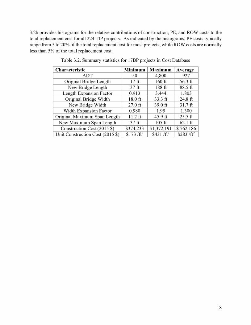
18

3.2b provides histograms for the relative contributions of construction, PE, and ROW costs to the total replacement cost for all 224 TIP projects. As indicated by the histograms, PE costs typically range from 5 to 20% of the total replacement cost for most projects, while ROW costs are normally less than 5% of the total replacement cost.

Table 3.2. Summary statistics for 17BP projects in Cost Database

Characteristic Minimum Maximum Average ADT 50 4,800 927

Original Bridge Length 17 ft 160 ft 56.3 ft New Bridge Length 37 ft 188 ft 88.5 ft

Length Expansion Factor 0.913 3.444 1.803 Original Bridge Width 18.0 ft 33.3 ft 24.8 ft

New Bridge Width 27.0 ft 39.0 ft 31.7 ft Width Expansion Factor 0.980 1.95 1.300

Original Maximum Span Length 11.2 ft 45.9 ft 25.5 ft New Maximum Span Length 37 ft 105 ft 62.1 ft Construction Cost (2015 $) $374,233 $1,372,191 $ 762,186

Unit Construction Cost (2015 $) $173 /ft2 $431 /ft2 $283 /ft2

19

a)

b)

Figure 3.2. Relative contributions of component costs to total costs for 224 TIP bridge projects in Cost Database: a) average; b) histograms for component costs

Figure 3.3 provides histograms for the component costs normalized by the deck area of the replaced and replacement structures to express such component costs as unit costs. The distributions of unit costs are not normally distributed and are typically skewed toward the lower end of the range for each unit component cost. The unit costs computed relative to the deck area of the replaced bridge vary significantly more than the unit costs computed relative to the deck area of the replacement bridge. This reflects the significant variation the change in deck area resulting from lengthening and widening of bridges during replacement. Summary statistics for the unit construction cost by project and route type, computed using the deck area of the replacement structure, are presented in Table 3.3. As reflected in this table, the unit construction cost for bridges on primary and interstate routes are typically higher than for bridges on secondary routes. Also, the average unit construction costs for the 17BP projects contained in the Cost Database are typically higher than the average unit construction costs for TIP projects on similar route types. Table 3.4 presents summary statistics for the unit total replacement costs, which are computed only for the TIP projects for which all component costs were provided. As with unit construction costs, the unit total replacement costs for bridges on primary routes were observed to be typically higher than the unit total replacement costs for bridges on secondary routes.

20

a)

b)

Figure 3.3. Unit component costs for bridge projects in Cost Database: a) calculated using deck area of replaced structure; b) calculated using deck area of replacement structure (PE and ROW

costs available only for TIP projects)

Table 3.3. Summary statistics for unit construction cost ($/ft2) by route classification using deck area of replacement bridge

# Minimum Maximum Mean Median Standard Deviation

TIP Projects Primary 22 $158 $446 $255 $247 $59 Secondary 201 $115 $369 $211 $202 $45

17BP Projects Primary 12 $246 $393 $302 $281 $53 Secondary 67 $173 $431 $279 $272 $58

All Projects Primary 34 $158 $446 $272 $254 $61 Secondary 268 $115 $430 $228 $215 $57 Interstate 3 $195 $364 $276 $268

21

Table 3.4. Summary statistics for unit total cost ($/ft2) by route classification for TIP projects using deck area of replacement bridge

# Minimum Maximum Mean Median Standard Deviation

Primary 22 $182 $492 $302 $295 $67 Secondary 201 $158 $436 $251 $243 $55 Interstate 1 $246

3.1.2. Development of Database for Predicting Changes in Bridge Characteristics

To facilitate the development of predictive models to forecast changes in bridge characteristics during replacements, a secondary database was developed using data from the Performance Master to obtain information on bridge replacements. The reason for developing this secondary database was to expand the information on changes in bridge characteristics occurring during bridge replacements beyond the limited number of projects contained in the Cost Database. Performance Master data from 2006 was used to extract records for bridges replaced during the ten year period between 2007 and 2016. Records from the 2006 Performance Master were linked to the 2017 Network Master using the structure number, which is unique to each bridge and common to both databases. The Year Built item in the Network Master was used to identify all potential replacement projects from this time frame, while location and structure type information in the Performance Master was used to confirm that each project was a bridge-to-bridge replacement project. Since the objective of the statistical models developed from this dataset is to forecast changes in bridge characteristics during replacement projects for representative structures undergoing typical replacement, instances of bridge replacements that were deemed to be atypical were filtered from the dataset. Examples of atypical replacement projects are bridges with more than nine spans, moveable bridges, and replacement projects that involve very large changes in length or width relative to the original structure. As with the generation of the Cost Database, the NBI files submitted by NCDOT to the FHWA were used to source the maximum span length for both the replaced and replacement bridges since this item is not recorded in the Performance Master. The maximum span length was extracted from Item 48 – Length of Maximum Span in the record for each structure using the NBI data corresponding to the same year of the Performance Master data that this item was linked to.

The assembled database is herein referred to as the Characteristics Database, since it is used to develop statistical models for forecasting the changes in bridge characteristics occurring during bridge replacement, such as the changes in structure length, width, and length of maximum span. The Characteristics Database includes a total of 1,506 bridge replacement projects occurring between 2007 and 2016. This set consists of 1,201 bridges on secondary routes, 286 bridges on primary routes, and 19 bridges on interstate routes. Table 3.5 provides a further breakdown of the project count by functional classification and system classification of the route carried by the bridge. Table 3.6 provides summary statistics for the geometric characteristics for the bridges contained in the Characteristics Database. As expected, the range of the geometric characteristics

22

for the projects contained in the Characteristics Database encompass those for the projects contained within the Cost Database. This ensures that the application of statistical models generated from the Characteristic Database to bridges contained in the Cost Database does not involve extrapolation of the models outside of the range of the underlying data used to develop the models.

Table 3.5. Breakdown of replacement projects in Characteristics Database by functional classification and system classification of route carried

Primary Secondary Interstate All Routes Local 65 897 5 967 Minor Collector 26 179 3 208 Major Collector 102 83 0 185 Minor Arterial 54 34 1 89 Principal Arterial 39 8 10 57 Total 286 1,201 19 1,506

Table 3.6. Summary statistics for bridge replacement projects in Characteristics Database

Characteristic Minimum Maximum Average ADT 10 90,000 2,477 Original Bridge Length 15 ft 873 ft 78.7 ft New Bridge Length 16 ft 873 ft 112.1 ft Length Expansion Factor 0.459 10.912 1.648 Original Bridge Width 11.6 ft 99.9 ft 24.4 ft New Bridge Width 12 214.9 ft 35.2 ft Width Expansion Factor 0.466 5.970 1.462 Original Maximum Span 7.9 ft 180.1 ft 31.0 ft New Maximum Span 14.1 ft 252.0 ft 64.1 ft

3.2 Review and Evaluation of Current Cost Estimation Strategies Currently, NCDOT computes conceptual replacement cost estimates for all bridges in the state inventory using a simple unit cost model implemented in the BMS. These unit costs are multiplied by the deck area of the current (replaced) bridge to arrive at an estimate of the total replacement cost. In the simple unit cost model currently used by NCDOT, the unit cost is determined only by the classification of the route carried by the structure. Unit costs of $704/ft2 are used for bridges on interstate routes, $664/ft2 are used for bridges on primary routes, and $529/ft2 are used for bridges on secondary routes.

Since the unit costs currently used in the BMS are associated with the current deck area of each bridge in the inventory, summary statistics for unit construction costs and unit total replacement costs were generated for the bridges in the Cost Database using the deck area of the replaced structures. These summary statistics are presented in Table 3.7 and 3.8, respectively. In contrast to the unit costs computed with the deck area of the replacement structures, the range for

23

the unit costs computed with the deck area of the replaced structures is very wide. While the average unit construction and average unit total replacement costs do exhibit typically larger values for bridges carrying primary routes compared to secondary routes, the large standard deviations observed across the datasets suggest that system classification of the route alone does not correlate strongly with the unit construction cost or the unit total replacement cost. The mean unit total replacement cost for the 22 TIP bridges on primary routes in the Cost Database does fall within $1/ft2 of the unit cost currently being used in the NCDOT BMS, but this alone does not support the use of the current cost estimation strategy given the large spread and standard deviation of the unit total replacement costs observed in the Cost Database.

Table 3.7. Summary statistics for unit construction cost ($/ft2) by route classification using deck area of replaced bridge

# Minimum Maximum Mean Median Standard Deviation

TIP Projects Primary 22 $292 $1,297 $561 $514 $241 Secondary 201 $163 $1,965 $530 $496 $244

17BP Projects Primary 12 $371 $2,057 $865 $614 $522 Secondary 67 $266 $1,586 $651 $600 $291

All Projects Primary 34 $292 $2,057 $669 $535 $387 Secondary 268 $163 $1,965 $561 $520 $261 Interstate 3 $325 $739 $518 $491

Table 3.8. Summary statistics for unit total cost ($/ft2) by route classification for TIP projects using deck area of replaced bridge

# Minimum Maximum Mean Median Standard Deviation

Primary 22 $319 $1,432 $663 $600 $266 Secondary 201 $228 $2,111 $635 $583 $298 Interstate 1 $618

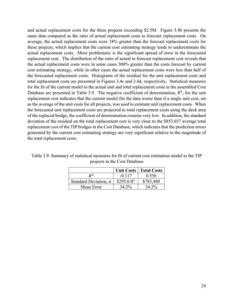
The current cost estimating strategy was used to forecast the total replacement costs for the 224 TIP projects for which total replacement costs were available in the Cost Database. Figure 3.4 compares the actual replacement cost to the replacement cost forecast in the BMS for these projects. In Figure 3.4a, a 1:1 reference line is provided to aid in the comparison. Since the majority of replacement projects in the database have a total replacement cost of less than $2.5M, most of the points are concentrated near the origin of the axis. While the forecasted replacement costs generally correlate with the actual replacement costs, there is a fair amount of scatter in the region where most projects are concentrated and very significant differences between the forecast

24

and actual replacement costs for the three projects exceeding $2.5M. Figure 3.4b presents the same data computed as the ratio of actual replacement costs to forecast replacement costs. On average, the actual replacement costs were 18% greater than the forecast replacement costs for these projects, which implies that the current cost estimating strategy tends to underestimate the actual replacement costs. More problematic is the significant spread of error in the forecasted replacement cost. The distribution of the ratio of actual to forecast replacement cost reveals that the actual replacement costs were in some cases 300% greater than the costs forecast by current cost estimating strategy, while in other cases the actual replacement costs were less than half of the forecasted replacement costs. Histograms of the residual for the unit replacement costs and total replacement costs are presented in Figures 3.4c and 3.4d, respectively. Statistical measures for the fit of the current model to the actual unit and total replacement costs in the assembled Cost Database are presented in Table 3.9. The negative coefficient of determination, , for the unit replacement cost indicates that the current model fits the data worse than if a single unit cost, set as the average of the unit costs for all projects, was used to estimate unit replacement costs. When the forecasted unit replacement costs are projected to total replacement costs using the deck area of the replaced bridge, the coefficient of determination remains very low. In addition, the standard deviation of the residual on the total replacement cost is very close to the $853,037 average total replacement cost of the TIP bridges in the Cost Database, which indicates that the prediction errors generated by the current cost estimating strategy are very significant relative to the magnitude of the total replacement costs.

Table 3.9. Summary of statistical measures for fit of current cost estimation model to the TIP projects in the Cost Database

Unit Costs Total Costs -0.117 0.556

Standard Deviation, $295.6/ft2 $783,480 Mean Error 34.2% 34.2%

25

a) b)

c) d)

Figure 3.4. Comparison between actual replacement cost and replacement cost forecasted by the BMS for TIP projects using deck area of replaced structure: a) cost comparison, b) histogram of

actual costs relative to estimated costs, c) histogram of residuals for unit replacement cost, d) histogram of residuals for total replacement cost

3.2.2 Conceptual Cost Estimates for High Value Bridges

As an alternative to the unit costs used in the BMS, NCDOT forecasts conceptual costs for high value bridges using a dedicated spreadsheet. As of the time that this spreadsheet was shared with the research team, this spreadsheet contained conceptual cost estimates for 205 bridges. This spreadsheet generally does not track historical costs, but rather is based on engineering judgment and is used for planning purposes. In several instances, the costs have been updated to reflect costs

26

sourced from bid tabs or HiCAMS to update the estimates in the spreadsheet to the actual values to provide feedback to the future development of this high value bridge replacement cost estimating tool. Figure 3.5 provides a schematic of the general approach used by NCDOT to generate conceptual cost estimates for high value bridges. The construction cost is developed as the sum of estimated bridge, roadway, and demolition costs. Estimated bridge and demolition costs are based on unit cost estimates, with the deck area of the replacement structure being used to forecast the bridge cost and the deck area of the replaced structure being used to forecast the demolition costs. The use of the deck area of the replacement structure is in contrast to the strategy currently used in the BMS that uses only the deck area of the existing structure. The spreadsheet does not contain a formula for estimating the span length and deck width of the replacement bridge, but these values appear to be entered manually at the discretion of the engineer. PE, ROW and utility costs, and construction engineering and inspection (CEI) costs are then forecast as a function of the estimated construction cost.

Figure 3.5. Conceptual cost estimation approach used in high value bridges spreadsheet

The formulas currently used for estimating the total replacement cost of high value bridges were identified by reviewing the formulas coded into the spreadsheet provided to the research team. From this review, it was determined that the components of the SMU Replacement Cost Estimate are calculated as follows:

∗

(3.1)

27

$66.7 ∗ $88.9 ∗ $100 ∗ $111.1 ∗ $133.3 ∗ $267 ∗ $555.6 ∗

(3.2)

$20 ∗

(3.3)

(3.4)

0.15 ∗ ∶ $4$0.4 0.1 ∗ ∶ $20min $0.1 0.08 ∗ , $20 ∶ $20

(3.5)

$3 ∶ $300.05 ∗ ∶ $30

(3.6)

0.1 ∗

(3.7)

(3.8)

As indicated by the formulas, the construction cost is directly calculated using a unit bridge cost, future deck width, and existing deck area. The unit bridge cost utilized in the spreadsheet varies from $110/ft2 to $1435/ft2. However, only 7 of the bridges in the list use a unit bridge cost greater than $350/ft2 and all of these instances are moveable bridges (bascule, lift truss, or swing). For the non-moveable bridges, the average unit bridge costs used is $193/ft2 with a standard deviation of $38/ft2. Approximately 55% of the non-moveable bridges in the spreadsheet have bridge costs estimated using a $175/ft2. unit bridge cost. The roadway cost most commonly used in the spreadsheet is $66.7k/ft of future width, although this unit cost varies significantly across the set of high-value bridges. The research team was unable to identify a correlation between

28

bridge characteristics and the unit roadway cost used in the spreadsheet, and it was assumed that the unit roadway cost was identified for each bridge based on experience and engineering judgment provided by NCDOT personnel.

For high value bridges, the NCDOT conceptual cost estimates for PE cost and ROW and Utility Costs are computed as a function of the construction costs. In both cases, these costs are assumed to scale with the magnitude of the construction costs up to a fixed maximum cost ($20M for PE cost and $3M for ROW and Utility Costs). Interestingly, when the piecewise linear functions currently being used to estimate PE costs are plotted (Figure 3.6), a discontinuity is revealed in the cost prediction model. Likewise, a discontinuity was discovered in the piecewise linear model for ROW and Utility Costs (Figure 3.7). The reason for these discontinuities is not known, although the research team suspects that they reflect an error in the formulation of the piecewise linear functions. Significant discontinuities within cost prediction models should be avoided unless strongly justified since they lead to large differences in estimated total project costs between bridges that otherwise have very small differences in construction costs. For example, due to the discontinuity in the PE cost model, the current estimating spreadsheet would predict that a bridge with a construction cost one dollar under $20M would have a PE cost of $2.4M, while a bridge with a construction cost one dollar over $20M would have a PE cost of only $1.7M. Likewise, the current estimating spreadsheet predicts that a bridge with a construction cost one dollar under $30M would have a ROW and Utility Cost of $1.5M, while a bridge with a construction cost one dollar over $30M would have a ROW and Utility Cost of $3M.

Figure 3.6. Discontinuity in piecewise linear function currently being used to forecast PE costs for high value bridges

29

Figure 3.7. Discontinuity in piecewise linear function currently being used to forecast ROW and Utility Costs for high value bridges

The construction costs for the high value bridges in this spreadsheet range from $10.4M to $367M. These construction costs are orders of magnitude greater than most of the bridges in the Cost Database assembled for this research effort. Only one bridge within the Cost Database had a construction cost greater than the lowest cost bridge in the high value bridges list. Consequently, the available cost data from the assembled Cost Database cannot be used to assess or validate the forecasting equations currently being used by NCDOT for high value bridges. However, comparisons for simple statistics of component costs were developed to provide some insight into the plausibility of the models used.

Within the Cost Database of 224 non-high value TIP bridge replacements, PE costs were on average 16.8% of the construction cost, but tended to decrease as a percentage with increases in construction cost. The high value bridge cost estimation model projects PE costs to be 15% of construction costs for bridges with construction costs less than $4M, which seems reasonable given the cost data for the projects in the Cost Database. The moderate decrease in relative PE costs to only 10% of construction costs over $20M cannot be assessed based on the available data, but is generally supported by the observed trend of reduced relative PE costs with increased construction cost. ROW costs were on average 2.5% of the construction costs, which is half of the relative fraction of construction costs predicted by the high value bridge cost estimation model. This suggests that the high value bridge conceptual cost estimates may be overly-conservative in their forecasts of ROW and utility costs. However, the lack of sufficient data for bridges with construction costs in the same range as the bridges in the high value bridge spreadsheet precludes any basis for assessing the validity of the current high value bridge cost estimation models.

30

3.3 Development of Improved Cost Estimation Strategies for the BMS

3.3.1. Predictor Variables

Potential predictor variables for the statistical regressions available in the assembled databases included geometric characteristics of the replaced and replacement structures, functional and geographic characteristics, usage statistics and system classifications, appraisals, and design details. Table 3.10 presents a summary overview of all of the predictor variables explored for use in the development of the improve cost estimation strategies for the BMS. This table lists the predictor variable by a shorthand descriptor, a brief description of the predictor variable, the type of predictor variable, and the type of cost forecasting model where the predictor variable was made available for regression. Many of the shorthand descriptors used for each predictor variable were adopted from the Abed-al-Rahim and Johnston (1995) study to maintain consistency and facilitate ease of model comparison between this prior NCDOT sponsored research effort and the current one. For the Type A forecasting models, only information about the replaced bridge is used to construct regression models capable of forecasting replacement costs directly from the characteristics of the replaced bridge. For the Type B forecasting models, the costs are computed using characteristics of the replacement bridge, which must be predicted from the characteristics of the replaced bridge through intermediate prediction models. Most of the variables used are defined in the Recording and Coding Guide for the Structure Inventory and Appraisal of the Nation’s Bridges (FHWA 1995), although some variables are not found in the NBI. Additionally, grouping was applied to some of the categorical variables due to limited diversity in the available data. Deviations from the standard NBI descriptions are detailed in the following paragraphs. Further details on the assembly of the bridge replacement databases and predictor variables can be found in a Master of Science thesis stemming from this research (Phillips, 2017).

31

Table 3.10. Summary of predictor variables used in statistical regressions

Predictor Variable Description Type Models OBLEN Span length of replaced bridge Continuous A OBWID Deck width of replaced bridge Continuous A MAXSPAN1 Maximum span in replaced bridge Continuous A NBLEN Span length of replacement bridge Continuous B NBWID Deck width of replacement bridge Continuous B MAXSPAN2 Maximum span in replacement bridge Continuous B WATERDEPTH Depth of water under bridge Continuous A,B BRIDGEAGE Age of replaced bridge Continuous A,B CTB Crown-to-bed height of replaced bridge Continuous A,B APPWID Approach roadway width of replaced

bridge Continuous A,B

LEF Length Expansion Factor Continuous B WEF Width Expansion Factor Continuous B ADT ADT for replaced bridge Continuous A,B REGION Geographic region Categorical A,B DIVISION Highway division Categorical A,B FUNCTCLASS Functional classification of route Categorical A,B SUPERSTRMAT Superstructure Material Type Categorical A,B SUPERSTRTYPE Superstructure Design Type Categorical A,B SUBSTRMAT Substructure Material Type Categorical A,B DECKMAT Deck Material Type Categorical A,B MULTISPAN Number of Spans Categorical A,B DECKGEOMAPP Deck Geometry Appraisal Adequacy Binary A,B ROADWAYALIGNAPP Roadway Alignment Appraisal

Adequacy Binary A,B

UNDERAPP Waterway or Underclearance Adequacy Binary A,B SECONDARYBRIDGESYS Route type (Secondary or Not

Secondary) Binary A,B

PROJECTTYPE Project type (17BP or TIP) Binary A,B

Continuous variables included in the statistical regressions included the structure length, deck width, maximum span length, depth of water under the bridge, bridge age, crown-to-bed height, approach roadway width, length expansion factor, width expansion factor, and ADT. In contrast to the NBI records, all continuous variables related to length use units of feet to maintain consistency with the units used within the BMS.

WATERDEPTH: All 305 bridges in the Cost Database cross over water, which could range from a shallow creek to a deep river or bay inlet. The depth of the water under the bridge was considered as having a possible influence on costs due to the role that flood plains and scour have on bridge designs. An existing bridge that crosses a river may require height and length increase, including additional ROW purchases, during replacement to comply with modern design standards. Additionally, bridges with piers in deep water may require

32

greater demolition and construction costs as a result of special equipment and methods that may need to be employed.

BRIDGE AGE: The bridge age was calculated as the difference between the recorded year that the replacement bridge was built and the original year that the replaced bridge was built. This variable was considered as a potential predictor variable because an older bridge may require additional length expansion to accommodate modern scour design requirements, additional width expansion to accommodate increased traffic, and more extensive environmental protection measures during demolition or site improvements during replacement than associated with bridge replacements performed on bridges built more recently.

CTB: The “crown” of a bridge is defined as the apex of its arch (Kassler, 1949). The crown-to-bed height is not recorded in the NBI, but is an item recorded in the BMS. For the purposes of this work, it was inferred that the measurement from the bed of the feature that the bridge is crossing to the top of the bridge crown represents the maximum height of the bridge structure. Bridges with larger crown-to-bed heights are expected to have increased replacement costs.

APPWID: The approach roadway width includes the roadway width plus any usable shoulder areas on either side. The approach roadway width used in the statistical regression is the recorded value sourced from the Performance Master database for the replaced bridge.

LEF: The length expansion factor is the ratio of the span length for the replacement bridge to the span length of the replaced bridge.

WEF: The width expansion factor is the ratio of the deck width for the replacement bridge to the deck width of the replaced bridge.

ADT: This continuous predictor variable is the average daily traffic estimate for the route carried by the bridge at the time of replacement.

Categorical variables included in the statistical regressions included geographic region and highway division, functional classification of the route carried by the structure, the superstructure material and design type, the substructure and deck material types, and the number of spans in the bridge. Abed-al-Rahim and Johnston (1995) did not use such categorical variables, but explored the possibility of creating separate models for different bridge types. However, their final prediction models utilized only continuous variables.

REGION: The region is a classification of the geographic region where the bridge is located, which is recorded in the BMS. There are three geographic regions used in the state: Coastal (1), Piedmont (2), and Mountain (3). The Cost Database included 31 coastal, 152 Piedmont, and 122 mountain projects. Figure 3.8 presents a map of the location of each individual bridge replacement project in the Cost Database.

DIVISION: This categorical variable indicates the highway division for the location of the bridge replacement project. Bridge replacement projects from all 14 highway divisions were included in the Cost Database.

33

FUNCTCLASS: The Cost Database contained bridges across six functional classifications: local (224 bridges), minor collector (47 bridges), major collector (29 bridges), minor arterial (1 bridge), principal arterial – interstate (1 bridge), and principal arterial – other (3 bridges). Due to the limited number of bridge replacements on principal and minor arterials in the Cost Database, the two principal arterial, the minor arterial, and the major collector functional classifications were combined to form one category.

SUPERSTRMAT: This categorical variable designates the predominant material of the superstructure for the bridge being replaced. The Cost Database included 49 concrete superstructures, 188 steel superstructures, and 68 timber superstructures.

SUPERSTRTYPE: This categorical variable designates the superstructure design type for the bridge being replaced. The Cost Database included 23 channel beam, 21 girder and floorbeam system, 236 stringer/multi-beam or girder, and 25 other superstructure types.

SUBSTRMAT: This categorical variable designates the predominant material of the substructure for the bridge being replaced. The Cost Database included 42 concrete substructures, 152 timber substructures, and 111 substructures of other material.

DECKMAT: This categorical variable designates the predominant material of the deck for the bridge being replaced. The Cost Database included 122 concrete decks, 25 steel decks, and 158 timber decks.

MULTISPAN: This categorical variable designated the number of spans in the bridge being replaced. The Cost Database included 99 single span bridges, 72 two span bridges, 78 three span bridges, 30 four span bridges, 23 five span bridges, 2 eight span bridges, and 1 nine span bridge. A few instances of bridges with more than nine spans were considered atypical and were removed from the Cost Database to avoid potential skew in the regression models caused by their inclusion. Due to the limited number of bridges with more than five spans, all bridges with more than five spans were condensed into the same category as bridges with five spans.

DECKGEOMAPP: Adequacy of the deck geometry is evaluated through the clear deck width and minimum vertical clearance over the bridge, with the lower of the two conditions dictating the deck geometry appraisal (FHWA 1995). The deck geometry appraisals were binned into a binary classification in order to create larger groups for regression and to reduce the complexity of the prediction models. The binary classification was developed by classifying all bridges with a deck geometry rating of 4 or greater as “acceptable” and with a deck geometry rating of 3 or less as “unacceptable.” This threshold was established by the definitions for this appraisal, as corrective action is indicated for bridges receiving an appraisal of 3 or less. The Cost Database included 163 bridges with deck geometries classified as acceptable and 142 bridges with deck geometries classified as unacceptable.

ROADWAYALIGNAPP: The roadway alignment for a bridge is appraised by the change in speed required due to the alignment of the approach roadway relative to the bridge deck. The Recording and Coding Guide for the Structure Inventory and Appraisal of the Nation’s Bridges specifies a rating of 6 for structures requiring only a minor reduction in speed and a rating of 8 for structures requiring no reduction in speed. Binary classification was developed for this variable by classifying all bridges with an appraisal of 6 or greater as “acceptable” and all bridges with an appraisal of less than 6 as “unacceptable.” The

34

rationale for including this appraisal as a potential predictor variable was that poor approach roadway alignment may necessitate ROW purchases, wider bridge decks, or expensive modifications to the approach roadway or structure alignment to correct the roadway alignment issue. The Cost Database included 294 bridges with roadway alignment classified as acceptable and 11 bridges with roadway alignment classified as unacceptable.

UNDERAPP: This binary variable indicates the adequacy of the waterway if the bridge is over a waterway or underclearance below the bridge if it is over another route. As with the other appraisals, this variable was developed as a binary variable. The Cost Database included 298 bridges with acceptable underclearance and 7 bridges with an unacceptable underclearance.

SECONDARYBRIDGESYS: This binary variable indicates the classification of the highway system for the route carried by the replaced structure. Since there were only 3 interstate bridges in the Cost Database, the interstate bridges were combined with bridges on primary routes to develop a binary classification system. The Cost Database included 268 bridges on secondary routes and 37 bridges that are not on secondary routes.

PROJECTTYPE: This last predictor variable is a binary classification of whether the bridge replacement project was funded under the 17BP or TIP program.

Figure 3.8. Locations of TIP and 17BP bridge replacement projects in Cost Database

3.3.2. Summary of Cross Validation and Statistical Regression Techniques

All regression models developed from this research used 5-fold cross validation to minimize over-fitting of the models to the underlying data. As detailed in the literature review, k-fold cross validation is an approach where the dataset is randomly divided into training sets on which the statistical models are constructed and test sets where the prediction errors developed by the statistical models are assessed. A 5-fold cross validation involves developing five regression models on training sets each comprising 80% of the database, where the test sets each comprise the remaining 20% of the database. The mean square error calculated when applying regression models developed from training sets to the test sets was used as the measure for the cross validation loss. This cross validation loss measure provides a means for optimizing the complexity of the

35

regression model in a way that maximizes the fit to the data while maintaining the strongest predictive capabilities of the model when applied to future data. This is illustrated in Figure 3.9. As the complexity of the model increases by either adding more branches to a decision tree or more predictor variable to a generalized linear regression model, the predictive capabilities of the model will improve as the fit to the underlying data improves. However, with further increasing complexity, the regression model will begin to over-fit to the underlying data in the training set and result in increased prediction errors when applied to data in test or future sets, which are not used to develop the regression model. The optimal model complexity is the point at which the cross validation loss is minimized. The complexity of the model is quantified through hyperparameters specific to the type of regression model. For example, for linear regression models, the number of terms in the model might be a hyperparameter to be optimized to arrive at the optimal complexity.

Figure 3.9. Illustration of tradeoff between complexity of regression model and cross validation loss

Generalized linear regression was used to produce regression models for cost components and all changes in bridge characteristics needed for computing cost components using the regression models. Generalized linear regression is an extension of ordinary linear regression that allows for additional relations between the model and the response variable than the identity function. These relations are call link functions and include log transformation, logit and probit functions, reciprocal, power laws, and other mathematical relationships. In this research, the identity link function and log link function were explored as options for each regression model. In addition, generalized linear regression is not limited to response variables with normal distributions (Agresti, 2015). Inverse Gaussian distributions were specified for all of the generalized linear regressions performed in this study. Stepwise forward selection of predictor variables was performed to construct each regression model, with the Akaike Information Criterion (AIC) used to identify the selection of the predictor variable to add to each model during the stepwise construction. The AIC minimizes with the likelihood function of the model and is penalized by the number of parameters included in the model to balance the tradeoff between goodness of fit

36

and model complexity (Pardoe, 2012). The stepwise forward process begins with the constant or intercept term and then progressively adds predictor variables to model until the specific maximum number of steps is reached. Linear terms (ex. NBLEN) as well as quadratic terms (ex. NBLEN2) and interaction terms (ex. NBLEN*NBWID or NBLEN*CTB2) were permitted to be selected by the stepwise regression process. To arrive at the optimal model complexity, Bayesian optimization was used to minimize the cross validation loss using the number of steps in the stepwise regression and form of the link function (either identity or log) as hyperparameters. Through this approach, the Bayesian optimization provides an estimate for the ideal number of terms in the generalized linear regression model and the link function that results in the model with the best cross validated predictive capabilities.

In addition to generalized linear regression models, binary decision trees were also developed through regression for each of the cost components. Bayesian optimization was used to arrive at the optimal tree structure for each model that minimizes the 5-fold cross validation loss. The minimum leaf size was used as the optimized hyperparameter for construction of each of the decision trees. This minimum leaf size is the smallest number of observations contained within any leaf, or node, of the decision tree. As the leaf size decreases with model complexity, the data is able to improve the fit to the underlying data, but leaf sizes too small result in overfitting of the model to the data. Use of the minimum leaf size as a hyperparameter in the Bayesian optimization results in a model that appropriately balances the model complexity with the expected predictive capabilities when applied to future data. To ensure averaging of a sufficient number of projects within each leaf, the minimum permissible leaf size for any of the developed models was constrained to 12. This minimum permissible leaf size ensures that each estimated unit cost in the decision trees results from the averaging of no less than 5% of the bridge replacement projects contained in the Cost Database. Lastly, in order to arrive at compact models, pruning of the developed binary decision trees was performed to remove any leaves that did not appreciably affect the goodness of fit, as measured by the coefficient of determination.

3.3.3. Construction Cost

For the development of the improved cost estimation models, regressions were performed on the total construction costs for each structure as well as the unit construction costs. By producing regression models for both the total and unit normalized costs, model goodness of fit statistics could be used to evaluate whether projecting total construction costs results in improved predictive performance compared to projecting the unit construction costs and then multiplying those projected unit costs by the deck area to arrive at the total construction costs. Since construction costs were available for both the 17BP and TIP projects, all 305 bridge replacement projects in the Cost Database were included in the regressions.

Improved cross validated goodness of fit was observed for construction costs when the regression models were used to forecast the unit construction costs rather than the total construction costs. Similarly, the goodness of fit for models developed on unit PE and unit ROW costs were improved relative to those developed on total PE and total ROW costs. Consequently, the statistical regressions presented in this study forecast the unit component costs rather than the total component costs. To arrive at estimates of the total component costs for the Type A models,

37

the unit component costs are multiplied by the deck area of the replaced structure (the old bridge). To arrive at estimates of the total component costs for the Type B models, the unit component costs are multiplied by the deck area of the replacement structure (the new bridge). Histograms of the unit construction costs calculated using the deck area of the replaced bridge and the deck area of the replacement bridge were previously presented in Figure 3.3. The minimum, maximum, and average unit construction costs computed using the deck area of the replaced bridge were $163/ft2, $2057/ft2, and $572/ft2, respectively. The minimum, maximum, and average unit construction costs computed using the deck area of the replacement bridge were $115/ft2, $446/ft2, and 233/ft2, respectively.

The optimal cross validated Type A model developed for unit construction costs using generalized linear regression uses the log link function and takes the formula:

$

3828.39 ∗ ∗ ∗ ∗ ∗ ∗

1.0 0.6562 20.5477 30.4325 40.4210 5

1.0 1.2767 17

0.0183; 0.006; 1.1992 10 ;

0.0865; 1.5107 10 ; 8.8821 10

(3.9)

Interpretation of the significance of the predictor variable and regression coefficients within Type A models cannot be directly performed in many cases, since these models are internally forecasting both the unit construction costs and the projected change in deck area. For example, in this model, multiple span bridges are forecast to have reduced unit construction costs compared to single span bridges with increased reductions in unit construction costs for each additional span. This effect of number of spans on the unit construction cost may be a reflection of the changes in structure length rather than a correlation between number of spans and actual unit construction cost. Single span bridges are typically shorter than multiple span bridges and shorter span bridges generally experience greater relative length expansion during replacement than longer span bridges, so this effect of number of spans contained within the model may simply be compensating for the expected length expansion. Other predictor variables, such as project type and bridge age at the time of replacement, are static variables and can be directly interpreted. This model projects a 28% increase in unit construction cost for 17BP projects relative to TIP projects and increased unit construction cost with an increase in the age of the bridge being replaced.

38

The Type A binary decision tree developed for unit construction cost is presented in Figure 3.10. The minimum leaf size for this model is 12, which means that each of the unit cost values presented in the tree were arrived at by averaging no less than 12 replacement projects. The most significant predictor variable within this model is the original bridge length, with unit construction costs consistently reduced with increased length of the original bridge being replaced. The second most significant predictor variable within this model is the original bridge width, with unit construction costs reduced for bridges with larger original deck widths.

Figure 3.10. Decision tree for unit construction costs applied to replaced bridge deck area

39

The optimal cross validated Type B model developed for unit construction costs using generalized linear regression takes the formula:

$

378.87 . ∗ . ∗ . ∗

1.0 0.9987 21.0431 30.9814 41.0536 5

1.0 1.1260 1.1260

1.0 1.2819 17

(3.10)

As with the Type A model developed for unit construction costs, the log link function was found to produce the lowest cross validated mean squared error. The Type B model predicts that 17BP projects will have a 28% increase in unit construction costs compared to TIP projects and that bridge replacements on primary or interstate routes are 12.6% more costly on a unit construction basis than bridge replacements on secondary routes. In contrast to the Type A model, the number of spans only has a nominal effect on the unit construction costs in this Type B model, which suggests that the effect observed in the Type A model is a mechanism for indirectly accounting for the change in deck area in the Type A model. The most significant predictor variable in the Type B regression model is the length of the replacement structure. Figure 3.11 presents an illustration of the effect of the span length on the forecast unit construction cost if the replacement project occurs on a secondary route with low ADT through TIP funding. As illustrated in the figure, the predicted unit construction cost sharply decreases with an increase in structure length until approximately 200ft, where the unit construction cost is predicted to increase. This figure also raises an important practical consideration related to the implementation of these models, as this nonlinear function is fit to cost data from a database consisting of predominantly short span bridges. The largest structure length of the replacement bridges used in the regression analysis is 331ft, which corresponds to the axis limit of Figure 3.11. If the Type B unit construction cost model is applied to predict unit construction costs for replacement bridges with longer structure lengths, then this would be an extrapolation beyond the region of the model and could potentially result in extremely large estimates of unit construction costs. This is particularly an issue due to the nonlinear nature of the regression equation and the presence of the log transformation.

40

Figure 3.11. Predicted effect of structure length on unit construction cost in Type B model for a TIP bridge replacement on a secondary route with low ADT

The Type B decision tree developed for unit construction costs is presented in Figure 3.12. The minimum leaf size for this model is 17. Consistent with the generalized linear regression model, 17BP project are identified as having moderately higher unit construction costs than TIP projects and the most significant predictor variable identified by the decision tree is the length of the replacement structure. However, since the decision tree is limited to a small number of binary splits, this model only predicts a consistent decrease in unit construction costs with an increase in the length of the replacement structure. This allows the decision tree to be extrapolated to replacement projects for bridges with structure lengths exceeding the 331ft maximum length observed in the Cost Database without the potential for extremely large unit construction costs being incorrectly forecast. However, it should be cautioned that this would still be an extrapolation of the model, which will likely fail to capture potential further decreases in unit construction costs for long span bridges resulting from economy of scale. An important consideration for the future improvement of the developed cost estimation models is the cataloging of bridge replacement costs for high value bridges and other structures with atypical characteristics outside of the bounds captured by the bridges in the Cost Database used in this study.

41

Figure 3.12. Decision tree for unit construction costs applied to replacement bridge deck area

Summary statistics for the all of the cross validated regression models developed for unit construction costs are presented in Table 3.11. The coefficient of determination, , and standard deviation of the prediction errors, , are provided for application of each model to the underlying unit construction cost data as well as projected to the total construction costs for each of the 305 bridge replacement projects. Appendix B provides cost comparison plots and histograms for all of the unit construction cost models. Note that the unit costs for the Type A models are calculated using the deck area of the replaced bridge, while the unit costs for the Type B models are calculated using the deck area of the replacement bridge, so the statistical measures for the unit costs should not be compared across these two types of models. However, the statistical measures for the total costs can be directly compared. For both the Type A and Type B models, the generalized linear regression resulted in a better fit and smaller prediction errors than the binary decision trees. The performance of the two generalized linear regression models was similar, with the Type B model achieving a slightly better fit and lower standard deviation than the Type A model. However, these summary statistics were computed using the actual characteristics of the replacement bridges rather than predicted characteristics of the replacement bridges. In Section 4 of this report, the effects of using statistical regression models to predict the characteristics of the replacement bridges on the replacement costs forecast by the Type B model is evaluated.

42

Table 3.11. Summary statistics for unit construction cost models

Unit Costs Total Costs Predictor Variable Set Regression Model A: Replaced Bridge Decision Tree 0.677 $158.4/ft2 0.660 $531,610 A: Replaced Bridge GLM 0.754 $138.2/ft2 0.976 $140,700 B: Replacement Bridge Decision Tree 0.574 $38.5/ft2 0.825 $381,460 B: Replacement Bridge GLM 0.592 $37.7/ft2 0.983 $120,500

3.3.4. Preliminary Engineering Cost

As summarized in the literature review, an extensive study on PE costs for bridge and roadway projects was recently conducted for NCDOT (Liu, et al. 2011). This work was reviewed in order to explore the potential to leverage this past research within the current effort. However, it was ultimately determined that the model developed in RP2010-10 to predict PE costs for bridge projects would likely not be suitable for implementation as part of the updated bridge replacement conceptual cost estimation models. One reason why the models were found to be unsuitable was that they would require a number of predictor variables that are not readily sourced from the BMS. Specifically, these prior models used the project construction scope, planning document responsible party, and roadway percentage of construction cost, which are not currently defined or forecast in the BMS. Additionally, the models require the ROW cost and construction cost, so they would be dependent of the accuracy of the other component cost estimation models developed for forecasting bridge replacement costs. Another reason why the PE cost estimation models from RP2010-10 were not utilized was that there were significant differences in the PE cost ratios observed in the assembled Cost Database compared to those presented in the prior work. Figure 3.13 presents the histogram for PE cost ratios for bridge projects presented in Hollar et al. (2013) alongside a histogram for PE cost ratios for the TIP bridge replacement projects analyzed in this current study. While both distributions are left-skewed and non-normally distributed, it is apparent that the PE cost ratios for the bridge replacement projects performed between 2012 and 2016 are generally significantly lower than the PE cost ratios for the bridge projects performed between 2001 and 2009 that were analyzed in the prior NCDOT research. The average PE cost ratio observed in the dataset used within the RP2010-10 study was 27.8%, the average PE cost ratio for the 224 TIP projects contained in the developed Cost Database was only 16.8%. The reason for the significant decrease in PE cost ratios between these two time periods is unknown. The RP2010-10 study did not specify the exact nature of the bridge projects, so it is likely that the costs analyzed in the prior research included rehabilitation projects and new bridge construction in addition to bridge replacement projects, so the differences in PE cost ratios may simply be a result of differences in the scope of projects encompassed by each database.

43

a) b)

Figure 3.13. PE cost ratio histograms for bridge projects: a) bridge projects in RP2010-10 (from Hollar, et al. 2013); b) TIP bridge replacement projects in Cost Database

One of the recommendations from the prior research was to analyze preliminary engineering costs in monetary units rather than forecasting the PE costs as a ratio of the construction costs (Hollar, 2013). In the current study, statistical regressions were performed on both the PE cost ratio as well as the unit PE costs and it was determined that improved goodness of fit was achieved when the unit PE cost was the dependent variable. Cross validated generalized linear regression models and binary decision trees were developed for unit preliminary engineering costs using the same approach utilized for the unit construction cost models. However, since preliminary engineering costs were only available for the TIP projects, only a subset of the Cost Database consisting of 224 TIP projects were used to develop the unit preliminary engineering cost models. For these projects, the minimum, maximum, and average unit PE costs computed using the deck area of the replaced bridge were $10.1/ft2, $434/ft2, and $89.5/ft2, respectively. The minimum, maximum, and average unit PE costs computed using the deck area of the replacement bridge were $4.1/ft2, $128.9/ft2, and 35.6/ft2, respectively.

The optimal cross validated Type A model developed for unit PE costs using generalized linear regression uses the identity link function and takes the formula:

$

130.2

0 7.78 256.33 355.11 471.37 5

0 427.57 4

(3.11)

This model uses on the deck geometry rating prior to replacement and the number of spans in the replaced bridge to estimate the replacement cost. Bridges having deck geometry ratings less than

44

4 are forecast to have higher PE costs than bridges with deck geometry ratings not requiring corrective action. This is a plausible correlation, as more preliminary engineering may be required to address width expansion or address issues with vertical clearance over the roadway. With respect to the effect of the number of spans on the unit PE cost, it is not possible to directly associate this predictor variable with PE costs, since it may change during the bridge replacement. As previously noted, the Type A regression models indirectly account for projected changes in deck area since they are based on the unit area of the replaced bridge. Consequently, the reduction in unit PE cost with number of spans reflected in the model may be a reflection of economy of scale, but it is also likely to be the result of the need for the model to indirectly forecast the length and width expansions, which are expected to be greater for shorter, single span bridges, than longer multiple span bridges.

The Type A binary decision tree developed for unit PE cost is presented in Figure 3.14. This decision tree features a minimum leaf size of 38 and uses only the length, width, and deck geometry rating of the replaced bridge to estimate the unit PE cost. In this model, shorter and narrower bridges are associated with higher unit PE costs. For bridges with original span lengths exceeding 41.5ft, the unit PE cost is forecast to be higher if the deck geometry rating is less than 4, requiring corrective action. This correlation between deck geometry rating and unit PE cost was also observed in the Type A generalized linear regression model.

Figure 3.14. Decision tree for unit preliminary engineering costs applied to replaced bridge deck area

45

The optimal cross validated Type B model developed for unit PE costs using generalized linear regression takes the formula:

$

59.68 5.3919 ∗

0 1.92 29.77 39.38 418.89 5

0 10.10 10.10

0 11.14 14.39

(3.12)

As with the Type A generalized linear regression model for PE costs, the identity link function was found to produce the lowest cross validated mean squared error. This model implies a reduction in unit PE costs as the number of spans is increased and an increase in unit PE costs if the bridge replacement occurs on a primary or interstate route instead of a secondary route. Unit PE costs are forecast by the model to be slightly higher for bridges in the Coastal region, with similar unit PE costs for bridges in the Piedmont and Mountain regions. Lastly, the model predicts a decrease in unit PE costs with increased length expansion factor. In contrast to the Type A model, the Type B model does not utilize the deck geometry rating as a predictor variable.

The Type B binary decision tree developed for unit PE costs is presented in Figure 3.15. The minimum leaf size for the developed decision tree is 18. This tree structure is more complex than the Type A decision tree. For replacement bridges with structure lengths less than 82.5 ft, the unit PE cost is a function of the region and the length of the maximum span. Consistent with the Type B generalized linear regression model, this decision tree forecasts higher unit PE costs for bridges in the Coastal region than for those in the Piedmont or Mountains regions. For replacement bridges with structure lengths of 82.5 ft or greater, the unit PE cost is a function of the depth of the waterway under the bridge, the deck geometry rating, and the structure length. Within this branch of the tree, bridges with a deck geometry rating less than 4 are forecast to incur higher unit PE costs than bridges with deck geometry ratings that do not require corrective action. This is consistent with the correlations observed in both of the Type A models for unit PE cost. Interestingly, the unit PE costs are forecast to decrease with increases in the depth of the waterway under the structure.

46

Summary statistics for the all of the cross validated regression models developed for unit PE costs are presented in Table 3.12. The coefficient of determination, , and standard deviation of the prediction errors, , are provided for application of each model to the underlying unit PE cost data as well as projected to the total PE costs for each of the 244 TIP bridge replacement projects. Appendix B provides cost comparison plots and histograms for all of the unit PE cost models. The coefficient of determination for unit PE costs associated with these models are significantly worse than for the models developed for unit construction costs. However, since the PE costs are a significantly smaller fraction of the total replacement cost, the larger prediction errors are not expected to have significant detrimental effect on the estimated total replacement costs. The binary decision tree models achieved a better fit to the unit costs for both the Type A and Type B models. With respect to the total PE costs, the generalized linear regression model achieved a higher coefficient of determination and lower standard deviation of residuals than the decision tree for the Type A models, while the decision tree achieved a higher coefficient of determination and lower standard deviation of residuals than the generalized linear regression model for the Type B models.

Figure 3.15. Decision tree for unit preliminary engineering costs applied to replacement bridge deck area

47

Table 3.12. Summary statistics for unit preliminary engineering cost models

Unit Costs Total Costs Predictor Variable Set Regression Model A: Replaced Bridge Decision Tree 0.363 $49.7 /ft2 0.587 $68,285 A: Replaced Bridge GLM 0.313 $51.6 /ft2 0.710 $57,492 B: Replacement Bridge Decision Tree 0.289 $15.4 /ft2 0.775 $50,718 B: Replacement Bridge GLM 0.200 $16.4 /ft2 0.624 $65,498

3.3.5. Right of Way Cost

Cross validated generalized linear regression models and binary decision trees were developed for unit ROW costs using the same approach utilized for the unit PE cost models. As with PE costs, the ROW costs were not available for the 17BP bridge replacement projects, so the statistical regressions for unit ROW costs were limited to the 224 TIP projects in the Cost Database. For these projects, the minimum, maximum, and average unit ROW costs computed using the deck area of the replaced bridge were $0/ft2, $155/ft2, and $14.8/ft2, respectively. The minimum, maximum, and average unit ROW costs computed using the deck area of the replacement bridge were $0/ft2, $57.5/ft2, and 5.4/ft2, respectively.

A Type A cross-validated generalized linear regression model was developed for unit ROW costs, but the goodness of fit for this model was very poor. Due to the exceptionally poor fit of the model, no equation is presented in this report in order to eliminate the possibility that it is used in any form of implementation. The Type A binary decision tree developed for unit ROW costs is presented in Figure 3.16. The minimum leaf size used to develop this decision tree was 45. This model also achieved a relatively low goodness of fit, but since a model is needed to arrive at ROW costs within the Type A framework, this model was retained since it outperformed the generalized linear regression model. Despite the relatively poor goodness of fit, this model is not expected to detrimentally impact the estimation of total replacement costs through the Type A approach, since ROW costs are such a small percentage of the overall replacement cost. The developed decision tree forecasts higher unit ROW costs for shorter span bridges, with the largest unit ROW costs being assigned to bridges with span lengths less than 51.5 ft and ADT counts greater than 590. For bridges with structure lengths greater than 51.5ft, the estimated unit ROW cost is dependent on the deck geometry appraisal. The unit ROW cost is forecast to be higher for bridges with deck geometry ratings less than 4 than for bridges not requiring corrective action to address deck geometry functional deficiencies.

48

Figure 3.16. Decision tree for unit ROW costs applied to replaced bridge deck area

The cross-validated generalized linear regression model developed for the Type B approach to estimating unit ROW costs utilizes an identity link function and is formulated as:

$

1.56 0.009753 ∗ 5.433 ∗

0 2.53 2.26

(3.13)

The predictor variable with the most influence in this equation is the width expansion factor,

. The correlation between higher width expansion and increased unit ROW costs is

expected, since significant width expansion would most likely be associated with increase ROW acquisitions and utility relocations. The generalized linear regression model also forecasts a mild increase in unit ROW costs with length of the replacement structure, which is also a plausible correlation. Lastly, unit ROW costs are forecast to be slightly higher within the Coastal region than within the Piedmont or Mountain regions. However, as with the Type A generalized linear regression model, the goodness of fit for this Type B generalized linear regression model was poor, so the correlations expressed within this model should be viewed with skepticism.

The binary decision tree developed for prediction of unit ROW costs through the Type B cost estimating approach is presented in Figure 3.17. The minimum leaf size used to develop this decision tree was 18. This decision tree is the only developed model to utilize the division as a predictor variable, with bridges in Divisions 1, 9, 10, 11, 13, and 14 being forecast to generally incur higher unit ROW costs than bridges in other divisions. For bridges in these divisions, the

49

unit ROW costs is predicted to be highest for bridge with ADT counts greater than 1575 and lowest for longer span bridges with low ADT counts. For bridges in all other divisions, the unit ROW cost is forecast to be dependent on the substructure material for the replaced bridge and the width expansion factor, with bridges experiencing greater width expansion incurring higher unit ROW costs.

Figure 3.17. Decision tree for unit ROW costs applied to replacement bridge deck area

Summary statistics for the unit ROW cost estimating models are presented in Table 3.13. As previously noted, the goodness of fit for the unit ROW cost models was significantly worse than that achieved for the unit construction costs and unit PE costs. However, since ROW costs are on average only 2% of the total replacement cost, inaccuracies in the unit ROW cost estimates are not expected to be severely detrimental to the replacement cost estimation. Appendix B provides cost comparison plots and histograms for all of the unit ROW cost models.

Table 3.13. Summary statistics for unit right of way cost models

Unit Costs Total Costs Predictor Variable Set Regression Model Replaced Bridge Decision Tree 0.119 $22.1/ft2 0.092 $41,210 Replaced Bridge GLM 0.077 $22.5/ft2 -0.799 $57,788 Replacement Bridge Decision Tree 0.251 $6.7/ft2 0.441 $32,335 Replacement Bridge GLM 0.030 $7.5/ft2 0.653 $25,490

50

3.3.6. Characteristics of Replacement Structure

The Type B cost estimating models require additional intermediate models to predict changes in deck area and any other bridge characteristics that are incorporated as predictor variables in the cost estimating models. For the models generated, the Type B cost estimating models require additional prediction model to estimate the length of the replacement structure (NBLEN), the width of the replacement structure (NBWID), and the length of the maximum span in the replacement structure (MAXSPAN2). Since estimates for the length and width of the replacement structure would need to be determined by these supplemental models, the estimated deck area of the replacement structure can be determined as the product of the estimated length and width of the replacement structure. In developing models for these bridge characteristics, generalized linear regression was used following the same procedure as used for the development of the unit cost models, except that the regression was performed on the data from the 1506 bridge replacement projects contained in the Characteristics Database. Both identity and log link functions were evaluated and 5-fold cross validation was used to determine the optimal link function and number of steps to use in assembling the models through stepwise forward selection. Binary decision trees were not developed for the bridge characteristics, since these model produce only a finite set of responses that would not be well suited for the wide range of values that the bridge length, width, and maximum span length exhibit.

The cross-validated generalized linear regression model developed to forecast the length of the replacement structure uses the identity link function and is expressed as:

11.66 0.36548 ∗ 1.2231 ∗ 2.099 10 ∗∗ 1.0093 ∗ 0.0037263 ∗

where 0

13.90 10.23

(3.14)

This regression model predicts an increase in bridge length with original length, age, ADT, and crown-to-bed height, with a moderate decrease in length with the product of the original bridge length and ADT. Also, longer span bridges are forecast for the Piedmont region, followed by the Mountain region, and then the Coastal region.

The cross-validated generalized linear regression model developed to forecast the width of the replacement structure uses the identity link function and is expressed as:

19.54 0.029937 ∗ 0.22417 ∗ 0.043384 ∗ 15.1504 10 0.0029781 ∗ ∗

where 0

0.0010088 0.0012408

51

0 2.66 3.05

(3.15)

The estimated width of the replacement bridge is influenced most significantly by the width of the replaced bridge, but also is forecast to increase with increased span length of the replaced bridge. The estimated width of the replacement bridge is nonlinear with respect to the length of the replaced bridge.

Lastly, the cross-validated generalized linear regression model developed for the maximum span length of the replacement bridge is formulated as:

2 4.23 0.91249 ∗ 1 0.3112 ∗

where 0

9.80 0.3

0 12.66 215.74 314.94 414.96 5

(3.16)

Within this model, the length of the maximum span for the replacement structure is driven primarily by the length of the maximum span of the replaced bridge, with additional increases in maximum span length estimated with increases in bridge age and number of spans in the replaced structure. This correlation suggests that older, multi-span bridges have been typically replaced with bridges having longer maximum spans than the original bridge being replaced. In addition, the model expresses a correlation between the Piedmont region and a larger increase in the maximum span length than in the Coastal or Mountain regions.

Summary statistics for the generalized linear regression models developed for the bridge characteristics of replacement structures are provided in Table 3.14. Appendix C provides comparison plots and histograms for the prediction errors developed by each of the bridge characteristics models when applied to the set of 1506 bridges in the Characteristics Database.

Table 3.14. Summary statistics for bridge characteristics models

Bridge Characteristics NBLEN 0.756 34.3 ft NBWID 0.574 9.7 ft

MAXSPAN2 0.407 20.4 ft

52

4. Findings and Conclusions

The statistical regression models developed in the previous chapter provide numerous means for estimating the total cost of bridge replacement projects. As detailed in the prior chapter, the Type A models estimate unit component costs on the basis of the deck area of the bridge being replaced, while the Type B models estimate the unit component costs on the basis of the deck area of the replacement bridge and other predicted characteristics of the replacement structure. Furthermore, within each approach, generalized linear regression models and decision trees were developed as alternative means for forecasting the unit component costs. Consequently, in order to arrive at a recommended approach for estimating bridge replacement costs in the BMS, the predictive capabilities of both the type of forecasting approach and the types of regression model used to arrive at each component cost needed to be assessed. This assessment was performed by analyzing the residual prediction error for unit and total replacement costs when the models were applied to the 224 TIP bridge projects for which all component costs were available. For each of the Type A approaches, the unit construction, unit PE, and unit ROW costs were predicted by each component cost model to arrive at the unit replacement cost estimate, which was then multiplied by the deck area of the bridge being replaced to produce an estimate of the total replacement cost. For each of the Type B approaches, the characteristics of the replacement bridge were first forecast using the prediction models developed for structure length, structure width, and length of maximum span, and then the unit construction, unit PE, and unit ROW costs were predicted by each component cost model to arrive at the unit replacement cost estimate. This Type B unit replacement cost estimate was then multiplied by the product of the forecasted length and width of the replacement structure to produce an estimate of the total replacement cost.

The coefficient of determination, mean residual, and standard deviation of the residual for both the unit and total replacement cost was assessed for each type of approach and regression model. For the Type A approach, the use of mixed regression models was also assessed, since the generalized linear regression model produced a better fit to the underlying data for unit construction cost and unit PE cost, while the decision tree produced a better fit to the underlying data for unit ROW cost. This mixed regression model uses the cross-validated linear regression model to forecast the unit construction cost and unit PE cost, but uses the binary decision tree to forecast the unit ROW cost. Table 4.1 summarizes the statistical measures for each of the cost estimating approaches and types of regression models. Clearly, the current cost estimating approach used in the BMS is a generally poor estimator of unit construction costs, as evidenced by the negative coefficient of determination and the large mean and standard deviation of the residual. When projected to the total replacement costs using the deck area of the replaced bridge, the statistical measures for the current cost estimation strategy used in the BMS improves, but still results in large mean and standard deviation of the residual. Figure 4.1 provides graphical comparisons of actual vs. forecast unit and total replacement costs as well as histograms of the residual for both unit and total replacement costs. There is a large variation in the actual unit replacement costs normalized to the deck area of the replaced bridge that is not well captured by the current use of one of only three unit costs according by the system of the route carried by the bridge. These large prediction errors in unit costs propagate to the estimation of total replacement

53

costs, with significant deviation between the actual and forecast replacement costs for both small and medium scale replacement projects. With the use of the current cost estimating strategy used in the BMS, the largest absolute residual unit replacement cost is $1,582/ft2 and the largest absolute residual replacement cost is $8.0M.

Table 4.1. Summary statistics for cost estimation models applied to 224 TIP projects in Cost Database (Note: unit costs computed relative to predictor variable set)

Unit Costs ($/ ft2) Total Costs ($) Predictor Variable Set

Regression Model

Current Approach used in BMS -0.117 -94.6 295.6 0.613 -26,879 783,480 Replaced Bridge Decision Tree 0.668 15.9 168.6 0.483 -11,666 669,310 Replaced Bridge GLM 0.719 1.2 155.8 0.980 -18,497 175,470 Replaced Bridge Mixed 0.721 1.2 155.0 0.983 -12,650 158,700 Replacement Bridge Decision Tree 0.306 -1.2 48.0 0.923 -20,753 302,830 Replacement Bridge GLM 0.312 -0.9 47.7 0.933 -53,393 364,060

Across the statistical models developed through this research effort, the Type A approach using generalized linear regression models to forecast the unit construction and unit PE costs and a binary decision tree to forecast the unit ROW costs performed the best in estimating the total replacement costs for the TIP bridges in the Cost Database. Figure 4.2 presents graphical comparisons for the actual vs. forecast unit and total replacement costs as well as histograms of the residual unit and total replacement costs. In contrast to the current cost estimating strategy, this regression model produces a clearly better fit to the unit and total replacement costs for the bridge projects in the database with normally distributed residuals for both unit and total replacement costs. Furthermore, this approach accurately predicts replacement costs for both small scale bridge replacement projects as well as for all three of the bridge replacements with total costs exceeding $2.5M. While this does not ensure that the model would extend to high value bridge projects or, due to the sparsity of data available for replacements costing over $2.5M, even perform equally as well when applied to other bridge projects within the upper end of this range of projects in this database, the ability of the model to accurately forecast the total replacement costs for all three of the bridges with the highest costs in the database without sacrificing the prediction accuracy at the low end of the cost scale is promising. With the use of the Type A approach with mixed regression models, the largest absolute residual unit replacement cost is $903/ft2 and the largest absolute residual replacement cost is $0.68M.

Although the Type B approach was consistently able to achieve better fit to the individual component costs when the deck area of the replacement structure was treated as a known quantity, the requirement of forecasting the changes in bridge characteristics and deck area with the replacement introduces errors that propagate into the component and total replacement cost estimates. The Type B decision tree and generalized linear regression models performed similarly when applied to forecast the unit and total replacement costs for the 224 TIP bridge projects. For illustration, graphical comparisons of the actual vs. forecast unit and total replacement costs and

54

histograms of the residual unit and total replacement costs developed with this model are presented in Figure 4.3. This approach also yielded normally distributed residuals for both unit and total replacement costs with generally similar distributions to those obtained from the Type A approach with the mixed regression models. However, the Type B approach did not achieve the same improvements in accurately forecasting the replacement costs for the three bridge projects exceeding $2.5M in total replacement costs. With the use of the Type B approach with generalized regression models, the largest absolute residual unit replacement cost is $175/ft2 and the largest absolute residual replacement cost is $4.2M. Graphical comparison of the actual vs. forecast unit and total replacement costs and histograms of the residual unit and total replacement costs for the three approaches not specifically discussed in this chapter are provided in Appendix D.

While the goodness of fit to the cost data available for the bridge replacements in the Cost Database can serve as one means of evaluating the performance of the different models developed in this study, these assessments do not guarantee that the cost estimation models will generate accurate or even reasonable estimates for unit costs when applied to all of the bridges in the state inventory. While the cross-validation performed when developing the models assists in reducing the potential for overfitting of the models to the data, the developed models need to be used with caution, especially when applied to bridges with characteristics outside of the bounds captured by the projects in the Cost Database (Tables 3.1 and 3.2). In those instances, the models will be extrapolating outside of the region of available data, rather than interpolating between the available data points. This is particularly problematic for the GLM models when log transformations and other nonlinearities are present in the regression equation, as the output of the cost estimation model may be unrealistic if extended beyond the bounds used to develop the model. While extremely unrealistic results cannot be produced by decision trees due to the nature of the limited leaves in the tree, the extrapolation of these models is still problematic because they will fail to capture any significant factors affecting the costs of bridge replacement projects not well represented by the underlying data used in this project.

To evaluate potential issues likely to be encountered when applying the developed regression models to the entire state bridge inventory, a new database was created using data for all bridges present in the BMS Network Master. The 2018 NBI file was used to import the length of the maximum span for each bridge and the same categorical groupings used when preprocessing the Cost Database were applied to this new database. After assembling the database for all bridges currently in the North Carolina BMS, an additional filtering process was performed to identify and remove anomalies and omissions from the dataset. For instance, any cases where the maximum span length could neither be linked from the NBI file nor, in the case of single span bridges, determined from the span length were removed from the database. In addition, a few instances of bridge records where the deck width was recorded as zero were identified and removed from the database.

Analysis of the assembled entire statewide database of bridges revealed that approximately 90% of all current bridges are contained within the bounds of the available data used to develop the statistical regression models for replacement cost estimating. Consequently, the developed models are expected to be generally appropriate for application to all but 10% of the state inventory

55

of bridges, where extrapolation of the models outside of the bounds of the available data would be required. Each of the cost estimation models previously evaluated in Table 4.1 were applied to estimate unit total replacement costs for 13,291 bridges. The ranges and distributions of forecasted unit total replacement costs were compared to the range and distribution of known unit total replacement costs for the 224 TIP projects in the Cost Database. While the forecasted ranges and distributions are not expected to be identical to those for the bridges in the Cost Database, there should be similarities since the Cost Database is a subset of the total bridge inventory. However, since the Cost Database lacked high value bridge projects, the forecasted unit replacement costs for the entire inventory are expected to be more skewed toward lower unit costs due to the presence of high value bridges in the state inventory. Figure 4.4 compares the distributions of unit total replacement costs forecast by the Type A models to the distribution of known unit total replacement costs for the TIP projects in the Cost Database calculated using the deck area of the replaced structure. As expected, the results reflect that the Type A decision tree model does not produce estimated unit replacement costs outside of the range of the original underlying data used to develop the models. However, the forecast distribution of unit replacement costs is dissimilar to the distribution of the original underlying data with the majority of bridges receiving a forecast unit replacement cost between $300/ft2 and $400/ft2 based on the deck area of the replaced bridge. In contrast, the Type A GLM and mixed models produce distributions that are more similar to the distribution of unit total replacement costs of the underlying data. However, unrealistic unit cost estimates were produced by the extrapolation of these models to bridges with characteristics not reflected in the underlying data used to develop the models. Acknowledging that the known unit cost for the 224 TIP projects do not reflect an absolute bound on expected unit total replacement costs, the range considered as reasonable was established by expanding the lowest and highest unit total replacement costs in the Cost Database ($228/ft2 and 2,111/ft2, respectively) by 5% of the total range. By this approach, any unit total replacement costs calculated above $2205/ft2 or below $134/ft2 were considered unrealistic. These thresholds were based on judgement and not on any particular guidance or supporting data, however they are used only to identify likely cases where the models were at risk of potentially significant extrapolation errors. For both the Type A GLM and mixed models, a small number of bridges (less than 40 total) developed unit total replacement cost forecasts greater than $2,205/ft2. These bridges typically had large deck widths that exceeded the maximum deck width observed in the Cost Database and/or large ADT values that exceeded those observed in the Cost Database. A larger number of bridges (approximately 1000 to 1200) developed unit total replacement cost forecasts less than $134/ft2. These bridges typically had large structure lengths, many spans, and large maximum span lengths that exceeded those observed in the Cost Database.

Similar results were observed when the Type B cost estimation models were applied to the 13,291 bridges and compared to the known unit total replacement costs for the 224 TIP projects in the Cost Database using the deck area of the replacement structure (Figure 4.5). The Type B decision tree model did not produce any unrealistically large or small estimates, but produced a narrow spread of forecasted unit total replacement costs that did not reflect the same range as the known unit total replacement costs of the 224 TIP projects in the Cost Database. The Type B GLM model developed a distribution of forecast unit total replacement costs that more closely resembled the distribution of the subset of known unit total replacement costs, however a

56

significant number of unrealistic unit total replacement cost estimates were also developed. For the Type B model, all of the unrealistic estimates occurred as instances where the forecast unit total replacement cost was greater than an expected reasonable upper bound of $510/ft2. The number of instances that exceeded $510/ft2 with the Type B GLM model was 662. These bridges typically had structure lengths and/or length of maximum spans that exceeded those observed in the Cost Database. Beyond exceeding the expected range of unit costs, it is problematic that longer span bridges are assigned higher unit costs as they are expected to incur lower unit costs due to economies of scale. Additionally, a closer examination of the characteristics of the bridges developing unrealistic estimates revealed that 72 bridges in the inventory developed forecasted structure lengths or deck widths for the replacement structure that were negative. This is very problematic because these erroneous estimates for the projected characteristics of the replacement structure not only produce unrealistic unit total replacement cost estimates, but would produce worthless total replacement cost estimates since the projected deck areas of the replacement structure would be nonsensical. The inadequate predictive capabilities of the developed bridge characteristics models used to forecast changes in structure length and deck width for the replacement structure and the compounding of the errors with the projections for the unit and total replacement costs is the primary reason why the Type B forecasting approach and associated models developed in this study are not recommended for implementation.

For both the Type A and Type B models that leverage estimates based on GLM regressions, one remedy to the issue of unrealistic unit cost estimates produced by extrapolation of the models is to enforce lower and upper bound constraints on the forecast unit total replacement costs. In other words, in the limited instances where the forecasted unit total replacement costs follow outside of the range deemed reasonable, the forecasted value could be replaced with either an established lower or upper bound on the unit total replacement cost. As additional bridge replacement cost data is recorded in HiCAMS and SAP, particularly for high value bridges, interstate bridges, and bridges with characteristics not represented by the underlying data used in this study to developed the regression models, the statistical regressions could be revisited to expand the applicable range of the developed models to a more comprehensive coverage of the statewide bridge inventory.

57

a) b)

c) d)

Figure 4.1. Cost estimation method currently used in the BMS applied to TIP bridges in Cost Database: a) unit total replacement costs; b) histogram of residual unit total costs; c) total

replacement costs; d) histogram of residual total replacement costs

58

a) b)

c) d)

Figure 4.2. Type A Mixed model applied to TIP bridges in Cost Database: a) unit total replacement costs; b) histogram of residual unit total costs; c) total replacement costs; d)

histogram of residual total replacement costs

59

Figure 4.3. Type B GLR model applied to TIP bridges in Cost Database: a) unit total replacement costs; b) histogram of residual unit total costs; c) total replacement costs; d) histogram of residual total replacement costs

60

a) b)

c) d)

Figure 4.4. Unit total replacement costs relative to deck area of replaced bridge: a) actual unit total replacement costs for TIP bridge projects in Cost Database; b) forecast unit total replacement costs for all NC bridges using Type A decision trees; c) forecast unit total replacement costs for all NC bridges using Type A GLM model; d) forecast unit total replacement costs for all NC bridges using Type A Mixed model

61

a) b)

c)

Figure 4.5. Unit total replacement costs relative to deck area of replacement bridge: a) actual unit total replacement costs for TIP bridge projects in Cost Database; b) forecast unit total replacement costs for all NC bridges using Type B decision trees; c) forecast unit total replacement costs for all NC bridges using Type B GLM model

62

5. Recommendations

Based on the assessments of the various cost estimating model developed through statistical regression, it is recommended that NCDOT implement a new methodology for estimating the cost of bridge replacements within the BMS. Consistent with the current practice used by NCDOT, it is recommended that conceptual cost estimates developed within the BMS be computed using the deck area of the current bridge that would be subject to replacement, rather than attempting to forecast the change in deck area along with other bridge characteristics that change during replacement. All of the conceptual cost estimation models forecast unit costs that should be multiplied by the product of the structure length and the deck width, which are both recorded in the BMS Network Master. It is recommended that the unit construction cost be calculated using the equation developed from generalized linear regression:

$

3828.39 ∗ ∗ ∗ ∗ ∗ ∗

1.0 0.6562 20.5477 30.4325 40.4210 5

1.0 1.2767 17

0.0183; 0.006; 1.1992 10 ;

0.0865; 1.5107 10 ; 8.8821 10

(5.1)

It is recommended that the unit PE cost be calculated using the equation developed from generalized linear regression:

$

130.2

0 7.78 256.33 355.11 471.37 5

0 427.57 4

63

(5.2)

It is recommended that unit ROW cost be calculated using the decision tree presented in Figure 5.2.

Figure 5.2. Recommended decision tree for the estimation of unit ROW costs

Prior to multiplying the sum of the unit construction, unit PE, and unit ROW costs by the deck area of the bridge being replaced (i.e. the original deck area), two adjustments should be made to the unit replacement costs:

1) As detailed in the prior chapter of this report, the underlying data used to develop the cost estimation models is only a limited subset of the statewide database and does not completely capture the full range of bridge characteristics observed across the state. In particular, high value bridges and bridges with large deck widths, structure lengths, or lengths of maximum span may receive unrealistic unit replacement cost estimates when the recommended cost estimation models are applied. For near term implementation, lower and upper bound constraints can be enforced on the estimated unit total replacement costs. It is recommended that these lower and upper bound constraints be established by NCDOT based on experience or further analysis of historical costs, but it is expected that the lower bound will be around $150/ft2 to $200/ft2 and the upper bound will be around $2100/ft2 to 2200/ft2. It is noted that these unit costs apply to the deck area of the replaced bridge, so they indirectly account for the effects of changes in the deck area on the total replacement costs. Alternatively, the conceptual cost estimation models implemented for high value bridges could be used to supersede model predictions that result in unreasonable unit replacement costs. In the long term, it is recommended that component costs for future bridge replacement projects be carefully documented in a central database containing the characteristics of the replaced and replacement structures. With the expansion of the Cost

64

Database to include high value bridges and bridges having characteristics extending beyond the bounds of the underlying data used the develop the current models, the statistical models could be revisited to improve on the fraction of the statewide bridge inventory that can be forecast without requiring extrapolation of the models.

2) The recommended conceptual replacement cost estimation models are referenced to a 2015 dollar cost basis, since all of the costs in the underlying data was adjusted to this basis using the NHCCI. It is recommended that the NHCCI be used to adjust the cost estimates to either the current year or year of the replacement. As detailed in the literature review, the NHCCI is a cost index calculated specific to highway projects that accounts for highway-specific cost trends and competitive labor and material rates using the advantages of the Fisher Ideal index. The NHCCI construction cost trends table as well as supporting information on its development and implementation can be accessed from the FHWA website (https://www.fhwa.dot.gov/policy/otps/nhcci/)

Additional recommendations to facilitate further improvement of the conceptual cost estimation models are itemized below:

The construction costs sourced from SAP aggregate the total contract cost, which could include roadway and demolition costs that will be variable across different replacement projects. It may be possible to further improve the cost estimation models if the structure, roadway, and demolition costs were recorded separately for each bridge replacement.

As detailed in the overview of the data sourcing and preprocessing (Section 3.1), the HiCAMS and SAP database records do not list the structure number(s) associated with the contract. This makes assembly of a replacement cost database that incorporates bridge characteristics from the BMS Network Master and Performance Masters time-consuming. Furthermore, the necessity to link the contracts to specific structures introduces potential errors from misassignment or incorrectly addressing contracts that involve multiple bridge replacements.

Assessment and subsequent improvement to the strategies currently used by NCDOT to forecast replacement costs for high value bridges was largely precluded due to the lack of available itemized cost data for high value bridge replacement projects. NCDOT should develop a simple spreadsheet to record the actual structure, roadway, demolition, preliminary engineering, right of way, utility, and construction engineering and inspection costs. This could be an extension of the current high value bridges spreadsheet, but with actual costs updated for all of the fields in each bridge record as replacements occur.

65

6. Implementation and Technology Transfer Plan

The recommended conceptual replacement cost estimation methodology can be implemented within the BMS with relative ease since nearly all of the predictor variables included in the final unit cost models are items that already exist in the BMS Network Master. However, there are two exceptions that would require expansion of the Network Master records. The first is the length of the maximum span in each structure, which is used as a predictor variable for the unit construction cost. This predictor variable was utilized in the research effort because it was previously found to be correlated with the unit structure cost of North Carolina bridge replacements in the Abed-Al-Rahim and Johnston (1995) study. The length of the maximum span is a standard item in the National Bridge Inventory record (item 48), so this information is already databased by NCDOT but cannot currently be sourced from either the Network Master or Performance Master databases in the BMS. Implementation of the unit construction cost equation will require this item to be migrated from the NBI, or another database, to the BMS Network Master and converted to units of feet. In addition to the length of the maximum span item, the unit construction cost model incorporates a 27.7% increase in unit construction costs for 17BP bridge replacement projects, since statistical analysis of the unit construction costs revealed a significant difference in unit construction costs for 17BP projects relative to TIP projects. To utilize the unit construction cost model, NCDOT will either need to provide a new item within the Network Master to indicate if the replacement is expected to be funded through the 17BP or TIP mechanism or assume a constant value for all bridges in the state if such a determination is not feasible at the state of conceptual cost estimation. For example, since the TIP bridge replacements occurred at approximately three times the frequency of 17BP bridge replacements during the time period analyzed by this research effort, NCDOT could either simple assume TIP bridge replacement for all projects when computing the conceptual cost estimate or use a weighted average of B=1.074 in the unit construction cost equation.

The research team is committed to assisting with the implementation of the conceptual replacement cost estimating models and will provide any technical support necessary to implement or verify the implementation of the developed models. The research team has retained all databases and developed routines used to create and assess the statistical regression models presented in this report. In the event that NCDOT has a need or desire to utilize the developed databases or automated tools for performing cross-validated statistical regression on these databases, these files can be transferred to the department for their use.

66

References

Abed-Al-Rahim, I., and Johnston, D. (1995). “Bridge Replacement Cost Analysis Procedures.” Transportation Research Record: Journal of the Transportation Research Board, 1490, 23–31. Agresti, A. (2015). Foundations of linear and generalized linear models. John Wiley & Sons. Behmardi, B., Doolen, T., and Winston, H. (2015). “Comparison of Predictive Cost Models for Bridge Replacement Projects.” Journal of Management in Engineering, 31(4), 281-293. Bishop, C.M. (2006). Pattern Recognition and Machine Learning. Springer Chou, J.-S., Wang, L., Chong, W. K., and O’Connor, J. (2005). “Preliminary cost estimates using probabilistic simulation for highway bridge replacement projects.” Proceedings of the ASCE Construction Research Congress 2005. San Diego, California. Cramer, D. and Howitt, D. (2004). The SAGE Dictionary of Statistics. SAGE Publications. Dennison, D.G.T., Holmes, C.C., Mallick, B.K., and Smith, A.F.M. (2002). Bayesian Methods for Nonlinear Classification and Regression. John Wiley & Sons. Dodge, Y. and Marriott, F. (2003). The Oxford dictionary of statistical terms. Oxford University Press. Oxford, United Kingdom. Dowdy, S. and Wearden, S. (1991). Statistics for research. Wiley. New York, New York. Engineering News Record. (2019). “Construction Economics.” Available at: https://enr.com/economics. Accessed: May 2019. Federal Highway Administration. (1995). “Recording and Coding Guide for the Structure Inventory and Appraisal of the Nation’s Bridges.” Washington, DC. Federal Highway Administration. (2019). “National Highway Construction Cost Index.” Available at: https://www.fhwa.dot.gov/policy/otps/nhcci/. Date Accessed: May 2019. Gransberg, D., Jeong, H. D., Craigie, E., Rueda-Benavides, J. A., and Shrestha, K. J. (2016). “Estimating Highway Preconstruction Service Costs, Volume 1: Guidebook.” National Cooperative Highway Research Program, Report 826. Transportation Research Board. Washington, DC. Hollar, D. A., Rasdorf, W., Liu, M., Hummer, J. E., Arocho, I., and Hsiang, S. M. (2013). “Preliminary Engineering Cost Estimation Model for Bridge Projects.” Journal of Construction Engineering and Management, 139(9), 1259–1267. Kassler, E. B. (1949). “The architecture of bridges.” Museum of Modern Art. New York, New York.

67

Kuhn, M., and Johnson, K. (2013). Applied Predictive Modeling. Springer. Liu, M., Hummer, J.E., Rasdorf, W.J., Hollar, D.A., Parikh, S.C., Lee, J., and Gopinath, S. (2011). Preliminary Engineering Cost Trends for Highway Projects. Final Report. FHWA/NC/2010-10. 133 p. Merritt, L.W. (2008). “Performance Audit. Department of Transportation – Highway Project Schedules and Costs (Audit No. PER-2007-7229).” Office of the State Auditor, State of North Carolina. North Carolina Department of Transportation. (2019). “North Carolina Bridge Information.” Available at: https://www.ncdot.gov/initiatives-policies/Transportation/bridges/Pages/default.aspx. Date Accessed: May 2019. Pardoe, I. (2012). Applied Regression Modeling. Wiley. Phillips, P. (2017). Predicting costs for bridge replacement projects. Master of Science Thesis. Department of Engineering Technology and Construction Management, 164 p. Pratt, J.W., Raiffa, H., and Shlaifer, R. (1995). Introduction to Statistical Decision Theory. The MIT Press. Cambridge, Massachusetts. Rodriguez, M.M., Labi, S., and Li, Z. (2006). “Enhanced Bridge Replacement Cost Models for Indiana’s Bridge Management System.” Transportation Research Record: Journal of the Transportation Research Board, 1958, 13–23. RS Means. (2019). “Historical Cost Indices.” Available at: https://rsmeansonline.com/references/unit/refpdf/hci.pdf. Date Accessed: May 2019. Tabachnik, B. and Fidell, L. (2006). Using Multivariate Statistics. Pearson Education.

68

Appendix A: Literature Review

A.1 Cost Estimation for Construction Projects

Cost estimation for construction projects has been described as a combination of art and science (Gould 2005). An estimator should be able to use experience and judgement regarding anticipated conditions and make assumptions for uncertainties. To mitigate risk and incorporate opportunity and cost savings into project, an estimator must also be able to creatively think through potential design and construction processes. Estimators should also be methodical, organized, and able to manage complex calculations. The estimator’s strengths come in part from experience with similar projects and from an ability to visualize how conditions may change in the future, whether it be within the term of the project or years down the road. Collier (1984) describes this kind of knowledge as “experiential” information. In the absence of detailed design information, the estimator injects his or her experiential judgements that are made based on any general project information that is available. In the early stages of a project there is little design information available, so the estimator must rely heavily on their own personal experiences and rules-of-thumb to determine the general cost for the project (Collier 1984).

Reliable cost estimates are an asset for owners. Even the most basic preliminary estimates can give the owner an idea of whether the project is economically feasible. As the design is developed, more detailed estimates can help an owner find a reasonable tradeoff between scope and quality. For projects procured with a bidding stage, a final estimate based on the completed design gives owners an idea of the project’s value to benchmark the contractor’s bid estimates (Gould 2005).

A.1.1 Types of Cost Estimates

When discussing cost estimates for construction, it is important to differentiate between the terms cost and price. For the owner, the price paid for a completed project is usually greater than the cost to construct the project. That is because the cost to the contractor includes more than just the materials and manpower needed to complete the project. The contractor also pays for mobilization, demobilization, idle time, small tools, insurance, and permitting. These “direct costs” are accounted for by the contractor and charged to the owner as “reimbursable” costs. Additionally, the contractor also charges the owner for indirect costs that are “non-reimbursable,” since they cannot be attributed to specific items of work at the site. Common indirect costs for the contractor include operational costs, contingency, and the contractor’s profit. Since these costs are less tangible than direct costs, the contractor estimates these as either a fixed percentage or as part of a lump-sum amount, depending on the type of contract with the owner. For the owner, the price that they pay for a project is the sum of the direct and indirect project costs charged to them by the contractor (Collier 1984).

It is important to remember that even for a single project, two estimates made at different points during that project’s lifespan will differ because the quality and quantity of the project information improves along the pre-construction timeline. Even the least accurate type of estimate

69

serves a purpose to the owner. The following sections introduce and describe the different types of estimates used by owners during each phase of the pre-construction and construction stages of a project.

A.1.1.1 Cost Estimate By Project Phase The type of cost estimate that can be generated for a project is dependent on the amount of information available to estimators. As the design for the project matures, more information becomes available to estimators, which allows for more detailed estimates. Figure A.1 shows the type of estimate used for each phase of the project (Schexnayder et al. 2003).

Figure A.1: Estimate development in relation to project development (Schexnayder et al. 2003)

During the conceptual stage of a project, only limited information is available in

preliminary plans or design documents to support creation of a cost estimate. Conceptual estimates are typically developed based on the estimator’s knowledge and experience, and are calculated based upon cost per square foot, previous projects, or order of magnitude (i.e. cost per room, cost per parking space) (Levy 2006). Typically, the only known attributes for a bridge replacement project at this stage of the project are forecasted structure dimensions based on location and anticipated traffic demand (Abed-al-Rahim & Johnston 1995). To provide a basis of understanding for how much the replacement project will cost, a mathematical model can be used to compute the estimated cost based on available known variables.

Conceptual estimates can be created from gross historical bidding data. However, without a complete design, there are many unknown factors still present that may affect cost. Estimates generated after design and before bid are sometimes referred to as an agency’s or engineer’s estimate and are detailed enough to finalize project funding prior to bid solicitation (Schexnayder et al. 2003). When estimators create these estimates, several key assumptions are made. Some of these key assumptions may be that the project scope will not change, inflation has been accounted for, unanticipated regulatory changes will not occur, no strikes, favorable weather conditions, and that the project will not be mismanaged (Schexnayder et al. 2003).

During the design development phase, the owner’s design team makes decisions on certain aspects of the design. For a bridge project, this may be the substructure design (e.g., piles versus post and sill), deck material, or number of spans. Each component of the design can be priced based on historic data and calculated as a percentage of the total project cost. The owner can make decisions on whether one of the components or associated work activities would incur excessive cost and if there is a more economically feasible alternative for that part of the design. In some

70

cases, the owner may elect to reduce the scope or size of the project to preserve quality (Gould 2005).

Before advertising a project for bidding, the owner or the owner’s construction manager will create a more detailed estimate for the project’s cost. Since the design is almost complete by this point, the estimator can use more accurate unit prices for each component of the project. Not only does this allow the owner to determine the “fair” price for the project, but it also helps familiarize the owner with the contents of the contract documents and allows the owner to project day-to-day cash flow needs with a cash flow analysis (Gould 2005).

Bidders for a construction contract prepare detailed pre-bid estimates based on the contract documents provided with the bid advertisement. The contractor’s estimators create material takeoffs from design information found in the specifications and plans, such as cubic yards of concrete or linear feet of guardrail. Breaking down the project into smaller operations also allows estimators to estimate the manpower and equipment required for that operation. A well-organized and comprehensive list of operations with item codes reduces the likelihood of an estimator omitting part of the project in their estimate. Additional amounts are added to each subtotal to cover overhead costs and profit, which are included in the final price that the owner pays for a work item. Typically, the contractor’s operational overhead costs and profit are calculated as a fixed percentage of the direct costs while job overhead items can be represented as a unit cost or lump-sum amount (Peurifoy 1975, Collier 1984).

As with the preliminary estimates prepared by the owner, the contractor or the contractor’s estimator must also consider project-specific factors that affect the material and labor rates for a project. A site visit allows for the estimator to identify site problems, such as accessibility, location, and required site preparation, which would lead to higher mobilization costs. Knowledge of local material prices, wages, and availability of skilled workers helps estimators make more informed decisions when they assume a unit price for an operation (Foster 1972).

Change orders are a way for contractors to seek equitable adjustment for lost time or money during the construction phase. Schedule and cost deviations occur due to circumstances that delay the final completion date of the project. The cause of the delay will dictate whether the contractor is owed additional time or money from the owner. These causes can range from severe weather, worker illnesses, and labor shortages to inadequate drawings and delays in permitting (Levy 2006).

For instances where the delay was out of the control of the contractor but caused by the owner or members of the design team, the contractor can recover costs associated with that delay. This includes direct cost items, such as equipment rentals, labor, materials, stocking, subcontractors, and transportation. Contractors can also be reimbursed for indirect costs incurred from the delay, which includes the additional operations costs for both their field office staff and any home office staff involved with the project. A third compensable cost category, known as impact costs, includes losses in productivity, shortages of skilled workers, and extended warranties that resulted from the delay in construction. When summed, the apparent and “hidden” costs of a compensable delay can have an extensive impact on the project’s budget (Levy 2006).

71

A.1.1.2 Top-Down versus Bottom-Up Estimating Top-down estimates are produced by reviewing the project at a macro level. These estimates can be made when most of the design has not yet been developed, which makes top-down estimating ideal for creating conceptual estimates. While top-down estimates can be helpful for understanding the “big picture” of the project, the reliability of the estimation is more difficult to control. In the absence of specific design information, the estimator must make educated assumptions about the project based on any general project parameters that are available. The quality of these assumptions can depend on the experience of the estimator (Gransberg et al. 2013).

As the project’s design becomes more developed, bottom-up estimating can be used to create more accurate predictions for both the total project cost and individual work items. Bottom-up estimating works in a similar fashion as top-down but on a much smaller scale. After the project has reached a point where the work items can be organized into a work breakdown structure (WBS), a top-down estimate is performed on each WBS item. The total predicted cost of the project can be found by adding up the individual estimates for all the items in the WBS (Gransberg et al. 2013).

Figure A.2 shows how top-down and bottom-up estimates are performed for pre-construction services (PCS), which includes engineering and right-of-way acquisition costs (Gransberg et al. 2013). The process shown in Figure A.2 could be applied to other individual aspects of a project. Both estimating methods produce an overall cost estimate, however the individual sources used to produce each estimate have different levels of detail. The three-point estimates in the bottom-up method are essentially smaller scale top-down estimates for specific tasks (Gransberg et al. 2013).

During a construction project, the effectiveness of top-down and bottom-up estimates will vary depending on the current phase of the project. In Figure A.3, the change in effectiveness for both methods as the design matures is illustrated. Since top-down estimates rely solely on generic project parameters, they are most effective at the very beginning of the planning stage where there is not enough detail to use the bottom-up approach. As the design is developed, the usefulness of the top-down method decreases since bottom-up estimates tend to be more accurate and useful for allocating and managing resources. Gransberg et al. (2013) found that bottom-up estimates for PCS were most useful right before the final design phase. At this point in the preconstruction phase, there is enough design information available to create a reliable estimate. Beyond that point, in-house departments or third-party consultants will manage the preconstruction services, so the risk of any further cost escalation is relatively low.

72

Figure A.2: Top-down and bottom-up estimating methods for PCS costs (from Gransberg et al.

2013)

Figure A.3: Relative effectiveness of top-down and bottom-up estimating methods (from

Gransberg et al. 2013)

73

Gransberg et al. (2016) provides a six-step framework for state agencies to follow when creating a top-down or bottom-up cost estimating model for PCS costs. This general approach can be applied to other types of construction costs that would use their own prediction models, such as construction or right-of-way costs. The framework functions as a cycle, which allows for agencies to make continuous improvements to their models. Figure A.4 shows the six steps in the PCS cost estimating model creation framework.

Figure A.4: PCS cost estimating model framework (from Gransberg et al. 2016)

The first step of the model, Requirements Analysis, is where the state agency decides on whether a top-down or bottom-up estimating approach will be utilized. Depending on the method chosen, the agency will also have to determine the historical data required for the estimate and databases from which the information can be sourced. In the second step, the state agencies collect historical project data from a variety of separate databases and compile it into a central database. During this stage, the estimators need to ensure that the data meets their standards of quality, quantity, and level of detail. The database should also be tailored to the end user of the data, whether it be an estimator that needs project-level historical data or a geotechnical engineer that needs specific information on soil conditions or regional geography (Gransburg et al. 2016).

After the central database has been created, the next step of the process is to identify significant factors that affect PCS costs. This can be informed by engineering judgement and expertise or by using a structured statistical process. Following the identification of these factors, the agency can develop or update their PCS database with respect to the significant variables. Availability of historical data can potentially limit the effectiveness of the database if the data does not meet a certain level of granularity (Gransburg et al. 2016).

74

The fifth step inclu created using the historical data. The model consists of both qualitative and quantitative aspects. The qualitative portion of the model relies upon the experience and judgement of the model’s creators and users to assess the quality of the data and interpret the results. Gransberg et al. (2016) discuss four different quantitative methods used in PCS cost estimating models: decision tree, multiple regression, artificial neural networks (top-down method), and three-point estimating (bottom-up method). The sixth and final step involves the validation and implementation of the new model. After the model has been validated and deemed satisfactory, it is recommended that the creators of the model develop a system to validate the model, or assess how well the model’s estimate performs and compares to actual costs. If there are discrepancies between estimated and actual costs, the creators and end users should be able to identify the causes for the deviations and create a list of “lessons learned” that can be adapted into the next development cycle of the model (Gransburg et al. 2016).

A.1.2 Sources of Data in Cost Estimates

The source of data for a cost estimate will depend on the type of information available at the time of the estimate. For conceptual estimates, historical data is used to obtain typical unit costs per lane mile, interchange, or square foot of deck area. After the design has been developed to the point where specific units of work can be quantified, estimators can use the Historical Bid-Based estimating method to generate an estimate based on historic cost data. This data is often obtained from previously submitted bids for similar projects or work (WSDOT 2008). Cost estimates with the highest level of detail are created from assumed or obtained unit prices and quantity takeoffs (Foster 1972, Peurifoy 1975).

A.1.3 Sources of Error in Cost Estimates

The high-profile nature and public impact of most bridge projects requires that schedule and budget performance be closely monitored. It is in the best interest of state transportation agencies to provide accurate estimates, or else explain publicly why the project was overbudget (Wilmot and Cheng 2003). Underestimating the cost of a project leads to delays as agencies search for additional funding, while overestimating can cause missed opportunities for projects that could have been partially or fully funded from that excess amount (Kyte et al. 2004).

“Qn estimate is accurate if it is close to the actual final cost of the project. (Schexnayder et al. 2003).” In describing “close to the actual final cost,” Schexnayder et al. (2003) state that a good estimator will generate estimates that are fairly close to actual costs with a reasonably small standard deviation. Acceptable confidence bounds will depend on the type of estimate and which stage of the project in which the estimate was compiled. As the project becomes more defined and more information becomes available, the confidence range becomes narrower. This is because there is less uncertainty once the design has been completed. However, because uncertainty always exists it is still incorporated into the engineering estimates to some extent.

75

Since cost estimates are predictions, they can be inaccurate. Early optimism can lead to false precision, which poses problems to the schedule and scope of work (Schexnayder et al. 2003). When a cost goes up, the budget must be increased or the scope reduced to keep the project cost within budget limits. As a result, the project becomes more expensive and its overall value is reduced. If the final project cost exceeds the original low bid cost, the overrun may have been caused by bidding errors, poor design, constructability issues, project complexity, poor construction management, site conditions, and labor and material availabilities (Wright and Williams 2001). Since it is difficult to anticipate the presence of these factors at the very beginning of a project, it is even more difficult to predict the magnitude to which these factors will increase the project cost.

The estimated project cost may also fall short of the actual project cost when estimators fail to apply a cost inflation factor for future year estimates. Many state agencies estimate future costs by using a construction cost index or extrapolating trends from prior years. Both methods fail to consider characteristics that have an impact on contract cost, such as contract size, duration, location, bid variance, and changes in construction practices. Wilmot and Cheng (2003) proposed a model that accounts for additional variables that have a statistically significant impact on contract costs. The new model, developed for the Louisiana Department of Transportation and Development, tends to estimate greater cost escalation, which leads to more conservative cost estimates. Even in optimal economic conditions, the model anticipates that increases in the costs of petroleum products and construction machinery will outpace the standard inflation rate. While this increase is inevitable, it can be managed and controlled by increasing contract size, reducing contract duration, minimizing plan changes, and letting fewer projects during the fourth financial quarter; all of which were shown to be significant factors in the construction cost prediction model (Wilmot and Cheng 2003).

A.2 Overview of Cost Estimation for Bridge Replacement Projects

In general, the alternatives to improve a bridge are maintenance, rehabilitation, or replacement, as shown in Figure A.5. Maintenance, which is often called preservation, preventative maintenance or repairs, can be periodic or based on observed condition. Bridge rehabilitation activities are major work efforts to restore the structural integrity of a bridge, often requiring complete or nearly complete restoration of bridge elements or components (FHWA 2018). Bridge replacement projects are defined by the FHWA as “total replacement of an existing bridge with a new facility constructed in the same general traffic corridor (2018).” Bridge replacement projects include design and construction of a replacement structure meeting the required standards and projected traffic over the design life, along with a sufficient amount of approach work to ensure connectivity between the new structure and the existing roadway. As such, bridge replacement projects require the greatest proportion of funding (Abed-al-Rahim and Johnston 1995). Cost predictions for replacement projects are used to estimate each bridge’s present and future funding needs and create a reliable highway construction program (Behmardi et al. 2015, Wilmot and Cheng 2003).

76

Figure A.5: Bridge action categories (FHWA 2018) NCHRP Report 574 provides a synthesis of recent research related to cost-estimation for

highway projects in the planning, programming, and preconstruction phases. This guide summarizes the state of practice related to cost estimation for transportation projects, including specific information on strategies employed by various states for planning estimates. Much of the guidance relates to detailed cost-based or unit-based accounting methods used for project specific replacement cost estimation, which requires interaction with a trained estimator and input of projected estimates for construction costs and production rates. However, there are references to several software packages that have been developed to expedite cost estimation for bridge replacement, including AASHTO Trnsꞏport (now integrated into the AASHTOWare Project suite), that may serve to inform the development of a robust cost estimation algorithm suitable for the BMS that incorporates construction cost trends and project-specific factors without the level of rigor and time required for full cost-based estimation typically performed prior to letting.

A.2.1 Components of Total Project Cost The cost of a bridge replacement project reflects more than just the cost of building the new structure. Costs for demolition, detour routes, surveying, design, inspections, and approach roadway improvements should also be considered when estimating the total cost of a project. Parameters such as bridge functional classification and bridge size will likely also affect the final estimated cost (Abed-al-Rahim and Johnston 1995). Additional discussion regarding each of these components of total project cost is presented in the subsequent sections.

A.2.1.1 Construction Cost The overall construction cost of a bridge involves several distinct work items. Before the new bridge can be constructed, the site must be cleared. This may involve demolition of an existing bridge structure, acquisition of right-of-way property, and relocation or removal of underground

77

utilities (Behmardi et al. 2015, Heiner and Kockelman 2005). Earthwork, erosion control, and construction of the bridge abutments and approach slabs are also part of the bridge construction process (Wahls 1990). Transportation and installation of substructure and superstructure components also contribute to the overall construction cost (Saito et al. 1991).

In addition to the quantity of each material used in the bridge design, the location of the project can place additional constraints on the methods available to the contractor, which may drive up the cost of construction. For example, a bridge that crosses a waterway may have underwater substructure components that require dewatering and the installation of coffer dams to allow workers to work in dry conditions (Purvis 1994). A shortage of fill material for the abutments may necessitate import of fill material from other areas, inflating the cost of construction (Wahls 1990).

As discussed previously, the contractor charges the owner for equipment, overhead, contingency, and profit. A more complex project may prompt the contractor to charge additional amounts for labor, specialized equipment, or greater contingency to cover the increased risk. As a result, owners will pay a greater price for construction of bridge replacement projects that are large, complex, or with less-than-optimal environmental constraints.

A.2.1.2 Roadway Cost The need for additional capacity and mobility during a bridge replacement project often requires state agencies to purchase private or public land for the improvements. The Right-of-Way (ROW) acquisition process involves the highway agency acquiring additional land from the legal property owner while providing the property owner a reasonable compensation based on fair market value of the parcel (Chang-Albitres et al. 2014). ROW acquisition can be time consuming and costly for transportation projects (Aleithawe 2017). Under ideal circumstances, the ROW property can be acquired quickly and at fair market value. However, any delays in acquiring the property in a timely manner minimizes any potential savings for the highway agency and introduces additional risk of the project deviating from the budget and schedule (Chang-Albitres et al. 2014).

The costs for acquiring parcels includes the value of the parcel (or portion of the parcel) and any damages that must be paid to the owner for having to relocate (Heiner and Kockelman 2005). Rising acquisition prices have prompted SHAs to focus on minimizing ROW costs by prioritizing which parcels to purchase first (Chang-Albitres et al. 2014). These decisions are time-sensitive in nature, as land values can increase over the time that a decision is being delayed.

When performing any sort of site work, interference with existing utilities can have lasting effects on a project’s schedule and budget. Utility Conflict Cost (UCC) is the combined direct and indirect estimated costs for the conflict resolution for each utility conflict (Aljadhai and Abraham 2016). If the utilities are relocated, potential costs include the relocation cost, risk to the project schedule, and impact on nearby facilities. If the utilities are allowed to remain in place, cost items may include impacts on traffic, nearby facilities, and pavement service life. Aljadhai and Abraham (2016) developed models that can be utilized to estimate UCC based upon conflict conditions.

78

A.2.1.3 Design Cost

The preliminary engineering (PE) phase of a highway project aims to accomplish two goals. The first goal is to minimize the physical, social, and human environmental impacts posed by the project. The second goal is delivery of the best solution by way of engineering design. Accurate PE estimates promote proactive allocation of funds and fiscal responsibility. Recently, Hollar et al. (2013) developed predictive models for PE costs for bridge projects based upon NCDOT project data.

A.2.2 Adjustment of Costs for Inflation and Productivity Analysis of historical cost data requires adjustment of costs to account for inflation and changes in productivity between years. Cost indices that account for these factors are used to covert the value of a dollar from one year to another year, using indices created using the costs of a certain set (or “market basket”) of goods and/or services over time. The Consumer Price Index (CPI) utilizes a market basket of consumer goods and services, creating indices for the US as well as for certain geographic areas. The market basket for the CPI includes typical household expenditures for urban consumers such as food/beverages, housing, apparel, transportation, medical care, recreation, education/communication, and other goods and services (USDOL 2019). Although utilized for a range of applications, including as an economic indicator and as a means for adjusting income payments, it can be seen that the market basket used to establish the CPI is not directly related to construction costs. There are several construction cost indices, including the Engineering News Record (ENR) Index, the RS Means Historical Cost Index, and the National Highway Construction Cost Index (ENR 2019, RS Means 2019, FHWA 2019).

ENR publishes two cost indices: the Construction Cost Index (CCI) and a Building Cost Index (BCI). Both of these indices consider construction material and labor costs, and are suggested for use with general construction costs (ENR 2019). Materials considered in the market basket for both indices include established quantities of standard structural steel, bulk portland cement, and lumber. The CCI labor component utilizes 200 hours of common labor, while the BCI utilizes 68.38 hours of skilled labor, multiplied by a 20-city average of wages for three trades (bricklayers, carpenters, and ironworkers). The difference in treatment of the labor component of the market basket results in ENR suggesting the CCI for use where labor costs are a large fraction of total costs, while the BCI is more applicable for structures. In the interest of continuity, prices are obtained from the same suppliers and stakeholders each month by ENR reporters. The ENR indices are computed as 20-city average indices, with no weighting adjustments for labor or materials between cities. Although offering insight into construction-specific market trends, ENR states that these indices “…do not capture all the factors influencing project costs. They merely offer a snapshot of general cost trends (ENR 2019).”

Use of the ENR CCI (and many other cost indices) to adjust costs is fairly straightforward. For example, a study conducted by Wright and Williams (2001) used data from 298 highway projects let by the New Jersey Department of Transportation (NJDOT) from 1989 to 1996. To

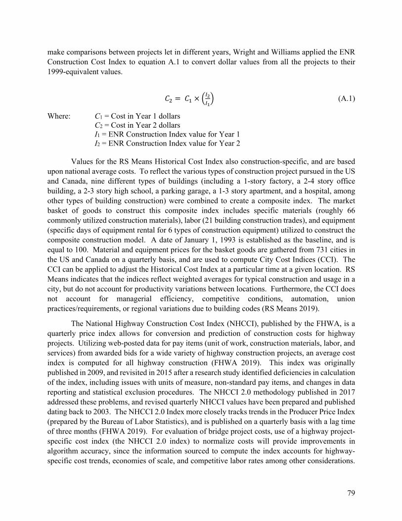
79

make comparisons between projects let in different years, Wright and Williams applied the ENR Construction Cost Index to equation A.1 to convert dollar values from all the projects to their 1999-equivalent values.

(A.1)

Where: C1 = Cost in Year 1 dollars C2 = Cost in Year 2 dollars I1 = ENR Construction Index value for Year 1 I2 = ENR Construction Index value for Year 2

Values for the RS Means Historical Cost Index also construction-specific, and are based

upon national average costs. To reflect the various types of construction project pursued in the US and Canada, nine different types of buildings (including a 1-story factory, a 2-4 story office building, a 2-3 story high school, a parking garage, a 1-3 story apartment, and a hospital, among other types of building construction) were combined to create a composite index. The market basket of goods to construct this composite index includes specific materials (roughly 66 commonly utilized construction materials), labor (21 building construction trades), and equipment (specific days of equipment rental for 6 types of construction equipment) utilized to construct the composite construction model. A date of January 1, 1993 is established as the baseline, and is equal to 100. Material and equipment prices for the basket goods are gathered from 731 cities in the US and Canada on a quarterly basis, and are used to compute City Cost Indices (CCI). The CCI can be applied to adjust the Historical Cost Index at a particular time at a given location. RS Means indicates that the indices reflect weighted averages for typical construction and usage in a city, but do not account for productivity variations between locations. Furthermore, the CCI does not account for managerial efficiency, competitive conditions, automation, union practices/requirements, or regional variations due to building codes (RS Means 2019).

The National Highway Construction Cost Index (NHCCI), published by the FHWA, is a quarterly price index allows for conversion and prediction of construction costs for highway projects. Utilizing web-posted data for pay items (unit of work, construction materials, labor, and services) from awarded bids for a wide variety of highway construction projects, an average cost index is computed for all highway construction (FHWA 2019). This index was originally published in 2009, and revisited in 2015 after a research study identified deficiencies in calculation of the index, including issues with units of measure, non-standard pay items, and changes in data reporting and statistical exclusion procedures. The NHCCI 2.0 methodology published in 2017 addressed these problems, and revised quarterly NHCCI values have been prepared and published dating back to 2003. The NHCCI 2.0 Index more closely tracks trends in the Producer Price Index (prepared by the Bureau of Labor Statistics), and is published on a quarterly basis with a lag time of three months (FHWA 2019). For evaluation of bridge project costs, use of a highway project-specific cost index (the NHCCI 2.0 index) to normalize costs will provide improvements in algorithm accuracy, since the information sourced to compute the index accounts for highway-specific cost trends, economies of scale, and competitive labor rates among other considerations.

80

In addition to the source data, an aggregate index is highly dependent on the method used to compute the value from each component index.

Three types of index formulas are commonly utilized in economics: The Laspeyres price index (Equation A.2), the Paasche price index (Equation A.3) and the Fisher Ideal index (Equation A.4). The weights assigned to each component index will help drive selection of the appropriate formula. The Laspeyres price index formula uses quantities of the base period (0) as weights, while the Paasche index utilizes quantities of the current period (t) as weights (FHWA 2019).

∑ , ,

∑ , , (A.2)

∑ , ,

∑ , , (A.3)

∑ , ,

∑ , ,

∑ , ,

∑ , , (A.4)

One key advantage of the NHCCI is that it utilizes the Fisher Ideal index. The Fisher Ideal

index accounts for the weights of both the base period and the current period, allowing the index to accommodate the effects of substitutions. Additionally, since the Fisher Ideal index is the geometric mean of the Laspeyeres price index and the Paasche price index, it to exhibit a “dual” property, with the product of a Fisher Ideal price index and a Fisher Ideal quantity index between the same two periods to equal the total change in value between the two periods (expressed in current dollars) (FHWA 2019). Limitations of the Laspeyres Index is that it can overstate the impact of price increases, and also understates the impact of price decreases as the distance from the base year increases, making it biased upward over time. The Paasche price index formula tends to exhibit the opposite bias, trending downward due to a substitution effect (FHWA 2019).

Other SHAs have prepared their own state-specific construction cost indices. The market basket utilized in each state can be tailored to suit agency preferences, as can the type of index. The form of the index formula utilized in these states can be one previously discussed, or another mathematical approach. A summary of selected state construction cost indices prepared as part of research sponsored by Minnesota DOT is presented in Table A.1. This study indicated that Minnesota DOT’s cost index was reflective of the NHCCI over a 15-year period (HDR 2018).

81

Table A.1: Summary comparison of state highway construction cost indices (from HDR 2018).

State Washington1 Montana2 Minnesota3 Iowa4 Ohio Utah5 Index Young Laspyres Laspyres Chained Fisher Modified

Laspeyres Frequency Quarterly Annually Quarterly,

Annually Quarterly, Annually

Quarterly Quarterly

Base Year 1990 1987 1987 1987 2012 Q1 2003 Categories 7 9 6 6 19 6 Item Category

Roadway Excavation Crushed

base Surfacing Hot mix

asphalt Concrete

pavement Structural

concrete Steel

reinforcing bar

Structural steel

Excavation Aggregate

base Surfacing Drainage Concrete Reinforcing

steel Bridge Traffic Miscellaneous

items

Excavation Reinforcing

steel Structural

steel Structural

concrete Concrete

pavement Plant-mix

bituminous pavement

Class 10 roadway and borrow, and embankment-in-place

Hot mix asphalt

pavement and shoulder mixes

Class ‘A’, class ‘B’, class ‘C’ pavements

Reinforcing steel

Structural steel

Structural concrete

Asphalt Aggregate

base Barrier Bridge

painting Curbing Drainage Earthwork Erosion

control Guardrail Landscaping Lighting Maintenance

of traffic Pavement

marking Pavement

repair PCC

pavement Removal Signalization Structures Traffic

control Unclassified

construction items

Roadway excavation

Hot mix asphalt

Concrete pavement (9-11” thick)

Reinforcing steel (coated)

Structural steel

Structural concrete

1 From WSDOT Highway Construction Costs, Washington DOT 2 From Jeong, D.H. et al. (2017). “Advanced Methodology to Determine Highway Construction Cost Index (HCCI).” Montana DOT. 3 From Minnesota DOT 4 From “Price Trend Index for Iowa Highway Construction.” Iowa DOT, Office of Contracts 5 From “UDOT Construction Cost Indices.” Utah DOT

Since cost indices are based on data from construction projects, there are no values

available for future years. To estimate the adjusted cost of a project for a future year, the index data can be extrapolated using regression techniques. For early work using the NCDOT BMS, Abed-al-Rahim and Johnston (1995) used the FHWA Structures Index to convert bridge cost data to a common year. The first step of the conversion was used to bring the bridge project costs to a common base year, using an equation similar to Equation A.1. The limitation to this method is that the base year must fall within the range of years from which the construction index data is sourced. To bring these common base year costs to present or future values, Abed-al-Rahim and Johnston

82

(1995) developed a linear regression equation from the construction index data that extrapolated future year index values with a relatively good fit (R2 = 0.84). The future year index value found in Equation A.5 can be plugged back into Equation A.1 to solve for the cost in Year 2 dollars.

, 102.21 3.9 (A.5)

Where: IND(YF,YB) = Cost index for future year YF and base year YB YB = Base year YF = Future year

A.3 Cost Prediction Modeling Approaches Demand for accurate cost forecasting methods for highway projects has prompted several state transportation agencies to fund research projects on cost prediction modeling. In this section, an overview of several different approaches is presented, along with background information required to develop these models. This section also discusses how predictions from the models can be implemented into a bridge management system.

A.3.1 Types of Variables Variables can be classified by the way their data is recorded. Continuous or quantitative variables are numerical values that can be measured at any point along a range of possible values. The granularity of the data is only limited by the precision of the instrument which provided the original measurement. Many variables included in a BMS, such as daily traffic, length, and width, can be considered continuous or quantitative variables. Discrete variables can also be expressed as numerical values, however there is no smooth transition between values. One example of this would be the number of spans for a bridge. This field can only be expressed in whole numbers, since half-span bridges do not exist. The distinction between continuous and discrete numerical variables can become blurred whenever the precision of the continuous variable is limited or the steps between the discrete values become very small (Tabachnick and Fidell 2006).

Discrete variables can also describe non-numerical qualitative data. In a BMS database, this could be deck material, functional classification of the route, or whether the bridge crosses over water or a grade change. Dichotomous variables have only two possible values (Tabachnick and Fidell 2006). Categorical variables can be used to designate discrete variables into grouped categories.

A.3.2 Types of Models The cost for bridge replacement projects can be estimated through traditional cost estimation or through aggregated statistical modeling. Traditional cost estimates are calculated by listing all of the work items and multiplies their quantities by a unit price. The sum of all the costs for the work items is the estimated value for the complete project. Aggregated statistical modeling uses

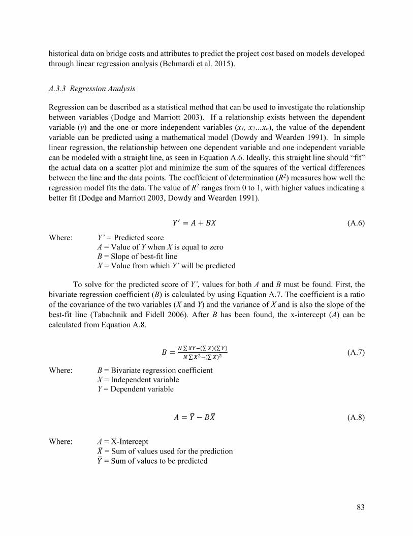
83

historical data on bridge costs and attributes to predict the project cost based on models developed through linear regression analysis (Behmardi et al. 2015).

A.3.3 Regression Analysis Regression can be described as a statistical method that can be used to investigate the relationship between variables (Dodge and Marriott 2003). If a relationship exists between the dependent variable (y) and the one or more independent variables (x1, x2…xn), the value of the dependent variable can be predicted using a mathematical model (Dowdy and Wearden 1991). In simple linear regression, the relationship between one dependent variable and one independent variable can be modeled with a straight line, as seen in Equation A.6. Ideally, this straight line should “fit” the actual data on a scatter plot and minimize the sum of the squares of the vertical differences between the line and the data points. The coefficient of determination (R2) measures how well the regression model fits the data. The value of R2 ranges from 0 to 1, with higher values indicating a better fit (Dodge and Marriott 2003, Dowdy and Wearden 1991).

(A.6)

Where: Y’ = Predicted score A = Value of Y when X is equal to zero B = Slope of best-fit line X = Value from which Y’ will be predicted

To solve for the predicted score of Y’, values for both A and B must be found. First, the bivariate regression coefficient (B) is calculated by using Equation A.7. The coefficient is a ratio of the covariance of the two variables (X and Y) and the variance of X and is also the slope of the best-fit line (Tabachnik and Fidell 2006). After B has been found, the x-intercept (A) can be calculated from Equation A.8.

∑ ∑ ∑

∑ ∑ (A.7)

Where: B = Bivariate regression coefficient X = Independent variable Y = Dependent variable

(A.8)

Where: A = X-Intercept = Sum of values used for the prediction = Sum of values to be predicted

84

Multiple regression is an extension of bivariate regression in which more than one independent variable is used to predict values of a dependent variable (Tabachnik and Fidell 2006). For example, in the case of this project, it is useful to predict the construction cost of a bridge replacement project (dependent variable) based on the several independent variables available in the data set, such as structure length, number of spans, material, or design type. The multiple linear regression equation (A.9) is an extension of the bivariate regression equation (A.6) that is designed to be used with more than just one independent variable. Each independent variable has its own regression coefficient, which is used to bring the predicted values of Y as close as possible to the values from the data set and maximize the correlation between the predicted and obtained values for Y.

⋯ (A.9)

Where: = Predicted score for dependent variable A = Value of Y when all X values equal zero Bn = Regression coefficient for n-th variable Xn = n-th independent variable k = Number of independent variables

Collinearity is a consideration for regression equations that involve multiple independent variables. This condition exists when there is a high amount of correlation between two or more predictor variables. In layman’s terms, the two variables are measuring the same thing (or highly interrelated things). In a multiple regression analysis, collinearity that is not addressed will cause variables that truly affect the dependent variable to not appear in the regression equation while the other predictor variable may have a large impact on the equation. There are several ways to deal with collinearity between variables. After the collinear variables have been identified, the two variables can be combined into one single variable by converting each of the variables into a z score and them using the sum of the z scores as the total for the new variable. Another approach is to use a factor analysis that will identify the set of factors within the collinear variables and use the factors in the regression analysis (Cramer and Howitt 2004). Collinearity can also be addressed by removing one of the collinear variables from the regression model.

A.3.4 Regression Tree Analysis Decision trees are a useful tool to describe data and to develop models to support decision analysis (Pratt et al. 1995). Models resulting from decision tree analysis predict the value of a root or target variable using input variables. The source dataset is split into nodes from the root node based upon classification features using recursive partitioning, where the subgroups are split in a manner that classifies them into groups (Denison et al. 2002). In binary recursive partitioning, the tree is split into two notes: a group that has the same features as the target value, and a group that does not, based upon a decision criteria (which can be viewed as a yes/no question) at each node. The recursive partitioning is halted when splitting a subset no longer improves the quality of the model or some pre-determined stopping criteria are met. An example of a two-dimensional input space

85

partitioned into five regions using recursive binary partitioning is shown in Figure A.6a, with the corresponding tree structure shown in Figure A.6b.

B

A

C

E

D

Θ4Θ1

Θ2

Θ3

x1

X1>Θ1

X2>Θ3

X1≤ Θ4

X2≤ Θ2

A B C D E

Figure A.6a: Example of two-dimensional input space partitioned into five regions (from Bishop 2006)

Figure A.6b: Corresponding binary tree (from Bishop 2006)

Regression tree analysis (also called classification and regression tree, or C&RT, analysis)

is one form of decision tree analysis (Brieman et al.1984). In regression tree analysis, the regression builds a model in the form of a tree structure to result in a predicted outcome that is a real number. The regression model is constructed to reduce the residual sum of squares (Takezawa 2006). Through this process, the factors most significantly influencing the dependent variable are identified, and the data is incrementally broken down into smaller subsets based upon the optimized decision criteria. The resulting decision tree has a single root node, and two or more decision nodes and leaf notes, as shown in Figure A.6b. The root node corresponds to the independent variable identified as the best predictor. Decision nodes represent values for other independent variables tested, and have two or more branches. “Greedy optimization” is utilized, starting at a single root node, then adding nodes one at a time. Following the addition of each node, the candidate regions are split using joint optimization using an exhaustive search algorithm, local averaging of data, and identification of the splitting choice with the smallest residual sum-of-squares error (Bishop 2006).

The C&RT method is nonparametric and nonlinear, and therefore a frequency distribution of variables is not assumed, and the relationships between the dependent and independent variables are not assumed to be linear. Advantages of C&RT methods include the simplicity of the final model (and its easy interpretation), and its usefulness for identifying interactions between variables. Stopping criteria can be established as a limit on tree depth, an identical distribution of predictors, or a single observation present in a terminal leaf node. Overfitting of the model is controlled by removing nodes from the tree if the model accuracy is not improved (Bishop 2006).

86

If a decision node, T, is subdivided at T0, T ⸦ T0 is defined as a subtree if T0 can be obtained by collapsing internal nodes by combining corresponding subregions. Leaf nodes are defined as τ = 1, … |T|, with corresponding regions designated as Rτ, with an input space of Nτ datapoints and |T| denoting the total number of leaf nodes. The optimal prediction region Rτ can be given as Equation A.10, along with the corresponding contribution to the residual sum of squares (Equation A.11) and the pruning criterion (Equation A.12) (Bishop 2006):

1

∈

(A.10)

∈

(A.11)

| |

| |

∈

(A.12)

Where λ = a regularization parameter determining the trade-off between the overall residual sum-of-squares area and the complexity of the model, which is measured by | |. The value of λ is selected through cross-validation, described in the following section.

A.3.5 Cross-validation Cross-validation is performed when an available dataset (or the dataset to be used for validation) is small, and may not provide an adequate estimate of predictive performance. In cross-validation techniques, a proportion of the available data is used for training the model, while the remaining data not used to train the model is utilized to assess the model performance. Multiple cross-fold validation is illustrated in Figure A.7, where equals the number of groups or ‘folds’ (in this case, 4). In this example, the available data is partitioned into 4 groups. A subset of the data developed by 1 of the groups are utilized to train a set of models, which are subsequently evaluated using the remaining group (indicated in figure A.7 in gray). The process is repeated until all combinations of subsets are utilized as the remaining group. The value of is often selected so that the size of each group is large enough to be statistically representative of the broader dataset. Other approaches for selecting include selection of a fixed number, often 5 or 10, although there is no formal rule (Kuhn and Johnson 2013). After each iteration, the evaluation

87

score is retained, and the model discarded. The accuracy of the model is taken as the mean accuracy computed from each fold.

Run 1

Run 2

Run 3

Run 4

Figure A.7: k-fold cross validation (from Bishop 2006)

A.3.6 Use of Cost Prediction Models in Bridge Management Systems All SHAs are required to comply with the Intermodal Surface Transportation Efficiency Act of 1991 by implementing a BMS that logs bridge data and considers the costs of repairing, rehabilitating, or replacing deficient bridges (Abed-al-Rahim and Johnston 1995). The three alternatives are typically evaluated based on a variety of considerations, including ownership and user costs, as well as budget constraints and the preferences of state/local personnel. The decision to replace a functionally obsolete or deteriorated bridge will bring the user cost back to zero at the beginning of the new bridge’s service life (Chen and Johnston 1987).

Currently, the NCDOT BMS computes the bridge replacement cost using the bridge deck area and a unit cost based on functional classification. The deck width and length for a new bridge is calculated based on the desired level of service. Design and planning of the new structure is estimated as a fixed percentage of the base construction cost. Costs associated with roadway improvements can be added onto the subtotal as a fixed amount (Chen and Johnston 1987).

A.4 Existing Cost Prediction Models The term “conceptual estimate” was first recognized in 1975 by a federal government publication that urged construction managers to familiarize themselves with the technique (Collier 1984). Around this time, computerized bridge management systems were being developed to catalog bridge inspection data and prioritize bridge maintenance needs (Chen and Johnston 1987). The ability of a BMS to estimate the cost to replace a bridge helps the system users to evaluate whether it is more feasible to repair, rehabilitate, or replace the bridge (Abed-al-Rahim and Johnston 1995). By 1992, these systems had been implemented by several states, providing these agencies with the ability to consider user costs, owner costs, level-of-service goals, or life-cycle activity profiles to

88

estimate replacement costs (OECD 1992). The following sections identify and discuss some of the cost modeling approaches developed for North Carolina bridges and for bridge systems in other states.

A.4.1 Use of Cost Prediction Models in North Carolina At the time of the research conducted by Chen and Johnston (1987), NCDOT estimated bridge replacement costs with a fixed unit cost of $43 per square foot of deck area. This same unit cost would be applied to all bridge replacement projects without regard to project size, location, design, or traffic volume. Further research was conducted by Abed-al-Rahim and Johnston in the early 1990s to develop models that will produce a unit cost based on different project characteristics. As mentioned previously, additional research by NCDOT focused on evaluation of PE costs and development of models (Hollar et al. 2013).

A.4.1.1 Abed-al-Rahim and Johnston (1995)

In 1995, North Carolina State University (NCSU) researchers developed a framework for the NCDOT to estimate unit costs for bridge replacement projects based on bridge-specific factors cataloged in a BMS database. Abed-al-Rahim and Johnston (1995) also developed models that would predict new bridge characteristics. The North Carolina Bridge Index (NCBI) contained the total bridge project cost for each bridge record, as well as the costs for preliminary engineering, construction, and roadway improvement. Miscellaneous items, such as right-of-way purchases, field operations, and legal fees were estimated by subtracting the three cost categories from the total project cost, as seen in Equation A.13.

(A.13)

Where: TOTCOST = Total project cost

MISCCOST = Miscellaneous costs STRCOST = Bridge structure cost ROADCOST = Roadway improvement cost ENGCOST = Engineering cost

Abed-al-Rahim and Johnston used the FHWA Structures Index for North Carolina to

convert costs to a present value. Equation A.1 was used to convert dollar values from the year of construction (YC) to the latest available year (YL), using 1987 as a base year (YB). It was also possible to extrapolate data from the FHWA Index for future years, as shown in Equation A.2, which was developed based upon linear regression conducted by Abed-al-Rahim and Johnston (1995). The linear model yielded an R2 value of 0.84. After using Equation 2.2 to determine the future year (FY) cost index, Equation 2.1 was used to calculate the future year cost.

Before a detailed bridge design is created, specific bridge characteristics such as structure length, deck width, and maximum span length are typically not known with certainty. These

89

variables will have an impact in the overall replacement cost of a bridge, especially in cases where there is a large change in one of these characteristics for the new bridge relative to the old bridge (Abed-al-Rahim and Johnston, 1995). A set of models that can predict these new bridge characteristics based on those of the existing bridge can help estimators identify structures that would undergo a relatively large increase in size and therefore have a potentially higher cost to replace. Using the Generalized Linear Method (GLM), Abed-al-Rahim and Johnston (1995) performed regression analysis to develop an equation that could be used to predict new bridge length based on several existing bridge parameters. With new bridge length as the sole dependent variable, Abed-al-Rahim and Johnston considered several independent variables, such as existing bridge length, waterway adequacy, and under-clearance ratings. Ultimately, old bridge length was the independent variable that provided the best fit (R2=0.9854), so the following regression equation (A.14) was developed:

8.45 1.013 1 (A.14)

Where: NBLENNC = New bridge length based on NC data (in meters) L1= Old bridge length (in meters)

Abed-al-Rahim and Johnston also utilized the FHWA Expansion Factor to predict new

bridge length. These factors are based on nationwide averages of new bridge length as a function of existing bridge length. To use the expansion factor, Abed-al-Rahim and Johnston (1995) took various original lengths from the curve (Fig. A.8) and identified corresponding expansion factors. Multiplying the original bridge lengths by the respective expansion factors yielded a list of new bridge lengths. A linear regression was performed with the original lengths (independent variable) and new lengths (dependent variable) to generate a regression equation (A.15).

Figure A.8: FHWA length expansion factor graph (from Abed-Al-Rahim and Johnston 1995)

90

7.32 1.032 1 (A.15)

Where: NBLENUS = New bridge length based on US data (in meters) L1 = Old bridge length (in meters)

Abed-al-Rahim and Johnston (1995) used Equation A.16 to estimate the new bridge out-

to-out deck width, with the predicted clear deck width for the new bridge (NBCDWi) determined in OPBRIDGE by considering future level-of-service and ADT needs. OPBRIDGE was a computer program developed by Al-Subhi et al. (1989) to forecast and prioritize future bridge replacement projects. The equation computes the difference between current out-to-out width and current deck width, adding it to the predicted clear deck width to provide the predicted out-to-out width for the new bridge. This assumes that the difference in width between out-to-out and clear deck widths will remain the same for the new bridge.

(A.16)

Where: NBWIDi = Predicted out-to-out width for new bridge i NBCDWi = Predicted clear deck width for new bridge i WIDTHi = Out-to-out width for bridge i that is to be replaced CDWi = Clear deck width of bridge i that is to be replaced

As one of the significant factors in predicting replacement cost, a bridge’s maximum span length can also be predicted by its original maximum span length, waterway adequacy rating, structure length, and number of spans (Abed-al-Rahim and Johnston 1995). This research team found that it was best to create two separate models for bridges over waterways and bridges over grade separations. Both models used old total length and maximum span of the bridge being replaced as independent variables and applied a logarithmic transformation to allow the models to meet the two assumptions for regression analysis: 1) Normal distribution of residuals, and 2) Variance is consistent along the regression line.

After developing the two models, the research team was unable to prove that the coefficients in both equations were statistically different. The dataset of bridges used by Abed-al-Rahim and Johnston included 442 waterway crossings but only 39 grade separation crossings. Using a single, logarithmic-transformed model instead of two separate models yielded an R2 value of 0.53, resulting in Equation A.17. Both Equation A.17 and Figure A.9 show that new maximum span length are predicted to be shorter if the original span length is greater than 75 feet. Conversely, bridges with an original maximum span length less than 75 feet are predicted to have an increase in maximum span length for the new bridge (Abed-Al-Rahim and Johnston 1995).

2 4.31 1 . 1 . (A.17)

Where: MAXSPAN2 = Predicted maximum span length MAXSPAN1 = Original maximum span length L1 = Original bridge length

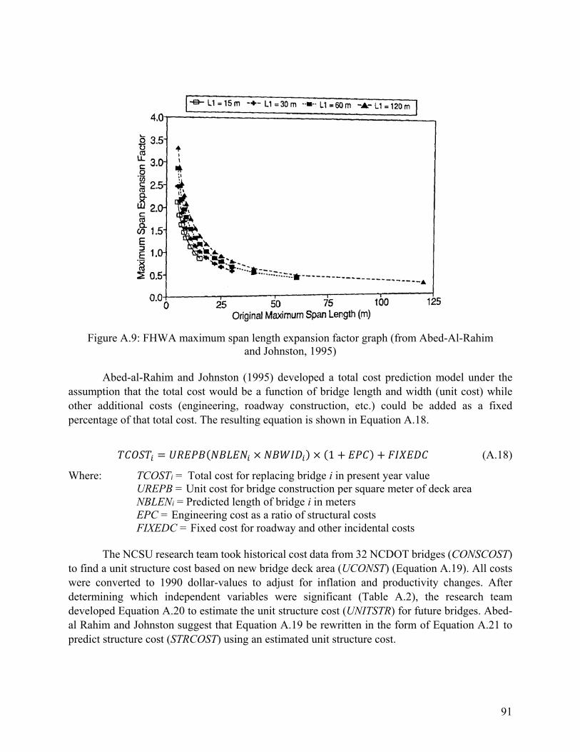
91

Figure A.9: FHWA maximum span length expansion factor graph (from Abed-Al-Rahim

and Johnston, 1995) Abed-al-Rahim and Johnston (1995) developed a total cost prediction model under the

assumption that the total cost would be a function of bridge length and width (unit cost) while other additional costs (engineering, roadway construction, etc.) could be added as a fixed percentage of that total cost. The resulting equation is shown in Equation A.18.

1 (A.18)

Where: TCOSTi = Total cost for replacing bridge i in present year value UREPB = Unit cost for bridge construction per square meter of deck area NBLENi = Predicted length of bridge i in meters EPC = Engineering cost as a ratio of structural costs FIXEDC = Fixed cost for roadway and other incidental costs The NCSU research team took historical cost data from 32 NCDOT bridges (CONSCOST) to find a unit structure cost based on new bridge deck area (UCONST) (Equation A.19). All costs were converted to 1990 dollar-values to adjust for inflation and productivity changes. After determining which independent variables were significant (Table A.2), the research team developed Equation A.20 to estimate the unit structure cost (UNITSTR) for future bridges. Abed-al Rahim and Johnston suggest that Equation A.19 be rewritten in the form of Equation A.21 to predict structure cost (STRCOST) using an estimated unit structure cost.

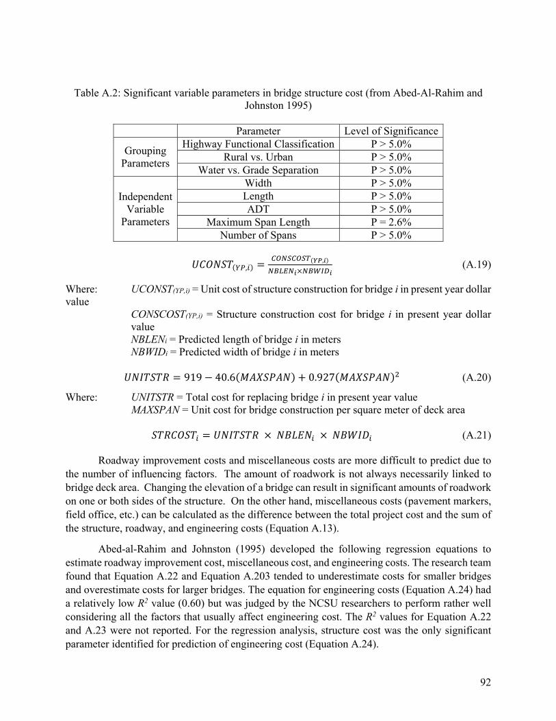
92

Table A.2: Significant variable parameters in bridge structure cost (from Abed-Al-Rahim and Johnston 1995)

Parameter Level of Significance

Grouping Parameters

Highway Functional Classification P > 5.0% Rural vs. Urban P > 5.0%

Water vs. Grade Separation P > 5.0%

Independent Variable

Parameters

Width P > 5.0% Length P > 5.0% ADT P > 5.0%

Maximum Span Length P = 2.6% Number of Spans P > 5.0%

,, (A.19)

Where: UCONST(YP,i) = Unit cost of structure construction for bridge i in present year dollar value

CONSCOST(YP,i) = Structure construction cost for bridge i in present year dollar value

NBLENi = Predicted length of bridge i in meters NBWIDi = Predicted width of bridge i in meters 919 40.6 0.927 (A.20)

Where: UNITSTR = Total cost for replacing bridge i in present year value MAXSPAN = Unit cost for bridge construction per square meter of deck area (A.21) Roadway improvement costs and miscellaneous costs are more difficult to predict due to the number of influencing factors. The amount of roadwork is not always necessarily linked to bridge deck area. Changing the elevation of a bridge can result in significant amounts of roadwork on one or both sides of the structure. On the other hand, miscellaneous costs (pavement markers, field office, etc.) can be calculated as the difference between the total project cost and the sum of the structure, roadway, and engineering costs (Equation A.13).

Abed-al-Rahim and Johnston (1995) developed the following regression equations to estimate roadway improvement cost, miscellaneous cost, and engineering costs. The research team found that Equation A.22 and Equation A.203 tended to underestimate costs for smaller bridges and overestimate costs for larger bridges. The equation for engineering costs (Equation A.24) had a relatively low R2 value (0.60) but was judged by the NCSU researchers to perform rather well considering all the factors that usually affect engineering cost. The R2 values for Equation A.22 and A.23 were not reported. For the regression analysis, structure cost was the only significant parameter identified for prediction of engineering cost (Equation A.24).

93

177,900 1,198,500 (A.22)

Where: ROADCOST = Roadway improvement cost NBWID = Predicted bridge width in meters 0.56 42,500 364,000 (A.23)

Where: MISCCOST = Miscellaneous costs STRCOST = Bridge structure cost NBWID = Predicted bridge width in meters 65,384 0.136 (A.24) Where: STRCOST = Bridge structure cost ENGCOST = Engineering cost A.4.1.2 Hollar et al. (2013) Preliminary engineering costs for a bridge replacement project are typically estimated as being a fixed percentage of the total project cost. This technique does not address project-specific parameters that would cause PE costs to increase. According to the 2008 auditor’s report for schedule and budget performance of NCDOT highway projects, PE costs for a set of 292 highway projects completed between April 1, 2004 and March 31, 2007 typically increased by 59% over the original estimated amount. This specific area had not received much attention from researchers due to the lack of reliable information available for PE costs (Hollar et al., 2013).

Hollar et al. (2013) compiled a database of 461 NCDOT bridge projects from several sources, such as online bid tabulations and construction plans, National Bridge Inventory System (NBIS) data, 12-month letting lists, meeting minutes, and funding authorizations. The bridges in the compiled database were usually three-span, two-lane concrete structures that crossed water features in rural areas. The dependent variable for this analysis was the ratio of actual PE cost to the estimated Statewide Transportation Improvement Program (STIP) construction cost. The research team used estimated costs instead of actual costs because estimators would not know the actual cost of a project during the conceptual planning stage. Using the correct PE cost ratio for a project would reduce the likelihood of cost escalation. The distribution of the PE cost ratio for the 461 NCDOT bridge projects ranged from 0.8% to 152% of estimated construction cost. The shape of the distribution was skewed to the left and needed to be transformed to improve normality to satisfy linear regression assumptions (Hollar et al. 2013).

The 461 database projects were divided into a modeling set of 391 projects and a validation set of 70 projects. The validation projects were used to test and quantify the model’s performance in predicting the ratio of PE to STIP. Each candidate model was tested over the validation set by comparing the predicted PE cost values to the actual historical values for those projects. The models with lowest Mean Absolute Percentage Error (MAPE) and Average Absolute Error (AAE) were preferred over models with higher error values (Hollar et al. 2013).

94

The response variable (PE cost ratio) was transformed by applying an exponential power and using the Box-Cox procedure to identify the optimal transformation to get normality. In this case, the cubed root of the response variable was used to attain normality, which was then verified using a goodness-of-fit test. Since the dependent variables were normalized using the power transformation, results had to be transformed back using Equations A.25, A.26, and A.27. The equations were solved using a variance value of 0.0229 for the data set (Hollar et al. 2013).

. . . (A.25)

Where: E.M.R. = Estimated Median Response

. . 1 1 13 / 2 (A.26)

Where: T.C.F. = Transformation Correction Factor var = Variance

. . . . (A.27)

Where: E.M.R. = Estimated Median Response T.C.F. = Transformation Correction Factor The one-way ANOVA technique was applied to the 16 categorical variables in the compiled database to identify those which were statistically significant. The seven significant categorical variables are listed in Table A.3. The two categorical variables with the highest level of influence on the cubed root of the PE cost ratio were year-related. The researchers assumed that any fluctuations in STIP estimated costs over time would be mirrored by the actual PE costs, so these two variables were not used as predictor variables in the analysis (Hollar et al. 2013).

Table A.3: Statistically significant categorical variables (Hollar et al. 2013)

Categorical Variable R2 F-value p-value Year of letting 0.3037 20.83 <0.0001 Year of environmental doc. approval 0.1220 3.47 <0.0001 Road system 0.0443 8.80 0.0002 Project construction scope 0.0322 6.45 0.0017 Geographical area of state 0.0361 4.84 0.0026 Division 0.0728 2.28 0.0068 Design live load 0.0302 3.00 0.0185

To determine which of the numerical variables should be used in the regression model,

Hollar et al. (2013) used the Pearson correlation coefficients and p-values to identify which variables were statistically significant. The correlation coefficient, which ranges between -1 to +1, indicates the strength of the correlation with the cubed root of PE cost ratio. The sign of the coefficient reflects whether the independent and response variables are positively correlated

95

(positive slope) or are negatively correlated (negative slope). Table A.4 contains the eight numerical independent variables that were determined to be statistically significant.

Table A.4: Pearson correlation coefficients for numerical variables (Hollar et al. 2013)

Numerical Independent Variable Pearson Coefficient p-value Project length -0.3263 <0.0001 STIP-estimated construction cost -0.3130 <0.0001 ROW cost to STIP-estimated Construction cost

+0.3089 <0.0001

Structure length -0.1944 <0.0001 Roadway percentage of construction cost

-0.1849 <0.0001

Spans in primary unit -0.1766 <0.0001 Horizontal clearance for loads -0.1592 0.0006 PE duration after environmental document approval

-0.1053 0.0237

After selecting the statistically-significant categorical and numerical variables for the linear

regression, the research team used the GLMSELECT procedure within SAS to create a multiple linear regression (MLR) model. Excluding all date-related variables, the completed MLR model achieved an adjusted R2 value of 0.2745 using the following variables:

1. ROW cost to STIP-estimated construction cost (Numerical) 2. Roadway percentage of construction cost (Numerical) 3. STIP-estimated construction cost (Numerical) 4. Bypass detour length (Numerical) 5. Project construction scope (Categorical) 6. NCDOT division (Categorical) 7. Geographical area of state (Categorical) 8. Responsible party for the planning document (Categorical) When applied to the data set of 70 projects, the MLR provided a MAPE of 0.1889. This

was compared to the MAPE of 0.9137 that was achieved by a single-point estimate using the mean PE cost ratio of the remaining 391 projects. This single-parameter estimating method is commonly used by the NCDOT to estimate PE costs and also served as a baseline target to measure the MLR model’s prediction capability. After obtaining the regression coefficients (Table A.5), Equation A.28 can be used to find the predicted cube root of the PE cost ratio to STIP construction cost (Hollar et al. 2013).

96

Table A.5: Regression coefficients for MLR model (Hollar et al. 2013)

Parameter Coefficient Intercept β0 0.6471 x1 NCDOT division = D12 and project construction scope = new

location; 1 if true, 0 if false β1 -0.1657

x2 NCDOT division = D06 and responsible party for the planning document = DOT; 1 if true, 0 if false

β2 -0.1087

x3 Geographical area of state = very mountainous and responsible party for the planning document = DOT; 1 if true, 0 if false

β3 0.0701

x4 ROW cost to STIP-estimated construction cost β4 0.2909 x5 STIP-estimated construction cost if NCDOT division = D12 β5 4.45 × 10-8

x6 Roadway percentage of construction cost multiplied by STIP-estimated construction cost

β6 -1.88 × 10-7

x7 Bypass detour length if NCDOT division = D07 β7 -0.0159

(A.28) Ideally, the MLR model would follow a 45-degree positive slope, which would mean that

the predicted values would be close to the actual values. The slope of the MLR model is positive but smaller than the ideal slope. Compared to the mean-value of the PE cost ratio for the set of 391 projects, the MLR model overestimated PE cost ratios at the lesser percentages (<20%) and underestimated ratios at higher percentages (>35%). The MLR model had a MAPE value of 42.7%. Compared to the mean value’s MAPE of 48.7%, the MLR had slightly better performance over the single-point estimator (Hollar et al. 2013).

Despite the relatively high prediction error percentage for the MLR model (42.7%), the results of the modeling confirmed the research team’s assertions that PE costs for bridge projects were often underestimated. The historical mean reported by Hollar et al. (2013) for NCDOT bridge projects was 27.8%, which was greater than the WSDOT estimate of 10.3%, VDOT estimate range of 8-20%, and Georgia DOT estimate range of 6-12%. The data used to create the model should be readily available for most state agencies. Hollar et al. found that state agency procedures and processes could compromise the quality of PE cost data. In the case of this study, the research team found that PE costs were often charged as an overhead burden and not accurately assigned to the individual bridge projects. For this reason, it is important that databases should be expanded and updated often to create a solid data set for creating regression models (Hollar et al. 2013).

In addition to suggesting means to improve the quality of PE cost data recording procedures, Hollar et al. (2013) also recommended that future researchers analyze PE costs in terms of monetary units instead of ratios. To do this, it is necessary to convert all costs to a common year. The research team expressed a need for future research into reasons why PE costs were driven up for projects, such as the instances where the project PE cost ratio was 152% of the construction

97

cost. An analysis of case studies may provide qualitative data on how certain factors increase PE costs (Hollar et al. 2013).

A.4.2 Use of Cost Prediction Models in Other State Agencies

Since bridge maintenance and replacement programs are managed by SHAs, many of these agencies have funded research projects that determine the most effective way to forecast bridge replacement costs that work best for the state bridge inventories. Publications exist on the many different approaches researchers have employed to create state-specific prediction models. The techniques used by researchers to develop cost prediction models for Indiana DOT and Texas DOT are covered in more detail in the following sections.

A.4.2.1 Indiana Department of Transportation Saito et al. (1991) developed a series of regression models for predicting costs for bridge replacement projects in Indiana. A dataset of 279 Indiana Department of Transportation (INDOT) bridges replaced between 1980 and 1985 was compiled by the researchers. Bridge attributes used for the model, such as structure length, deck width, vertical clearance, approach length, and earthwork needed, could be easily identified by inspectors and included in the database. Cost data were the dependent variables for the study, and all prices were converted to 1985 values using the FHWA construction price index. Cases where multiple bridges were included on one contract or where replacement costs were extremely high or low were removed from the data set to avoid influence from outliers.

To develop the replacement cost model, the ANOVA (analysis of variance) technique was used to determine the effect that the independent variables, such as structure length, deck width, and number of spans, had on the actual contract costs. SPSS and SAS statistical software packages were then used to take the results of the ANOVA and develop a regression model. The ANOVA was done based on three primary classification factors that were currently being used by INDOT to estimate bridge replacement cost: superstructure type, substructure type, and highway type. At the time of the study, the FHWA required state agencies to provide separate unit costs for each of the different highway types and superstructure types (Saito et al. 1991).

The ANOVA test confirmed that both superstructure and substructure types were statistically significant (5% level) in predicting unit substructure cost and that both factors should be used to generate estimates. A separate ANOVA test was performed for approach construction costs, but with total contract costs instead of unit costs. This test was based on two factors: amount of earthwork (small, medium, or large) and approach length (short, medium, or long). Results from this ANOVA test showed that amount of earthwork and approach length can and should be used as factors in predicting approach construction costs (Saito et al. 1991).

The results from both ANOVA tests were then used by the research team to develop bridge replacement cost models that required as few independent variables as possible. The models developed by Saito et al. (1991) were nonlinear and log-linear in nature, and used predictor

98

variables that could be easily determined by engineers on the site, such as designed structure length, width, and vertical clearance. Results from ANOVA and the scatter plots showed that regressions could be done for the four cost categories (superstructure, substructure, approach, and other costs) using a multiplicative regression model, shown in Equation A.29. Usage of the multiplicative model works under the same logic as unit costs, where structure length and width are multiplied by that unit price to determine the total cost. Since the regression coefficients are fixed values, Saito et al. (1991) cautioned users of this model (INDOT) against using it for bridges that were outside the data range used in the creation of the prediction models.

… (A.29)

Where: Y = Dependent Variable (Replacement Cost) Xn = Independent Variable Βn = Regression coefficient ϵ = Error coefficient

With a non-linear regression, it is possible to transform the raw data to see if it is possible to perform a linear regression analysis. Equation A.30 was transformed into Equation A.31 using log10 transformation (Saito et al. 1991). The new equation could be used provided that it met the key assumptions of linear regressions (Nau 2009):

1. Linearity and additivity of relationship between independent and dependent variables 2. Statistical independence of errors 3. Heteroscedasticity (constant variance) 4. Normality of error distribution

If the transformed model met all of the four key assumptions, it was returned to the non-linear form shown in Equation A.30. Once this was performed, the non-linear cost model and transformed log-linear model were compared to see if one model is preferable for use in estimating replacement costs. In making the comparison, the research team assumed that error terms were independent, variance was constant along the regression line, linearity of the model, and the residuals were distributed normally. When comparing the two models, residual plots were used to test the constancy of variance. Normal probability plots of the residuals were used to test normality of the error term distribution (Saito et al. 1991).

⋯ (A.30)

Where: Y’ = log10(Y) β'

0 = log10(β0) X’i = log10(Xi) ϵ’ = log10(ϵ)

10 … (A.31)

Log-linear models were developed to predict bridge replacement, superstructure, substructure, approach, and “other” costs. Separate equations were developed for significant categorical variables alongside an overall equation for all bridge types. The log-linear equations

99

for bridge replacement total cost (BRTC) (Table A.6), superstructure cost (Table A.7), substructure cost (Table A.8), and approach cost (Table A.9) were validated with a set of bridge data for projects between January and June 1986. Of the 37 bridges in the validation set, only 26 of the bridges had complete cost data for the other cost components while the remaining 11 bridges only had information on total project cost. After adjusting the predicted values to 1986-dollar equivalents, Saito et al. (1991) found that the models were reasonably precise. Cost values for these equations were rounded to the nearest $1,000 while bridge length (BL), deck width (DW), and vertical clearance (VC) were reported in feet.

Table A.6: BRTC regression equations (in 1985 dollars)

Component Type Model R2 F Value n Other All types OTHC = 0.0721(BL)0.696(DW)0.932 0.524 100.60 186

Bridge Total

All types BRTC = 0.155(BL)0.903(DW)0.964 0.951 1861.28 196 RC Slab & Box Beam

BRTC = 0.0781(BL)0.748(DW)1.319 0.874 380.74 113

Concrete I-Beam BRTC = 1.255(BL)0.809(DW)0.534 0.913 205.34 42 Steel Beam BRTC = 0.128(BL)0.785(DW)1.210 0.971 317.50 22 Steel Girder BRTC = 0.353(BL)1.015(DW)0.603 0.950 150.91 19

Table A.7: Superstructure cost regression equations (in 1985 dollars)

Type Model R2 F Value n

All types SUPC = 0.0107(BL)1.122(DW)1.084 0.524 1861.28 196

RC Slab & Box Beam SUPC = 0.0137(BL)1.001(DW)1.161 0.874 380.74 113 Concrete I-Beam SUPC = 0.0330(BL)0.907(DW)1.043 0.913 205.34 42 Steel Beam SUPC = 0.0102(BL)1.120(DW)1.117 0.971 317.50 22 Steel Girder SUPC = 0.8550(BL)0.906(DW)0.747 0.950 150.91 19

Table A.8: Substructure cost regression equations (in 1985 dollars)

Type Model R2 F Value n

All types SUBC = 0.00168(BL)0.906(DW)1.255(VC)0.487 0.725 168.35 196

Steel Girder SUBC = 0.00354(BL)0.744(DW)1.205(VC)0.515(T)0.156 0.751 143.62 196 Note: T = 1 for solid stem piers, T = 0 for pile-type piers

100

Table A.9: Approach cost regression equations (in 1985 dollars)

Models R2 F Value n APC = 0.769(APL)0.823 0.566 248.08 192 APC = 39.876(EW)0.378 0.633 328.20 192 APC = 4.715(APL)0.403(EW)0.250 0.696 215.93 192

Note: APL = Approach cost and EW = Earthwork (in 100CY)

A.4.2.2 Texas Department of Transportation Chou et al. (2005) developed a probabilistic cost estimation tool for the Texas Department of Transportation (TxDOT). An analysis of TxDOT bridge data from 2001 to 2003 showed that there were 22 major work items in a bridge project that accounted for roughly 80.2% of the total cost (Table A.10). The estimation tool was created under the assumption that estimators would be able to control at least 80.2% of the total project cost.

The unit cost for each work item was expressed as a cost per lane-kilometer. Equation A.32 was used to calculate the total project cost by adding up the unit costs for all 22 major work items. The sum of the major work item unit costs was divided by 80.2% to account for the 19.8% of the project cost covered by the minor work items. A contingency amount was also added to the quotient to account for engineering costs (Chou et al. 2005).

∑

. %1 % (A.32)

Where: ItemCostPerLaneKmi = Cost per lane-km for each of the 22 major work items EngCont% = Engineering contingency expressed as a percentage Chou et al. (2005) performed Monte Carlo simulations for five scenarios to create charts that can be used by estimators to determine the unit cost for a bridge project with knowledge of market conditions, need for work, location, scope changes, geological conditions, and constructability challenges. Figure A.10 is a graph of the probability density functions (PDFs) for all five scenarios tested in the Monte Carlo simulation. Since the variables used in the Monte Carlo simulation were random and continuous, the area under each PDF curve from 0 to x is equal to the probability of getting a value that is less than or equal to x. The total area under each PDF curve is equal to one (Andrews and Phillips 2003).

The cumulative distribution functions (CDFs) shown in Figure A.11 can also be used to calculate the probability of the random variable being less than or equal to x in real-world conditions (Chou et al. 2005). This probability is found by selecting the y-axis value for the chosen CDF curve at x (Andrews and Phillips 2003). The total project costs are calculated from the CDFs and PDFs by multiplying the x-axis value ($/lane-km) by the length of the bridge (Chou et al. 2005).

101

Unlike other traditional models that are affected by untreated historical data, the probabilistic model developed by Chou et al. (2005) provides confidence bounds for an estimate, which helps control error, accounts for probability, and considers the independent or correlated relationships between the major work items. As with any other estimating method, the effectiveness of probabilistic models hinges on the quality of the data available to estimators.

Table A.10: High Cost Major Work Items for TxDOT Bridge Projects (FY 2001-FY 2003) (Chou et al. 2005)

WORK ITEM COST % ITEM DESCRIPTION 100 ITEMS: EARTHWORK AND LANDSCAPE 100 1.51% PREPARING RIGHT-OF-WAY 110 1.67% EXCAVATION 132 3.09% EMBANKMENT 200 ITEMS: SUBGRADE TREATMENTS AND BASE 247 2.62% FLEXIBLE BASE 300 ITEMS: SURFACE COURSES AND PAVEMENT 340 0.76% HOT MIX ASPHALTIC CONCRETE PAVEMENT 360 1.55% CONCRETE PAVEMENT 400 ITEMS: STRUCTURES 409 1.21% PRESTRESSSED CONCRETE PILING 416 11.67% DRILLED SHAFT FOUNDATIONS 420 12.69% CONCRETE STRUCTURES 422 7.13% REINFORCED CONCRETE SLAB 432 0.86% RETAINING WALL 435 9.28% PRESTRESSED CONCRETE STRUCTURAL MEMBERS 430 2.79% EXTENDING CONCRETE STRUCTURES 432 1.29% RIPRAP 442 2.55% METAL FOR STRUCTURES 450 1.65% RAILING 462 2.65% CONCRETE BOX CULVERTS AND SEWERS 500 ITEMS: MISCELLANEOUS CONSTRUCTION 500 8.28% MOBILIZATION 502 1.79% BARRICADES, SIGNS, AND TRAFFIC HANDLING 508 1.54% CONSTRUCTING DETOURS 534 0.73% STRUCTURE APPROACH SLABS SPECIAL SPECIFICATION WORK ITEM 3146 2.91% QA/QC OF HOT MIX ASPHALT Total = 80.22%

102

Figure A.10: Comparison of PDF’s (Chou et al. 2005)

Figure A.11: Comparison of CDFs (Chou et al. 2005)

103

REFERENCES

Abed-Al-Rahim, I., and Johnston, D. (1995). “Bridge Replacement Cost Analysis Procedures.” Transportation Research Record: Journal of the Transportation Research Board, 1490, 23–31.

Aleithawe, I. (2017). “Right of Way Acquisition Workflow Model to Reduce Acquisition Duration in Mississippi.” Journal of Legal Affairs and Dispute Resolution in Engineering and Construction. 9(3).

Aljadhai, S., and Abraham, D. (2016). “Evaluation of Proposed Highway Routes Based on the Existing Utilities: A Cost Estimate Framework.” Construction Research Congress 2016, American Society of Civil Engineers, 2060–2069.

Al-Subhi, K., Johnston, D., and Farid, F. (1989). “Optimizing System-Level Bridge Maintenance, Rehabilitation, and Replacement Decisions.” Center for Transportation Studies, Department of Civil Engineering, North Carolina State University.

Andrews, L. and Phillips, R. (2003). Mathematical techniques for engineers and scientists. SPIE, Bellingham, Washington.

Behmardi, B., Doolen, T., and Winston, H. (2015). “Comparison of Predictive Cost Models for Bridge Replacement Projects.” Journal of Management in Engineering, 31(4), 281-293.

Bishop, C.M. (2006). Pattern Recognition and Machine Learning. Springer

Blischke, W. R. and Murthy, D. N. P. (2000). Reliability: modeling, prediction, and optimization. Wiley. New York, New York.

Brieman, L., Friedman, J.H., Olshen, R., and Stone, C.J. (1984). Classification and Regression Trees. Wadsworth. Belmont, Washington.

Cameron, A. (2009). “Excel 2007: Histogram.” Available at: http://cameron.econ.ucdavis.edu/excel/ex11histogram.html. Accessed on: November 24, 2017.

Chang-Albitres, C., Feldman, R., Krugler, P. E., and Ibarra, I. (2014). “Simulation Model to Prioritize Right-of-Way Acquisitions.” Journal of Infrastructure Systems, 20(1).

Chen, C. and Johnston, D. W. (1987). “Bridge management under a level of service concept providing optimum improvement action, time, and budget prediction.” North Carolina Department of Transportation. Raleigh, North Carolina.

Chou, J.-S., Wang, L., Chong, W. K., and O’Connor, J. (2005). “Preliminary cost estimates using probabilistic simulation for highway bridge replacement projects.” Proceedings of the ASCE Construction Research Congress 2005. San Diego, California.

Collier, K. (1984). Estimating construction costs: A conceptual approach. Reston Publishing Co. Reston, Virginia.

Cramer, D. and Howitt, D. (2004). The SAGE Dictionary of Statistics. SAGE Publications.

104

Cross, D. (1999). “Report from the Fidelity Implementation Study Group.” Spring Simulation Interoperability Workshop. Orlando, Florida.

Dennison, D.G.T., Holmes, C.C., Mallick, B.K., and Smith, A.F.M. (2002). Bayesian Methods for Nonlinear Classification and Regression. John Wiley & Sons.

Dodge, Y. and Marriott, F. (2003). The Oxford dictionary of statistical terms. Oxford University Press. Oxford, United Kingdom.

Dowdy, S. and Wearden, S. (1991). Statistics for research. Wiley. New York, New York.

Du Toit, S. H. C., A. G. W. Steyn, and R. H. Stumpf. (1986). Graphical exploratory data analysis. Springer-Verlag. New York, New York.

Engineering News Record. (2019). “Construction Economics.” Available at: https://enr.com/economics. Accessed: May 2019.

Federal Highway Administration. (1995). “Recording and Coding Guide for the Structure Inventory and Appraisal of the Nation’s Bridges.” Washington, DC.

Federal Highway Administration. (2019). “National Highway Construction Cost Index.” Available at: https://www.fhwa.dot.gov/policy/otps/nhcci/. Date Accessed: May 2019.

Federal Highway Administration. (2018). “Bridge Preservation Guide: Maintaining a Resilient Infrastructure to Preserve Mobility.” FHWA-HIF-18-022. Washington, DC.

Foster, N. (1972). Construction estimates from take-off to bid. McGraw-Hill. New York, New York.

Gould, F. (2005). Managing the construction process: estimating, scheduling, and project control. Pearson/Prentice Hall. Upper Saddle River, New Jersey.

Gransberg, D., Jeong, H. D., Craigie, E., Rueda-Benavides, J. A., and Shrestha, K. J. (2016). “Estimating Highway Preconstruction Service Costs, Volume 1: Guidebook.” National Cooperative Highway Research Program, Report 826. Transportation Research Board. Washington, DC.

Grace-Martin, K. (2017). “Assessing the fit of regression models.” Available at: http://www.theanalysisfactor.com/assessing-the-fit-of-regression-models/. Date accessed: May 2019.

HDR (2018). “Highway Construction Costs and Cost Inflation Study.” Prepared for Minnesota Department of Transportation. St. Paul, Minnesota.

Hearn, G. (2012). “Deterioration and Cost Information for Bridge Management.” Project Report CDOT-2012-4. Colorado Department of Transportation. Boulder, Colorado.

Heiner, J. D., and Kockelman, K. M. (2005). “Costs of Right-of-Way Acquisition: Methods and Models for Estimation.” Journal of Transportation Engineering, 131(3), 193–204.

105

Hollar, D. A., Rasdorf, W., Liu, M., Hummer, J. E., Arocho, I., and Hsiang, S. M. (2013). “Preliminary Engineering Cost Estimation Model for Bridge Projects.” Journal of Construction Engineering and Management, 139(9), 1259–1267.

Kassler, E. B. (1949). “The architecture of bridges.” Museum of Modern Art. New York, New York.

Kuhn, M., and Johnson, K. (2013). Applied Predictive Modeling. Springer.

Kyte, C., Perfater, M., Haynes, S. and Lee, H. (2004). “Developing and Validating a Highway Construction Project Cost Estimation Tool.” Report VTRC 05-R1. Virginia Transportation Research Council. Charlottesville, Virginia. Available at: http://www.vdot.virginia.gov/vtrc/main/online_reports/pdf/05-r1.pdf

Levy, S. (2006). Project Management in Construction. McGraw-Hill.

Nau, R. (2009). “Testing the assumptions of linear regression.” Available at: http://people.duke.edu/~rnau/testing.htm#homoscedasticity. Date Accessed: May 2019.

North Carolina Department of Transportation. (2019). “North Carolina Bridge Information.” Available at: https://www.ncdot.gov/initiatives-policies/Transportation/bridges/Pages/default.aspx. Date Accessed: May 2019.

Peurifoy, R. L. (1975). Estimating construction costs. McGraw-Hill. New York, New York.

Pratt, J.W., Raiffa, H., and Shlaifer, R. (1995). Introduction to Statistical Decision Theory. The MIT Press. Cambridge, Massachusetts.

Purvis, R. (1994). Underwater bridge maintenance and repair. National Academy Press. Washington, D.C.

Rodriguez, M.M., Labi, S., and Li, Z. (2006). “Enhanced Bridge Replacement Cost Models for Indiana’s Bridge Management System.” Transportation Research Record: Journal of the Transportation Research Board, 1958, 13–23. RS Means. (2019). “Historical Cost Indices.” Available at: https://rsmeansonline.com/references/unit/refpdf/hci.pdf. Date Accessed: May 2019.

Saito, M., Sinha, K. C., and Anderson, V. L. (1991). “Statistical models for the estimation of bridge replacement costs.” Transportation Research Part A: General, 25(6), 339–350.

Schexnayder, C., Weber, S., and Fiori, C. (2003). “Project Cost Estimating: A synthesis of highway practice.” Project 20-7, Task 154. National Cooperative Highway Research Program. Transportation Research Board. Washington, DC.

Tabachnik, B. and Fidell, L. (2006). Using Multivariate Statistics. Pearson Education.

Takezawa, K. (2006). Introduction to Nonparametric Regression. John Wiley & Sons, Inc. Hoboken, New Jersey.

106

United States Department of Labor. Bureau of Labor Statistics. (2019). Consumer Price Index. https://www.bls.gov/cpi/. Accessed June 2019.

Wahls, H. (1990). “Design and construction of bridge approaches.” Synthesis 159. National Cooperative Highway Research Program. Transportation Research Board. Washington, DC.

Wilmot, C. G., and Cheng, G. (2003). “Estimating Future Highway Construction Costs.” Journal of Construction Engineering and Management, 129(3), 272–279.

Wright, M., and Williams, T. (2001). "Using bidding statistics to predict completed construction cost". The Engineering Economist. 46(2), 114-128.

Washington State Department of Transportation. (2008). “Cost Estimating Manual for WSDOT Projects.” Olympia, Washington.

107

Appendix B: Assessment of Component Cost Models

Figure B.1. Unit Construction Costs Forecast by Decision Tree with Replaced Bridge

108

Figure B.2. Unit Construction Costs Forecast by GLM with Replaced Bridge

109

Figure B.3. Unit Construction Costs Forecast by Decision Tree with Replacement Bridge

110

Figure B.4. Unit Construction Costs Forecast by GLM with Replacement Bridge

111

Figure B.5. Unit PE Costs Forecast by Decision Tree with Replaced Bridge

112

Figure B.6. Unit PE Costs Forecast by GLM with Replaced Bridge

113

Figure B.7. Unit PE Costs Forecast by Decision Tree with Replacement Bridge

114

Figure B.8. Unit PE Costs Forecast by GLM with Replacement Bridge

115

Figure B.9. Unit ROW Costs Forecast by Decision Tree with Replaced Bridge

116

Figure B.10. Unit ROW Costs Forecast by GLM with Replaced Bridge

117

Figure B.11. Unit ROW Costs Forecast by Decision Tree with Replacement Bridge

118

Figure B.12. Unit ROW Costs Forecast by GLM with Replacement Bridge

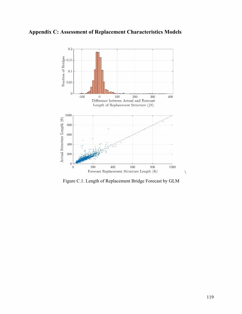
119

Appendix C: Assessment of Replacement Characteristics Models

\

Figure C.1. Length of Replacement Bridge Forecast by GLM

120

Figure C.2. Width of Replacement Bridge Forecast by GLM

121

Figure C.3. Maximum Span Length of Replacement Bridge Forecast by GLM

122

Appendix D: Assessment of Alternative Total Replacement Cost Models

a) b)

c) d)

Figure D.1. Type A GLR Model applied to TIP bridges in Cost Database: a) unit total replacement costs; b) histogram of residual unit total costs; c) total replacement costs; d) histogram of residual total replacement costs

123

a) b)

c) d)

Figure D.2. Type A Decision Tree Model applied to TIP bridges in Cost Database: a) unit total replacement costs; b) histogram of residual unit total costs; c) total replacement costs; d) histogram of residual total replacement costs

124

a) b)

c) d)

Figure D.3. Type B Decision Tree Model applied to TIP bridges in Cost Database: a) unit total replacement costs; b) histogram of residual unit total costs; c) total replacement costs; d) histogram of residual total replacement costs