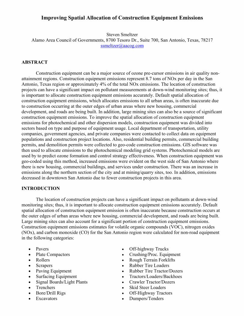
Improving Spatial Allocation of Construction Equipment Emissions

Steven Smeltzer Alamo Area Council of Governments, 8700 Tesoro Dr., Suite 700, San Antonio, Texas, 78217

ssmeltzer@aacog.com

ABSTRACT

Construction equipment can be a major source of ozone pre-cursor emissions in air quality non-attainment regions. Construction equipment emissions represent 8.7 tons of NOx per day in the San Antonio, Texas region or approximately 4% of the total NOx emissions. The location of construction projects can have a significant impact on pollutant measurements at down-wind monitoring sites; thus, it is important to allocate construction equipment emissions accurately. Default spatial allocation of construction equipment emissions, which allocates emissions to all urban areas, is often inaccurate due to construction occurring at the outer edges of urban areas where new housing, commercial development, and roads are being built. In addition, large mining sites can also be a source of significant construction equipment emissions. To improve the spatial allocation of construction equipment emissions for photochemical and other dispersion models, construction equipment was divided into sectors based on type and purpose of equipment usage. Local department of transportation, utility companies, government agencies, and private companies were contacted to collect data on equipment populations and construction project locations. Also, residential building permits, commercial building permits, and demolition permits were collected to geo-code construction emissions. GIS software was then used to allocate emissions to the photochemical modeling grid systems. Photochemical models are used by to predict ozone formation and control strategy effectiveness. When construction equipment was geo-coded using this method, increased emissions were evident on the west side of San Antonio where there is new housing, commercial buildings, and services under construction. There was an increase in emissions along the northern section of the city and at mining/quarry sites, too. In addition, emissions decreased in downtown San Antonio due to fewer construction projects in this area. INTRODUCTION

• • • • • • • • • •

The location of construction projects can have a significant impact on pollutants at down-wind monitoring sites; thus, it is important to allocate construction equipment emissions accurately. Default spatial allocation of construction equipment emission is often inaccurate because construction occurs at the outer edges of urban areas where new housing, commercial development, and roads are being built. Large mining sites can also account for a significant portion of construction equipment emissions. Construction equipment emissions estimates for volatile organic compounds (VOC), nitrogen oxides (NOx), and carbon monoxide (CO) for the San Antonio region were calculated for non-road equipment in the following categories:

Pavers • Off-highway Trucks Plate Compactors • Crushing/Proc. Equipment Rollers • Rough Terrain Forklifts Scrapers • Rubber Tire Loaders Paving Equipment • Rubber Tire Tractor/Dozers Surfacing Equipment • Tractors/Loaders/Backhoes Signal Boards/Light Plants • Crawler Tractor/Dozers Trenchers • Skid Steer Loaders Bore/Drill Rigs • Off-Highway Tractors Excavators • Dumpers/Tenders

• •

Concrete/Industrial Saws • Cranes Cement & Mortar Mixers • Other Construction Equipment

EMISSIONS DEVELOPMENT

• • • • • • • • • • • • •

The methodology used to calculate construction equipment emission estimates for the Alamo Area Council of Government (AACOG) region is based on a methodology developed for the Dallas area, using local data, surveys, and default data from the EPA NONROAD 2005 Emission Inventory Model. The methodology steps are:

1. Conduct surveys and develop surrogate factors to estimate diesel equipment population, usage rates, and equipment characteristics.

2. Update the NONROAD 2005 model input files using local data. 3. Estimate VOC, NOx, and CO annual emissions from construction equipment using the

NONROAD 2005 model. Step 1: Conduct surveys and develop surrogate factors Construction equipment was divided into 25 sectors:

Heavy Highway • Landscaping Businesses Utility • Brick and Stone Businesses Municipal • Trenches Commercial Construction • Concrete Businesses Residential • Skid Steer Loaders City/County Roads • Special Trade Businesses State Transportation Agency • Cranes Scrap Recycling Businesses • RT Forklifts Municipal and County-Op. Eq. • Pipeline Manufacturing • Toyota Bore/Drill Rigs • Quarries Agriculture • Landfills Other

To calculate construction equipment populations in San Antonio, surrogate factors were used to adjust Dallas equipment populations calculated in an Eastern Research Group (ERG) study.1 This methodology was also used in previous studies conducted by ERG for the Capital Area Planning Council of Governments (CAPCOG) and Dallas/Fort Worth regions. To determine surrogate factors for the AACOG region, the Dallas data was divided into industry sectors that facilitated comparisons of industry trends and other data closely related to equipment populations (Table 2-14). The data sources for the surrogate factors are Texas Department of Transportation (TxDOT)2, Texas Water Development Board3, County Business Patterns4, and Census Building permits5. Construction equipment was allocated to the AACOG region by sector using equation 1. Equation (1) EAS = AMAS / AMDS

Where EAS = Equipment allocation to the AACOG region for sector S AMAS = Allocation value for the AACOG region for sector S AMDS = Allocation value for the Dallas region for sector S

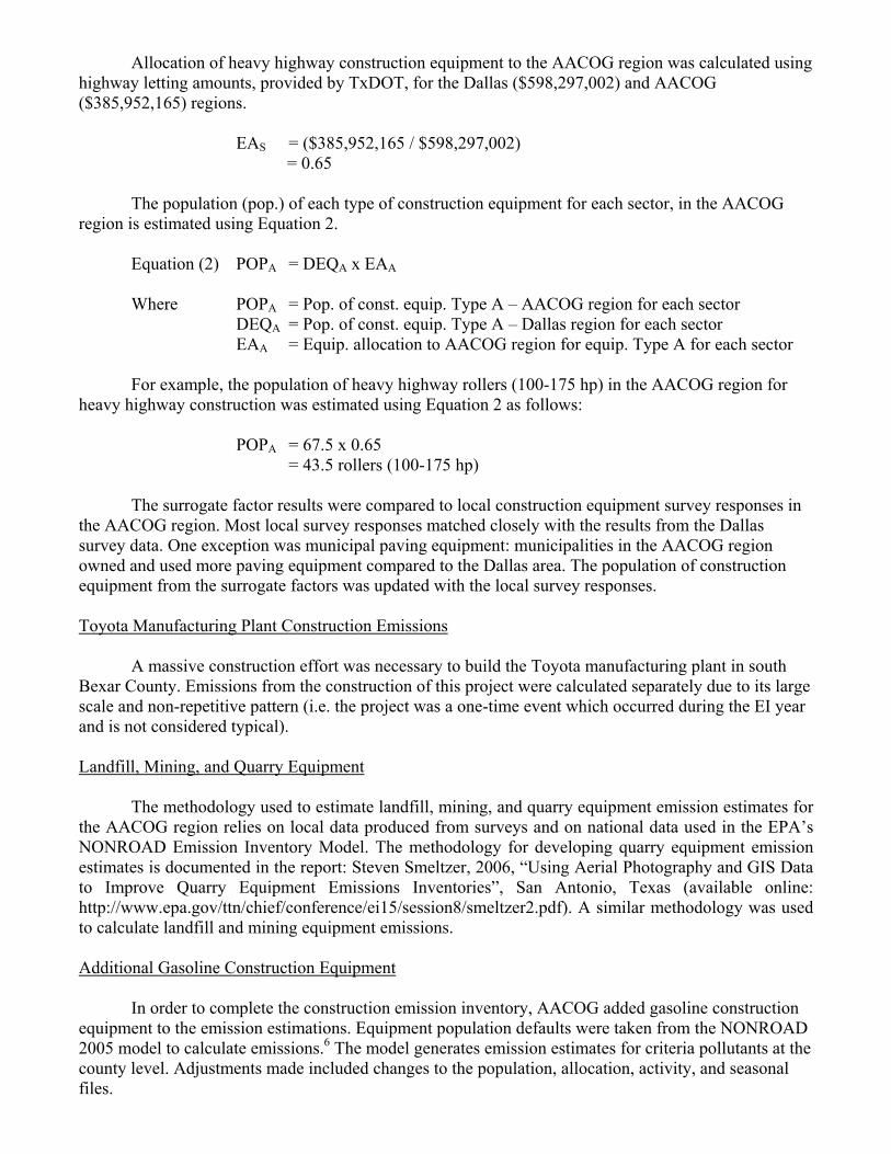
Allocation of heavy highway construction equipment to the AACOG region was calculated using highway letting amounts, provided by TxDOT, for the Dallas ($598,297,002) and AACOG ($385,952,165) regions. EAS = ($385,952,165 / $598,297,002) = 0.65

The population (pop.) of each type of construction equipment for each sector, in the AACOG region is estimated using Equation 2. Equation (2) POPA = DEQA x EAA Where POPA = Pop. of const. equip. Type A – AACOG region for each sector DEQA = Pop. of const. equip. Type A – Dallas region for each sector EAA = Equip. allocation to AACOG region for equip. Type A for each sector For example, the population of heavy highway rollers (100-175 hp) in the AACOG region for heavy highway construction was estimated using Equation 2 as follows:

POPA = 67.5 x 0.65 = 43.5 rollers (100-175 hp)

The surrogate factor results were compared to local construction equipment survey responses in the AACOG region. Most local survey responses matched closely with the results from the Dallas survey data. One exception was municipal paving equipment: municipalities in the AACOG region owned and used more paving equipment compared to the Dallas area. The population of construction equipment from the surrogate factors was updated with the local survey responses. Toyota Manufacturing Plant Construction Emissions

A massive construction effort was necessary to build the Toyota manufacturing plant in south Bexar County. Emissions from the construction of this project were calculated separately due to its large scale and non-repetitive pattern (i.e. the project was a one-time event which occurred during the EI year and is not considered typical). Landfill, Mining, and Quarry Equipment

The methodology used to estimate landfill, mining, and quarry equipment emission estimates for the AACOG region relies on local data produced from surveys and on national data used in the EPA’s NONROAD Emission Inventory Model. The methodology for developing quarry equipment emission estimates is documented in the report: Steven Smeltzer, 2006, “Using Aerial Photography and GIS Data to Improve Quarry Equipment Emissions Inventories”, San Antonio, Texas (available online: http://www.epa.gov/ttn/chief/conference/ei15/session8/smeltzer2.pdf). A similar methodology was used to calculate landfill and mining equipment emissions. Additional Gasoline Construction Equipment

In order to complete the construction emission inventory, AACOG added gasoline construction equipment to the emission estimations. Equipment population defaults were taken from the NONROAD 2005 model to calculate emissions.6 The model generates emission estimates for criteria pollutants at the county level. Adjustments made included changes to the population, allocation, activity, and seasonal files.

Step 2. Update NONROAD 2005 Model Input Files for Local Data Population File Once the equipment population was calculated for each county, the equipment population files were created for each sector in the NONROAD model. Allocation File The construction allocation file for Texas (Tx_const.alo) was updated by replacing values (dollars spent on construction) with zeros for all counties except those in the study area. The value for each county was updated with the surrogate factor for each sector. This allowed the NONROAD model to calculate emissions for the AACOG region as a whole and distribute the emissions to each county appropriately. Activity File

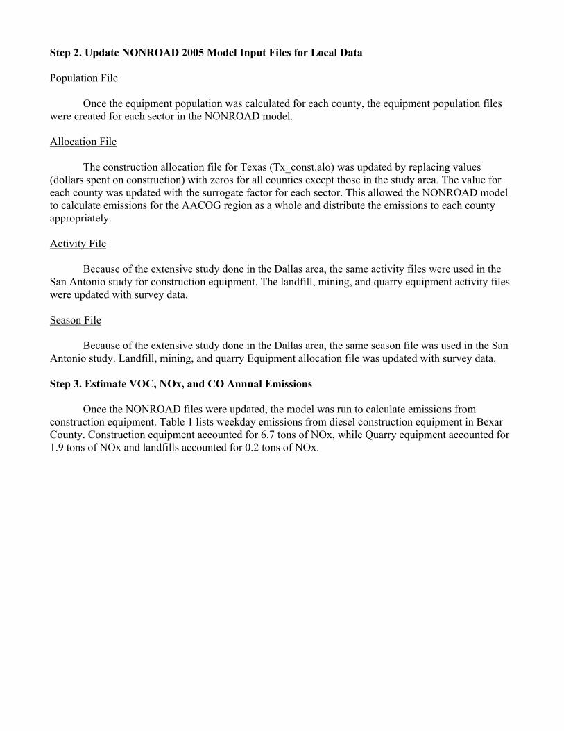
Because of the extensive study done in the Dallas area, the same activity files were used in the San Antonio study for construction equipment. The landfill, mining, and quarry equipment activity files were updated with survey data. Season File Because of the extensive study done in the Dallas area, the same season file was used in the San Antonio study. Landfill, mining, and quarry Equipment allocation file was updated with survey data. Step 3. Estimate VOC, NOx, and CO Annual Emissions Once the NONROAD files were updated, the model was run to calculate emissions from construction equipment. Table 1 lists weekday emissions from diesel construction equipment in Bexar County. Construction equipment accounted for 6.7 tons of NOx, while Quarry equipment accounted for 1.9 tons of NOx and landfills accounted for 0.2 tons of NOx.

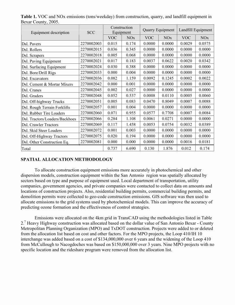
Table 1. VOC and NOx emissions (tons/weekday) from construction, quarry, and landfill equipment in Bexar County, 2005.

Construction Equipment Quarry Equipment Landfill EquipmentEquipment description SCC

VOC NOx VOC NOx VOC NOx Dsl. Pavers 2270002003 0.015 0.174 0.0000 0.0000 0.0029 0.0575 Dsl. Rollers 2270002015 0.036 0.345 0.0000 0.0000 0.0000 0.0000 Dsl. Scrapers 2270002018 0.005 0.068 0.0000 0.0000 0.0000 0.0000 Dsl. Paving Equipment 2270002021 0.017 0.183 0.0037 0.0622 0.0020 0.0342 Dsl. Surfacing Equipment 2270002024 0.030 0.388 0.0000 0.0000 0.0000 0.0000 Dsl. Bore/Drill Rigs 2270002033 0.000 0.004 0.0000 0.0000 0.0000 0.0000 Dsl. Excavators 2270002036 0.082 1.159 0.0092 0.1245 0.0002 0.0022 Dsl. Cement & Mortar Mixers 2270002042 0.000 0.001 0.0000 0.0000 0.0000 0.0000 Dsl. Cranes 2270002045 0.002 0.027 0.0000 0.0000 0.0000 0.0000 Dsl. Graders 2270002048 0.052 0.537 0.0008 0.0110 0.0005 0.0060 Dsl. Off-highway Trucks 2270002051 0.005 0.083 0.0470 0.8049 0.0007 0.0088 Dsl. Rough Terrain Forklifts 2270002057 0.001 0.004 0.0000 0.0000 0.0000 0.0000 Dsl. Rubber Tire Loaders 2270002060 0.071 0.955 0.0577 0.7708 0.0007 0.0084 Dsl. Tractors/Loaders/Backhoes 2270002066 0.284 1.108 0.0061 0.0271 0.0000 0.0000 Dsl. Crawler Tractors 2270002069 0.117 1.458 0.0053 0.0754 0.0032 0.0389 Dsl. Skid Steer Loaders 2270002072 0.001 0.003 0.0000 0.0000 0.0000 0.0000 Dsl. Off-Highway Tractors 2270002075 0.020 0.194 0.0000 0.0000 0.0000 0.0000 Dsl. Other Construction Eq. 2270002081 0.000 0.000 0.0000 0.0000 0.0016 0.0181

Total 0.737 6.690 0.130 1.876 0.012 0.174 SPATIAL ALLOCATION METHODOLOGY To allocate construction equipment emissions more accurately in photochemical and other dispersion models, construction equipment within the San Antonio region was spatially allocated by sectors based on type and purpose of equipment used. Local department of transportation, utility companies, government agencies, and private companies were contacted to collect data on amounts and locations of construction projects. Also, residential building permits, commercial building permits, and demolition permits were collected to geo-code construction emissions. GIS software was then used to allocate emissions to the grid systems used by photochemical models. This can improve the accuracy of predicting ozone formation and the effectiveness of control strategies.

Emissions were allocated on the 4km grid in TransCAD using the methodologies listed in Table 2.7 Heavy Highway construction was allocated based on the dollar value of San Antonio Bexar - County Metropolitan Planning Organization (MPO) and TxDOT construction. Projects were added to or deleted from the allocation list based on cost and other factors. For the MPO projects, the Loop 410/IH 10 interchange was added based on a cost of $134,000,000 over 6 years and the widening of the Loop 410 from McCullough to Nacogdoches was based on $150,000,000 over 3 years. Nine MPO projects with no specific location and the rideshare program were removed from the allocation list.

Table 2. Spatial allocation surrogates used to allocate construction equipment emissions. Sector Spatial Allocation Methodology Heavy Highway TxDOT and MPO Construction Dollar Value Utility CPS, BexarMet, and SAWS Construction Dollar Value Commercial Construction COSA and Bexar County Com. Building and Demolition Permits Residential COSA and Bexar County Residential Building Permits City/County Roads COSA and Bexar County Road Dollar Value TxDOT TxDOT and MPO Construction Dollar Value Scrap Recycling Scrap and waste Materials Employment Landscaping EPA Default Brick and Stone Related construction materials Employment Concrete Block, brick, other, and ready-mix Employment Special Trade COSA and Bexar County Commercial Building Permits Municipal/County-Op. Eq. COSA and Bexar County Road Dollar Value Manufacturing Manufacturing Employees (only companies > 4 employees) Agriculture Crop Location (Cotton, Small Grains, Hay, Corn, Sorghum, Peanuts) Toyota Location of Toyota Landfills Location of Landfills Quarries Location of Quarries Other Sectors Total Construction Dollar Value

Utility construction emissions were geo-coded based on the dollar value of San Antonio water

system (SAWS), Bexar Metropolitan Water District (BexarMet), and City Public Service (CPS) 2005 construction projects. SAWS permits were culled to remove projects with final acceptance dates before March 31, 2005, construction start dates after Nov. 1, 2005, current permit dates after Nov. 1, 2005, expired permits (2 permit), and unknown addresses (9 permits). For CPS construction, projects with close dates before March 31, 2005, gas lines with no addresses, and small projects with no addresses (6 projects) were removed. Also, transmission line projects were removed because these projects are very expensive, but typically do not require the extensive use of heavy construction equipment.

Commercial construction allocation was based on the number of Bexar County and City of San Antonio commercial building/demolition permits. The voided permits, stop work permits, partial construction, portable buildings, and “master plan only not to be built” (2) permits were removed from the city of San Antonio commercial building permit database before using the database for allocation purposes. Partial demolition permits were also removed. For Bexar County, all 2005 commercial sewage permits were used. Number of city of San Antonio and Bexar County residential building permits were used to geo-code residential construction. Voided permits, stop work permits, partial construction, house move, and “without an address: master plan” (31) permits were removed from the city of San Antonio database. For Bexar County, all 2005 residential sewage permits were used to geo-code residential construction. Figures 1 to 10 show the location of construction projects used to allocate emissions for each sector.

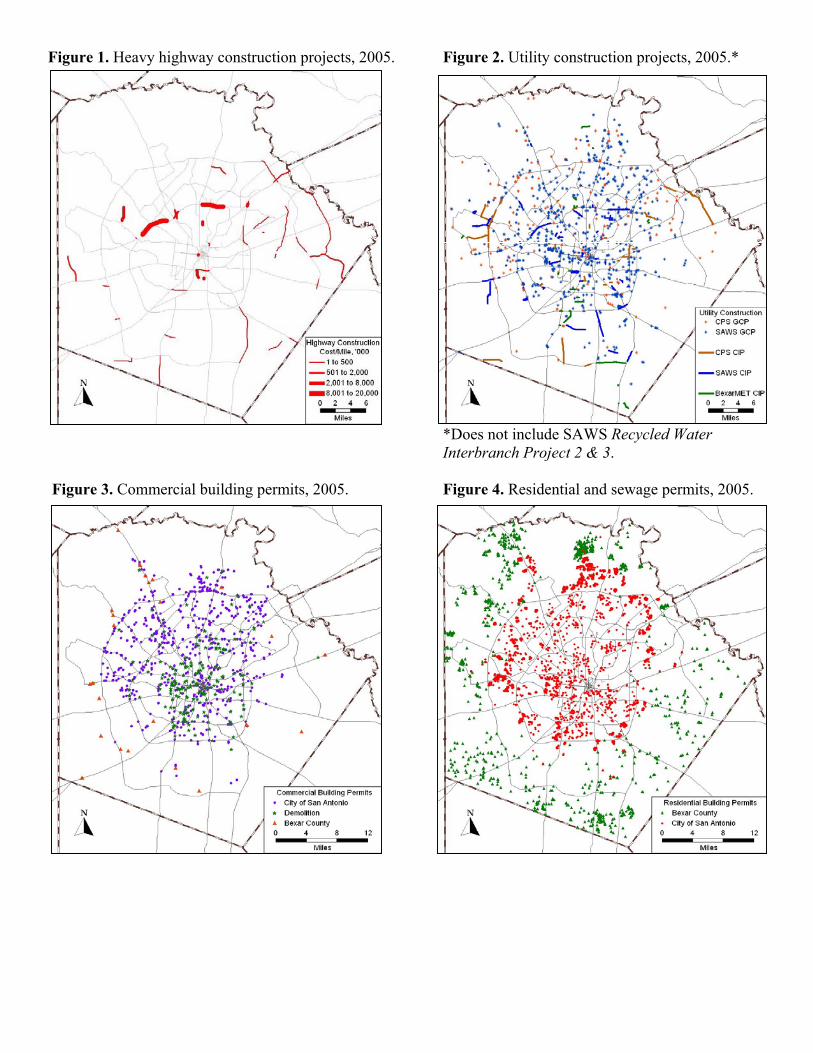
Figure 1. Heavy highway construction projects, 2005. Figure 2. Utility construction projects, 2005.*

*Does not include SAWS Recycled Water Interbranch Project 2 & 3.

Figure 3. Commercial building permits, 2005. Figure 4. Residential and sewage permits, 2005.

Figure 5. City and County Road Construction Figure 6. Scrap and Waste Materials Projects, 2005. Employment, 2005.

Figure 7. Brick and stone employment, 2005. Figure 8. Concrete employment, 2005.

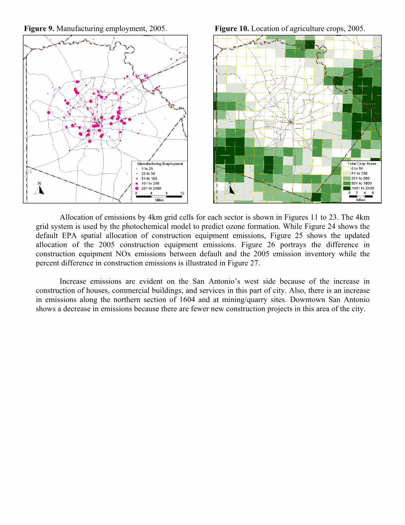
Figure 9. Manufacturing employment, 2005. Figure 10. Location of agriculture crops, 2005.

Allocation of emissions by 4km grid cells for each sector is shown in Figures 11 to 23. The 4km grid system is used by the photochemical model to predict ozone formation. While Figure 24 shows the default EPA spatial allocation of construction equipment emissions, Figure 25 shows the updated allocation of the 2005 construction equipment emissions. Figure 26 portrays the difference in construction equipment NOx emissions between default and the 2005 emission inventory while the percent difference in construction emissions is illustrated in Figure 27.

Increase emissions are evident on the San Antonio’s west side because of the increase in construction of houses, commercial buildings, and services in this part of city. Also, there is an increase in emissions along the northern section of 1604 and at mining/quarry sites. Downtown San Antonio shows a decrease in emissions because there are fewer new construction projects in this area of the city.

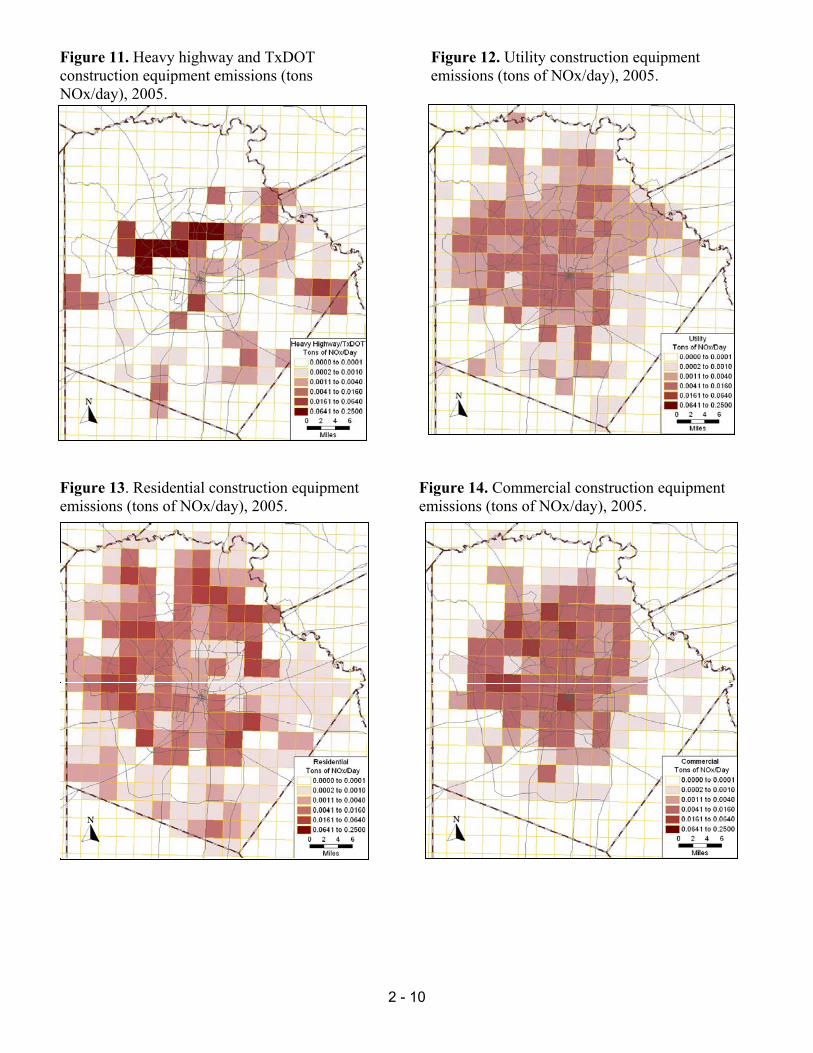
Figure 11. Heavy highway and TxDOT Figure 12. Utility construction equipment construction equipment emissions (tons emissions (tons of NOx/day), 2005. NOx/day), 2005.

Figure 13. Residential construction equipment Figure 14. Commercial construction equipment emissions (tons of NOx/day), 2005. emissions (tons of NOx/day), 2005.

2 - 10

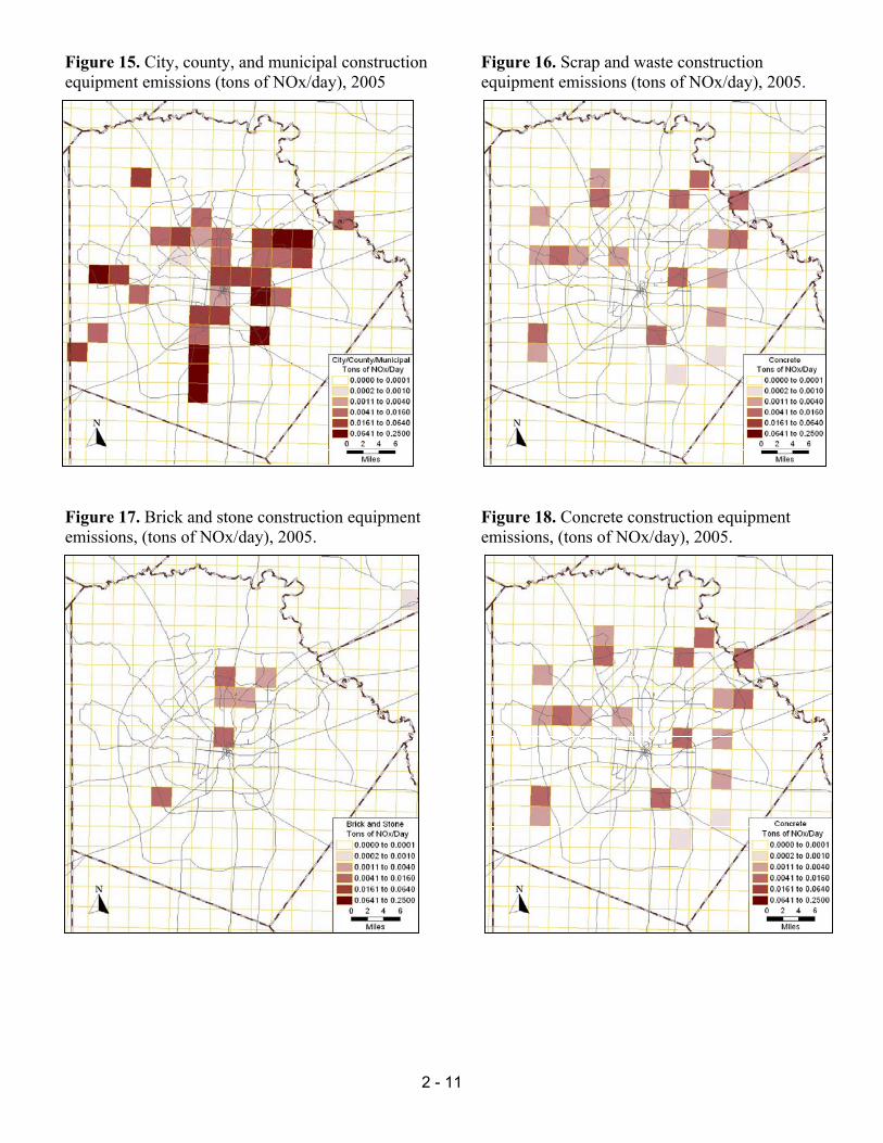
Figure 15. City, county, and municipal construction Figure 16. Scrap and waste construction equipment emissions (tons of NOx/day), 2005 equipment emissions (tons of NOx/day), 2005.

Figure 17. Brick and stone construction equipment Figure 18. Concrete construction equipment emissions, (tons of NOx/day), 2005. emissions, (tons of NOx/day), 2005.

2 - 11

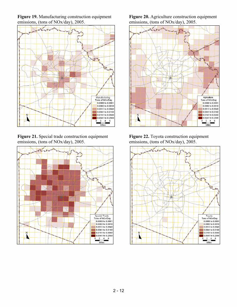
Figure 19. Manufacturing construction equipment Figure 20. Agriculture construction equipment emissions, (tons of NOx/day), 2005. emissions, (tons of NOx/day), 2005.

Figure 21. Special trade construction equipment Figure 22. Toyota construction equipment emissions, (tons of NOx/day), 2005. emissions, (tons of NOx/day), 2005.

2 - 12

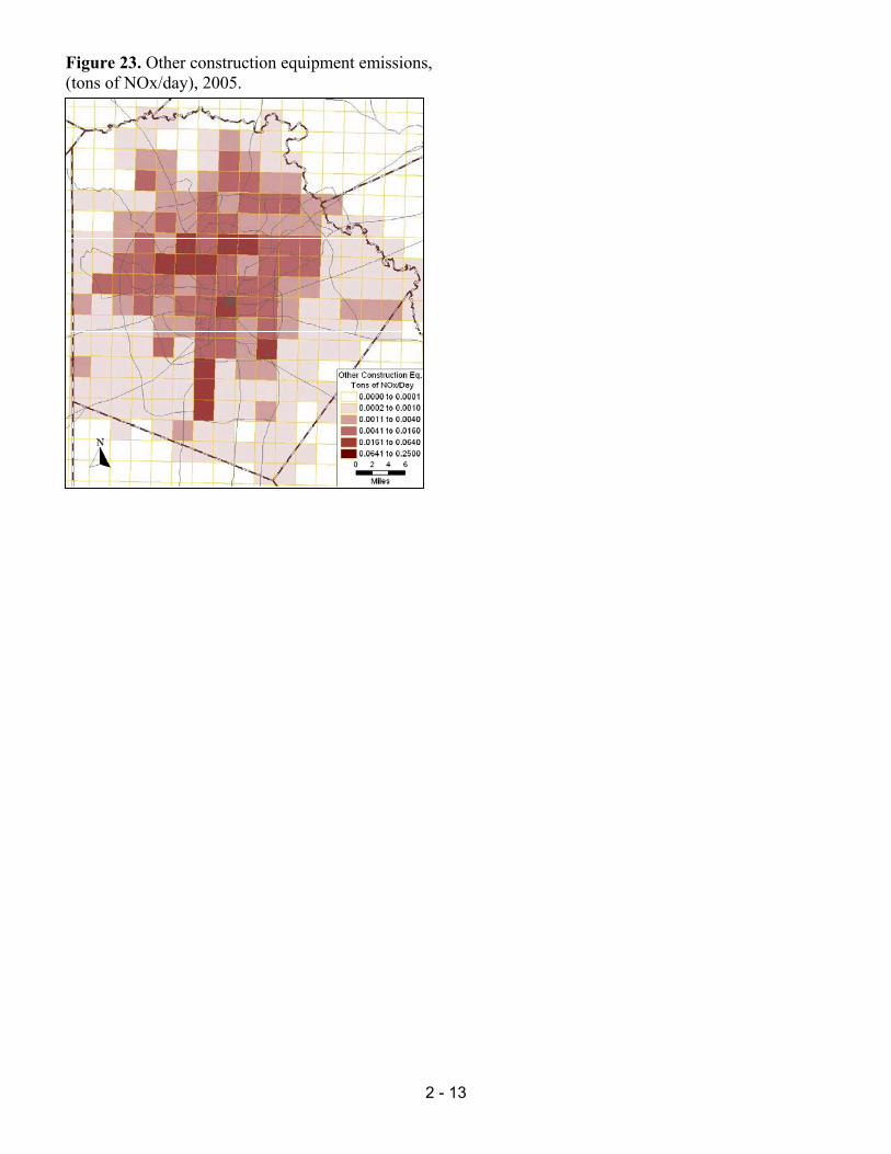
Figure 23. Other construction equipment emissions, (tons of NOx/day), 2005.

2 - 13

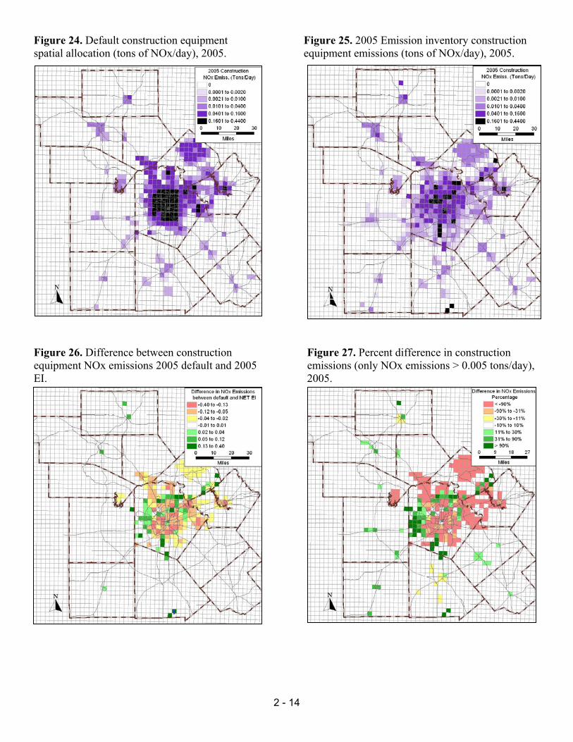
Figure 24. Default construction equipment Figure 25. 2005 Emission inventory construction spatial allocation (tons of NOx/day), 2005. equipment emissions (tons of NOx/day), 2005.

Figure 26. Difference between construction Figure 27. Percent difference in construction equipment NOx emissions 2005 default and 2005 emissions (only NOx emissions > 0.005 tons/day), EI. 2005.

2 - 14

PHOTOCHEMICAL MODEL UPDATE FOR NEW SPATIAL ALLOCATION

Four South Texas near non-attainment areas (Austin, Corpus Christi, San Antonio, and Victoria), along with the Texas Commission on Environmental Quality (TCEQ), sponsored the development of a Comprehensive Air Quality Model with Extensions (CAMx) photochemical model simulating the high-ozone episode that occurred between September 13th and 20th, 1999.8 Development of the 1999 simulation and projections provide a representation of future air quality conditions so that pollution control measures could be modeled and analyzed for their effectiveness. The model was updated with the latest emission inventory for 2005 to increase the accuracy of the model when determining the effectiveness of control strategies.

When the updated spatial allocated construction equipment emissions were put into the photochemical model instead of the default EPA spatial allocation methodology, there was a significant impact on ozone formation. For both runs, total construction equipment emissions and daily allocation were constant. Table 3 lists the results for selected Continuous Air Monitoring Stations (CAMS) in the San Antonio region. The greatest increase in predicted ozone, 0.44 ppb 8-hour ozone average, occurred at CAMS 678 near downtown San Antonio on Sept. 15th, while the largest decrease, -0.16 ppb, occurred at CAMS 23 on Sept. 16. The predicted 8-hour ozone values were between –0.11 and 0.36 at the controlling monitor in the San Antonio region, CAMS 58. There was no significant ozone difference on Sept. 18 and 19th because these modeling days are on the weekends with lower construction equipment usage. Table 3. Impact of the updated spatial allocated construction equipment on ozone formation at selected CAMS station.

Change in 8-hour ozone average, 2005 (ppb.) Wednesday Thursday Friday Saturday Sunday Monday CAMS Station

Sept. 15 Sept. 16 Sept. 17 Sept. 18 Sept. 19 Sept. 20 CAMS 58 0.09 -0.11 -0.03 -0.01 -0.01 0.36 CAMS 23 0.18 -0.16 -0.05 -0.01 -0.01 0.35 CAMS 59 0.06 -0.01 0.01 0.00 0.01 0.30 CAMS 678 0.44 -0.01 0.39 0.02 0.01 0.40 Figures 28 to 33 show the predicted ozone difference between the default spatial allocation and the updated spatial allocation for each day of the modeling episode. The greatest difference is observed on Sept. 20, although there are significant differences in predicted ozone on Sept. 15 and Sept. 16.

2 - 15

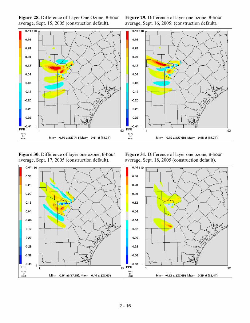
Figure 28. Difference of Layer One Ozone, 8-hour Figure 29. Difference of layer one ozone, 8-hour average, Sept. 15, 2005 (construction default). average, Sept. 16, 2005: (construction default).

Figure 30. Difference of layer one ozone, 8-hour Figure 31. Difference of layer one ozone, 8-hour average, Sept. 17, 2005 (construction default). average, Sept. 18, 2005 (construction default).

2 - 16

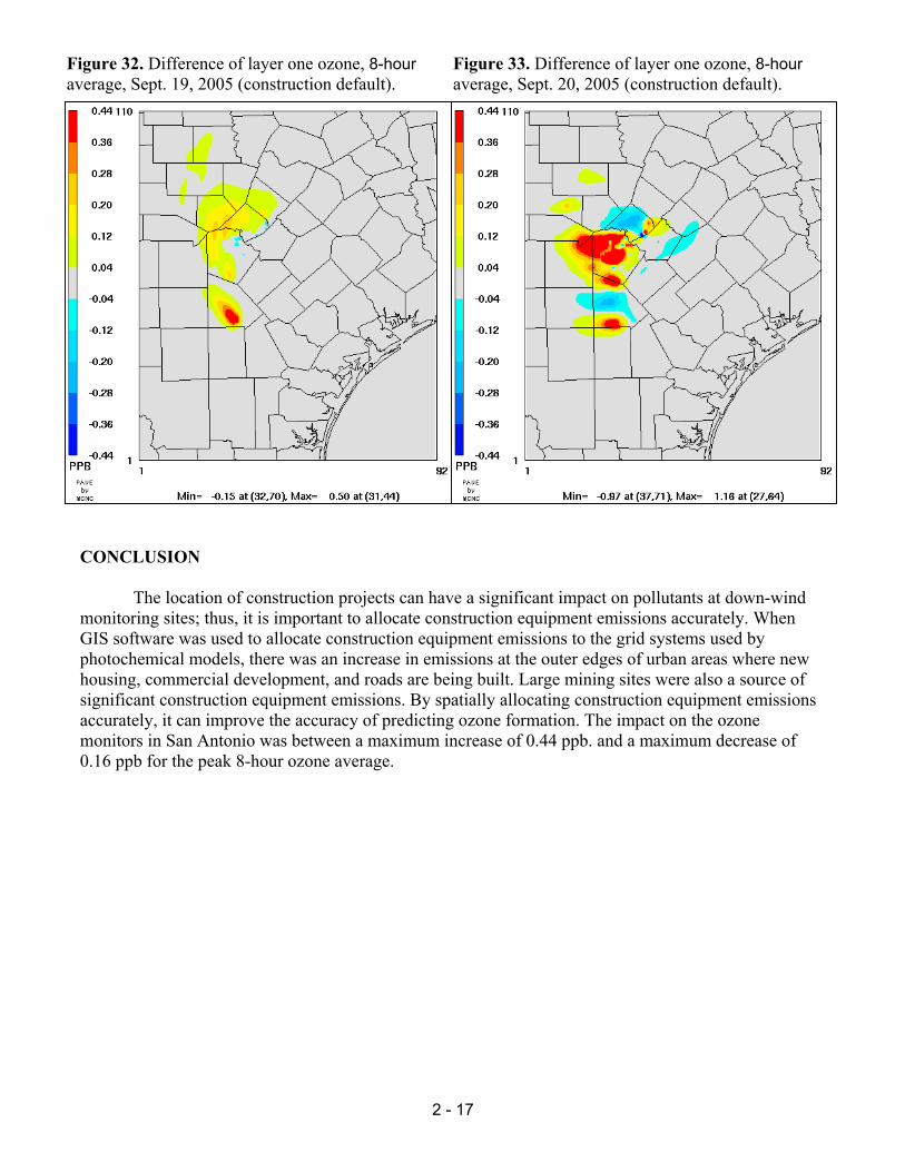
Figure 32. Difference of layer one ozone, 8-hour Figure 33. Difference of layer one ozone, 8-hour average, Sept. 19, 2005 (construction default). average, Sept. 20, 2005 (construction default).

CONCLUSION

The location of construction projects can have a significant impact on pollutants at down-wind monitoring sites; thus, it is important to allocate construction equipment emissions accurately. When GIS software was used to allocate construction equipment emissions to the grid systems used by photochemical models, there was an increase in emissions at the outer edges of urban areas where new housing, commercial development, and roads are being built. Large mining sites were also a source of significant construction equipment emissions. By spatially allocating construction equipment emissions accurately, it can improve the accuracy of predicting ozone formation. The impact on the ozone monitors in San Antonio was between a maximum increase of 0.44 ppb. and a maximum decrease of 0.16 ppb for the peak 8-hour ozone average.

2 - 17

REFERENCES 1 Eastern Research Group, Inc. August 31, 2005. Ozone Science and Air Modeling Research Project H43T163: Diesel Construction Equipment Activity and Emissions Estimates for the Dallas/Ft. Worth Region. Austin, TX 78731. 2 Texas Department of Transportation, Aug. 15, 2005. Letting Schedule for San Antonio and Dallas District (FY 2005). Finance Division, Austin, Texas. Available online: http://www.dot.state.tx.us/insdtdot/orgchart/cmd/cserve/let/2005/letsat.htm and http://www.dot.state.tx.us/insdtdot/orgchart/cmd/cserve/let/2005/letdal.htm 3 Texas Water Development Board, April 2006. 2006 Regional Water Plan: County Population Projections for 2000 - 2060. Austin, TX. Available online: http://www.twdb.state.tx.us/data/popwaterdemand/2003Projections/Population%20Projections/STATE_REGION/County_Pop.htm

4 U.S. Census Bureau, July 14, 2006, County Business Patterns, 2004. Available online: http://www.census.gov/epcd/cbp/view/cbpview.html. 5 U.S. Census Bureau, 2006. Building Permits. Available online: http://www.census.gov/const/www/permitsindex.html

6 U.S. Environmental Protection Agency, Feb. 10, 2006. Final Nonroad 2005 Model. Ann Arbor, MI. Available online: http://www.epa.gov/otaq/nonrdmdl.htm 7 Caliper Corporation, TRANSCAD: Transportation GIS Software Version 4.7, 2005, Newton MA 8 ENVIRON. August 6, 2002. Development of a Joint CAMx Photochemical Modeling Database for the Four Southern Texas Near Non-Attainment Areas, Final Report. Novato, California.

2 - 18

2 - 19

KEY WORDS Construction Equipment Emission Inventory GIS NONROAD model Spatial Allocation Highway Construction