Improving Value at RiskCalculations by Using Copulas

and Non-Gaussian Margins

�

Dr J. R.

New College

University of Oxford

A thesis submitted in partial fulfillment of the requirements for the MSc in

Mathematical Finance

November 30, 2002

MSc in Mathematical Finance

New College

OXFORD UNIVERSITY

Authenticity Statement

I hereby declare that this dissertation is my own work and confirm its authenticity.

Name Dr J. R.

Address .........

Signed

Date

Abstract

Value at risk (VaR) is of central importance in modern financial risk management.

Of the various methods that exist to compute the VaR, the most popular are historical

simulation, the variance-covariance method and Monte Carlo (MC) simulation. While

historical simulation is not based on particular assumptions as to the behaviour of

the risk factors, the two other methods assume some kind of multinormal distribution

of the risk factors. Therefore the dependence structure between different risk factors

is described by the covariance or correlation between these factors.

It is shown in [1, 2] that the concept of correlation entails several pitfalls. As a

consequence, copulas are proposed to describe the dependence between n variables

with arbitrary marginal distributions. A copula is a function C : [0, 1]n → [0, 1]

with certain special properties [3], so that the joint distribution can be written as

IP(R1 ≤ r1, . . . , Rn ≤ rn) = C (F1(r1), . . . , Fn(rn)). F1, . . . , Fn denote the cumulative

probability functions of the n variables. In general, a copula C depends on one

or more parameters p1, . . . , pk that determine the dependence between the variables

r1, . . . , rn. In this sense, these parameters assume the role of correlations.

The second pitfall that arises from the multinormal distribution ansatz is the fat

tail problem of the margins [4, 5]. One way of taking extreme values better into

account is to assume that the risk factors obey Student distribution patterns instead

of Gaussian patterns.

In this thesis we investigate two risk factors only. We model each risk factor

independently using a Student distribution and describe their dependence by both

the Frank copula [6] and the Gumbel-Hougaard copula [7]. We present algorithms

to estimate the parameters of the margins and the copulas and to generate pseudo

random numbers due to a copula dependence.

Making use of historical data spanning a period of nineteen years, we compute the

VaR using a copula-modified MC algorithm. To see the advantage of this method, we

compare our results with VaR results obtained from the three standard methods men-

tioned at the beginning. Based on backtesting results, we find that the copula method

is more reliable than both traditional MC simulation and the variance-covariance

method and about as good as historical simulation.

To Christiane and Maximilian

Acknowledgements

I would like to express my gratitude towards my actual employer d-fine

GmbH and my former employer Arthur Andersen Wirtschaftsprufungs-

gesellschaft, Steuerberatungsgesellschaft mbH for financing this course

and giving me the necessary time off work. In particular I am very grateful

to Dr Hans-Peter Deutsch, head of d-fine GmbH and former head of the

Financial and Commodity Risk Consulting Group of Arthur Andersen in

Germany, who has given me the opportunity to participate in this course.

In addition, I would like to thank Dr Jeff Dewynne, Dr Sam Howison and

all other lecturers for plenty of interesting lectures during the modules.

Of course, many thanks also go to Ms Tiffany Fliss, Ms Anna Turner and

Ms Roz Sainty for organising the whole course so well and reliably.

Furthermore, I am very grateful to Dr Thomas Siegl who brought my

attention to the mathematical theory of copulas and who acted as a proof-

reader of this thesis.

My special word of thanks is dedicated to my beloved wife Christiane for

all her patience during the many weekends that I had to spend on writing

this thesis and on other MSc-related work.

Contents

1 Introduction 1

2 Traditional Monte Carlo Simulation of the Value at Risk 5

3 Basic Features of Copulas 9

3.1 Definition of a Copula . . . . . . . . . . . . . . . . . . . . . . . . . . 9

3.2 Examples of Copulas . . . . . . . . . . . . . . . . . . . . . . . . . . . 10

3.2.1 The Product Copula . . . . . . . . . . . . . . . . . . . . . . . 10

3.2.2 Bounding Copulas . . . . . . . . . . . . . . . . . . . . . . . . 11

3.2.3 The Frank Copula . . . . . . . . . . . . . . . . . . . . . . . . 11

3.2.4 The Gumbel-Hougaard Copula . . . . . . . . . . . . . . . . . 12

3.2.5 The Gaussian Copula . . . . . . . . . . . . . . . . . . . . . . . 13

3.3 Sklar’s Theorem and Further Important Properties of Copulas . . . . 14

3.4 Copulas and Random Variables . . . . . . . . . . . . . . . . . . . . . 17

4 Generation of Pseudo Random Numbers Using Copulas 19

4.1 The General Method . . . . . . . . . . . . . . . . . . . . . . . . . . . 19

4.2 t-Distributed Pseudo Random Numbers with a Copula Dependence

Structure . . . . . . . . . . . . . . . . . . . . . . . . . . . . . . . . . 20

5 Numerical Results 24

6 Summary and Conclusions 38

A Generation of Pseudo Random Numbers 41

A.1 Transformation of Variables . . . . . . . . . . . . . . . . . . . . . . . 41

A.2 The Box-Muller Method . . . . . . . . . . . . . . . . . . . . . . . . . 42

A.3 Pseudo Random Numbers According to the Multinormal Distribution 42

i

B The t-Distribution 45

B.1 The Density Function . . . . . . . . . . . . . . . . . . . . . . . . . . . 45

B.2 The Distribution Function . . . . . . . . . . . . . . . . . . . . . . . . 47

C The Maximum Likelihood Method 48

C.1 Theoretical Background . . . . . . . . . . . . . . . . . . . . . . . . . 48

C.2 Estimation of the Degrees of Freedom of the t-Distribution Using the

ML Method . . . . . . . . . . . . . . . . . . . . . . . . . . . . . . . . 50

C.3 ML Estimation of the Copula Parameter . . . . . . . . . . . . . . . . 52

Bibliography 54

ii

Chapter 1

Introduction

In modern financial risk management, one fundamental quantity of interest is value

at risk (VaR). It denotes the amount by which a portfolio of financial assets might

fall at the most with a given probability during a particular time horizon. For the

sake of simplification we will only consider time horizons of one day’s length in this

thesis. This covers portfolios that include assets that can be sold in one day. The

discussions would have to be modified slightly if we were interested in longer time

horizons.

Typical choices of the probabilities that are connected with VaRs are confidence

levels of 90%, 95% and 99%, respectively. If a risk manager is free to choose,1 the

particular value he might select will depend on weighing the reliability that he ex-

pects from the VaR prediction against the amount a VaR should have. Using a high

confidence level, e.g., 99%, will result in a higher absolute VaR compared with a 90%

VaR. If the risk manager compares the predicted VaRs of the portfolio with the real

losses of the following business days over a sufficiently long period of time, he will

observe that about 1% of the real losses exceeds the calculated 99% VaRs, assuming

the method the VaR predictions are based on were reliable. However, if he had chosen

a confidence level of 90%, backtesting of the data would deliver underestimated losses

of 10%.

In statistics, the gap between the confidence level and 100% is called the quantile

and usually denoted by the Greek letter α. Once the risk manager has chosen a

confidence level 1 − α, it is vital that he can trust the predicted VaRs, i.e., that

he can be sure that the fraction of underestimated losses is in fact very close to α.

Otherwise, the larger the difference between the fraction of underestimated losses

1In some countries the confidence level to choose is prescribed by law. For example, in Germanya confidence level of 99% is required for internal models [8].

1

and α, the less useful the VaR is for managing the risk of the portfolio. Therefore, a

reliable method is needed to compute the VaR.

In literature, several methods to calculate the VaR are known. The most popular

are

• historical simulation,

• the variance-covariance method and

• Monte Carlo (MC) simulation.

As it is not within the scope of this thesis, we will not explain the first two methods.

Excellent descriptions of these and of what we will term “traditional” Monte Carlo

can be found in [4, 9].

We next present general information on how to compute the VaR of a portfolio

using Monte Carlo simulation. The value of the portfolio at present time t will be

denoted by Vt. Let us assume that Vt depends on n risk factors which might be

(relative) interest rates, foreign exchange (FX) rates, share prices, etc. Then a Monte

Carlo computation of the VaR would consist of the following steps:

1. Choose the level of confidence 1 − α to which the VaR refers.

2. Simulate the evolution of the risk factors from time t to time t+1 by generating

n-tuples of pseudo random numbers (PRNs) with appropriate marginal distri-

butions and an appropriate joint distribution that describe the behaviour of the

risk factors. The number m of these n-tuples has to be large enough (typically

m = O(1000)) to obtain sufficient statistics in step 5.

3. Calculate the m different values of the portfolio at time t + 1 using the values

of the simulated n-tuples of the risk factors. Let us denote these values by

Vt+1,1, Vt+1,2, . . . , Vt+1,m.

4. Calculate the simulated profits and losses, i.e., the differences between the sim-

ulated future portfolio values and the present portfolio value, ∆Vi = Vt+1,i − Vt

for i = 1, . . . ,m.

5. Ignore the fraction of the α worst changes ∆Vi. The minimum of the remain-

ing ∆Vi s is then the VaR of the portfolio at time t. It will be denoted by

VaR(α, t, t + 1).

2

As soon as the time evolves from t to t+1, the real value of the (unchanged) port-

folio changes from Vt to Vt+1. With this data at hand, one can backtest VaR(α, t, t+1)

by comparing it with ∆V = Vt+1 − Vt.

It is obvious that the central point in the above algorithm is step two, the genera-

tion of the PRNs according to the appropriate distributions. Therefore the following

questions have to be answered:

Question 1 What are the appropriate marginal distributions of the risk factors under

consideration?

Question 2 What is the appropriate joint distribution of the risk factors under con-

sideration?

Question 3 Is it possible to simulate PRNs using these marginal distributions and

this joint distribution?

Finding answers to the above questions for two risk factors is the main objective of

this work. For this purpose, the thesis is organised as follows:

In the following chapter, the traditional Monte Carlo method is presented. In Chap-

ter 3, copulas are defined. Examples of these functions are given and the basic prop-

erties are summarised. Copulas can be used to describe the dependence structure

between two or more variables. In this sense they replace the concept of covari-

ance or correlation that is usually used to describe the dependence between variables.

Chapter 4 is concerned with the simultaneous generation of pairs of PRNs whose

dependence structure is determined by a copula.

After the theoretical introduction we present in Chapter 5 numerical results of a

VaR Monte Carlo simulation based on copulas. The portfolio for which the VaR is

calculated is affected by two risk factors only. The first risk factor we have used is the

foreign exchange (FX) rate GBP/DEM.2 The second risk factor in our calculations

is one of the FX rates USD/DEM, JPY/DEM, CHF/DEM and FRF/DEM. The

FX rates that we have used are daily data ranging from 02/01/1980 to 30/12/19983

[10]. For the marginal distributions of the two risk factors we have used the Student

distribution. To test the quality of the copula MC simulation, we backtest our data

2The abbreviations that we use for the currencies are the corresponding ISO codes: CHF (Swissfranc), DEM (German mark), FRF (French franc), GBP (British pound sterling), JPY (Japaneseyen), USD (United States dollar)

3With the start of European Monetary Union by 01/01/1999, the German mark and the Frenchfranc ceased to exist as independent currencies. Therefore we have chosen 30/12/1998 as the finalday of our investigation.

3

and compare the results with numerical VaR predictions obtained from the traditional

MC simulation, from the variance-covariance method and from historical simulation.

Finally, we give a summary and our conclusions in Chapter 6.

The appendix at the end of this thesis contains some well known statistical tools

that we used to obtain our numerical results. It starts with a short overview of

the generation of pseudo random numbers, followed by a section on the Student

distribution and ends with a description of the maximum likelihood method.

4

Chapter 2

Traditional Monte CarloSimulation of the Value at Risk

In this chapter we recall the joint simulation of risk factors which is used with most

Monte Carlo based methods used for computing the VaR. In other words, we want

to explain the second step on page 2 in more detail.

As the algorithm we will present next is the one that is most often used in practice,

we will refer to it as the “traditional method”. This is to distinguish it from the new

method which will be presented in Chapter 4 and which we will call the “copula

method”.

Let us briefly recapitulate the content of the second step mentioned above. It

states that we have to generate n-tuples of PRNs with appropriate marginal distri-

butions and an appropriate joint distribution that describe the behaviour of the risk

factors. If we only take FX rates as risk factors into account, the traditional ansatz

to achieve these PRNs consists of the following steps:

1. Collect historical data of the n FX rates, i.e., n time series spanning N + 1

business days. We denote these data by xi,0, xi,1, . . . , xi,N for i = 1, . . . , n,

where today’s data are given by the xi,N ’s.

A typical choice for N + 1 is, for example, N + 1 = 250.

2. Assuming xi,j 6= 0, compute the relative changes in the data:

ri,j =xi,j − xi,j−1

xi,j−1

for i = 1, . . . n and j = 1, . . . , N . (2.1)

For each i = 1, . . . , n, the ri,1, . . . , ri,N will be considered as elements belonging

to a random variable ri.

5

3. The next step is to make an assumption as to the marginal distributions f1, . . . ,

fn of the random variables r1, . . . , rn.

As the r1, . . . , rn originally come from FX rates, the assumption usually made in

finance at this point is that the fi s are given by normal distributions N (µi, σ2i ),

fi(ri) =1

√

2πσ2i

exp

{

−(ri − µi)2

2σ2i

}

(2.2)

for i = 1, . . . , n. In (2.2), µi and σ2i denote the mean and the variance of ri,

µi = IE(ri) , σ2i = IE((ri − µi)

2) . (2.3)

4. In general, the parameters of the marginal distributions are unknown. We have

to determine estimators for these parameters from the historical data.

In the case of normal distributions, this task is easy4 because the parameters

of the normal distributions are the mean and the variance of the distribution.

Their estimators can be calculated as

µi =1

N

N∑

j=1

ri,j and (2.4)

σ2i =

1

N − 1

N∑

j=1

(ri,j − µi)2 (2.5)

for i = 1, . . . , n.

Note that the mean and the variance of an arbitrary distribution, provided that

they are well defined, can also be estimated by (2.4) and (2.5). This is essantially

a consequence of the law of large numbers. In addition, these estimators are

unbiased and consistent [11].

5. As stated above, we want to generate n-tuples of PRNs according to a joint

distribution. Therefore we have to make a further assumption, i.e., an assump-

tion that describes the dependence structure of the random variables. As the

marginal distributions have already been chosen, we are, of course, not com-

pletely free to choose the joint distribution. If f(~r) denotes the joint distribu-

tion, we have to ensure that the following condition is true for each i = 1, . . . , n:

fi(ri) =

∫

∞

−∞

dr1 . . .

∫

∞

−∞

dri−1

∫

∞

−∞

dri+1 . . .

∫

∞

−∞

drn f(~r) . (2.6)

4“Easy” in the sense that we can calculate the estimators directly from the historical data withoutthe use of any kind of numerical algorithm (see Appendix C).

6

Let us return to our traditional Monte Carlo simulation. Here we assume at

this point a multinormal distribution,

f(~r) =1

√

(2π)n det Cexp

{

−1

2(~r − ~µ) t C−1 (~r − ~µ)

}

, (2.7)

where

~r =

r1...rn

, ~µ =

µ1...

µn

, (2.8)

and C denotes the covariance matrix,

C =

σ21 c1,2 c1,3 · · · c1,n

c1,2 σ22 c2,3 · · · c2,n

c1,3 c2,3 σ23

. . ....

......

. . . . . . cn−1,n

c1,n c2,n · · · cn−1,n σ2n

, (2.9)

where ci,j is the covariance between ri and rj,

ci,j = IE ((ri − µi)(rj − µj)) . (2.10)

For the sake of completeness, we introduce the correlations at this point. They

are given by

ρi,j ≡ci,j

σiσj

if σi, σj 6= 0 . (2.11)

One can easily show that the function f given in (2.7) fulfils condition (2.6).

However, we would like to emphasise that the normal marginal distributions

do not imply a joint distribution of the multinormal kind. This point is a

direct consequence from Sklar’s theorem (see page 17). This is essential for

understanding the copula ansatz. Furthermore, it was explained in [1, 2] that a

dependence structure, which is, like the multinormal distribution, described by

correlation, entails several pitfalls.

6. This step of the algorithm consists of a determination of the covariances (2.10).

In a similar way as the means and variances in step 4, they can be estimated as

ci,j =1

N − 1

N∑

k=1

(ri,k − µi) (rj,k − µj) . (2.12)

7

7. As we have chosen the marginal distributions (step 3) and a joint distribution

(step 5) and have estimated its parameters (steps 4 and 6) we now have all tools

at hand to generate the desired n-tuples of PRNs. Because this is a standard

technical procedure, we present it in detail in Appendix A.3. The relevant steps

required are given on page 43, steps (a) and (b) for n dimensions, and steps (a)

and (b) for two dimensions only. Let us therefore assume at this point that we

have generated n-tuples of PRNs. We denote these numbers by

~rk =

rk1...rkn

(2.13)

where k = 1, . . . ,m, and m is the number of Monte Carlo iterations.

8. The previous step provided us with m independent n-tuples of PRNs. However,

these numbers are related to the relative changes in the data (see step 2).

Therefore we finally have to compute the absolute values of the simulated risk

factors. From (2.1) and (2.13) the m simulated values of the n risk factors at

time step N + 1 are given by

xki,N+1 = xi,N (1 + rk

i ) (2.14)

where i = 1, . . . , n and k = 1, . . . ,m.

So far, we have presented the traditional method of generating PRNs, assuming

that the marginal distributions of the relative risk factors are given by normal dis-

tributions (see step 3, equation (2.2)) and the joint distribution of the relative risk

factors is given by a multinormal distribution (see step 5, equation (2.7)). As al-

ready outlined in the introduction, we want to replace step 3 by the assumption that

each margin obeys a Student distribution. Then we want to replace step 5 by the

assumption that a copula can be used to describe the dependence structure between

the margins. To be able to understand the copula method, we present the basic fea-

tures of copulas in the following chapter. Chapter 4 then shows how to replace the

steps 3–7 from the algorithm above.

8

Chapter 3

Basic Features of Copulas

In this chapter we summarise the basic definitions that are necessary to understand

the concept of copulas. We then present the most important properties of copulas

that are needed to understand the usage of copulas in finance.

We will follow the notation used in [3]. As it would exceed the scope of this thesis,

we do not present the proofs of the theorems cited. At this point we again refer to the

excellent textbook by Nelson [3]. Furthermore, we will restrict ourselves to copulas

of two dimensions only. The generalisation to n dimensions can also be found in [3].

3.1 Definition of a Copula

Definition 1 A two-dimensional copula is a function C : [0, 1] × [0, 1] → [0, 1] with

the following properties:5

1. For every u, v ∈ [0, 1]:

C(u, 0) = C(0, v) = 0 . (3.1)

2. For every u, v ∈ [0, 1]:

C(u, 1) = u and C(1, v) = v . (3.2)

3. For every u1, u2, v1, v2 ∈ [0, 1] where u1 ≤ u2 and v1 ≤ v2:

C(u2, v2) − C(u2, v1) − C(u1, v2) + C(u1, v1) ≥ 0 . (3.3)

5In mathematical literature, the letter C is commonly used in conjunction with continuous func-tions. As we will show in Theorem 1 (see page 14), a copula is even uniformly continuous on itsdomain.

9

0

0.2

0.4

0.6

0.8

1

0 0.2 0.4 0.6 0.8 10

0.2

0.4

0.6

0.8

10

0.2

0.4

0.6

0.8

1

v

u

Π(u,v)

Figure 3.1: The product copula.

Below we will use the shorthand notation copula for C. As the usage of the name

copula for the function C is not obvious from Definition 1, it will be explained at the

end of Section 3.3.

A function that fulfils property 1 is also said to be grounded. Property 3 is the

two-dimensional analogue of a non-decreasing one-dimensional function. A function

with this feature is therefore called 2-increasing.

3.2 Examples of Copulas

This section starts with three examples of copulas that have a very simple structure.

These copulas are very important as they represent some characteristic features. Then

we introduce three families of copulas. A copula family is defined by a copula function

that includes an additional free parameter.

3.2.1 The Product Copula

The first example we want to consider is the product copula. It is given by the function

Π(u, v) ≡ uv (3.4)

which is also shown in Figure 3.1. As stated in Theorem 4 (see page 18) the special

10

0 0.2 0.4 0.6 0.8 100.20.40.60.810

0.2

0.4

0.6

0.8

1

vu

M(u,v)

0

0.2

0.4

0.6

0.8

1

0 0.2 0.4 0.6 0.8 100.20.40.60.810

0.2

0.4

0.6

0.8

1

vu

W(u,v)

Figure 3.2: The Frechet-Hoeffding upper (left) and lower (right) bounds.

importance of the product copula goes back to the description of independent random

variables.

3.2.2 Bounding Copulas

The copula defined by

M(u, v) ≡ min(u, v) (3.5)

is called the Frechet-Hoeffding upper bound. It can be shown that for any given copula

C one has C(u, v) ≤ M(u, v) for all u, v ∈ [0, 1].

By contrast, the Frechet-Hoeffding lower bound is defined by

W (u, v) ≡ max(u + v − 1, 0) . (3.6)

For W one finds W (u, v) ≤ C(u, v) for any given copula C and all u, v ∈ [0, 1]. Both

M and W are presented in Figure 3.2.

3.2.3 The Frank Copula

The Frank copula [6] is our first example of a 1-parameter copula family. It is given

by

CFrank(u, v) ≡

−1θln

[

1 +(e−θu

−1)(e−θv−1)

e−θ−1

]

∀ θ ∈ ]−∞,∞[\{0}uv for θ = 0

. (3.7)

11

0 0.2 0.4 0.6 0.8 100.20.40.60.810

0.2

0.4

0.6

0.8

1

vu

θ = 3.1

CFrank

(u,v)

0

0.2

0.4

0.6

0.8

1

0 0.2 0.4 0.6 0.8 100.20.40.60.810

0.2

0.4

0.6

0.8

1

vu

θ = −3.1

CFrank

(u,v)

Figure 3.3: The Frank copula for positive (left) and negative (right) values of thecopula parameter θ.

The influence of the copula parameter θ on the dependence structure between the two

variables u and v is shown in Figure 3.3.6 As one might already assume by comparing

Figure 3.3 with Figures 3.1 and 3.2, the Frank copula obeys the following properties

CFrank(u, v)θ→∞−→ M(u, v) , (3.8)

CFrank(u, v)θ→−∞−→ W (u, v) , (3.9)

CFrank(u, v)|θ=0 = Π(u, v) . (3.10)

A copula family that contains M , W and Π is called comprehensive.

3.2.4 The Gumbel-Hougaard Copula

The next copula we want to consider is the Gumbel-Hougaard copula [7]. It is given

by the function

CGH(u, v) ≡ exp{

−[

(− ln u)θ + (− ln v)θ]1/θ

}

. (3.11)

The parameter θ may take all values in the interval [1,∞[. In Figure 3.4 we present

the graph of the Gumbel-Hougaard copula for θ = 1.4.7

6The value θ = 3.1 as used in Figure 3.3 was not chosen arbitrarily. It describes the dependencestructure of the relative FX rates USD/DEM vs. GBP/DEM, obtained from historical data of theperiod 02/01/1980 to 30/12/1998. See Chapter 5 for details.

7As in the case of the Frank copula (see footnote 6), the value θ = 1.4 as used in Figure 3.4describes the dependence structure of the relative FX rates USD/DEM vs. GBP/DEM under theassumption of a Gumbel-Hougaard copula.

12

0

0.2

0.4

0.6

0.8

1

0 0.2 0.4 0.6 0.8 10

0.2

0.4

0.6

0.8

10

0.2

0.4

0.6

0.8

1

v

u

θ = 1.4

CGH

(u,v)

Figure 3.4: The Gumbel-Hougaard copula for θ = 1.4.

A discussion in [1, 2] shows that CGH is suitable to describe positive depen-

dence structures, i.e., the Gumbel-Hougaard copula “is consistent with bivariate ex-

treme value theory and could be used to model the limiting dependence structure of

component-wise maxima of bivariate random samples” [2]. We will come back to this

point later in this thesis (page 27).

Like relations (3.8) and (3.10) one finds for the Gumbel-Hougaard copula

CGH(u, v)θ→∞−→ M(u, v) , (3.12)

CGH(u, v)|θ=1 = Π(u, v) . (3.13)

However, a relation equivalent to (3.9) does not exist for the Gumbel-Hougaard cop-

ula, i.e., the Gumbel-Hougaard copula is not comprehensive.

3.2.5 The Gaussian Copula

The last copula that we want to introduce is the Gaussian or normal copula [2],

CGauss(u, v) ≡∫ Φ−1

1 (u)

−∞

dr1

∫ Φ−12 (v)

−∞

dr2 f(r1, r2) . (3.14)

In (3.14), f denotes the bivariate normal density function, i.e., the function defined by

(2.7) for n = 2. The function Φ1 in (3.14) refers to the one-dimensional, cumulative

13

normal density function,

Φ1(r1) =

∫ r1

−∞

dr′1 f1(r′

1) , (3.15)

where f1 is given by equation (2.2). For Φ2 an analogous expression holds.

If the covariance between r1 and r2 is zero, the Gaussian copula becomes

CGauss(u, v) =

∫ Φ−11 (u)

−∞

dr1 f1(r1)

∫ Φ−12 (v)

−∞

dr2 f2(r2)

= u v (3.16)

= Π(u, v) if c1,2 = 0 .

As we will see in Section 3.4, result (3.16) is a direct consequence of Theorem 4.8

As Φ1(r1), Φ2(r2) ∈ [0, 1], we can replace u, v in (3.14) by Φ1(r1), Φ2(r2). If we

consider r1, r2 in a probabilistic sense, i.e., r1 and r2 being values of two random

variables R1 and R2, we obtain from (3.14)

CGauss(Φ1(r1), Φ2(r2)) = IP(R1 ≤ r1, R2 ≤ r2) . (3.17)

In other words, CGauss(Φ1(r1), Φ2(r2)) is the binormal cumulative probability function.

3.3 Sklar’s Theorem and Further Important Prop-

erties of Copulas

In this section we focus on the properties of copulas. The theorem we will present

next establishes the continuity of copulas via a Lipschitz condition on [0, 1] × [0, 1]:

Theorem 1 Let C be a copula. Then for every u1, u2, v1, v2 ∈ [0, 1]:

|C(u2, v2) − C(u1, v1)| ≤ |u2 − u1| + |v2 − v1| . (3.18)

From (3.18) it follows that every copula C is uniformly continuous on its domain.

A further important property of copulas concerns the partial derivatives of a

copula with respect to its variables:

Theorem 2 Let C be a copula. For every u ∈ [0, 1], the partial derivative ∂ C/∂ v

exists for almost all9 v ∈ [0, 1]. For such u and v one has

0 ≤ ∂

∂ vC(u, v) ≤ 1 . (3.19)

8See also footnote 16 on page 27.9The expression “almost all” is used in the sense of the Lebesgue measure.

14

The analogous statement is true for the partial derivative ∂ C/∂ u. Consequently, the

functions

u → Cv(u) ≡ ∂ C(u, v)/∂ v and v → Cu(v) ≡ ∂ C(u, v)/∂ u (3.20)

are well defined on [0,1].

In addition, Cv and Cu are non-decreasing almost everywhere on [0,1].

To give some examples of this theorem, we consider the partial derivatives of the

Frank copula and the Gumbel-Hougaard copula with respect to u. Let us start with

the Frank copula (3.7). As the discussion would be trivially for θ = 0, we consider in

the following the case θ ∈ ]−∞,∞[\{0} only. From definition (3.7) we have

CFrank,u(v) =e−θu

(

e−θv − 1)

e−θ − 1 + (e−θu − 1) (e−θv − 1)∀ θ ∈ ]−∞,∞[\{0} . (3.21)

Obviously, CFrank,u is defined for all v ∈ [0, 1]. CFrank,u in particular is a strictly

increasing function of v. The inverse function can be calculated analytically and is

given by

C−1Frank,u(y) = −1

θln

[

1 + y(

eθ(u−1) − 1)

1 + y (eθu − 1)

]

∀ θ ∈ ]−∞,∞[\{0} . (3.22)

The second example of Theorem 2 deals with the Gumbel-Hougaard copula (3.11).

Its partial derivative with respect to u is given by

CGH,u(v) = exp{

−[

(− ln u)θ + (− ln v)θ]1/θ

}

×[

(− ln u)θ + (− ln v)θ]

−θ−1

θ(− ln u)θ−1

u.

(3.23)

In Figure 3.5, CGH,u is shown for u = 0.1, 0.2, . . . , 0.9 and θ = 2.0. Note that for

u ∈ ]0, 1[ and for all θ ∈ IR where θ ≥ 1, CGH,u is a strictly increasing function of

v. Therefore the inverse function C−1GH,u is well defined. However, as one might guess

from (3.23), C−1GH,u cannot be calculated analytically so that some kind of numerical

algorithm has to be used for this task.

As CFrank and CGH are both symmetric in u and v, the partial derivatives of CFrank

and CGH with respect to v exhibit identical behaviours for the same set of parameters.

We now turn to the central theorem in the theory of copulas, Sklar’s theorem [12].

To be able to understand it, we recall some terms known from statistics.

Definition 2 A distribution function is a function F : IR → [0, 1] with the following

properties:

15

0 0.25 0.5 0.75 10

0.25

0.5

0.75

1

v

CGH,u

(v)

u = 0.1 →

← u = 0.9

Figure 3.5: The partial derivative CGH,u of the Gumbel-Hougaard copula for u =0.1, 0.2, . . . , 0.9 and θ = 2.0.

1. F is non-decreasing.

2. F (−∞) = 0 and F (+∞) = 1.

For example, if f is a probability density function, then the cumulative probability

function

F (x) =

∫ x

−∞

dt f(t) (3.24)

is a distribution function.

Definition 3 A joint distribution function is a function H : IR× IR → [0, 1] with the

following properties:

1. H is 2-increasing.

2. For every x1, x2 ∈ IR: H(x1,−∞) = H(−∞, x2) = 0 and H(+∞, +∞) = 1.

It is shown in [3] that H has margins F1 and F2 that are given by F1(x1) ≡ H(x1, +∞)

and F2(x2) ≡ H(+∞, x2). Furthermore, F1 and F2 themselves are distribution func-

tions.

In Section 3.2.5 we have already given an example of a two-dimensional function

satisfying the properties of Definition 3. If one considers CGauss as given in (3.17) as

16

a function of r1 and r2, it can be seen as the joint distribution function belonging to

the binormal distribution.

We now have all the definitions that we need for Sklar’s theorem.

Theorem 3 (Sklar’s theorem) Let H be a joint distribution function with margins

F1 and F2. Then there exists a copula C where

H(x1, x2) = C(F1(x1), F2(x2)) (3.25)

for every x1, x2 ∈ IR. If F1 and F2 are continuous, then C is unique. Otherwise, C is

uniquely determined on Range F1 × Range F2. On the other hand, if C is a copula

and F1 and F2 are distribution functions, then the function H defined by (3.25) is a

joint distribution function with margins F1 and F2.

With Sklar’s theorem in mind the use of the name “copula” becomes obvious. It was

chosen by Sklar to describe [13] “a function that links a multidimensional distribution

to its one-dimensional margins” and appeared in mathematical literature for the first

time in [12]. Usually, the term “copula” is used in grammar to describe an expression

that links a subject and a predicate. The origin of the word is Latin.

3.4 Copulas and Random Variables

So far we have considered functions of one or two variables. We now turn our attention

to random variables. As already used at the end of Section 3.2.5, we will denote

random variables by capital letters and their values by lower case letters. In the

definition of a random variable and its distribution function we again follow [3]:

Definition 4 A random variable R is a real valued measurable function on a prob-

ability space whose distribution is described by a probability density function f(r),

where the domain of f is the range of R.

Note that it is not stated whether or not the probability function f is known.

Definition 5 The distribution function of a random variable R is a function F that

assigns all r ∈ IR a probability F (r) = IP(R ≤ r). In addition, the joint distribution

function of two random variables R1, R2 is a function H that assigns all r1, r2 ∈ IR a

probability H(r1, r2) = IP(R1 ≤ r1, R2 ≤ r2).

17

We want to emphasise that (joint) distribution functions in the sense of Defi-

nition 5 are also (joint) distribution functions in the sense of Definitions 2 and 3.

Therefore equation (3.25) from Sklar’s theorem can be written as

H(r1, r2) = C(F1(r1), F2(r2)) = IP(R1 ≤ r1, R2 ≤ r2) . (3.26)

Before we can present the next important property of copulas we first have to

introduce the term of independent variables:

Definition 6 Two random variables R1 and R2 are independent if and only if the

product of their distribution functions F1 and F2 equals their joint distribution func-

tion H,

H(r1, r2) = F1(r1) F2(r2) for all r1, r2 ∈ IR . (3.27)

In Section 3.2.1 we have already mentioned the product copula Π (see equation

(3.4)). The next theorem clarifies the importance of this copula.

Theorem 4 Let R1 and R2 be random variables with continuous distribution func-

tions F1 and F2 and joint distribution function H. From Sklar’s theorem we know

that there exists a unique copula CR1R2 where

IP(R1 ≤ r1, R2 ≤ r2) = H(r1, r2) = CR1R2(F1(r1), F2(r2)) . (3.28)

Then R1 and R2 are independent if and only if CR1R2 = Π.

We will end this section with a statement on the behaviour of copulas under

strictly monotone transformations of random variables.

Theorem 5 Let R1 and R2 be random variables with continuous distribution func-

tions and with copula CR1R2 . If α1 and α2 are strictly increasing functions on

Range R1 and Range R2, then Cα1(R1) α2(R2) = CR1R2 . In other words: CR1R2 is

invariant under strictly increasing transformations of R1 and R2.

18

Chapter 4

Generation of Pseudo RandomNumbers Using Copulas

In the last chapter we presented the definition of copulas and their most important

properties, especially Sklar’s theorem. We are thus ready to return to the Monte

Carlo simulation of the value at risk. The strategy, as already outlined at the end

of Chapter 2, is to give a general guide on how to generate pairs of t-distributed

pseudo random numbers whose dependence structure is given by a copula.10 As the

numerical results presented in the following chapter assume either a Frank copula

or a Gumbel-Hougaard copula, we will focus our attention on these copulas where

necessary.

4.1 The General Method

Let us assume that the copula C we are interested in is known, i.e., all parameters of

the copula are known. The task is then to generate pairs (u, v) of observations of in

[0, 1]× [0, 1] uniformly distributed random variables U and V whose joint distribution

function is C. To reach this goal we will use the method of conditional distributions.

Let cu denote the conditional distribution function for the random variable V at a

given value u of U ,

cu(v) ≡ IP(V ≤ v, U = u) . (4.1)

From (3.26) and (4.1) and using the notation introduced in (3.20) we obtain11

cu(v) = lim∆u→0

C(u + ∆u, v) − C(u, v)

∆u=

∂

∂uC(u, v) = Cu(v) . (4.2)

10The incorporation of the copula dependence structure will follow very closely the instructionsgiven in [3].

11Note that if Funiform denotes the distribution function of a random variable U which is uniformlydistributed in [0, 1], we have Funiform(u) = u.

19

From Theorem 2 we know that cu(v) is non-decreasing and exists for almost all

v ∈ [0, 1].

For the sake of simplicity, we assume from now on that cu is strictly increasing

and exists for all v ∈ [0, 1]. As discussed in Section 3.3, this is at least true for

the Frank and the Gumbel-Hougaard families of copulas. If these conditions are not

fulfilled, we have to replace the term “inverse” in the remaining part of this section

by “quasi-inverse” (see [3] again for details).

With result (4.2) at hand we can now use the method of variable transformation,

which is described in Appendix A.1, to generate the desired pair (u, v) of PRNs. The

algorithm consists of the following two steps:

• Generate two independent uniform PRNs u,w ∈ [0, 1]. Here u is already the

first number we are looking for.

• Compute the inverse function of cu. In general, it will depend on the parameters

of the copula and on u, which can be seen, in this context, as an additional

parameter of cu. Set v = c−1u (w) to obtain the second PRN.

It may happen that the inverse function cannot be calculated analytically. In this

case one can try to use a numerical algorithm to determine v. For example, this

situation occurs when the Gumbel-Hougaard copula is used, as already mentioned in

Section 3.3.

4.2 t-Distributed Pseudo Random Numbers with

a Copula Dependence Structure

In this section we present a detailed example of the application of the copula method

in the calculation of the value at risk. We refer to the algorithm presented in Chapter 2

and will use the same notation.

As stated at the end of Chapter 2, we want to replace steps 3–7 of the traditional

algorithm. On a more abstract level, these steps have the following content:

Step 3: For each margin, choose a proper distribution function.

Step 4: Determine the parameters of the distribution functions of the margins from

historical data.

Step 5: Choose a joint distribution function that describes the dependence structure

of the problem under consideration.

20

Step 6: Determine the parameter(s) of the joint distribution function from historical

data.

Step 7: Generate n-tuples (or simply pairs) of PRNs according to the distributions

of the margins with respect to the joint distribution.

Let us first turn to step 3 as mentioned on page 6. We have chosen the normal

distribution function (2.2) to describe each margin. We replace this assumption by

the following more general12 one:

Step 3 (copula method): The probability density functions that describe the risk

factors are generalised t-distributions (see Appendix B.1 for details),

fi(ri) =Γ

(

ki+12

)

Γ(

ki

2

)

Γ(

12

)√ki − 2 σi

(

1 +(ri − µi)

2

(ki − 2) σ2i

)

−ki+1

2

for i = 1, 2 . (4.3)

The degrees of freedom k1 and k2 are both restricted to numbers that are greater

or equal to three. This is to ensure that the variances of f1 and f2 are well

defined. To keep the cost of numerical computations low, we restrict ourselves

to the values ki = 3, 4, 5, . . . for i = 1, 2.

Step 4 of the original algorithm deals with the estimation of the parameters of the

marginal distributions. It will be modified to

Step 4 (copula method): The parameters µi and σ2i are the mean and the variance

of the marginal distribution (4.3) for each i = 1, 2 (see Appendix B.1 for details).

Therefore µi and σi can be calculated by using equations (2.4) and (2.5), as

already mentioned in step 4 of the original algorithm.

Using µi and σi we can consider each fi as a function of one free parameter ki

for i = 1, 2. To estimate k1 and k2 we use the maximum likelihood method as

described in Appendix C.2.

We now come to step 5. Here we have chosen the multinormal distribution function

to describe the dependence structure. As the numerical results that we will present

in the next chapter are based on two risk factors only, we will only consider the

case n = 2 below. We thus have to replace a binormal distribution function by an

alternative dependence structure.

With Sklar’s theorem in mind (see equation (3.26)), we now make the following

assumption:

12As the t-distribution converges in the limit k → ∞ to the normal distribution (see Appendix B),one can consider the t-distribution as a generalisation of the normal distribution.

21

Step 5 (copula method): The joint distribution function of the two risk factors is

given by a 1-parameter copula family,

C(F1(r1), F2(r2)) = IP(R1 ≤ r1, R2 ≤ r2) . (4.4)

The Fi are the distribution functions of the t-distributions (4.3). They are given

in Appendix B.2, equations (B.16)-(B.18). The copula parameter will be called

θ below.

When comparing (4.4) with expression (3.17) it becomes obvious that what we call

the copula method actually involves two replacements. The Gaussian copula in the

traditional method is replaced by an alternative copula, for example, the Frank cop-

ula or the Gumbel-Hougaard copula. In addition, the Gaussian distributions of the

margins are replaced by t-distributions.

Next we consider step 6 of the original algorithm. For two risk factors only, it shows

how to estimate the covariance or the correlation between these factors (see equation

(2.12)). Note that this is the only parameter that results from the assumption that

the joint distribution is of the binormal kind. From (3.17) and (4.4) it is obvious that

the role of the correlation ρ ≡ ρ1,2 in the traditional method is assumed by the copula

parameter θ in the copula method. Therefore, step 6 is modified as follows:

Step 6 (copula method): To estimate θ we again use the maximum likelihood

method, see Appendix C.3. From the cumulative probability (4.4) we derive

a probability density by calculating the partial derivative of C with respect to

both parameters,

f(r1, r2) ≡ ∂2

∂r1 ∂r2

C(F1(r1), F2(r2))

=∂2

∂u ∂vC(u, v)

∣

∣

∣

∣

u=F1(r1),v=F2(r2)

f1(r1) f2(r2) . (4.5)

For the Frank copula, we can compute the partial derivative in (4.5) using

equation (3.21). It follows that

∂2

∂u ∂vCFrank(u, v) =

e−θue−θv(

1 − e−θ)

θ

[e−θ − 1 + (e−θu − 1) (e−θv − 1)]2. (4.6)

For the Gumbel-Hougaard copula, we obtain from (3.23)

∂2

∂u ∂vCGH(u, v) =

(− ln u)θ−1

u

(− ln v)θ−1

v×

e−Σ1/θ (

Σ−2(θ−1)/θ + (θ − 1)Σ−(2θ−1)/θ)

(4.7)

22

where Σ ≡ (− ln u)θ + (− ln v)θ. With equations (4.5)-(4.7) at hand the likeli-

hood function can be computed,

L(θ) = L((r1,1, r2,1), . . . , (r1,N , r2,N) ; θ) =N∏

j=1

f(r1,j, r2,j) . (4.8)

The N pairs (r1,j, r2,j) are again the relative changes of the historical data (see

equation (2.1) in Chapter 2).

From the numerical maximisation of L(θ) we finally obtain θ. A detailed dis-

cussion of this point is contained in Appendix C.3.

Let us now come to step 7 of the original algorithm. Instead of creating pairs of

correlated PRNs that belong to binormal distributed random variables, we now have

to generate PRNs that obey the copula dependence structure that was chosen in (4.4)

with the parameter θ and the marginal distributions that were selected in (4.3). Using

the results from Section 4.1, step 7 can now be reformulated:

Step 7 (copula method): First, generate two independent, in [0, 1] uniformly dis-

tributed PRNs u,w. Compute v = C−1u (w). For the Frank copula, C−1

Frank,u

is given by equation (3.22). In the case of the Gumbel-Hougaard copula,

C−1GH,u has to be computed numerically from equation (3.23). Finally deter-

mine r1 = F−11 (u) and r2 = F−1

2 (v) to obtain one pair (r1, r2) of PRN with the

desired copula dependence structure.

Let us end this chapter with two remarks on the last step. As already discussed

in Section 3.3, the determination of C−1GH,u(w) is generally possible from a numerical

point of view. Secondly, we also computed F−11 (u) and F−1

2 (v) numerically to obtain

the results which are presented in following chapter.

23

Chapter 5

Numerical Results

As already mentioned in the previous chapters, we considered just two risk factors in

our numerical simulations. These factors are the FX rate GBP/DEM and one out of

the FX rates USD/DEM, JPY/DEM, CHF/DEM and FRF/DEM.

For the copula method, we were using both the Frank copula (3.7) and the

Gumbel-Hougaard copula (3.11). Furthermore, for each copula we tested margins

that were assumed to be normally distributed (2.2) and t-distributed (4.3).

To see how copulas can improve the calculation of the value at risk and to demon-

strate the benefits it is not necessary to use a complicated portfolio. The VaR results

that we will discuss below are therefore based on a simple linear portfolio that contains

both a long position and a short position. Its value is given by

V = ∆Curr × Curr − 1000 × GBP , (5.1)

where the long position of the portfolio is given by Curr ∈ {USD, JPY, CHF, FRF}.As we are interested in the value of V given in DEM, one can say that the portfolio

contains the risk factors directly.

The data on which our investigation is based are the historical daily FX rates

ranging from 02/01/1980 to 30/12/1998 [10]. To make the results of the four portfolios

comparable, we have computed the means of the five FX rates under consideration

during this period. The results are listed in Table 5.1.13 With these results at hand,

we have chosen the quantities ∆Curr in a way that the average DEM value of the

long position equals the average DEM value of the short position for each of the

four portfolios. We therefore have ∆USD = 1640, ∆JPY = 253323, ∆CHF = 2708 and

∆FRF = 10024.

13As we need the results that are shown in Table 5.1 for the determination of the portfolio weightsonly, we do not present any errors of the values.

24

currency mean of DEM value

1 GBP 3.19395

1 USD 1.94745

100 JPY 1.26082

1 CHF 1.17945

10 FRF 3.18610

Table 5.1: Means of the DEM values of the currencies under investigation for theperiod 02/01/1980 to 30/12/1998.

Each time interval on which a VaR computation was based consisted of 250 busi-

ness days. Using the notation given in step 1 on page 5, we used N + 1 = 250 to

obtain our results. This corresponds to a time horizon of one banking year. Because

of this moving time window, the first date for which we were able to calculate a VaR

is 02/01/1981.

Let us now start our comparison of the traditional method vs. the copula method of

calculating the value at risk. First, we want to take a look at the different parameters

of the underlying joint distributions, i.e., the correlation ρ = ρ1,2 of the binormal

distribution, the parameter θFrank of the Frank copula and the parameter θGH of

the Gumbel-Hougaard copula. The behaviour of these parameters is presented in

Figure 5.1,14 where we show ρ, θFrank and θGH, obtained from the relative GBP/DEM

rates vs. the relative CHF/DEM rates, against time. As already mentioned in the

previous chapters, the theoretical values that these parameters may take are ρ ∈[−1, +1], θFrank ∈ ]−∞,∞[ and θGH ∈ [1,∞[.

A comparison of ρ and θFrank shows that the directions of both curves behave in

a similar manner on a qualitative level. However, even though it is most often the

case, an increase or decrease in one of the parameters does not necessarily result in an

increase or decrease in the other. Particularly there is no unique relation between ρ

and θFrank. This can also be seen from the right part of Figure 5.2. There we present

the same data as shown in Figure 5.1. The difference between both figures is that

θGH and θFrank are now plotted against ρ.

14In Figures 5.1 and 5.2 we only show the copula parameters θFrank and θGH for t-distributedmargins. The behaviour of the copula parameters does not change on a qualitative level if we areusing normally distributed margins. Therefore we omit a discussion of the corresponding values ofkGBP and kCHF at this point (see also Figure 5.5).

25

1982 1984 1986 1988 1990 1992 1994 1996 1998−3

−2

−1

0

1

2

3

4

date

ρ

θGH

θ

^

^

^

Frank

Figure 5.1: Linear correlation ρ (green), Gumbel-Hougaard copula parameter θGH

(blue) and Frank copula parameter θFrank (red), obtained from the relative GBP/DEMrates vs. the relative CHF/DEM rates, plotted against time.

−1 −0.5 0 0.5 1

1

1.1

1.2

1.3

1.4

ρ

θ

^

^

GH

−1 −0.5 0 0.5 1−3

−2

−1

0

1

2

3

4

ρ

θ

^

^

Frank

Figure 5.2: Gumbel-Hougaard copula parameter θGH (left) and Frank copula param-eter θFrank (right) vs. linear correlation ρ, obtained from the relative GBP/DEM ratesvs. the relative CHF/DEM rates.

26

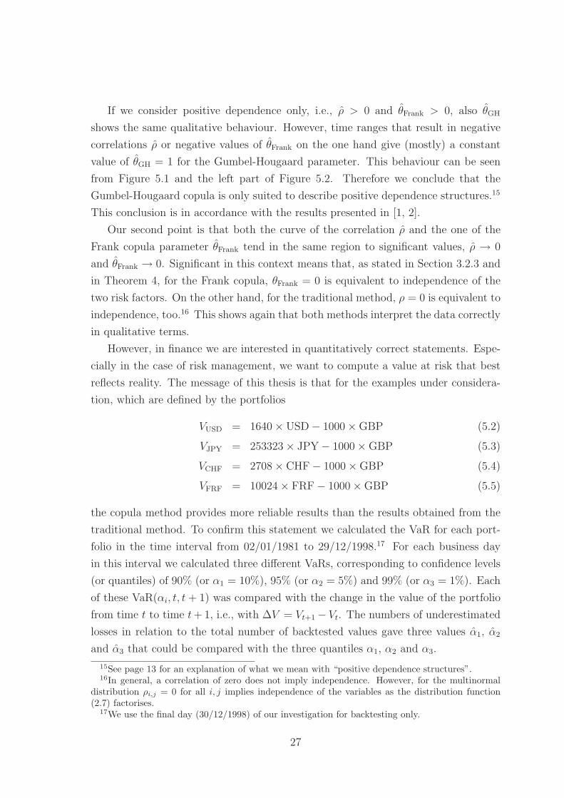
If we consider positive dependence only, i.e., ρ > 0 and θFrank > 0, also θGH

shows the same qualitative behaviour. However, time ranges that result in negative

correlations ρ or negative values of θFrank on the one hand give (mostly) a constant

value of θGH = 1 for the Gumbel-Hougaard parameter. This behaviour can be seen

from Figure 5.1 and the left part of Figure 5.2. Therefore we conclude that the

Gumbel-Hougaard copula is only suited to describe positive dependence structures.15

This conclusion is in accordance with the results presented in [1, 2].

Our second point is that both the curve of the correlation ρ and the one of the

Frank copula parameter θFrank tend in the same region to significant values, ρ → 0

and θFrank → 0. Significant in this context means that, as stated in Section 3.2.3 and

in Theorem 4, for the Frank copula, θFrank = 0 is equivalent to independence of the

two risk factors. On the other hand, for the traditional method, ρ = 0 is equivalent to

independence, too.16 This shows again that both methods interpret the data correctly

in qualitative terms.

However, in finance we are interested in quantitatively correct statements. Espe-

cially in the case of risk management, we want to compute a value at risk that best

reflects reality. The message of this thesis is that for the examples under considera-

tion, which are defined by the portfolios

VUSD = 1640 × USD − 1000 × GBP (5.2)

VJPY = 253323 × JPY − 1000 × GBP (5.3)

VCHF = 2708 × CHF − 1000 × GBP (5.4)

VFRF = 10024 × FRF − 1000 × GBP (5.5)

the copula method provides more reliable results than the results obtained from the

traditional method. To confirm this statement we calculated the VaR for each port-

folio in the time interval from 02/01/1981 to 29/12/1998.17 For each business day

in this interval we calculated three different VaRs, corresponding to confidence levels

(or quantiles) of 90% (or α1 = 10%), 95% (or α2 = 5%) and 99% (or α3 = 1%). Each

of these VaR(αi, t, t + 1) was compared with the change in the value of the portfolio

from time t to time t + 1, i.e., with ∆V = Vt+1 − Vt. The numbers of underestimated

losses in relation to the total number of backtested values gave three values α1, α2

and α3 that could be compared with the three quantiles α1, α2 and α3.

15See page 13 for an explanation of what we mean with “positive dependence structures”.16In general, a correlation of zero does not imply independence. However, for the multinormal

distribution ρi,j = 0 for all i, j implies independence of the variables as the distribution function(2.7) factorises.

17We use the final day (30/12/1998) of our investigation for backtesting only.

27

1 3 5 7 9 11 13 15 0%

1%

2%

3%

4%

5%

6%

7%

8%

9%

10%

11%

# MC steps / 100

back

test

ing

failu

reTraditional Monte Carlo VaR

1 3 5 7 9 11 13 15 0%

1%

2%

3%

4%

5%

6%

7%

8%

9%

10%

11%

# MC steps / 100ba

ckte

stin

g fa

ilure

Monte Carlo VaR using Frank

copula and t−distr. margins

Figure 5.3: Backtesting results of the USD portfolio (5.2), using the traditionalmethod (left) and the copula method (right) for quantiles α1 = 10% (green squares),α2 = 5% (red circles) and α3 = 1% (blue triangles) and various numbers of MC steps.

To test the dependence of the numerical results on the number of Monte Carlo

steps, we did this investigation for various numbers of MC steps ranging from 100

to 1500. For the USD portfolio (5.2), we present our results of the underestimated

losses in Table 5.2. The data that are listed in this table were obtained from a tradi-

tional Monte Carlo simulation on the one hand (i.e., Gaussian copula and normally

distributed margins) and from MC simulations using both the Frank and the Gumbel-

Hougaard copula on the other hand. The margins used with the copula methods were

t-distributions. In Figure 5.3 we show the data of the traditional method and of the

copula method, using the Frank copula.

First, we want to emphasise that, once a number of MC steps of about 500 is

reached, the data do not change significantly under any additional increase of the

number of MC steps. This behaviour can be observed for both algorithms, each

copula and each confidence level, as one can see from Table 5.2. Therefore numerical

results for numbers of MC steps of O(1000) seem to be reliable and are suited as a

basis for a discussion and comparison of the two methods.

Secondly, and this is the most important point that we want to emphasise, the

backtesting results show that the copula method works better then the traditional

method for each confidence level. As mentioned in Chapter 1, “better” in this context

28

percentage of underestimated losses

traditional Monte CarloMC with Gumbel-Hougaardcopula and t-distr. margins

MC with Frank copulaand t-distr. margins

no. ofMC-steps

α1 = 10% α2 = 5% α3 = 1% α1 = 10% α2 = 5% α3 = 1% α1 = 10% α2 = 5% α3 = 1%

100 9.35% 5.34% 2.28% 10.46% 5.76% 1.86% 10.77% 5.99% 1.80%

200 8.82% 4.68% 1.84% 9.98% 5.03% 1.35% 10.31% 5.36% 1.44%

300 8.60% 4.61% 1.71% 9.82% 4.99% 1.22% 10.06% 5.14% 1.15%

400 8.62% 4.63% 1.64% 9.73% 4.90% 1.15% 9.91% 5.05% 1.00%

500 8.60% 4.63% 1.68% 9.73% 4.79% 1.11% 9.93% 4.94% 1.00%

600 8.67% 4.72% 1.62% 9.71% 4.74% 1.06% 9.82% 4.88% 0.95%

700 8.67% 4.68% 1.62% 9.71% 4.81% 1.09% 9.82% 4.94% 1.00%

800 8.69% 4.68% 1.62% 9.64% 4.74% 1.02% 9.84% 4.92% 1.00%

900 8.73% 4.66% 1.55% 9.67% 4.83% 1.06% 9.80% 4.99% 1.00%

1000 8.73% 4.70% 1.62% 9.62% 4.72% 1.06% 9.86% 4.92% 1.02%

1100 8.65% 4.63% 1.66% 9.69% 4.72% 1.06% 9.86% 4.90% 0.93%

1200 8.58% 4.61% 1.64% 9.75% 4.77% 1.02% 9.93% 5.01% 0.98%

1300 8.62% 4.61% 1.62% 9.67% 4.81% 0.98% 9.86% 4.99% 0.91%

1400 8.76% 4.61% 1.62% 9.64% 4.70% 0.95% 9.86% 4.85% 0.89%

1500 8.71% 4.61% 1.62% 9.62% 4.74% 0.98% 9.93% 4.92% 0.89%

Tab

le5.2:

Back

testing

results

ofth

eU

SD

/GB

Pportfolio,

usin

gth

etrad

itional

meth

od

and

the

copula

meth

od

forth

eFran

kan

dth

eG

um

bel-H

ougaard

copula,

forquan

tilesα

1=

10%,α

2=

5%an

dα

3=

1%,an

dvariou

snum

bers

ofM

Cstep

s.

29

means that the deviation of the percentage of the backtesting failures αi from the

quantiles αi is smaller in the case of the copula method than in the case of the

traditional method for each i = 1, 2, 3.

To quantify the last statement, we consider below the results that we obtained

from simulations using 1500 Monte Carlo steps. Again, the quantiles under inves-

tigation were α1 = 10%, α2 = 5% and α3 = 1%. In Table 5.3 we summarise the

corresponding percentages of underestimated losses αi for the four portfolios (5.2)-

(5.5) for i = 1, 2, 3. For the copula method, we used both the Frank copula and

the Gumbel-Hougaard copula. In addition, each copula was used with margins that

obey a normal distribution on the one hand (see below) and a t-distribution on the

other hand. Beside the results that we have obtained from the traditional and the

copula Monte Carlo methods, we also present in Table 5.3 backtesting results that

were based on the variance-covariance method and on historical simulation.18

We do the comparison of the backtesting results using the quantity

χ2 ≡3

∑

i=1

(

αi − αi

αi

)2

. (5.6)

Its values for the various VaR methods just mentioned and for each portfolio are also

listed in Table 5.3.

The first statement we want to make is that the copula method results in more

reliable results than the traditional method for each portfolio under consideration if

the copula method is used with t-distributed margins. Whereas the deviation χ2 lies

in the range χ2 ∼ 0.2−0.4 for the traditional method, it lies between 0.005 and 0.034

for the copula method with t-distributed margins.

Next we turn our attention to the copula method in combination with Gaussian

margins. In anticipation of our results, stating that the copula method (i.e., using a

copula and t-distributed margins) works better, we have not mentioned this method so

far. It simply describes the use of a copula in combination with normally distributed

margins. In the language of Chapters 2 and 4, the copula method in combination with

Gaussian margins consists of steps 1-4 and 8 of the traditional method and steps 5-7

of the copula method. In this case, the deviation χ2 is approximately χ2 ∼ 0.1−0.45.

This is the same order of magnitude as the results obtained from the traditional

method. A one by one comparison of the eight values under consideration (four

portfolios times two copulas) shows that the copula method with Gaussian margins

gives more reliable results in five cases.

18Both the variance-covariance method and historical simulation are not explained in this thesis.An overview of both methods can be found in [4], a detailed discussion in [9], for example.

30

percentage of underestimated losses

portfolio quantileshistoricalsimulation

variance-covariance

tradition-al MC

MC GH,Gaussianmargins

MC GH,t-distr.margins

MC Frank,Gaussianmargins

MC Frank,t-distr.margins

10% 10.33% 8.60% 8.71% 8.60% 9.62% 9.75% 9.93%

1640 USD 5% 5.32% 4.63% 4.61% 4.34% 4.74% 5.03% 4.92%

-1000 GBP 1% 1.22% 1.40% 1.62% 1.29% 0.98% 1.40% 0.89%

χ2 0.0533 0.1822 0.4049 0.1184 0.0047 0.1579 0.0131

10% 10.77% 8.22% 8.71% 8.71% 10.02% 9.33% 10.02%

253323 JPY 5% 5.52% 4.34% 4.61% 4.43% 5.28% 5.10% 5.39%

-1000 GBP 1% 1.33% 1.22% 1.44% 1.26% 1.17% 1.35% 1.13%

χ2 0.1257 0.0968 0.2171 0.0989 0.0336 0.1289 0.0230

10% 10.04% 7.76% 7.74% 8.25% 10.33% 7.71% 9.64%

2708 CHF 5% 5.03% 3.99% 4.08% 4.10% 4.83% 4.12% 4.50%

-1000 GBP 1% 1.04% 1.37% 1.35% 1.57% 1.17% 1.35% 1.02%

χ2 0.0018 0.2312 0.2092 0.3925 0.0328 0.2071 0.0117

10% 9.98% 7.07% 6.94% 7.32% 9.29% 7.92% 9.40%

10024 FRF 5% 4.99% 4.13% 4.15% 4.24% 5.08% 4.41% 4.95%

-1000 GBP 1% 1.11% 1.35% 1.44% 1.60% 1.11% 1.55% 0.93%

χ2 0.0119 0.2407 0.3176 0.4514 0.0171 0.3623 0.0084

Tab

le5.3:

Com

parison

ofth

evariou

sV

aRm

ethods.

31

With these results at hand we come to the following conclusions:

• The bare change of the joint distribution function, leaving the distribution func-

tions of the margins unchanged, i.e., the change from the traditional method to

the copula method with Gaussian margins may improve the VaR calculation a

little if one is using the Frank copula or the Gumbel-Hougaard copula.

• The change of the distribution functions of the margins from Gaussian margins

to t-distributed margins makes the VaR calculations much more reliable: αi lies

much closer to αi for the copula method with t-distributed margins than for the

traditional method for each i = 1, 2, 3. Therefore χ2 is between one and two

orders of magnitude smaller for the copula method with t-distributed margins

than for the traditional method. These statements hold for both the Frank and

the Gumbel-Hougaard copula.

• The use of copulas is necessary if one wants to consider arbitrary distribution

functions of the margins.

• The backtesting failures that we obtain for the USD portfolio (5.2) for the whole

time period under consideration result in a smaller value of χ2 in the case of the

Gumbel-Hougaard copula than in the case of the Frank copula. For the other

three portfolios (5.3) - (5.5), the results of the Frank copula are more reliable.

The reason for this behaviour is the (strong) positive dependence between the

USD/DEM rate and the GBP/DEM rate during that time period. For most

dates within that period the correlation between these two risk factors, mea-

sured over 250 business days, is greater than zero.19 In contrast, the correlations

between the JPY/DEM rate, the CHF/DEM rate and the FRF/DEM rate on

the one side and the GBP/DEM rate on the other side, measured over 250 busi-

ness days, are less than zero for a significant number of dates within the whole

time period under consideration.20 For the correlation between the CHF/DEM

rate and the GBP/DEM rate, for example, this behaviour is presented by the

green line in Figure 5.1.

19The strong positive dependence between the USD/DEM rate and the GBP/DEM rate can alsobe seen if one takes a look on the correlations between these risk factors, based on all data in theperiod 02/01/1980 to 30/12/1998. It is given by ρUSD,GBP = 0.415.

20The correlations between the JPY/DEM rate, the CHF/DEM rate and the FRF/DEM rate onthe one side and the GBP/DEM rate on the other side, based on all data in the period 02/01/1980to 30/12/1998, are given by ρJPY,GBP = 0.179, ρCHF,GBP = 0.040 and ρFRF,GBP = 0.164.

32

−0.03 −0.015 0 0.015 0.030

20

40

60

80

100

120

r

f(r)

−0.03 −0.025 −0.02 −0.0150

1

2

3

r

f(r)

Figure 5.4: Histogram of relative GBP/DEM rates and approximations of the datausing a t-distribution (red line) with k = 4 and a Gaussian distribution (blue line).The right picture shows a magnified detail of the left picture.

As the estimator θGH of the Gumbel-Hougaard copula parameter becomes one

for a data sample that shows a negative dependence structure and because

θGH = 1 equals the product copula (see (3.13)), all data with any negative

dependence structure will be treated by the Gumbel-Hougaard copula as if they

were independent due to Theorem 4 (page 18). Therefore the pseudo random

numbers, that have to be generated within a Monte Carlo calculation of the

value at risk, do not show the correct dependence structure.

The comparison of the two copula methods, using the Gumbel-Hougaard copula

on the one hand and the Frank copula on the other hand, shows that the Frank

copula should be preferred in general. In situations where the data under inves-

tigation show a (strong) positive dependence structure, the Gumbel-Hougaard

copula may also be used. Again, this in accordance with [1, 2].

As the main improvement of the VaR calculation comes from the replacement

of the Gaussian margins by t-distributed margins, we want to investigate this point

in some more detail. In Figure 5.4 we show a normalised histogram of the relative

GBP/DEM rates, based on 4759 data points that can be obtained from the period

02/01/1980 to 30/12/1998. In addition, we show in the same figure the density

functions of the corresponding t-distribution and of the corresponding Gaussian dis-

tribution. The estimated parameters for both distributions are µGBP = −0.0000528

33

1982 1984 1986 1988 1990 1992 1994 1996 19981

10

100

date

k (250 days)

↑k (19 years)

Figure 5.5: Estimator of the index k of the t-distribution of the relative GBP/DEMrates, measured over 250 business days (blue points) and measured over the period02/01/1980 to 30/12/1998 (red line).

and σGBP = 0.00500. For the t-distribution we have kGBP = 4. As one can see

from Figure 5.4, the t-distribution describes the data much better than the Gaussian

distribution. This is both true for the region around the mean of the distribution,

which is obvious from the left part of Figure 5.4, and for the tail behaviour, as can

be seen from the right part of Figure 5.4. As the tail behaviour is relevant for VaR

calculations, we will come back to it during the discussion of Figure 5.6.

As step number four of the copula method (see page 21) states that the estimator of

the parameter k of the t-distribution of each margin has to be calculated for each time

step, we present in Figure 5.5 the evolution of k of the relative GBP/DEM rates. The

blue points that are shown in Figure 5.5 are based on 250 business days, in agreement

with our VaR calculations. One can see from this semilogarithmic plot that k lies

between three and ten for most of the dates. As a Gaussian distribution corresponds

to k → ∞, we conclude that the relative GBP/DEM rates can be described much

better by a t-distribution with a small number k than by a Gaussian distribution

in the period 02/01/1980 to 31/12/1998. We observed the same behaviour for the

relative FX rates USD/DEM, JPY/DEM CHF/DEM and FRF/DEM.

We already mentioned that two additional methods exist to compute the VaR, the

variance-covariance method and historical simulation. We now compare our numerical

34

results with the analytical results (see Table 5.3 again) obtained using these methods.

We first take a look on the backtesting results of the variance-covariance method.

As expected, the values of αi lie very close to the corresponding values that we

obtained from the traditional method for each i = 1, 2, 3. This can be seen as a

kind of consistence check of the algorithm of the traditional method as, in the case

of a portfolio which is a linear combination of the risk factors (see equation (5.1)),

the variance-covariance VaR is the limit of the traditional Monte Carlo VaR for an

infinite number of MC steps. Because of this fact, the VaR results obtained from

the variance-covariance method are also less reliable than the VaR results from the

copula method.

Let us now discuss the historical simulation results. As one can see from Ta-

ble 5.3, the backtesting results are much better than in the case of the traditional

method, slightly better than the results obtained from the copula method with Gaus-

sian margins and about as good as the results obtained from the copula method using

t-distributed margins. The high quality of the backtesting results obtained from the

historical simulation is well known [9]. Its reason is given by the simplicity of the

historical simulation. This method does not need any model to describe the risk

factors and the dependence between different risk factors, i.e., one can neglect any

systematic errors due to model assumptions. In addition, no approximations (e.g.,

linear approximation) have to be used within the VaR calculation.

To get a deeper understanding of our numerical results, we now come back to the

traditional method and the copula method with t-distributed margins. In the upper

left part of Figure 5.6 we present the relative FX rates USD/DEM vs. GBP/DEM,

measured during the whole period under investigation, i.e., in the period 02/01/1980

to 30/12/1998. Based on these data points we estimated the parameters of the

distributions. For the relative FX rates GBP/DEM they are given on page 33. For

the relative FX rates USD/DEM we obtained µUSD = 0.0000216 and σUSD = 0.00732

for both distributions and kUSD = 6 for the t-distribution.

With the parameters of the margins at hand we generated three sets of pairs of

pseudo random numbers. Each of these sets contains 4759 pairs of PRNs, i.e., the

same number of data as provided by the historical data.

The first set of PRNs was generated according to the traditional method, i.e., the

pairs of PRNs were generated according to a binormal distribution. The correlation

that we used to generate the PRNs is ρUSD,GBP = 0.415, as already given on page 32.

We present these PRNs in the lower left part of Figure 5.6. A comparison of this

figure with the historical data points provides a good hint for the rather bad quality

35

−0.06 −0.03 0 0.03 0.06−0.06

−0.03

0

0.03

0.06

rUSD

rGBP

relative FX−rates USD/DEM vs. GBP/DEM

(02.01.1980 − 30.12.1998 = 4759 data points)

−0.06 −0.03 0 0.03 0.06−0.06

−0.03

0

0.03

0.06

r1

r2

4759 PRNs, acc. to Gumbel−Hougaard

copula with t−distributed margins

−0.06 −0.03 0 0.03 0.06−0.06

−0.03

0

0.03

0.06

r1

r2

4759 PRNs, acc. to Gaussian

copula with Gaussian margins

−0.06 −0.03 0 0.03 0.06−0.06

−0.03

0

0.03

0.06

r1

r2

4759 PRNs, acc. to Frank

copula with t−distributed margins

Figure 5.6: Historical data of relative FX rates USD/DEM vs. GBP/DEM and cor-responding pseudo random numbers, according to the traditional method and thecopula method. See text for more details.

of the backtesting results, obtained with the traditional method. Even if the shape

of the PRNs21 around the mean is similar to the one of the historical data, extreme

data points are missing in the lower left part of Figure 5.6. This is a consequence of

the low tails of Gaussian distributions. However, the tail dependence is crucial for a

VaR calculation. Especially in our case of a linear portfolio (5.1), the values of the

simulated pairs of PRNs are directly related to the profits and losses of the portfolio.

Let us now turn to the right part of Figure 5.6. There we present pairs of PRNs

that were generated according to t-distributions (with parameters as given above)

that were linked together by copulas. For the upper right part of Figure 5.6 we used

the Gumbel-Hougaard copula with θGH;USD,GBP = 1.401, for the lower right part we

used the Frank copula with θFrank;USD,GBP = 3.077. One can see immediately that

both copula pictures contain many more outliers than the traditional picture. The

reason for this are the fat tails of the t-distributions. Although the outliers in the

copula pictures are not in the same places as in the historical picture, they give

a better approximation of the historical picture than the traditional picture. As a

consequence, the copula method in conjunction with t-distributed margins provides

21The PRNs that have been generated using the binormal distribution yield a figure that resemblesan ellipsoid. This behaviour is well known in statistics and can therefore be used as additionalevidence that our numerical Monte Carlo algorithm works fine in the traditional case.

36

VaR results that are much more reliable than the VaR results obtained from the

traditional method.

We finally want to make a remark on the three sets of PRNs that are shown

in Figure 5.6. As described in step 7 of the copula method (see page 23) and in

Appendix A.3 (see equations (A.15) and (A.16)), the starting point for all these PRNs

are independent, in [0, 1] uniformly distributed PRNs. To ensure a fair comparison,

we used the same set of these PRNs to generate the lower left part, the upper right

part and the lower right part of Figure 5.6.

37

Chapter 6

Summary and Conclusions

In this thesis we have demonstrated an alternative method to compute the value at

risk of a financial portfolio. For this purpose, we have introduced the concept of

copulas and presented the most important properties of these functions. For the sake

of simplicity, we have restricted ourselves to two risk factors and therefore to two-

dimensional copulas only. We have discussed two representatives of the copula family

in detail, the Frank copula and the Gumbel-Hougaard copula. Using this tool, we

have modified two basic assumptions underlying the common method of computing

the VaR using Monte Carlo techniques: usually, the dependence structure between

two risk factors is assumed to be described by the correlation between these factors.

Particularly, the joint distribution is assumed to be of the binormal kind. We have

replaced this dependence structure by a dependence structure that is defined by one

of the two copulas mentioned above. In doing so, we have replaced the role of the

correlation ρ by the parameters θFrank and θGH that determine the behaviour of the

copulas. Secondly, we have replaced the assumption that each risk factor obeys a

normal distribution by the assumption of t-distributed margins.

To test whether the copula ansatz improves the computation of the VaR, we

have considered four simple linear portfolios which consist of the FX rate GBP/DEM

and one out of the FX rates USD/DEM, JPY/DEM, CHF/DEM and FRF/DEM.

Assuming confidence levels of 90%, 95% and 99%, we have calculated the VaRs for

these portfolio on the basis of 250 banking days, using the following methods:

• traditional Monte Carlo simulation;

• copula Monte Carlo simulation, using both normally distributed margins and t-

distributed margins and using both the Frank copula and the Gumbel-Hougaard

copula;

38

• the variance-covariance method;

• historical simulation.

The computations and the corresponding backtesting of the results have been per-

formed on the basis of historical FX rates ranging over nineteen years. This means

that our backtesting statistics are based on approximately 4750 measurements.

The results that we have obtained in this thesis show that, at least for the portfolios

under consideration, the copula method in conjunction with t-distributed margins

is more reliable than both the traditional Monte Carlo method and the variance-

covariance method. In other words, for each confidence level the absolute deviations

of the percentages of the backtesting failures from the quantiles are smaller in the

case of the copula method than both in the case of the traditional method and in the

case of the variance-covariance method.

A comparison of the copula method with t-distributed margins with the historical

simulation shows that both methods result in VaR values that are of the same quality.

The backtesting values of these methods lie very close to the predicted values and

very close to each other.

With these results at hand we now want to formulate the answers to the three

questions that were asked in the introduction. The first question asked for the ap-

propriate marginal distributions of the risk factors. Based on our numerical data the

answer has to be that, for the most dates within the nineteen years of investigation,

the five FX rates under consideration can be described very well by t-distributions

with a parameter k that is less than or equal ten. Particularly, the margins do not

show a Gaussian behaviour, which corresponds to k → ∞.

The second question asked for the appropriate joint distribution of the risk factors.

As discussed in detail in the previous chapter, a binormal distribution describes the

data well in the sense that the shape of the distribution resembles the shape of

the historical data. However, extreme values are missing if one uses a binormal

distribution. Therefore we suggest the Frank copula to describe the joint distribution.

In addition, if one is dealing with margins that show a positive dependence structure,

the joint distribution can also be described by the Gumbel-Hougaard copula.

The content of the third question was of a more technical nature. It concerned a

possibility of simulating pseudo random numbers using these marginal distributions

and this joint distribution. Whereas the necessary tools to generate independent

PRNs according to a t-distribution are given in Appendix A.1 and Appendix B,

Chapter 4 describes in detail how to generate pairs of PRNs (with arbitrary margins)

39

using a copula dependence structure. Furthermore, we have given detailed infor-

mation on what an algorithm looks like in the case of the Frank copula and the

Gumbel-Hougaard copula.

We finally want to summarise the application of copulas and the t-distribution in

financial risk management. In this thesis it has been shown that the use of copulas

and the t-distribution may improve the reliability of the VaR calculation of a financial

portfolio. To be able to decide whether or not one should prefer the copula method

to the traditional method, a supplementary investigation of the speed of the proposed

copula algorithm would be useful. As we considered two risk factors only, a natural

extension of studies in this field would have to include three or more risk factors.

Furthermore, there is a large number of other copulas [3], some of which also may

be suited for use in a VaR computation. Finally one could test additional marginal

distributions. For example, this might be necessary if one is using risk factors that

are different from FX rates. As discussed in detail, due to the use of copulas one is

completely free in the choice of the marginal distribution. The last point might be

the biggest advantage when applying copulas to the computation of the value at risk.

40

Appendix A

Generation of Pseudo RandomNumbers

In this appendix we deal with the generation of pseudo random numbers. At first

we present a method that is based on the transformation of variables. It can be

used for the generation of PRNs that obey an univariate distribution for which one

can compute the inverse distribution function either analytically or numerically. In

the next section we summarise the Box-Muller method. It shows how to generate

normally distributed PRNs. We end this chapter with a generalisation of the Box-

Muller method for the simultaneous generation of tuples of PRNs that are distributed

according to a multivariate normal distribution.

All methods that we discuss are based on the assumption that one is able to

generate independent PRNs that are uniformly distributed in the [0, 1] interval. As

it is not within the scope of this thesis, we do not describe how to generate these

numbers. The interested reader may find several algorithms describing this topic in

any good text book on numerical statistics (see, for example, [11]).

A.1 Transformation of Variables

A general method to generate PRNs according to a given distribution uses a trans-

formation of variables to obtain these numbers from uniformly distributed PRNs.

Starting with a uniformly distributed PRN u ∈ [0, 1] we want to generate a PRN

r = r(u) with a given distribution f(r),

∫ b

a

dr f(r) = 1 . (A.1)

41

First we equalise the integrated probability density to u,

F (r) =

∫ r

a

dr′ f(r′) = u . (A.2)

We next have to invert the distribution function F . Then

r(u) = F−1(u) (A.3)

is the PRN with the desired distribution. In cases where the computation of F−1

cannot be done analytically one either has to compute (A.3) numerically or one has

to use a different algorithm for the generation of the PRNs, e.g., the Box-Muller

method for normally distributed PRNs.

A.2 The Box-Muller Method

We now shortly summarise what is known in literature as the Box-Muller method.

This refers to an algorithm which is used to generate simultaneously two independent

normally distributed PRNs from two independent uniformly distributed PRNs.

Assume that we want to generate r1 from a N (µ1, σ21) distribution and r2 from a

N (µ2, σ22) distribution.22 If we denote the two uniformly distributed PRNs by u1 and

u2, the introduction of polar coordinates, followed by a variable transformation as in

A.1, shows (see [11] for details) that r1 and r2 are given by

r1 =√

−2σ21 ln u1 sin(2π u2) + µ1 , (A.4)

r2 =√

−2σ22 ln u1 cos(2π u2) + µ2 . (A.5)

A.3 Pseudo Random Numbers According to the

Multinormal Distribution

Below we will discuss how to generate a multivariate normal distribution of n corre-

lated PRNs represented by a vector ~r. The density function we have to consider is

presented in equation (2.7).

The basic idea behind generating the desired PRNs is to apply what is called

Cholesky decomposition [14] to the inverse covariance matrix, provided that the inverse

exists. The ansatz of this decomposition is

C−1 = AtA , (A.6)

22See equation (2.2) on page 6 for the density function N (µi, σ2i ) of a normal distribution.

42

where C is given by (2.9). The matrix A in (A.6) is a lower triangular matrix,

A =

α1,1 0 · · · 0

α2,1 α2,2. . .

......

.... . . 0

αn,1 αn,2 · · · αn,n

. (A.7)

Using (A.6) we now perform a linear variable transformation in (2.7),

~r → ~s = A (~r − ~µ) . (A.8)

One can show that the corresponding determinant of the Jacobian matrix is given by

∂(r1, . . . , rn)

∂(s1, . . . , sn)=

√det C . (A.9)

Therefore, the transformed density function takes the form

f(~s) =1

√

(2π)nexp

{

−1

2~s t ~s

}

=n

∏

i=1

1√2π

exp

{

−1

2s2

i

}

. (A.10)

Equation (A.10) is the density function of n uncorrelated, standard normally dis-

tributed variables. Therefore the simultaneous generation of n correlated, normally

distributed PRNs is achieved in two steps:

(a) Generate n uncorrelated, standard normally distributed PRNs s1, . . . , sn using

the Box-Muller method presented in Section A.2.

(b) Compute the desired PRNs r1, . . . , rn by the reverse transformation of (A.8),

~s → ~r = A−1~s + ~µ . (A.11)

As we only need the two-dimensional case in this thesis, we will now focus on

the generation of bivariate normally distributed PRNs. The n-dimensional case is a

simple generalisation and can be found, for example, in [9].

The first step is (see equations (A.4) and (A.5)):

(a) Generate two uncorrelated, standard normally distributed PRNs

s1 =√

−2 ln u1 sin(2π u2) and (A.12)

s2 =√

−2 ln u1 cos(2π u2) (A.13)

from two uncorrelated PRNs u1 and u2 that are uniformly distributed in [0, 1].

43

From (2.9), (A.7) and condition (A.6) one can show that A can be written as

A =1√

det C

(

σ2

√

1 − ρ2 0−ρ σ2 σ1

)

(A.14)

where det C = σ21σ

22 (1 − ρ2) and ρ denotes the correlation coefficient (see (2.11)),

ρ = ρ1,2 = c1,2/(σ1σ2). The correlation is normalised so it can take all values in the

interval [−1, 1]. For ρ = ±1 expression (A.14) is not defined. However, in this section

we can neglect these cases as ρ = ±1 means that the variables r1 and r2 are completely

positively or negatively correlated. In this case we only have to simulate one PRN

using the method described in Section A.2. The second PRN will be deterministic.

From (A.11) and (A.14) one finds that the second step mentioned above becomes:

(b) Perform the variable transformation s1, s2 → r1, r2 as follows:

r1 = σ1 s1 + µ1 and (A.15)

r2 = σ2 (ρ s1 +√

1 − ρ2 s2) + µ2 . (A.16)

r1 and r2 are the two desired, correlated PRNs that obey a bivariate normal

distribution.

44

Appendix B

The t-Distribution

In this appendix we summarise some features of the so-called Student-distribution or

t-distribution [15].

B.1 The Density Function

Let us start directly with the density function of a t-distribution with k degrees of

freedom,

hk(r) =Γ

(

k+12

)

Γ(

k2

)

Γ(

12

)√k

(

1 +r2

k

)

−k+12

. (B.1)

To keep things simple, we restrict ourselves to k = 1, 2, 3, . . .. Therefore we only need

the following features of the Γ-function:

Γ(1) = 1

Γ

(

1

2

)

=√

π (B.2)

Γ(k + 1) = k Γ(k)

It is well known in statistics [15] that the t-distribution converges as k → ∞ to

the standard normal distribution N (0, 1),

limk→∞

hk(r) =1√2π

exp

{

−r2

2

}

. (B.3)

Motivated by this property we perform the following variable transformation,

r → r − µ

γ. (B.4)

Under this transformation, the t-distribution becomes

fk(r) =1

γhk

(

r − µ

γ

)

=Γ

(

k+12

)

Γ(

k2

)

Γ(

12

)√k γ

(

1 +(r − µ)2

k γ2

)

−k+12

, (B.5)

45

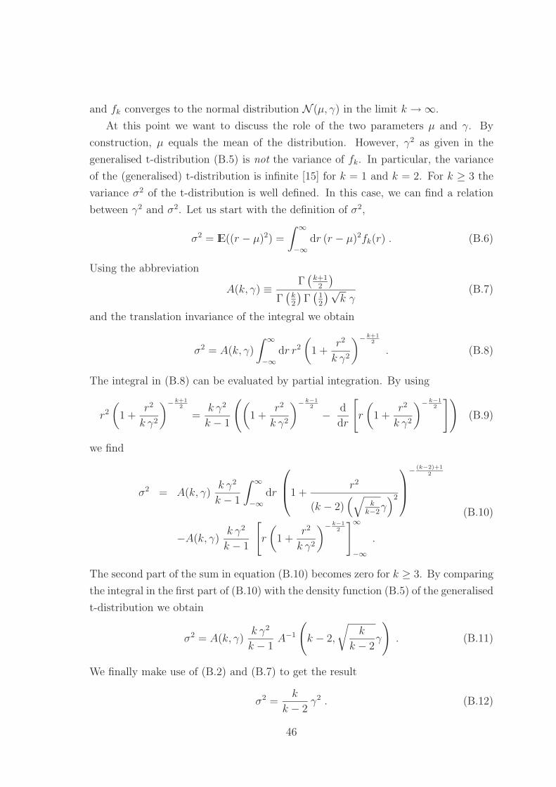
and fk converges to the normal distribution N (µ, γ) in the limit k → ∞.

At this point we want to discuss the role of the two parameters µ and γ. By

construction, µ equals the mean of the distribution. However, γ2 as given in the

generalised t-distribution (B.5) is not the variance of fk. In particular, the variance

of the (generalised) t-distribution is infinite [15] for k = 1 and k = 2. For k ≥ 3 the

variance σ2 of the t-distribution is well defined. In this case, we can find a relation

between γ2 and σ2. Let us start with the definition of σ2,

σ2 = IE((r − µ)2) =

∫

∞

−∞

dr (r − µ)2fk(r) . (B.6)

Using the abbreviation

A(k, γ) ≡ Γ(

k+12

)

Γ(

k2

)

Γ(

12

)√k γ

(B.7)

and the translation invariance of the integral we obtain

σ2 = A(k, γ)

∫

∞

−∞

dr r2

(

1 +r2

k γ2

)

−k+12

. (B.8)

The integral in (B.8) can be evaluated by partial integration. By using

r2

(

1 +r2

k γ2

)

−k+12

=k γ2

k − 1

(

(

1 +r2

k γ2

)

−k−12

− d

dr

[

r

(

1 +r2

k γ2

)

−k−12

])

(B.9)

we find

σ2 = A(k, γ)k γ2

k − 1

∫

∞

−∞

dr

1 +

r2

(k − 2)(√

kk−2

γ)2

−(k−2)+1

2

−A(k, γ)k γ2

k − 1

[

r

(

1 +r2

k γ2

)

−k−12

]∞

−∞

.

(B.10)

The second part of the sum in equation (B.10) becomes zero for k ≥ 3. By comparing

the integral in the first part of (B.10) with the density function (B.5) of the generalised

t-distribution we obtain

σ2 = A(k, γ)k γ2

k − 1A−1

(

k − 2,

√

k

k − 2γ

)

. (B.11)

We finally make use of (B.2) and (B.7) to get the result

σ2 =k

k − 2γ2 . (B.12)

46

In other words, γ is a parameter which influences the shape of the generalised t-

distribution and which is related to the variance σ2 via equation (B.12).

From (B.12) we again obtain the expected behaviour of γ2 in the limit k → ∞,

i.e., γ2 → σ2, which is due to the fact that the t-distribution converges to the normal

distribution.

Inserting (B.12) into (B.5) results in the following equation for the density function

of the generalised t-distribution:

fk(r) =Γ

(

k+12

)

Γ(

k2

)

Γ(

12

)√k − 2 σ

(

1 +(r − µ)2

(k − 2) σ2

)

−k+12

for k ≥ 3 (B.13)

B.2 The Distribution Function

In this section we describe the computation of the cumulative density function of the

generalised t-distribution. As the equations that we present in the following are valid

for all k ≥ 1, we use equation (B.5) instead of (B.13) to describe the density function.

With the abbreviation (B.7) the quantity we are interested in is given by

Fk(r) =

∫ r

−∞

dr′ fk(r′) = A(k, γ)

∫ r

−∞

dr′(

1 +(r′ − µ)2

k γ2

)

−k+12

. (B.14)

Let us define

I(r; a, b, k) ≡∫ r

−∞

dr′(

r′2+ ar′ + b

)

−k+12

. (B.15)

Then we have

Fk(r) = A(k, γ)(

k γ2)

k+12 I(r;−2µ, k γ2 + µ2, k) . (B.16)

The remaining task is to compute the function I. This can be done recursively. The

two initial conditions are given by [15]

I(r; a, b, 1) =2√

4b − a2

[

arctan

(

2r + a√4b − a2

)

+π

2

]

and

I(r; a, b, 2) =2

4b − a2

(

2r + a√r2 + ar + b

+ 2

)

.(B.17)

Furthermore, the recursive formula for k ≥ 3 is [15]

I(r; a, b, k) =4r + 2a

(k − 1)(4b − a2)(r2 + ar + b)−

k−12 +

4k − 8

(k − 1)(4b − a2)I(r; a, b, k − 2) .

(B.18)

47

Appendix C

The Maximum Likelihood Method

In statistical data analysis, a common problem is to determine a probability density

function f of which only the functional form is known, while its parameters are

unknown. Let us assume that f depends on n variables r1, . . . , rn and contains k

parameters p1, . . . , pk. We write f in the form f(r1, . . . , rn ; p1, . . . , pk). Let us further

assume that a set of N (historical) data, ~rj ≡ (r1,j, . . . , rn,j)t where j = 1, . . . , N , is

available that obeys the probability density function. The task is therefore to estimate

the parameters p1, . . . , pk on the basis of these N data tuples.

For some probability density functions, the estimators of the parameters are well

known. For example, the parameters of the multinormal distribution function (2.7)

are the means and the variances of the variables and the correlations between the

variables. On the basis of a set of historical data, unbiased and consistent estimators

for these parameters are given by expressions (2.4), (2.5) and (2.12). However, it

is not always possible to find an analytical form to calculate parameter estimators

directly from historical data. For these probability density functions, the maximum

likelihood method [11] (ML method) provides a solution.

C.1 Theoretical Background

The quantity of central importance in the maximum likelihood method is given by

the likelihood function

L(~r1, . . . , ~rN ; p1, . . . , pk) ≡N∏

j=1

f(~rj ; p1, . . . , pk) . (C.1)

The maximum likelihood method states that the particular k-tuple (p1, . . . , pk) at

which L reaches its maximum is a good estimator of the “real” k-tuple (p1, . . . , pk). In

other words, we have to find a k-tuple (p1, . . . , pk) so that L(~r1, . . . , ~rN ; p1, . . . , pk) <

48

L(~r1, . . . , ~rN ; p1, . . . , pk) for all possible (p1, . . . , pk) where (p1, . . . , pk) 6= (p1, . . . , pk).

Here we assume that the likelihood function contains one unique maximum only. As

this is, of course, not true in general, we will come back to this point later in this

section.

From the above discussion it is obvious that (p1, . . . , pk) is a function of ~r1, . . . , ~rN ,

i.e., (p1, . . . , pk) = S(~r1, . . . , ~rN). Under the maxmimum likelihood method, the sam-

pling function S is called maximum likelihood estimator [15].

Often one does not maximise L directly but the logarithm of L,

l(~r1, . . . , ~rN ; p1, . . . , pk) ≡ ln L(~r1, . . . , ~rN ; p1, . . . , pk)

=N

∑

j=1

ln f(~rj ; p1, . . . , pk) . (C.2)

To simplify the notation, we will neglect the dependence of l on ~r1, . . . , ~rN and use

the abbrevation ~p ≡ (p1, . . . , pk)t. At ~p we have

∂l

∂pi

∣

∣

∣

∣

~p

= 0 for i = 1, . . . , k . (C.3)

Therefore a Taylor expansion gives

l(~p ) = l(~p ) +1

2

k∑

i,j=1

∂2l

∂pi ∂pj

∣

∣

∣

∣

~p

(pi − pi) (pj − pj) + . . . (C.4)

It follows that

L(~p ) ≃ L(~p ) exp

{

1

2

(

~p − ~p)t

G|~p(

~p − ~p)

}

. (C.5)

Comparing (C.5) with equation (2.7) shows that the likelihood function can be de-

scribed by a multinormal distribution in the vicinity of ~p. The corresponding covari-

ance matrix is given by C = − G|−1

~pwith the matrix G|~p defined by

(

G|~p)

i,j=

∂2l

∂pi ∂pj

∣

∣

∣

∣

~p

. (C.6)

From (C.5) it follows that maximum likelihood estimations are asympotically nor-

mally distributed. This is one of the reasons why the maximum likelihood method

works for a wide range of statistical problems.

Let us come back to the general problem of finding the maximum of the likelihood

function L. If the analytical form of the probability density function f is too compli-

cated, it is possible that one cannot find the maximum analytically. In this case one

has to maximise L(~p ) or l(~p ) numerically to obtain the parameter estimator ~p. The

following two sections provide examples of this situation.

49

C.2 Estimation of the Degrees of Freedom of the

t-Distribution Using the ML Method

First we want to discuss the calculation of the estimators of the parameters µ, σ and

k of the generalised t-distribution (B.13) for k = 3, 4, 5, . . .. In the notation of this

chapter, this is given by

f(r ; µ, σ, k) =Γ

(

k+12

)

Γ(

k2

)

Γ(

12

)√k − 2 σ

(

1 +(r − µ)2

(k − 2) σ2

)

−k+12

. (C.7)

For a given data sample r1, . . . , rN , the logarithm of the likelihood function is

l(r1, . . . , rN ; µ, σ, k) =N

∑

j=1

ln f(rj ; µ, σ, k) . (C.8)

In principle the next step would consist in solving the following set of equations,

∂l

∂µ

∣

∣

∣

∣

µ,σ,k

= 0 , (C.9)

∂l

∂σ

∣

∣

∣

∣

µ,σ,k

= 0 and (C.10)

∂l

∂k

∣

∣

∣

∣

µ,σ,k

= 0 , (C.11)

in order to obtain µ, σ and k. Instead of solving (C.9) and (C.10) we now make use of

the results from Appendix B.1. There we have shown that µ and σ2 are the mean and

the variance of the generalised t-distribution. Therefore we can use the estimators

(2.4) and (2.5) to calculate µ and σ.23

The remaining task is the calculation of k. As this cannot be done analytically by

solving (C.11), we compute k by a numerical maximisation of the logarithm of the

likelihood function (C.8) with respect to k, already using the results for µ and σ.

To give an example, we consider the relative changes of the FX rate GBP/DEM for

the period 02/01/1980 to 30/12/1998 (see Chapter 5 for details). Using the estimators

(2.4) and (2.5) for µ and σ2, we show in Figure C.1 the logarithm of the likelihood

function

l(k) = l (r1, . . . , rN ; µ, σ, k) (C.13)

23One can easily show that solving equation (C.9) also gives result (2.4). However, equation (C.10)results in

σ2

N∑

j=1

1

(k − 2) σ2 + (rj − µ)2=

N k

(k + 1)(k − 2)(C.12)

which cannot be solved analytically for N ≥ 3.

50

0 5 10 151.84

1.845

1.85

1.855

1.86

1.865

1.87

1.875

1.88

1.885

1.89x 10

4

k

l(k)

k = ∞ →

Figure C.1: The logarithm of the likelihood function l(k) vs. k.

as a function of k.24 For completeness, we also show the point for k = ∞, i.e., for

the assumption of a normal distribution. As one might guess from Figure C.1, which

results in k = 4, the numerical computation of the estimator k entails no pitfalls.

This statement is also valid if the data sample is much smaller than in the example

above, for example if one has N + 1 = 250.

In our numerical simulations, the procedure to find k is the following: we start at

k = 3 and compute l(k = 3). Then we set k = 4 and compute l(k = 4) and so on.

We do these calculations until we obtain

l(k = i) > l(k = i − 1) and l(k = i) > l(k = i + 1) . (C.14)

Finally we set k = i.

Because of numerical accuracy it might happen that condition (C.14) does not

lead to an end of the algorithm just mentioned. In this case our algorithm to find k

will stop if

|l(k = i − 1) − l(k = i)| < ǫ (C.15)

where ǫ = 10−6.

24For the period 02/01/1980 to 30/12/1998 we have N = 4759, µ = −0.0000528 and σ = 0.00500(see page 33).

51

C.3 ML Estimation of the Copula Parameter

The second example of an application of the maximum likelihood method is the

calculation of the estimator of the copula parameter. As the focus in this thesis lies

on the Frank copula (3.7) and the Gumbel-Hougaard copula (3.11), we consider in

this section a two-dimensional copula C that can be parameterised by one copula

parameter θ.

Let us denote the distribution functions of the margins by F1 and F2, respectively.

The corresponding probability density functions are f1 = ∂F1/∂r1 and f2 = ∂F2/∂r2.

From (4.5) we find for the logarithm of the likelihood function

l(θ) = l((r1,1, r2,1), . . . , (r1,N , r2,N) ; θ)

=N

∑

j=1

ln

(

∂2

∂u ∂vC(u, v)

∣

∣

∣

∣

u=F1(r1,j),v=F2(r2,j)

f1(r1,j) f2(r2,j)

)

. (C.16)

Further simplification gives

l(θ) =N

∑

j=1

ln

(

∂2

∂u ∂vC(u, v)

∣

∣

∣

∣

u=F1(r1,j),v=F2(r2,j)

)

+

N∑

j=1

(ln f1(r1,j) + ln f2(r2,j)) .

(C.17)

The second sum in (C.17) does not depend on θ. Therefore it is sufficient to maximise

the function

l(θ) =N

∑

j=1

ln

(

∂2

∂u ∂vC(u, v)

∣

∣

∣

∣

u=F1(r1,j),v=F2(r2,j)

)

(C.18)

with respect to θ to find θ.

Let us make some remarks on result (C.18):

• For the two copulas of interest, the partial derivative in (C.18) is given by

equations (4.6) and (4.7).

• If we consider t-distributed margins, the calculation of the distribution functions

Fi(ri,j) is done using (B.16)-(B.18).

• If we consider normally distributed margins, the distribution functions Fi(ri,j)

are given by (3.15). As (3.15) cannot be solved analytically, we can use the

approximation method presented in [16].

52

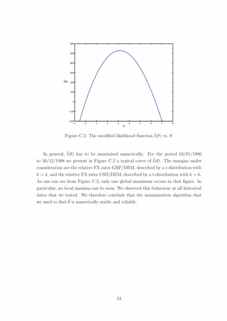
−1 0 1 2 3 4 5 6 7 8−200

−100

0

100

200

300

400

500

600

θ

~l(θ)

Figure C.2: The modified likelihood function l(θ) vs. θ.

In general, l(θ) has to be maximised numerically. For the period 02/01/1980

to 30/12/1998 we present in Figure C.2 a typical curve of l(θ). The margins under

consideration are the relative FX rates GBP/DEM, described by a t-distribution with

k = 4, and the relative FX rates USD/DEM, described by a t-distribution with k = 6.

As one can see from Figure C.2, only one global maximum occurs in that figure. In

particular, no local maxima can be seen. We observed this behaviour at all historical

dates that we tested. We therefore conclude that the maximisation algorithm that

we used to find θ is numerically stable and reliable.

53

Bibliography

[1] P. Embrechts, A. McNeil, D. Straumann, Correlation: Pitfalls and Alternatives,

RISK (May 1999), pages 69-71.

[2] P. Embrechts, A. McNeil, D. Straumann, Correlation and Dependence in Risk

Management: Properties and Pitfalls, published in Risk Management: Value at

Risk and Beyond, edited by M. Dempster, Cambridge University Press, Cam-

bridge (2002).

[3] R.B. Nelsen, An Introduction to Copulas, Springer, New York (1999).

[4] D. Duffie, J. Pan, An Overview of Value at Risk, The Journal of Derivatives, vol.

4, no. 3 (1997), pages 7-49.

[5] N.M. Zinchenko, Heavy-tailed Models in Finance and Insurance: A Survey, The-

ory of Stochastic Processes, vol. no. 1-2 (2001), pages 346-362.

[6] M.J. Frank, On the simultaneous associativity of F (x, y) and x + y − F (x, y),

Aequationes Math. 19 (1979), pages 194-226.

[7] T.P. Hutchinson, C.D. Lai, Continuous Bivariate Distributions, Emphasising

Applications, Rumsby Scientific Publishing, Adelaide (1990).

[8] Central Bank of the Federal Republic of Germany, Notes on Principle I, Part

VII, Section 34, January 2001.

[9] H.-P. Deutsch, Derivatives and Internal Models, 2nd edition, Palgrave (2002).

[10] Central Bank of the Federal Republic of Germany, Statistical Supplement “Ex-

change Rate Statistic” to the Monthly Report (January 1980 - December 1998).

[11] S. Brandt, Data Analysis, 3rd edition, Springer (1999).

[12] A. Sklar, Fonctions de repartition a n dimensions et leurs marges, Publ. Inst.

Statist. Univ. Paris 8 (1959), pages 229-231.

54

[13] A. Sklar, Random Variables, Distribution Functions, and Copulas – a Personal

Look Backward and Forward, published in Distributions with Fixed Marginals

and Related Topics, edited by L. Ruschendorf, B. Schweizer and M.D. Taylor,

Institute of Mathematical Statistics, Hayward, CA (1996), pages 1-14.

[14] J. Stoer, R. Bulirsch, Introduction to Numerical Analysis, 3rd edition, Springer

(2002).

[15] I.N. Bronshtein, K.A. Semendyayev, Handbook of Mathematics, 3rd edition,

Springer (1997).

[16] J.C. Hull, Options, Futures, and Other Derivatives, 4th edition, Prentice Hall

(2000).

55