1

Improving VANET Routing Using Visibility Regions to Avoid Communication Obstacles

Scott E. Carpenter Student Member, IEEE

Department of Computer Science North Carolina State University

Raleigh, NC, USA scarpen@ncsu.edu

In Partial Fulfillment of the Requirements of

Special Topics in Computational Geometry (CSC 591, fall, 2013), Edgar Lobaton, Ph.D.

Abstract—Wireless communications between vehicles enables both safety applications, such as accident avoidance, and

non-safety applications, such as traffic congestion alerts [1] with the intent of improving safety in driving conditions.

Broader information dissemination in vehicular ad hoc networks (VANETs) over two or more transmissions (i.e.

multihop) greatly enhances application effectiveness [2]. While many VANET-centric routing protocols exist (e.g. see [1], [2], [3], [4]), they differ in their information usage to select the next hop (e.g. state information, neighboring vehicle

position, and pre-determined street and intersection data). Especially in urban settings, obstacles, such as buildings,

foliage, and other vehicles present serious routing challenges [4] by restricting direct line of sight (LOS) communication.

Many mobile routing algorithms first allow a link to fail and then reactively enter into a route repair phase, leading to

costly communications overhead and limiting their effectiveness. Mobile network communication benefits when path

recalculations are minimized [5]. To do so, network optimization goals must achieve a viable connectivity capability while

maximizing long-term path reliability. Having only local awareness of neighbor positions is not sufficient to fully optimize

a mobile network. We propose using visibility information in next hop selection mechanisms to improve a VANET

routing capability. The overlapping visibility regions of two points represents the unobstructed zone of mutual visibility

(ZOMV) between them and motivates the following research objective: The goal of this research is to improve VANET

application effectiveness by including visibility region information proactively in the next hop node selection mechanisms of

routing protocols. The visibility-aware route connectivity route lifetime metric measures the longevity of a visibility-aware

route once it has been successfully established. As traffic density increases, the visibility-aware mechanism selects suitable

routes and, compared to the non-visibility-aware case, improves route lifetime with the hop count approaching the

optimal value. Proactively establishing viable routes reduces communications overhead that routing algorithms require

when they reactively seek alternate paths and repair failed links when obstacles restrict LOS interchanges. Reducing

communication requirements in a VANET setting reduces the possibility of transmission collisions, which in turn

enhances network reliability. A more reliable VANET information dissemination system advances application

effectiveness and promotes safety, thus supporting one of the primary goals of connected vehicle systems.

Keywords—VANET; Routing; visibility region; Zone of Mutual Visibility; minimum hop count; route lifetime;

I. INTRODUCTION

Collisions among moving vehicles lead all causes of traffic fatalities, injuries, and property damage 1 . By exchanging information using wireless communications, cars and trucks enable both safety applications, such as accident avoidance, and non-safety applications, such as traffic congestion alerts [1]. The US Intelligent Transportation Systems (ITS) Joint Program Office (JPO) suggests that vehicle safety applications and supporting technologies will prevent tens of thousands of automobile crashes every year2. The authors of [2] theorize that broader information dissemination in a vehicular ad hoc network (VANET) over two or more transmissions (i.e. multihop) greatly enhances application effectiveness. While many VANET-centric routing protocols exist (e.g. see [1], [2],[3], [4]), they differ in their information usage to select the next hop (e.g. state information, neighboring

1 National Highway Traffic Safety Administration, Fatality Analysis Reporting System (FARS) Encyclopedia, Online: [http://www-fars.nhtsa.dot.gov/Main/index.aspx], Accessed: [October 15, 2013]. 2 U.S. Department of Transportation, Connected Vehicle Research, Online: [http://www.its.dot.gov/connected_vehicle/connected_vehicle.htm], Accessed: [October 15, 2013].

2

vehicle position, and pre-determined street and intersection data). Especially in urban settings, obstacles, such as buildings, foliage, and other vehicles present serious routing challenges [4] by restricting direct line of sight (LOS) communication which cause protocols to enter a recovery stage, or fail outright, limiting their effectiveness. We propose using visibility information in next hop selecting mechanisms to improve a VANET routing capability. A visibility region describes the polygonal area from which a point has unobstructed access, or coverage. The overlapping visibility regions of two points represents the unobstructed zone of mutual visibility (ZOMV) between them and motivates the following research objective: The goal of this research is to improve VANET application effectiveness by including visibility region information proactively in the next hop node selection mechanisms of routing protocols. Our investigations are guided by the following research questions:

RQ1 Given a set of static obstacles (within a bounding region), a set of position-evolving points including starting and ending points, can mutual visibility metrics help identify a routing capability from start to finish through zero or more intermediate points?

A routing capability exists if a path exists in a routing graph from the starting point to the goal. Many routing protocols cannot realize a desired path because of communications interference on one or more links. Using visibility region information to identify a routing path which does not suffer link interference shows that such information improves routing capability. An improved routing capability makes VANET applications more effective.

RQ2 For a scenario of static obstacles how does the mobility and number of (randomly) placed points impact the route lifetime and routing capability compared to an optimal path with minimum hop count?

End-to-end application success depends upon message receipt by the next hop node in the routing path. Yet, the dynamic nature of a VANET jeopardizes the future transmission-receipt capabilities, as traffic densities change and vehicles move. A current link in the routing path may become inoperative in the future. However, the precision of ZOV boundaries supersedes that of moving vehicles contained within them. Using visibility region information within the dynamic context of a VANET improves routing capability by managing node selection and handoff before link failure.

RQ3 What is the expected complexity in time and space to select a routing path, given n points and O obstacles with a total of m vertices?

Because cars will not have supercomputers, the processing power available to them requires careful consideration. Thus, understanding the order of processing requirements for route selection mechanisms is important. In particular, we are interested in assessing time and space complexity resulting from the addition of visibility region information to routing capabilities.

Numerical simulation addresses the problem by implementing visibility region algorithms in C++ and using distance and common visibility regions between nodes for route selection. Path length and route lifetime are compared to the optimal route determined from a minimum hop count traversal of the route graph. The visibility-aware link availability metric defines the measure of link capability between nodes by combining distance and visibility region overlap, with the highest ranking value between successive pairs establishing the best link potential. Similarly, the visibility-aware path connectivity lifetime metric defines the longevity of the routing path over time. A problem space of arbitrarily static obstacles and initial start and end points establishes the baseline scenario. Parameterization of the number of randomly placed nodes, representing varying vehicle densities, culminates with the collection of statistics for route creation between the start and end points.

Our work extends the works of others by combining mutual visibility with intra-node distance for next hop selection in obstacle-rich VANET scenarios. Our contributions include:

• New metrics, the visibility-aware link availability metric and the visibility-aware connectivity lifetime metric.

• A description of Algorithm CALCULATEVISIBILITYAWAREROUTE, a route selection algorithm that incorporates visibility information and uses these new metrics.

This paper is organized as follows: Section II provides background information and discusses related works. Section III defines the problem statement formally. Section IV details the methodology. Section V describes the algorithms and their complexity analysis while Section VI discusses implementation. Section VII presents experimental results and Section VIII discusses threats to validity. Section IX concludes the paper and discusses future work.

II. BACKGROUND AND RELATED WORK

To maintain network connectivity in a VANET, direct line of sight (LOS) wireless communications is required. Yet, challenges result from the dynamic movement of vehicles. Single hop inter-vehicle communications (IVC) typically occurs within a nominal 300m range. Communications over extended ranges requires multi-hop communications, which itself requires a routing mechanism that satisfactorily addresses the LOS communications constraints. Furthermore, communications capabilities are impacted by the VANET setting. In highway settings, LOS issues most often result from roadway curvatures and blockages from large vehicles (e.g. trucks). However, in urban settings, LOS issues arise from obstacles such as buildings, foliage, and parked vehicles, and are especially prevalent at intersections with a dense surrounding of such obstacles. Regardless, a VANET routing mechanism must effectively address LOS issue for all (dynamic) environments.

3

All VANET routing protocols establish and maintain routes, yet they differ in how they query for the next hop from the set of currently reachable nodes. These differences include the number of candidate nodes to initially select, use and maintenance of link state information, reliance on prior knowledge of street-map topology, future prediction of vehicular locations, and obstacle avoidance. For successful communications, two vehicles must have an unobstructed, direct LOS view of each other. The zone of potential communications can be represented using the visibility region (or, synonymously, visibility polygon), which is the polygonal area from which a point has unobstructed access, or coverage. The direct LOS issues in a VANET make 2D polygons appropriate for the problem space. When the polygon is bounded, visibility regions often become star-shaped. The intersection of the visibility regions of two vehicles determines if both vehicles lie within a zone of mutual visibility (ZOMV), in which case both vehicles share an unobstructed, direct LOS view of one another.

VANET routing protocols need to address the challenges posed by the dynamic evolution of the network topology with the constraints of the direct LOS communications requirements. Differing in their route establishment mechanisms, VANET routing protocol classifications include: proactive, reactive, geographic, or some hybrid combination [1], [2], [3], [4]. A proactive routing protocol, such as Optimized Link State Routing (OLSR) [6] continuously maintains route information, but suffers from the communications overhead required to maintain routing tables. A reactive routing protocol, such as Ad hoc On-demand Distance Vector (AODV) [7] initiates route establishment on demand, but suffers from long setup time requirements for establishing routing tables. Proactive and reactive protocols do not use positional information and largely ignore the problem of obstacles. Geographic routing protocols, such as Greedy Perimeter Stateless Routing (GPSR) [8] use positional information of neighboring vehicles to make routing decisions, generally towards a target location, but often suffer from large packet loss.

Urban settings pose special challenges to VANET routing in that obstacles and angular approaches to traffic intersections reduce the suitability of the next hop [4]. Road geometry alone significantly impacts the throughput of VANETs [9]. Broadcast flooding is often employed to propagate data, which results in excessive data overhead. Street-aware protocols, such as Geographic Source Routing (GSR) [10] require apriori global topological street knowledge of roads. Similarly, Anchor-based Street and Traffic Aware Routing (A-STAR) [11] adds combined knowledge of junctions (e.g. intersections) and traffic awareness. While shown to significantly improve communications capabilities in urban settings, street aware protocols fail to address dynamic obstacles. Urban Multi-Hop Broadcast (UMB) [12] forwards packets without apriori topology information using broadcast flooding, but requires infrastructure to be installed at intersections. Zone Routing Protocol (ZRP) [12] selects appropriate nearby vehicles to rebroadcast messages based on their proximity within a local Zone of Relevance (ZOR), but does not use obstacle avoidance or location prediction in selecting border vehicles.

Visibility regions represent geometrically common navigation optimality problems [13] such as art gallery, motion planning, and shortest path [14]. In the polygonal area of overlapping visibility regions, two points that can see each other are mutually visible and connected by a visibility edge. Obstacle blocking has been studied using 2D polygon visibility regions, but with the goal of determining efficient locations of roadside infrastructure [9]. Homologies produced from algebraic topologies allow for navigation studies [15] and similar applications such as camera placement in sensor networks [15, 16].

When vertices represent vehicles and edges represent communications links, graph theory describes the VANET topology. Link reliability is vital in the route selection mechanism [17]. The evolving graph model, modified with VANET dynamic topology estimation [17], proposes to improve route reliability. A routing metric taxonomy is provided in [5].

We build upon the works of others by defining additional metrics in the VANET link selection process that are based on obstacle avoidance and direct LOS visibility.

III. PROBLEM STATEMENT

A. Research Goals

Effective VANET communications requires multi-hop capabilities which address the issues that arise in settings with obstacles that obstruct the direct LOS between vehicles. Yet, many routing protocols fail to directly address all LOS issues for vehicles, thus limiting routing effectiveness. For example, AODV [7] assumes local knowledge of neighbor location and uses distance vector information from all neighbors within its communications zone. AODV selects a route based on minimum hop count, where each hop is typically unit-weighted. GSPR [8], on the other hand, uses greedy forwarding and selects for the next hop the neighbor geographically closest to the ultimate destination. While AODV and GSPR both use local awareness of expected neighbor location, neither takes into account obstacle obstructions which may block LOS communications. In fact, both first allow a link to fail and then reactively enter into a route repair phase. Thus, these routing protocols often select a route which cannot be realized due to link failures, leading to costly communications overhead from identifying alternate paths.

Mobile network communication benefits when path recalculations are minimized [5]. To do so, network optimization goals must achieve a viable connectivity capability while maximizing long-term path reliability. Having only local awareness of neighbor positions is not sufficient to fully optimize a mobile network. We propose using visibility information proactively in next hop selecting mechanisms to improve a VANET routing capability. Representing the unobstructed zone of visibility (ZOV) using visibility regions motivates the following research objective: The goal of this research is improve VANET application effectiveness by including visibility region information proactively in the next hop node selection mechanisms of routing protocols. Our investigations are guided by the following research questions:

4

RQ1 Given a set of static obstacles (within a bounding region), a set of position-evolving points including starting and ending points, can mutual visibility metrics help identify a routing capability from start to finish through zero or more intermediate points?

A routing capability exists if a path exists in a routing graph from the starting point to the goal. Many routing protocols cannot realize a desired path because of communications interference on one or more links. Using visibility region information to identify a routing path which does not suffer link interference shows that such information improves routing capability. An improved routing capability makes VANET applications more effective.

RQ2 For a scenario of static obstacles how does the mobility and number of (randomly) placed points impact the route lifetime and routing capability compared to an optimal path with minimum hop count?

End-to-end application success depends upon message receipt by the next hop node in the routing path. Yet, the dynamic nature of a VANET jeopardizes the future transmission-receipt capabilities, as traffic densities change and vehicles move. A current link in the routing path may become inoperative in the future. However, the precision of ZOV boundaries supersedes that of moving vehicles contained within them. Using visibility region information within the dynamic context of a VANET improves routing capability by managing node selection and handoff before link failure.

RQ3 What is the expected complexity in time and space to select a routing path, given n points and O obstacles with a total of m vertices?

The processing power available to communicating vehicles requires consideration. Cars will not have Cray supercomputers. Thus, understanding the order of processing requirements for route select mechanisms is important. In particular, we are interested in assessing time and space complexity resulting from the addition of visibility region information to routing capabilities.

B. Model

An abstract model describes the problem context.

A 2D bounding region (i.e. an outer-most obstacle) constrains our model in which points represent vehicles and polygons represent obstacles that prevent communications. Points may move over time, but obstacles are static. Two points for which an unobstructed line can be drawn between them have communications potential. A graph represents the communications network topology in which vertices represent vehicle communications antennae and edges, weighted by a metric for communications potential, represent link availability between two neighboring nodes. If a shortest path from a starting point to a goal can be extracted from the graph, then a routing capability exists through the network. After establishing a candidate route, a mobility model affects topology and hence the route lifetime.

More formally, we frame the problem in terms of a 2D topology, which is adequate for the direct LOS communications within a VANET. In the 2-dimensional Euclidean plane, a point, p, corresponds to a certain placement of a vehicle-mounted antenna in the configuration space3. Vehicles move within the work space, avoiding a set of i obstacles, O = {O1, O2, … Oi}. The vehicle translated over a vector (x, y) is denoted as p(x, y). The configuration space of a vehicle is denoted by C(p) ∈ C, where C is the configuration space for all vehicles, which itself is further partitioned into free space, Cfree, and obstacle space, Cobstacle. Cobstacle

consists of obstacles, each of which is defined by a polygon. For simplicity, we bound C with an outer obstacle, a square. We generate a set, P, of n points (i.e. vehicles) within Cfree. Each of the pi points may or may not be mutually visible to any of the other pj points, where i≠j.

A visibility region contains the set of all points in Cfree that are visible from a point, p. A visibility region can be represented by a graph, Gp=(V, E), where V consists of the subset of visible inner vertices of Cobstacle and, additionally, intermediate points which result from extending a ray from p through inner vertices onward to intersection points with edges of Cobstacle, and E consists of the boundary segments which appropriately connect the vertices in E , dividing Cfree into the visibility region and shadow regions. That is, Gp contains the vertices, V, which defines a polygonal region with edges, E such that all points within Gp are visible from p. To test whether or not two points are mutually visible, we first construct the visibility region for every point pi∈P. A point, p, with visibility region, Vis(p), and a point, q, with visibility region, Vis(q), are mutually visible if both p and q are contained within Vis(p)∩Vis(q). For our communications model, we further restrict nearby mutually visible neighbors to those with a distance less than some threshold (e.g. 300m). That is, p and q, even though mutually visible, are assumed to be unable to communicate with one another if their separation distance is greater than such threshold.

To address the dynamicism of a VANET model, we use a simple time-varying mobility model. We assume that each (vehicle) point moves randomly and project a future position beyond time t0 for each future time step. For initial modeling, we select time steps at a rate of 60Hz. The initial trajectory vector of pi from t0 to t1 is generated randomly. This trajectory continues for subsequent time steps as long as the placement of the point remains in Cfree. If the resulting location places the mobile point in Cobstacle, the algorithm selects a different random vector that keeps the point in Cfree.

3In the 2-dimensional workspace, a vehicle would more precisely be represented as a translating and rotating polygon, having a point source transmitting and receiving antenna which would translate along with it. However, for simplicity, we use the terms vehicle and antenna synonymously, which we represent as a point source in our abstraction.

5

Given the visibility region for each vehicle, we assume global knowledge and construct another graph Gg=(V, E) in which vertices represent vehicles and edges represent the result of the communication potential between them. We test the graph for a shortest path between a starting point and a goal, and if one exists, then we say that a routing capability exists in the model.

C. Example

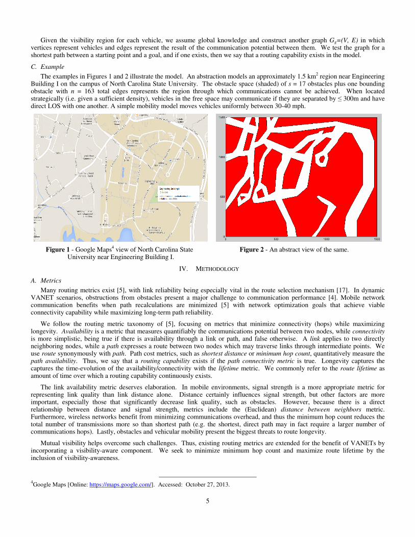
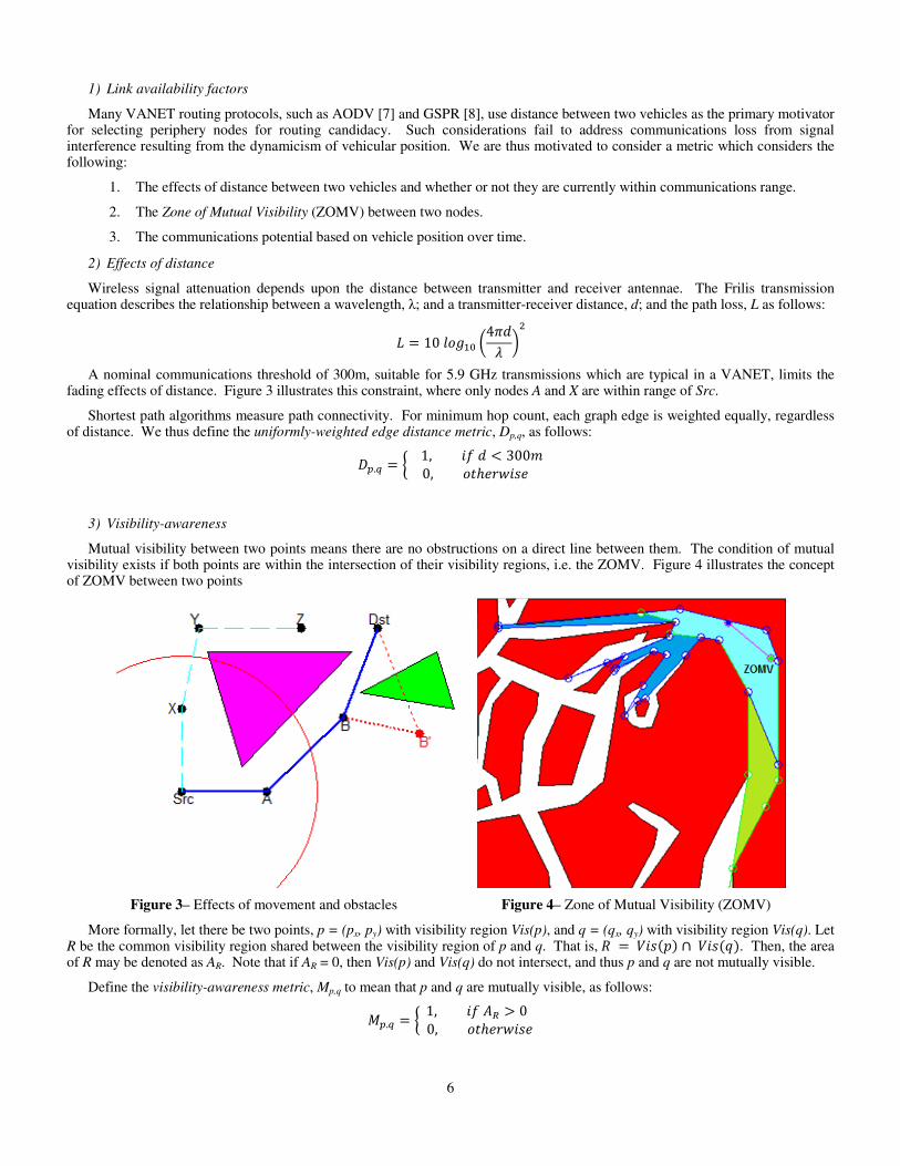
The examples in Figures 1 and 2 illustrate the model. An abstraction models an approximately 1.5 km2 region near Engineering Building I on the campus of North Carolina State University. The obstacle space (shaded) of s = 17 obstacles plus one bounding obstacle with n = 163 total edges represents the region through which communications cannot be achieved. When located strategically (i.e. given a sufficient density), vehicles in the free space may communicate if they are separated by ≤ 300m and have direct LOS with one another. A simple mobility model moves vehicles uniformly between 30-40 mph.

Figure 1 - Google Maps4 view of North Carolina State Figure 2 - An abstract view of the same. University near Engineering Building I.

IV. METHODOLOGY

A. Metrics

Many routing metrics exist [5], with link reliability being especially vital in the route selection mechanism [17]. In dynamic VANET scenarios, obstructions from obstacles present a major challenge to communication performance [4]. Mobile network communication benefits when path recalculations are minimized [5] with network optimization goals that achieve viable connectivity capability while maximizing long-term path reliability.

We follow the routing metric taxonomy of [5], focusing on metrics that minimize connectivity (hops) while maximizing longevity. Availability is a metric that measures quantifiably the communications potential between two nodes, while connectivity is more simplistic, being true if there is availability through a link or path, and false otherwise. A link applies to two directly neighboring nodes, while a path expresses a route between two nodes which may traverse links through intermediate points. We use route synonymously with path. Path cost metrics, such as shortest distance or minimum hop count, quantitatively measure the path availability. Thus, we say that a routing capability exists if the path connectivity metric is true. Longevity captures the captures the time-evolution of the availability/connectivity with the lifetime metric. We commonly refer to the route lifetime as amount of time over which a routing capability continuously exists.

The link availability metric deserves elaboration. In mobile environments, signal strength is a more appropriate metric for representing link quality than link distance alone. Distance certainly influences signal strength, but other factors are more important, especially those that significantly decrease link quality, such as obstacles. However, because there is a direct relationship between distance and signal strength, metrics include the (Euclidean) distance between neighbors metric. Furthermore, wireless networks benefit from minimizing communications overhead, and thus the minimum hop count reduces the total number of transmissions more so than shortest path (e.g. the shortest, direct path may in fact require a larger number of communications hops). Lastly, obstacles and vehicular mobility present the biggest threats to route longevity.

Mutual visibility helps overcome such challenges. Thus, existing routing metrics are extended for the benefit of VANETs by incorporating a visibility-aware component. We seek to minimize minimum hop count and maximize route lifetime by the inclusion of visibility-awareness.

4Google Maps [Online: https://maps.google.com/]. Accessed: October 27, 2013.

6

1) Link availability factors

Many VANET routing protocols, such as AODV [7] and GSPR [8], use distance between two vehicles as the primary motivator for selecting periphery nodes for routing candidacy. Such considerations fail to address communications loss from signal interference resulting from the dynamicism of vehicular position. We are thus motivated to consider a metric which considers the following:

1. The effects of distance between two vehicles and whether or not they are currently within communications range.

2. The Zone of Mutual Visibility (ZOMV) between two nodes.

3. The communications potential based on vehicle position over time.

2) Effects of distance

Wireless signal attenuation depends upon the distance between transmitter and receiver antennae. The Frilis transmission equation describes the relationship between a wavelength, λ; and a transmitter-receiver distance, d; and the path loss, L as follows:

� = 10�� �4��� ��

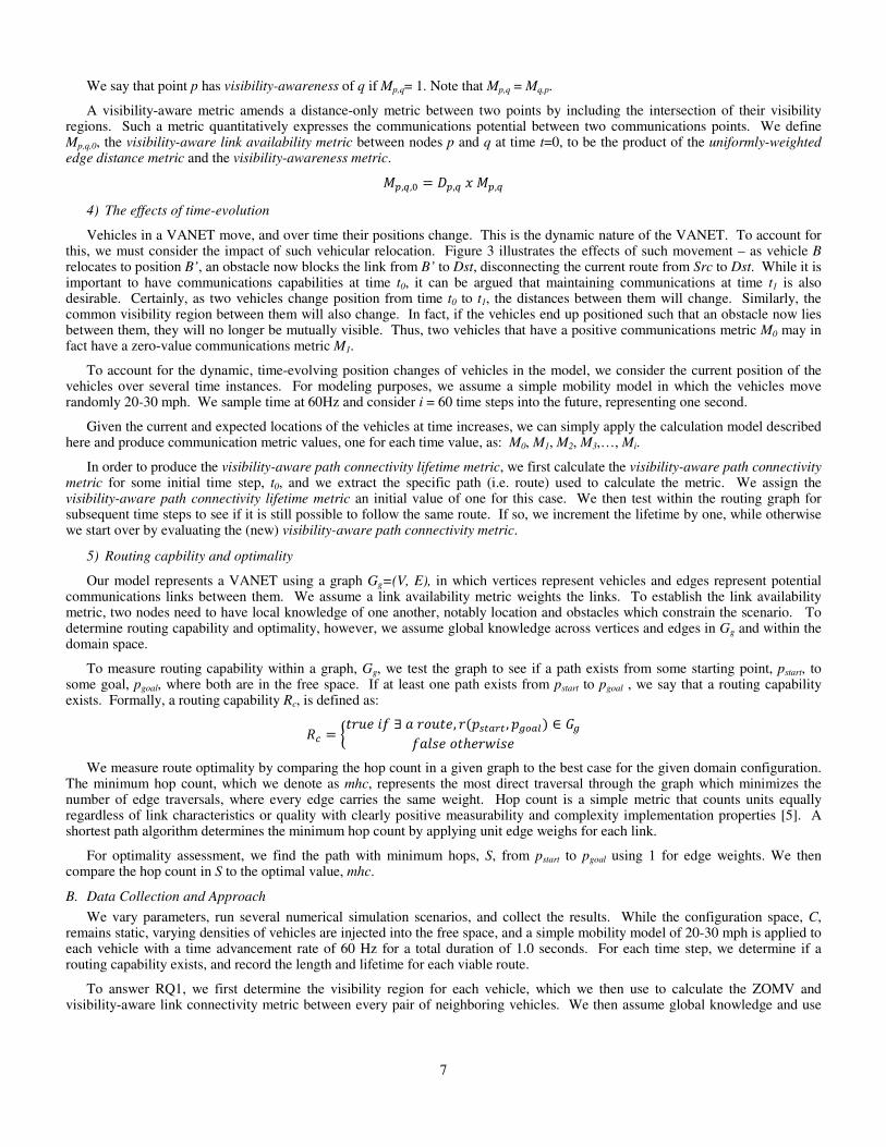
A nominal communications threshold of 300m, suitable for 5.9 GHz transmissions which are typical in a VANET, limits the fading effects of distance. Figure 3 illustrates this constraint, where only nodes A and X are within range of Src.

Shortest path algorithms measure path connectivity. For minimum hop count, each graph edge is weighted equally, regardless of distance. We thus define the uniformly-weighted edge distance metric, Dp,q, as follows:

��.� = �1, ��� < 300�0, ℎ"#$�%"

3) Visibility-awareness

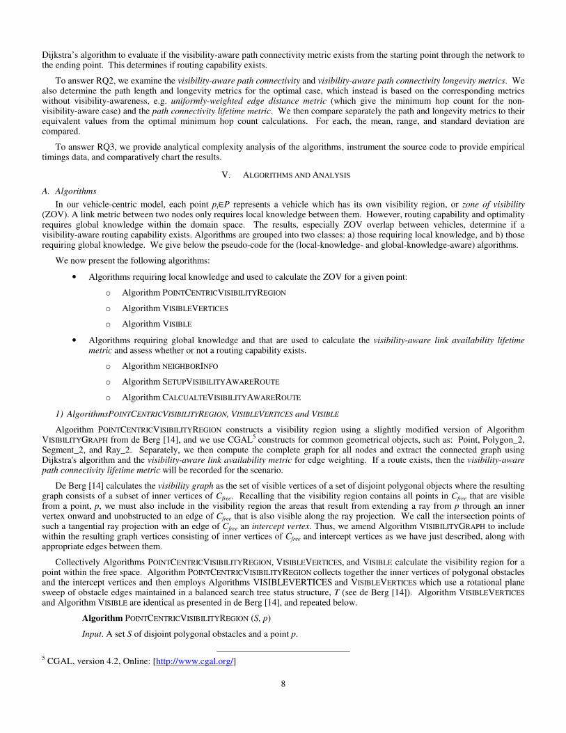
Mutual visibility between two points means there are no obstructions on a direct line between them. The condition of mutual visibility exists if both points are within the intersection of their visibility regions, i.e. the ZOMV. Figure 4 illustrates the concept of ZOMV between two points

Figure 3– Effects of movement and obstacles Figure 4– Zone of Mutual Visibility (ZOMV)

More formally, let there be two points, p = (px, py) with visibility region Vis(p), and q = (qx, qy) with visibility region Vis(q). Let R be the common visibility region shared between the visibility region of p and q. That is, & = '�%()* ∩ '�%(+*. Then, the area of R may be denoted as AR. Note that if AR = 0, then Vis(p) and Vis(q) do not intersect, and thus p and q are not mutually visible.

Define the visibility-awareness metric, Mp,q to mean that p and q are mutually visible, as follows:

,�.� = � 1, ��-. > 00, ℎ"#$�%"

7

We say that point p has visibility-awareness of q if Mp,q= 1. Note that Mp,q = Mq,p.

A visibility-aware metric amends a distance-only metric between two points by including the intersection of their visibility regions. Such a metric quantitatively expresses the communications potential between two communications points. We define Mp,q,0, the visibility-aware link availability metric between nodes p and q at time t=0, to be the product of the uniformly-weighted edge distance metric and the visibility-awareness metric.

,�,�, = ��,� 0,�,�

4) The effects of time-evolution

Vehicles in a VANET move, and over time their positions change. This is the dynamic nature of the VANET. To account for this, we must consider the impact of such vehicular relocation. Figure 3 illustrates the effects of such movement – as vehicle B relocates to position B’, an obstacle now blocks the link from B’ to Dst, disconnecting the current route from Src to Dst. While it is important to have communications capabilities at time t0, it can be argued that maintaining communications at time t1 is also desirable. Certainly, as two vehicles change position from time t0 to t1, the distances between them will change. Similarly, the common visibility region between them will also change. In fact, if the vehicles end up positioned such that an obstacle now lies between them, they will no longer be mutually visible. Thus, two vehicles that have a positive communications metric M0 may in fact have a zero-value communications metric M1.

To account for the dynamic, time-evolving position changes of vehicles in the model, we consider the current position of the vehicles over several time instances. For modeling purposes, we assume a simple mobility model in which the vehicles move randomly 20-30 mph. We sample time at 60Hz and consider i = 60 time steps into the future, representing one second.

Given the current and expected locations of the vehicles at time increases, we can simply apply the calculation model described here and produce communication metric values, one for each time value, as: M0, M1, M2, M3,…, Mi.

In order to produce the visibility-aware path connectivity lifetime metric, we first calculate the visibility-aware path connectivity metric for some initial time step, t0, and we extract the specific path (i.e. route) used to calculate the metric. We assign the visibility-aware path connectivity lifetime metric an initial value of one for this case. We then test within the routing graph for subsequent time steps to see if it is still possible to follow the same route. If so, we increment the lifetime by one, while otherwise we start over by evaluating the (new) visibility-aware path connectivity metric.

5) Routing capbility and optimality

Our model represents a VANET using a graph Gg=(V, E), in which vertices represent vehicles and edges represent potential communications links between them. We assume a link availability metric weights the links. To establish the link availability metric, two nodes need to have local knowledge of one another, notably location and obstacles which constrain the scenario. To determine routing capability and optimality, however, we assume global knowledge across vertices and edges in Gg and within the domain space.

To measure routing capability within a graph, Gg, we test the graph to see if a path exists from some starting point, pstart, to some goal, pgoal, where both are in the free space. If at least one path exists from pstart to pgoal , we say that a routing capability exists. Formally, a routing capability Rc, is defined as:

&1 = � #2"��∃4#2 ", #()56786 , )9:7;* ∈ <9�4%" ℎ"#$�%"

We measure route optimality by comparing the hop count in a given graph to the best case for the given domain configuration. The minimum hop count, which we denote as mhc, represents the most direct traversal through the graph which minimizes the number of edge traversals, where every edge carries the same weight. Hop count is a simple metric that counts units equally regardless of link characteristics or quality with clearly positive measurability and complexity implementation properties [5]. A shortest path algorithm determines the minimum hop count by applying unit edge weighs for each link.

For optimality assessment, we find the path with minimum hops, S, from pstart to pgoal using 1 for edge weights. We then compare the hop count in S to the optimal value, mhc.

B. Data Collection and Approach

We vary parameters, run several numerical simulation scenarios, and collect the results. While the configuration space, C, remains static, varying densities of vehicles are injected into the free space, and a simple mobility model of 20-30 mph is applied to each vehicle with a time advancement rate of 60 Hz for a total duration of 1.0 seconds. For each time step, we determine if a routing capability exists, and record the length and lifetime for each viable route.

To answer RQ1, we first determine the visibility region for each vehicle, which we then use to calculate the ZOMV and visibility-aware link connectivity metric between every pair of neighboring vehicles. We then assume global knowledge and use

8

Dijkstra’s algorithm to evaluate if the visibility-aware path connectivity metric exists from the starting point through the network to the ending point. This determines if routing capability exists.

To answer RQ2, we examine the visibility-aware path connectivity and visibility-aware path connectivity longevity metrics. We also determine the path length and longevity metrics for the optimal case, which instead is based on the corresponding metrics without visibility-awareness, e.g. uniformly-weighted edge distance metric (which give the minimum hop count for the non-visibility-aware case) and the path connectivity lifetime metric. We then compare separately the path and longevity metrics to their equivalent values from the optimal minimum hop count calculations. For each, the mean, range, and standard deviation are compared.

To answer RQ3, we provide analytical complexity analysis of the algorithms, instrument the source code to provide empirical timings data, and comparatively chart the results.

V. ALGORITHMS AND ANALYSIS

A. Algorithms

In our vehicle-centric model, each point pi∈P represents a vehicle which has its own visibility region, or zone of visibility (ZOV). A link metric between two nodes only requires local knowledge between them. However, routing capability and optimality requires global knowledge within the domain space. The results, especially ZOV overlap between vehicles, determine if a visibility-aware routing capability exists. Algorithms are grouped into two classes: a) those requiring local knowledge, and b) those requiring global knowledge. We give below the pseudo-code for the (local-knowledge- and global-knowledge-aware) algorithms.

We now present the following algorithms:

• Algorithms requiring local knowledge and used to calculate the ZOV for a given point:

o Algorithm POINTCENTRICVISIBILITYREGION

o Algorithm VISIBLEVERTICES

o Algorithm VISIBLE

• Algorithms requiring global knowledge and that are used to calculate the visibility-aware link availability lifetime metric and assess whether or not a routing capability exists.

o Algorithm NEIGHBORINFO

o Algorithm SETUPVISIBILITYAWAREROUTE

o Algorithm CALCUALTEVISIBILITYAWAREROUTE

1) AlgorithmsPOINTCENTRICVISIBILITYREGION, VISIBLEVERTICES and VISIBLE

Algorithm POINTCENTRICVISIBILITYREGION constructs a visibility region using a slightly modified version of Algorithm VISIBILITYGRAPH from de Berg [14], and we use CGAL5 constructs for common geometrical objects, such as: Point, Polygon_2, Segment_2, and Ray_2. Separately, we then compute the complete graph for all nodes and extract the connected graph using Dijkstra's algorithm and the visibility-aware link availability metric for edge weighting. If a route exists, then the visibility-aware path connectivity lifetime metric will be recorded for the scenario.

De Berg [14] calculates the visibility graph as the set of visible vertices of a set of disjoint polygonal objects where the resulting graph consists of a subset of inner vertices of Cfree. Recalling that the visibility region contains all points in Cfree that are visible from a point, p, we must also include in the visibility region the areas that result from extending a ray from p through an inner vertex onward and unobstructed to an edge of Cfree that is also visible along the ray projection. We call the intersection points of such a tangential ray projection with an edge of Cfree an intercept vertex. Thus, we amend Algorithm VISIBILITYGRAPH to include within the resulting graph vertices consisting of inner vertices of Cfree and intercept vertices as we have just described, along with appropriate edges between them.

Collectively Algorithms POINTCENTRICVISIBILITYREGION, VISIBLEVERTICES, and VISIBLE calculate the visibility region for a point within the free space. Algorithm POINTCENTRICVISIBILITYREGION collects together the inner vertices of polygonal obstacles and the intercept vertices and then employs Algorithms VISIBLEVERTICES and VISIBLEVERTICES which use a rotational plane sweep of obstacle edges maintained in a balanced search tree status structure, T (see de Berg [14]). Algorithm VISIBLEVERTICES and Algorithm VISIBLE are identical as presented in de Berg [14], and repeated below.

Algorithm POINTCENTRICVISIBILITYREGION (S, p)

Input. A set S of disjoint polygonal obstacles and a point p.

5 CGAL, version 4.2, Online: [http://www.cgal.org/]

9

Output. A graph, Gvis(S), representing the visibility region.

1. Initialize a graph G = (V,E) where V is the set of all (inner) vertices of thepolygons in S and E = ∅.

2. For every vertex v ∈V, project a ray, r, from v through each endpoint, si, of each edge ej∈E, and add to Vany resulting intersection points of r and every other edge ek∈E; j ≠ >.

3. W←VISIBLEVERTICES(p,S)

4. For every vertex w∈W, add the arc (p,w) to E.

5. return G.

Algorithm VISIBLEVERTICES(p, S)

Input. A set S of polygonal obstacles and a point p that does not lie in the interior of any obstacle.

Output. The set of all obstacle vertices visible from p.

1. Sort the obstacle vertices according to the clockwise angle that the half-line from p to each vertex makes with the positive x-axis. In case of ties, vertices closer to p should come before vertices farther from p. Let w1, . . . ,wn be the sorted list.

2. Let ρ be the half-line parallel to the positive x-axis starting at p. Find the obstacle edges that are properly intersected by ρ, and store them in a balanced search tree T in the order in which they are intersected by ρ.

3. W←∅

4. for i←1 to n

5. do if VISIBLE(wi) then Add wi toW.

6. Insert into T the obstacle edges incident to wi that lie on the clockwiseside of the half-line from p to wi.

7. Delete from T the obstacle edges incident to wi that lie on thecounterclockwise side of the half-line from p to wi.

8. returnW

Algorithm VISIBLE(wi)

1. if)$?@@@@@ intersects the interior of the obstacle of which wi is a vertex, locally at wi

3. ` else if i = 1 orwi−1 is not on the segment )$?@@@@@

4. then Search in T for the edge e in the leftmost leaf.

5. if e exists and )$?@@@@@intersects e

6. then return false

7. else return true

8. else if wi−1 is not visible

9. then return false

10. else Search in T for an edge e that intersects $?A�$?@@@@@@@@@.

11. if e exists

12. then return false

13. else return true

Theorem 1: The visibility region for a point. p, in a free space Cfree of a set S of disjoint polygonal obstacles, Cobstacle, with n edges in total can be computed in O(n2 log n) time.

Proof. In VISIBLEVERTICES, line 1 sorts the vertices in cyclic order around p in time complexity O(nlogn) and eclipses the time ahead of the loop. For each of the n edges in S, one execution of the loop then involves a constant number of operations on the

10

balanced search tree T, which take O(logn) time each, plus a constant number of geometric tests that take each constant time. Hence, one execution takes O(logn) time, leading to an overall running time of O(nlogn).

To compute the entire visibility region, we apply VISIBLEVERTICES to each of the n original inner vertices of S plus the intercept points found in line 2 of POINTCENTRICVISIBILITYREGION. There is at most one intercept point for each edge in S, and there are O(n) edges in S, giving at most O(n) additional intercept points. Finding each intercept point can be done in O(1) time, so line 2 is bound by O(n) time. Together, line 1 and line 2 add O(n) total vertices to V, and we have stated that each execution of VISIBLEVERTICES takes O(nlogn) time. Overall, we get the following: The visibility region for a point p in a free space bound by a set S of disjoint polygonal obstacles with n edges in total can be computed in O(n2 logn) time.

We now examine empirically timing results as compared to our analytical expectations. Recall that in our configuration space that obstacles are fixed and some number of points, m, are randomly placed in the free space with simple mobility applied over t – 1 further time steps (for a total of t placements).Thus, we generate the visibility region for each of m x t points. But, the number of edges, n, is fixed, so we expect the time to calculate the visibility region for each of the mt points to be constant O(n2 logn). We wish to show two things, which we address separately. First, we vary the number of obstacle vertices, n, to show that our algorithm follows the expected time complexity as n varies. Second, we then show that our algorithm applied to a fixed obstacle space calculates visibility regions in nearly constant time as the total number of algorithm invocations increases with mt, the vehicle density and time steps.

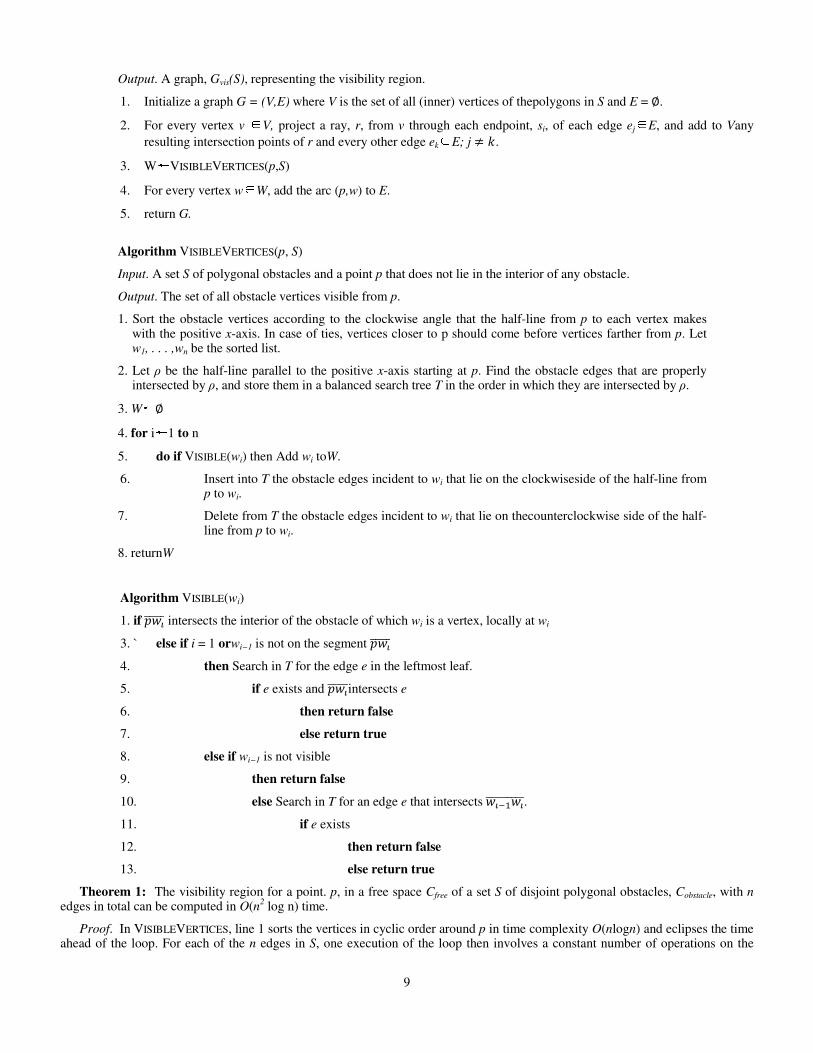
To show the impact to time as obstacle vertices increase, we conduct an experiment where we generate a random number of disjoint polygonal obstacles, with increasing number of edges per obstacle. We instrument Algorithm VISIBILITYREGION to record the time to calculate the visibility region for n obstacle vertices, and conduct several trials. Figure 5 charts the expected (i.e. analytical) results and the empirical (i.e. instrumented) results of three identical trials of increasing n. We observe two things in the results. First, each of three separate empirical trials is presented. The results should be identical, as the random number generator seed used in each trial was the same. However, some minor variation between the trials is clearly noticeable. Second, despite the variation between trials, we also see that the trends of each generally follow the analytical (i.e. expected) time complexity results, which as n varies, should be O(n2 logn). Note that we have adjusted the expected analytical results (i.e. n2 logn) by a scaling factor (e.g. 1/2000) to make the time scale (i.e. y-axis) consistent.

0

50

100

150

200

250

300

350

400

125 175 225 275

Tim

e,

ms

Number of obstacle vertices

Algorithm VisibilityRegionTimings - Expected vs. Empirical

Expected(analytical)

Empirical(trial 1)

Empirical(trial 2)

Empirical(trial 3)

Figure 5 – Time complexity for Algorithm VISIBILITYREGION

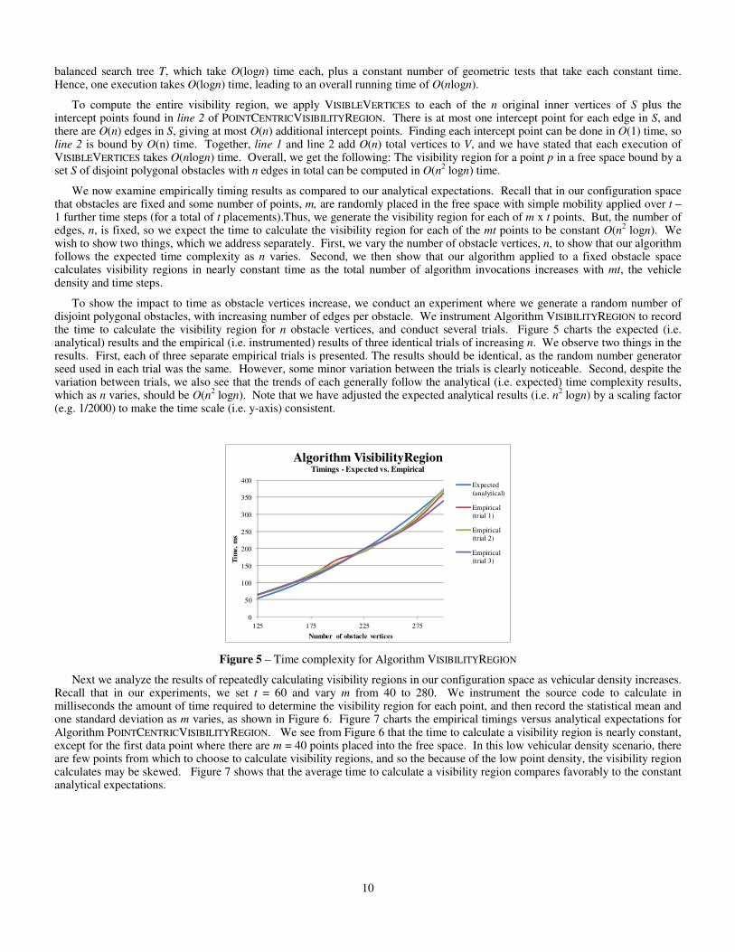
Next we analyze the results of repeatedly calculating visibility regions in our configuration space as vehicular density increases. Recall that in our experiments, we set t = 60 and vary m from 40 to 280. We instrument the source code to calculate in milliseconds the amount of time required to determine the visibility region for each point, and then record the statistical mean and one standard deviation as m varies, as shown in Figure 6. Figure 7 charts the empirical timings versus analytical expectations for Algorithm POINTCENTRICVISIBILITYREGION. We see from Figure 6 that the time to calculate a visibility region is nearly constant, except for the first data point where there are m = 40 points placed into the free space. In this low vehicular density scenario, there are few points from which to choose to calculate visibility regions, and so the because of the low point density, the visibility region calculates may be skewed. Figure 7 shows that the average time to calculate a visibility region compares favorably to the constant analytical expectations.

11

100

120

140

160

180

200

220

240

260

280

300

2400 4800 7200 9600 12000 14400 16800

Instr

um

en

ted

tim

e,

ms

mt = number of times to calculate visibility region

Algorithm PointCentricVisibilityRegionTime Complexity, mean +/- σ

Mean

40000

45000

50000

55000

60000

65000

70000

100

120

140

160

180

200

220

240

260

280

300

2400 4800 7200 9600 12000 14400 16800

tim

e,

ms

mt = number of times to calculate visibility region

Algorithm PointCentricVisibilityRegionTime Complexity, empirical vs. analytical

Empirical(instrumented sourcecode)

Analytical,O(n^2logn),n=163

Figure 6 – Time complexity for Figure 7 – Empirical vs. expected time complexity Algorithm POINTCENTRICVISIBILITYREGION for Algorithm POINTCENTRICVISIBILITYREGION

2) Algorithm NEIGHBORINFO

Algorithm NEIGHBORINFO populates the distance and overlapping visibility regions between every pair of node from a set of visibility regions, SGvis.

Algorithm NEIGHBORINFO(SGvis)

Input. A set,SGvis, of visibility regions for each point pi∈P.

Output.A structure N, of the route data between each pair of points pi, pj, ∈P; i≠j.

1. for i = 1 to |SGvis |

2. for j = 1 to | SGvis |

3. if i≠j

4. then N[i][j].dist = Euclidean distance between pi, pj

5. N[i][j].overlapArea = the area of SGvis[i] ∩SGvis[j]

6. else N[i][j].dist = 0

7. N[i][j].overlapArea = 0

8. return N

Theorem 2: The route data between every pair of m points in the free space can be computed in O(m2(vlogv + klogk)) expected time, where v is the expected total vertices and k is the expected complexity in the intersection of any two visibility regions.

Proof. The route data includes the Euclidean distance between the two neighboring points (i.e. line 4), which can be calculated in O(1) time, and the ZOMV, which is the area of the overlapping visibility regions of the two neighboring points (i.e. line 5). A polygonal Boolean operation calculates the intersection of two polygons with v total vertices and output complexity k in O(vlogv + klogk) time [14], which therefore bounds lines 3 – 7, which are executed by line 1 and line 2 a total of m2 times. Thus, the route data for m points in a free space where a pair of neighboring points has expected v total vertices and k complexity in the intersection of their visibility regions is bounded in time by O(m2(vlogv + klogk)).

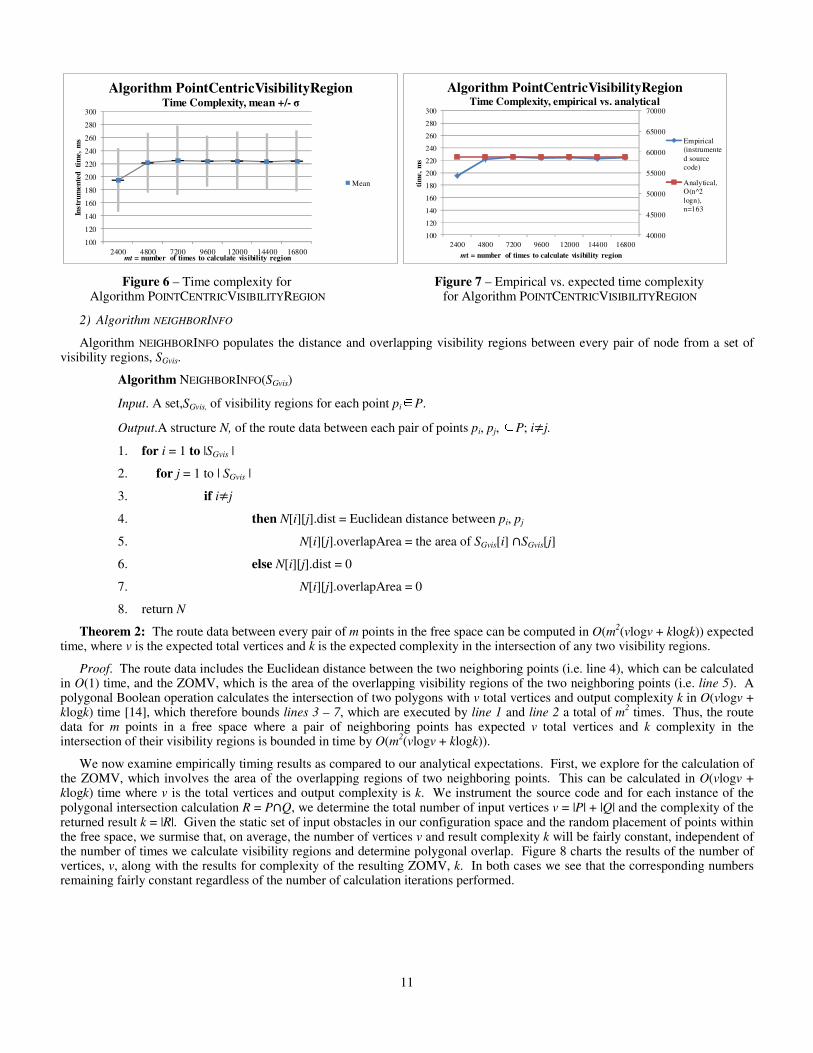
We now examine empirically timing results as compared to our analytical expectations. First, we explore for the calculation of the ZOMV, which involves the area of the overlapping regions of two neighboring points. This can be calculated in O(vlogv + klogk) time where v is the total vertices and output complexity is k. We instrument the source code and for each instance of the polygonal intersection calculation R = P∩Q, we determine the total number of input vertices v = |P| + |Q| and the complexity of the returned result k = |R|. Given the static set of input obstacles in our configuration space and the random placement of points within the free space, we surmise that, on average, the number of vertices v and result complexity k will be fairly constant, independent of the number of times we calculate visibility regions and determine polygonal overlap. Figure 8 charts the results of the number of vertices, v, along with the results for complexity of the resulting ZOMV, k. In both cases we see that the corresponding numbers remaining fairly constant regardless of the number of calculation iterations performed.

12

0

5

10

15

20

25

30

35

1600 6400 14400 25600 40000 57600 78400

nu

mber

of

verti

ces

m^2 = number of times to calculate polygonal intersection

Polygonal Intersectionv and k vs. number of calculations

v = totalvertices of P, Q

k = complexityof intersectionof P, Q

0

1000

2000

3000

4000

5000

6000

7000

8000

0

10000

20000

30000

40000

50000

60000

70000

80000

90000

40 80 120 160 200 240 280

tim

e,

ms

m = number of points in free space

Algorithm NeighborInfoTime complexity

Analytical(expected),m^2

Empiricaltimings

Figure 8 – Values of v and k are generally constant Figure 9 – Time complexity of Algorithm NEIGHBORINFO and independent of the number of polygonal intersections calculated

We next examine the time to calculate the neighbor information using Algorithm NEIGHBORINFO,, which we do by instrumenting the code to record the timing for each execution of the algorithm, which we compare to analytical (i.e. expected) results. As we note, the values of v and k are nearly constant in our experiments, so we treat the terms vlogv + klogk) as constant, and thus we expect to see the timings to be dependent on m2. Figure 9 charts our results, which shows this trend.

3) AlgorithmsSETUPVISIBILITYAWAREROUTE and CALCUALTEVISIBILITYAWAREROUTE

The primary calculation algorithm includes a preprocessing step, SETUPVISIBILITYAWAREROUTE that exists solely to set up the configuration space and which we thus exclude from complexity analysis. Algorithm CALCULATEVISIBILITYAWAREROUTE

consists of three main steps. The first step calculates all the visibility regions for every point and the second step computes neighbor information between each pair of points. Using the neighbor information, the remainder of the algorithm creates a graph with edge weightings based on either a non-visibility awareness metric (i.e. to give the optimal minimum hop count), or one based on the visibility-awareness link connectivity metric (i.e. for comparison to the optimal routing path). The final step evaluates routing capability using Dijkstra’s algorithm and compares and reports results.

Algorithm SETUPVISIBILITYAWAREROUTE(n, s, m, f)

Input. The number of points to be created in the freespace, n, the number of 60 Hz times steps, s, and the range, m + [0, f), over which each point moves each time step.

Output. An established configuration space, C, consisting of a set S of disjoint polygonal obstacles, and an array of sets, P[s], of starting and ending points, Pstart and Pgoal and randomly-placed points in the free space.

1. S = ∅. P[1..s] = ∅.

2. Add a boundary obstacle (i.e. 1500 m x 1500 m rectangular box) to S.

3. Create static obstacles and add each to S.

4. for t = 1..s, do

5. Add Pstart and Pgoal to P[t].

6. for i = 1..n, do

7. Create randomly placed points in the free space and their subsequent s locations using a simple mobility model which move each point m + [0, f) during each time step, and add each point to P[t].

Algorithm CALCUALTEVISIBILITYAWAREROUTE(C, s)

Input. An established configuration space, C, created by Algorithm SETUPVISIBILITYAWAREROUTE and the number of time steps, s.

Output. Visibility-aware and non-visibility-aware route connectivity and longevity results.

1. for each time step t = 1..s, do

2. for each point p ∈ P[t], do

13

3. Calculate the visibility region for p using Algorithm POINTCENTRICVISIBILITYREGION and store the results in a structure, VR[t]

4. for each time step t = 1..s, do

5. N = NEIGHBORINFO(VR[t])

6. for each metric m ∈ {minimum hop count, visibility-aware minimum hop count} do

7. for each time stept = 1..s, do

8. for each pair of points pi ∈ P[t], pj ∈ P[t], i ≠j, do

9. Calculate the appropriate visibility-aware link availability or uniformly-weighted edge distance metric (i.e. as appropriate depending on m)

10. Construct a graph, Gg, from all points in the free space with edge weight using the metric calculated above.

11. Use Dijkstra’s algorithm to determine the best route, R, within Gg, from Pstart to Pgoal (i.e. the minimum hop count shortest path).

12. Evaluate if R is actually viable (i.e. obstacles do not block communications)

13. Record in a vector the path length, and route longevity

14. Report the metric type, path lengths and their mean, range, and standard deviation; and the route lifetimes and their mean, range, and standard deviation.

Theorem 3: The visibility-aware routing over t time steps for m points in the free space of a set S of polygonal obstacles with n total edges can be computed in O(mt(n

2logn + m(vlogv + klogk))) expected time, where v is the expected total vertices and k is the expected complexity in the intersection of any two visibility regions (i.e. visibility polygons).

Proof. As already stated, Algorithm CALCULATEVISIBILITYAWAREROUTE consists of three main steps which calculates all the visibility regions for every point, computes neighbor information between each pair of points, and evaluates routing capability using Dijkstra’s algorithm and compares and reports results. The visibility regions for all points utilizes Algorithm POINTCENTRICVISIBILITYREGION on line 3, which we have already proven by Theorem 1 to take O(n2 logn) time to calculate the visibility region for one point. Line 1 and line 2 execute this for m points over t time steps, so the overall time complexity to calculate all visibility regions is O(mtn

2logn). We have also already shown by Theorem 2 that Algorithm NEIGHBORINFO calculates the route data between every pair of m points in the free space in time complexity O(m2(vlogv + klogk)). Line 4 executes this in t time steps, so the total time complexity of the second step is O(tm2(vlogv + klogk)). The edge-weighting metric calculation occurs on line 9, which retrieves from N the Euclidean distance between two points in the case of the uniformly-weighted edge distance metric and, additionally, the area of the ZOMV in the case of the visibility-aware link availability metric. Since both were previously computed in the NEIGHBORINFO step, retrieval from N in line 9 takes O(1). Since line 8 executes line 9 a total of m2

times, the total time complexity for line 8 and line 9 is O(m2). The graph, Gg=(V, E), is constructed in line 10 by adding all m points to V and examining the pairwise information in N to add the potential edges to E. Since the complexity of N is m2, such examination takes O(m2) time, and bounds the step. Line 11 uses Dijkstra’s algorithm to compute the shortest path from pstart to pgoal through graph Gg, which, for m nodes and o arcs between them can be calculated in O(mlogm + o) time [14]. Line 12 evaluates the route returned from line 11 by traversing the route and examining the connectivity metrics in N. Since the route length is O(m), and the connectivity metrics for the link between each successive node can be retrieved from N in O(1) time, the total time complexity for line 12 is O(m). Line 13 is clearly O(1). Hence, lines 8 – 13 are time bound by O(m2) and are executed t times (plus once for each of two metrics), for a total time complexity of O(m2

t). Finally, line 14 calculates the statistics for the collection of routes and is bound by the number of routes in the collection, which is no more than t. The overall time complexity of Algorithm CALCULATEVISIBILITYAWAREROUTE is therefore bound by O(mtn

2logn +tm2(vlogv + klogk) + m2

t) which reduces to O(mt(n

2logn + m(vlogv + klogk))).

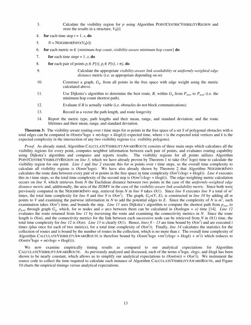
We now examine empirically timing results as compared to our analytical expectations for Algorithm CALCULATEVISIBILITYAWAREROUTE. As previously analyzed and discussed, each of the terms n2logn, vlogv, and klogk has been shown to be nearly constant, which allows us to simplify our analytical expectations to O(mt(m)) = O(m2

t). We instrument the source code to collect the time required to calculate each instance of Algorithm CALCULATEVISIBILITYAWAREROUTE, and Figure 10 charts the empirical timings versus analytical expectations.

14

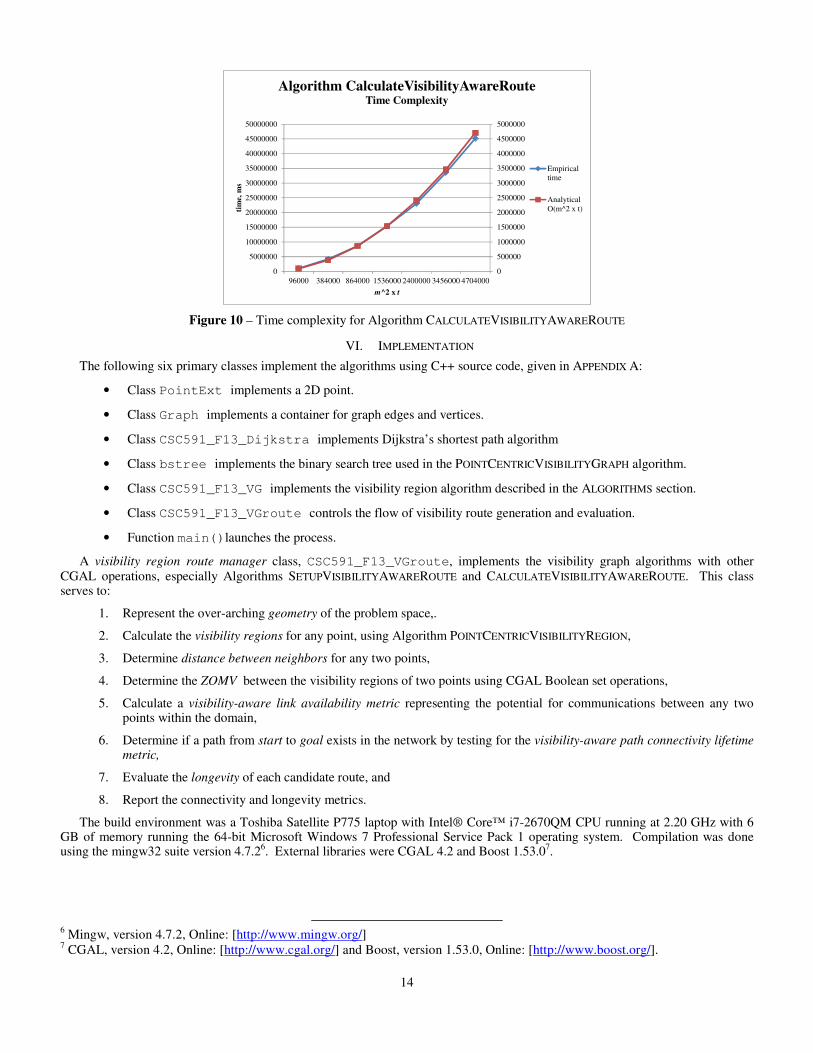
Figure 10 – Time complexity for Algorithm CALCULATEVISIBILITYAWAREROUTE

VI. IMPLEMENTATION

The following six primary classes implement the algorithms using C++ source code, given in APPENDIX A:

• Class PointExt implements a 2D point.

• Class Graph implements a container for graph edges and vertices.

• Class CSC591_F13_Dijkstra implements Dijkstra’s shortest path algorithm

• Class bstree implements the binary search tree used in the POINTCENTRICVISIBILITYGRAPH algorithm.

• Class CSC591_F13_VG implements the visibility region algorithm described in the ALGORITHMS section.

• Class CSC591_F13_VGroute controls the flow of visibility route generation and evaluation.

• Function main()launches the process.

A visibility region route manager class, CSC591_F13_VGroute, implements the visibility graph algorithms with other CGAL operations, especially Algorithms SETUPVISIBILITYAWAREROUTE and CALCULATEVISIBILITYAWAREROUTE. This class serves to:

1. Represent the over-arching geometry of the problem space,.

2. Calculate the visibility regions for any point, using Algorithm POINTCENTRICVISIBILITYREGION,

3. Determine distance between neighbors for any two points,

4. Determine the ZOMV between the visibility regions of two points using CGAL Boolean set operations,

5. Calculate a visibility-aware link availability metric representing the potential for communications between any two points within the domain,

6. Determine if a path from start to goal exists in the network by testing for the visibility-aware path connectivity lifetime metric,

7. Evaluate the longevity of each candidate route, and

8. Report the connectivity and longevity metrics.

The build environment was a Toshiba Satellite P775 laptop with Intel® Core™ i7-2670QM CPU running at 2.20 GHz with 6 GB of memory running the 64-bit Microsoft Windows 7 Professional Service Pack 1 operating system. Compilation was done using the mingw32 suite version 4.7.26. External libraries were CGAL 4.2 and Boost 1.53.07.

6 Mingw, version 4.7.2, Online: [http://www.mingw.org/] 7 CGAL, version 4.2, Online: [http://www.cgal.org/] and Boost, version 1.53.0, Online: [http://www.boost.org/].

0

500000

1000000

1500000

2000000

2500000

3000000

3500000

4000000

4500000

5000000

0

5000000

10000000

15000000

20000000

25000000

30000000

35000000

40000000

45000000

50000000

96000 384000 864000 1536000 2400000 3456000 4704000

tim

e, m

s

m^2 x t

Algorithm CalculateVisibilityAwareRouteTime Complexity

Empiricaltime

AnalyticalO(m^2 x t)

15

VII. EXPERIMENTAL VALIDATION

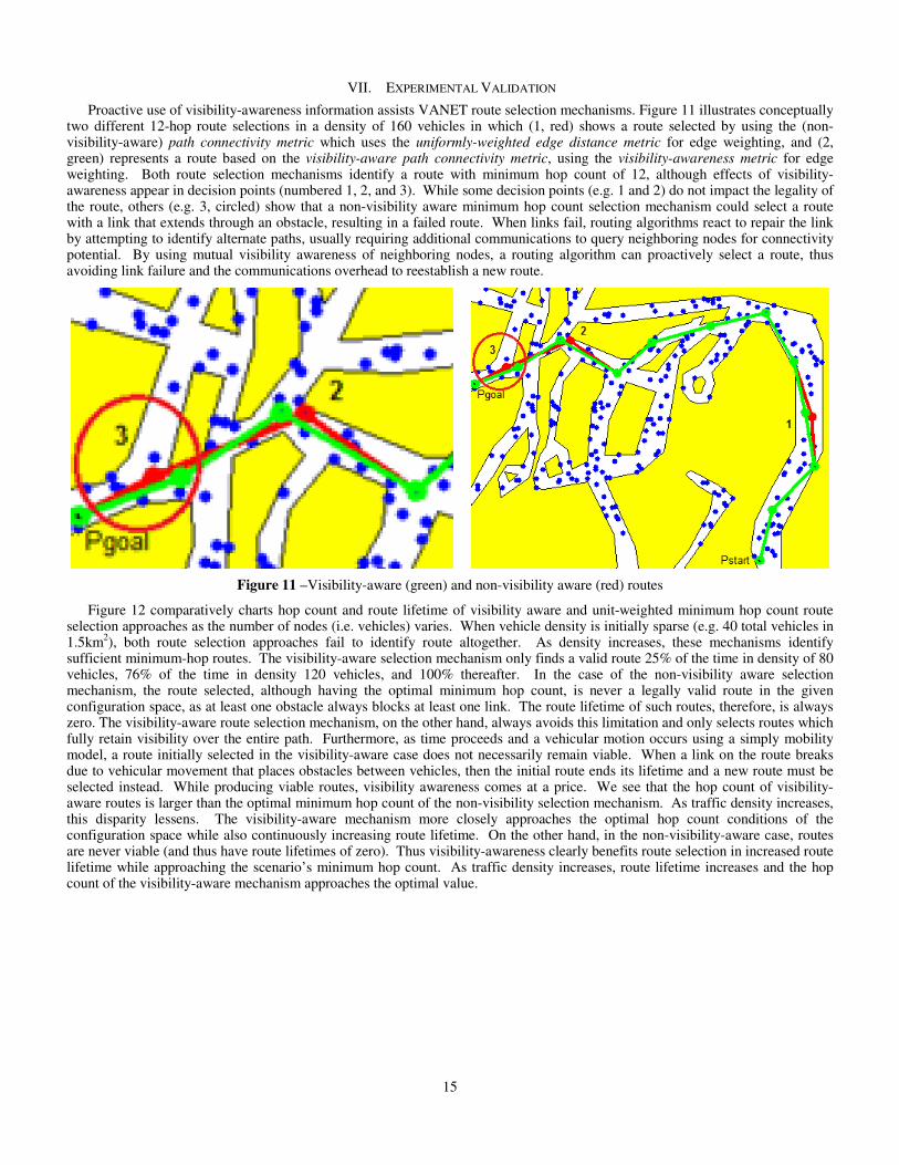
Proactive use of visibility-awareness information assists VANET route selection mechanisms. Figure 11 illustrates conceptually two different 12-hop route selections in a density of 160 vehicles in which (1, red) shows a route selected by using the (non-visibility-aware) path connectivity metric which uses the uniformly-weighted edge distance metric for edge weighting, and (2, green) represents a route based on the visibility-aware path connectivity metric, using the visibility-awareness metric for edge weighting. Both route selection mechanisms identify a route with minimum hop count of 12, although effects of visibility-awareness appear in decision points (numbered 1, 2, and 3). While some decision points (e.g. 1 and 2) do not impact the legality of the route, others (e.g. 3, circled) show that a non-visibility aware minimum hop count selection mechanism could select a route with a link that extends through an obstacle, resulting in a failed route. When links fail, routing algorithms react to repair the link by attempting to identify alternate paths, usually requiring additional communications to query neighboring nodes for connectivity potential. By using mutual visibility awareness of neighboring nodes, a routing algorithm can proactively select a route, thus avoiding link failure and the communications overhead to reestablish a new route.

Figure 11 –Visibility-aware (green) and non-visibility aware (red) routes

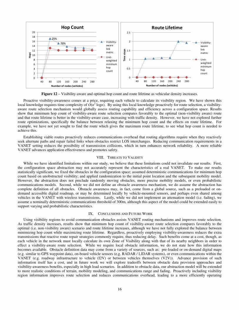
Figure 12 comparatively charts hop count and route lifetime of visibility aware and unit-weighted minimum hop count route selection approaches as the number of nodes (i.e. vehicles) varies. When vehicle density is initially sparse (e.g. 40 total vehicles in 1.5km2), both route selection approaches fail to identify route altogether. As density increases, these mechanisms identify sufficient minimum-hop routes. The visibility-aware selection mechanism only finds a valid route 25% of the time in density of 80 vehicles, 76% of the time in density 120 vehicles, and 100% thereafter. In the case of the non-visibility aware selection mechanism, the route selected, although having the optimal minimum hop count, is never a legally valid route in the given configuration space, as at least one obstacle always blocks at least one link. The route lifetime of such routes, therefore, is always zero. The visibility-aware route selection mechanism, on the other hand, always avoids this limitation and only selects routes which fully retain visibility over the entire path. Furthermore, as time proceeds and a vehicular motion occurs using a simply mobility model, a route initially selected in the visibility-aware case does not necessarily remain viable. When a link on the route breaks due to vehicular movement that places obstacles between vehicles, then the initial route ends its lifetime and a new route must be selected instead. While producing viable routes, visibility awareness comes at a price. We see that the hop count of visibility-aware routes is larger than the optimal minimum hop count of the non-visibility selection mechanism. As traffic density increases, this disparity lessens. The visibility-aware mechanism more closely approaches the optimal hop count conditions of the configuration space while also continuously increasing route lifetime. On the other hand, in the non-visibility-aware case, routes are never viable (and thus have route lifetimes of zero). Thus visibility-awareness clearly benefits route selection in increased route lifetime while approaching the scenario’s minimum hop count. As traffic density increases, route lifetime increases and the hop count of the visibility-aware mechanism approaches the optimal value.

16

0

2

4

6

8

10

12

14

16

18

20

40 80 120 160 200 240 280

Ho

ps

Number of nodes (vehicles)

Hop Count

Visibility-

aware

link

metric

Unit-

weighted

minimum

hop

count

25%

76%

0

0.5

1

1.5

2

2.5

40 80 120 160 200 240 280

Tim

e s

tep

s

Number of nodes (vehicles)

Route Lifetime

Visibility-

aware

link

metric

Unit-

weighted

minimum

hop

count

Figure 12 – Visibility-aware and optimal hop count and route lifetime as vehicular density increases.

Proactive visibility-awareness comes at a price, requiring each vehicle to calculate its visibility region. We have shown this local knowledge requires time complexity of O(n2 logn). By using this local knowledge proactively for route selection, a visibility-aware route selection mechanism would globally assess routing capability and efficiency across a configuration space. Results show that minimum hop count of visibility-aware route selection compares favorably to the optimal (non-visibility aware) route and that route lifetime is better in the visibility-aware case, increasing with traffic density. However, we have not explored further route optimizations, specifically the balance between relaxing the minimum hop count and the effects on route lifetime. For example, we have not yet sought to find the route which gives the maximum route lifetime, to see what hop count is needed to achieve this.

Establishing viable routes proactively reduces communications overhead that routing algorithms require when they reactively seek alternate paths and repair failed links when obstacles restrict LOS interchanges. Reducing communication requirements in a VANET setting reduces the possibility of transmission collisions, which in turn enhances network reliability. A more reliable VANET advances application effectiveness and promotes safety.

VIII. THREATS TO VALIDITY

While we have identified limitations within our study, we believe that these limitations could not invalidate our results. First, the configuration space abstraction may not accurately represent the characteristics of a real VANET. To make our results statistically significant, we fixed the obstacles in the configuration space; assumed deterministic communications for minimum hop count based on unobstructed visibility; and applied randomization to the initial point location and the subsequent mobility model. However, the abstraction does not preclude randomly moving obstacles, more precise mobility models, or even probabilistic communications models. Second, while we did not define an obstacle awareness mechanism, we do assume the abstraction has complete definition of all obstacles. Obstacle awareness may, in fact, come from a global source, such as a preloaded or on-demand accessible digital roadmap, or may be determined locally by vehicle-mounted sensors, and perhaps even shared among vehicles in the VANET with wireless transmissions. Lastly, while we did not implement an attenuation model (i.e. fading), we assume a nominally deterministic communications threshold of 300m, although this aspect of the model could be extended easily to support varying and probabilistic characteristics.

IX. CONCLUSIONS AND FUTURE WORK

Using visibility regions to avoid communication obstacles assists VANET routing mechanisms and improves route selection. As traffic density increases, results show that minimum hop count of visibility-aware route selection compares favorably to the optimal (i.e. non-visibility aware) scenario and route lifetime increases, although we have not fully explored the balance between minimizing hop count while maximizing route lifetime. Regardless, proactively employing visibility-awareness reduces the extra transmissions that reactive route repair strategies commonly require, thus reducing delay. Such benefits come at a cost, though, as each vehicle in the network must locally calculate its own Zone of Visibility along with that of its nearby neighbors in order to effect a visibility-aware route selection. While we require local obstacle information, we do not state how this information becomes available. Obstacle definition data may come from a variety of sources, such as: pre-loaded or on-demand digital maps (e.g. similar to GPS waypoint data), on-board vehicle sensors (e.g. RADAR / LIDAR systems), or even communications within the VANET (e.g. roadway infrastructure to vehicle (I2V) or between vehicles themselves (V2V)). Advance provision of such information itself has a cost, and in future work we will explore tradeoffs between obstacle data provision approaches and visibility-awareness benefits, especially in high load scenarios. In addition to obstacle data, our abstraction model will be extended to more realistic conditions of terrain, mobility modeling, and communications range and fading. Proactively including visibility region information improves route selection and reduces communications overhead, leading to a more efficiently operating

17

VANET. An improved VANET information dissemination system improves safety, thus supporting one of the primary goals of connected vehicle systems.

REFERENCES

[1] M. L. Sichitiu and M. Kihl. Inter-vehicle communication systems: A survey. Communications Surveys & Tutorials, IEEE 10(2), pp. 88-105. 2008.

[2] W. Chen, R. K. Guha, T. J. Kwon, J. Lee and Y. Hsu. A survey and challenges in routing and data dissemination in vehicular ad hoc networks. Wireless

Communications and Mobile Computing 11(7), pp. 787-795. 2011.

[3] Fan Li and Yu Wang. Routing in vehicular ad hoc networks: A survey. Vehicular Technology Magazine, IEEE 2(2), pp. 12-22. 2007. . DOI: 10.1109/MVT.2007.912927.

[4] P. S. Nithya Darisini and N. S. Kumari. A survey of routing protocols for VANET in urban scenarios. Presented at 2013 International Conference on Pattern Recognition, Informatics and Mobile Engineering, PRIME 2013, February 21, 2013 - February 22. 2013, Available: http://dx.doi.org/10.1109/ICPRIME.2013.6496522. DOI: 10.1109/ICPRIME.2013.6496522.

[5] R. Baumann, S. Heimlicher, M. Strasser and A. Weibel. A survey on routing metrics. TIK Report 2622007.

[6] T. Clausen, P. Jacquet, C. Adjih, A. Laouiti, P. Minet, P. Muhlethaler, A. Qayyum and L. Viennot. Optimized link state routing protocol (OLSR). 2003.

[7] C. E. Perkins and E. M. Royer. Ad-hoc on-demand distance vector routing. Presented at Mobile Computing Systems and Applications, 1999. Proceedings. WMCSA '99. Second IEEE Workshop on. 1999, . DOI: 10.1109/MCSA.1999.749281.

[8] B. Karp and H. Kung. GPSR: Greedy perimeter stateless routing for wireless networks. Presented at Proceedings of the 6th Annual International Conference on Mobile Computing and Networking. 2000, .

[9] M. Nekoui. Vehicular ad hoc networks: Interplay of geometry, communications, and traffic. 2013.

[10] C. Lochert, H. Hartenstein, J. Tian, H. Fussler, D. Hermann and M. Mauve. A routing strategy for vehicular ad hoc networks in city environments. Presented at Intelligent Vehicles Symposium, 2003. Proceedings. IEEE. 2003, .

[11] B. Seet, G. Liu, B. Lee, C. Foh, K. Wong and K. Lee. "A-STAR: A mobile ad hoc routing strategy for metropolis vehicular communications," in

NETWORKING 2004. Networking Technologies, Services, and Protocols; Performance of Computer and Communication Networks; Mobile and Wireless

CommunicationsAnonymous 2004, .

[12] G. Korkmaz, E. Ekici, F. Özgüner and Ü. Özgüner. Urban multi-hop broadcast protocol for inter-vehicle communication systems. Presented at Proceedings of the 1st ACM International Workshop on Vehicular Ad Hoc Networks. 2004, .

[13] S. M. LaValle. Planning Algorithms 2006.

[14] M. De Berg, M. Van Kreveld, M. Overmars and O. C. Schwarzkopf. Computational Geometry 2000.

[15] R. GHRIST, D. LIPSKY, J. DERENICK and A. SPERANZON. Topological landmark-based navigation and mapping. 2012.

[16] E. J. Lobaton, P. Ahammad and S. Sastry. Algebraic approach to recovering topological information in distributed camera networks. Presented at Information Processing in Sensor Networks, 2009. IPSN 2009. International Conference on. 2009, .

[17] M. H. Eiza and Qiang Ni. An evolving graph-based reliable routing scheme for VANETs. Vehicular Technology, IEEE Transactions on 62(4), pp. 1493-1504. 2013. . DOI: 10.1109/TVT.2013.2244625.

18

APPENDIX A – A POEM

Thank you, Visibility

To communicate from here to there

we think about within a square.

The obstacles we color green.

Within what’s left free space is seen.

To test from A to B envision

a visibility region.

If I see you and you see me

then we have mutual visibility.

But now you move – where did you go?

A long-lived route, we want to show.

If each other we see, at least we think

makes for a much better link.

Connect the dots and test to see:

Is there a capability?

We choose the cost across the link

and test the path to make us think.

The min hop count is best to see

if there is optimality.

We test each route and how long they live

in order for results to give.

The routes live longer, when each other we see.

Thank you! Thank you, visibility!

Visibility is lots of fun

but I have to publish, so I gotta run!

19

APPENDIX B - SOURCE CODE

The souce code below implements in C++ the algorithms as described within this paper. The soure files are listed in alphabetical order (h file then c++ file), with the controlling main() file then given at the very end.

//============================================================================ // Name : CSC591F13_AVL.h // Author : Scott Carpenter // Version : // Copyright : Copyright (c) 2013. All rights reserved. // Description : Main class for binary search tree (AVL) for CSC 591 fall 2013 Project //============================================================================ #ifndef CSC591F13_AVL_H_ #define CSC591F13_AVL_H_ namespace CSC591 { using namespace std; // a BST node struct node { Segment_2 edge; node *left; node *right; int height; }; typedef struct node *nodeptr; class bstree { public: void insert(Ray_2, Segment_2, nodeptr &); void delOld(Ray_2 rho, Segment_2 edge, nodeptr &p); void del(Ray_2 rho, Segment_2 edge, nodeptr &p); int deletemin(nodeptr &); nodeptr findmin(nodeptr); nodeptr findmax(nodeptr); void makeempty(nodeptr &); void copy(nodeptr &, nodeptr &); nodeptr nodecopy(nodeptr &); int bsheight(nodeptr); nodeptr srl(nodeptr &); nodeptr drl(nodeptr &); nodeptr srr(nodeptr &); nodeptr drr(nodeptr &); int max(int, int); int nonodes(nodeptr); void dfs(nodeptr); void delTree(nodeptr); private: void intersection(Segment_2 s, Ray_2 r, double &px, double &py); double distance(Point p1, Point p2); }; } /* namespace CSC591 */ #endif /* CSC591F13_AVL_H_ */

//============================================================================ // Name : CSC591F13_AVL.cpp // Author : Scott Carpenter // Version : // Copyright : Copyright (c) 2013. All rights reserved. // Description : Main class for binary search tree (AVL) CSC 591 fall 2013 Project //============================================================================ #include "CSC591F13_AVL.h"

20

namespace CSC591 { // find point of intersection for a segment and a ray void bstree::intersection(Segment_2 s, Ray_2 r, double &px, double &py) { px = -1; py = -1; CGAL::Object result = CGAL::intersection(s, r); if (const CGAL::Point_2<K> *ipoint = CGAL::object_cast<CGAL::Point_2<K> >( &result)) { // handle the point intersection case with *ipoint. Point * pp = (Point *) ipoint; Coord_type ppx = pp->x(); px = CGAL::to_double(ppx); Coord_type ppy = pp->y(); py = CGAL::to_double(ppy); } else if (const CGAL::Segment_2<K> *iseg = CGAL::object_cast< CGAL::Segment_2<K> >(&result)) { Segment_2 * seg = (Segment_2 *) iseg; // handle the segment intersection case with *iseg. } else { // handle the no intersection case. } } // Inserting a node void bstree::insert(Ray_2 rho, Segment_2 edge, nodeptr &p) { if (p == NULL) { p = new node; if (p == NULL) { cout << "Out of Space\n" << endl; } p->edge = edge; p->left = NULL; p->right = NULL; p->height = 0; Point source = edge.source(); Point target = edge.target(); } else { // test if we need to check left or right Point rhoSrc = rho.source(); double px; double py; // test for intersection intersection(edge, rho, px, py); Point p1(0, 0); if (px != -1) { p1 = Point(px, py); } intersection(p->edge, rho, px, py); Point p2(0, 0); if (px != -1) { p2 = Point(px, py); } double distRho2P1 = distance(rhoSrc, p1); double distRho2P2 = distance(rhoSrc, p2); if (distRho2P1 <= distRho2P2) { if ((p->left == NULL) && (p->right != NULL)) { // nothing exists to the left, but the right exists and is okay nodeptr pleft = new node; if (pleft == NULL) { cout << "Out of Space\n" << endl; } pleft->edge = edge; pleft->left = NULL; pleft->right = NULL; pleft->height = 0;

21

p->left = pleft; } else if ((p->right == NULL) && (p->left == NULL)) { // nothing exists to the right or the left nodeptr pleft = new node; if (pleft == NULL) { cout << "Out of Space\n" << endl; } pleft->edge = edge; pleft->left = NULL; pleft->right = NULL; pleft->height = 0; nodeptr pmid = new node; if (pmid == NULL) { cout << "Out of Space\n" << endl; } pmid->left = pleft; pmid->right = p; pmid->height = p->height + 1; pmid->edge = edge; p = pmid; } else { // insert it (somewhere) in the left tree insert(rho, edge, p->left); } if ((bsheight(p->left) - bsheight(p->right)) == 2) { p = srl(p); } } else { //if (p1 > p2) { if ((p->right == NULL) && (p->left != NULL)) { // nothing exists to the right, but the left exists and is okay nodeptr pright = new node; if (pright == NULL) { cout << "Out of Space\n" << endl; } pright->edge = edge; pright->left = NULL; pright->right = NULL; pright->height = 0; p->right = pright; } else if ((p->right == NULL) && (p->left == NULL)) { // nothing exists to the right or the left nodeptr pright = new node; if (pright == NULL) { cout << "Out of Space\n" << endl; } pright->edge = edge; pright->left = NULL; pright->right = NULL; pright->height = 0; nodeptr pmid = new node; if (pmid == NULL) { cout << "Out of Space\n" << endl; } pmid->left = p; pmid->right = pright; pmid->height = p->height + 1; nodeptr leftmax = findmax(p); pmid->edge = leftmax->edge; p = pmid; } else { // insert it (somewhere) in the right tree insert(rho, edge, p->right); }

22

if ((bsheight(p->right) - bsheight(p->left)) == 2) { p = srr(p); } } } int m, n, d; m = bsheight(p->left); n = bsheight(p->right); d = max(m, n); p->height = d + 1; } // Finding the Smallest nodeptr bstree::findmin(nodeptr p) { if (p == NULL) { return p; } else { while (p->left != NULL) { p = p->left; } return p; } } // Finding the Largest node nodeptr bstree::findmax(nodeptr p) { if (p == NULL) { return p; } else { while (p->right != NULL) { p = p->right; } return p; } } // Copy a tree void bstree::copy(nodeptr &p, nodeptr &p1) { makeempty(p1); p1 = nodecopy(p); } // depth first search void bstree::dfs(nodeptr p) { if (p == NULL) { cout << "the tree is empty" << endl; } else if ((p->left == NULL) && (p->right == NULL)) { cout << "leaf node " << p->edge << endl; } else if ((p->left == NULL) && (p->right != NULL)) { cout << "branch node " << p->edge << " ro-> r.e. " << p->right->edge << endl; dfs(p->right); } else if ((p->left != NULL) && (p->right == NULL)) { dfs(p->left); cout << "branch node " << p->edge << " lo-> l.e. " << p->left->edge << endl; } else if ((p->left != NULL) && (p->right != NULL)) { dfs(p->left); cout << "branch node " << p->edge << " both l.e. " << p->left->edge << " r.e. " << p->right->edge << endl; dfs(p->right); } } // Make a tree empty void bstree::makeempty(nodeptr &p) { nodeptr d; if (p != NULL) { makeempty(p->left); makeempty(p->right); d = p;

23

free(d); p = NULL; } } // Copy the nodes nodeptr bstree::nodecopy(nodeptr &p) { nodeptr temp; if (p == NULL) { return p; } else { temp = new node; temp->edge = p->edge; temp->left = nodecopy(p->left); temp->right = nodecopy(p->right); return temp; } } // Euclidean distance between two points double bstree::distance(Point p1, Point p2) { double distanceP12P2 = -1; Coord_type p1x = p1.x(); Coord_type p1y = p1.y(); Coord_type p2x = p2.x(); Coord_type p2y = p2.y(); double dp1x = CGAL::to_double(p1x); double dp1y = CGAL::to_double(p1y); double dp2x = CGAL::to_double(p2x); double dp2y = CGAL::to_double(p2y); // sqrt ( x2-x1)^2 + (y2-y1)^2 ) distanceP12P2 = sqrt(pow(dp2x - dp1x, 2) + pow(dp2y - dp1y, 2)); return distanceP12P2; } // Deleting a node void bstree::del(Ray_2 rho, Segment_2 edge, nodeptr &p) { if (p == NULL) { cout << "Sorry! element not found\n" << endl; } else { // if this node is a leaf if ((p->left == NULL) && (p->right == NULL)) { // if this is the matching edge if (p->edge == edge) { // delete it free(p); p = NULL; } } else { if (edge == p->edge) { // somewhere to the left if (p->left != NULL) { del(rho, edge, p->left); } } else { // first try left if (p->left != NULL) { del(rho, edge, p->left); } // next try right if (p->right != NULL) { del(rho, edge, p->right); } } if ((p->left == NULL) && (p->right == NULL)) { //cout << "early return" << endl; return; }

24

// if we have wound up with a node to the right, but no node to the // left, then we shall move pointers. if ((p->left == NULL) && (p->right != NULL)) { //cout << "moving right to left " << endl; p->left = p->right; p->right = NULL; } // update edge to the rightmost in left branch nodeptr pmax = findmax(p->left); p->edge = pmax->edge; // condense tree to the left? if ((p->left != NULL) && (p->left->left != NULL) && (p->left->right == NULL) && (p->edge == p->left->edge)) { nodeptr pLeft = p->left; p->left = p->left->left; free(pLeft); pLeft = NULL; // update edge to the rightmost in left branch nodeptr pmax = findmax(p->left); p->edge = pmax->edge; } // condense tree to the right? if ((p->right != NULL) && (p->right->left != NULL) && (p->right->right == NULL) && (p->right->edge == p->right->left->edge)) { nodeptr pRight = p->right; p->right = p->right->left; free(pRight); pRight = NULL; // update edge to the rightmost in left branch nodeptr pmax = findmax(p->left); p->edge = pmax->edge; } } } } // Deleting a tree void bstree::delTree(nodeptr p) { if (p == NULL) { } else if ((p->left == NULL) && (p->right == NULL)) { free(p); } else if ((p->left == NULL) && (p->right != NULL)) { delTree(p->right); free(p); } else if ((p->left != NULL) && (p->right == NULL)) { delTree(p->left); free(p); } else if ((p->left != NULL) && (p->right != NULL)) { delTree(p->left); delTree(p->right); free(p); } } // return max value int bstree::max(int value1, int value2) { return ((value1 > value2) ? value1 : value2); } // return height of tree, p int bstree::bsheight(nodeptr p) { int t;

25

if (p == NULL) { return -1; } else { t = p->height; return t; } } // balance, rotate left nodeptr bstree::srl(nodeptr &p1) { nodeptr p2; p2 = p1->left; p1->left = p2->right; p2->right = p1; p1->height = max(bsheight(p1->left), bsheight(p1->right)) + 1; p2->height = max(bsheight(p2->left), p1->height) + 1; return p2; } // balance, rotate right nodeptr bstree::srr(nodeptr &p1) { nodeptr p2; p2 = p1->right; p1->right = p2->left; p2->left = p1; p1->height = max(bsheight(p1->left), bsheight(p1->right)) + 1; p2->height = max(p1->height, bsheight(p2->right)) + 1; nodeptr maxleft = findmax(p2->left); if (maxleft != NULL) { p2->edge = maxleft->edge; } return p2; } // delete, rebalance rotate left nodeptr bstree::drl(nodeptr &p1) { p1->left = srr(p1->left); return srl(p1); } // delete, rebalance rotate right nodeptr bstree::drr(nodeptr &p1) { p1->right = srl(p1->right); return srr(p1); } // count number of nodes int bstree::nonodes(nodeptr p) { int count = 0; if (p != NULL) { nonodes(p->left); nonodes(p->right); count++; } return count; } } /* namespace CSC591 */

//============================================================================ // Name : CSC591F13_Dijkstra.h // Author : Scott Carpenter // Version : // Copyright : Copyright (c) 2013. All rights reserved. // Description : Main class for Dijkstra's algorithm for CSC 591 fall 2013 Project

26

//============================================================================ // Adapted from: // http://www.programming-techniques.com/2012/01/implementation-of-dijkstras-shortest.html #ifndef CSC591F13_Dijkstra_H_ #define CSC591F13_Dijkstra_H_ #define MAX_VERTICES 380 namespace CSC591 { /** * A class to represent CSC 591 Dijkstra * * methods are documented in the cpp file */ class CSC591_F13_Dijkstra { public: CSC591_F13_Dijkstra(); virtual ~CSC591_F13_Dijkstra(); private: double adjMatrix[MAX_VERTICES][MAX_VERTICES]; int predecessor[MAX_VERTICES]; double distance[MAX_VERTICES]; bool mark[MAX_VERTICES]; //keep track of visited node int source; int numOfVertices; public: /* * Function read() reads No of vertices, Adjacency Matrix and source * Matrix from the user. The number of vertices must be greather than * zero, all members of Adjacency Matrix must be postive as distances * are always positive. The source vertex must also be positive from 0 * to noOfVertices - 1 */ void read(); /* * Function initialize initializes all the data members at the begining of * the execution. The distance between source to source is zero and all other * distances between source and vertices are infinity. The mark is initialized * to false and predecessor is initialized to -1 */ void initialize(); void initializeAdjMatrix(); void setAdjMatrix(int i, int j, double value); /* * Function getClosestUnmarkedNode returns the node which is nearest from the * Predecessor marked node. If the node is already marked as visited, then it search * for another node. */ int getClosestUnmarkedNode(); /* * Function calculateDistance calculates the minimum distances from the source node to * Other node. */ void calculateDistance(); /* * Function output prints the results */ void output(); void printPath(int); void getPath(int, std::vector<int> &path); int hopCount(int);

27

void setSource(int source) { this->source = source; } void setNumOfVertices(int numOfVertices) { this->numOfVertices = numOfVertices; } }; } /* namespace CSC591 */ #endif /* CSC591F13_Graph_H_ */

//============================================================================ // Name : CSC591F13_Dijkstra.cpp // Author : Scott Carpenter // Version : // Copyright : Copyright (c) 2013. All rights reserved. // Description : Main class for implementing Dijkstra's algorithm for CSC 591 fall 2013 Project //============================================================================ // Adapted from: // http://www.programming-techniques.com/2012/01/implementation-of-dijkstras-shortest.html /* * Scope: */ #include "CSC591F13_Dijkstra.h" #include<iostream> #define DIJKSTRA_INFINITY 999999999 using namespace std; namespace CSC591 { /** * constructor */ CSC591_F13_Dijkstra::CSC591_F13_Dijkstra() { numOfVertices = 15; source = 0; } /** * destructor */ CSC591_F13_Dijkstra::~CSC591_F13_Dijkstra() { } // for manual testing void CSC591_F13_Dijkstra::read() { cout << "Enter the number of vertices of the graph(should be > 0)\n"; cin >> numOfVertices; while (numOfVertices <= 0) { cout << "Enter the number of vertices of the graph(should be > 0)\n"; cin >> numOfVertices; } cout << "Enter the adjacency matrix for the graph\n"; cout << "To enter infinity enter " << DIJKSTRA_INFINITY << endl; for (int i = 0; i < numOfVertices; i++) { cout << "Enter the (+ve)weights for the row " << i << endl; for (int j = 0; j < numOfVertices; j++) { cin >> adjMatrix[i][j]; while (adjMatrix[i][j] < 0) { cout << "Weights should be +ve. Enter the weight again\n"; cin >> adjMatrix[i][j]; } } } cout << "Enter the source vertex\n";

28

cin >> source; while ((source < 0) && (source > numOfVertices - 1)) { cout << "Source vertex should be between 0 and" << numOfVertices - 1 << endl; cout << "Enter the source vertex again\n"; cin >> source; } } // update (set) a value in the adjancency matrix void CSC591_F13_Dijkstra::setAdjMatrix(int i, int j, double value) { if ((i < numOfVertices) && (j < numOfVertices)) { adjMatrix[i][j] = value; } else { cout << "adjacency matrix indices " << i << ", " << j << " are out of range of " << numOfVertices << endl; } } // initialize adjancency matrix, preparing to run algorithm void CSC591_F13_Dijkstra::initializeAdjMatrix() { for (int i = 0; i < numOfVertices; i++) { for (int j = 0; i < numOfVertices; i++) { adjMatrix[i][j] = DIJKSTRA_INFINITY; } } } // initialize and clean out structures void CSC591_F13_Dijkstra::initialize() { for (int i = 0; i < numOfVertices; i++) { mark[i] = false; predecessor[i] = -1; distance[i] = DIJKSTRA_INFINITY; } distance[source] = 0; } // get closest node not yet marked as visited int CSC591_F13_Dijkstra::getClosestUnmarkedNode() { int minDistance = DIJKSTRA_INFINITY; int closestUnmarkedNode; for (int i = 0; i < numOfVertices; i++) { if ((!mark[i]) && (minDistance >= distance[i])) { minDistance = distance[i]; closestUnmarkedNode = i; } } return closestUnmarkedNode; } // calculate distance void CSC591_F13_Dijkstra::calculateDistance() { initialize(); int minDistance = DIJKSTRA_INFINITY; int closestUnmarkedNode; int count = 0; while (count < numOfVertices) { closestUnmarkedNode = getClosestUnmarkedNode(); mark[closestUnmarkedNode] = true; for (int i = 0; i < numOfVertices; i++) { if ((!mark[i]) && (adjMatrix[closestUnmarkedNode][i] > 0)) { if (distance[i] > distance[closestUnmarkedNode] + adjMatrix[closestUnmarkedNode][i]) { distance[i] = distance[closestUnmarkedNode] + adjMatrix[closestUnmarkedNode][i]; predecessor[i] = closestUnmarkedNode; } } }

29

count++; } } // get path to node void CSC591_F13_Dijkstra::getPath(int node, std::vector<int> &path) { if (node == source) { path.push_back(node); } else { getPath(predecessor[node], path); path.push_back(node); //cout << (char) (node + 97) << ".."; } } // print out path (for debugging) void CSC591_F13_Dijkstra::printPath(int node) { if (node == source) cout << (char) (node + 97) << ".."; else if (predecessor[node] == -1) cout << "No path from “<<source<<”to " << (char) (node + 97) << endl; else { printPath(predecessor[node]); cout << (char) (node + 97) << ".."; } } // get the hop count to the node int CSC591_F13_Dijkstra::hopCount(int node) { int hops = 0; if (node == source) { hops = 0; } else { hops = hopCount(predecessor[node]) + 1; } return hops; } // ouptut path (for debugging) void CSC591_F13_Dijkstra::output() { for (int i = 0; i < numOfVertices; i++) { if (i == source) cout << (char) (source + 97) << ".." << source; else printPath(i); cout << "->" << distance[i] << endl; } for (int i = 0; i < numOfVertices; i++) { int minHops = hopCount(i); cout << "The Path to node " << i << " requires a minimum of " << minHops << " hops" << endl; } } } /* namespace CSC591 */

//============================================================================ // Name : CSC591F13_Graph.h // Author : Scott Carpenter // Version : // Copyright : Copyright (c) 2013. All rights reserved. // Description : Main class for a graph for CSC 591 fall 2013 Project //============================================================================ #ifndef CSC591F13_Graph_H_ #define CSC591F13_Graph_H_ namespace CSC591 {

30

/** * A class to represent CSC 591 Graph * * methods are documented in the cpp file */ class CSC591_F13_Graph { public: CSC591_F13_Graph(); virtual ~CSC591_F13_Graph(); std::vector<Segment_2>* getE() const { return (std::vector<Segment_2>*) &E; } std::vector<Point>* getV() const { return (std::vector<Point>*) &V; } private: // A graph, G = (V, E) // V is a collection of vertices std::vector<Point> V; // E is a collection of edges std::vector<Segment_2> E; }; } /* namespace CSC591 */ #endif /* CSC591F13_Graph_H_ */

//============================================================================ // Name : CSC591F13_Graph.cpp // Author : Scott Carpenter // Version : // Copyright : Copyright (c) 2013. All rights reserved. // Description : Main class for a graph for CSC 591 fall 2013 Project //============================================================================ /* * Scope: */ #include "CSC591F13_Graph.h" namespace CSC591 { /** * constructor */ CSC591_F13_Graph::CSC591_F13_Graph() { } /** * destructor */ CSC591_F13_Graph::~CSC591_F13_Graph() { } } /* namespace CSC591 */ //============================================================================ // Name : CSC591F13_PointExt.h // Author : Scott Carpenter // Version : // Copyright : Copyright (c) 2013. All rights reserved. // Description : Main class for an extended point for CSC 591 fall 2013 Project //============================================================================

31

#ifndef CSC591F13_PointExt_H_ #define CSC591F13_PointExt_H_ namespace CSC591 { /** * A class to represent CSC 591 Point with extended information * * methods are documented in the cpp file */ class CSC591_F13_PointExt { public: CSC591_F13_PointExt(); virtual ~CSC591_F13_PointExt(); Point getP() const { return p; } void setP(Point p) { this->p = p; } double getAngle() const { return angle; } void setAngle(double angle) { this->angle = angle; } double getDistance() const { return distance; } void setDistance(double distance) { this->distance = distance; } private: // the point Point p; // clockwise angle with x-axis double angle; // distance from this point to a point, p double distance; }; } /* namespace CSC591 */ #endif /* CSC591F13_PointExt_H_ */ //============================================================================ // Name : CSC591F13_PointExt.cpp // Author : Scott Carpenter // Version : // Copyright : Copyright (c) 2013. All rights reserved. // Description : Main class for an extended Point for CSC 591 fall 2013 Project //============================================================================ /* * Scope: */ #include "CSC591F13_PointExt.h" namespace CSC591 { /** * constructor */

32

CSC591_F13_PointExt::CSC591_F13_PointExt() { angle = 0.0; distance = 0.0; } /** * destructor */ CSC591_F13_PointExt::~CSC591_F13_PointExt() { } } /* namespace CSC591 */ //============================================================================ // Name : CSC591F13_VG.h // Author : Scott Carpenter // Version : // Copyright : Copyright (c) 2013. All rights reserved. // Description : Main class for visibility graph / region for CSC 591 fall 2013 Project //============================================================================ #ifndef CSC591F13_VG_H_ #define CSC591F13_VG_H_ #include "CSC591F13_Graph.h" #include "CSC591F13_PointExt.h" #include "CSC591F13_AVL.h" namespace CSC591 { struct intersection_data { double px; double py; }; typedef intersection_data intersection_results; /** * A class to represent CSC 591 Project * * methods are documented in the cpp file */ class CSC591_F13_VG { public: CSC591_F13_VG(); virtual ~CSC591_F13_VG(); void COMPLETEVISIBILITYGRAPH(); void VISIBILITYGRAPH(Point p); void VISIBILITYREGION(Point p, Polygon_2 boundary); std::vector<Point> VISIBLEVERTICES(Point p); bool VISIBLE(Point p, CSC591_F13_PointExt wi, CSC591_F13_PointExt* wiprev, bool bWiPrevVisible, int i); void setG(CSC591_F13_Graph g) { G = g; } void setS(std::vector<Polygon_2> s) { S = s; } std::vector<Polygon_2> getS() const { return S; }

33

CSC591_F13_Graph getG() const { return G; } private: // test if p1, p2, p3 makes a right turn, else left turn bool makesRightTurn(Point pt1, Point pt2, Point pt3); void insert(Ray_2 rho, Segment_2 s); void del(Ray_2 rho, Segment_2 s); void intersection(Segment_2 s, Ray_2 r, intersection_results& res); void intersection(Segment_2 s1, Segment_2 s2, intersection_results& res); void intersection(Point &p, Segment_2 s, intersection_results& res); Segment_2 * findIntersection(Segment_2 sIn, nodeptr &p); double distance2Pts(Point p1, Point p2); // a set, S, of disjoint polygonal objects std::vector<Polygon_2> S; // A Graph, G = (V,E) CSC591_F13_Graph G; // a balanced binary search tree T bstree T; // and its initial root nodeptr Troot; std::vector<Segment_2> obstacleEdges; std::vector<Point> projectionPoints; bool within(double p, double q, double r); bool collinear(Point a, Point b, Point c); }; } /* namespace CSC591 */ #endif /* CSC591F13_VG_H_ */ //============================================================================ // Name : CSC591F13_VG.cpp // Author : Scott Carpenter // Version : // Copyright : Copyright (c) 2013. All rights reserved. // Description : Main class for visibility graph / region for CSC 591 fall 2013 Project //============================================================================ /* * Scope: * Implements algorithm VisibilityGraph(S), p 327 in: * M. de Berg et. al, Computational Geometry, Algorithms and Applications Third Edition. Springer, 2008. * * Algorithm VISIBILITYGRAPH(S) * Input. A set S of disjoint polygonal obstacles. * Output. The visibility graph Gvis(S). * 1. Initialize a graph G = (V,E) where V is the set of all vertices of the polygons in S and E = null * 2. for all vertices v in V * 3. do W = VISIBLEVERTICES(v,S) * 4. For every vertex w in W, add the arc (v,w) to E. * 5. return G */ #include "CSC591F13_VG.h" #include "CSC591F13_PointExt.h" namespace CSC591 { /**

34

* constructor */ CSC591_F13_VG::CSC591_F13_VG() { Troot = NULL; } /** * destructor */ CSC591_F13_VG::~CSC591_F13_VG() { T.delTree(Troot); Troot = NULL; } // test for intersection between a segment and a ray void CSC591_F13_VG::intersection(Segment_2 s, Ray_2 r, intersection_results & res) { res.px = -1; res.py = -1; CGAL::Object result = CGAL::intersection(s, r); if (const CGAL::Point_2<K> *ipoint = CGAL::object_cast<CGAL::Point_2<K> >( &result)) { // handle the point intersection case with *ipoint. Point * pp = (Point *) ipoint; Coord_type ppx = pp->x(); res.px = CGAL::to_double(ppx); Coord_type ppy = pp->y(); res.py = CGAL::to_double(ppy); } else if (const CGAL::Segment_2<K> *iseg = CGAL::object_cast< CGAL::Segment_2<K> >(&result)) { // handle the segment intersection case with *iseg. //res.s = (Segment_2 *) iseg; } else { // handle the no intersection case. } } // test for an intersection between two segments void CSC591_F13_VG::intersection(Segment_2 s1, Segment_2 s2, intersection_results& res) { res.px = -1; res.py = -1; CGAL::Object result = CGAL::intersection(s1, s2); if (const CGAL::Point_2<K> *ipoint = CGAL::object_cast<CGAL::Point_2<K> >( &result)) { // handle the point intersection case with *ipoint. Point * pp = (Point *) ipoint; Coord_type ppx = pp->x(); res.px = CGAL::to_double(ppx); Coord_type ppy = pp->y(); res.py = CGAL::to_double(ppy); } else if (const CGAL::Segment_2<K> *iseg = CGAL::object_cast< CGAL::Segment_2<K> >(&result)) { // handle the segment intersection case with *iseg. //res.s = (Segment_2 *) iseg; } else { // handle the no intersection case. } } // test if q is within [p, r] bool CSC591_F13_VG::within(double p, double q, double r) { bool isWithin = false; isWithin = ((p <= q) && (q <= r)) || ((r <= q) && (q <= p));

35

return isWithin; } // test is point c is collinear with point a and point b bool CSC591_F13_VG::collinear(Point a, Point b, Point c) { bool isCollinear = false; Coord_type t1 = (b.x() - a.x()) * (c.y() - a.y()); Coord_type t2 = (c.x() - a.x()) * (b.y() - a.y()); Coord_type diff = t1 - t2; // test within some arbitrary error range if (abs(diff) < 0.000001) { isCollinear = true; } else { isCollinear = false; } return isCollinear; } // test if point p intersects a segment s void CSC591_F13_VG::intersection(Point &p, Segment_2 s, intersection_results& res) { res.px = -1; res.py = -1; CGAL::Object result = CGAL::intersection(p, s); Point a = s.source(); Point b = s.target(); Point c = p; bool isCollinear = collinear(a, b, c); bool isWithin = false; if (a.x() != b.x()) { Coord_type cax = a.x(); double ax = CGAL::to_double(cax); Coord_type cbx = b.x(); double bx = CGAL::to_double(cbx); Coord_type ccx = c.x(); double cx = CGAL::to_double(ccx); isWithin = within(ax, bx, cx); } else { Coord_type cay = a.y(); double ay = CGAL::to_double(cay); Coord_type cby = b.y(); double by = CGAL::to_double(cby); Coord_type ccy = c.y(); double cy = CGAL::to_double(ccy); isWithin = within(ay, by, cy); } if (isCollinear && isWithin) { Coord_type ppx = p.x(); res.px = CGAL::to_double(ppx); Coord_type ppy = p.y(); res.py = CGAL::to_double(ppy); //res.p = &p; } else { // handle the no intersection case. } } // calculate the complete visibility graph for all obstacle vertices void CSC591_F13_VG::COMPLETEVISIBILITYGRAPH() { /*

36

* Scope: * Implements algorithm VisibilityGraph(S), p 327 in: * M. de Berg et. al, Computational Geometry, Algorithms and Applications Third Edition. Springer, 2008. * * Algorithm VISIBILITYGRAPH(S) * Input. A set S of disjoint polygonal obstacles. * Output. The visibility graph Gvis(S). * 1. Initialize a graph G = (V,E) where V is the set of all vertices of the polygons in S and E = null * 2. for all vertices v in V * 3. do W = VISIBLEVERTICES(v,S) * 4. For every vertex w in W, add the arc (v,w) to E. * 5. return G */ // 1. Initialize a graph G = (V,E) where V is the set of all vertices of the polygons in S and E = empty // get the graph object std::vector<Point>* V = G.getV(); // for each polygon for (std::vector<Polygon_2>::iterator iterPolygon = S.begin(); iterPolygon != S.end(); ++iterPolygon) { Polygon_2 p = (Polygon_2)(*iterPolygon); // for each vertex in the polygon for (std::vector<Point>::iterator iterPoint = p.vertices_begin(); iterPoint != p.vertices_end(); ++iterPoint) { // get the vertex Point pt = (Point)(*iterPoint); // add the vertex to V V->push_back(pt); } } // clear the list of all visibility edges std::vector<Segment_2>* E = G.getE(); E->clear(); // 2. for all vertices v in V for (std::vector<Point>::iterator iterV = V->begin(); iterV != V->end(); ++iterV) { // get the vertex Point v = (Point)(*iterV); // 3. do W = VISIBLEVERTICES(v,S) std::vector<Point> W = VISIBLEVERTICES(v); // 4. For every vertex w in W, add the arc (v,w) to E. for (std::vector<Point>::iterator iterW = W.begin(); iterW != W.end(); ++iterW) { // get the point w Point w = (Point)(*iterW); // create an arc (i.e. edge) (v,w) Segment_2 arc(v, w); // add the arc to the edge list E->push_back(arc); } } // 5. return G // G is a member variable. Call getG() to access } // calculate the visibiliy graph for a single point p void CSC591_F13_VG::VISIBILITYGRAPH(Point p) { /* * Scope: * Implements algorithm VisibilityGraph(S), p 327 in: * M. de Berg et. al, Computational Geometry, Algorithms and Applications Third Edition. Springer, 2008. * * Algorithm VISIBILITYGRAPH(S) * Input. A set S of disjoint polygonal obstacles and a point p in the plane

37

* Output. The visibility graph Gvis(S). * 1. Initialize a graph G = (V,E) where V is the set of all vertices of the polygons in S and E = null * 2. for all vertices v in V * 3. do W = VISIBLEVERTICES(v,S) * 4. For every vertex w in W, add the arc (v,w) to E. * 5. return G */ // 1. Initialize a graph G = (V,E) where V is the set of all vertices of the polygons in S and E = empty // get the graph object std::vector<Point>* V = G.getV(); // for each polygon for (std::vector<Polygon_2>::iterator iterPolygon = S.begin(); iterPolygon != S.end(); ++iterPolygon) { Polygon_2 p = (Polygon_2)(*iterPolygon); // for each vertex in the polygon for (std::vector<Point>::iterator iterPoint = p.vertices_begin(); iterPoint != p.vertices_end(); ++iterPoint) { // get the vertex Point pt = (Point)(*iterPoint); // add the vertex to V V->push_back(pt); } } std::vector<Segment_2>* E = G.getE(); E->clear(); // 3. do W = VISIBLEVERTICES(p,S) std::vector<Point> W = VISIBLEVERTICES(p); // 4. For every vertex w in W, add the arc (p,w) to E. for (std::vector<Point>::iterator iterW = W.begin(); iterW != W.end(); ++iterW) { // get the point w Point w = (Point)(*iterW); // create an arc (i.e. edge) (p,w) Segment_2 arc(p, w); // add the arc to the edge list E->push_back(arc); } // 5. return G // G is a member variable. Call getG() to access } // determine the visibility region for point p, given the polygonal bounding box, "boundary" void CSC591_F13_VG::VISIBILITYREGION(Point p, Polygon_2 boundary) { /* * Scope: * Implements algorithm VisibilityGraph(S), p 327 in: * M. de Berg et. al, Computational Geometry, Algorithms and Applications Third Edition. Springer, 2008. * * Algorithm VISIBILITYGRAPH(S) * Input. A set S of disjoint polygonal obstacles and a point p in the plane * Output. The visibility graph Gvis(S). * 1. Initialize a graph G = (V,E) where V is the set of all vertices of the polygons in S and E = null * 2. for all vertices v in V * 3. do W = VISIBLEVERTICES(v,S) * 4. For every vertex w in W, add the arc (v,w) to E. * 5. return G */ // collect all obstacle edges, for later use for (std::vector<Polygon_2>::iterator iterPolygon = S.begin(); iterPolygon != S.end(); ++iterPolygon) { Polygon_2 poly = (Polygon_2)(*iterPolygon); for (EdgeIterator iterEdge = poly.edges_begin(); iterEdge != poly.edges_end(); ++iterEdge) { Segment_2 obsEdge = (Segment_2)(*iterEdge);

38

obstacleEdges.push_back(obsEdge); } } // 1. Initialize a graph G = (V,E) where V is the set of all vertices of the polygons in S and E = empty // get the graph object std::vector<Point>* V = G.getV(); // add all the points from the boundary for (std::vector<Point>::iterator iterBoundary = boundary.vertices_begin(); iterBoundary != boundary.vertices_end(); ++iterBoundary) { // get the vertex Point pt = (Point)(*iterBoundary); // add the vertex to V V->push_back(pt); } // for each obstacle polygon for (std::vector<Polygon_2>::iterator iterPolygon = S.begin(); iterPolygon != S.end(); ++iterPolygon) { Polygon_2 poly = (Polygon_2)(*iterPolygon); // for each vertex in the polygon for (std::vector<Point>::iterator iterPoint = poly.vertices_begin(); iterPoint != poly.vertices_end(); ++iterPoint) { // get the vertex Point pt = (Point)(*iterPoint); // add the vertex to V V->push_back(pt); // for visibility region, we will also // project a ray from p through each obstacle vertex // and add points where the ray intersects the boundary double distance2obstacleIntersection = 10000; Segment_2 closestIntersectingEdge; Ray_2 ray(p, pt); double distanceP2Pt = distance2Pts(p, pt); bool bVisible = true; Point ppp(-1, -1); // test intersections on all the boundary edges for (EdgeIterator iterEdge = boundary.edges_begin(); iterEdge != boundary.edges_end(); ++iterEdge) { // get the boundary edge Segment_2 obsEdge = (Segment_2)(*iterEdge); intersection_results resBoundaryEdge; intersection(obsEdge, ray, resBoundaryEdge); if (resBoundaryEdge.px != -1) { Point pp(resBoundaryEdge.px, resBoundaryEdge.py); // do not add it if it is the point on the boundary // because those will be added below. we are // only looking to add the extra projection points // that are on the boundary, but not a vertex of the boundary Point src = obsEdge.source(); Point trg = obsEdge.target(); double dist2Pts = distance2Pts(p, pp); if ((pp != src) && (pp != trg)) { if ((dist2Pts < distance2obstacleIntersection) && (dist2Pts > distanceP2Pt)) { distance2obstacleIntersection = dist2Pts; ppp = pp; closestIntersectingEdge = obsEdge;

39

} if (dist2Pts < distanceP2Pt) { bVisible = false; } } } } // also test intersections on all the obstacle edges for (std::vector<Segment_2>::iterator iterObsEdge = obstacleEdges.begin(); iterObsEdge != obstacleEdges.end(); ++iterObsEdge) { Segment_2 obsEdge = (Segment_2)(*iterObsEdge); intersection_results resObsEdge; intersection(obsEdge, ray, resObsEdge); if (resObsEdge.px != -1) { Point pp(resObsEdge.px, resObsEdge.py); // do not add it if it is the point on the boundary // because those will be added below. we are // only looking to add the extra projection points // that are on the boundary, but not a vertex of the boundary Point src = obsEdge.source(); Point trg = obsEdge.target(); double dist2Pts = distance2Pts(p, pp); if ((pp != src) && (pp != trg)) { if ((dist2Pts < distance2obstacleIntersection) && (dist2Pts > distanceP2Pt)) { distance2obstacleIntersection = dist2Pts; ppp = pp; closestIntersectingEdge = obsEdge; } if (dist2Pts < distanceP2Pt) { bVisible = false; } } } } // is the projection point really visible? for (EdgeIterator iterEdge = boundary.edges_begin(); iterEdge != boundary.edges_end(); ++iterEdge) { // get the boundary edge Segment_2 obsEdge = (Segment_2)(*iterEdge); if ((pt == obsEdge.source()) || (pt == obsEdge.target())) { // we found the nearest edge of the obstacle which may block the // path to the projection point. // if the closest intersecting edge is also on this // obstacle, then the intersection point is not visible for (EdgeIterator iterEdge2 = boundary.edges_begin(); iterEdge2 != boundary.edges_end(); ++iterEdge2) { Segment_2 obsEdge2 = (Segment_2)(*iterEdge2); if (obsEdge2 == closestIntersectingEdge) { //cout << "not visible" << endl; bVisible = false; } } } } for (std::vector<Polygon_2>::iterator iterPolygon = S.begin(); iterPolygon != S.end(); ++iterPolygon) { Polygon_2 poly = (Polygon_2)(*iterPolygon); for (EdgeIterator iterEdge = poly.edges_begin(); iterEdge != poly.edges_end(); ++iterEdge) {

40

Segment_2 obsEdge = (Segment_2)(*iterEdge); if ((pt == obsEdge.source()) || (pt == obsEdge.target())) { // we found the nearest edge of the obstacle which may block the // path to the projection point. // if the closest intersecting edge is also on this // obstacle, then the intersection point is not visible for (EdgeIterator iterEdge2 = poly.edges_begin(); iterEdge2 != poly.edges_end(); ++iterEdge2) { Segment_2 obsEdge2 = (Segment_2)(*iterEdge2); if (obsEdge2 == closestIntersectingEdge) { //cout << "not visible" << endl; bVisible = false; } } } } } // if we found a nearest projection point (on obstacle or boundary) // then we will push it onto the list of points Coord_type pppx = ppp.x(); if ((pppx != -1) && (bVisible == true)) { Coord_type xx = ppp.x(); Coord_type yy = ppp.y(); double x = CGAL::to_double(xx); double y = CGAL::to_double(yy); // output helper for MATLAB //cout << "plot(" << x << "," << y << ",'g.','MarkerSize',15);" << endl; // add this projection point to the list of vertices V->push_back(ppp); // and also to a special list to keep track of all // projection points projectionPoints.push_back(ppp); } } } std::vector<Segment_2>* E = G.getE(); E->clear(); // 3. do W = VISIBLEVERTICES(p,S) std::vector<Point> W = VISIBLEVERTICES(p); // 4. For every vertex w in W, add the arc (p,w) to E. for (std::vector<Point>::iterator iterW = W.begin(); iterW != W.end(); ++iterW) { // get the point w Point w = (Point)(*iterW); // create an arc (i.e. edge) (p,w) Segment_2 arc(p, w); // add the arc to the edge list E->push_back(arc); } // 5. return G // G is a member variable. Call getG() to access } /** * structure used when sorting an array of points, for sorting by clockwise angle that * the half-line from p makes with positive x-axis. */ struct PointExtAngComp { bool operator()(const CSC591_F13_PointExt &p1, const CSC591_F13_PointExt &p2) const { double p1angle = p1.getAngle(); double p2angle = p2.getAngle();

41

double diff = p1angle - p2angle; if (abs(diff) < 0.000001) { //if (p1angle == p2angle) { double p1distance = p1.getDistance(); double p2distance = p2.getDistance(); return p1distance < p2distance; } else { return p1angle < p2angle; } } }; /** * determine if points p1, p2, p3 make a right turn. Return true if so, otherwise false. * p1, p2, p3 collinear will return false */ bool CSC591_F13_VG::makesRightTurn(Point pt1, Point pt2, Point pt3) { bool bMakesRightTurn = false; // source: // http://www.mochima.com/articles/cuj_geometry_article/cuj_geometry_article.html // // Given three points p1,p2,p3 in the x-y plane, the z-coordinate of the vector // product between p2-p1 (p2 minus p1) and p3-p2 is given by the following formula: // // z = x1 (y2 - y3) + x2 (y3 - y1) + x3 (y1 - y2) // // z positive if p3 is to the left of p1-p2, otherwise is to the right Coord_type z = pt1.x() * (pt2.y() - pt3.y()) + pt2.x() * (pt3.y() - pt1.y()) + pt3.x() * (pt1.y() - pt2.y()); if (z < 0.0) { bMakesRightTurn = true; } return bMakesRightTurn; } // insert into structure T the segment s along ray, rho void CSC591_F13_VG::insert(Ray_2 rho, Segment_2 s) { T.insert(rho, s, Troot); } // delete from structure T the segment s along ray, rho void CSC591_F13_VG::del(Ray_2 rho, Segment_2 s) { T.del(rho, s, Troot); } // calculate Euclidean distance between two points double CSC591_F13_VG::distance2Pts(Point p1, Point p2) { Coord_type px = p1.x(); Coord_type py = p1.y(); Coord_type wx = p2.x(); Coord_type wy = p2.y(); double dpx = CGAL::to_double(px); double dpy = CGAL::to_double(py); double dwx = CGAL::to_double(wx); double dwy = CGAL::to_double(wy); double dist = sqrt(pow(dpx - dwx, 2) + pow(dpy - dwy, 2)); return dist; } // test for visibl vertices. See de Berg std::vector<Point> CSC591_F13_VG::VISIBLEVERTICES(Point p) { std::vector<Point> W; bool b_wiprev_visible = false; // Algorithm VISIBLEVERTICES(p,S)

42

// Input. A set S of polygonal obstacles and a point p that does not lie in the interior of any obstacle. // Output. The set of all obstacle vertices visible from p. // 1. Sort the obstacle vertices according to the clockwise angle that the half-line // from p to each vertex makes with the positive x-axis. In case of // ties, vertices closer to p should come before vertices farther from p. Let // w1, . . . ,wn be the sorted list. // get all the obstacle vertices, which is in V of G std::vector<Point>* V = G.getV(); // copy all the points into a new, unsorted structure, which also contains the // clockwise angle that the half-line from p to the point makes with the positive x-axis, // and also includes the distance from p to the point. std::vector<CSC591_F13_PointExt> obstacleVertices; for (std::vector<Point>::iterator iterV = V->begin(); iterV != V->end(); ++iterV) { // get the vertex Point w = (Point)(*iterV); double angle = 0.0; double dist = 0.0; // calculate the clockwise angle from p to w // using three point, p1, p2, p3 // p1 is point p Point p1 = p; // p2 is point w Point p2 = w; //*w; // p3 is on the x-axis at w.x, p.y Point p3 = Point(2500/*w->x()*/, p.y()); // construct two vectors, p2 -> p1, and p2 -> p3 Vector_2 v1 = p3 - p1; Vector_2 v2 = p2 - p1; // extract x, y points of the vectors, for cross and arctan calc. Coord_type v1x = v1.x(); Coord_type v1y = v1.y(); Coord_type v2x = v2.x(); Coord_type v2y = v2.y(); // get the angle double dv1y = CGAL::to_double(v1y); double dv1x = CGAL::to_double(v1x); double dv2y = CGAL::to_double(v2y); double dv2x = CGAL::to_double(v2x); double angleV1 = atan2(dv1y, dv1x) * 180 / M_PI; double angleV2 = atan2(dv2y, dv2x) * 180 / M_PI; angle = angleV1 - angleV2; if ((angleV1 == 0) && (angle < 0)) { angle += 360.0; } else if ((angleV1 == 180.0) && (angleV2 > 0)) { angle += 180.0; } else if ((angleV1 == 180.0) && (angleV2 < 0)) { angle -= 180.0; } // calculate the distance between p and w dist = distance2Pts(p, w); //*w); CSC591_F13_PointExt pExt; pExt.setP(w); //*w); pExt.setAngle(angle); pExt.setDistance(dist); // add to our list obstacleVertices.push_back(pExt); } // sort the list std::sort(obstacleVertices.begin(), obstacleVertices.end(), PointExtAngComp()); for (std::vector<CSC591_F13_PointExt>::iterator iterObsV = obstacleVertices.begin(); iterObsV != obstacleVertices.end();

43

++iterObsV) { CSC591_F13_PointExt wi = (CSC591_F13_PointExt) (*iterObsV); } // 2. Let rho be the half-line parallel to the positive x-axis starting at p. Find // the obstacle edges that are properly intersected by rho, and store them in a // balanced search tree T in the order in which they are intersected by rho. double maxX = 2000.0; Point pEnd1(maxX, p.y()); // in CGAL, a half-line is of type Ray_2 Ray_2 rho(p, pEnd1); for (std::vector<Segment_2>::iterator iterObsEdge = obstacleEdges.begin(); iterObsEdge != obstacleEdges.end(); ++iterObsEdge) { Segment_2 s = (Segment_2)(*iterObsEdge); // determine if s properly intersects half-line parallel to positive x-axis starting at p (i.e. rho). intersection_results res; intersection(s, rho, res); if (res.px != -1) { double sx = res.px; //CGAL::to_double(isx); Coord_type cpx = p.x(); double px = CGAL::to_double(cpx); // must be on positive x-axis, so x-coord // of intersection point must be greater than // x-coord of point, p if (sx > px) { insert(rho, s); } } } // 3. W = empty W.clear(); // 4. for i = 1 to n int i = 1; CSC591_F13_PointExt wi_prev; CSC591_F13_PointExt* wiprev = NULL; for (std::vector<CSC591_F13_PointExt>::iterator iterObsV = obstacleVertices.begin(); iterObsV != obstacleVertices.end(); ++iterObsV) { CSC591_F13_PointExt wi = (CSC591_F13_PointExt) (*iterObsV); // 5. do if VISIBLE(wi) then Add wi to W. if (VISIBLE(p, wi, wiprev, b_wiprev_visible, i) == true) { Point ptwi = wi.getP(); bool bFound = false; // prevent double-adding the same point for (std::vector<Point>::iterator iterW = W.begin(); iterW != W.end(); ++iterW) { // get the point w Point w = (Point)(*iterW); if (ptwi == w) { bFound = true; cout << "ERROR pt " << w << " already exists in the list of visible pts." << endl; } } if (bFound == false) { W.push_back(wi.getP()); } b_wiprev_visible = true; } else { b_wiprev_visible = false; }

44

// construct a half-line from p to wi Ray_2 rho2(p, wi.getP()); // 6. Insert into T the obstacle edges incident to wi that lie on the clockwise // side of the half-line from p to wi. // 7. Delete from T the obstacle edges incident to wi that lie on the // counterclockwise side of the half-line from p to wi. // for these two steps, we examine all obstacle edges to see which are incident to wi, // and then test if the endpoints of the segments are to the left or to the right of // the half-line from p to wi. // first, delete all edges for (std::vector<Segment_2>::iterator iterE2 = obstacleEdges.begin(); iterE2 != obstacleEdges.end(); ++iterE2) { // get the segment Segment_2 s = (Segment_2)(*iterE2); // segment points Point p1 = s.source(); Point p2 = s.target(); // test if either segment end point is incident to wi Coord_type px = wi.getP().x(); Coord_type py = wi.getP().y(); Coord_type p1x = p1.x(); Coord_type p1y = p1.y(); Coord_type p2x = p2.x(); Coord_type p2y = p2.y(); Coord_type ppx = p.x(); Coord_type ppy = p.y(); if ((px == p1x) && (py == p1y)) { // segment is incident to wi at p1, so test p2 // now test to see s is clockwise or counterclockwise w.r.t. rho2 bool bMakesRightTurn = makesRightTurn(p, wi.getP(), p2); if (bMakesRightTurn) { } else { del(rho2, s); } } else if ((px == p2x) && (py == p2y)) { // segment is incident to wi at p2, so test p1 // now test to see s is clockwise or counterclockwise w.r.t. rho2 bool bMakesRightTurn = makesRightTurn(p, wi.getP(), p1); if (bMakesRightTurn) { } else { del(rho2, s); } } else { Point p3 = wi.getP(); } } // second, do the inserts for (std::vector<Segment_2>::iterator iterE2 = obstacleEdges.begin(); iterE2 != obstacleEdges.end(); ++iterE2) { // get the segment Segment_2 s = (Segment_2)(*iterE2); // segment points Point p1 = s.source(); Point p2 = s.target(); // test if either segment end point is incident to wi Coord_type px = wi.getP().x(); Coord_type py = wi.getP().y(); Coord_type p1x = p1.x(); Coord_type p1y = p1.y();

45

Coord_type p2x = p2.x(); Coord_type p2y = p2.y(); Coord_type ppx = p.x(); Coord_type ppy = p.y(); if ((px == p1x) && (py == p1y)) { // segment is incident to wi at p1, so test p2 // now test to see s is clockwise or counterclockwise w.r.t. rho2 bool bMakesRightTurn = makesRightTurn(p, wi.getP(), p2); if (bMakesRightTurn) { insert(rho2, s); } else { } } else if ((px == p2x) && (py == p2y)) { // segment is incident to wi at p2, so test p1 // now test to see s is clockwise or counterclockwise w.r.t. rho2 bool bMakesRightTurn = makesRightTurn(p, wi.getP(), p1); if (bMakesRightTurn) { insert(rho2, s); } else { } } else { Point p3 = wi.getP(); } } i++; wi_prev = wi; wiprev = &wi_prev; } // 8. return W return W; } // find node for intersection Segment_2 * CSC591_F13_VG::findIntersection(Segment_2 sIn, nodeptr &p) { Segment_2 * pEdge = NULL; if (p == NULL) { pEdge = NULL; } else { // test if sIn intersects with p's segment Point * pp = NULL; CGAL::Object result = CGAL::intersection(sIn, p->edge); if (const CGAL::Point_2<K> *ipoint = CGAL::object_cast<CGAL::Point_2<K> >(&result)) { // handle the point intersection case with *ipoint. pp = (Point *) ipoint; pEdge = &p->edge; } else if (const CGAL::Segment_2<K> *iseg = CGAL::object_cast< CGAL::Segment_2<K> >(&result)) { pEdge = &p->edge; // handle the segment intersection case with *iseg. } else { // handle the no intersection case. // test left subtree pEdge = findIntersection(sIn, p->left); // if not found in left subtree if (pEdge == NULL) { // test right subtree pEdge = findIntersection(sIn, p->right); } } }

46

return pEdge; } // test if point p is visible. see de Berg bool CSC591_F13_VG::VISIBLE(Point p, CSC591_F13_PointExt wi, CSC591_F13_PointExt* wiprev, bool b_wiprev_visible, int i) { bool bVisible = false; // Algorithm VISIBLE(wi) // 1. if pwi intersects the interior of the obstacle of which wi is a vertex, locally at wi // first, find the obstacle that contains wi as a vertex, // and get the distance from p to wi. // for this obstacle, test for an intersection on each // obstacle edge, and if so, also calculate the distance from p // to the intersection point. if this distance is smaller than the // distance from p to wi, then the intersection ray p->wi intersects // the interior of the obstacle // a ray from p to wi Ray_2 r_pwi(p, wi.getP()); // the distance from p to wi double dist_pwi = distance2Pts(p, wi.getP()); for (std::vector<Polygon_2>::iterator iterPolygon = S.begin(); iterPolygon != S.end(); ++iterPolygon) { Polygon_2 poly = (Polygon_2)(*iterPolygon); double distIntersectingEdge = 10000; bool bFoundPolygonForWi = false; // for each vertex in the polygon for (std::vector<Point>::iterator iterPoint = poly.vertices_begin(); iterPoint != poly.vertices_end(); ++iterPoint) { // get the vertex Point pt = (Point)(*iterPoint); // test if this is wi if (pt == wi.getP()) { // now test each edge, e, of the obstacle // find intersection point, i, from e to (p, wi). If i < wi, then // we intersect interior of the obstacle for (EdgeIterator iterEdge = poly.edges_begin(); iterEdge != poly.edges_end(); ++iterEdge) { Segment_2 obsEdge = (Segment_2)(*iterEdge); intersection_results resEdge; intersection(obsEdge, r_pwi, resEdge); if (resEdge.px != -1) { Point pp(resEdge.px, resEdge.py); double distToEdge = distance2Pts(p, pp); if (distToEdge < distIntersectingEdge) { distIntersectingEdge = distToEdge; } // intersects at a point if (pp == wi.getP()) { bFoundPolygonForWi = true; } } } } } // if this polygon contains wi, and intersects an edge // with shorter distance to the intersection point than from p to wi, // then intersection with the polygon is a segment in the interior // of polygon, and wi is not visible

47

if ((bFoundPolygonForWi == true) && (distIntersectingEdge < dist_pwi)) { // 2. then return false return false; } } Segment_2 pwi(p, wi.getP()); // 3. else if i = 1 or wi-1 is not on the segment pwi bool b_wiprev_on_pwi = false; if ((i != 1) && (wiprev != NULL)) { intersection_results res2; Point ppp = wiprev->getP(); intersection(ppp, pwi, res2); if (res2.px != -1) { b_wiprev_on_pwi = true; } else { // handle the no intersection case. } } Segment_2 e; if ((i == 1) || (b_wiprev_on_pwi == false)) { // 4. then Search in T for the edge e in the leftmost leaf. //cout << "testing min" << endl; bool b_e_exists = false; bool b_pwi_intersects_e = false; nodeptr mostleft = T.findmin(Troot); if (mostleft != NULL) { b_e_exists = true; e = mostleft->edge; intersection_results res3; intersection(e, pwi, res3); if (res3.px != -1) { Point p1 = e.source(); Point p2 = e.target(); Point p3 = wi.getP(); Point ppp(res3.px, res3.py); if ((p3 != p1) && (p3 != p2)) { b_pwi_intersects_e = true; Point ip(res3.px, res3.py); if ((ip == p1) || (ip == p2)) { // only if pwi is a projection point bool bIsProjectionPoint = false; for (std::vector<Point>::iterator iterPt = projectionPoints.begin(); iterPt != projectionPoints.end(); ++iterPt) { // get the vertex Point projPt = (Point)(*iterPt); if (projPt == wi.getP()) { bIsProjectionPoint = true; } } if (bIsProjectionPoint) { b_pwi_intersects_e = false; } } if (ip == p3) { b_pwi_intersects_e = false; } } else { b_pwi_intersects_e = false; } } else { // handle the no intersection case. } }

48

// 5. if e exists and pwi intersects e if (b_e_exists && b_pwi_intersects_e) { // 6. then return false return false; } else { Point e1 = e.source(); Point e2 = e.target(); bool bMakesRightTurn = makesRightTurn(p, wi.getP(), e1); bMakesRightTurn = makesRightTurn(p, wi.getP(), e2); // 7. else return true return true; } } else { // 8. else if wi-1 is not visible if (b_wiprev_visible == false) { // 9. then return false return false; } else { // 10. else Search in T for an edge e that intersects segment wi-1,wi. Segment_2 wiprev_w1(wiprev->getP(), wi.getP()); Segment_2 * e = findIntersection(wiprev_w1, Troot); if (e != NULL) { Point p1 = e->source(); Point p2 = e->target(); Point p3 = wiprev->getP(); if ((p3 != p1) && (p3 != p2)) { // 12. then return false return false; } else { // else return true return true; } free(e); } else { // 13. else return true return true; } } } return bVisible; } } /* namespace CSC591 */ //============================================================================ // Name : CSC591F13_VGroute.h // Author : Scott Carpenter // Version : // Copyright : Copyright (c) 2013. All rights reserved. // Description : Main class for visibility region algorithms CSC 591 fall 2013 Project //============================================================================ #ifndef CSC591F13_VGROUTE_H_ #define CSC591F13_VGROUTE_H_ #include "CSC591F13_VG.h" namespace CSC591 { using namespace std; struct vg_route_data_ele { int id; // many time-steps: t0, t1, t2, t3, t4, ... std::vector<Point *> pts; std::vector<Polygon_2*> visGraphs; }; typedef struct vg_route_data_ele *vg_route_data_ele_ptr;

49

struct vg_route_neighbor_ele { // five time-steps: t0, t1, t2, t3, t4 std::vector<double> distances; std::vector<double> commonVisRegionAreas; std::vector<double> metrics; }; class CSC591_F13_VGroute { public: CSC591_F13_VGroute(); virtual ~CSC591_F13_VGroute(); void setup(); void calculate(); void setFactor(double factor) { this->factor = factor; } void setMin(double min) { this->min = min; } void setTimeSteps(int timeSteps) { nTimeSteps = timeSteps; } void setPoints(int points) { nPoints = points; } private: // setup helpers void createBoundary(); void createObstacles(); void createPoints(); // calculation helpers void calculateVisGraphs(); void outputVisGraphs(); void calculateNeighborInfo(); void calculateNeighborInfoTimeStepX(vg_route_data_ele vgrd1, vg_route_data_ele vgrd2, int timeStep); // metric type: // 0 : use both distance and area // 1 : use only distance // 2 : use unit weight void calculateMetricResults(int metricType); void calculatePathMetric(int metricType); void calculateMinHopCount(std::vector<long> & minHops, std::vector<long> & routeLifetimes); bool isLegalRoute(std::vector<int> path, int timeStep); void addObstacle(Point obstaclePoints[], int nPoints); bool isPointInFreeSpace(Point p); Point * pEnd; // bounding box Polygon_with_holes_2 boundary; // container for obstacles std::vector<Polygon_2> S; // container for point information //std::vector<vg_route_data_ele> VGroute_data; vg_route_data_ele* VGroute_data[300];

50

vg_route_neighbor_ele* VGroute_neighbor_data_ptrs[380][380]; int MAX_PT; double commThreshold; int nPoints; int nTimeSteps; double maxArea; double randSign(); double min; double factor; // needed for empirical analysis of algorithm complexity // v is total vertices of two overlapping visibility regions // k is complexity of in the intersection of the two regions std::vector<long> v; std::vector<long> k; }; } /* namespace CSC591 */ #endif /* CSC591F13_VGROUTE_H_ */ //============================================================================ // Name : CSC591F13_VGroute.cpp // Author : Scott Carpenter // Version : // Copyright : Copyright (c) 2013. All rights reserved. // Description : Main class for visibility region algorithms for CSC 591 fall 2013 Project //============================================================================ /* * Scope: */ #include "CSC591F13_VGroute.h" #include <CGAL/enum.h> namespace CSC591 { /** * constructor */ CSC591_F13_VGroute::CSC591_F13_VGroute() { // boundary is represented as a 1.5km x 1.5km region. // boundary box units in meters, so R2 = [0..1500, 0..1500] MAX_PT = 1500; // assumed that only nodes within 300m of each other could // possibly communicate commThreshold = 300.0; pEnd = NULL; nPoints = 15; nTimeSteps = 5; min = 0.0; factor = 0.0; for (int i = 0; i < 300; i++) { for (int j = 0; j < 300; j++) { VGroute_neighbor_data_ptrs[i][j] = NULL; } } for (int i = 0; i < 300; i++) { VGroute_data[i] = NULL;

51

} } /** * destructor */ CSC591_F13_VGroute::~CSC591_F13_VGroute() { for (int i = 0; i < 300; i++) { for (int j = 0; j < 300; j++) { if (VGroute_neighbor_data_ptrs[i][j] != NULL) { free(VGroute_neighbor_data_ptrs[i][j]); } VGroute_neighbor_data_ptrs[i][j] = NULL; } } for (int i = 0; i < 300; i++) { if (VGroute_data[i] != NULL) { for (int timeStep = 0; timeStep < nTimeSteps; timeStep++) { free(VGroute_data[i]->pts.at(timeStep)); free(VGroute_data[i]->visGraphs.at(timeStep)); } free(VGroute_data[i]); } VGroute_data[i] = NULL; } } /** * setup */ void CSC591_F13_VGroute::setup() { // create bounding box cout << "Creating boundary..." << endl; createBoundary(); // create obstacles cout << "Creating obstacles..." << endl; createObstacles(); // create points cout << "Creating points..." << endl; createPoints(); cout << "Setup complete..." << endl; } /** * createBoundary */ void CSC591_F13_VGroute::createBoundary() { // create boundary region // unit of 1 means 1 m, so boundary is 1500m x 1500m = 1.5km x 1.5km // the outer boundary, in R2 = [0..1500, 0..1500] Point bound_v1(0, 0); Point bound_v2(MAX_PT, 0); Point bound_v3(MAX_PT, MAX_PT); Point bound_v4(0, MAX_PT); boundary.outer_boundary().push_back(bound_v1); boundary.outer_boundary().push_back(bound_v2); boundary.outer_boundary().push_back(bound_v3); boundary.outer_boundary().push_back(bound_v4); // make boundary clockwise, all hole counter-clockwise if (boundary.outer_boundary().is_clockwise_oriented() == false) { boundary.outer_boundary().reverse_orientation(); } }

52

// add an obstacle to the list void CSC591_F13_VGroute::addObstacle(Point obstaclePoints[], int nPoints) { Polygon_2 obstacle(obstaclePoints, obstaclePoints + nPoints); if (obstacle.is_clockwise_oriented()) { obstacle.reverse_orientation(); } S.push_back(obstacle); boundary.add_hole(obstacle); } /** * createObstacles */ void CSC591_F13_VGroute::createObstacles() { // obstacle space is fixed set of obstacles. // add obstacles //o_x1 = [ 525 1500 1500 1300 1300 1425 1475 1475 1430 1100 500 480]; //o_y1 = [1500 1500 0 0 200 500 625 1200 1350 1450 1375 1375]; Point o1_points[12] = { Point(480, 1375), Point(500, 1375), Point(1100, 1450), Point(1430, 1350), Point(1475, 1200), Point(1475, 625), Point(1425, 500), Point(1300, 200), Point(1300, 1), Point(1499, 1), Point(1499, 1499), Point(525, 1499) }; addObstacle(o1_points, 12); // o_x2 = [1200 1175 1190 1250 1360 1360 1250 1180 1120 1110 1010 1020 995 950 920 890 885 915 960 1050 1000 875 810 710 560 690 705 850 915 1000 1015 950 900 920 1040 1100 895]; // o_y2 = [ 0 100 250 400 650 1050 1300 1315 1225 1190 1040 980 880 875 890 930 1030 1050 1080 1230 1250 1120 620 510 470 110 0 0 100 300 390 440 500 520 440 375 0]; Point o2_points[37] = { Point(1200, 0), Point(1175, 100), Point(1190, 250), Point(1250, 400), Point(1360, 650), Point(1360, 1050), Point(1250, 1300), Point(1180, 1315), Point(1120, 1225), Point(1110, 1190), Point(1010, 1040), Point(1020, 980), Point(995, 880), Point(950, 875), Point(920, 890), Point(890, 930), Point(885, 1030), Point(915, 1050), Point(960, 1080), Point(1050, 1230), Point(1000, 1250), Point(875, 1120), Point(810, 620), Point(710, 510), Point(560, 470), Point(690, 110), Point(705, 1), Point(850, 1), Point(915, 100), Point(1000, 300), Point(1015, 390), Point(950, 440), Point(900, 500), Point(920, 520), Point(1040, 440), Point(1100, 375), Point(895, 1) }; addObstacle(o2_points, 37); //o_x3 = [940 965 985 970 940 930]; //o_y3 = [930 933 995 1020 1005 970]; Point o3_points[6] = { Point(940, 930), Point(965, 933), Point(985, 995), Point(970, 1020), Point(940, 1005), Point(930, 970) }; addObstacle(o3_points, 6); //o_x4 = [1060 1085 875 580 450 405 630 670 810 920 930 975 960 1000]; //o_y4 = [1320 1390 1350 1300 1310 1230 1110 1110 1270 1305 1325 1340 1290 1310]; Point o4_points[14] = { Point(1060, 1320), Point(1085, 1390), Point(875, 1350), Point(580, 1300), Point(450, 1310), Point(405, 1230), Point( 630, 1110), Point(670, 1110), Point(810, 1270), Point(920, 1305), Point(930, 1325), Point(975, 1340), Point(960, 1290), Point(1000, 1310) }; addObstacle(o4_points, 14); //o_x5 = [ 780 890 825 750 695]; //o_y5 = [1040 1220 1190 1100 1060]; Point o5_points[5] = { Point(780, 1040), Point(890, 1220), Point(825, 1190), Point(750, 1100), Point(695, 1060) }; addObstacle(o5_points, 5); //o_x6 = [775 650 580 560 690 715]; //o_y6 = [935 990 785 600 605 710]; Point o6_points[6] = { Point(775, 935), Point(650, 990), Point(580, 785), Point(560, 600), Point(690, 605), Point(715, 710) }; addObstacle(o6_points, 6);

53

//o_x7 = [ 560 460 390 350 405 425 490 505 555]; //o_y7 = [1045 1105 995 680 630 525 570 850 960]; Point o7_points[9] = { Point(560, 1045), Point(460, 1105), Point(390, 995), Point(350, 680), Point(405, 630), Point(425, 525), Point(490, 570), Point(505, 850), Point(555, 960) }; addObstacle(o7_points, 9); //o_x8 = [360 310 325 385]; //o_y8 = [605 560 480 505]; Point o8_points[4] = { Point(360, 605), Point(310, 560), Point(325, 400), Point(385, 505) }; addObstacle(o8_points, 4); //o_x9 = [145 160 200]; //o_y9 = [510 460 500]; Point o9_points[3] = { Point(145, 510), Point(160, 460), Point(200, 500) }; addObstacle(o9_points, 3); //o_x10 = [610 615 600 490 310 275 260 290 315 330 335 375 415 380 290 275 290 250 240 125 115 150 220 245 240 150 100 0 0]; //o_y10 = [ 0 10 180 460 420 425 480 600 650 740 930 1045 1115 1170 1110 795 700 500 475 375 480 545 545 620 750 610 500 330 0]; Point o10_points[29] = { Point(610, 1), Point(615, 1), Point(600, 180), Point(490, 460), Point(310, 420), Point(275, 425), Point(260, 480), Point(290, 600), Point(315, 650), Point(330, 740), Point(335, 930), Point(375, 1045), Point(415, 1125), Point(380, 1170), Point(290, 1110), Point(275, 795), Point(290, 700), Point(250, 500), Point(240, 475), Point(125, 375), Point(115, 480), Point(150, 545), Point(220, 545), Point(245, 620), Point(240, 750), Point(150, 610), Point(100, 500), Point(1, 330), Point(1, 1) }; addObstacle(o10_points, 29); //o_x11 = [ 0 40 100 180 220 215 130 0]; //o_y11 = [425 520 650 760 915 1015 1010 940]; Point o11_points[8] = { Point(1, 425), Point(40, 520), Point(100, 650), Point(180, 760), Point(220, 915), Point(215, 1015), Point(130, 1010), Point(1, 940) }; addObstacle(o11_points, 8); //o_x12 = [ 230 275 220 175]; //o_y12 = [1090 1290 1310 1080]; Point o12_points[4] = { Point(230, 1090), Point(275, 1290), Point(220, 1310), Point(175, 1080) }; addObstacle(o12_points, 4); //o_x13 = [ 0 65 105 175 0]; //o_y13 = [1040 1055 1110 1360 1420]; Point o13_points[5] = { Point(1, 1040), Point(65, 1055), Point(105, 1110), Point(175, 1360), Point(1, 1420) }; addObstacle(o13_points, 5); //o_x14 = [ 50 175 200]; //o_y14 = [1500 1440 1500]; Point o14_points[3] = { Point(50, 1499), Point(175, 1440), Point(200, 1499) }; addObstacle(o14_points, 3); //o_x15 = [ 300 290 260 235]; //o_y15 = [1390 1500 1500 1415]; Point o15_points[4] = { Point(300, 1390), Point(290, 1499), Point(260, 1499), Point(235, 1415) }; addObstacle(o15_points, 4); //o_x16 = [ 320 400 410 405 330 325 290]; //o_y16 = [1200 1325 1350 1500 1500 1360 1190]; Point o16_points[7] = { Point(320, 1200), Point(400, 1325), Point(410, 1350), Point(405, 1499), Point(330, 1499), Point(325, 1360), Point( 290, 1190) }; addObstacle(o16_points, 7); //o_x17 = [ 440 450 475];

54

//o_y17 = [1500 1460 1500]; Point o17_points[3] = { Point(440, 1499), Point(450, 1460), Point(475, 1499) }; addObstacle(o17_points, 3); } /** * make sure point exists in the free space */ bool CSC591_F13_VGroute::isPointInFreeSpace(Point p) { bool inFreeSpace = true; // first of all, must be within boundary if ((p.x() > 10) && (p.y() > 10) && (p.x() < (MAX_PT - 10)) && (p.y() < (MAX_PT - 10))) { // each point cannot be in the interior of any of the obstacles // otherwise it would not have a suitable visibility region. bool bObstacleInterior = false; int polyCount = 0; // for each obstacle... for (hit iterPolygon = boundary.holes_begin(); iterPolygon != boundary.holes_end(); ++iterPolygon) { Polygon_2 poly = (Polygon_2)(*iterPolygon); polyCount++; // test if the point p is on the interior of the obstacle... CGAL::Bounded_side bside = poly.bounded_side(p); if (bside == CGAL::ON_BOUNDED_SIDE) { // point inside bObstacleInterior = true; } else if (bside == CGAL::ON_BOUNDARY) { // point on the border bObstacleInterior = true; } else if (bside == CGAL::ON_UNBOUNDED_SIDE) { // point outside } } if (bObstacleInterior == false) { // point p does not lie on the interior of // any of the polygonal obstacles, inFreeSpace = true; } else { inFreeSpace = false; } } else { inFreeSpace = false; } return inFreeSpace; } // randcomize the mobility movement model x,y signs, so // that a vehicle will move in some random direction double CSC591_F13_VGroute::randSign() { double sign = 1.0; int rnd = rand() % 2; if (rnd == 0) { sign = -1.0; } else { sign = 1.0; } return sign; } /**

55

* createPoints */ void CSC591_F13_VGroute::createPoints() { int ptsCreated = 0; // always include the start and end points Point * pStart = new Point(1210, 40); pEnd = new Point(20, 980); // starting point vg_route_data_ele_ptr vg_rt_data = new vg_route_data_ele; if (vg_rt_data != NULL) { vg_rt_data->id = ptsCreated; // resize the points and visgraphs 2D arrays for (int timeStep = 0; timeStep < nTimeSteps; timeStep++) { vg_rt_data->pts.push_back(pStart); vg_rt_data->visGraphs.push_back(new Polygon_2()); } //VGroute_data.push_back(*vg_rt_data); VGroute_data[ptsCreated] = vg_rt_data; ptsCreated++; } // ending point vg_rt_data = new vg_route_data_ele; if (vg_rt_data != NULL) { vg_rt_data->id = ptsCreated; for (int timeStep = 0; timeStep < nTimeSteps; timeStep++) { vg_rt_data->pts.push_back(pEnd); vg_rt_data->visGraphs.push_back(new Polygon_2()); } //VGroute_data.push_back(*vg_rt_data); VGroute_data[ptsCreated] = vg_rt_data; ptsCreated++; } while (ptsCreated < nPoints) { // create a random point that falls somewhere in the x,y range of // the boundary Point* p0 = NULL; Point p; double x = 0; double y = 0; bool inFreeSpace = false; while (inFreeSpace == false) { x = (int) (((double) rand() / (RAND_MAX)) * MAX_PT); y = (int) (((double) rand() / (RAND_MAX)) * MAX_PT); // following retained for debugging /* if (ptsCreated == 2) { x = 1260; y = 35; } else if (ptsCreated == 3) { x = 1213; y = 1382; } */ p = Point(x, y); inFreeSpace = isPointInFreeSpace(p);

56

} p0 = new Point(x, y); int timeStep = 0; // point p does not lie on the interior of // any of the polygonal obstacles, // add it to our structure vg_route_data_ele_ptr vg_rt_data = new vg_route_data_ele; if (vg_rt_data == NULL) { cout << "ERROR: Out of memory" << endl; } else { vg_rt_data->id = ptsCreated; vg_rt_data->pts.push_back(p0); // there are 5 time steps, representing time=t0, t1, t2, t3, t4. // for now, we assume a randomly moving point, which travels at // an arbitrary rate of 0-1 m/s. we set the time steps to each be one second // apart. // TBD: typical movement is 20-30 m/s (approx. 45-65 mph). // TBD: Need to make sure new point are still within boundary, and not inside // any obstacle. double dx = 0; double dy = 0; double sign1 = 0; double sign2 = 0; double sign3 = 0; double sign4 = 0; timeStep++; while (timeStep < nTimeSteps) { Point* p1 = NULL; inFreeSpace = false; while (inFreeSpace == false) { // if dx, dy = 0, then we need to generate deltas to attempt to move in a // different direction. // otherwise, once we first generate the vector, // then continue trying to move in that same direction // until we move out of the free space. if ((dx == 0) && (dy == 0)) { sign1 = randSign(); sign2 = randSign(); sign3 = randSign(); sign4 = randSign(); dx = ((double) rand() / (RAND_MAX)) * factor * sign1 + min * sign2; dy = ((double) rand() / (RAND_MAX)) * factor * sign3 + min * sign4; } p = Point(x + dx, y + dy); inFreeSpace = isPointInFreeSpace(p); if (inFreeSpace == true) { x = x + dx; y = y + dy; } else { dx = 0; dy = 0; } } p1 = new Point(x, y); vg_rt_data->pts.push_back(p1); timeStep++; } for (int timeStep = 0; timeStep < nTimeSteps; timeStep++) { vg_rt_data->visGraphs.push_back(new Polygon_2()); }

57

VGroute_data[ptsCreated] = vg_rt_data; Coord_type xx = p0->x(); Coord_type yy = p0->y(); x = CGAL::to_double(xx); y = CGAL::to_double(yy); // output helper for MATLAB //cout << "plot(" << x << "," << y << ",'g.','MarkerSize',15);" // << endl; } ptsCreated++; } } /** * calculateVisGraphs */ void CSC591_F13_VGroute::calculateVisGraphs() { // for each point, calculate its current visibility graph. // for the region, extract the resulting points and // construct a visibility region as the polygon of such points. std::vector<long> visibilityRegionCount; // for each point for (int i = 0; i < 300; i++) { vg_route_data_ele* vgrd = VGroute_data[i]; if (vgrd != NULL) { for (int timeStep = 0; timeStep < nTimeSteps; timeStep++) { Point * p = NULL; p = vgrd->pts.at(timeStep); CSC591_F13_VG vg; vg.setS(S); // clock start time, in ms clock_t begin = clock(); vg.VISIBILITYREGION(*p, boundary.outer_boundary()); // clock end time, in ms clock_t end = clock(); visibilityRegionCount.push_back(end - begin); CSC591_F13_Graph G = vg.getG(); // Polygons must be counter-clockwise oriented for Boolean Set-Operations std::vector<Segment_2>* E = G.getE(); std::reverse(E->begin(), E->end()); for (std::vector<Segment_2>::iterator iterE = E->begin(); iterE != E->end(); ++iterE) { // get the segment Segment_2 s = ((Segment_2)(*iterE)); // add the segment's target point to the visibility graph polygon Point trg = s.target(); vgrd->visGraphs.at(timeStep)->push_back(trg); } if (vgrd->visGraphs.at(timeStep)->is_clockwise_oriented()) { vgrd->visGraphs.at(timeStep)->reverse_orientation(); } } } }

58

double mean = accumulate(visibilityRegionCount.begin(), visibilityRegionCount.end(), 0.0) / visibilityRegionCount.size(); std::vector<long> zero_mean(visibilityRegionCount); transform(zero_mean.begin(), zero_mean.end(), zero_mean.begin(), bind2nd(minus<long>(), mean)); float deviation = inner_product(zero_mean.begin(), zero_mean.end(), zero_mean.begin(), 0.0); deviation = sqrt(deviation / (visibilityRegionCount.size() - 1)); // output statistics int n = zero_mean.size(); cout << "VisibilityRegion n=" << n << " mean=" << mean << " sigma=" << deviation << endl; } /** * calculatePathMetric */ void CSC591_F13_VGroute::calculateMetricResults(int metricType) { std::vector<long> minHops; std::vector<long> routeLifetimes; minHops.clear(); routeLifetimes.clear(); cout << "Calculating path metrics " << metricType << "..." << endl; calculatePathMetric(metricType); cout << "Calculating minimum hop count " << metricType << "..." << endl; calculateMinHopCount(minHops, routeLifetimes); cout << "Min hops " << metricType << ": " << endl; long minMinHops = 9999; long maxMinHops = 0; std::vector<long> minHops2; for (std::vector<long>::iterator it = minHops.begin(); it != minHops.end(); ++it) { long l = *it; std::cout << ' ' << l; if (l < minMinHops) { minMinHops = l; } if (l > maxMinHops) { maxMinHops = l; } if (l != 0) { minHops2.push_back(l); } } cout << endl; cout << "Lifetimes " << metricType << ": " << endl; long minRouteLifetimes = 9999; long maxRouteLifetimes = 0; for (std::vector<long>::iterator it = routeLifetimes.begin(); it != routeLifetimes.end(); ++it) { long l = *it; std::cout << ' ' << l; if (l < minRouteLifetimes) { minRouteLifetimes = l; } if (l > maxRouteLifetimes) { maxRouteLifetimes = l; } } cout << endl; double meanHops0 = 0; if (minHops2.size() > 0) { meanHops0 = accumulate(minHops2.begin(), minHops2.end(), 0.0) / minHops2.size(); } std::vector<long> zero_meanHops0(minHops2); transform(zero_meanHops0.begin(), zero_meanHops0.end(),

59

zero_meanHops0.begin(), bind2nd(minus<long>(), meanHops0)); float deviationHops0 = inner_product(zero_meanHops0.begin(), zero_meanHops0.end(), zero_meanHops0.begin(), 0.0); deviationHops0 = sqrt(deviationHops0 / (minHops.size() - 1)); double meanLifetimes0 = accumulate(routeLifetimes.begin(), routeLifetimes.end(), 0.0) / routeLifetimes.size(); std::vector<long> zero_meanLifetimes0(routeLifetimes); transform(zero_meanLifetimes0.begin(), zero_meanLifetimes0.end(), zero_meanLifetimes0.begin(), bind2nd(minus<long>(), meanLifetimes0)); float deviationLifetimes0 = inner_product(zero_meanLifetimes0.begin(), zero_meanLifetimes0.end(), zero_meanLifetimes0.begin(), 0.0); deviationLifetimes0 = sqrt( deviationLifetimes0 / (routeLifetimes.size() - 1)); // count the number of successful hop counts (non-zero) versus all routes (successful or not) double hopSuccess = 0; if (minHops.size() > 0) { hopSuccess = (double) minHops2.size() / (double) minHops.size() * 100.0; } cout << "Metric " << metricType << " hops " << hopSuccess << " [" << minMinHops << " " << maxMinHops << "] E=" << meanHops0 << " s=" << deviationHops0 << " routes [" << minRouteLifetimes << " " << maxRouteLifetimes << "] E=" << meanLifetimes0 << " s=" << deviationLifetimes0 << endl; } /** * (global-knowledge-aware) calculate */ void CSC591_F13_VGroute::calculate() { cout << "Calculating visibility graphs..." << endl; calculateVisGraphs(); cout << "Outputting visibility graphs..." << endl; outputVisGraphs(); // clock start time, in ms clock_t begin1 = clock(); cout << "Calculating neighbor info..." << endl; calculateNeighborInfo(); // clock end time, in ms clock_t end1 = clock(); long elapsedTime = end1 - begin1; // calculate average v and k double avg_v = accumulate(v.begin(), v.end(), 0.0) / v.size(); double avg_k = accumulate(k.begin(), k.end(), 0.0) / k.size(); cout << "Avg v=" << avg_v << " Avg k=" << avg_k << endl; cout << "NeighborInfo total elapses time=" << elapsedTime << endl; // clock start time, in ms clock_t begin2 = clock(); calculateMetricResults(0); calculateMetricResults(1); calculateMetricResults(2); calculateMetricResults(3); calculateMetricResults(4); calculateMetricResults(5); calculateMetricResults(6); calculateMetricResults(7); calculateMetricResults(8); calculateMetricResults(9); // clock end time, in ms clock_t end2 = clock();

60

elapsedTime = end2 - begin2; cout << "Metrics total elapses time=" << elapsedTime << endl; } /** * output the visibility graphs */ void CSC591_F13_VGroute::outputVisGraphs() { for (int i = 0; i < 300; i++) { vg_route_data_ele* vgrd = VGroute_data[i]; if (vgrd != NULL) { int id = vgrd->id; for (int timeStep = 0; timeStep < nTimeSteps; timeStep++) { for (EdgeIterator iterEdge = vgrd->visGraphs.at(0)->edges_begin(); iterEdge != vgrd->visGraphs.at(0)->edges_end(); ++iterEdge) { Segment_2 visSeg = (Segment_2)(*iterEdge); //cout << "Visibility segment: " << visSeg << endl; Point src = visSeg.source(); Coord_type xx = src.x(); Coord_type yy = src.y(); double x = CGAL::to_double(xx); double y = CGAL::to_double(yy); // output MATLAB helper //cout << "plot(" << x << "," << y << ",'g.','MarkerSize',15);" << endl; } } } } } /** * calculateNeighborInfoTimeStepX */ void CSC591_F13_VGroute::calculateNeighborInfoTimeStepX(vg_route_data_ele vgrd1, vg_route_data_ele vgrd2, int timeStep) { //cout << "StepX1 "<< endl; int id1 = vgrd1.id; int id2 = vgrd2.id; // potential neighbors Point* p1 = NULL; Point* p2 = NULL; p1 = vgrd1.pts.at(timeStep); p2 = vgrd2.pts.at(timeStep); // calculate distance Coord_type sum = (p2->x() - p1->x()) * (p2->x() - p1->x()) + (p2->y() - p1->y()) * (p2->y() - p1->y()); double dist = sqrt(CGAL::to_double(sum)); double dist1 = 0.0; double totalArea1 = 0.0; double sumArea1 = 0.0; // VANET communications between vehicles is assumed // if within unobstructed, direct line of sight less than fading range. // fading range = 300m. // unobstructed means that both points p and q are // within the overlapping visibility regions of (P intersect Q). // for simplification, if p can see q (i.e. p in R) then q can also see // p (q also in R), so sufficient to test for only one condition - i.e. q in R. if (dist < commThreshold) {

61

Polygon_2* P = NULL; Polygon_2* Q = NULL; P = vgrd1.visGraphs.at(timeStep); Q = vgrd2.visGraphs.at(timeStep); if ((P != NULL) && (P->size() > 0) && (Q != NULL) && (Q->size() > 0)) { if (P == NULL) { cout << "P is NULL" << endl; } else { if (P->is_clockwise_oriented()) { P->reverse_orientation(); } } if (Q == NULL) { cout << "Q is NULL" << endl; } else { if (Q->is_clockwise_oriented()) { Q->reverse_orientation(); } } // possible CGAL intersection exception, // but have not (yet) encountered this bool bIntersect = false; CGAL::Failure_behaviour old_behaviour = CGAL::set_error_behaviour( CGAL::THROW_EXCEPTION); try { for (EdgeIterator iterEdge = P->edges_begin(); iterEdge != P->edges_end(); ++iterEdge) { Segment_2 visSeg = (Segment_2)(*iterEdge); } for (EdgeIterator iterEdge = Q->edges_begin(); iterEdge != Q->edges_end(); ++iterEdge) { Segment_2 visSeg = (Segment_2)(*iterEdge); } bIntersect = CGAL::do_intersect(*P, *Q); } catch (CGAL::Assertion_exception &e) { cout << "Caught CGAL assertion exception testing intersection" << endl; cout << "P at: " << *p1 << endl; for (EdgeIterator iterEdge = P->edges_begin(); iterEdge != P->edges_end(); ++iterEdge) { Segment_2 visSeg = (Segment_2)(*iterEdge); cout << "P segment: " << visSeg << endl; } cout << "Q at: " << *p2 << endl; for (EdgeIterator iterEdge = Q->edges_begin(); iterEdge != Q->edges_end(); ++iterEdge) { Segment_2 visSeg = (Segment_2)(*iterEdge); cout << "Q segment: " << visSeg << endl; } bIntersect = false; } catch (CGAL::Failure_exception &e) { cout << "Caught CGAL failure exception testing intersection" << endl; cout << "P at: " << *p1 << endl; for (EdgeIterator iterEdge = P->edges_begin(); iterEdge != P->edges_end(); ++iterEdge) { Segment_2 visSeg = (Segment_2)(*iterEdge); cout << "P segment: " << visSeg << endl; }

62

cout << "Q at: " << *p2 << endl; for (EdgeIterator iterEdge = Q->edges_begin(); iterEdge != Q->edges_end(); ++iterEdge) { Segment_2 visSeg = (Segment_2)(*iterEdge); cout << "Q segment: " << visSeg << endl; } bIntersect = false; } catch (...) { cout << "Caught unknown exception testing intersection" << endl; cout << "P at: " << *p1 << endl; for (EdgeIterator iterEdge = P->edges_begin(); iterEdge != P->edges_end(); ++iterEdge) { Segment_2 visSeg = (Segment_2)(*iterEdge); cout << "P segment: " << visSeg << endl; } cout << "Q at: " << *p2 << endl; for (EdgeIterator iterEdge = Q->edges_begin(); iterEdge != Q->edges_end(); ++iterEdge) { Segment_2 visSeg = (Segment_2)(*iterEdge); cout << "Q segment: " << visSeg << endl; } bIntersect = false; } CGAL::set_error_behaviour(old_behaviour); if (bIntersect) { Coord_type parea = P->area(); Coord_type qarea = Q->area(); sumArea1 = abs(CGAL::to_double(parea)) + abs(CGAL::to_double(qarea)); bool qWithinR = true; // Compute the intersection of P and Q. std::list<Polygon_with_holes_2> polyI; CGAL::intersection(*P, *Q, std::back_inserter(polyI)); double totalArea = 0; long totalK = 0; typedef std::list<Polygon_with_holes_2>::iterator LIT; for (LIT lit = polyI.begin(); lit != polyI.end(); lit++) { Polygon_with_holes_2 PH = (Polygon_with_holes_2)(*lit); Polygon_2 R = PH.outer_boundary(); CGAL::Bounded_side bside = R.bounded_side(*p2); if (bside == CGAL::ON_BOUNDED_SIDE) { // point inside qWithinR = true; } else if (bside == CGAL::ON_BOUNDARY) { // point on the border qWithinR = true; } else if (bside == CGAL::ON_UNBOUNDED_SIDE) { // point outside qWithinR = false; } if (qWithinR) { double area = CGAL::to_double(R.area()); totalK += R.size(); totalArea += area; } } if (qWithinR) { long nv = P->size() + Q->size(); long nk = totalK; v.push_back(nv);

63

k.push_back(nk); if (P->area() > maxArea) { Coord_type pa = P->area(); maxArea = CGAL::to_double(pa); } if (Q->area() > maxArea) { Coord_type pa = Q->area(); maxArea = CGAL::to_double(pa); } // retained solely for occasional MATLAB output if (true/*P->area() > 200000*/) { //std::cout << "p " << *p1 << " A=" << P->area() << ", q " // << *p2 << " A=" << Q->area() << " mutVIS d=" << dist // << " A=" << totalArea << " timestep " << timeStep // << endl; //cout << "P:" << endl; for (EdgeIterator iterEdge = P->edges_begin(); iterEdge != P->edges_end(); ++iterEdge) { Segment_2 visSeg = (Segment_2)(*iterEdge); Point s = visSeg.source(); Point t = visSeg.target(); Coord_type sx = s.x(); Coord_type sy = s.y(); Coord_type tx = t.x(); Coord_type ty = t.y(); double x1 = CGAL::to_double(sx); double y1 = CGAL::to_double(sy); double x2 = CGAL::to_double(tx); double y2 = CGAL::to_double(ty); //cout << "plot([" << x1 << " " << x2 << "], [" << y1 // << " " << y2 << "], '-ok');" << endl; } //cout << "Q:" << endl; for (EdgeIterator iterEdge = Q->edges_begin(); iterEdge != Q->edges_end(); ++iterEdge) { Segment_2 visSeg = (Segment_2)(*iterEdge); Point s = visSeg.source(); Point t = visSeg.target(); Coord_type sx = s.x(); Coord_type sy = s.y(); Coord_type tx = t.x(); Coord_type ty = t.y(); double x1 = CGAL::to_double(sx); double y1 = CGAL::to_double(sy); double x2 = CGAL::to_double(tx); double y2 = CGAL::to_double(ty); //cout << "plot([" << x1 << " " << x2 << "], [" << y1 // << " " << y2 << "], '-ok');" << endl; } } if (VGroute_neighbor_data_ptrs[id1][id2] == NULL) { VGroute_neighbor_data_ptrs[id1][id2] = new vg_route_neighbor_ele; if (VGroute_neighbor_data_ptrs[id1][id2] != NULL) { VGroute_neighbor_data_ptrs[id1][id2]->distances.resize( nTimeSteps, 0); VGroute_neighbor_data_ptrs[id1][id2]->commonVisRegionAreas.resize( nTimeSteps, 0); VGroute_neighbor_data_ptrs[id1][id2]->metrics.resize( nTimeSteps, 0); } } if (VGroute_neighbor_data_ptrs[id2][id1] == NULL) { VGroute_neighbor_data_ptrs[id2][id1] =

64

new vg_route_neighbor_ele; if (VGroute_neighbor_data_ptrs[id2][id1] != NULL) { VGroute_neighbor_data_ptrs[id2][id1]->distances.resize( nTimeSteps, 0); VGroute_neighbor_data_ptrs[id2][id1]->commonVisRegionAreas.resize( nTimeSteps, 0); VGroute_neighbor_data_ptrs[id2][id1]->metrics.resize( nTimeSteps, 0); } } totalArea1 = totalArea; } } else { //std::cout << "The two polygons do not intersect." << std::endl; } } } else { // outside of communications threshold range, so assume distance = 0 dist = 0; } dist1 = dist; // distance from id1 to id2 is the same as distance from id2 to id1 if (VGroute_neighbor_data_ptrs[id1][id2] != NULL) { VGroute_neighbor_data_ptrs[id1][id2]->distances[timeStep] = dist1; VGroute_neighbor_data_ptrs[id1][id2]->commonVisRegionAreas[timeStep] = totalArea1; } if (VGroute_neighbor_data_ptrs[id2][id1] != NULL) { VGroute_neighbor_data_ptrs[id2][id1]->distances[timeStep] = dist1; VGroute_neighbor_data_ptrs[id2][id1]->commonVisRegionAreas[timeStep] = totalArea1; } } /** * calculateNeighborInfo */ void CSC591_F13_VGroute::calculateNeighborInfo() { maxArea = 0; // for each element for (int i = 0; i < 300; i++) { vg_route_data_ele* vgrd1 = VGroute_data[i]; if (vgrd1 != NULL) { int id1 = vgrd1->id; for (int j = 0; j < 300; j++) { vg_route_data_ele* vgrd2 = VGroute_data[j]; if (vgrd2 != NULL) { int id2 = vgrd2->id; if (id1 != id2) { for (int timeStep = 0; timeStep < nTimeSteps; timeStep++) { calculateNeighborInfoTimeStepX(*vgrd1, *vgrd2, timeStep); } } } } } } // for debugging. sanity check to make sure the largest zone of mutual visibility // does occupy a very large part of the free space, else indicates some

65

// kind of calculation error. cout << "largest area is " << maxArea << endl; } /** * calculatePathMetric */ void CSC591_F13_VGroute::calculatePathMetric(int metricType) { // for each element for (int i = 0; i < 300; i++) { vg_route_data_ele* vgrd1 = VGroute_data[i]; if (vgrd1 != NULL) { double metric = 0.0; int id1 = vgrd1->id; for (int j = 0; j < 300; j++) { vg_route_data_ele* vgrd2 = VGroute_data[j]; if (vgrd2 != NULL) { int id2 = vgrd2->id; if (id1 != id2) { if (VGroute_neighbor_data_ptrs[id1][id2] != NULL) { for (int timeStep = 0; timeStep < nTimeSteps; timeStep++) { double distance = VGroute_neighbor_data_ptrs[id1][id2]->distances[timeStep]; double visArea = VGroute_neighbor_data_ptrs[id1][id2]->commonVisRegionAreas[timeStep]; double distance2 = 0; vg_route_data_ele* vgrd = VGroute_data[id2]; Point * p1 = vgrd->pts[timeStep]; Point *p2 = pEnd; Coord_type sum = (p2->x() - p1->x()) * (p2->x() - p1->x()) + (p2->y() - p1->y()) * (p2->y() - p1->y()); distance2 = sqrt(CGAL::to_double(sum)); if (metricType == 0) { metric = distance * visArea; } else if (metricType == 1) { if (visArea > 0) { metric = distance; } else { metric = 0; } } else if (metricType == 2) { if ((distance < commThreshold) && (visArea > 0)) { metric = 1; } else { metric = 0; } } else if (metricType == 3) { // unit-weight based on distance only if (distance < commThreshold) { metric = 1; } else { metric = 0; } } else if (metricType == 4) { // distance only

66

if (distance < commThreshold) { metric = distance; } else { metric = 0; } } else if (metricType == 5) { // visibility-aware distance if ((distance < commThreshold) && (visArea > 0)) { metric = distance * 1; } else { metric = 0; } } else if (metricType == 6) { // visibility-aware unit distance if ((distance < commThreshold) && (visArea > 0)) { metric = 1; } else { metric = 0; } } else if (metricType == 7) { if (visArea > 0) { metric = 1.0 / distance2; } else { metric = 0; } } else if (metricType == 8) { // visibility-aware unit distance if ((distance < commThreshold) && (visArea > 0)) { metric = 1.0 / distance2; } else { metric = 0; } } else if (metricType == 9) { // visibility-aware unit distance if ((distance < commThreshold) && (visArea > 0)) { metric = 1.0 / distance2 * visArea; } else { metric = 0; } } else { metric = 0; } VGroute_neighbor_data_ptrs[id1][id2]->metrics[timeStep] = metric; } } } } } } } } // test if the given path is still a legal route - i.e. // using the path calculated from the last time step, we want to // know if the path will continue to be viable in THIS time step (and future ones). // this is the route lifetime bool CSC591_F13_VGroute::isLegalRoute(std::vector<int> currentPath, int timeStep) { bool bPathExists = true; for (int i = 0; i < (currentPath.size() - 1); i++) { int id1 = currentPath.at(i); int id2 = currentPath.at(i + 1);

67

if (VGroute_neighbor_data_ptrs[id1][id2] != NULL) { double distance = VGroute_neighbor_data_ptrs[id1][id2]->distances[timeStep]; double visArea = VGroute_neighbor_data_ptrs[id1][id2]->commonVisRegionAreas[timeStep]; double metric = VGroute_neighbor_data_ptrs[id1][id2]->metrics[timeStep]; if ((distance >= commThreshold) || (visArea <= 0) || (metric <= 0)) { // link quality does not pass the connectivity test, so route fails bPathExists = false; } } else { bPathExists = false; } } return bPathExists; } /** * calculateMinHopCount */ void CSC591_F13_VGroute::calculateMinHopCount(std::vector<long> & minHopsArray, std::vector<long> & routeLifetimes) { minHopsArray.clear(); routeLifetimes.clear(); std::vector<int> currentPath; long lifetime = 0; for (int timeStep = 0; timeStep < nTimeSteps; timeStep++) { bool getNextPath = true; if (lifetime == 0) { getNextPath = true; } else { // test if the currentPath is a legal communications path (unobstructed // and within communication threshold) bool bPathExists = isLegalRoute(currentPath, timeStep); if (bPathExists) { // the path exists for yet another time step // we do not need to calculate a new shortest path for the current time step getNextPath = false; // increment the lifetime count lifetime++; } else { getNextPath = true; } } if (getNextPath) { CSC591_F13_Dijkstra G; G.setNumOfVertices(nPoints + 2); G.setSource(0); G.initializeAdjMatrix(); for (int id1 = 0; id1 < (nPoints + 2); id1++) { for (int id2 = 0; id2 < (nPoints + 2); id2++) { if (id1 != id2) { double metric = 0; double distance = 0; if (VGroute_neighbor_data_ptrs[id1][id2] != NULL) { metric =

68

VGroute_neighbor_data_ptrs[id1][id2]->metrics.at( timeStep); distance = VGroute_neighbor_data_ptrs[id1][id2]->distances.at( timeStep); } // the highest metric is used to determine the shortest path // so the weight assigned to the edge in the graph // must be smallest for the largest metric. Inverse the metric. double pathWeight = 0; if (distance < commThreshold) { if (metric != 0) { pathWeight = 1.0 / metric; } } G.setAdjMatrix(id1, id2, pathWeight); } } } // calculate distances G.calculateDistance(); // recall that source is always point 0, target is always point 1 // find the minimum hop count from source node=0 to target node=1 int minHops = G.hopCount(1); std::vector<int> path; bool bLegalPath = false; if (minHops > 0) { G.getPath(1, path); bLegalPath = isLegalRoute(path, timeStep); minHops = path.size(); } minHopsArray.push_back(minHops); if (minHops > 0) { if (currentPath.size() > 0) { // we are about to replace the current path with a new one. report the lifetime routeLifetimes.push_back(lifetime); } currentPath = path; if (bLegalPath) { lifetime = 1; } else { lifetime = 0; } } else { routeLifetimes.push_back(lifetime); } } } // when finally done, report the lifetime of the final path if (currentPath.size() > 0) { // we are about to replace the current path with a new one. report the lifetime bool bLegalPath = isLegalRoute(currentPath, (nTimeSteps - 1)); if (bLegalPath == false) { lifetime = 0; }

69

routeLifetimes.push_back(lifetime); } } } /* namespace CSC591 */ //============================================================================ // Name : CSC591_F13_Project.cpp // Author : Scott Carpenter // Version : // Copyright : Copyright (c) 2013. All rights reserved. // Description : C-style main() to invoke CSC 591 Project implementations. //============================================================================ // std C/C++ includes #include <iostream> #include <cctype> #include <stdlib.h> #include <conio.h> #define _USE_MATH_DEFINES #include <math.h> #include <cmath> #include <algorithm> #include <functional> #include <list> #include <numeric> // CGAL includes #include <CGAL/Exact_predicates_exact_constructions_kernel.h> #include <CGAL/number_utils.h> #include <CGAL/intersections.h> #include <CGAL/Ray_2.h> #include <CGAL/Point_2.h> #include <CGAL/Segment_2.h> #include <CGAL/Polygon_2.h> #include <CGAL/Vector_2.h> #include <CGAL/Boolean_set_operations_2.h> #include <CGAL/enum.h> #include <CGAL/assertions_behaviour.h> #include <CGAL/Exceptions.h> #include <CGAL/Simple_cartesian.h> #include <CGAL/Polygon_2.h> #include <CGAL/point_generators_2.h> #include <CGAL/random_polygon_2.h> #include <CGAL/Random.h> #include <CGAL/algorithm.h> #ifdef CGAL_USE_GMP #include <CGAL/Gmpz.h> typedef CGAL::Gmpz RT; #else // NOTE: the choice of double here for a number type may cause problems // for degenerate point sets #include <CGAL/double.h> typedef double RT; #endif #include <fstream> #include <list> // CGAL types typedef CGAL::Exact_predicates_exact_constructions_kernel K; typedef K::FT Coord_type; typedef CGAL::Ray_2<K> Ray_2; typedef CGAL::Point_2<K> Point; typedef CGAL::Segment_2<K> Segment_2; typedef CGAL::Polygon_2<K> Polygon_2; typedef CGAL::Polygon_2<K>::Edge_const_iterator EdgeIterator; typedef CGAL::Vector_2<K> Vector_2; typedef CGAL::Polygon_with_holes_2<K> Polygon_with_holes_2;

70

typedef std::list<Polygon_with_holes_2> Pwh_list_2; typedef CGAL::Polygon_with_holes_2<K>::Hole_const_iterator hit; //typedef CGAL::Simple_cartesian<RT> K; typedef K::Point_2 Point_2; typedef std::list<Point_2> Container; //typedef CGAL::Polygon_2<K, Container> Polygon_2; typedef CGAL::Creator_uniform_2<int, Point_2> Creator; typedef CGAL::Random_points_in_square_2<Point_2, Creator> Point_generator; // header files #include "CSC591F13_AVL.h" #include "CSC591F13_Graph.h" #include "CSC591F13_PointExt.h" #include "CSC591F13_VG.h" #include "CSC591F13_Dijkstra.h" #include "CSC591F13_VGroute.h" // source files #include "CSC591F13_AVL.cpp" #include "CSC591F13_Graph.cpp" #include "CSC591F13_PointExt.cpp" #include "CSC591F13_VG.cpp" #include "CSC591F13_Dijkstra.cpp" #include "CSC591F13_VGroute.cpp" using namespace CSC591; const int MAX_POLY_SIZE = 100; void makeRandomPolygon(int size, Polygon_2 &polygon, double radius, int xMin, int yMin) { polygon.clear(); std::list<Point_2> point_set; CGAL::Random rand; CGAL::Random_points_in_square_2<Point, Creator> g2(radius); CGAL::copy_n_unique(g2, size, std::back_inserter(point_set)); std::list<Point_2> points; for (std::list<Point_2>::iterator iter = point_set.begin(); iter != point_set.end(); iter++) { Point_2 p = (Point) *iter; Coord_type x = p.x(); Coord_type y = p.y(); Coord_type x2 = x + xMin + radius; Coord_type y2 = y + yMin + radius; Point p2(x2, y2); points.push_back(p2); } CGAL::random_polygon_2(points.size(), std::back_inserter(polygon), points.begin()); } void testVisibilityGraph2() { int nXYdivisions = 5; cout << "Testing visibility graph 2." << endl; // get the container for polygon obstacles std::vector<Polygon_2> S; int boundaryMax = 1500; // the outer boundary Point bound_v1(0, 0); Point bound_v2(0, boundaryMax); Point bound_v3(boundaryMax, boundaryMax); Point bound_v4(boundaryMax, 0); Polygon_2 boundary; boundary.push_back(bound_v1); boundary.push_back(bound_v2); boundary.push_back(bound_v3);

71

boundary.push_back(bound_v4); // the point, p, from which we will assess visibility Point p(boundaryMax / 2, boundaryMax / 2); int xIncrement = boundaryMax / nXYdivisions; int yIncrement = boundaryMax / nXYdivisions; int minEdges = 5; int maxEdges = 12; for (int edges = minEdges; edges <= maxEdges; edges++) { int nTot = 0; int nTrials = 50; std::vector<long> visibilityRegionCount; for (int trial = 0; trial < nTrials; trial++) { S.clear(); int xMin = 0; int yMin = 0; for (int obstacleN = 0; obstacleN < nXYdivisions; obstacleN++) { int xMax = xMin + xIncrement; yMin = 0; for (int obstacleN2 = 0; obstacleN2 < nXYdivisions; obstacleN2++) { int yMax = yMin + yIncrement; // within this range, we need to make make an obstacle of the // appropriate number of points // edgeRange Polygon_2 polygon; nTot += edges; makeRandomPolygon(edges, polygon, (double) (xIncrement / 2), xMin, yMin); S.push_back(polygon); yMin += yIncrement; } xMin += xIncrement; } // clock start time, in ms clock_t begin = clock(); // construct a visibilty graph instance CSC591_F13_VG vg; vg.setS(S); vg.VISIBILITYREGION(p, boundary); // clock end time, in ms clock_t end = clock(); visibilityRegionCount.push_back(end - begin); CSC591_F13_Graph G = vg.getG(); std::vector<Segment_2>* E = G.getE(); } double mean = accumulate(visibilityRegionCount.begin(), visibilityRegionCount.end(), 0.0) / visibilityRegionCount.size(); std::vector<long> zero_mean(visibilityRegionCount); transform(zero_mean.begin(), zero_mean.end(), zero_mean.begin(), bind2nd(minus<long>(), mean)); float deviation = inner_product(zero_mean.begin(), zero_mean.end(),

72

zero_mean.begin(), 0.0); deviation = sqrt(deviation / (visibilityRegionCount.size() - 1)); // output statistics int n = zero_mean.size(); nTot = nTot / nTrials; cout << "VisibilityRegion nTot=" << nTot << " n=" << n << " mean=" << mean << " sigma=" << deviation << endl; } } int TestVGroute_main(int argc, char* argv[]) { int seed = 1; /* // pick 3 rng seeds srand(seed); for (int seeds = 0; seeds < 3; seeds++) { for (int i = 0; i < 1000000; i++) { seed = rand(); } cout << "Ending seed " << seeds << " is " << seed << endl; } exit(0); */ int nTrials = 1; int nPoints = 250; int nTimeSteps = 5; double min = 0; double factor = 0; if (argc < 6) { cout << "Enter the number of trials (should be > 0)\n"; cin >> nTrials; while (nTrials <= 0) { cout << "Enter the number of trials (should be > 0)\n"; cin >> nTrials; } cout << "Enter the number of points (should be > 0)\n"; cin >> nPoints; while (nPoints <= 0) { cout << "Enter the number of points (should be > 0)\n"; cin >> nPoints; } cout << "Enter the number of timesteps (should be > 0)\n"; cin >> nTimeSteps; while (nTimeSteps <= 0) { cout << "Enter the number of timesteps (should be > 0)\n"; cin >> nTimeSteps; } cout << "Enter min (should be >= 0)\n"; cin >> min; while (min < 0) { cout << "Enter min (should be >= 0)\n"; cin >> min; } cout << "Enter factor (should be >= 0)\n"; cin >> factor; while (factor < 0) { cout << "Enter factor (should be >= 0)\n"; cin >> factor; } } else {

73

nTrials = atoi(argv[1]); nPoints = atoi(argv[2]); nTimeSteps = atoi(argv[3]); min = atof(argv[4]); factor = atof(argv[5]); if (argc >= 7) { seed = atoi(argv[6]); } } // initialize rng seed srand(seed); testVGroute(nTrials, nPoints, nTimeSteps, min, factor); // get the next seed seed = rand(); cout << "Ending seed: " << seed << endl; } int main(int argc, char* argv[]) { // uncomment one of the following // to run the visibility graph routing algorithms TestVGroute_main(argc, argv); // to run additional tests for visibility graph // time complexity analysis //testVisibilityGraph2(); return 0; }