Improving Voltage Stability Margin Estimation through the

Improving Voltage Stability Margin Estimation through

the use of HEM and PMU Data

Final Project Report

S-77G

Power Systems Engineering Research Center Empowering Minds to Engineer

the Future Electric Energy System

Improving Voltage Stability Margin

Estimation through the use of

HEM and PMU Data

Final Project Report

Project Team

Daniel Tylavsky, Project Leader

Arizona State University

Graduate Students

Qirui Li

Songyan Li

Shruti Rao


PSERC Publication 19-01

August 2019

For information about this project, contact:

Daniel Tylavsky


School of Electrical Computer and Energy Engineering

Engineering Research Center

P.O. Box 875706

Tempe AZ 85287

Phone: 480-965-3460

Email: [email protected]

Power Systems Engineering Research Center

The Power Systems Engineering Research Center (PSERC) is a multi-university Center conduct-

ing research on challenges facing the electric power industry and educating the next generation of

power engineers. More information about PSERC can be found at the Center’s website:

http://www.pserc.org.

For additional information, contact:

Power Systems Engineering Research Center


527 Engineering Research Center

Tempe, Arizona 85287-5706

Phone: 480-965-1643

Fax: 480-727-2052

Notice Concerning Copyright Material

PSERC members are given permission to copy without fee all or part of this publication for internal

use if appropriate attribution is given to this document as the source material. This report is avail-

able for downloading from the PSERC website.

2019 Arizona State University. All rights reserved.

i

Acknowledgements

We wish to thank all of our GEIRI North America advisors: Dr. Di Shi, Xiaohu Zhang, Xi Chen,

Zhe Yu, Wendong Zhu, Xinan Wang, Janet Zhang. Special thanks to Zhiwei Wang who approved

the proposal and invited the principal investigator to give multiple presentations on the progress.

Also, we are indebted to Dr. Di Shi, who not only suggested the project, but saw to the funding

arrangements and held numerous progress meetings with us to weigh in on the value of the various

strategies taken in the research and suggest approaches when difficulties arose. This project would

have never gotten off the ground without Dr. Shi and the wonderful team at GEIRI North America.

ii

Executive Summary

Recently, a novel non-iterative power flow (PF) method known as the Holomorphic Embedding

Method (HEM) was applied to the power-flow problem. The method has been shown to produce

reduced-order network models (from analytical model data) that accurately captured the nonlinear

behavior of the network models and were able to predict the nearness of the operating point to the

saddle-nose bifurcation point (SNBP), a measure of voltage stability margin. The goal of this work

was to explore whether HEM could be used with PMU measurements to similarly calculate this

metric.

The work progressed in five stages. The first stage was to produce reduced-order nonlinear

Thévenin-like network models using HEM and analytical model data. These reduced-order models

served as accurate reference cases for the models built using PMU measurement. This first stage

was completed successfully, showing the wide range of conditions over which such models were

both valid and could be developed.

The second stage involved showing that the traditional maximum power transfer theorem (MPTT)

used for linear models was not applicable to nonlinear models and a new nonlinear MPTT

successfully derived.

The third state involed identifying ways in which the nonlinear reduced order Thévenin-like

models could be used to predict the SNBP. Of the methods identified, two methods were singled

out for further testing: (1) The MPTT method (using the nonlinear MPTT); (2) The Roots method

(using the roots of Padé approximant of the voltage function for the bus at which the PMU

measurements were taken).

In the forth stage of work, numerical methods for approximating the needed functions from

measured data were proposed. Recognizing that appxoimations of the functions from measured

data were senstive to precision, multiple numerical methods for both the MPTT and Roots methods

were tested using psuedo-measurment from the network models identified in the first stage of this

work. Advantages and limitations of both methods were identified and both methods were shown

to be viable provided sufficient accuracy in the measurments and calculations was assumed.

In the fifth stage, noise was added to the pseudo-measurements and the various numerical methods

proposed were reevaluated. With this test, the performance was less accurate than hoped and future

work was identified to improve the performance.

iii

Project Publications:

[1] S. Rao, D. J. Tylavsky, “Two-Bus Holomorphic Embedding Method-Based Equivalents

and Weak-Bus Determination,” arxiv.org/ftp/arxiv/papers/1706/1706.01298.pdf, Aug.

2017, pp. 1-4.

[2] S. Rao, D. J. Tylavsky, V. Vittal, W. Yi, D. Shi, Z. Wang, “Fast Weak-Bus and Bifurcation

Point Determination using Holomorphic Embedding Method,” IEEE PES General Meet-

ing, July. 2018, pp. 1-5.

[3] S. Rao, S. Li, D. J. Tylavsky and Di Shi, “The Holomorphic Embedding Method Applied

to a Newton Raphson Power Flow Formulation,” 2018 North American Power Symposium,

pp. 1-6, Sep. 2018.

[4] S. Li, Q. Li, D. J. Tylavsky and Di Shi, “Robust Padé Approximation Applied to the Hol-

omorphic Embedded Power Flow Algorithm,” 2018 North American Power Symposium,

pp. 1-6, Sep. 2018.

[5] S. Li, D. J. Tylavsky, “Analytic Continuation as the Origin of Complex Distances in Im-

pedance Approximations,” International Journal of Electrical Power and Energy Systems,

Volume 105, Feb. 2019, pp. 699-708.

[6] S. Rao, D. J. Tylavsky, D. Shi, Z. Wang, “A measurement-based approach to estimate the

saddle-node bifurcation point using Padé approximants,” IEEE Trans on Power Systems,

(in preparation).

[7] S. Li, D. J. Tylavsky, D. Shi, Z. Wang, “Stahl’s Theorem Part 1: Implications to Theoretical

Convergence,” IEEE Trans on Power Systems, (in preparation).

[8] A. Dronamraju, S. Li, Q. Li, Y. Li, D. J. Tylavsky, D. Shi, Z. Wang, “Stahl’s Theorem Part

2: Implications to Numerical Convergence,” IEEE Trans on Power Systems, (in prepara-

tion).

[9] S. Li, D. J. Tylavsky, D. Shi, Z. Wang, “The Padé Matrix Pencil Method,” Society of In-

dustrial and Applied Mathematics, (In Preparation), 2019.

[10] S. Li, Q. Li, D. J. Tylavsky, D. Shi, Z. Wang, “Estimation of the Saddle Node Bifurcation

Point using HEM and PMU Data,” IEEE Trans on Power Systems, (in preparation).

Student Theses:

[1] Shruti Rao, “Exploration of a Scalable Holomorphic Embedding Method Formulation for

Power System Analysis Applications,” PhD Dissertation, Completed Summer, 2017.

[2] Qirui Li, “Numerical Performance of the Holomorphic Embedding Method,” MS Thesis,

Completed Summer, 2018.

[3] Songyan Li, “Application of HEM to SNBP Prediction and the OPF Problem,” PhD Dis-

sertation, in progress.

iv

Table of Contents

1 Introduction ................................................................................................................................1

1.1 Overview ...........................................................................................................................1

2 Literature Review.......................................................................................................................2

2.1 Continuation Power Flow ..................................................................................................2

2.2 HEM-based methods .........................................................................................................3

2.2.1 Power-Flow Search Method (PFSM) .....................................................................3

2.2.2 Padé Approximant Search (PAS) ...........................................................................3

2.2.3 Extrapolating Sigma Method (ESM)......................................................................3

2.2.4 Roots method..........................................................................................................4

2.3 Measurement-based methods ............................................................................................4

3 Local-Measurement-Based Methods of Steady-State Voltage Stability Analysis ....................5

3.1 Local-measurement-based methods of estimating the steady-state voltage stability

margin ..............................................................................................................................5

3.2 Effect of discrete changes on local measurement-based methods of estimating the

steady-state voltage stability margin .............................................................................12

3.2.1 Effect of generator VAr limits .............................................................................13

3.2.2 Effect of other discrete changes ...........................................................................17

3.2.3 Limit-induced bifurcation points ..........................................................................20

3.3 Validation of pseudo-measurements obtained using HEPF ............................................21

3.4 Developing a Thévenin-like network using HE reduction ..............................................22

3.4.1 Steps involved in obtaining the Thévenin-like network.......................................22

3.4.2 Impact of modeling loads as nonlinear currents or nonlinear impedances ..........31

3.4.3 Arbitrary Thévenin-like networks ........................................................................33

3.4.4 Maximum power-transfer condition in the presence of a variable voltage

source ...................................................................................................................35

3.4.5 Some implementation details ...............................................................................42

3.4.6 Multi-bus reduced-order equivalent networks .....................................................45

3.5 Revisiting the sigma method ...........................................................................................47

3.6 Conclusions .....................................................................................................................51

4 Fitting Methods in Detail and the Roots Methods ...................................................................52

4.1 Different numerical methods for estimating the SNBP from measurements ..................52

v

4.1.1 Fit a function of α from noiseless measurements .................................................52

4.1.2 Four numerical methods for estimating the SNBP from measurements ..............53

4.2 Validating the Maximum Power Transfer Theorem .......................................................64

4.3 Numerical comparison of different methods using noiseless measurements ..................66

4.3.1 Modified 118 bus system .....................................................................................66

4.3.2 Finding the ten weakest buses from modal analysis ............................................66

4.3.3 Numerical results..................................................................................................67

4.3.4 Conclusion ............................................................................................................72

4.3.5 More analysis on the numerical results ................................................................73

4.4 Using the roots method to estimate the SNBP ................................................................75

4.4.1 The effect of order of Padé approximant .............................................................75

4.4.2 The effect of number of measurements ................................................................77

4.4.3 The effect of precision..........................................................................................78

4.4.4 Comparison of the MPTT and the roots method ..................................................81

4.5 Numerical comparison of different methods using noisy measurements ........................82

4.5.1 Numerical results..................................................................................................82

4.5.2 Analytic Derivative method .................................................................................84

4.5.3 Summary ..............................................................................................................86

4.6 Summary ..........................................................................................................................86

5 Conclusions ..............................................................................................................................87

References ......................................................................................................................................88

vi

List of Figures

Figure 3.1 Thévenin equivalent at the bus of interest ......................................................................5

Figure 3.2 Thévenin impedance and load impedance ......................................................................6

Figure 3.3 |ZTh| and |ETh| at bus number 4 vs. the load-scaling factor when generator VAr limits are

ignored .............................................................................................................................................9

Figure 3.4 |ZTh| and |ETh| at bus number 13 vs. the load-scaling factor when generator VAr limits

are ignored .....................................................................................................................................10

Figure 3.5 Angle of ZTh at bus number 13 vs. the load-scaling factor when generator VAr limits

are ignored .....................................................................................................................................11

Figure 3.6 RTh at bus number 13 vs. the load-scaling factor when generator VAr limits are ignored

........................................................................................................................................................11

Figure 3.7 Magnitude of ZL and ZTh at bus number 13 vs. the load-scaling factor when generator

VAr limits are ignored ...................................................................................................................12

Figure 3.8 IEEE 14-bus system [40] ..............................................................................................13

Figure 3.9 Magnitude of ZTh vs. the load-scaling factor when generator VAr limits are respected

........................................................................................................................................................14

Figure 3.10 Magnitude of ETh and the “shifted” ZTh vs. the load-scaling factor ............................14


VAr limits are respected ................................................................................................................16

Figure 3.12 Magnitude of ZTh vs. the load-scaling factor with and without VAr limits ................17

Figure 3.13 Effect of other discrete changes on ZL ........................................................................18

Figure 3.14 Effect of other discrete changes on ZTh ......................................................................19

Figure 3.15 Effect of other discrete changes on ETh ......................................................................19

Figure 3.16 Effect of other discrete changes on estimated SNBP .................................................20

Figure 3.17 Validation of HEPF pseudo-measurements................................................................21

Figure 3.18 Four-bus system..........................................................................................................22

Figure 3.19 HE-reduced network ...................................................................................................23

Figure 3.20 Step1 of getting a Thévenin-like network from the HE-reduced network .................24

Figure 3.21 Step-2 of getting a Thévenin-like network from the HE-reduced network ................24

Figure 3.22 Step-3 of getting a Thévenin-like network from the HE-reduced network ................25

Figure 3.23 Final step of getting a Thévenin-like network from the HE-reduced network ...........25

Figure 3.24 Voltage magnitude from Thévenin-like network and full network, 4-bus system .....26

Figure 3.25 Voltage angle from Thévenin-like network and full network, 4-bus system .............27

vii

Figure 3.26 Difference between the voltage magnitudes obtained from the Thévenin-like network

and the full network, 4-bus system ................................................................................................27

Figure 3.27 Voltage magnitude from Thévenin-like network and full network, modified 14-bus

system ............................................................................................................................................28

Figure 3.28 Voltage angle from Thévenin-like network and full network, modified 14-bus system

........................................................................................................................................................29


and the full network, modified 14-bus system ...............................................................................29

Figure 3.30 Validation of pseudo-measurements from the Thévenin-like network ......................30

Figure 3.31 Magnitude of Vsource(α) vs. α ......................................................................................31

Figure 3.32 Load modeled as nonlinear impedance in step-3 of getting a Thévenin-like network

........................................................................................................................................................32


........................................................................................................................................................32

Figure 3.34 Shunt impedance and compensatory shunt current added at bus 1. ...........................34

Figure 3.35 |ZL(α)| and |ZSource| vs. α for the modified 14-bus system ...........................................36

Figure 3.36 Imaginary parts of the LHS and RHS of (3.34) vs. α for the four-bus system ...........40

Figure 3.37 Imaginary parts of the LHS and RHS of (3.34) vs. α for the modified 14-bus system

........................................................................................................................................................40

Figure 3.38 LHS vs. RHS of (3.34) for the four-bus system .........................................................41

Figure 3.39 LHS vs. RHS of (3.34) for the modified 14-bus system ............................................41

Figure 3.40 LHS vs. RHS of (3.34) for the modified 14-bus system with an arbitrary Thévenin-

like network ...................................................................................................................................42

Figure 3.41 LHS and RHS of (3.34) for the modified 14-bus system with ZIP loads ..................43

Figure 3.42 LHS and RHS of (3.34) for the modified 14-bus system with phase-shifting

transformers ...................................................................................................................................45

Figure 3.43 Error between the voltages of the full system and a multi-bus reduced-order system

for the 14-bus system with phase-shifting transformers ................................................................46

Figure 3.44 Original and revised σ conditions vs. α for the four-bus system ................................49

Figure 3.45 σ scatter plot with original and revised σ indices, bus 4 .............................................49

Figure 3.46 σ condition vs. α with revised σ indices, modified 14-bus system .............................50

Figure 3.47 σ condition vs. α with original σ indices, modified 14-bus system ............................50

Figure 4.1 Function of 𝛼 vs. loading-scale factor ........................................................................52

Figure 4.2 LHS and RHS of (3.35) at weak bus number 44 vs. the loading scaling factor for the

IEEE 118 bus system .....................................................................................................................56

viii

Figure 4.3 LHS and RHS of (3.35) at strong bus number 67 vs. the loading scaling factor for the

IEEE 118 bus system .....................................................................................................................56


modified 118 bus system ...............................................................................................................58


modified 118 bus system ...............................................................................................................58


IEEE 118 bus system .....................................................................................................................62


IEEE 118 bus system .....................................................................................................................62

Figure 4.8 Two-bus equivalent diagram for 𝑍𝑡ℎ𝛼 method ..........................................................63

Figure 4.9 Magnitude of 𝑍𝐿 and 𝑍𝑡ℎ at strong bus number 48 vs. the loading scaling factor for

the IEEE 118 bus system ...............................................................................................................64


IEEE 118 bus system .....................................................................................................................65

Figure 4.11 Percent error in SNBP estimation for measurements in the 50%-60% training range

........................................................................................................................................................68


........................................................................................................................................................70


........................................................................................................................................................71

Figure 4.14 Percent error in SNBP estimation for different training data range (average of the

absolute value of errors).................................................................................................................72

Figure 4.15 Percent error in SNBP estimation for different training data range (average errors) .73

Figure 4.16 LHS and RHS of (3.35) at bus 23 or bus 43 vs. loading scaling factor .....................74

Figure 4.17 𝜕𝑉𝑠(𝛼)2 at bus number 23 or bus 43 vs. loading-scaling factor .............................74

Figure 4.18 Pole-zero plot for 𝜕𝑉𝑠(𝛼)2 at bus number 23 and bus 43 .......................................75

Figure 4.19 Pole-zero plot for different order of 𝑉𝐿 Padé approximant ......................................76

Figure 4.20 The estimation of SNBP vs. number of series terms used in building the Padé

approximant of 𝑉𝐿 using 200 measurements ...............................................................................77

Figure 4.21 The estimation of SNBP vs. number of series terms used in building the Padé

approximant of 𝑉𝐿 using 2000 measurements .............................................................................78

Figure 4.22 Pole-zero plot for 𝑉𝐿 Padé approximant for the modified 118 bus system (double

precision measurements, double precision Padé approximant) .....................................................79


precision measurements, 220 digits of precision Padé approximant) ............................................79

ix

Figure 4.24 Pole-zero plot for 𝑉𝐿 Padé approximant for the modified 118 bus system (220 digits

of precision measurements, 220 digits of precision Padé approximant) .......................................80

Figure 4.25 Comparison of MPTT and roots method for estimating the SNBP ............................81

Figure 4.26 Percent error in SNBP estimation for noisy measurements in the 70%-80% training

range ...............................................................................................................................................83

Figure 4.27 Pole-zero plot for 𝑉𝐿 Padé approximant with noisy measurements ........................83


modified 118 bus system using noiseless measurements ..............................................................84


modified 118 bus system using noisy measurements with standard deviation of 10-9 ..................85


modified 118 bus system using noisy measurements with standard deviation of 10-6 ..................86

x

List of Tables

Table 3.1 Percent increase in |ZTh| due to VAr limits observed at different buses .......................15

Table 3.2 System parameters for four-bus system .........................................................................23

Table 4.1 Built-In/Self-Coded method ..........................................................................................55

Table 4.2 Best Component method ................................................................................................57

Table 4.3 Ten weakest buses for the modified 118 bus system using modal analysis ..................67

Table 4.4 Percent error in SNBP estimation for measurements in the 50%-60% training range

for the modified 118 bus system ....................................................................................................68





Table 4.7 Percent error in SNBP estimation for noisy measurements in the 70%-80% training

range for the modified 118 bus system ..........................................................................................82

1

1. Introduction

1.1 Overview

The holomorphic embedding power flow method (HEM) was first proposed in [1]. As a new power

flow method, it has many merits including:

1) When the power flow problem has a high voltage solution, the claim [1] is that the method

is guaranteed to find it.

2) When the power flow solution does not exist, the method unequivocally indicates such by

its behavior.

As presented in [1], HEM uses Padé approximants to represent the bus voltage as rational functions

of a load scaling factor. The poles and zeros of the rational function are closely related to the

voltage collapse point. This suggests that, if the rational function approximation can be built for

the bus voltages from local measurement, the location of the voltage collapse point (the saddle

node bifurcation point, SNBP) may be extracted from the rational function approximation. This

idea is studied, and the theory and results are presented in this report.

Chapter 2 includes a literature review of different methods of evaluating the saddle -node

bifurcation point of a power system.

Chapter 3 contains a discussion on the traditional way of using local measurements to build Thé-

venin equivalent networks at the bus-of-interest and explores its different aspects. Nonlinear Thé-

venin-like networks are then built using model data and it is shown that the series impedance in

the Thévenin-like network can be assumed to be of any reasonable desired value and the nonlinear

voltage source model parameters calculated using the procedures introduced here are such as to

preserve the load voltage and load current behavior. Multi-bus nonlinear networks are developed

in which network topology and parameters can be made arbitrary and the nonlinear current injec-

tions can be suitably modified such that the load voltage and load current behavior is preserved.

The arbitrariness of the nonlinear reduced-order networks can be used to simplify the process of

obtaining such networks using local measurements.

Chapter 4 concentrates on the SNBP estimation from HE-based Thévenin-like networks using

local-measurements. The Maximum Power Transfer Theorem (MPTT) is validated with extremely

high precision. The comparison of four different numerical methods based on the MPTT are tested

on the modified IEEE 118-bus system using pseudo-measurements. The roots method is also

discussed and compared with the MPTT method. The effect of noisy measurements on the

accuracy of SNBP estimation is explored.

Finally, the conclusion and the scope for the future work are included in Chapter 5.

2

2. Literature Review

In recent years, power systems are operated under increasingly stressed conditions, which has

elevated the concern about system voltage stability. The saddle-node bifurcation point (SNBP) can

be used as a useful voltage-stability-margin metric and hence the prediction of SNBP has received

significant attention [3].

When the loads of a power system increase up to a critical limit, the static model of the power

system will experience voltage collapse and this critical point is identified as a saddle-node

bifurcation point (SNBP). In mathematics, the SNBP represents the intersection points where

different equilibria of a dynamical system meet [4]. When the dynamic model is constructed using

classical machine models, the equilibria are represented by a set of nonlinear algebraic equations

and the SNBP is a saddle-nose type of branch point in this set of algebraic equations. In this section,

several methods of estimating the SNBP will be discussed.

2.1 Continuation Power Flow

The continuation power flow (CPF) [5] is a NR-based method which can be used to trace the P-V

curve from a base case up to the maximum loading point by solving successive power flows while

scaling up the load and generation level of the power system [5]. In the CPF method, the power

flow (PF) equations are reformulated to include a loading parameter to eliminate the singularity of

Jacobian matrix when close to SNBP. The basic strategy behind the CPF is to use of a predictor-

corrector scheme, which contains two steps: One is to predict the next solution by taking a

specified step size in the direction of a tangent vector corresponding to a different value of the load

parameter. Then the other one is to correct the solution using a local parameterization technique.

The computational complexity of the CPF is much higher than the Newton-Raphson method since

it requires calculating many operating points on the P-V curve. In addition, the control of the step

size and the continuation parameter play a key role in computational efficiency of CPF. For

example, a small step size gives too many solution points and requires much computation time,

whereas a large step size may give a poor starting point in predictor and thus cause divergence in

corrector.

Various modified versions of CPF methods have been proposed to improve the accuracy and speed

of the CPF. In [6]-[8], the geometric parameterization technique is used. In [9]-[11], modified

predictor-corrector approaches are introduced. Techniques for controlling the step size are also

proposed in [9]-[11]. In [12], multiple power injection variations in the power system are modeled.

References [6]-[8] present an efficient geometric parameterization technique for the CPF from the

observation of the geometrical behavior of PF solutions. The Jacobian matrix singularity is avoided

by the addition of a line equation, which passes through a point in the plane determined by the

total real power losses and loading factor.

In [9], a singularity avoidance procedure is implemented around the SNBP. This method avoids

the computational complexities of the existing CPFs and overcomes the difficulty of how to

3

smoothly cross through the SNBP and continue tracing the lower part of the P-V curve. In [10],

the CPF with an adaptive step size control using a convergence monitor is proposed. It is shown

that this approach needs much less time and does not need the critical buses preselected. A

modified fast-decoupled power flow based CPF is reported in [11]. The use of a first-order

polynomial secant predictor, where the step size controlled using the Euclidean norm of the tangent

vector, reduces the number of iterations of the corrector step.

In [12], an improved CPF is proposed that allows the power injections at each bus to vary according

to multiple load variations and actual real generation dispatch.

2.2 HEM-based methods

Since holomorphic embedding method (HEM) can eliminate the non-convergence issues of those

traditional iterative methods, this advantage can be exploited to develop methods that can reliably

estimate the SNBP of a system. In [2] , four different HEM-based methods to estimate the SNBP

are proposed and compared in terms of accuracy as well as computational efficiency:

2.2.1 Power-Flow Search Method (PFSM)

In this approach, the PF equations are embedded in a non-extrapolating way such that the

formulation is only valid at α =1 and has no meaningful interpretation at any other value of α. A

binary search, which is similar to CPF, is performed until the SNBP is reached. This involves

solving multiple PF problems and is of the order of the complexity of the CPF. This approach is

computationally the most expensive method of the four proposed HEM-based methods [2].

2.2.2 Padé Approximant Search (PAS)

By using an extrapolation embedding formulation, the solution obtained at different values of α

can represent the solution when the loads and real power generation of the system are uniformly

scaled by a factor of α. Therefore, the PF problem only needs to be solved once to get the Padé

approximants (PA’s) and then, by using a binary search approach and evaluating the Padé

approximants for various α values, the SNBP is obtained [2].

2.2.3 Extrapolating Sigma Method (ESM)

The idea behind this method is to develop a two-bus equivalent network consisting of only slack

bus and one retained bus and use the so-called σ index to estimate the SNBP of the system. The

condition to ensure the system is short of or at its static voltage collapse point, called the ‘σ

condition’, is given by:

1

4+ 𝜎𝑅 − 𝜎𝐼

2 ≥ 0 (2.1)

With the proposed extrapolation formulation, 𝜎 is obtained as a function of α. Then the SNBP of

the system can be estimated by evaluating the Padé approximates for all the 𝜎𝑖(α) at escalating

values of α until the 𝜎 condition is violated [2].

4

2.2.4 Roots method

In this approach, the extrapolation formulation is used to estimate the SNBP using the poles and

zeros of the Padé approximates of an arbitrary bus. The smallest real zero/pole is taken as the load-

scaling factor at the SNBP. Unlike the method proposed in sections 2.2.1, 2.2.2 and 2.2.3, the roots

method does not involve any binary search process, which could be computationally expensive.

This method is shown to be the most efficient of all the HEM methods, provided a reference state

for the scalable-form power flow exists [2].

2.3 Measurement-based methods

The main idea of the local-measurement-based approach [13]-[18] comes from the impedance

matching concept of the single-port Thévenin equivalent circuit: The local voltage and local

current measurements are used to build a Thévenin equivalent representing the system as viewed

from the bus of interest. When the system is at the voltage collapse point, the Thévenin impedance

has the same magnitude as load impedance. The parameters of the Thévenin equivalent are

estimated using the least-squares method [13], [14], or Kalman filter method [18], or other

alternative methods [15], [16]. A comparative study of four Thévenin equivalent identification

methods was examined in [17]. Once the Thévenin equivalent parameters are obtained, a voltage

stability index is computed to track the voltage stability margin. Some other indices such as power

margin have been used in [14], [18] to provide information of how much load should be shed.

The wide deployment of phasor measurement units (PMU) has opened new perspectives for

developing wide-area measurement-based methods to estimate voltage stability margin [19]-[26].

Effort has been focused on building a more accurate models from measurements on all monitored

buses [21], [22]-[24]. Reference [22] provides a modified coupled single-port model for long-term

voltage-stability assessment (VSA). In [23], a quasi-steady-state model for the external injections

is constructed. A multiport Thévenin equivalent network has been built in [24] to better account

for the different limits on individual tie-lines connecting to the load area. A comparison of different

methods using local measurements or wide-area measurements to estimate the voltage stability

margin was completed in [26].

5

3. Local-Measurement-Based Methods of Steady-State Voltage Stability

Analysis

3.1 Local-measurement-based methods of estimating the steady-state voltage stability

margin

Local-measurement-based methods of estimating the steady-state voltage stability margin [13] -

[17], [19], [26], [36], [37], [38] and [39] use the load voltage and load current measurements at the

bus-of-interest to build a Thévenin equivalent network (assuming that the parameters of the Thé-

venin equivalent remain constant during the sampling period) as shown in Figure 3.1. Impedance

matching is then used to estimate the steady-state voltage stability margin [13] - [17], [19], [26],

[36], [37], [38] and [39].

EThAC

Vi

ZTh

Ii

Figure 3.1 Thévenin equivalent at the bus of interest

A minimum of two distinct phasor measurements each, of the load voltage and the load current

are needed to estimate the Thévenin network parameters. The equations used to estimate the Thé-

venin equivalent parameters are given by (3.1),

iThiTh VZIE

(3.1)

where ETh is the Thévenin voltage, ZTh is the Thévenin impedance, Vi is the load voltage and Ii is

the load current. If perfect measurements are used, two distinct phasor measurements are sufficient

and the expression for the Thévenin equivalent parameters are given by (3.2) and (3.3) [36], [15].

)/()( 1221 IIVVZTh

(3.2)

)/()( 121221 IIIVIVETh

(3.3)

However, in the absence of perfect measurements, and with the changes in Thévenin parameters

due to changing system conditions, a larger number of measurements are required to obtain a rea-

sonable estimate of the Thévenin equivalent parameters, i.e. ETh = ERe+jEIm and ZTh = RTh+jXTh

[13]. If one has K (K>2) number of phasor measurements of the voltage at bus i (Vi = VRe+jVIm)

and the load current at bus i, (Ii = IRe+jIIm), the estimation of ETh and ZTh may be performed by

solving the overdetermined set of equations given by (3.4), which is a least-squares minimization

of the error.

6

Im_

Re_

Im_1

Re_1

Im

Re

Re_Im_

Im_Re_

Re_1Im_1

Im_1Re_1

10

01

10

01

K

K

Th

Th

KK

KK

V

V

V

V

X

R

E

E

II

II

II

II

(3.4)

It is well known that, if the voltage source is constant and the load power factor is allowed to vary,

maximum real power is delivered to the load when ZL = ZTh*. For a load with a fixed power factor,

the maximum power is transferred to the load when |ZTh|=|ZL| (where |.| refers to the magnitude

operator), which can be derived as follows: (This well known proof is included as a variation of it

will be used to prove a similar result when HEM is used.)

Consider the load to be represented by an equivalent impedance ZL as shown in Figure 3.2.

EThAC

Vi

ZTh

ZL

Figure 3.2 Thévenin impedance and load impedance

The real power delivered to the load is given by:

LLL RIP2

(3.5)

The load current in the Thévenin equivalent network is given by:

LTh

Th

LZZ

EI

(3.6)

Using (3.5) and (3.6), we get:

L

LThLTh

Th

L

LTh

Th

L RXXRR

ER

ZZ

EP

22

22

(3.7)

7

Assuming the power factor angle of the load, 𝜑, is kept fixed, the load impedance can be written

as:

tanLLLLL jRRjXRZ

(3.8)

Equation (3.7) can thus be written as:

22

2

tanLThLTh

LTh

LRXRR

REP

(3.9)

The derivative of PL with respect to RL is given by (keeping in mind that ETh and ZTh are assumed

to be constant):

222

2

222

222

tan

tantan22

tan

tan

LThLTh

LThLThL

Th

LThLTh

LThLTh

Th

L

L

RXRR

RXRRRE

RXRR

RXRRE

dR

dP

(3.10)

When the power delivered to the load is maximum, the derivative of PL with respect to RL is zero.

Equating the right-hand side expression (RHS) of (3.10) to zero, we get:

tantan22

tan22

LThLThL

LThLTh

RXRRR

RXRR

(3.11)

Equation (3.11) can be expanded as follows:

222

22222

tan2tan222

tan2tan2

LThLLThL

LThLThLThLTh

RXRRRR

RXRXRRRR

(3.12)

Equation (3.12) can be further simplified to get the final impedance magnitude matching condition

for a constant source connected to a fixed power factor load.

LTh

LTh

LLThTh

ZZ

ZZ

RRXR

22

22222 tan

(3.13)

8

Hence once the Thévenin equivalent parameters are obtained, assuming the power-factor of the

load remains constant, the steady-state voltage collapse occurs when |ZTh|=|ZL| [13], [37]. A com-

mon voltage stability index used is 1– |ZTh|/|ZL|. When this index is closer to 1.0, the system is in

a stable operating region; whereas an index closer to 0 indicates that the system is close to steady-

state voltage collapse. Some researchers use the fact that at the SNBP, the voltage drop across the

Thévenin impedance is the same as the load voltage, i.e. ETh – V = V and thus define the voltage

stability index as |(ETh – V)/V| [41] or |V|/|ETh – V| [25], which when closer to 1.0. is indicative of

the system’s proximity to voltage collapse. Some other indices (using the same underlying princi-

ple of maximum power transfer) such as power margin have been used in [36], [14]. Wide-area

measurements have been proposed to be used wherein system-wide installed PMUs send their data

to a central computer and Thévenin equivalents are built at all the monitored buses to estimate the

voltage stability margin [50]. Multi-bus equivalent networks have been built using the measure-

ments in a load area to estimate the voltage stability margin in order to better account for the

different limits of individual tie-lines connecting the load area to the rest of the network [24], [38],

[43] - [45]. Effort has been focused on accurately estimating the Thévenin equivalent parameters

from measurements in [16], [46], [47]. A comparison of different methods using local measure-

ments or wide-area measurements to estimate the voltage stability margin has been performed, in

terms of their computational costs and the PMU coverage required to be able to reliably estimate

the SNBP using such measurement-based methods (including methods that involve building multi-

bus equivalent networks), in [26], [17].

It can be shown that the Thévenin impedance obtained from (3.2) is actually the incremental source

impedance (also known as differential impedance). The incremental source impedance Zdiff is given

by (3.14) where v is the voltage across the impedance and i is the current flowing through the

impedance.

12

12

ii

vv

di

dvZ diff

(3.14)

The voltage across the impedance and the current flowing through it can be substituted into (3.14)

to get:

)()( 12

21

12

12

II

VV

II

VEVEZ ThTh

diff

(3.15)

It is seen from (3.2) and (3.15) that the measurement-based method calculates the incremental

source impedance. However, since the Thévenin source is assumed to be linear, its impedance is

the same as its incremental impedance. Additionally, the ETh calculated using (3.3) is not actually

the open-circuit voltage at the bus-of-interest as obtained from the full network. It is obtained using

only local measurements, without any information about the rest of the network and it will be

shown that the behavior of ETh calculated using (3.3) as the load increases can be counter-intuitive

in some cases wherein the |ETh| increases as the system load increases. Also the ZTh obtained using

measurements is not the same as VOC/ISC, where VOC is the open-circuit voltage at the bus and ISC

is the short-circuit current at the bus. In fact it is quite likely that in the presence of nonlinear

injections, a power-flow problem will not have a solution if the bus-of-interest is short-circuited

and hence it is not possible to calculate the ISC. Additionally, since only local load measurements

9

are used in this method, the power supplied by the Thévenin source is only sufficient to meet the

local load and the losses due to ZTh, and hence the slack-bus power is not preserved in the Thévenin

equivalent.

It is observed that the behavior of the ETh and ZTh as the load increases depends on the bus-of-

interest. For example, if the IEEE 14-bus system is modified, such that all non-slack buses are PQ

buses with positive loads, the behavior of ZTh and ETh as the load increases, is different at different

buses in the system. The two distinct pseudo-measurements necessary to calculate ZTh at each load-

scaling factor λ, are obtained by solving two power-flow problems when (a) all injections are

scaled by λ and (b) all injections (used for the first measurement) are perturbed by 1% of their

respective base-case injections. The Newton-Raphson method (MATPOWER [34]) is used to

solve both power-flow problems using a convergence tolerance of 10-6 MVA. At bus number 4,

both |ZTh| and |ETh| increase as the load increases (not considering VAr limits) as shown in Figure

3.3. Contrary to the behavior expected from the “open-circuit voltage”, as the load in the network

increases the magnitude of the ETh increases, as mentioned earlier. The increase in ETh and ZTh

compensate each other such that the voltage at the retained bus (bus number 4 in this case) de-

creases as the load increases which is expected. However at bus number 13, both |ZTh| and |ETh|

decrease as the load increases (not considering VAr limits) as shown in Figure 3.4.


are ignored

10


are ignored

The angle of ZTh does not necessarily increase/decrease uniformly with load as shown in Figure

3.5 where the angle of ZTh at bus number 13 is plotted against the load-scaling factor. This causes

the real part of the ZTh to initially decrease as the load increases and then start increasing after a

certain point as shown in Figure 3.6.

11

Figure 3.5 Angle of ZTh at bus number 13 vs. the load-scaling factor when generator VAr limits

are ignored

Figure 3.6 RTh at bus number 13 vs. the load-scaling factor when generator VAr limits are ig-

nored

12

Thus, no general conclusions can be drawn about the behavior of ZTh and ETh as the system load

increases, except that the behavior of ZTh and ETh are similar at a given bus.

In order to estimate the steady-state voltage stability margin, the |ZL| and |ZTh| are plotted on the

same graph as shown in Figure 3.7. It is seen that as the load-scaling factor increases, the |ZL| and

|ZTh| approach each other and are very close to each other at the SNBP which occurs at λ= 1.2009

obtained using CPF. In order to ensure that the simulation was able to approach the SNBP as

closely as possible, the step-size of the load-scaling factor λ was reduced from 0.01 to 0.001 after

λ = 1.15. The |ZL| and |ZTh| at all buses are very close to each other at the SNBP and Figure 3.7 is

a representative plot.


VAr limits are ignored

In the following section, the effect of discrete changes on the purely local-measurement-based

methods of estimating the SNBP will be demonstrated.

3.2 Effect of discrete changes on local measurement-based methods of estimating the

steady-state voltage stability margin

In order to demonstrate the effect of discrete changes on local measurement-based methods of

estimating the steady-state voltage stability margin, the IEEE 14-bus system as shown in Figure

3.8 is used.

13

Figure 3.8 IEEE 14-bus system [40]

3.2.1 Effect of generator VAr limits

The impact on the estimated ZTh for the 14-bus system from generators being forced to be on their

VAr limits, is shown in Figure 3.9, in which the magnitude of ZTh seen at bus number 4, is plotted

against the load-scaling factor which scales all the loads and real-power-generation in the system.

The two distinct pseudo-measurements necessary to calculate ZTh at each load-scaling factor λ,

were obtained by solving two power-flow problems when (a) all injections were scaled by λ and

(b) injections of the PQ buses (used for the first measurement) were perturbed by 0.01% of their

respective base-case injections. The Newton-Raphson method (MATPOWER [34]) was used to

solve both power-flow problems using a convergence tolerance of 10-6 MVA. It is seen from Fig-

ure 3.9 that the measurement-based Thévenin impedance increased in magnitude each time a gen-

erator was forced to be on its VAr limit, with the discrete increase becoming larger as the number

of generators with available VAr capabilities reduced. For this system, up to a 11.65% increase

was seen in |ZTh| when any one of the generators reached its respective VAr limit. The SNBP

obtained using CPF (MATPOWER [34]) for this system occurs at a load-scaling factor of 1.7780.

In order to ensure the simulated results were able to approach the SNBP as closely as possible, the

step-size of the load-scaling factor λ was reduced from 0.01 to 0.0001 beyond λ = 1.7 and the

perturbation added to get the second measurement was also reduced from -10-4 to -10-6. The last

point at which two measurements were successfully obtained was at λ = 1.7779.

14

Figure 3.9 Magnitude of ZTh vs. the load-scaling factor when generator VAr limits are respected

It was observed that as the load-scaling factor increased, the ETh at bus number 4 had a similar

behavior as that of ZTh. This is shown in Figure 3.10 where the magnitude of ETh is plotted along

with the magnitude of ZTh (with the magnitude of ZTh being shifted such that |ETh|=|ZTh-shifted| at λ =

1.0).

Figure 3.10 Magnitude of ETh and the “shifted” ZTh vs. the load-scaling factor

15

The proximity of the generator that reaches its VAr limit to the bus-of-interest is expected to play

an important role in determining the extent of its impact on the |ZTh| obtained using local measure-

ments at the bus. This can be seen from the percent increase in |ZTh| observed at buses 11, 12 and

13 when different generators reach their maximum VAr limits, tabulated in Table 3.1. For instance,

the order of buses that are electrically closest to farthest from bus number 8 are buses 11, 13 and

12. Correspondingly, the order of buses that see the largest to smallest impact on the |ZTh| when

the generator at bus 8 reaches its maximum VAr limit is also 11, 13, 12. Similarly, the order of

buses that are electrically closest to farthest from bus 6 are buses 13, 11 and 12 and this matches

the order of the buses with the largest to smallest increase in |ZTh| when the generator at bus 6

reaches its maximum VAr limit. However one cannot expect a perfect one-to-one correspondence

between the order of buses that are electrically closer to a generator and the order of buses that see

the largest impact of that generator’s VAr limit being reached, in all meshed systems. However,

buses that are electrically close to a generator reaching its VAr limit are generally expected to

undergo a larger change in |ZTh| than those that are significantly farther. It is also observed that the

following trend holds true at all buses: as more generators reach their VAr limits, the percent in-

crease in |ZTh| caused by imposing these var limits increases.

Table 3.1 Percent increase in |ZTh| due to VAr limits observed at different buses

Bus number of genera-

tor going on VAr limit

Bus-of-inter-

est: 11

Bus-of-in-

terest: 12

Bus-of-in-

terest: 13

Bus 2 0.7% 0.86% 0.81%

Bus 3 0.77%

1.13% 1%

Bus 6 5.21%

4.65% 5.31%

Bus 8 5.9%

5.65% 5.68%

The impedance magnitude matching theorem is seen to hold true (as it should) even in the presence

of VAr limits, as shown in Figure 3.11 where the |ZL| and |ZTh| are plotted on the same plot, with

the bus-of-interest being bus number 4. It is seen that as the load-scaling factor increases, the |ZL|

and |ZTh| approach each other and are very close to each other at the SNBP. The small gap between

the two at the last point can be attributed to the inability to obtain a converged power-flow solution

at two loading conditions that are very close to the SNBP, and also to the approximation involved

in assuming that the Thévenin source remains constant over the window of measurements.

16


VAr limits are respected

It is well-known that if the generator reactive power capabilities are not taken into consideration,

the estimated SNBP can be very non-conservative. The |ZTh|, with and without VAr limits being

considered, is plotted against the load-scaling factor (varying from the base-case through to the

respective SNBPs) in Figure 3.12. It is seen that the net increase in the magnitude of the Thévenin

impedance due to VAr limits is 154% and that there is a growth factor of 2.2556 between the

estimated SNBP without VAr limits over that with VAr limits. Thus, if purely local-measurement-

based methods are used to estimate the steady-state voltage stability margin when none of the

generators are on VAr limits (for example at λ = 1.0), the estimated margin will be very non-

conservative as one cannot predict, based purely on only local measurements, if and when different

generators will be forced to be on their respective VAr limits.

17

Figure 3.12 Magnitude of ZTh vs. the load-scaling factor with and without VAr limits

Thus, using purely local measurements, one cannot predict all the changes in the magnitude of ZTh,

which makes continuous monitoring and updating of local-measurement-based models necessary.

More than just local measurements are necessary in order to foresee such discrete changes in the

system. This thought is echoed in [42] where information about generator field currents in the

system is used to anticipate the activation of over-excitation limiters for generators.

3.2.2 Effect of other discrete changes

In order to judge the impact of other discrete changes in the system such as tap changes, the |ZTh|,

|ZL| and |ETh| before and after the following discrete changes are noted:

1. Increasing tap of the transformer between buses 4 and 7 from 0.978 to 1.0.

2. Increasing phase-shift of the transformer between buses 4 and 7 from 0° to 5°.

3. Increasing phase-shift of the transformer between buses 4 and 7 from 0° to 30°. (While

such a dramatic discrete change is not expected to occur in a short span of time under

typical operating conditions, this change was simulated to observe the extent of the effect

that phase-shifting transformers can have on |ZTh|.)

4. Switching off a 19 MVAr capacitor bank on bus 9.

The percent change in |ZL| and |ZTh| caused by each of the above discrete changes is shown in

Figure 3.13 and Figure 3.14 respectively. It is seen that in the case where the |ZL| increases due to

a discrete change, |ZTh| also increases, with the increase in |ZTh| being slightly more than the in-

crease in |ZL|. This causes the SNBP to be slightly reduced. Likewise, in the cases where |ZL| de-

18

creases, |ZTh| either increases slightly or also decreases but the decrease in the |ZL| is more pro-

nounced than that in |ZTh|, which again leads to a reduction in the estimated SNBP. It is seen from

Figure 3.15 that an increase/decrease in the |ZTh| is also accompanied by an increase/decrease,

respectively, in |ETh| (except at buses 4 and 7 when the phase-shift of the transformer is increased

to 5°, in which case the percent change in |ZTh| is very small). The effect of the discrete changes

on the estimated SNBP is shown in Figure 3.16, where it is clearly seen that the 30° phase shift of

the transformer causes the highest reduction in SNBP, however this is a dramatic change which is

not expected to occur in a single step in the field.

The goal of this analysis was to determine which types of discrete changes had the greatest effect

on the SNBP. It is seen that the effect of discrete changes such as tap changing and phase changing

on the estimated SNBP is not as pronounced as the effect of bus-type switching, for the system

tested.

Figure 3.13 Effect of other discrete changes on ZL

-10

-8

-6

-4

-2

0

2

Increase tap 4-7 from0.978 to 1.0

Change phase 4-7from 0 to 5 degrees


remove the 19 MVArcap bank at bus 9

Percent difference in |ZL|: IEEE 14-bus system

Bus observed: 4 Bus observed: 7 (with a load added at the bus) Bus observed: 9

19

Figure 3.14 Effect of other discrete changes on ZTh

Figure 3.15 Effect of other discrete changes on ETh

-10

-8

-6

-4

-2

0

2





Percent difference in |ZTh|: IEEE 14-bus system


-5

-4

-3

-2

-1

0

1





Percent difference in |ETh|: IEEE 14-bus system


20

Figure 3.16 Effect of other discrete changes on estimated SNBP

3.2.3 Limit-induced bifurcation points

Another phenomenon that cannot be foreseen based on local measurements alone, is the occur-

rence of a limit-induced bifurcation point. A limit-induced bifurcation point occurs when a physi-

cal limit such as generator VAr limit is reached, and the system loses its steady-state stability

despite the Jacobian being non-singular at the point [48]. In fact, the system changes such that one

of the eigenvalues of the Jacobian has a positive real part when the limit is encountered, indicating

that the operating point is unstable [48]. In other words, the equilibrium point obtained for the

operating condition when a generator reaches its VAr limit, coincides with the unstable equilib-

rium point (low-voltage solution) for the system if the generator had been modeled as a PQ bus to

begin with [3], [48], [49]. Due to the operating point being unstable at least momentarily, the

likelihood of the system experiencing voltage collapse due to the inevitable small disturbances is

at least as high as the possibility of the system converging to a nearby stable equilibrium point

[48]. If only local measurements are used, one cannot foresee the occurrence of limit-induced bi-

furcation points. It is important to note here, that in the numerical experiments reported in [32],

with test systems of sizes varying from 14 buses to 2158 buses, the limit induced bifurcation points

occurred very close to the SNBP and thus the differences between the loadability limits with or

without limit-induced bifurcation points were negligible for all systems tested. Since power sys-

tems are not allowed to operate at such high load levels (such that the system is very close to its

SNBP), limit-induced bifurcations are possibly not a concern for system operators and this may be

more of a theoretical concern than a practical one. However, the results from [32] do not preclude

the possibility of such a phenomenon occurring at lower loading levels i.e., theoretically there is

no guarantee that a limit-induced bifurcation will always occur only at higher loading levels [48].

If they occur at moderate loading levels, not accounting for them could lead to a larger difference

in the loadability margin.

0.1 0.11

2.02

0.67

0

0.5

1

1.5

2

2.5

Increase tap 4-7 from 0.978

to 1.0

Increasephase-shift of

4-7 from 0 to 5

Increasephase-shift of4-7 from 0 to

30

Switch off a 19MVAr

capacitor bank

Pe

rcen

t re

du

ctio

n in

SN

BP

Percent reduction in SNBP

21

In short, in the presence of discrete changes in the system (which indeed occur in all power sys-

tems), voltage stability margin predictions should use both system-based models and local-meas-

urement-based models: the local-measurement-based models should be used to inform and correct

the system-based models.

3.3 Validation of pseudo-measurements obtained using HEPF

It has already been shown that the holomorphic-embedded power flow (HEPF) algorithm can be

used to solve power-flow problems and that the solution obtained using HEPF for a given power-

flow problem matches that obtained using NR, with the extent of the difference between the two

solutions depending on the convergence tolerance used for NR and the number of terms used for

HEPF. Since the measurement-based methods calculate the Thévenin voltage and impedance using

the voltage and current measurements at the load bus, it naturally follows that the Thévenin voltage

and impedance obtained using pseudo-measurements calculated using HEPF (by solving two

power-flow problems as explained in section 3.1) will match those obtained when NR is used to

obtain the pseudo-measurements. This is shown in Figure 3.17 where the |ZL| and |ZTh| obtained

using NR and HEPF are plotted against the load-scaling factor for the 14-bus system, with the bus-

of-interest being bus number 4. It is seen that the |ZL| and |ZTh| obtained using HEPF match those

obtained using NR. A total of 61 terms were used for the HEPF method and a convergence toler-

ance of 10-6 MW was used for the NR method. Generator VAr limits were not considered for this

test; however, as long as the same set of buses are on maximum and minimum VAr limits respec-

tively, the ZL and ZTh obtained using pseudo-measurements using HEPF are expected to match

those obtained using NR.

Figure 3.17 Validation of HEPF pseudo-measurements

22

3.4 Developing a Thévenin-like network using HE reduction

Two-bus equivalent networks for distribution systems that preserve the bus voltage at the retained

bus theoretically exactly as long as the load changes along a pre-defined direction have been

demonstrated [27]. Multi-bus reduced-order networks for larger meshed systems have been devel-

oped in [27], which preserve the voltages at all the retained buses and preserve the system SNBP

as long as the load changes along a pre-defined direction. Similar to the HE reduction for distribu-

tion systems, the HE reduction for meshed systems also involves solving the full-network power-

flow problem using HEPF before proceeding with the network reduction. HE reduction is essen-

tially a nonlinear variation of Ward reduction wherein the injections at the boundary buses are

nonlinear functions of α instead of being obtained using linearization at the base case. The topology

of the reduced network and the network parameters of the reduced network are the same as those

obtained from Ward reduction. HE reduction for meshed systems has been demonstrated on the

14-bus and 118-bus IEEE test systems and a 6057-bus ERCOT system, with approximately a 50%

reduction in the network size [27]. Using HE reduction, reduced-order networks can also be built

that are structurally similar to the Thévenin networks described in section 3.1, but are nonlinear,

i.e., a nonlinear voltage source connected to the load through a constant series impedance, i.e., a

series impedance that is not a function of loading level. How would one build such nonlinear Thé-

venin-like networks and use them to estimate the SNBP will be investigated in the rest of this

section 3.4. The advantage of building such a nonlinear network would be that if measurements

are eventually used to build the Thévenin-like network, it may better capture the nonlinear behav-

ior of the original system. Fitting a polynomial function to the voltage function at the bus-of-inter-

est using measurements, can also give more information about the expected voltage at that bus

under different operating conditions.

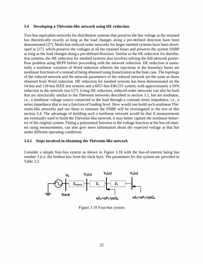
3.4.1 Steps involved in obtaining the Thévenin-like network

Consider a simple four-bus system as shown in Figure 3.18 with the bus-of-interest being bus

number 3 (i.e. the farthest bus from the slack bus). The parameters for this system are provided in

Table 3.2.

V0

Slack

Z1

AC

αS2=αP2+jαQ2

Z2

αS3=αP3+jαQ3

V2(α) V3(α)

Zsource

V1(α)

Figure 3.18 Four-bus system

23

Table 3.2 System parameters for four-bus system

Parameter name Value Parameter name Value

S2 50.0 + 10.0j (MVA) ZSource 0.01j (Ω-pu)

S3 10.0 + 5.0j (MVA) V0 1.0 pu

Z1 0.01 + 0.1j (Ω-pu) MVABase 100 MVA

Z2 0.02 + 0.2j (Ω-pu)

The first step to obtain the Thévenin-like network is to reduce the original system to a three-bus

network as shown in Figure 3.19, obtained by eliminating bus number 2 using HE reduction. The

current injection at bus number 2, I2(α) is given by:

**

2

*

22

V

SI

(3.16)

The functions I1_2(α) and I3_2(α) represent the parts of the external (nonlinear) current injections

(i.e., I2(α)), that are moved to the boundary buses, i.e., bus 1 and bus 3, respectively, for this sys-

tem. The reason bus 1 is retained in the reduced network (and this is important) is to avoid a part

of the external current injection being moved to the slack bus, since the system effects of such a

current source (in parallel with a voltage source at the slack bus) are lost and the model, therefore,

becomes incorrect. Note that at this stage, the slack bus power in the reduced network is the same

as that in the original full network.

V0

Slack

ZWard

AC

αS3=αP3+jαQ3

V3(α)

Zsource

V1(α)

I1_2(α) I3_2(α)

Figure 3.19 HE-reduced network

Once a network with a structure as shown in Figure 3.19 is obtained (and this topology is what we

will obtain even for more complex network reductions), we need to transform it into a Thévenin-

like network. The first step in doing this is to convert the voltage source at the slack bus to a Norton

source as shown in Figure 3.20.

24

αS3=αP3+jαQ3

V3(α)V1(α)

I1_2(α) I3_2(α)V0/Zsource

Zsource ZWard

Figure 3.20 Step1 of getting a Thévenin-like network from the HE-reduced network

Though Thévenin-Norton conversions have been shown to be strictly valid for only linear systems,

one can show that the conversion shown in Figure 3.20, preserves the load voltage and current

profiles. The net current flowing into bus 1 in the reduced network shown in Figure 3.19 should

be zero and is given by Iin_1:

W ardSource

inZ

VVI

Z

VVI

13

2_1

10

1_

(3.17)

The current flowing into bus 1 in the network shown in Figure 3.20 is:

W ardSourceSource

stepinZ

VVI

Z

V

Z

VI

13

2_1

011_1_

(3.18)

Note that the current injection into bus 1 is the same in both networks as seen from (3.17) and

(3.18). Clearly the net injection into bus 3 is also the same in both networks. Hence the load voltage

and load current are preserved in this Thévenin-Norton conversion. Given that the roots of the

voltage Padé approximants provide a tight upper bound on the SNBP, and that the voltage series

in the two networks is the same, it follows that the SNBP of the network is preserved after such a

Thévenin-Norton conversion. The net current injection at bus 1 in Figure 3.20 can then be con-

verted to a voltage source using a Norton-to-Thévenin conversion, as shown in Figure 3.21.

V0+I1_2(α)ZsourceAC

αS3=αP3+jαQ3

V3(α)

I3_2(α)

Zsource ZWard

V1(α)

Figure 3.21 Step-2 of getting a Thévenin-like network from the HE-reduced network

It can be shown that this Norton-Thévenin conversion preserves the load voltage and current de-

spite the nonlinear nature of the source. The current flowing into bus 1 in Figure 3.21 is given by:

25

W ardSource

Source

stepinZ

VV

Z

VZIVI

1312_10

2_1_

(3.19)

Note that the current injection into bus 1 is the same in the networks shown in Figure 3.20 and

Figure 3.21 as seen from (3.18) and (3.19). Hence the load voltage, load current as well as the

system SNBP are preserved through the Norton-Thévenin conversion. The voltage source can then

be converted again to a current source (again while preserving the load characteristics and the

system SNBP as shown earlier) as shown in Figure 3.22.

(Zsource +ZWard)

αS3=αP3+jαQ3

V3(α)

I3_2(α)(V0+I1_2(α)Zsource)/(Zsource +ZWard)

Figure 3.22 Step-3 of getting a Thévenin-like network from the HE-reduced network

The net current injection at bus 3 can then be converted back to a voltage source, as shown in

Figure 3.23, which is the Thévenin-like network consisting of a variable voltage source Vsource(α),

connected to the bus-of-interest through a constant impedance.

V0+I1_2(α)Zsource +I3_2(α)(Zsource +ZWard)AC

αS3=αP3+jαQ3

V3(α)

(Zsource +ZWard)

Figure 3.23 Final step of getting a Thévenin-like network from the HE-reduced network

Note that when such Thévenin-Norton conversions are performed, the slack bus power is no longer

preserved, i.e., it does not match the slack bus power from the full network. Additionally, similar

to the measurement-based Thévenin equivalent, the source voltage, Vsource(α), is not the open-cir-

cuit voltage at the bus-of-interest (if the uniform scaling HEPF formulation is used). If evaluated

at α=0, it represents the voltage the bus-of-interest when all the buses in the network are open-

circuited. One can use the direction-of-change scaling formulation to scale the load only at the

bus-of-interest, in which case Vsource(α) evaluated at α=0, represents the open-circuit voltage at the

bus-of-interest. The formulation that one uses to solve the power-flow problem for the whole net-

work depends on the study one wants to perform with the reduced model. Hence depending on the

assumptions one makes about the full-model load behavior, one should choose an appropriate scal-

ing formulation. The series impedance of the nonlinear Thévenin-like network is not the same as

26

VOC/ISC either, it is simply the series combination of Zsource and the impedance obtained from Ward

reduction i.e. ZWard. Since the loads are modeled as nonlinear current injections, it is not surprising

that the series impedance is a constant that is independent of the system loading condition. Instead,

it is Vsource that is a function of α since it is dependent on the external current injections.

While a simple radial 4-bus system was used to explain the approach for arriving at the Thévenin-

like network, no inherent assumptions are made that would restrict this approach to radial systems.

Results will be demonstrated on the meshed 14-bus system in the following sections.

Numerically validating the foregoing approach is an important component of the research ap-

proach. In order to validate the foregoing Thévenin-like network with a nonlinear voltage source,

obtained using HE reduction, the power-flow problem is solved for this reduced network to obtain

the voltage at the retained bus. The voltage solution obtained from the reduced network is com-

pared with the full network solution for the four-bus system at different load-scaling factors up to

the SNBP (estimated at load-scaling factor = 5.0243, using CPF). It was seen that the voltage

solution from the Thévenin-like network matched that obtained from the full network at all loading

levels as shown in Figure 3.24 and Figure 3.25 in which the voltage magnitudes and voltage angles

for the full and reduced networks are plotted against the load-scaling factor. The magnitude of the

difference between the voltage at the retained bus obtained from the full network and that obtained

from the Thévenin-like network is plotted against the load-scaling factor in Figure 3.26. It is seen

that the difference is on the order of 10-15 pu at load levels that are not too close to the SNBP.

Figure 3.24 Voltage magnitude from Thévenin-like network and full network, 4-bus system

27

Figure 3.25 Voltage angle from Thévenin-like network and full network, 4-bus system


and the full network, 4-bus system

For a second test case, the IEEE 14 bus system was used. Similarly, the voltage solution from the

Thévenin-like network matched that obtained from the full network for the 14-bus system at all

loading levels through to the SNBP (estimated to be at load-scaling factor = 4.012, using CPF) as

28

shown in Figure 3.27 and Figure 3.28 in which the voltage magnitudes and voltage angles are

plotted respectively for the full and reduced networks against the load-scaling factor, with the bus-

of-interest being bus number 4. Note that an additional bus, ‘bus 0’ was added to the system and

made the slack bus in the new system, connected to the original slack bus (bus number 1) in the

IEEE 14-bus system via the series impedance Zsource (assumed to be 0.01j), thus making the total

number of buses 15. This system will be referred to as the modified 14-bus system in the rest of

the document. The magnitude of difference between the voltage at the retained bus (bus number

4) obtained from the full network and that obtained from the Thévenin-like network for the modi-

fied 14-bus system is plotted against the load-scaling factor in Figure 3.29 and it is seen that the

differences are very low. The gaps in the plot represent loading levels where the error was exactly

zero, when using Matlab’s double precision arithmetic.

Figure 3.27 Voltage magnitude from Thévenin-like network and full network, modified 14-bus

system

29

Figure 3.28 Voltage angle from Thévenin-like network and full network, modified 14-bus system


and the full network, modified 14-bus system

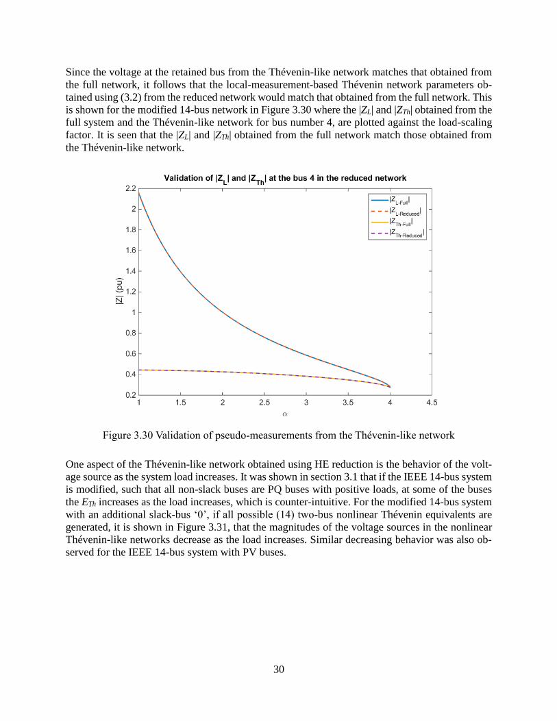
30

Since the voltage at the retained bus from the Thévenin-like network matches that obtained from

the full network, it follows that the local-measurement-based Thévenin network parameters ob-

tained using (3.2) from the reduced network would match that obtained from the full network. This

is shown for the modified 14-bus network in Figure 3.30 where the |ZL| and |ZTh| obtained from the

full system and the Thévenin-like network for bus number 4, are plotted against the load-scaling

factor. It is seen that the |ZL| and |ZTh| obtained from the full network match those obtained from

the Thévenin-like network.

Figure 3.30 Validation of pseudo-measurements from the Thévenin-like network

One aspect of the Thévenin-like network obtained using HE reduction is the behavior of the volt-

age source as the system load increases. It was shown in section 3.1 that if the IEEE 14-bus system

is modified, such that all non-slack buses are PQ buses with positive loads, at some of the buses

the ETh increases as the load increases, which is counter-intuitive. For the modified 14-bus system

with an additional slack-bus ‘0’, if all possible (14) two-bus nonlinear Thévenin equivalents are

generated, it is shown in Figure 3.31, that the magnitudes of the voltage sources in the nonlinear

Thévenin-like networks decrease as the load increases. Similar decreasing behavior was also ob-

served for the IEEE 14-bus system with PV buses.

31

Figure 3.31 Magnitude of Vsource(α) vs. α

3.4.2 Impact of modeling loads as nonlinear currents or nonlinear impedances

In the numerical results demonstrated in section 3.4.1, the loads were modeled as nonlinear current

injections. However, it is possible to model the loads as nonlinear impedances as well. This can be

shown by replacing I3_2(α) (the external current injection at bus 3) in Figure 3.21 by an equivalent

nonlinear impedance given by (3.20) as shown in Figure 3.32.

2_3

3

2_3I

VZ

(3.20)

32

(Zsource +ZWard)

αS3=αP3+jαQ3

V3(α)

(V0+I1_2(α)Zsource)/(Zsource +ZWard)Z3_2(α)


The effective series impedance in the resultant Thévenin-like network is then a parallel combina-

tion of Z3_2(α) with (Zsource+ZWard). The Thévenin-like network will appear as shown below.

{(V0+I3_2(α)Zsource)/(Zsource +ZWard)}*

{Z3_2(α)||(Zsource +ZWard)}AC

αS3=αP3+jαQ3

V3(α)

{Z3_2(α)||(Zsource

+ZWard)}


Note that in the above network, the voltage source as well as the series impedance as nonlinear

functions of α. The current flowing into bus 3 in the above network is given by:

**

3

*

3

2_3

2_3

3

2_3

2_32_10

_3_

*

V

S

ZZZ

ZZZ

VZZZ

ZZZ

ZZ

ZIV

I

W ardSource

W ardSource

W ardSource

W ardSource

W ardSource

Source

nonlinearZin

(3.21)

By substituting the expression for Z3_2(α) from (3.20) into (3.21), one gets

33

**

3

*

3

2_3

3

2_3

3

32_10

_3_

V

S

I

VZZ

I

VZZ

V

ZZ

ZIV

I

W ardSource

W ardSource

W ardSource

Source

nonlinearZin

(3.22)

By further simplification of (3.22) as given below, one can show that the net current flowing into

bus 3 in the network given by Figure 3.33 is the same as that in the network given by Figure 3.23.

**

3

*

32_3

32_10

**

3

*

332_32_10

**

3

*

3

32_3

3

32_10

_3_

V

SI

ZZ

VZIV

V

S

ZZ

VIZZ

ZZ

ZIV

V

S

VIZZ

VZZ

V

ZZ

ZIV

I

W ardSource

Source

W ardSource

W ardSource

W ardSource

Source

W ardSource

W ardSourceW ardSource

Source

nonlinearZin

(3.23)

This was tested numerically on the modified 14-bus system by solving the power-flow problem

for the network given by Figure 3.32 with a nonlinear impedance at the retained bus and it was

observed that the voltage series at the bus-of-interest matched the voltage series of that bus from

the full-network solution, with an accuracy of the order of 10-14 and the system SNBP was pre-

served as well. This shows that it is not necessary to model the loads as nonlinear current injections

that are functions of α but the loads can also be modeled as nonlinear shunt impedances. Given

that both the models can be used, there is no obvious motivation to model the loads as impedances

because that would make the admittance matrix a function of α, thus making the network reduction

very complicated and computationally expensive. Additionally, since the source voltage as well as

impedance are nonlinear in this case, if the Maclaurin series are to be estimated using local voltage

and current measurements, one would need to fit two 40th degree polynomials (the degree of the

polynomials would depend on the number of terms needed to accurately estimate the SNBP and

40 is an empirically obtained approximate number) instead of one polynomial. This would make

the process more complicated and prone to inaccuracies, particularly in the presence of noisy meas-

urements. Hence, while there is no compulsion to do so, it is recommended that the loads be mod-

eled as nonlinear current injections for ease of computation.

3.4.3 Arbitrary Thévenin-like networks

As demonstrated in section 3.4.1, depending on how the loads are modeled (nonlinear current

injections or nonlinear shunt impedances), one can get different Thévenin-like networks, while

still preserving the voltage at the load bus and the system SNBP. In fact, one can even model some

of the loads as nonlinear shunt impedances and the rest as nonlinear currents. This flexibility can

34

be extended to fixed shunt impedances as well. The traditional way of modeling fixed shunts is to

keep them as constants in the admittance matrix while performing the reduction, which would

result in fixed shunt impedances appearing in the reduced network. The other way of modeling

fixed shunt impedances is to model them as nonlinear current injections given by -YshuntV(α) before

performing the reduction (keeping in mind that all the voltage series from the full network are

available before performing the reduction). This would result in a reduced-order network that

doesn’t have any shunt impedances. Thus there are an infinite number of ways in which some/all

the shunt impedances (or even parts of the series impedances if one so desires) can be modeled as

nonlinear current injections by suitably multiplying them by the voltage series before performing

the HE-reduction. This implies that there are an infinite number of different Thévenin-like net-

works that can be obtained for any given system. The implication that this has on using measure-

ments to build the Thévenin-like networks is that, one can arbitrarily choose a value for the series

impedance and fit the series for the source voltage such that the load behavior at the bus-of-interest

is preserved. In order to prove that this can be done, consider a three-bus network obtained using

HE-reduction as shown in Figure 3.19, where only the series impedances were retained in the

admittance matrix and the shunt impedances were modeled as nonlinear current sources to yield

the model of Figure 3.19. The Thévenin-like network would consequently not have any shunt im-

pedances and would appear as shown in Figure 3.23. One can add a shunt impedance at bus 1 to

the network shown in Figure 3.23 along with a compensatory current injection as shown in Figure

3.34.

V0

Slack

ZWard

AC

αS3=αP3+jαQ3

V3(α)

Zsource

V1(α)

I1_2(α)+YaddV1(α) I3_2(α)Yadd

Figure 3.34 Shunt impedance and compensatory shunt current added at bus 1.

Note that since the additional shunt impedance is negated by an equivalent injected current, the

bus voltages and current flows in the network are still preserved. The effective input impedance of

the above network is then given by:

35

W ard

sourceadd

source

W ard

add

source

W ardaddsourceseries

ZZY

Z

Z

YZ

ZYZZ

1

1

1

/1||ˆ

(3.24)

Since the additional shunt impedance can be arbitrarily chosen, this implies that the effective

source impedance Ẑseries can also be arbitrary and the nonlinear source voltage will then ensure that

the load voltage and current characteristics are preserved. One can reverse engineer the above

process to calculate the additional shunt impedance one needs to add on to bus 1, Zadd =Yadd-1 given

by (3.25), in order to get the desired value of effective source impedance, Zdesired.

desiredW ardsource

W arddesiredsource

addZZZ

ZZZZ

(3.25)

This was verified numerically on the four-bus and 14-bus systems where the source impedance

was arbitrarily forced to be 0.01+0.1j and the necessary shunt impedance calculated from (3.27)

and compensatory current was added at bus 1. The voltage series of the bus-of-interest obtained

by solving the power-flow problem for this reduced-order network was the same as that from the

full-network with an accuracy on the order of 10-14. Thus, one can arbitrarily choose a value for

the series impedance and fit the series for the source voltage using measurements such that the

voltage at the bus-of-interest is preserved and such a model will preserve the system SNBP. Ex-

pectedly, if one chooses the series impedance value to be the measurement-based ZTh from section

3.1, that value of VS(α), evaluated at that particular loading-level, matches the measurement-based

ETh with an accuracy of 10-15. This shows that the measurement-based Thévenin equivalent net-

work, is obtained by linearizing one of the infinitely-many nonlinear Thévenin-like networks about

the base-case operating point.

3.4.4 Maximum power-transfer condition in the presence of a variable voltage source

It is known that if the voltage source and impedance are constant, the maximum power transfer to

the load occurs when the magnitude of the load impedance is equal to the magnitude of the source

impedance, i.e., |ZSource|=|ZL|. However, the Thévenin-like network developed in section 3.4 has a

voltage source that is a function of the load-scaling factor α. Hence the assumption of a constant

source is no longer valid, consequently the condition |ZSource|=|ZL| is no longer true at the maximum

power transfer point. This is shown in Figure 3.35, in which the magnitude of the load impedance

and the magnitude of the source impedance is plotted against the load-scaling factor, α. It is seen

that there is a significant difference between the magnitude of the source impedance and the load

impedance even at the SNBP which occurs at α = 4.012 obtained using CPF. Note that the source

impedance remains constant as the system load increases, which is expected.

36

Figure 3.35 |ZL(α)| and |ZSource| vs. α for the modified 14-bus system

Since the end goal is to use nonlinear HE-reduced networks to estimate the voltage stability mar-

gin, it is important to derive the condition at which maximum power transfer will occur. While

one can use the roots (poles/zeros) of the voltage series, it is not clear as to which method would

work the best when building the networks using actual noisy measurements. Hence it is important

to have alternatives such as the maximum power transfer theorem for nonlinear networks. Using

the same approach as that used for linear networks, i.e., equating to zero the derivative of the real-

power transferred to the load w.r.t. to the load resistance, the appropriate condition can be derived

as described below.

The power delivered to the load in the Thévenin-like network shown in Figure 3.23, is given by

(3.26) which is similar to (3.9), with the only difference being that ETh is replaced by VS(α) which

is the nonlinear voltage source in the Thévenin-like network and RTh ,XTh are replaced by RS, XS

which are the resistive and reactive components of the net series impedance.

22

2

)()(

)()(

LSLS

LS

L

XXRR

RVP

(3.26)

Assuming that the power factor angle of the load, Φ, is kept fixed, the load impedance can be

written as:

tan)()()()()( LLLLL jRRjXRZ (3.27)

Equation (3.26) can thus be written as:

37

22

2

)tan()()(

)()(

LSLS

LS

L

RXRR

RVP

(3.28)

The derivative of PL with respect to RL is given by:

222

2

222

222

2

)tan()()(

)tan()tan()(2)(2)()(

)tan()()(

)tan()()()()()(

)(

)(

LSLS

LSLSLS

LSLS

LSLSSL

L

S

L

L

RXRR

RXRRRV

RXRR

RXRRVRR

V

R

P

(3.29)

When the power delivered to the load is maximum, the derivative of PL with respect to RL is zero.

Equating (3.29) to zero, we get:

)tan()tan()(2)(2)()(

)tan()()()()()(

)(

2

222

2

LSLSLS

LSLSSL

L

S

RXRRRV

RXRRVRR

V

(3.30)

Equation (3.30) can be rearranged as follows:

222

2

22

)tan()()()(

)tan()tan()(2)(2)()(

)()()(

)(

LSLSS

LSLSLS

LSL

L

S

RXRRV

RXRRRV

ZZRR

V

(3.31)

The terms of the right-hand side expression can be expanded to obtain:

)tan()(2)(tan)(

)(2)(

)(tan)(2)tan()(2)(2)(2

)(

)()()(

)(

22

222

222

2

22

LSL

SLSLS

LLSLLS

S

LSL

L

S

RXR

XRRRR

RRXRRR

V

ZZRR

V

(3.32)

Equation (3.32) is reduced to:

38

222222

22

)(tan)()()(

)()()(

)(

SSLLS

LSL

L

S

XRRRV

ZZRR

V

(3.33)

Equation (3.33) can then be reduced to obtain the final maximum power transfer condition given

by (3.34) or, the theoretical equivalent in (3.35), when the source voltage is not constant.

222

22

)()(

)()()(

)(

SLS

LSL

L

S

ZZV

ZZRR

V

(3.34)

2 22

2 2

( )( ) ( )

( ) ( ) ( )

L SS L

L S S L

Z ZV R

R V Z Z

(3.35)

The Maclaurin series for the expression ∂|VS(α)|2 /∂RL(α) used in (3.34) is obtained as:

)(

)(

)(

)(

2

2

L

S

L

S

R

V

R

V

(3.36)

The Maclaurin series for |VS(α)|2 can be obtained as:

)()()( **2 SSS VVV

(3.37)

and then the derivative of |VS(α)|2 with respect to α can be calculated. For load buses with PQ loads,

the load impedance ZL(α) is given by:

*

** )()()(

S

VVZ L

(3.38)

Note that if the expression for ZL(α) on the RHS of (3.38) is expanded as a power series, one will

get a term with a negative exponent of α. Hence the expression for RL(α) will also have a term with

a negative exponent of α. In order to avoid the negative exponent, the values of the load resistance

at different values of α can be obtained using the value of αRL(α), for which the Maclaurin series

is given by (3.39),

39

*

** )()(Re)(

S

VVRL

(3.39)

where the function Re(.) indicates the real part of the operand. The value of ∂RL(α)/∂α at different

values of α can be obtained using the value of ∂αRL(α)/∂α as shown below:

)()(

)(

)()()(

LL

L

LLL

RR

R

RRR

(3.40)

It is seen that the left-hand-side (LHS) and right-hand-side expressions (RHS) of (3.34) are purely

real. However, the ∂|VS(α)|2 /∂RL(α) term on the LHS is obtained by first performing convolutions

of complex-valued power series and then taking derivatives with respect to α. While theoretically

the series should be purely real, performing a convolution of two complex-valued power series,

leads to small imaginary parts in the resultant series with magnitudes less than 10-19. At loading

levels that are not very close to the SNBP, the imaginary part of the LHS of (3.34) is observed to

be of the order of 10-15. However when the system load is modeled to be within 1% of the SNBP,

the numerically small imaginary parts in the different series involved in the LHS of (3.34) become

significant since they are multiplied by high-order exponents of α, which causes the imaginary part

of the Padé approximants of the series on the LHS to be of the order of 10-3. This is shown in

Figure 3.36 and Figure 3.37 in which the imaginary parts of the LHS and RHS of (3.34) are plotted

against α for the four-bus system and the modified 14-bus system (when bus 9 is retained), respec-

tively. Since the imaginary parts of the LHS and RHS should theoretically be zero and are numer-

ically of the order of 10-15 unless the system load is modeled to be within 1-2% of the SNBP, the

imaginary parts will be ignored in the rest of the discussion.

40

Figure 3.36 Imaginary parts of the LHS and RHS of (3.34) vs. α for the four-bus system

Figure 3.37 Imaginary parts of the LHS and RHS of (3.34) vs. α for the modified 14-bus system

The validity of the condition given by (3.34) is verified using the four-bus system shown in Figure

3.18 and the modified 14-bus system. In Figure 3.38 the LHS and RHS for the four-bus system are

41

plotted against the load-scaling factor varying up to the SNBP and it is seen that at the SNBP, the

LHS and RHS are very close to each other. Similarly, the LHS and RHS are plotted in Figure 3.39

against α for the modified 14-bus system (with the bus-of-interest chosen to be bus number 4) and

the two approach each other at the SNBP as expected. It is observed that when the system load is

modeled to be within 0.1% of the SNBP, a cross-over occurs between the values of the LHS and

RHS expressions, which can be attributed to precision issues and is left as future work. It is well-

known that precision limitations become an issue for the HEPF-based methods when the system

is modeled to be very close to the SNBP.

Figure 3.38 LHS vs. RHS of (3.34) for the four-bus system

Figure 3.39 LHS vs. RHS of (3.34) for the modified 14-bus system

42

The condition also holds true for a Thévenin-like network with an arbitrarily chosen impedance as

explained in section 3.4.3. This was verified numerically on the modified 14-bus system with the

source impedance forced to be 0.15j (while the series impedance obtained using traditional HE

reduction was approximately 0.03 + 0.1j). The necessary additional shunt impedance was calcu-

lated using (3.27) with compensatory current added at bus number 1. This is shown in Figure 3.40

where the LHS and RHS are plotted against α (varying up to the SNBP) for the above described

arbitrarily chosen Thévenin-like network, with the bus-of-interest being bus number 4.

Figure 3.40 LHS vs. RHS of (3.34) for the modified 14-bus system with an arbitrary Thévenin-

like network

3.4.5 Some implementation details

3.4.5.1 Handling ZIP-load models and arbitrary load models

While so far in this section only constant PQ loads were considered, the actual load may have ZIP-

load characteristics or other more complex characteristics which need to be accounted for appro-

priately. The model for solving a power-flow problem in the presence of ZIP-loads requires rep-

resenting all loads nonlinear current injections of α. The development is straight forward and will

not be included here. Thus the reduction process to obtain the Thévenin-like networks would be

the same as described in section 3.4.1. The maximum power transfer condition for nonlinear net-

works given by (3.34) holds true in the presence of ZIP-load models as well. While evaluating the

43

two sides of the condition, one would need to calculate the effective load impedance ZL(α) given

by:

miqVqVqQjpVpVpP

VV

Z

iiliiili

ii

L

,

32

2

132

2

1

**

(3.41)

The LHS and RHS of (3.34) are plotted against α in Figure 3.41, for the 14-bus system with ZIP

loads (equal proportions of the constant impedance, constant current and constant power assumed),

with the bus-of-interest being bus number 2. The load-scaling factor is varied through to the SNBP

in Figure 3.41 and it is seen that the LHS and RHS are numerically close to each other at the SNBP.

Figure 3.41 LHS and RHS of (3.34) for the modified 14-bus system with ZIP loads

In fact, any arbitrary load can effectively be represented as a nonlinear current injection in order

to get the Thévenin-like networks. This can be demonstrated using an arbitrary load model that

looks like:

miK

qVqVqQjpVpVpPS

i

iiliiiliL

!11!9!7!5!3

119753

32

2

132

2

1

(3.42)

The above load model looks like a ZIP-load model along with a sine-of--series accurate to 11

Maclaurin series terms. Such a load model was added at each bus in the 14-bus system with the

coefficient Ki being randomly chosen from uniformly distributed numbers between 0 and 10 MW

44

(the base-case real-power loads at the different buses vary between 3.5 MW and 94.2 MW for this

system). With this load modeled as a nonlinear current injection, the HEPF was used to solve the

power-flow problem and then HE-reduction was performed. It was observed that as long as the

reduction rules provided in this work are followed, the series terms of the voltage series (truncated

at 61 terms) at the retained bus were preserved, when compared to the full network voltage series

terms, with an accuracy of the order of 10-14 and the SNBP of the system was also preserved.

3.4.5.2 Handling transformers

3.4.5.2.1 Handling transformers with off-nominal tap ratios

Transformers with off-nominal tap ratios, are effectively modeled using pi models and hence shunt

impedances are added at the terminal buses. As explained in section 3.4.3, fixed shunt impedances

can either be represented in the admittance matrix, which would result in shunt impedances ap-

pearing in the HE-reduced network; or they may be modeled as nonlinear current injections given

by -YshuntV(α) which would result in a reduced-order network that doesn’t have any shunt imped-

ances. Eventually, whether shunt impedances are retained in the HE-reduced network or converted

to nonlinear current injections, the full model will be reduced to a Thévenin-like network shown

in Figure 3.23 if the network reduction procedure given here is followed.

3.4.5.2.2 Handling transformers with non-zero phase-shifts

Transformers with non-zero phase-shifts lead to an asymmetric admittance matrix. If the phase-

shifts are represented in the admittance matrix before performing HE-reduction, the reduced order

network will have an effective phase-shifting transformer (i.e. the admittance matrix for the re-

duced network will also be asymmetric). It was shown in [31] that in order to obtain a power-flow

solution using a non-scalable formulation in the presence of phase-shifting transformers, the asym-

metric part of the admittance matrix needs to be moved to the right-hand side of the node-balance

equation as an equivalent current injection. Phase-shifting transformers have not been accounted

for in the previously published work on network reduction [27] as it is not straightforward to seg-

regate the asymmetric components from the symmetric components using only the reduced-net-

work admittance matrix for meshed reduced-order systems. Phase-shifting transformers can be

handled in a similar manner as shunts in the system, i.e., the asymmetric components of the full-

network admittance matrix that are present due to the phase-shifting transformers, can be modeled

as nonlinear current injections before performing the HE-reduction and thus removed from the

admittance matrix. This would result in a simpler reduced-order network without any phase-shift-

ing transformer, that is structurally similar to Figure 3.23. This was numerically tested on the mod-

ified 14-bus system, by adding non-zero phase shifts to the three transformers in the system (with

the phase-shifts chosen to be 7°, 9° and 25°). It was observed that the voltages were preserved as

well as the condition given by (3.34) was obeyed at the SNBP as shown in Figure 3.42 where the

LHS and RHS of (3.34) are plotted against α with the α being varied from 1.0 (i.e., the base-case

loading condition) through to the SNBP, with the bus-of-interest being bus number 4.

45

Figure 3.42 LHS and RHS of (3.34) for the modified 14-bus system with phase-shifting trans-

formers

3.4.6 Multi-bus reduced-order equivalent networks

As mentioned in section 3.1, multi-bus equivalent networks have been used to estimate the voltage

stability margin using the measurements in a load area in order to better account for the different

limits of individual tie-lines connecting the load area to the rest of the network [24], [38], [43] -

[45]. Hence it may be desirable to develop multi-bus nonlinear equivalent networks as well. It has

already been shown that HE-reduction can be used to obtain multi-bus reduced-order equivalent

networks which preserve the nonlinear behavior of the original system when there are no phase-

shifting transformers in the system [27]. Using the strategy described in section 3.4.5.2 for mod-

eling phase-shifters, multi-bus reduced networks can also developed for systems with phase-shift-

ing transformers such that the voltages at the retained buses are preserved. This is shown in Figure

3.43, in which the magnitude of worst error (taken over all retained buses) between the bus volt-

ages of the full network and those of the reduced network is plotted on a log scale against α for the

14-bus system with three phase-shifting transformers, when buses 0, 1, and 9 through 11 are pre-

served in the reduced network.

46

Figure 3.43 Error between the voltages of the full system and a multi-bus reduced-order system

for the 14-bus system with phase-shifting transformers

As pointed out in section 3.4.3, there are an infinite number of ways of developing such reduced-

order networks. Consider a reduced-order network obtained using HE-reduction with the admit-

tance matrix YReduced given by (3.43), where the subscripts b and i denote the boundary (i.e. buses

that are connected to the buses that have been eliminated), and internal buses respectively.

ii

bi

ib

bb

ducedY

Y

Y

YYRe

(3.43)

The node-balance equations in the reduced network are given by (3.44) where the subscripts e

denotes external buses (i.e., buses in the full model that are not a part of the reduced network). As

seen from (3.44) the boundary buses have additional current injections given by I’e(α) that account

for the injections and losses in the external network (i.e., in addition to the native loads at these

buses).

***

***'

ii

bbe

i

b

ii

bi

ib

bb

WS

WSI

V

V

Y

Y

Y

Y

(3.44)

Note just as there is much flexibility in selecting the value of the series impedance branch for a

two-bus equivalent, there is similar flexibility for a multi-bus equivalent. One can modify the ad-

mittance matrix (and hence the series impedances) of the reduced network by adding compensatory

nonlinear current injections on the RHS of (3.44) as shown below:

47

i

b

iiii

bibi

ibib

bbbb

ii

bbe

i

b

iiii

bibi

ibib

bbbb

i

b

ii

bi

ib

bb

V

V

YY

YY

YY

YY

WS

WSI

V

V

YY

YY

YY

YY

V

V

Y

Y

Y

Y

'

'

'

'

***

***'

'

'

'

'

(3.45)

Thus the modified admittance matrix of the reduced network is given by (3.46) and the modified

current injections are given by (3.47).

'

'

'

'

Reˆ

ii

bi

ib

bb

ducedY

Y

Y

YY

(3.46)

i

b

iiii

bibi

ibib

bbbb

ii

bbe

ducedV

V

YY

YY

YY

YY

WS

WSII

'

'

'

'

***

***'

Reˆ

(3.47)

In fact, not only can the impedance values in the HE-reduced network be modified using (3.45),

but the topology can also be changed, though we believe in most cases it is unwise to do so. One

could add additional branches that did not exist in the HE-reduced network. For example, for the

14-bus system with three phase-shifting transformers, when buses 0, 1, 9 through 11 are preserved

in the reduced network, there is no connection between bus number 1 and bus number 10. How-

ever, a branch with impedance 0.01+0.1j was added between these two buses and compensatory

currents added at buses 1 and 10 using (3.45). When the power-flow problem for such a reduced

network was solved, it was observed that each term of the truncated Maclaurin voltage series (up

to 61 terms) at all the retained buses in the new reduced network, matched those from the full

network, with an accuracy of the order of 10-14. Similarly, one could remove an existing branch by

setting Y’ik to be zero. For the 14-bus system reduction example described above, two branches

were removed to effectively obtain a radial reduced-order network, while still preserving each term

of the truncated voltage series (up to 61 terms) at the retained buses with an accuracy of the order

of 10-14 when compared to the voltage series for the full model.

The implication that this has on using measurements to build multi-bus equivalent networks is that,

one does not need to know the appropriate topology and network parameters prior to building the

network, though it is believed results would be best if the topology chosen matches that in the real

world. One can assume a certain topology and network parameters for the reduced network and fit

the Maclaurin series for the nonlinear current injections using measurements at the retained buses.

Note that the multi-bus reduced order networks, require more polynomials to be fitted than the

Thévenin-like equivalent networks since each bus has a nonlinear current injection.

3.5 Revisiting the sigma method

It was shown in [51] that the original sigma method as shown in [33], has some fundamental flaws.

It was shown that while it is true that to ensure a valid operating point for any system, the sigma

48

condition must be obeyed for all of the system buses, the proximity of the σ condition to violating

its limit at any of the buses is not an indicator of the proximity of the system to voltage collapse.

This occurs because the σ indices of some of the buses can come very close to the boundary con-

dition at loading levels far below the SNBP, and then start moving away from the boundary with

further load increase. The fundamental issue is that, while the distance of the σ condition from its

limit is an indicator of the proximity of the system to voltage collapse for a two-bus system, it is

not an indicator for a two-bus equivalent of a larger system. The voltage source in the two-bus

equivalent from which the original σ indices are obtained is constant (slack-bus voltage) whereas

it has been shown in section 3.4 that a proper equivalent obtained using network-reduction proce-

dures where the loads are modeled as nonlinear current injections would have a voltage source that

depends on the loading condition. It will be shown numerically that if the σ indices are calculated

corresponding to the Thévenin-like network obtained in section 3.4, these revised σ indices do not

face the same issues as the original σ indices. The U(α) for the Thévenin-like network as shown in

[51] is given by:

)(

)()(

sourceV

VU

(3.48)

Substituting the above expression for U(α) into the performance equation for the two bus equiva-

lent as shown in [51], one gets the revised σ indices, with the only difference being that U(α) is no

longer V(α)/VSlack but is given by (3.48). For the four-bus system from Figure 3.18, the σ condition

at buses 3 and 4, evaluated using the original and revised σ indices are plotted against the load-

scaling factor α in Figure 3.44. It is seen that the use of the original σ indices causes the σ condition

at bus 4 be very close to zero at α = 4.85 and then bounce back, whereas the σ condition at both

buses evaluated using the revised σ indices have a consistent decreasing behavior as α increases.

The other claim made in [33] was that the buses that are closer to violating the σ condition can be

deemed to be the “weak buses” in the system. As discussed in [51], theoretically there is no clear

connection between the sigma method of determining weak buses and the modal analysis method

of determining weak buses. Using modal analysis [35], the weak bus for this small system is con-

sistently obtained to be bus number 4 at different loading conditions (nearly 20%, 40%, 60%, 80%

and 100% of the SNBP loading). However, it is seen that the “weak” bus obtained using the revised

σ condition is not consistent at all loading conditions, shown by the cross-over in Figure 3.44. It is

seen from Figure 3.44 that even when using the revised σ indices, at most operating conditions the

“weak” bus obtained using the σ condition does not match that obtained using modal analysis,

despite the small size and radial nature of the system being tested.

49

Figure 3.44 Original and revised σ conditions vs. α for the four-bus system

The σ scatter plot for bus number 4 as the system load increases is shown in Figure 3.45. The “turn-

around” of the original σ index in Figure 3.45 occurs at α = 4.85, which is consistent with its “turn-

around” point observed on the σ condition plot in Figure 3.44.

Figure 3.45 σ scatter plot with original and revised σ indices, bus 4

50

The σ condition with the revised σ indices was observed to have consistent behavior with load

increase for the modified 14-bus system as well, as opposed to the σ condition with the original σ

indices. This is shown in Figure 3.46 and Figure 3.47 where the value of the σ condition for the

PQ buses is plotted against α for the revised and original σ indices respectively. Note that bus 7

has no load on it and hence the Vsource(α) is the same as V(α) which causes the U(α) to be a constant

(1.0) and hence the σ condition for bus 7 using the revised σ index remains constant as seen from

Figure 3.46.

Figure 3.46 σ condition vs. α with revised σ indices, modified 14-bus system

Figure 3.47 σ condition vs. α with original σ indices, modified 14-bus system

While the revised σ indices resolve the issue of approaching the boundary condition well ahead of

the SNBP and then increasing again, it is seen from Figure 3.46 that for some of the buses, the σ

51

condition has a somewhat flat profile as the system load increased and then a sharp decrease as the

modeled load gets very close to the SNBP. This highly nonlinear behavior of the σ condition,

makes it unfavorable to use the σ condition as a measure of the proximity to the SNBP, even with

the revised σ indices. Additionally, even for the revised σ indices, no correlation was found be-

tween the “weak buses” obtained using the σ condition and the “weak buses” from modal analysis,

for the modified 14-bus system.

3.6 Conclusions

In this chapter, the measurement-based method of building a Thévenin equivalent at the bus-of-

interest is discussed along with the impact that discrete changes can have on such purely local-

measurement-based methods of estimating the SNBP. HE-reduction was used to build nonlinear

Thévenin-like networks which preserved the nonlinearity of the original system. Using measure-

ments, the polynomials in such a nonlinear Thévenin-like network can be fitted and it was shown

that one can assume any value for the source impedance and the source voltage Maclaurin series

can then be appropriately calculated. The maximum power transfer theorem for such nonlinear

networks was derived and validated, while accounting for ZIP-load models and phase-shifting

transformers. While multi-bus nonlinear reduced-order networks can also be built, these would

require a greater number of polynomials to be fitted and hence are more complicated, particularly

in the presence of noisy measurements. While the original sigma indices were modified such that

their behavior became monotonic as the system load increased, it was observed that the revised

sigma indices could still not easily be used to determine the weak buses in the system. In this work,

it was assumed that the load changes along a pre-defined direction, and hence when measurements

are used to build a nonlinear Thévenin-like network, the network will be fitted for a particular

pattern of load/generation change. Once the nonlinear Thévenin-like network is built using meas-

urements, if the loading vector changes drastically, the estimated SNBP may not be accurate. This

will have to be carefully investigated going forward.

52

4. Fitting Methods in Detail and the Roots Methods

4.1 Different numerical methods for estimating the SNBP from measurements

In section 3.4.4, the maximum power transfer theorem (MPTT) was developed to estimate the

SNBP for the nonlinear reduced network. Therefore, in this section, numerical experiments using

noiseless pseudo-measurements to estimate the SNBP from the MPTT given by (3.35) will be

conducted. The effects of noise in the measurements will be discussed in later sections.

4.1.1 Fit a function of α from noiseless measurements

Since the main process in these experiments is to build the functions of 𝛼 for each component in

(3.34) using noiseless data, different possible approaches to fit a general function of 𝛼 from

measurements will be first discussed in this section.

For a given function of 𝛼, 𝑓(𝛼), as shown in Figure 4.1, a number of pseudo-measurements in

the sample range ( for example, 60%-70% of the SNBP in this figure) were generated and a curve

fit to the samples in this range with the goal of projecting the value of 𝑓(𝛼) beyond the sample

range, up to the SNBP. The measurements can be used to fit either a polynomial or a Padé approx-

imant to 𝑓(𝛼). Three different approaches for fitting 𝑓(𝛼) were used: the Matlab built-in Padé

fit, self-coded Padé fit and polynomial fit are discussed in the following sections

Figure 4.1 Function of 𝛼 vs. loading-scale factor

4.1.1.1 Self-coded Padé fit

In this case, a rational function of the following form was assumed,

𝑓(𝛼) = ∑ 𝑐𝑖

𝑁

𝑖=0

𝛼𝑖 =∑ 𝑎𝑖

𝑀𝑖=0 𝛼𝑖

∑ 𝑏𝑖𝑀+1𝑖=0 𝛼𝑖

= [𝑀/𝑀 + 1]𝑓𝛼

(4.1)

53

2𝑀 + 2 = 𝑁

𝑏0 = 1

where 𝑁 is the degree of the Maclaurin series of 𝑓(𝛼), M and M+1 are the degrees of the numer-

ator and denominator polynomial of the Padé approximant, respectively. For a total of 𝑁𝑚𝑒𝑎𝑠𝑢𝑟𝑒

measurements sampled over the range of loading values selected for training, ( 𝛼𝑘, 𝑘 =1,2, … , 𝑁𝑚𝑒𝑎𝑠𝑢𝑟𝑒), the corresponding overdetermined set of equations shown in (4.2) was solved

to calculate the unknown Padé approximant coefficients 𝛼𝑖, and 𝑏𝑖. Note that the Padé approxi-

mant coefficients, 𝛼𝑖 and 𝑏𝑖, are written in ascending order of exponents of α.

∑ 𝑎𝑖

𝑀

𝑖=0

𝛼𝑘𝑖 − 𝑓(𝛼𝑘) ( ∑ 𝑏𝑖

𝑀+1

𝑖=1

𝛼𝑘𝑖 ) = 𝑓(𝛼𝑘)

(4.2)

4.1.1.2 Matlab built-in Padé fit

Similar to the above approach, a set of linear overdetermined equations was solved to directly

obtain the coefficients of the Padé approximant. The only difference is that the coefficients, 𝛼𝑖

and 𝑏𝑖 are written in descending order of exponents of 𝛼 as given by (4.3).

∑ 𝑎𝑖

0

𝑖=𝑀

𝛼𝑘𝑖 − 𝑓(𝛼𝑘) ( ∑ 𝑏𝑖

1

𝑖=𝑀+1

𝛼𝑘𝑖 ) = 𝑓(𝛼𝑘)

(4.3)

Though the self-coded Padé fit and Matlab built-in Padé fit are theoretically identical, the subtle

difference in the order of coefficients could lead to very different numerical performance. Thus,

both will be tested in a subsequent section.

4.1.1.3 Polynomial fit

In this approach, the measurements are used to fit a polynomial to 𝑓(𝛼), i.e., to obtain the 𝑐𝑖

coefficients in (4.1). The set of equations used to calculate the coefficients is indicated in (4.4):

∑ 𝑐𝑖

𝑁

𝑖=0

𝛼𝑘𝑖 = 𝑓(𝛼𝑘)

(4.4)

4.1.2 Four numerical methods for estimating the SNBP from measurements

As demonstrated in section 4.1.1, there are three approaches to fit the measurements for 𝑓(𝛼),

while fitting the measuerments for each component in (3.35) is more complicated. For example,

for |𝑉𝑠(𝛼)|2 in (3.35), one can choose to directly fit the polynomial or Padé approximant to the

Macluarin series for |𝑉𝑠(𝛼)|2 by squaring the magnitude of the source voltage measurements or

by fitting the polynomial or Padé approximant to 𝑉𝑠(𝛼) from source voltage measurements and

54

then obtain |𝑉𝑠(𝛼)|2 calculated from the polynomial or Padé approximant of 𝑉𝑠(𝛼) evaluated at

different loading-scale factors. Therefore, there are a number of combinations of the ways pseudo-

measurements can be used to fit each constituent term in (3.35) and which fitting technique

discribed in section 4.1.1 is applied.

Because the Padé approximant is sensitive to roundoff error in the calculations and because the

differences in numerical performance of different methods might become significant when

building the networks using noisy measurements, it is important to find the best method for

estimating the SNBP based on MPTT from measured data. Therefore, four possible numerical

methods are discussed in the following section. Their numerical performance was tested on the

IEEE 118 bus system. Noiseless pseudo-measuements were generated for loadings in the range of

60%-70% of the maximum system load (SNBP) using MATPOWER and a power-mismatch con-

vergence tolerance of 10-8 (For the Best Component method demonstrated in section 4.1.2.2, the

tested system is the modified 118 bus system and the sample range is 70%-80% of the SNBP). In

each case, 200 measurements were used to fit 61 terms of a polynomial or [30/30] Padé

approximant to each component in (3.35). The SNBP is estimated based on the following two

approaches: The SNBP point is taken as the eareliest point where either 1) the LHS and RHS

values of (3.35) cross each other, or 2) LHS and RHS values were initially converging and then

began to diverge.

4.1.2.1 Built-In/Self-Coded method

The MPTT equation given by (3.35) consists of six different components: 𝑍𝑠 , 𝑅𝐿(𝛼), 𝑍𝐿(𝛼),

|𝑉𝑠(𝛼)|2 , 𝜕|𝑉𝑠(𝛼)|2 𝜕𝛼⁄ and 𝜕𝑅𝐿(𝛼) 𝜕𝛼⁄ from here on abbreviated 𝜕|𝑉𝑠(𝛼)|2 and 𝜕𝑅𝐿(𝛼) ,

respectively. The variable 𝑍𝑠 is the source impedance of the Thévenin-like network obtained from

HEM/Ward network reduction and it is a constant value. Thus there is no need to calculate 𝑍𝑠

from measurements. 𝑅𝐿(𝛼) is the resistive component of the load impedance 𝑍𝐿(𝛼). Once 𝑍𝐿(𝛼)

is obtained, 𝑅𝐿(𝛼) can be calculated by taking the real part of 𝑍𝐿(𝛼). Therefore, there are only

four components that need attention: 𝑍𝐿(𝛼), |𝑉𝑠(𝛼)|2, 𝜕|𝑉𝑠(𝛼)|2 and 𝜕𝑅𝐿(𝛼).

One simple approach is to directly get 𝑍𝐿(𝛼) , |𝑉𝑠(𝛼)|2 , 𝜕|𝑉𝑠(𝛼)|2 and 𝜕𝑅𝐿(𝛼) as Padé

approximants from their respective measurements, though sometimes this has been handled

differently. For example, the function|𝑉𝑠(𝛼)|2, was built by fitting a Padé approximant to samples

of 𝑉𝑠 to yield 𝑉𝑠(𝛼)and then |𝑉𝑠(𝛼)|2 was calculated by evaluating the square of the magnitude

of 𝑉𝑠(𝛼). The implemention details are summarized in Table 4.1. Note that the measurement

𝜕|𝑉𝑠(𝛼)|2 is obtained by calculating the increment in |𝑉𝑠|2 divided by the increment in loading-

scale factor, i.e., ∆|𝑉𝑠|2/∆𝛼. The ∆𝛼 should be small enough so that the 𝜕|𝑉𝑠|2 measurement can

accurately represent the derivative of |𝑉𝑠|2 with respect to 𝛼 in the original system but at the same

time making sure there is sufficient distance between two successive points to identify the voltage

change. In this experiment, the ∆𝛼 is chosen to be 10-6. A similar approach is used to get ∂𝑅𝐿

measurements.

55

Table 4.1 Built-In/Self-Coded method

Components Pseudo-measurements Algorithm for fitting measurements

𝑍𝑠 Source impedance from HEM/Ward network reduction

𝑅𝐿(𝛼) Real part of 𝑍𝐿(𝛼)

𝑍𝐿(𝛼) 𝑍𝐿 Built-In/Self-Coded Padé-fit 𝑍𝐿

|𝑉𝑠(𝛼)|2 𝑉𝑠 1. Built-In/Self-Coded Padé-fit 𝑉𝑠

2. Get |𝑉𝑠|2

𝜕|𝑉𝑠(𝛼)|2 𝜕|𝑉𝑠|2 ( |𝑉𝑠1|2−|𝑉𝑠2|2

∆𝛼 ) Built-In/Self-Coded Padé-fit 𝜕|𝑉𝑠|2

𝜕𝑅𝐿(𝛼) 𝜕𝑅𝐿 ( |𝑅𝐿1|2−|𝑅𝐿2|2

∆𝛼 ) Built-In/Self-Coded Padé-fit 𝜕𝑅𝐿

The LHS and RHS of MPTT equation for the IEEE 118 bus system are plotted against 𝛼 in Figure

4.2 and Figure 4.3 for buses 44 and bus 67, respectively. The SNBP of the 118 bus system is 3.187,

obtained using the CPF. Bus 44 and bus 67 are selected intentionally to represent one weak bus

and one strong bus, respectively, in the 118 bus system (indentified by the magnitude of voltage

change for a given load change near the SNBP). It is seen that for the weak bus, bus 44, both the

Built-In and Self-Coded methods can give an accurate estimation of the SNBP, which are 3.179

and 3.181, respectively, with only 0.25% and 0.19% errors, respectively. However, in Figure 4.3,

neither Built-In nor the Self-Coded methods give a prediction of the SNBP for the strong bus, bus

67, regardless of whether we use the crossover or the divergence criterion. In other words, the

Built-In and Self-Coded methods work well for weak buses but do not work well for strong buses

in the system.

56


IEEE 118 bus system


IEEE 118 bus system

57

4.1.2.2 Best Component method

In this method, for each constituent of (3.35), (𝑍𝐿(𝛼), |𝑉𝑠(𝛼)|2, 𝜕|𝑉𝑠(𝛼)|2 and 𝜕𝑅𝐿(𝛼))， all of

the different ways of fitting the measurements previously mentioned are considered. Note that the

118 bus system here is modified by adding S=1+1j MVA to bus 30, bus 37 and bus 38. The loading

value at the SNBP for this modified 118 bus system is 3.172. The loading range for training data

obtained as pseudo-measurements is 70%-80% of the SNBP.

First of all, we calculate the “true” value of those variables in the 80%-100% loading range using

a 220-digit HEM implementation to obtain the accurate reference values for this range. Then the

predictions of these four components are compared with their “true” values in the 90%-100%

range. For each component, the representation that most accurately fit the true value was selected

as the best way. The best algorithm for building each component is listed in Table 4.2.

Table 4.2 Best Component method

Components Pseudo-measurements Best algorithm for fitting measurements

𝑍𝑠 Source impedance from HEM/Ward network reduction

𝑅𝐿(𝛼) Real part of 𝑍𝐿(𝛼)

𝑍𝐿(𝛼) 𝑍𝐿 Built-In Padé-fit 𝑍𝐿

|𝑉𝑠(𝛼)|2 |𝑉𝑠|2 Self-Coded Padé-fit 𝑉𝑠

𝜕|𝑉𝑠(𝛼)|2 𝜕|𝑉𝑠|2 ( |𝑉𝑠1|2−|𝑉𝑠2|2

∆𝛼 ) Self-Coded Padé-fit 𝜕|𝑉𝑠|2

𝜕𝑅𝐿(𝛼) 𝜕𝑅𝐿 ( |𝑅𝐿1|2−|𝑅𝐿2|2

∆𝛼 ) Self-Coded Padé-fit 𝜕𝑅𝐿

The LHS and RHS of the MPTT equation using the Best Component method for the modified 118

bus system with the buses-of-interest being buses 22 and 67 are plotted against 𝛼 in Figure 4.4

and Figure 4.5, respectively. The curves labeled 1) “LHS-mp220”, 2) “LHS-Built-In”, 3) “LHS-

Self-Coded” and 4) “LHS-Best-Component” represent the LHS of MPTT value of Padé

approximant 1) from network reduction using 220 digit precision, 2) from measurements using the

Built-In method, 3) from measurements using the Self-Coded method and 4) from measurements

using the Best Component method. The legend beginning with “RHS-” stands for the RHS of the

MPTT value of the Padé approximant. For bus 22, which is a weak bus in the system, the Best

Component method is shown to be better than the Buit-In and the Self-Coded methods, but not

significantly better. This slightly superior performance has also been seen for some other weak

buses when the measurement range remains to be 70%-80%. However, this method does not work

58

well for a strong bus since there is no point where the LHS and RHS cross each other or diverge

and thus no prediction can be made as shown in Figure 4.5 (the yellow and purple line).


modified 118 bus system


modified 118 bus system

59

4.1.2.3 Polynomial Method

The Polynomial Method generates polynomials (rather than Padé approximants) of all functions

of α in (3.35). To do that, each component in (3.35) needs to be reformulated to adapt to

polynomial form. The process is described below:

The load voltage 𝑉𝐿(𝛼) can be obtained as a Maclaurin series as given by (4.5) from HEM net-

work reduction.

𝑉𝐿(𝛼) = 𝑉𝐿[0] + 𝑉𝐿[1]𝛼 + ⋯ + 𝑉𝐿[𝑛]𝛼𝑛 + ⋯ (4.5)

The Maclaurin series for 𝑍𝐿(𝛼) is given by

𝑍𝐿(𝛼) =𝑉𝐿(𝛼) ∙ 𝑉𝐿

∗(𝛼)

𝛼𝑆∗

(4.6)

Note that if the expression for 𝑍𝐿(𝛼) on the RHS of (4.6) is expanded as a power series using

(4.5), one will get a term with a negative exponent of 𝛼. The expression for 𝑅𝐿(𝛼) will also have

a term with a negative exponent of 𝛼. To avoid the negative exponent, the values of the load

impedance and load resistance at different values of 𝛼 can be obtained using the value of 𝛼𝑍𝐿(𝛼)

and 𝛼𝑅𝐿(𝛼) respectively. The corresponding Maclaurin series are given below:

𝛼𝑍𝐿(𝛼) =𝑉𝐿(𝛼) ∙ 𝑉𝐿

∗(𝛼∗)

𝑆∗

(4.7)

𝛼𝑅𝐿(𝛼) = 𝑅𝑒(𝛼𝑍𝐿(𝛼)) (4.8)

The value of ∂𝑅𝐿(𝛼) at different values of 𝛼 can be obtained using the value of ∂[𝛼𝑅𝐿(𝛼)]/𝜕𝛼

as shown below:

)()(

)(

)()()(

LL

L

LLL

RR

R

RRR

(4.9)

By multiplying the top and bottom of (3.35) on both sides by 𝛼2, one can obtain:

𝜕|𝑉𝑠(𝛼)|2

|𝑉𝑠(𝛼)|2

𝛼 ∙ [𝛼𝑅𝐿(𝛼)]

𝛼 ∙ [𝛼𝜕𝑅𝐿(𝛼)]=

|𝛼𝑍𝐿(𝛼)|2 − 𝛼2|𝑍𝑠|2

|𝛼𝑍𝑠 + 𝛼𝑍𝐿(𝛼)|2

(4.10)

Substitute (4.9) into the above equation, the modified MPTT equation for Polynomial Method is

obtained, as given by (4.11).

60

𝜕|𝑉𝑠(𝛼)|2

|𝑉𝑠(𝛼)|2

𝛼 ∙ [𝛼𝑅𝐿(𝛼)]

𝛼 ∙ 𝜕[𝛼𝑅𝐿(𝛼)] − 𝛼𝑅𝐿(𝛼)=

|𝛼𝑍𝐿(𝛼)|2 − 𝛼2|𝑍𝑠|2

|𝛼𝑍𝑠 + 𝛼𝑍𝐿(𝛼)|2 (4.11)

It can be observed that the reformulated equation given by (4.11) consists of six parts:

① |𝛼𝑍𝐿(𝛼)|2 − 𝛼2|𝑍𝑠|2 , ② |𝛼𝑍𝑠 + 𝛼𝑍𝐿(𝛼)|2, ③ 𝛼 ∙ [𝛼𝑅𝐿(𝛼)] ,④ 𝛼 ∙ 𝜕[𝛼𝑅𝐿(𝛼)] − 𝛼𝑅𝐿(𝛼) ,

⑤ |𝑉𝑠(𝛼)|2 , ⑥ 𝜕|𝑉𝑠(𝛼)|2. The next step is to figure out how to get polynomials for ①-⑥ in

(4.11) from pseudo-measurements, which are shown below:

①|𝛼𝑍𝐿(𝛼)|2 − 𝛼2|𝑍𝑠|2:

The nth degree polynomial for α𝑍𝐿(𝛼) can be caluclated from 𝛼𝑍𝐿 measurements over a range of

loading values (𝛼𝑘, 𝑘 = 1,2, … 𝑁𝑚𝑒𝑎𝑠𝑢𝑟𝑒) using the polynomial fit techinique. The polynomial

expression for 𝛼𝑍𝐿(𝛼), also named as 𝑍1(𝛼), is shown in (4.12).

α𝑍𝐿(𝛼) = 𝑍1(𝛼) = 𝑍1[0] + 𝑍1[1]𝛼 + 𝑍1[2]𝛼2 + ⋯ +𝑍1[𝑛]𝛼𝑛 (4.12)

Once 𝛼𝑍𝐿(𝛼) is obtained, the |𝛼𝑍𝐿(𝛼)|2, also labeled 𝑍2(𝛼), can be calculated using (4.13):

|𝛼𝑍𝐿(𝛼)|2 = 𝑍2(𝛼) = 𝑍1(𝛼) ∙ 𝑍1∗(𝛼∗)

= 𝑍2[0] + 𝑍2[1]𝛼 + 𝑍2[2]𝛼2 + ⋯ + 𝑍2[2𝑛]𝛼2𝑛

(4.13)

Note that the |𝛼𝑍𝐿(𝛼)|2 is represented as a 2n-degree polynomial instead of being truncated to

an nth degree polynomial to avoid losing information from 𝑍1(𝛼). The varible 𝑍𝑠 represents the

source impedance obtained by network reduction and is a constant. Therefore, ① is obtained by

adding (4.13) where the 2nd order term 𝛼2|𝑍𝑠|2, is given by (4.14).

|𝛼𝑍𝐿(𝛼)|2 − 𝛼2|𝑍𝑠|2

= 𝑍2[0] + 𝑍2[1]𝛼 + (𝑍2[2] − |𝑍𝑠|2)𝛼2 + ⋯ + 𝑍2[2𝑛]𝛼2𝑛

(4.14)

② |𝛼𝑍𝑠 + 𝛼𝑍𝐿(𝛼)|2:

Similarly, the expression 𝛼𝑍𝑠 + 𝛼𝑍𝐿(𝛼) is obtained by adding (4.12) with a 1st order term 𝛼𝑍𝑠

as given by (4.15).

|𝛼𝑍𝐿(𝛼)|2 − 𝛼2|𝑍𝑠|2

= 𝑍2[0] + 𝑍2[1]𝛼 + (𝑍2[2] − |𝑍𝑠|2)𝛼2 + ⋯ + 𝑍2[2𝑛]𝛼2𝑛

(4.15)

Then ② can be calculated using the following equation:

|𝛼𝑍𝑠 + 𝛼𝑍𝐿(𝛼)|2 = 𝑍3(𝛼) = [𝛼𝑍𝑠 + 𝛼𝑍𝐿(𝛼)] ∙ [𝛼𝑍𝑠 + 𝛼𝑍𝐿(𝛼)]∗

= 𝑍3[0] + 𝑍3[1]𝛼 + ⋯ 𝑍3[2𝑛]𝛼2𝑛

(4.16)

③ 𝛼 ∙ [𝛼𝑅𝐿(𝛼)]:

61

The polynomial for α𝑅𝐿(𝛼) is calculated by taking the real part of 𝛼𝑍𝐿(𝛼), and then multiply it

with 𝛼. The process is shown below:

𝛼𝑅𝐿(𝛼) = 𝑅1(𝛼) = 𝑅𝑒(𝛼𝑍𝐿(𝛼))

= 𝑅1[0] + 𝑅1[1]𝛼 + ⋯ 𝑅1[𝑛]𝛼𝑛

(4.17)

𝛼 ∙ [𝛼𝑅𝐿(𝛼)] = 𝛼𝑅1(𝛼) = 𝑅1[0]𝛼 + 𝑅1[1]𝛼2 + ⋯ +𝑅1[𝑛]𝛼𝑛+1 (4.18)

④ 𝛼 ∙ 𝜕[𝛼𝑅𝐿(𝛼)] − 𝛼𝑅𝐿(𝛼)

The polynomial for 𝜕[𝛼𝑅𝐿(𝛼)] is obtained by taking the derivative of 𝛼𝑅𝐿(𝛼) with respect to 𝛼

as shown below:

𝜕[𝛼𝑅𝐿(𝛼)] = 𝑅2(𝛼) =𝜕𝑅1(𝛼)

𝜕𝛼 (4.19)

= 𝑅2[0] + 𝑅2[1]𝛼 + ⋯ 𝑅2[𝑛 − 1]𝛼𝑛−1

Then ④ is given by:

𝛼 ∙ 𝜕[𝛼𝑅𝐿(𝛼)] − 𝛼𝑅𝐿(𝛼) = = 𝛼 ∙ ( 𝑅2[0] + 𝑅2[1]𝛼 + ⋯ 𝑅2[𝑛 − 1]𝛼𝑛−1)

− (𝑅1[0] + 𝑅1[1]𝛼 + ⋯ 𝑅1[𝑛]𝛼𝑛)

= −𝑅1[0] + ( 𝑅2[0] − 𝑅1[1])𝛼 + ⋯ + ( 𝑅2[𝑛 − 1] − 𝑅1[𝑛])𝛼𝑛

(4.20)

⑤ |𝑉𝑠(𝛼)|2:

The nth order polynomial for 𝑉𝑠(𝛼) is obtained from the source voltage measurements using the

polynomial fit technique and then ⑤ is obtained by using (4.21).

|𝑉𝑠(𝛼)|2 = 𝑉𝑠(𝛼) ∙ 𝑉𝑠∗(𝛼∗) (4.21)

⑥ 𝜕|𝑉𝑠(𝛼)|2:

The term ⑥ is obtained by taking the derivative of the polynomial for ⑤ with respect to 𝛼.

The MPTT results using the Polynomial Method for weak bus 44 and strong bus 67 are plotted in

Figure 4.6 and Figure 4.7, respectively. The labels “LHS-MODEL-Polynomial” and “RHS-

MODEL-Polynomial” represent the LHS and RHS values, respectively, of (4.11) obtained using

network reduction techniques [27]. The labels “LHS-Polynomial” and “RHS-Polynomial”

represent the LHS and RHS values of (4.11), respectively, obtained by fitting measurements to a

polynomial. Observe that the Polynomial Method can give a reasonable estimate (by using the

divergence criterion in this case) when obtaining the power series from network reduction.

However, when using the polynomials obtained from measurements, this method does not

extrapolate the LHS well far away from the training data range. Therefore, use of the Polynomial

Method is not feasible for predicting the SNBP.

62


IEEE 118 bus system


IEEE 118 bus system

63

4.1.2.4 𝐙𝐭𝐡(𝛂) method

The idea of the 𝑍𝑡ℎ(𝛼) method is similar to conventional TE-based method. The rest of the system

is modeled as a voltage source connected through a Thévenin impedance as shown in Figure 4.8.

Note that unlike the Thévenin-like network, in which the impedance 𝑍𝑠 from HE-reduction is

constant, the Thévenin impedance in Figure 4.8 is a function of 𝛼. It can be calculated based on

its definition:

𝑍𝑡ℎ(𝛼) = −

𝜕𝑉𝐿(𝛼)

𝜕𝛼𝜕𝐼𝐿(𝛼)

𝜕𝛼

= −𝜕𝑉𝐿(𝛼)

𝜕 (𝛼𝑆∗

𝑉𝐿∗(𝛼∗)

)= −

𝜕𝑉𝐿(𝛼) ∙ 𝑉𝐿∗(𝛼∗) ∙ 𝑉𝐿

∗(𝛼∗)

𝑆∗(𝑉𝐿∗(𝛼∗) − 𝛼 ∙ 𝜕𝑉𝐿

∗(𝛼∗)) (4.22)

The load impedance 𝑍𝐿(𝛼) is given by:

𝑍𝐿(𝛼) =𝑉𝐿(𝛼) ∙ 𝑉𝐿

∗(𝛼∗)

𝛼𝑆∗ (4.23)

The potential advantage of this approach is that at the SNBP, the magnitude of the Thévenin

impedance is equal to the magnitude of the load impedance, i.e., |𝑍𝑡ℎ(𝛼)| = |𝑍𝐿(𝛼)| and the test

for the SNBP is much simpler.

Figure 4.8 Two-bus equivalent diagram for 𝑍𝑡ℎ(𝛼) method

Plotted in Figure 4.9 is the magnitude of 𝑍𝑡ℎ(𝛼) and 𝑍𝐿(𝛼) vs. load-scaling factor for the IEEE

118 bus system with bus-of-interest being bus 48, a strong bus in the system. It is thought that for

strong buses, 𝑍𝑡ℎ(𝛼) method may reliably have a crossover while the Built-In/Self-Coded

methods or Best Component method do not. Thus the 𝑍𝑡ℎ(𝛼) method can give a prediction of

SNBP for strong buses while the Built-In/Self-Coded methods or Best Component method do not,

because the LHS and RHS do not cross each other or diverge. However, this method gives a non-

conservative estimate of SNBP. (In Figure 4.9, the estimate is around 3.3 while the SNBP loading

value for the system is 3.187.) In addtion, uses the same assumption as TE-based method, namely

that the voltage source remains constant during the sampling period. Therefore, this method will

not be considered in later research work in this report. But it might show benefits when using noisy

measurements.

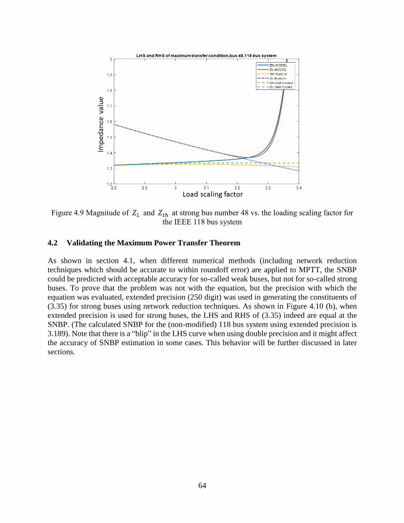
64

Figure 4.9 Magnitude of 𝑍𝐿 and 𝑍𝑡ℎ at strong bus number 48 vs. the loading scaling factor for

the IEEE 118 bus system

4.2 Validating the Maximum Power Transfer Theorem

As shown in section 4.1, when different numerical methods (including network reduction

techniques which should be accurate to within roundoff error) are applied to MPTT, the SNBP

could be predicted with acceptable accuracy for so-called weak buses, but not for so-called strong

buses. To prove that the problem was not with the equation, but the precision with which the

equation was evaluated, extended precision (250 digit) was used in generating the constituents of

(3.35) for strong buses using network reduction techniques. As shown in Figure 4.10 (b), when

extended precision is used for strong buses, the LHS and RHS of (3.35) indeed are equal at the

SNBP. (The calculated SNBP for the (non-modified) 118 bus system using extended precision is

3.189). Note that there is a “blip” in the LHS curve when using double precision and it might affect

the accuracy of SNBP estimation in some cases. This behavior will be further discussed in later

sections.

65

(a) Double precision

(b) 250 digits of precision


IEEE 118 bus system

66

4.3 Numerical comparison of different methods using noiseless measurements

In the above section, the MPTT was validated by implementing it using high precision and, in

section 4.1, different numerical methods were investigated to estimate the SNBP based on the

MPTT from measurements. However, it was shown that, regardless of the method used, when only

double precision is used the method cannot predict the SNBP using data from strong buses. Hence,

to be effective, SNBP prediction algorithm should be applied to PMU buses that are close to the

weakest buses in the system. Also it was observed from the above numerical experiments that the

Built-In, Self-Coded and Best Component methods are promising if applied to weak buses, but a

larger performance sample will aid in drawing a conclusion with high confidence. Therefore, more

extensive tests were conducted using these three methods with 11 weak buses on the 118 bus

system in the following sections.

4.3.1 Modified 118 bus system

The tested 118 bus system is modified by adding a small load, S=1+1jMVA, to bus 30, bus 37 and

bus 38 in order to increase the number of testable weak buses in the system. (Because there is no

real or reactive power load at those PQ buses in the original system, the MPTT could not be applied

to those buses.) The loading value at the SNBP for this modified 118 bus system is 3.172 (versus

3.189 for the original system), obtained using the CPF.

4.3.2 Finding the ten weakest buses from modal analysis

Arguably, the most well-known method of determining the weak buses of a system is modal

analysis [29], which will be used here to determine the ten weakest buses of the modified 118 bus

system.

The modal analysis method calculates the eigenvalue and eigenvector of the reduced Jacobian

matrix based on the relation between the incremental bus voltage magnitudes and their respective

incremental reactive power injections. The smallest eigenvalue can be used to estimate the stability

margin and the participation factor calculated from the left and right eigenvectors corresponding

to the critical mode, which provides insight about which bus loads have significant impact on the

system voltage stability. The buses with relatively large participation factors in the smallest

eigenvalue are determined to be the weak buses in the system. Since modal analysis is based on a

linear approximation of the system model, the order of the buses from the weakest to the strongest

might change as the operating condition changes.

The top ten weakest buses (in decreasing order of weakness) obtained from modal analysis using

VSAT [35] and our own MATLAB modal-analysis program for the modified 118 bus system are

listed in Table 4.3, both calculated when the loading of the system is close to its SNBP. Note that

when using VSAT to identify the weakest buses, we can only scale the system load up to 2.35

because VSAT can not give a converged solution beyond that. It can be observed that there is a

one-to-one correspondence between VSAT and MATLAB program except for the 10th weakest

bus, i.e., the strongest one among the 10 weakest buses. Thus, this shows that, in this case, the

order of the top ten weakest buses changes only slightly as the loading changes. The first nine

67

weakest buses ( identical for VSAT and MATLAB) and the 10th weakest buses both for VSAT

and MATLAB, totaling eleven buses, are selected to be tested in the following section.

Table 4.3 Ten weakest buses for the modified 118 bus system using modal analysis

VSAT (loading=2.35) MATLAB (loading=3)

Smallest

eigenvalue 2.947722 3.035

No. Bus Part.Fac. Bus Part.Fac

1 21 1 21 1

2 22 0.80834 22 0.83712

3 20 0.47027 20 0.46517

4 44 0.05503 44 0.04171

5 43 0.02785 43 0.0195

6 45 0.01984 45 0.01658

7 23 0.01407 23 0.01603

8 38 0.00313 38 0.00218

9 30 0.0006 30 0.00085

10 37 0.00016 17 0.00012

4.3.3 Numerical results

Numerical tests were conducted on the Built-In, Self-Coded and Best Component methods for the

eleven weakest buses in the modified 118 bus system with different ranges of noiseless pseudo-

measurements. In each experiment, 200 measurements were used to fit a [30/30] Padé approximant

for each variable. The SNBP was predicted either by the crossover or divergence behavior of the

LHS and RHS values of the MPTT equation.The numerical results are shown as follows, where

“Average error” is the average of the absolute value of the errors:

4.3.3.1 Measurements in the range of 50%-60% of the SNBP

In this experiment, the measurements in the 50%-60% training range were used to fit the Padé

approximant. The percent error in SNBP for the 11 weakest buses using the three numerical

methods are listed in Table 4.4 and the absolute value of the errors is shown in Figure 4.11.

68

Table 4.4 Percent error in SNBP estimation for measurements in the 50%-60% training range for

the modified 118 bus system

Bus no. Numerical methods

Average error over all

methods (%) Built-In (%) Self-Coded

(%)

Best Compo-

nent (%)

21 4.17087 6.882093 8.237705 6.430223

22 12.16898 2.301387 2.04918 5.506515

20 2.175284 9.174023 6.052963 5.800757

44 -1.25158 0.29319 -0.05359 0.532787

43 -0.02207 0.576923 0.608449 0.40248

45 -1.8285 5.422446 5.453972 4.234973

23 -5.64313 12.54729 13.11475 10.43506

38 -2.60404 -0.81021 -1.50378 1.639344

30 0.063052 5.611602 -3.97226 3.215637

37 -0.90479 6.472257 7.796343 5.057797

17 -2.71122 13.52459 18.63178 11.62253

Average error

over all buses 3.04941 5.783274 6.134071 4.988918


0

2

4

6

8

10

12

14

16

18

20

bus 21 bus 22 bus 20 bus 44 bus 43 bus 45 bus 23 bus 38 bus 30 bus 37 bus 17

SNB

P e

stim

atio

n e

rro

r%

Built-In Self-Coded Best Component

69


The numerical results of SNBP estimation using measurements in the 60%-70% training range are

shown in Table 4.5 and Figure 4.12.






(%)

Best Compo-

nent (%)

21 6.431274 4.854981 7.124842 6.137032

22 0.189155 -0.09458 -0.15763 0.147121

20 10.40353 8.228247 8.732661 9.12148

44 -8.62863 0.955233 1.144388 3.576082

43 0.797604 2.689155 2.058638 1.848466

45 -2.60404 0.513871 0.513871 1.210593

23 -14.029 4.287516 7.093317 8.469945

38 0.545397 -2.60404 -2.60404 1.917823

30 -5.42245 4.602774 3.87768 4.6343

37 2.657629 3.225095 3.571879 3.151534

17 2.900378 9.962169 8.417402 7.093317

Average error

over all buses 4.964462 3.819787 4.117849 4.300699

70



The numerical results of the SNBP estimation using measurements in the 70%-80% training range

are shown in Table 4.6 and Figure 4.13.

0

2

4

6

8

10

12

14

16


SNB

P e

stim

atio

n e

rro

r%


71






(%)

Best Compo-

nent (%)

21 0.094578 -0.44136 -0.50441 0.346784

22 1.481715 1.261034 0.031526 0.924758

20 1.680328 1.806431 0.040984 1.175914

44 -0.49496 -1.44073 -1.59836 1.178016

43 1.081337 -0.02207 -0.24275 0.448718

45 0.513871 0.040984 0.040984 0.198613

23 2.909836 1.869483 1.995586 2.258302

38 -0.36885 -0.46343 -0.58953 0.473939

30 0.135561 -0.84174 -0.84174 0.606347

37 0.671501 1.20744 1.302018 1.060319

17 2.373897 1.428121 1.428121 1.74338

Average error

over all buses 1.073312 0.983893 0.783274 0.946826


0

0.5

1

1.5

2

2.5

3

3.5

bus 21bus 22bus 20bus 44bus 43bus 45bus 23bus 38bus 30bus 37bus 17

SNB

P e

stim

atio

n e

rro

r%

Buit-In Self-Coded Best Component

72

4.3.4 Conclusion

From the above numerical results, it can be observed that the average errors in SNBP estimation

using the three different methods are: 3%-6% for measurements in the 50%-60% range; 3%-5%

for measurements in the 60%-70% range; about 1% for measurements in the 70%-80%. If simply

taking the average of the average of the absolute values of the errors for the three methods, the

approximate errors for each training data range are shown in Figure 4.14. It can be seen that the

closer the measured data is to the SNBP, the smaller is the error in the SNBP estimate.

Figure 4.14 Percent error in SNBP estimation for different training data range (average of the ab-

solute value of errors)

If we average over the 11 weakest buses (no absolute value), the Built-In method gives the best

results as shown in Figure 4.15. Other methods may be competitive if more sophisticated algo-

rithms of outlier detection are used.

3.04941

4.96446

1.073312

0

1

2

3

4

5

6

50%-60% 60%-70% 70%-80%

SNBP estimation error (Average) %

73

Figure 4.15 Percent error in SNBP estimation for different training data range (average errors)

4.3.5 More analysis on the numerical results

When the range of the measurements is 60%-70% of the SNBP, the numerical results as shown in

Figure 4.12 show that the errors in SNBP estimation using the Built-In method for most buses are

less than 7%, which is acceptable. However, the estimation error at bus 23 is 14.029%. (The esti-

mated SNBP is 2.727 while the true SNBP of the system is 3.172), which obviously is an outlier.

Hence, in order to improve the accuracy of our method for estimating the SNBP, we focus now on

finding the cause of this outlier. Bus 43, for which the estimation error is only 0.797%, is also

included in the following tests for comparison.

If we generate the MPTT plot for bus 23 as shown in Figure 6.23 (a), it can be observed that the

yellow line which represents the LHS of (3.35) has a spike at around 2.727 and this point will be

detected as the SNBP by the divergence criteria, which is incorrect. Then by analyzing each com-

ponent in the LHS of (3.35) (∂|𝑉𝑠|2, 𝜕𝑅𝐿(𝛼), 𝑅𝐿(𝛼) and |𝑉𝑠|2), we find that the cause comes from

∂|𝑉𝑠|2 as shown in Figure 6.24 (a).

-1

0

1

2

3

4

5

6

50%-60% 60%-70% 70%-80%

SNBP estimation error%


74

(a) Bus 23 (b) Bus 43

Figure 4.16 LHS and RHS of (3.35) at bus 23 or bus 43 vs. loading scaling factor

(a) Bus 23 (b) Bus 43

Figure 4.17 𝜕|𝑉𝑠(𝛼)|2 at bus number 23 or bus 43 vs. loading-scaling factor

To dive further into determining the root cause of blip in Figure 6.24 (a), the poles and zeros of

the Padé approximants of ∂|V𝑠|2for bus 23 and bus 43 are plotted in Figure 4.18. It can be seen

that there are a number of poles/zeros accumulating on the real axis in the range [1.9, 2.22], which

is the measured data range. Since we only focus on the range beyond the measured data range for

estimating the SNBP, these poles/zeros will not affect the estimation. And the pole/zero that is

located at around 3.4 should be the actual root of the Padé approximant obtained from measure-

ments and will be taken as the estimated SNBP if using the roots method. (Using the roots method,

an estimated SNBP of 3.4 is significantly inaccurate, which is why the MPTT is used.) Observe

that for bus 23, there is a pole-zero pair in the range between the boundary of the measured data

range and the root of the Padé approximant, located at around 2.73 (also inaccurate if the roots

method were to be used) and this pole-zero pair will affect the behavior of the LHS and RHS of

(3.35). Therefore, when we search for the estimated SNBP detected by crossover or divergence

behavior starting from the boundary of the measured data range, the estimation of the SNBP is

75

2.727, which is incorrect. More discussion on the poles and zeros of the Padé approximant obtained

from measurements is contained in section 4.4, as well as suggested remedies for this problem. As

will be seen in section 4.4, this pole-zero pair for bus 23 is caused by round-off error.

(a) Bus 23 (b) Bus 43

Figure 4.18 Pole-zero plot for 𝜕|𝑉𝑠(𝛼)|2 at bus number 23 and bus 43

4.4 Using the roots method to estimate the SNBP

In addition to using the MPTT, one can use the roots (poles/zeros) of the voltage Padé approximant

to estimate the SNBP using the so-called roots method. As seen in section 4.3.5, the location of

the poles/zeros of the Padé approximant is an effective way to analyze numerical issues. Hence

the numerical performance of the roots method will be discussed in the following section.

4.4.1 The effect of order of Padé approximant

The pole-zero plots for different orders of [M/M+1] Padé approximants of 𝑉𝐿 at bus 23 are plotted

in Figure 4.19 using various numbers of series terms, n. The range of the measurements used to fit

the Padé approximant is 60%-70% of the SNBP, which is 1.9032 to 2.2204 in 𝛼 values. The total

number of measurements is 200. It is seen from Figure 6.26 (a) that when the number of terms, 𝑛,

used to calculate the Padé approximants is insufficient, like n=4 in this case, there is no pole/zero

on the real axis and thus no SNBP prediction can be made using the roots method. Looking at

Figure 6.26 (b) (c) and (d),we observe that the pole/zero that is located at around 3.4 is viewed to

be the actual root of Padé approximants of 𝑉𝐿 fitted from measurements and will be referred to

“the meaningful” pole/zero in the rest of the work. It was observed that the location of the mean-

ingful pole/zero changes slightly as n changes. However, as n increases, beyond a certain thresh-

old, as seen in Figure 6.26 (c), poles/zeros occur on the real axis inside and just beyond the training

data range, i.e., [1.9032, 2.2204]. This type of poles/zeros will be referred to “training range”

poles/zeros. When n=20, those training range poles/zeros are all within the training data range and

thus will not affect the accuracy of the SNBP estimation. When n increases to 50, as shown in

Figure 6.26 (d), many poles/zeros accumulating on a circle centered at the origin, which will be

referred to as “the circle” poles/zeros in the following sections. Also, observe in Figure 6.26 (d)

that there is an (approximately real-valued) near-training-range pole/zero located at 2.312, which

76

is beyond the training data range and would be taken as the estimated SNBP from roots method,

leading to inaccuracy in SNBP prediction.

(a) n=4 (b) n=10

(c) n=20 (d) n=50

Figure 4.19 Pole-zero plot for different order of 𝑉𝐿 Padé approximant

Let us define the following variables.

• 𝑁𝑠𝑡𝑎𝑟𝑡 is the number of terms at which the Padé approximant starts to have a pole/zero on

or near the real axis, which consequently would allow the prediction of the SNBP by the

roots method (as seen in Figure 6.26 (b)) to be reasonably accurate,

• 𝑁𝑟𝑎𝑛𝑔𝑒 is the number of terms at which the Padé approximant starts to have training range

poles/zeros all in the training range but these roots remain within the training range so they

do not affect the accuracy of the SNBP estimation (as seen in Figure 6.26 (c))

• 𝑁𝑏𝑎𝑑 corresponds to the number of terms of the Padé approximant when there exist train-

ing range poles/zeros located beyond the training data range as more and more spurious

poles/zeros appear, thus causing estimation errors (as seen in Figure 6.26 (d)).

77

The general conclusion from a series of tests on the modified 118 bus system is that in general:

𝑁𝑠𝑡𝑎𝑟𝑡 = 7, 𝑁𝑟𝑎𝑛𝑔𝑒 = 12 and 𝑁𝑏𝑎𝑑 = 21. The specific SNBP estimation results for bus 23 are

shown in Figure 4.20.

Figure 4.20 The estimation of SNBP vs. number of series terms used in building the Padé ap-

proximant of 𝑉𝐿 using 200 measurements

As seen from Figure 4.20, one does not need many terms to obtain a reasonably accurate estimate

of the SNBP and using too many terms will reduce the accuracy of the estimation eventually.

Typically, n=12 to 20 will give a reasonably good SNBP estimation.

4.4.2 The effect of number of measurements

As demonstrated in section 4.1.1, the Padé approximant is calculated by solving a set of overde-

termined equations. Increasing the number of measurements is expected to reduce round-off error.

If we repeat the simulation in section 4.4.1 with 2000 measurements, the result we obtain is:

𝑁𝑠𝑡𝑎𝑟𝑡 = 5, 𝑁𝑟𝑎𝑛𝑔𝑒 = 18 and 𝑁𝑏𝑎𝑑 = 24, which means we can use a wider range of n selections

and still obtain a good estimate. The specific SNBP estimation results are shown in Figure 4.21.

Notice that the SNBP estimate is more reliable when 2000 samples are used versus 200 samples,

as shown in Figure 4.20.

0

0.5

1

1.5

2

2.5

3

3.5

4

2 3 4 5 6 7 8 9 10 11 12 13 14 15 16 17 18 19 20 21 25 30 35 40 45 50 55 61

SNBP estimation VS Nterm

SNBP estimation True SNBP (3.172)

78

Figure 4.21 The estimation of SNBP vs. number of series terms used in building the Padé ap-

proximant of 𝑉𝐿 using 2000 measurements

4.4.3 The effect of precision

As shown in Figure 4.20, we classify three types of poles/zeros of the Padé approximant by their

locations: meaningful pole/zero, training range pole/zero, and circle pole/zero. To have a better

understanding of which factors affect the locations of those roots, we implemented a high precision

code that we used to perform the following tests. We recognized that spurious roots could be

caused by errors in either the measurements or the calculation of the Padé approximant. Therefore,

we implemented our training algorithm with different numbers of digits of precision in both ob-

taining the pseudo-measurements and fitting the Padé approximants. The simulation results are

shown in Figure 4.22, Figure 4.23, and Figure 4.24. The number of terms used here is 50.

0

0.5

1

1.5

2

2.5

3

3.5

4

2 3 4 5 6 7 8 9 10 11 12 13 14 15 16 17 18 19 20 21 25 30 35 40 45 50 55 61

SNBP estimation VS Nterms (bus 23)

SNBP estimation (Nmeasure=2000) True SNBP (3.172)

79


precision measurements, double precision Padé approximant)


precision measurements, 220 digits of precision Padé approximant)

80

Figure 4.24 Pole-zero plot for 𝑉𝐿 Padé approximant for the modified 118 bus system (220 digits

of precision measurements, 220 digits of precision Padé approximant)

By comparing Figure 4.22 and Figure 4.23, we can see that the circle poles/zeros disappear when

using high precision to fit the Padé approximants. Therefore, the circle poles/zeros are in fact spu-

rious roots due to round-off errors during the calculation of the Padé approximant coefficients.

Note that the circle poles/zeros in Figure 4.22 seem to move to the training data range as shown in

Figure 4.23 and the location of the meaningful poles/zeros does not change much when using high

precision to fit the Padé approximants.

By comparing Figure 4.23 and Figure 4.24, we can see that the training range poles/zeros disappear

if both measurements and Padé approximants are calculated with high precision. In addition, the

meaningful poles/zeros are closer to the true SNBP of the system (the meaningful pole/zero is

located at 3.34 and 3.172 in Figure 4.23 and Figure 4.24 respectively). Therefore, we can conclude

that the occurrence of those training range poles/zeros comes from measurement errors. Also, ob-

taining a more accurate estimation of the meaningful pole requires using high precision for both

measurements as well as Padé approximants. Given that precision is limited from PMU measure-

ments (maybe 3-4 accurate digits, if noise is minimal), accurately predicting the SNBP from meas-

ured data will require more elaborate means than the simple roots method.

In summary, in order to improve the accuracy of roots method for estimating the SNBP, one should

focus on reducing measurement noise or eliminating spurious poles/zeros caused by the computa-

tion of Padé approximants.

81

4.4.4 Comparison of the MPTT and the roots method

The comparison of SNBP estimation error produced by the MPTT using the Built-In method and

the roots method was performed using the eleven weakest buses for the modified 118 bus system.

The measurements in the 60%-70% range were used to fit the Padé approximant, obtained using

MATPOWER with a power-mismatch convergence tolerance of 10-8. The numerical results are

shown in Figure 4.25 where mp120 represents using 120 digits of precision to fit the Padé approx-

imants. The error in the SNBP estimation is the average of the absolute errors for all buses shown

in Figure 4.25.

Figure 4.25 Comparison of MPTT and roots method for estimating the SNBP

From Figure 4.25 we can conclude that:

(1) The MPTT method can give more accurate results than the roots method for the system

test. The roots method is more sensitive to the number of terms and digits of precision

used for the Padé approximant.

(2) Reducing the order of Padé approximant (for example, using n=10 instead of n=60 in

this case) helps to eliminate estimation errors with the roots method and with the MPTT

method when using double precision.

(3) Increasing precision can improve accuracy, which is expected. But when we use a

small-order Padé approximant (n=10 for example), the effect of precision is not as sig-

nificant.

Therefore, generally, estimating the SNBP using the MPTT method with double precision and

n=10 for the Padé approximant seems to be a prudent choice. More numerical experiments on a

wide variety of systems is needed to confirm this hypothesis.

0

2

4

6

8

10

12

14

MPTT (double) MPTT (mp120) Roots method(double)

Roots method(mp120)

SNBP error% (no noise)

N=10 N=60

82

4.5 Numerical comparison of different methods using noisy measurements

4.5.1 Numerical results

We inserted random noise (zero mean, standard deviation of 0.01) in a range of PMU voltage

pseudo-measurements from the modified 118 bus system and repeated the same numerical tests as

presented in section 4.3. The numerical results we obtained are shown in Table 4.7 and Figure

4.26. The average error in SNBP estimation for a 70%-80% training range is around 15%, which

is unacceptable. The poles/zeros of the Padé approximant for bus 23 are plotted in Figure 4.27. It

is observed that there are no meaningful poles/zeros in this plot because of the corruption of the

measurements by noise; therefore, neither the MPTT method nor the roots method works and more

research is needed in the future to develop different methods for ameliorating measurement error.

Table 4.7 Percent error in SNBP estimation for noisy measurements in the 70%-80% training

range for the modified 118 bus system




(%)

Best Compo-

nent (%)

21 -19.4515 -19.1362 -16.6141 18.40059

22 -19.4515 -17.8752 -19.4515 18.92602

20 -19.1362 17.74905 -4.6343 13.83985

44 11.44388 -15.0378 -15.3531 13.94493

43 -13.4615 -7.47163 -11.2547 10.7293

45 -19.4515 -19.4515 -19.1362 19.34636

23 -16.2989 -7.78689 -19.4515 14.5124

38 -17.2446 -19.4515 -19.4515 18.71585

30 -11.57 -19.4515 6.399748 12.47373

37 -15.6683 -18.8209 -19.4515 17.98024

17 -10.6242 -0.8512 -15.9836 9.153005

Average error

over all buses 15.80018 14.82575 15.19833 15.27475

83

Figure 4.26 Percent error in SNBP estimation for noisy measurements in the 70%-80% training

range

Figure 4.27 Pole-zero plot for 𝑉𝐿 Padé approximant with noisy measurements

0

5

10

15

20

25


SNB

P e

stim

atio

n e

rro

r%

Percent error in SNBP estimation

Build-In Pade Fit Self-Coded PadenFit Best Component

84

4.5.2 Analytic Derivative method

In the above tests, the components ∂|𝑉𝑠(𝛼)|2and 𝜕𝑅𝐿 in the MPTT were obtained by directly fit-

ting the corresponding Padé approximant from the corresponding numerically calculated incre-

mental values, i.e., the numerically calculate voltage and load resistance increments (i.e., subtrac-

tion of adjacent measurements), respectively. Even relatively small deviations in these measure-

ments from the true values (due to measurement noise) will have a large effect on the value of the

increment, and therefore on the derivative. To eliminate the use of the numerically calculated in-

cremental values, another fitting technique was developed, specifically the “Analytic Derivative”

method, introduced next.

In the Analytic Derivative method, rather than taking the derivative numerically by subtracting

adjacent measurements, the Padé approximant of the needed function is first constructed and then

the derivative of this function is performed analytically. For example, the Padé approximant for

∂|𝑉𝑠(𝛼)|2 is obtained by first fitting the Padé approximant to |𝑉𝑠(𝛼)|2 from the square of the

magnitude of the source voltage measurements and then taking the derivative of this rational func-

tion. The approach to getting the Padé approximant for 𝜕𝑅𝐿 is similar. The MPTT results using

the Analytic Derivative method for weak bus 22 in the modified 118 bus system from noiseless

measurements is plotted in Figure 4.28 and compared with the results from the Built-In method.

The measurement range is 60%-70% of the SNBP load, i.e., in the range 1.9032<<2.2204. It

is shown that the Analytic Derivative method does not perform as well as the Built-In method

because the LHS of the MPTT for the Analytic Derivative method deviates more from the true

curve earlier than the Built-In method. It is believed that performance is inferior in cases with

noiseless measurements because the process of taking the derivative for ∂|𝑉𝑠(𝛼)|2 and 𝜕𝑅𝐿 pro-

duces roundoff error.


modified 118 bus system using noiseless measurements

85

Next, we inserted random noise (zero mean, standard deviation of 10−9 and 10−6) into the volt-

age measurements and repeated the above numerical tests. The MPTT results using noisy meas-

urements with a standard deviation of 10−9 and 10−6 are shown in Figure 4.29 and Figure 4.30,

respectively. We can see that when using measurements with noise, the Analytic Derivative

method performs better than the Built-In method because it avoids the use of numerically calcu-

lated incremental values. However, this method is still not able to estimate the SNBP with accepta-

ble accuracy. More effort is needed to improve the numerical performance.


modified 118 bus system using noisy measurements with standard deviation of 10-9

86


modified 118 bus system using noisy measurements with standard deviation of 10-6

4.5.3 Summary

From above tests, we see that the noise in the measurements (whether injected, or inherent as

roundoff error in the calculation of the pseudo-measurements) has a similar effect on poles/zeros

as roundoff error (generated in the calculation of the Padé approximant). They lead to spurious

roots in the Padé approximant and affect the accuracy of the non-spurious poles/zeros and the

accuracy of the SNBP prediction. It is important to develop methods to eliminate the effect of

noise, which is left as future work.

4.6 Summary

This chapter concentrates on the application of HEM to the estimation of the SNBP using local

measurements. We developed a nonlinear Thévenin-like network from HE reduction and establish

the Maximum Power Transfer Theorem for estimating the SNBP, which has been validated using

high precision. Different numerical methods are investigated and the comparison of their numeri-

cal performance is conducted on a modified version of the IEEE 118 bus system using measure-

ments with/without noise. We also looked at the poles/zeros of the Padé approximant to analyze

the source of estimation error. We found that spurious pole/zero pairs caused by measurement

error and roundoff error impacted accuracy. Developing different ways to minimize the effect of

noise is necessary and is left for future work.

87

5. Conclusions

The local-measurement-based methods of estimating the SNBP using linear Thévenin networks

were explored along with the possible impacts of discrete changes on such methods. HE-reduction

was used to develop nonlinear Thévenin-like networks for which the maximum power transfer

condition was derived and verified. It was shown that, for such Thévenin-like networks as well as

nonlinear multi-bus reduced-order networks, the topology and impedances of the reduced network

can be arbitrarily assumed and measurements be used to fit the polynomials for the nonlinear volt-

age source/current injections. A revised sigma index was obtained using the nonlinear Thévenin-

like network, however it was seen that it cannot be used in raw form to estimate the weak buses in

the system. Whether the sigma index can be used in some form to identify weak buses remains an

open problem.

The theory for building nonlinear networks from PMU measurement of the bus-voltage and then

using the MPTT and the roots method to predict the SNBP was developed. The performance of

some of the proposed numerical methods worked acceptably on noiseless pseudo-measurements.

When these methods were used with pseudo-measurements that were corrupted with noise the

performance was less accurate than hoped. Methods for improving the performance are suggested

in the report.

88

References

[1] A. Trias, “The holomorphic embedding load flow method,” IEEE Power and Energy Society

General Meeting, July 2012, pp. 1-8.

[2] S. D. Rao, D. J. Tylavsky, and Y. Feng, “Estimating the saddle-node bifurcation point of static

power systems using the holomorphic embedding method,” International Journal of Electrical

Power & Energy Systems, vol. 84, pp. 1-12, 2017.

[3] R. J. Avalos, C. A. Cañizares, F. Milano, and A. J. Conejo, “Equivalency of continuation and

optimization methods to determine saddle-node and limit-induced bifurcations in power sys-

tems,” IEEE Transactions on Circuits and Systems I: Regular Papers, vol. 56, no. 1, pp. 210-

223, 2009.

[4] D. R. Gurusinghe, “Saddle Node Bifurcation and Voltage Stability Analysis of Sri Lanka,”

Engineer: Journal of the Institution of Engineers, Sri Lanka, vol. 45, no. 4, 2012.

[5] V. Ajjarapu and C. Christy, “The continuation power flow: a tool for steady state voltage sta-

bility analysis,” IEEE transactions on Power Systems, vol. 7, no. 1, pp. 416-423, 1992.

[6] E. Garbelini, D. A. Alves, A. B. Neto, E. Righeto, L. C. da Silva, and C. A. Castro, “An effi-

cient geometric parameterization technique for the continuation power flow,” Electric Power

Systems Research, vol. 77, no. 1, pp. 71-82, 2007.

[7] E. d. M. Magalhães, A. Bonini Neto, and D. A. Alves, “A parameterization technique for the

continuation power flow developed from the analysis of power flow curves,” Mathematical

Problems in Engineering, vol. 2012, 2012.

[8] A. B. Neto and D. Alves, “Improved geometric parameterisation techniques for continuation

power flow,” IET generation, transmission & distribution, vol. 4, no. 12, pp. 1349-1359, 2010.

[9] A. Jalali, M. Aldeen, “Novel continuation power flow algorithm”, IEEE PES International

Conference on Power Systems Technology (POWERCON), 2016.

[10] P. Xu, X. Wang, and V. Ajjarapu, “Continuation power flow with adaptive stepsize control

via convergence monitor,” IET generation, transmission & distribution, vol. 6, no. 7, pp. 673-

679, 2012.

[11] D. A. Alves, L. C. da Silva, C. A. Castro, and V. F. da Costa, “Continuation fast decoupled

power flow with secant predictor,” IEEE transactions on Power Systems, vol. 18, no. 3, pp.

1078-1085, 2003.

[12] S. H. Li and H. D. Chiang, “Continuation power flow with multiple load variation and gen-

eration re-dispatch patterns,” in Power Engineering Society General Meeting, 2006.

[13] K. Vu, M. M. Begovic, D. Novosel, and M. M. Saha, “Use of local measurements to estimate

voltage-stability margin,” IEEE Transactions on Power Systems, vol. 14, no. 3, pp. 1029-

1035, 1999.

[14] D. Julian, R. P. Schulz, K. Vu, W. H. Quaintance, N. B. Bhatt, and D. Novosel, “Quantifying

proximity to voltage collapse using the voltage instability predictor (VIP),” in Power Engi-

neering Society Summer Meeting, 2000. IEEE, 2000, vol. 2, pp. 931-936: IEEE.

[15] I. Smon, G. Verbic, and F. Gubina, “Local voltage-stability index using Tellegen's theorem,”

IEEE Transactions on Power Systems, vol. 21, no. 3, pp. 1267-1275, 2006.

[16] S. Corsi and G. N. Taranto, “A real-time voltage instability identification algorithm based on

local phasor measurements,” IEEE transactions on power systems, vol. 23, no. 3, pp. 1271-

1279, 2008.

89

[17] H. Yuan and F. Li, “A comparative study of measurement-based Thevenin equivalents iden-

tification methods,” in North American Power Symposium (NAPS), 2014, 2014, pp. 1-6:

IEEE.

[18] EPRI Technical Update: Voltage Instability Load Shedding. EPRI, Palo Alto, CA: 2006.

1012491.

[19] M. Zima, M. Larsson, P. Korba, C. Rehtanz, and G. Andersson, “Design aspects for wide-

area monitoring and control systems,” Proceedings of the IEEE, vol. 93, no. 5, pp. 980-996,

2005.

[20] G. Huang, L. Zhao, “Measurement Based Voltage Stability Monitoring of Power System,”

PSERC publication 2001, available online: www.pserc.wisc.edu, 2001

[21] M. Larsson, C. Rehtanz, J. Bertsch, “Real-Time Voltage Stability Assessment of Transmis-

sion Corridors,” Proc. IFAC Symposium on Power Plants and Power Systems, Seoul, S. Ko-

rea, 2003

[22] J.-H. Liu and C.-C. Chu, “Wide-area measurement-based voltage stability indicators by mod-

ified coupled single-port models,” IEEE Transactions on Power Systems, vol. 29, no. 2, pp.

756-764, 2014.

[23] S. G. Ghiocel et al., “Phasor-measurement-based voltage stability margin calculation for a

power transfer interface with multiple injections and transfer paths,” in Power Systems Com-

putation Conference (PSCC), 2014, 2014, pp. 1-6: IEEE.

[24] F. Hu, K. Sun, A. Del Rosso, E. Farantatos, and N. Bhatt, “Measurement-based real-time

voltage stability monitoring for load areas,” IEEE Transactions on Power Systems, vol. 31,

no. 4, pp. 2787-2798, 2016.

[25] B. Milosevic, M. Begovic, “Voltage-stability protection and control using a wide-area net-

work of phasor measurements,” IEEE Trans. Power Systems, vol. 18, no. 1, pp. 121-127,

2003.

[26] M. Glavic and T. V. Cutsem, “A Short Survey of Methods for Voltage Instability Detection,”

Proceedings of the IEEE PES General Meeting, Detroit, July 2011.

[27] Y. Zhu, D. Tylavsky, and S. Rao, “Nonlinear structure-preserving network reduction using

holomorphic embedding,” IEEE Transactions on Power Systems, vol. 33, no. 2, pp. 1926-

1935, 2018.

[28] S. Rao and D. Tylavsky, “Nonlinear network reduction for distribution networks using the

holomorphic embedding method,” in North American Power Symposium (NAPS), 2016,

2016, pp. 1-6: IEEE.

[29] P. Kundur, N. J. Balu, and M. G. Lauby, Power system stability and control. McGraw-hill

New York, 1994.

[30] P. Gonnet, S. Suttel, and L. N. Trefethen, “Robust Padé Approximation via SVD,” SIAM

Review, vol. 55, no. 1, pp. 101-117, 2013.

[31] Shruti Rao, Yang Feng, Daniel Tylavsky and Muthu Kumar Subramaniam, “The Holomorphic

Embedding Method Applied to the Power-Flow Problem,” IEEE Transactions on Power Sys-

tems , vol. 31, no. 5, pp. 3816-3828, Sept. 2016.

[32] C. A. Canizares and F. L. Alvarado, “Point of collapse and continuation methods for large

AC/DC systems,” IEEE Transactions on Power Systems, vol. 8, no. 1, pp. 1-8, Feb 1993.

[33] A. Trias, “Sigma algebraic approximants as a diagnostic tool in power networks,” US Patent

2014/0156094 (2014).

[34] R. D. Zimmerman, C. E. Murillo-Sánchez and R. J. Thomas, “MATPOWER: Steady-State

Operations, Planning and Analysis Tools for Power Systems Research and Education,” IEEE

http://dx.doi.org/10.1109/TPWRS.2010.2051168

http://dx.doi.org/10.1109/TPWRS.2010.2051168

90

Transactions on Power Systems, Feb. 2011, vol. 26, no. 1, pp. 12-19.

[35] “Voltage Security Assessment Tool,” DSATools, accessed in April 2015, available at:

http://www.dsatools.com/html/prod_vsat.php.

[36] J. S. Giraldo, J. A. Castrillon and C. A. Castro, “Network-free voltage stability assessment of

power systems using phasor measurements,” 2015 IEEE Eindhoven PowerTech, Eindhoven,

2015, pp. 1-5.

[37] S. A. Soliman, H. K. Temraz and S. M. El-Khodary, “Power system voltage stability margin

identification using local measurements,” Large Engineering Systems Conference on Power

Engineering, 2003, 2003, pp. 100-104.

[38] M. Parniani, J. H. Chow, L. Vanfretti, B. Bhargava, A. Salazar, “Voltage Stability Analysis

of a Multiple-Infeed Load Center Using Phasor Measurement Data,” Proc. 2006 IEEE Power

System Conference and Exposition, Atlanta, GA, Oct./Nov. 2006.

[39] P. Zhang, L. Min, N. Zhang, “Voltage Instability Load Shedding,” EPRI Report 1012491,

Sep. 2006.

[40] Illinois Center for a Smarter Electric Grid (ICSEG), “IEEE 14-Bus System,” accessed, April

2017, available at: http://icseg.iti.illinois.edu/ieee-14-bus-system/

[41] S. S. Biswas, C. B. Vellaithurai and A. K. Srivastava, “Development and real time

implementation of a synchrophasor based fast voltage stability monitoring algorithm with

consideration of load models,” 2013 IEEE Industry Applications Society Annual Meeting,

Lake Buena Vista, FL, 2013, pp. 1-9.

[42] A. Perez, H. Jóhannsson, J. Østergaard, M. Glavic and T. Van Cutsem, “Improved Thévenin

equivalent methods for real-time voltage stability assessment,” 2016 IEEE International

Energy Conference.

[43] K. Sun, F. Hu and N. Bhatt, “A new approach for real-time voltage stability monitoring using

PMUs,” 2014 IEEE Innovative Smart Grid Technologies - Asia (ISGT ASIA), Kuala

Lumpur, 2014, pp. 232-237.

[44] D. Osipov, F. Hu and K. Sun, “Voltage stability margin estimation for a load area using a

three-bus equivalent,” 2016 IEEE Power and Energy Society General Meeting (PESGM),

Boston, MA, 2016, pp. 1-5.

[45] F. Hu, K. Sun, A. Del Rosso, E. Farantatos and N. Bhatt, “An adaptive three-bus power

system equivalent for estimating voltage stability margin from synchronized phasor

measurements,” 2014 IEEE PES General Meeting, Conference & Exposition, National

Harbor, MD, 2014, pp. 1-5.

[46] M. Nakmali, D. Osipov and K. Sun, “A new hybrid approach to thevenin equivalent

estimation for voltage stability monitoring, “ 2015 IEEE Power & Energy Society General

Meeting, Denver, CO, 2015, pp. 1-5.

[47] A. Wiszniewski, “New Criteria of Voltage Stability Margin for the Purpose of Load

Shedding, “ in IEEE Transactions on Power Delivery, vol. 22, no. 3, pp. 1367-1371, July

2007.

[48] I. Dobson and L. Lu, “Voltage collapse precipitated by the immediate change in stability

when generator reactive power limits are encountered,” IEEE Transactions on Circuits and

Systems I: Fundamental Theory and Applications, vol. 39, no. 9, pp. 762-766, Sep 1992.

[49] S. S. Baghsorkhi, S. P. Suetin, “Embedding AC Power Flow in the Complex Plane Part II: A

Reliable Framework for Voltage Collapse Analysis,” arXiv:1609.01211v1 [cs.SY], 2016.

[50] Zima M., Larsson M., Korba P., Rehtanz C., Andersson G., “Design aspects for wide-area

monitoring and control systems,” Proceedings of the IEEE, vol. 93, no. 5, pp. 980-996, 2005.

http://www.dsatools.com/html/prod_vsat.php

http://icseg.iti.illinois.edu/ieee-14-bus-system/

91

[51] S. Rao, D. Tylavsky, V. Vittal, W. Yi, D. Shi and Z. Wang, “Fast Weak-Bus and Bifurcation

Point Determination using Holomorphic Embedding Method,” 2018 IEEE Power & Energy

Society General Meeting (PESGM), Portland, OR, 2018, pp. 1-5.

Documents

Improving Voltage Stability Margin Estimation through the