Embed Size (px)
Citation preview

EARTBITNG ELECTRODES- POWER FREQUENCYA1:'-.TD\ IMPULSE BEHAVIOUR
DAN MORDECHAI EYTANI
A project report submitted to the Faculty of Engineering, University of theWitwatersrand, in partial fulfilment of the requirements for the degree ofMaster of Science in Engineering.
Johannesburg, 1995

DECLARATION
I declare that this project report is my own wade, the assistance which I havereceived is as follows:Assistance in construction of electrolytic tank and measurements in it.Construction of the test set-up at NETFA.HV measurements at NETFAassistance with step potential measurementsAssistance in typing and printing this reportThis project report is being submitted for the Degree of Master of Science inEngineering in the University of the Witwatersrand, Johannesburg. Ithas notbeen submitted before for any degree or examination in any other university.
T -Dan Mordechai Eytani
19th day of April 1995

ABSTRACT \\
Power frequency and Impulse tests were performed on earth electrodes,w'iich are being used in MV networks. The electrodes are combinations ofconductors buried in a trench and earth rods, which are driven verticallyinto the ground.
The power frequency tests included measurements of apparent electroderesistances and measurements of the surface equipotentials in the proximityof electrodes while they were carrying fault current. It was found that in anarea where the soil resistivity is decreasing with depth the use of long rodsreduced the low frequency electrode resistance significantly. Step potentialsaround the electrodes were quantified.
The impulse current distribution in the electrodes was measured and itwasfound that most of the current is dissipated from the rods. The reduction inelectrode resistance under impulse conditions was quantified for soil withresistivity of a few hundred ohms in the top layer dropping to 150-200 ohmsat depth of 3 meters. ':>'
The study provides a better understanding of the principles which should beapplied in the design of earth electrodes.

TO NrY PARENTS
RUTH ANTI SHMUEL BYTANII,
WITH .LOVE

v
ACKNOWLEDGEMENT
I would 1ikv to thank W Glynn and A Bekker (Johannesburg distributor -ESKOM) for providing the funds and allowing the time spent on thisproject.
lwould like [0 thank the following people for their contribution.towardsthis'proj ect:A Abrosie - Technology section JHB distributorH Fellows - Wits HV LaboratoryT Jacobs - Wits HV Laboratory!M Meyer - Technology section<.trm distributorA Muscat - WitsH Pinnar - HV measurements, TRIM'Roberts - HV measurements, TRIM Van Rensburg - HV Laboratory, SABSG Whyte - Technology section JHB distributor
Finally I would like to thank my supervisor Dr J Van Coller for hissound technical advice and guidance,

Hi
vi
PAGEiiiiiivvvivliiixxxi
1224555611
CONTENTS
DeclarationAbstractDedicationAcknowledgementsContentsList of figuresList of tablesList of SymbolsNomenclature
1. INTRODUCTION1.1 Earth electrodes - Power frequency1.1.1 Safety in earthing1.1.2 Protection operation1.2 Earth electrodes - Impulse behaviour1.2.1 Earth electrodes - Localized and Extended1.2.2 Electrical breakdown and ionization processes in soil1.2.3 Localized earth electrode - Dynamic models1.2.4 Extended earth electrode - Dynamic models
2.
2.12.1.12.1.22.22.2.12.2.22.32.4
3.
3.13.23.2~13.2.2
POWER FREQUENCY TESTS 13
Experimental set-up and Testing procedureStep potentials - field measurementsElectrolytic tank - Step potentialsPresentation of resultsfield measurementsElectrolytic tankInterpretation of resultsDiscussion
1313151616IS1820
IMPULSE TESTS 21
Experimental set up and testing procedurePresentation of resultsImpulse wave formsCurrent distribution
21
2325

vii
CONTENTS PAGE3.33.3.13.3.23.4
Interpretation of resultsReduction in electrode resistanceCurrent distributionDiscussion
26262727
4. CONCLUSIONS Al'4l> RECOMMENJ)ATIONS 28
4.14.2
Conclusions ItRecommendations for further work
2828
APPENDIX AAPPENDIX BAPPENDIX CAPPENDIX DAPPE:NlJIX E
FIELD MEASUREMENT RESt'lL TSELECTROLYTIC TANK RESuLTSTBST EQUIPMENTSOIL RESISTIVITY MEASUREMENTS. UVWHLSE TEST REStJL TS
AI-ASBI-B2
ClD1-D5E1 -E12
REFERENCES RI-R2

FIGURE
1.1
1.2
1.4
2.1
2.2
2.3
2.4
2.5
2.6
2.72.8
3.l
3.2
3.3
3.4
3.5
3.6
3.7
Cl
viii
Simplified model for resistance of single dri .en rod
Resistivity profiles in dynamic impulse resistance model
Equivalent circuit of surge current generator and impulse resistance
PAGE
7
8
9
Representation of ground electrode with uniformly distributed parameters 11
HV Lab and test site plan
Test set-up: Step potential and electrode resistance measurement
Step potential - method of measurement
Electrolytic tank test set-up
Measurement method
Surface equipotentials for electrode B
Surface equipotentials for electrode F
Earth electrode current and voltage vs electrode resistance
Test set-up: Impulse behaviour tests
Location of Rogowski coils for current distribution measurement
Generator output waveform
Voltage and total current at the electrode
Impulse currents at coil #4 and #7
Distribution of power frequency current - electrode A
Electrode resistance vs peak current
Rogowski coil - circuit diagram
13
14
14
15
16
17
18
20
21
22
23
24
25
26
Cl

TABLE2.1
2.2
3.1
3.2
ix
PAGEElectrode dimensions 13
Apparent low frequency resistance of'test electrode 17
Distribution of current in the earth electrodes
Power frequency current - proportional distribution 27

LIST OF SYMBOLS
d wire diameter, m.h buried depth of conductor, m,k empirical constant ( in body current calculation)1 rod length, m.r apparent electrode radius, m,rem maximura apparent copductor radius. m.ro electrode conductor radius, 1l1. •
s characteristic distance from center of electrode to the outermost point, m.t time, s.ts duration of current exposure, s.p soil resistivity, Qm .Po low current soil resistivity, Q In.
~1 ionization time constant, s.'!2 deionization time constant, S.A electrode surface area, m2•
Ec critical electrical field, kV1m.ESTEP step potentialETOUCH touch potentialG ground conductance per unit length, lin m .I current, A.IB body current, A.J current density, Al m2•
Jc critical current density, Al m2•
R resistance per unit length, Q/m .RB equivalent body resistance, Q.RE electrode resistance, Q.R2Fs series footing resistance, Q.R2Fp parallel footing resistance, Q.SF1! scaling factor for 11kV network voltage,SF22 scaling factor for 22kV network voltage.V volt/age,v.Z conventional impedance, ~'l:,Zo impulse impedance, Q.

xi
NOMENCLAT.!IRE
conventional ir..ipedance. The ratio between the maximum value of the total earthelectrode voltage and the peak value of the impulse current.
ground: A conducting connection, whether intentional or accidental, by which anelectric circuit or equipment is connected to the earth.
ground return t:~rcuit. A circuit in which the earth or an equivalent conducting body isutilized to complete the circuit and allow current circulation from or to its current source.
ground electrode. A conductor imbedded in the earth and used for collecting groundcurrent from or dissipating ground current into the earth.
ground potential rise (GPR). The maximum voltage that an earth electrode may attainrelative to a distant grounding point assumed to be aq:he potential of remote earth.
impulse impedance. The ratio between the instantaneous values of the total ground voltageof an earth electrode and of the total current at the injection point.
Rogowski coil. An open circuited, air-cored current transformer with a resistor-capacitor(Re) integrator on the secondary side - used for measurements of very high currents.
step potential. The difference in surface potential experienced by a person bridging adistance of 1m with his feet without contacting any other grounded object.
touch voltage. The potential difference between the ground potential rise(GPR) andthe surface potential at the point where person is standing, while at the same timehaving his hands in contact with a grounded structure.
transferred voltage. A special case of the touch voltage where a voltage is ..ssferredout of the area of the earth electrode.

1. iNTROD_PCTION
In R';mth Africa millions of t~ople still do not have electricity - this is the reason for the bigelectrification drive which is taking place throughout the country. A lot of work has beendone and a lot of work is currently in progress in order to ensure that the electrificationnetwork'S which will be 'Constructed will be cost effective without compromising theirperformance and safety.
Earthing is one of the most important factors, which effects both the performance of theelectrical network and its safety. This report deals with earth electrodes that are mainlyused on medium voltage (MV) networks. Two aspects were studied;a. Power frequency: electrode resistance to.true earth which is imponant for correct
protection operation. and surface potentials - the ~\~ety aspect.b. Impulse behaviour: the current distribution within the electrode and the reduction in
electrode resistance under impulse.
The aim of the study was to test various electrode configurations for their resistances andtheir surface equipotentials, as well as, their impulse behaviour - in order to get a betterunderstanding of the principles which should be applied in the design of earth electrodes.
This report considers two behaviours -fhe power frequency and the impulse behaviour.This introductory chapter includes two sections:
Section 1.1 gives the background on the safety aspects of earthing regarding thepermissible body currents, step and touch potentials, as well as a short review of theexpe . .mental work that was done in this field.
Section 1.2 gives the background on impulse behaviour of earthing electrodes. Theclassification of Ioralized earth electrodes and extended earth electrodes is explained, aswell as the electrical breakdown and ionization processes in the soil. Dynamic models oflocalized and extended earth electrodes are presented.
Chapter 2 covers the power frequency measurements and includes the experimental set-upand testing procedure, The step potential field measurements and the electrolytic tankmeasurements are presented and interpreted, followed by a discussion of the results.
Chapter 3 covers the irspulse behaviour and includes the experimental set-up and testingprocedure. The results for current distribution and reduction in electrode resistance arepresented and interpreted, followed by a discussion of the results.
Chapter 4 contains the conclusions for the work presented as well as recommendations forfuture work to be done.

2
1.1 Earth ~lectrod(-'~-~:Po~~erFrequency
1.1.1 Safety in earthing
The main reference for this section is the: IEEE Guide for safety ill AC SubstationGrounding [1].
Permissible body current limit
When current f1passing through the human body its effects depend on the duration,magnitude. and frequeney of this current. The most dangerous consequence is heartfibrillation, resulting inlmrnediate arrest of blood circulation.
Effect offrequenc~ - It wss found that humans are very vulnerable to currents at powerfrequencies, however at higher frequencies ~,iebody can tolerate much higher currents.The same applies to very low frequencies atAdDC.
Effects of magnitude and duration - The duration for which most people can toleratepower frequency current, without going into heart fibrillation is related to its magnitudeby Dalziel's equation:
(Eq 1)
Where
IB - nns magnitude of the current through the bodyk - empirical constant ( k:::::OJ 16 for a person weighing 50Kg )ts - duration of current exposure in s
The equation above is valid for the time range of 0.03 - 3 s. The value of 100mA wassuggested as the fibrillation threshold if shock durations are not specified.
Step and Touch voltage criteria
Resistance of the human bodY - The resistance of the internal body tissues, not includingskin, is approximately 300n . Values in the range 500- 3000n for body resistanceincluding skinhave been suggested. However, for body currents calculation a value of RB= lOOOn is assumed and the hand and shoe contact resistances are assumed to be equal tozero.

..,
.)
Current paths tbrough.the body ~When a person is subjected to step potentials, the currentis enters the body in one foot and leaves it through the other foot ~therefore the circuitcomprises the body resistance RB in series with a series combination of the footingresistance R2Fs (resistance of the ground just beneaJh the feet). The circuit equivalent fortouch potentials comprises RB in series with the parallel combination of R2Fp ( the current isflowing through both feet in parallel).It was found that much higher foot to foot than hand to foot currents had to be used toproduce the same current in the heart region.
In order to prevent heart fibrillation the maximum step voltage must not exceed the limitbelow:
(Eq2)
For touch voltage the limit is:
(Eq3)
The footing resistances strongly depend on the soil resistivity and the actual contactbetween the ground and the foot
Evaluation of step and touch potentials
In principle safe grounding design has two objectives [1]:a) To provide means to carry the electric current into earth under fault conditions withoutexceeding any operating and equipment limits or adversely affecting continuity of supply.b) To assure that a person in the vicinity of grounded facilities is not exposed to the dangerof critical electrical shock.Design procedures for grounding systems were developed with the aim to avoid dangerousstep and touch voltages within a substation. The analytical techniques used have variedfrom those using simple hand calculations to those involving scale models [2] [4] orcomputer algorithms [15] [16].
In general the computer algoritluns are based on modelling the individual componentscomprising the, grounding system, forming a set.of equations which describe the interactionbetween these components, then solving for the ground fault current flowing from eachcomponent into earth and then computing the surface potentials due to all the individualcomponents.
The concept of using scale models and an electrolytic tank to simulate the performance ofgrounding grids was introduced by Koch in 1950 [Apx J, ref 1] . A number of papers havebeep published since the 1950s (2) . The purpose of the scale models and electrolytic tankwas to determine the grid resistance and the surface potentials for a grounding.
\1
4
A comprehensive research project was undertaken by EPRI in 1983>with i'le objective todevelop an electrolytic tank to performance of HV .\C station grounding gritis during earthfaults and to evaluate the effects of various design parameters by testing different groundgrid configurations [2]. The results were compared with various computer program results,The following observations were made:Uniform SQil mo_QgL!.1) RE , ESTEPand BTouCHare inversely related to the length of the ground rods, the depthof the grid and the number of meshs in the grid.2) The grid performance can be improved by the addition of horizontal conductors near theouter part of the grid,3) Generally, additional ground rods are more effective then additional horizontalconductors.4) The ground rod diameter has little effect on the overall grid performance.Two layer soil model1) ESTEPand EroucH decrease with the addition of ground rods.2) RE is inversely related to the top layer depth when it has the lower conductivity, anddirectly related to the top layer depth when it has the higher conductivity ..3) The decrease in RE due to the addition of ground rods is more significant when the soil'conductivity is increasing with depth.4) Ground rods penetrating a higher conductivity second layer of soil have more effect inreducing RE then ground rods penetrating a lower conductivity second layer of soil.
The work by different researchers, published thus far, relates to scale models of substationgrids. Full scale tests are both costlyand difficult to perform for such large areas( several hundreds of square meters ). However, the size of earth electrodes used 011 MYnetworks is relatively small ( several tens of square meters ), bence full scale measurementbecomes fissile.
1.1.2 Protection operation
When an earth fault occurs on an MV network ~the resistance of the earth electrode largelydetermines the magnitude of fault current. Since most MV lines are protected by an inversetime-current relays the higher the fault current the faster the protection will operate andisolate the faulty circuit.In the case where the earth electrode resistance is wry high, it could be thee the faultcurrent would not exceed the relay pick-up and the faulty circuit will remain energized.High-speed fault clearing is advantageous for safety reasons:a. The probability of electric shock is greatly reduced by fast clearing time.", Both tests and experience show that the chance of severe injury or deaths is greatlyreduced if the duration of the current flow through the body is very brief [1].

5
1.2 Earth electrodes - Impulse Behaviour
EXperiments on the impulse behaviour of earth electrodes have 5110VI.I11 that the impulseimpedance of the electrodes is reduced from its low voltage power frequency value [7] [11][17] [18] [19].This reduction is due to ionization of the soil around the earth electrode.Ionization starts once the current density on the surface of the electrode's conductorsexceeds a certain critical value Jc that creates a critical electric field gradient Ec in the soil.Soil ionization is a nonlinear phenomenon, that depends the on electrical and geometricalparameters such as: soil resistivity, impulse current wave shape and magnitude and theshape and dimensions of the earth electrode.Dynamic models for the evaluation of the impulse impedance and current and voltagedistribution along the electrodes have been developed [7] [8] [9J [12J.
1.2.1 Earth electrodes - Localized and Extended
The impulse behaviour of the earth electrodes can differ significantly depending on whethernot the electrode length is negligible in comparison to the wave length of the impulsivecurrent. Electrodes are classified as either localized or extended. For localized electrodesthe ratio between the time necessary for an electromagnetic perturbation to cover its lengthand the impulse rise-time must be less then 1/5 or 1/6. In practice the steady state is reachedafter the electromagnetic wave inside the electrode has been reflected five or six.times.Locali ...ed electrodes are sometimes referred to as Concentrated electrodes. Extende 1
electrodes are referred to as Distributed electrodes. The models that are used to analys )distributed electrodes are different to those for the concentrated electrodes because thepropagation time of the electromagnetic wave along the distributed electrode has to beaccounted for [8] [13].
1.2.2 Electrical breakdown and ionization process in the soil
Two models have been proposed to explain the electrical breakdown in the soil [I 0].
The first model suggests that breakdown occu, ~in the air voids between the grains of soil,where the electric field strength is enhanced by dielectric effects. Tests and measurementsof the electrical breakdown characteristics of a soil sample in ai.r and with the air in thevoids replaced with SF6 were done to verify this model. It was found that all the propertiesthat are associated with arc initiation were consistently different for air and SF6' The ratiosof these quantities were comparable to the ratio of the electric field breakdown of air and. SF6 at one atmosphere.

I)
6
Long time delays before breakdown were measured in the tests. This phenomena isattributed to areas in the soil, where microscopic films of water becomes very thin ordiscontinuous, resulting in a build-up of ions and creation of electrochemical polarization.The time required for this build-up of charge is known as the Relaxation time. Thesecharges can cause electric field enhancement across some voids and once a certain criticallevel is exceeded breakdown will occur.The time delays could be a complex function of the soil type, electrode material, electrodesurface area and the electric field strength ill the soil.
The second model proposes that breakdown is initiated when a water path in the soil isohmicaly heated and a small part of it is vaporized. Breakdown then take place across thevaporized path.The thermal process in the water contained in the soil provides theexplanation for the Iong delay times before breakdown.
In a series of laboratory experiments [10] a number of different soils were tested. Theelectric bre \down field was found to be typically between 6.land 18 kV/cm . However,field experiments by different researchers [7] [17] [18] [19] yielded much lower breakdownvalues typically between 2 and 4 kV/i"m.
1.2.3 Localized electrodes - nynaXl1~icmodels
Two different dynamic models were suggested:
Liew and Darviniza
A dynamic model to describe the nonlinear surge current characteristics of concentrated(localized) earth electrodes bas 'beendeveloped by Liew and Darveniza [7].Previous studies [17] [18] [19] had! carried out surge tests all various soils and electrodeconfigurations. Currents up to 12 1<:A and surge reduction factors between two and threewere commonly used. For higher currents it was necessary to extrapolate values from theexperimental results.The Liew and Darveniza model overcomes these difficulties and accounts for theexperimentally observed time-variant hysteresis as well as breakdown by ionization effectsin the-soil, A description of the model follows: .First, an assumption is made that the soil has the same resistivity in all directions.As the surge current penetrates into the soil, some regions where the current density isgreater than the critical value Jc ,will have resistivity less than the low frequency lowcurrent value Po. This breakdown process is assumed to occur by time dependent diffusegrowth ofincreasing ionization. The transition of the Po value to the lower state p is givenby:
CEq 4)
Where 1:1is the ionization time constant and t is the time from the onset of ionization.

7
AH the current decreases the resistivity shall recover to its original value Po in a timedependent exponential manner but also current density dependent. The transition from thelower state back to the Po value is given by:
CEq 5)
Where 't2 is the deionization time constant, and t is the time measured ficm the instant ofdecay. J is the current density in the soil and Jc is the critical current density of the soil.The second term is included 011 an energy consideration - the longer the tail of the currentwave, or the more energy injected into the soil, the longer the resistivity will remain low.
The critical current density relation to the critical electric field is given by:
Ec=Jc;I< Po CEq 6)
The resistance of a single driven rod is given by [7] :
RE(l'od)=: P / 2nl x In ((1'0+ 1)/ r~) CEq 7)
r
Fig 1.1 Simplified model for resistance of a single driven rod
a
* r is the apparent radius of the electrode.* reM is the maximum apparent radius of the electrode corresponding to the peak ~u.rrentvalue,
During impulse conditions in a single driven rod - three regions ill the soil are considered:i) Region a - where r > reM and J > Je in this region P '" Pono ionization takes place.
8
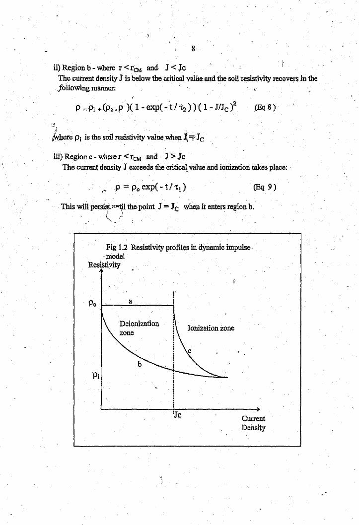
ii) Region b - where r < rCM and J < JcThe current density J is below the critical value and the soil resistivity recovers in thefollowing manner:
(Eq 8)
(Ikh,erePi is the soil resistivity value when 11/ '7 Jc
iii) Region c - where r < rCM and J > JcThe current density J exceeds the critical, value and ionization takes place:
p = Po exp(- t / td (Eq 9)
This will persisr'111t,ilthe point J = Jc when it enters region b.! \I
Fig 1.2 Resistivity profiles in dynamic impulsemodel
Resistivity
Po a
Pi
Deionization Ionization zone
CurrentDensity

9
The current impulse and the nonlinear resistance can be represented by an equivalent circuitshown in figure 1.3 below, The solution of this circuit is based on a time-iterative energybalance method which has been executed on a digital computer. Theresults compared verywell with experimental values [7J.
Fig 1.3 Equivalent circuit of surge generator andimpulse resistance
L Rs
c
TA similar model has been implemented recently 011 EMTP [13] with very good agreementbetween computed results and measured results.
Similarity approach - Korsuncev , Chisholm
A second model was originated by Korsuncev and extended by Chisholm.In 1958 Korsuncev applied similarity analysis to the surge respone of ionized soil aroundearth electrodes. He concluded that footing resistances of differing ground electrodesgeometries can be represented by two dimensionless parameters IIIand TI2 :
ITl == sREI P
TI2= p I/Ecs2
CEq 10)
(Eq 11)
s is -the characteristic distance from the center of the electrode to the outermost point.p is the oil resistivity.RE is the electrode resistance.I is the electrode currentBe is the critical breakdown field.

10
For each electrode geometry a value of illo is defined in terms of its low frequency lowcurrentresistance. n," values for typical electrode configurations lie ~'ithin the range of0.2 to 0.8, with hemisphere like electrodes having the lowest values and single rods havingthe highest values. ill° values can also be approximated in terms of the distance s and theelectrode surface area A [12].For example for a single rod and a hemisphere the following values of illO result:
TIlO(rod);::::0.4028 + (1I27t)x (In S2/A)
TI]°Olemisphere) = 0.4517 + (l/27t) x (In S2/A)
(Eq 12)
For Geometry dependent region (III:::: constant) ~ The characteristic distance s and thesurface area A are computed and equation (13) gives the ill° value. Equation (10) is thenused to compute the electrode resistance RE •
For Geometry independent regilln (ill = f (TI2) ) - Once ionized beyond the criticaldistance, all electrodes behave much like a hemisphere. Korsuncev has developed a criticalcurve n 1 :::: f (n2)~a least-squares fit to this curve in the range of 0.3 to 10 gives thefollowing power-law relation:
(Eq 14)
The power-law relation between the soil resistivity and the critical field is given by [12]:
E - '141 0.215C - k P leq 15)
The transition between low current and ionized respone occurs when IT1 value fromequation (14) becomes smaller than ITtThe combination of the two regions gives a complete model:For low currents an initial resistance is calculated from equations (13) and (10). For highercurrents equations (11) and (15) provide II2 value and the III value is calculated fromequation (14). As long as the TIl value is lower than the IllO value the ionization hasspread beyond the characteristic distance and the surge reduced resistance is calculatedfrom equation (10).
Comparison with results from the Liew and Darveniza model show that the initial lowcurrent resistances are lower in the Chisholm model and the surge reduced values fall morequickly 'with applied current. Both models converge to the same impulse resistance at highcurrents.

11
Experimental work in South Africa
Experimental work on practical earth electrodes, which included impulse tests of a ring-anda single rod, was done by Oettle and Geldenhuys [11]. The current flow into ohmicalyseparated sections of the electrodes was monitored.It was concluded by the authors that the model of a uniform ionization zone which is said. to surround the electrode whenever the critical electrical field is exceeded was notrepresentative of the physical processes involved under high voltage impulse conditions.However it was acknowledged that the mathematical model describing the phenomenawould be extremely cumbersome and not practical for engineering situations.The authors suggested that the uniform ionization zone model could be used as anempirical means of comparing the impulse impedance and the critical electrical field ofvarious electrodes in different soil conditions.
1.2.4 Extended electrodes - Dynamic models
Extended electrodes are beyond the scope of this project. However, for completeness ashort description of their behaviour modelling is given:
Two similar models have been proposed by Mazzetti and Veca [8] and Velazquez andMukhedkar [9] -A single horizontal buried conductor is modelled by a distributed parameter representationof the leakage conductance G, inductance L, capacitance C and resistance R - all per unitlength as illustrated in Figure 1.4 below:
Fig 1.4 Representation of ground electrode withuniformly distributed parameters
R,L R,L R,L--c::r--r---c:J~"----I

12
This representation is similar to a long transmission line. The only difference is that theresistance is negligible compared to the inductance, and the capacitance is negligiblecompared with the conductance.
The propagation of surge impulse currents into the soil can be considered to be governed bylaws typical to a conductive medium [8] [9]. Therefore, the wellknown equations ofpropagation may be integrated in order to obf?,)1nthe behaviour of the voltage and currentalong the electrode, as well as the impulse ifupedance.
The soil breakdown that occurs when a high impulse current is injected into the electrodehas been considered in the model as an apparent increase in the cross-section of theelectrode and therefore a decrease in ground resistance.
(I
~----.-------.--~~----'-------"~--

-'1
13
2. POWER FREQUENCY
2.L Experimental Set-up and Testing Procedure
2.1.1. Step potentials - field measurements
The tests were performed at the outdoor high voltage laboratory of the SABS NationalElectrical Test Facility (NETFA), Olifantsfontein .•A.:n HV Lab and test site plan is shownin Fig 2.1. Five different electrodes were installed at four locations in the open fieldadjacent to the HV Lab concrete floor. The distance between the nearest electrode (A&B)and the concrete floor was about 80m.A single phase 1.2MVA multi-tap transformer was used as an AC source. A single phase22kV line was built to supply the instaI!ed electrodes. This line was latter used for impulsetest measurements.
voltag~divider
0__.... impulse
generator E-!
Fig. 2.1 HV Lab and test site plan
A&B c
"room """outdoor HV lab (concrete floor)
A detailed soil resistivity survey of the field where the electrodes were installed wasperformed -results are shown in Appendix D. The various electrode configurations whichwere tested for step and touch potentials are illustrated in Fig 2.2. The dimensions are givenin Table 2.1.
Table 2.1 Electrodes dimensions
Dimensions A B C D Etrench length (m) 6 6 10 8 6depth (rn) 1 1 1 1 1r..:.dlength (m) 1.5 3 1.5 1.5 1.5no of rods 4 4 1 7 4

14
Fig. 2.2 Test set-up: Step potential and electrode resistance measurement
A&B c
* The star poinf'Gftlle electrodes Waslocated lrn away from the pole.{ 1 '
Test procedure
D
Each electrode was connected to.the supply line, one at a time, using an earth lead whichran up the associated wooden pole. The output voltage of the supply transformer waschosen as 250V because of earth fault protection considerations. Once the line wasenergised, the voltage on the surface of the earth was measured using the followingmethod:
A reference spike was driven into theground at a distance of about 25mfrom the point were the earth downlead entered the ground - at rightangles to the supply line. Then amultimeter was used to measure thevoltages between the various pointson the surface of the earth around theelectrode ( at intervals of 1m)
Fig 2.3. Step potential-method ofnl\l1
;i~
~ r!' .,
">(
.@
~__l___j

15
The voltage of the earth down lead and tIle c-etr{;.ntat the point of entry to the ground were _also measured in order tocalculate the apparent low frequency resistance of the electrode. "In a separate test the re31~~~tanceof the electrodes were measured using an earth resistancemegger,
\\~Observation: \It was observed that after a period or~ime.(about 40min) the current would \~!art to dropsignificantly, e.g. 42A to 32A.Thus if the current started to drop during the measurements, the test was then stopped for.a,while and resumed later atthe previous current level. I
This phenomena is attributed to the heat which is generated in the vicinity of the b~~dconductors (PR losses). The heat dries the soil and thus the electrode resistance increaseswhich results In a lower current.
2.1.2 EI(\ctrolyti~:o'f~lh~k-Step Potential
Th~!riteasuring circuit\',I'},I
The tests were performed at the Wits HV laboratory. Scale models of the various electrodeswere submerged in water inside an electrolytic tarl~:. The tank diameter was 3m and theheight was 1.2m.The tank was first lined with aluminium foil on the sides and the bottom and then filledwith water to a level of lm. The scale electrode was constructed using Nichrome wire ofO.173mm diameter (scaling factor of 57.8). Nichrome wire was selected because it):;;-mechanically more rigid and tends to oxidise less than copper. i;~-'_/The electrodeeas supporte. y a perspex structure and nylon strings.
A 230/24V transformer was used as a source ill series with a variable resistor. Anillustration of the circuit is 8ho\>Y11in Fig 2.4 below.
Fig. 2.4 Electrolytic tank test set-up
c-.__-~-----'--------~--~----------------~-~--~-~__}
-~-------~

16
Test procedure
The surface potentials around the electrode under test were measured using the followingmethod:
A square 3mx3m wood frame was fitted on top of the tank edge and measuring tapes wereattached to the top side of the wood on two parallel sides. - which was the Yvaxis. A 3mwood beam fitted with a plastic curtain rail and measuring tape was laid on top of the woodframe and a voltage probe was attached to a slider which was free to move along the curtainrail ..which is the x-axis,
The voltage probe was adjusted in such a manner so that its tip was 1em below .he watersurface. Fig 2.5 shows a top view of the measurement accessories.
Fig2.5. Measurement method
..... electrolytic tank.. " ,. .... - .. , ...... ~.,."
voltage probe and slider................... ~ .
Measurements were taken at intervals of 2Cll1.
2.2 Presentation of results
2.2.1 Field measurements
The results of surface voltage measurements of all the electrodes are presented in AppendixA in the form of equipotential lines.
The surface equipotential voltages of electrode B are plotted in Fig 2.6 on the next page.

17
Fig 2.6 Surface equipotentials for electrode B
I J I Ii nn tl\I . .' /..; _....... !' \-i-
Contours
minimum value 5Vmaximum value 80Vsteps of5V
I I 'II J i \ \\\ I / .--' ,-~~~++~~~**~~~7~~riH_, 1111)'//\ l/illl I
Bl
Electrode resistances
The apparent low frequency resistance of the test electrodes is shown in table 2.2 below
Table 2.2 : Apparent low frequency resistance oftest electrodesJ;_
Electrode Voltage (V) Current (A) R-=VII (n) Rmegger (0) f!
A 233 10.1 23.07 31.3B 203 41.8 4,85 -
230.8 -C 5.8 39.8 34D 226.5 9.5 23.8 23.1E 227 6.2 36.6 26.4

18
2.2.2 Electrolytic tank
f)
c.0
The results of the surface potentials of electrodes F and G are included in Appendix B.. ,
The surface equipotentials of electrode t are plotted in Fig 2.7 below
Fig 2.7 Surface Equipotentials for electrode F
~r !, ) ),), - ~.... ;_'" -::>i~"""" '''":'"",,,. r ~ i" \s- " .~r ,
// -> /. 'if \\-1\\ f'...", '..., "'-l~fW-I- 1\'/ { l ! if( (f ,"-,1\\\ -, " "1.- t-, .t-, \"
0 J, I itl '-) 1) i\ ~:'--.:';\. \ 1 \,
;:l I ( I / l if II .ll\ i, ", \ -, \. \\"- -4 I ( i ( f \', ,"I"",,-' I<~ 'i,
['..."" -, \ \I I ~'".) I I I J I ;1(; .'" \,\ '-", .>! ..' .... .."" .-,,'\ \,k 1 I ~ } (II~ .:;s; :::::::: ::::::-~~;'::;:: -::::....: Z\\ 'lJ.,:'-- ....
I \ hi II Jili \ , i\ " i \ \ II \ i\ \u I'i,l I
\11. 1rY I ) I I :1/ ' J 1
I ~ : \ \\\'\ r;::::::: -"/ .;:; -::: ~ ~ </ ILL U_f//
~ .\. : \ It \\£. /; _.....-I"""'--""-;' .-;-',/i// 'I~l \ I \ \ 1\ \ /1'/ /-"-,~ " '/ /~-~.\ ~\\\~\ \\ ('((V -->"/ r' . '('(I/ ( , I--;:1 \ \ ,\\1\11 ),) / i/ ,/ / / I-Itto \ 1\ \ \ \1\\ lY'/!J;/Y <. " ~/'I/I \ \ ,,-,'\\'\i\\ Z/ //.V.,., ",/ / /' " •/;:~fiIS \ \ ,\,r'~,~'~-;;;.:-/:/~.../ /' i / .', '7-h
\ ::;:[..L-';;I I I I ,Fl
2.3 Interpretation of results
Soil resistivity
.c'&.utours(Scaled up)minimum value 25Vmaximum value 125Vsteps 5V
Grid lines:Im x lrn(Scaled up)
Examination of the soil resistivity survey results suggests two featuresa. The soil resistivity at each location decreases with depth. The resistivity at a depth of
10m is 10 to 15% of the resistivity at the top layer.b. The soil resistivities at the various locations at the test field are ali in the same order of
magnitude of a few hundred Ohm at the top layer.

19
Electrode resistances
Examination of the different electrode resistances (table 2.2) indicates the following;a. There was a significant reduction in resistance when electrode A Was changed to
electrode B (using 3m rods instead of.l.Sm),This is attributed to the fact that the soil resistivity decreases with depth.
b. The electrode C resistance was the highest although it had the longest trench (10m).This could be attributed to the fact that it has got only one rod
c. The electrode D resistance was almost equal to the electrode A resistance although it hada longer trench (Sm) and 3 extra rods.This could be attributed to the fact that the soil resistivity around the electrode D locationare higher than that around electrode A.
d. The electrode E resistance was higher than D although the total trench length of both wasthe same (about 24m). This could be attributed to the fact that Electrode E has less rods(4) than electrode D (7) and the soil resistivity was slightly higher around E.
Scaling up of field measurements
The step potential tests were performed using a supply voltage of 250V. However,operating voltages on MV networks are llkV and 22kV with 6.3SkV and 12.7kV line toground voltages respectively.
Therefore the following scaling factors can be calculated:
6350SFIl = --- = 25.4
250
SF:20 = 12700 =50.8- 250
Scaling of the electrolytic tank measurement was done as follows:1. The actual electrode voltage, measured at the field, was divided by the respectiveelectrode voltage, measured at the tank.2. The tank electrode resistance was divided by the field electrode resistance.3. The earth soil resistivity at 2m depth was divided by the water resistivity (50.Qm).
The scaling factor was taken as: (l)x (3)1 (2)
The comparison of the results for two electrode configurations gives an error of 15%to 40% which is not acceptable. This shortcoming is probably because of the fixedelectrolytic (water) resistance in comparison to the soil resistivity in the field, whichdropped rapidly with depth.

20
2.4 Discussion
From the results for the electrode resistances it is clear that the addition of rodswith thesame length 10 the configuration does not reduce the resistance significantly. However.extension of existing rods where the resistivity of the soil decreases quickly with depth,results in dramatic decrease in the electrode resistance. This would probably not be truefor soils with constant resistivity, or where the resistivity increases with depth.
For electrode configurations which are more "symmetrical" (e.g. electrode E is moresymmetricalfhan electrode A ) ~ the maximum step potentials are lower. However, theimprovement is not significant. It is probably better to put effort into reducing theelectrode resistance in order to reduce the maximum electrode voltagr during a fault. Areduction in electrode voltage will inherently reduce the step potentials ~~oul1dit.
1\
Fig 2.8 below shows the electrode voltage and current as a function of its resistance.The values where calculated for a 22kV system with a fault level of 14M and a NeutralElectromagnetic Coupler, which limits the fault current to 300A. Two different linelengths from the source substation to the fault location, were taken into account lkrn and10k111.
There is a change in the voltage slope around the value of 40Q~below which the electrodevoltage drops rapidly when the resistance is decreased.
Fig 2.8 Earth electrode current and voltage vs electrode resistance
400-3001t:i
!;:o .-..
S. 200E ~t.:.. ........- 100a~
00
r-di~~rh.' . -===-:11" 2000 ...
: .: .. -:-.0 &
I lkm Mink Conductor I1--10km Mink Conductor I
"
--- J krn Min;~Conductor I~--- IOkm Mink ConductorJ
oN
o oeo c-o
Earth Electrode Resistance (Ohms)

2J
3 IMPULSE BEHAVIOUR
3.1 EXperimental set ....up and testing procedure
The measuring circuit
The tests were performed at the outdoor HV laboratory of NETF A. The test site pl~\,l1isshown in Fig 1.1. Tests were carried out only on electrodes A and B at the same location(see dimensions of table). Fig 3.1 illustrates the electrical test circuit. Fifteen of the impulsegenerator capacitors were utilised and connected in series.
Fig. 3.1 Test set-up: Impulse behaviour tests
i~···I~······;··················:::t·=Si:~:voltagedivider 2 v.- capacitor
banktailresistor
voltagedivider 1vI1
Impulsegenerator
.... ~ _ O' •••• '''' ~ o·
Two voltage dividers were used:- voltage divider 1: at the output of the impulse generator, using the HV laboratory earthmat as a reference.- voltage divider 2: at the electrode under test - the reference was achieved by drivingspikes at a distance of 25m away from the point where the electrode down lead enters theground - at right anglec to the supply line. These spikes were then connected to the LV sideof the voltage divider by means of a Mink conductor (llmm diameter).
A current transformer (Pearson coil AI) was used to measure the generator output current.A second current transformer (Pearson coil A2) was placed at the point of entry of the earthdown lead into the ground to measure the input current into the earth electrode under test.
In order to measure the current distribution in the ground electrode seven wide band currenttransformers were installed. These ""id,e band current transformers were of the Rogowskicoil type. The location of each coil is shown in figure 3.2.

22
Fig. 3.2 Location of Rogowski coils for current distribution measurement
Coils 1,2,3,4 were installed around the rods, just below the connection between the rod andthe conductor in the trench. Coils 5,6,7 were installed around the conductors in the trenchabout 40cm from the star point. Coil 8 was installed around the earth down lead.
Coaxial cable leads were, taken up vertically from the Rogowski coils to where they wereconnected to optical transducers. From there optical fibre cables were taken to the HV (J
measurement truck which was positioned 50m away. The physical distance between thegenerator output and the electrodes along the connecting line was 110m.
The voltage and current at the generator output were recorded on a Tektronics Scope usingseparate channels. The electrode voltage and currents were recorded at the HVmeasurement truck using the Nicollet facility which is a computer based data acquisitionsystem for high voltage transient measurements.
Test procedure
Electrode A was subjected to a series of impulses starting from a 30kV generator chargingvoltage up to I50kV. Voltage and currents were recorded at the points mentioned in theprevious section.
Once the electrode A tests were completed the 1.5m rods were pulled out and 3m rods wereinstalled instead ~this new configuration was named electrode B.

u
3.2 Presentation of results
3.2.1 Impulse waveforms
Typical voltage and current waveforms which were recorded are shewn below.
Fig 3.3 : Generator output waveforms
36.SkV/div
tim e: 20l1S I d iv
Fig 3.4 : Voltage and total current at the electrode
-I- 12.0KAmp KV~~--------------------------~---------------~i+1S0
}
+6.0
!I!1.90!
+0.0
.6.0
-12.0 :'1 SO
-20 +0 +20 +40 +60 +80 +100 +120 +140 +160 +180+200Time IlSeC

24
Fig 3.5: Impulse currents in coils #4 and #7KAmp
+6.0{)
+3,00
+0.00
-3.00
-6.00-20 +0 +20 +40 +60 +80 +100 +120 +140 +160 +180+200
Time p see
The \VaVefOlTI1S above were imported directly from the measurement instruments.Test waveforms for the variou~ voltage levels can be found inAppendix E.

25
.3.2.2 Current distribution
The distribution of currents in the electrode were calculated using the peak current values- of the waveforms on the legs of the three point star electrode (coil #4 and coil #7) as well asthe rod which was installed at the star point (coil #2).
The current in coil #7 was chosen as reference (100%), Then the current in the other coilswas measured and calculated as a percentage of the current in coil #7.There was some diversity in the results. The same exercise was done using powerfrequency. Fig 3.5 below shows the distribution of currents under low frequencyconditions.A summary of the results of electrode A is given in Table 3.1 below.
Table 3.1 : Distribution of current in the earth electrode
Type of Test Coil Current Coil #4 Current Coil #2 Current-l- #7 relative to #7 relative to #7
,
AC 100% 27%-33% 22%-33%-::--' .Impulse 100% 75%-90% 95%-130%- -
Fig 3,6 Distribution of power frequency current electrode A
Amp v!+600
+0.0
-12.0 "j,300, \\ II
\ / 1\ I i\j I
,_ --- --_~_-_1·600
'{ .: J, j \ " C '17i·J 01\.\./
\
\f{ IJ\ / Coil't
.24.010.0 10.0 20.0 30.0 40.0 50.0
Timems

26
3.3 Interpretation of results
3.3.1 Reduction in electrode resistance
Fig 3.7 Electrode Resistance vs Peak Current
18·
...... 16'"E 14..t:0,_, 12C1)us:: 10(tS
t;;.c;;8..,
~C1) 6·'"0eu 4..,i.ll 2
00
A
2000 4000 6000 8000 10000 12000Peak Current (Amps)
Figure 3.7 above demonstrates the reduction in the conventional electrode impedance.the curve for electrode A gives a reduction factor (from its power frequency low currentvalue) of 3' to 3.5 at currents. with a peak greater than 8kA. However the electrode Breduction factor is only unity. This could be attributed to drying of the soil around theelectrode during tests. It was also noticed during step potential measurements on thiselectrode configuration that the apparent resistance was increasing with time and the testhad to be stopped for a while.
The slope of the curve for electrode A is much steeper than that for electrode B - this agreeswith previous studies where it was normally found that where the low frequency lowcurrentimpedance is high the fall to a reduced value is faster (7] [12].
From Figures 3.3 and 3.4 it is noted that the front of the voltage wave form as measured atthe output of the generator is much steeper than at the electrode ~This is the effect of thelong loop inductance. The peak voltage drop (20% to 25%) is also attributed to the longdistance that that surge has to travel.The current peak at the electrode occurs after the voltage peak. There is a time delay ofabout 50 111S.Both currents, which were measured with separate and different instruments, at theelectrode and at the generator have the same peak magnitude. Therefore the results could betaken as correct with relatively high confidence.

27
3.3~1Current Distributioni \
The difference between the #7 and #4 currents is the current which dissipates from theconductor in the trench. The lengths and current distribution at low frequency is given intable 3.2 below. It appears that the currents dissipating from the conductor in the trenchand from the rod are proportional to their length.
Table 3.2 Power frequency current - proportional distribution
length (m) dissipated current (%)conductor in trench 5.5 (80%) 70% .,rod 1.3 (20%) 30%total 6.8 (100%) 100%
However under impulse conditions most of the current (75p90%) is being dissipated fromthe rods. Furthermore, rod #2 is dissipating more current than rod #4. TIns could beattributed to the fact that rod #2 is closer to the point of current injection.
"In Fig 3.6 there are phase shifts between the various currents, while one would expect tohave them all in phase because the electrode is treated as a resistance. These phase shiftscould be attributed to the integrators in the Rogowski coils.
3.4 Discussion
In general the results which were obtained from the impulse tests agree with previouspublished work. [7] [11][12] - there is a reduction of electrode impedance under impulseconditions. The current peak occurs after the voltage peak - this can be attributed to theionization time constant (7] [10] [11].
The more interesting observation from this work. is the different current distributionbetween the electrode components under impulse conditions. It appears that heavyionization is taking place around the rods rather than around the trench conductors. TIle soilresistivity around the rods is lower by a factor of 2 to 3 compared with around the trenchconductors. Lower soil resistivity implies that for ionization to take place a higher currentdensity is needed. The nonuniform electric field near the tip of the rods may also contributeslightly to the increased ionization.

284 CONCLUSIONS AND RECOMMENDATIONS
4.1 Conclusions
1. Where soil resistivity decreases with depth, use of extended rods in the electrodeconfiguration results in significant decreases in electrode resistance.
2. Changing the configuration of an electrode to a more symmetrical shape does have aneffect on the maximum step potential. However this effect is not significant.
3. f{esults of scale model tests in an electrolytic tank did not agree well with the fieldmeasurements. It is concluded that the problem is that the water in the tank ishomogenous, whereas the soil resistivity in the field decreased rapidly with depth.
4 ..Reduction factors (from the initial low frequency low current electrode impedance to thevalue under impulse conditions) of 3 to 3.5 were recorded.
5. The current distribution between the electrode components is different for power ..frequency and for impulse conditions. For power frequency conditions the distribution ofcurrents is proportional to the length of the conductor or rod. However for impulseconditions most of the current is dissipated from the rods due to higher ionization. Thisstatement is true for soils with decreasing resistivity with depth.
4.2 Recommendations for further work
. Power frequency
It is recommended that a computer modelling be used to try to reconstruct the resultsobtained from the full scale model. Such a simulation could then be used to optimiseelectrode configuration design
Impulse behaviour
Impulse tests on electrodes buried in a soil with constant resistivity and tests on electrodeswith no rods at all would probably provide a more complete understanding of theirbehaviour.

APPENDIX A. - :tULD f\.mASUREMENTS RESULTS
Fig Al : surface eq~pmenti,als for electrode A
Al
~. / 11 \ \ ,\ \ \ 1 '\lAY i~" \1\ .........
({
v Jr,~
\
! <,~.
r-,.~ t---.~'!f!
r..(9 r;..:::: 'IIwz ~ '/
, 1\ 'I I.YI I \ .; \..... i-- V,Vir#. 111/ v ..........r=flrl! / ( .I
lVi '/ / v......- J / _/-, ~ /'
Al
trench depth 1mradiallength 6rurod length 1.5m
number or rods '"
"'V""233V*la 10.2A:.R =< 23.0f.'l'" lueasured at the point where the earthlead. enteJ'll ~ ground
NRntegger :::.::31.30** ~ using an earth resis¢ance megger(DETS)
tninim1!lll1 value 5Vmaximum value 70VstepSofSV
Imx Im

Fig B 1 : surface equipotentials for ~IectrodeB
Bl
t .- -....,
/ :,. i'\.l~ / / -- I\.... '-""- 11
V /'_- z- 1\p- / It: :;:;:: ~ ::s;~ "\. 1
II. \\ \. <;
~ I 1\ \ \ "\.~ :1 \ ...... ~.... "'J Il . "-~ II! '" \ I /;(. j t:~ :'..~. f ... '" :s; \t '\ .."'-u ~ '1111 J/
\ ~ B~I I--- r.- I I 1\
fr v t-"
.. III I ~ /
'"! III 1111 If! il / /'
Y ss V- ,/ 7_,
! <, \I\:~ r;:;::; /' 7 I~ '\. r:;; IY rl
:i~..... I\_ ._ r: ~
'\. !-" 1/ VI-.. -I-'" v
~IO.J'<t""'lOl~ :o::liz~ ) c
81
Cofigumtion:
trench depth 1mradialiength 6mrod length 3m
ntunbeiorrods 4
·V=203V...I=41.8A.·.R==4.85.Q... ~ at the point 'Where the earth
lcadenteB the ~
mininl1un value 5Vma.uum value SOVstepsofSV
tm x Im

FigC I : surface equipotent'ials fur electrode C
Cl
t,v f.-
f ~
1,\,K ~\ .\ \I---" I ?I \
If,\ I. \.'/ ,\ ....A~II " ...!ln ....... I--
~ / I)) J 1'-h f'.... r-,~ IJ Uri/. rA' ., 1"",! \
~""IS l\
'! I ~ ~tiF::: :;;: f- rJ 1/,\\l\\ LV'l- r/.~ ::.- [/\.~I\\ IV 'I fl ,..1-- !-- i-' V. II \I 'f v I-l\ 1\ " IfII II 1\' f
~ n ~VI, I Ift. I-.... \ II 'I<:t 1/ LI: tV II
1\ tv. r; It If
=i; 1\ '-I:;:'8r-, t-'
6 :, '0 [t[2.0 I U J "t ',;) .t:. • ) 3 J I) J
Cl
~---------------~D' .~
trench depth 1mradiallength 10mrod length !.Sm
number or rods 1
*V=230.SV*I=5.8Ar,R=39.SO...measured at the point where tbe earthlead enters the ground
",. Rmegger = 340+.measured using an earth resi~1a1'lcemcgger(DETS)
Contours
Minimum value 10Vmaximum value lOOVstepsoflOV
Im x Im

Fig D1 : Surface equipotentials for electrode D
Dl
ft,~
-" ~r'- <,r ....... ~ "..... "-V;~ ,\, , i\
III rA~ ,\. ...... (( III 1\ '\ "\ :--.~! t ( [" \\ t\ 17.... In r-...
11 1/ rv r-, r-.~ III 1\ , N- l- I- ....... r-. I'" '\
IIr- ~ ~ ~ " "'\f- \\ II ,
~ wm I~ I/":~ \11 In If/ 'r' r....... I-- I--' J
1\ II r\ '/ v ~1\ I l\' IV, 1/ I( V r: 1/I \ n II ' I II I _. I-.~ 1\ \\ fYlr/J t
t: II ,\ ~ II II;;'f \ "t:"- r---:...- I~ 1/.~ ,<, ./"!~!:
'",',..".'", ",: .. -") j '0 '11[2""UJOY",,u.l, .
'\(
Dl
Configuration:
-.., •
dimensiQns
trench depth Imradiallen,gtb. smtodIengili 1.5m
number or rods 7
*V=2'1.6.5V.. I :=;9.SA.·.R""'23.S0.. 'I1lCt\5Ufed at ~!POint ".there the ~rt11
lead enters the ground.
.*Rmegger = 23.1.0*.measured using an earth resistance megget(PETS)
Contours
ntini.tnum value lOYma.-dnnnn value tlOVsteps of lOV
Im x lm
A4
•

Fi8 El : Surface equipotential for electrode E
El
~
'I
1,l;h1",:!.. I--f.!. .r: h. i0'- ...I.!~ r '/ '"II! /'/ ,_.... :.-.- f-- -- ..... r-,o? I '/ ~ ~ t-- :--. r- "'t if j II I flf rr....:18 ~ t:.-.: t"- t-- ..... \~ 1/ ~ t.:: ~~ lliIlIIlll\ ill. IS:S ss !:.':: ;:-..
tr 1\\ 1"\.' '" l\ .\ "'1J .c ~ rl '/ fl-I JI P::~ ~ ~P::~ 1\ :/ V.~ ,l \ 1\ ,\ l't::;: r.::;:;~ t;::- c- :.-- /'! \ l'\ ~P:: r..- 1/ /' /~ I\I't"- I......- - l/
*Y- I' r-, l- I--'!_ I" -I---'u i'--
1~lr I- r'l,l;
El
Configuration:
Dimensions
trench~ Imrndia11ength 6mrod length 1.5m
n~ror~ 4·V=224V*I=6.2A:.R=36.60
...~ at the point where the earth teadentel'S the ground
,..'"Rmegger == 26.40•• measured using an earth resistance megget(nETS)
minimum value IOVmaximum value 180VstepsoflOV
lin x Im

APPENDIX B - ELECTROLYTIC TANKRESVLTS
Fig Fl : Surface equipotentinls. of electrode F
Fl
:7 / II Li,l'::>' ;i,;:~ :--.;: '-, <, "- } "-.,\0 I V/I/, 'I) "" \.\ i'...' c"""C'-K'---~[\F ( II f if I ( 'r ."'-'~\ ~. ,," '- ........ r-, 1'-.1'\u / / I 'f "7 II 1,\ i', I\~" \., 1II v ( I{ f I t "- I, \ '\" -, '\ " \.1\"f' ( rtf\.. .'\."- r-: .......__, --, ......... "'-' ."\ \1.:J rt. <,~\ <, ....... 1'--' ......... .-, c'\"" ::--= ~ t:.:::- .:::::R :=:::: ~ \\\.l _\ \ \ 1\ \ \V' I I.. ~U) f ) II I I.~It --= ~ ~ :% IJI_., -- ::..-"" \ l\\\ ~ vI /" / ......... v.......--:. ::/. ,/ '/~ \ \\/ '//V ./"I/'.: / V /1/"t' \ \\ r\ ~ , \ \ \ ( (/" .... '/ / / r rf_,
\ \ \ \ ,\\ ) j} / ,/ v / V /u \ 1\ \ ,,\ '/ fj; .: // v/ /' V //. \,\ "\.'\ \: '/./ V/- /_.; ./ ,/ /;; r~ /./0 '\ \ "'~ ~~ V '/ -: /' ~ /'/:iF
-5 -4 -g --Z -1 0 1 2 3 4 5 6 1 8 9
Fl
Configlltation:
~ •.
trench depth Imradial length 6mrodlcngth 3m
nunmetotnxm 4
*V:= 18.92V1=101.SmA
...R=186.4Q" measured at the point where 1he wireentered the watel'
Scaling:fuctor == 15.4*418.08=1.4
Contours
tmnimum value 2SVmaximum value 12SVstepsofSV
Imxlm(scatedup)
B!

Fig 01 :Surface equipotentiais of electrode G
Gl
o / f/ /-:;....-.." .....__".........'-<:n, 1 J f .........'\\,"'- "'- ~ "" ( A'-''' " " ........., '-..., ""',;;J ............."-,~,'--.......... " ',,-- "
'\' ( r~i''-'"-;;;::::"''' ,,, .., t (r-...:---.:::::--:: ........:--..... "-"",,~ ~~~~~~~~~.l 1/ ......,.~ .......~ t\.:: "'-.. 1'---1'-{1 [\ r--!7V%V/:vC::.l 0~~~~~-~~'" \ u-""'v/:v/'" v V /.;;, ( \..vv/ ./ _...v V ......"t /,,:/~7 V/' _.,v /v;;J 1 I V/VV /' __...//v _/v0\ t\/i/IV/ V·V
~~~~~~~~~0123456701
Cofiguration:
B2
Dimensions (scaled up)
trench depth 1mradia11ength 6mlod length 105m
numwcrornKh 4
"'V=15.1SV1= 103.1mA
:.R= 146!l.. tneamJred at \lhe pmnt where the wire
entered the water.
Scaling factor=lS*S/4=18.15
minimum value 70Vmammwn vatue210VstepsofSV
~
Imx lm(scatedup)

APPENDIX C - TEST EQUIPMENT Cl
ROGOWSKI COILS
A Rogowski coil is an air-cored current transformer with the main current c~tYng~~::~conductor acting as the primary winding. The secondary winding is terminated in a passiveresistor-capacitor (Re) integrator, as shown in the figure Cl below:
Fig Cl: Rogowski coil ~ Circuit diagram
r···········~···_···_·N ..••..• ~. .1 Passive integrator
Ri~~----+---rVx i ---L- Ci
IVo
TJ ~~.----------~-----T----~O
•• - •• - ••• -- ••• - •••••• ~- ••• _ •• _I
Vx == M* dl/dtM
Vo = ..---------* IRi*Ci
The advantage of using an air core is that very high currents may be measured withoutsaturation and bandwidth problems. The limit of the system's bandwidth is determined bythe RC time constant of the integrator. The period of the lowest frequency signal should bevery much less than the product RC.For the Rogowski coil used in the tests, the.RC time constant was approximately3 milliseconds ~resulting in a low frequency cut-off of about 320 Hertz. A standard8/20 microseconds current impulse is well within the required limits.
For low frequency steady-state measurements, the transfer function is determined by themutual inductance \....zl) and the rate of change of primary current (dl/dt), For 50 Hertzsinusoidal current the transfer function is given by:
Vol 1= 2*rr*50*M

APPENDIX D - SOIL RESISTlVlTY MEASUREMENTS

1,<¥kRkXXXXX~'O<XXXXXXXX><XXX x xx>sx><?~Xxxxxxxx x:< x:xx X':X~X>:;xxx><xxxxXxxgx:xxx X Y. ':,j,:.: ...:;.~x xx xxx xx Xxxxx xwJi LOCATIONS OF SURVEY'S AT NETFAWI-<t:t!)
GIJ-19 Oh"",netcrs 9
E LE C. 'p/ r/f?/
46]-1" Oh,,-~.trr. 3~
>(
x
327-3~ 0\1"
235-2" Ohlll"'liders»;
8./-,xX-Xy.X
303-29!lIl.-~.l'r5 4
"
!Xx:Xxx.:'(
"':
.tJ~-.c4 Oh.·"r.ters' 10
EL~C. 'c'
51G-30 (Jtco- •• hr"
718-35 O!l.-.tt .. ~
327-41 O",,· •• l er-s
65 ...... 5 cnfl"fIleLer5
ELl;'c...'O 1
2
901-72Oh~·•• t.rs 5
x."<i(
."x.~x.<xx):r.~-:x.xX.,<XXvx.xx;<.
x.,..~"(
,xxx
xxxxxyXx'>(
x,:v:x)(
xxxx.X,l<XX
t:IlaO
c

D2
150100
50
O~--~--~~~--~--~~\~----~--~--~--~o 2 4 6 8 10 \\12 14
Interval "a71 (M(\eters)16 i8 20
Wenner Survey 2'Resistivity(Ohm-meters)350!------~-----------------------------
300~ .....\, \
250 .. , - \
200 r \\i50 r "-.., .100r .. . ~ .. :- ••.•...
5~ [ . ~"",:',;",__:_'..:..' ~'..;_'........;.....;~-
o 2 4 6 8 10 12 14Interval "a" (Meters)
Wenner Survey 3
16 18 20
Resistiv ity( Ohm-meters)500~----~----------------------------------~
300
2 4 o 8 10 12 14Interval "an (Meters)
16 i8 20
400
I'

NETFA SOIL SURVEYWenner Sur'{ey 4
D3
Resistivi1y(Ohm-meters)S50~-----------------------------------------------.300250200150
'00
50oL---~ __~ ~~~~-- __L- ~ ~~~ ~~
o
. -\\
2 4 6 8 10 12 14
Interval "a" (Meters)16 18 20
Wenner StJ[\t§Y 5
1:;;I"Si';~:=__..__~:•...~~.~ ._.._.4ooLI\. . . . . .....- ..~ --... ; ... -.
20: .-_ ·i; - ---._ -- -"~ I
o 2 4 6 8 .'..1..1 12 14 i6
Interval "ali (Meters)18 20
.Wenner Survey 6Resistiv ity( Ohm-meters)
600r----600400SOD
200
......\\."~ ....-'.-.---.100 _,--O~--~·- -L __~. L-~~~ __ ~ __ ~I ~I~ __ ~~
o 2 4 6 8 10 12 14 16 18 20-
Interval "a" (Meters)
Oepth=3/4x"a"

:~~ ["SIStiv\ity( Ohm-me ters)
:~~r \~~~t -- ;\~r---l...---'--__'_---'----'---_'__---'-_--.J
a 2' /i 4 6 8 10 12 14.. /
If. Intervalta" (Meters)
!Iil
NETFA SOIL SURVEY.: Vvenner Survey 7
16 18 20
Wenner Survey 8 .Resls tivity( Ohm-meters)250~-~--~---------------------------------'~~
100
\\\\. II
'\~!J/.'5: ~_..l..-...._-!...-_......l.- __ --,- __ .-_-...J....- .... _. "--'-~--'-_~____' __ .l.-_J
a
200 .-..
'150 - .. -_.-
2 4 6 Bff 10 12 14
Interval "an (~ters)16 2018
Wenner Survey 9Resis tivi ty( Ohrn-rneter s)700~--------~----------------------'~---~
600500 .--...-~...400300200100 .. ... ..
a0 2
~ .•. "'.'''-'' .._ .._." ---..-- . . ' -." -'1
4 6 8 10 12 14
Interval "a" (Meters)16 18
Depth=3/4x"a"

NETFA SOIL SURVEYWenner Survey iO
Resis tivlt y(O hm-rne ters)
500 l I)
400 :/ '<,, """",
300 ,
::tt.........". ......-----''-'-_,.~-._._.'_"-,_'.----.-._:..- __"-""""_'o 2 6 a 10 12 14
Interval "a" (Meters)18164
Wenner Survey ii
400
200
2 4 18 206 8 10 12 ,4 '16
Interval "a" (Meters)
Depth=3/4x·a"
DS
20

APPENDIX E - IMPULSE TESTS RESULTS
E!ectrode 'A' test
Charging voltage: 30 kVGenerator Output:
1QK5tOPj:!Qd: 20StStSAcqUlcltlOrs
~ent;O.4
~
R1
M 101J).lS 1 .r . 0 1/
Ref2 "COrnV ~O,OMS
At the electrode:KAmc . KV
+00
+O.!3Q +120
-0.00
_._- .........._-- ..........--1
.0.00
-1.20
·20 +0 +20 +40 +60 .00 +100 +120 +101() +160 +180+200"Ome uSee

'11
Charging voltage: SOkVGenerator output:
""R;lK StOpj::lQdl <!(l1I6G At;quil:ttlol'$.... I [r-----r J i j
M 1OO~S , J' 0 V
Ref4 1.00 V 20.0/1.1&
At the electrode:+6.00
+3.00
Channel 9.:voltage------~------~----~--------j+0.00
-3.00--Ohannel S;lmrrent
EZ
R4 : Voltage 18.3 kV / div
R3 : Current 0.4 kA / div
KV+160
+80
+0
-eo
-20 vO '1'20 +40 +60 +11(1 +100 04120 +140 +1(;0 +180+-200TIm&IJSec

Charging voltage: 7SkVGenerator output:
\1
"RlI< Stopf!lCld: 211B56Acqull:itiors
M ',cc}J.s' eFt1 J C V
Ref.2 2.00V 20.0~S
At the electrode;
+12.0
+6,0
voltage
+0.0
R2: Voltage 36.5 kV / div
R3 : Current l.:izA / div':)
+130
,--.....u...L.c_I~·Current·6.0
+0
-13J
~w ~-20 +0 +20 +40 .:1'60 -eo +100 +120 +140 +160 +1W200
Time usee
\~
E3
(,

E4Charging voltage: lOOkVGenerator output:
~ stoppSd: 2'nH~~.Acqull:ltlons
R4: Voltage 36.5 kV / div
R3 : Current 2 kA I div
Ref4 a.eo V :;!O.OtJ.G
At the electrode:
+12.0KAm
+180
+6.0
+0.0 +0
-6.0
current
~w ~-20 +0 +20 +40 +00 +60 +'100 +120 +140 +160 +18Ot~
TIme IJSec

jl E5Charging voltage: 125 kVGenerator output:
~ stopPGc.!: 21O'1lilSISAcqulI,ltlOns
R2 : Voltage 91.3 kV I div
Rl : Current 2 kA I div
Ref::! s.eo v 20.0tJs
At the electrode;KArnp
+36.0
+24.0
+12.0
+0.0
KV
voltage
+280
+140
+0
~w ~.20 +0 +20 +40 +lta +80 +100 .,120 +140 +160 +180+200
il Time usee

Charging voltage': 150kVGenerator output:
'TI:r.'K St:O~:9d: ,2Q(iriS,A~O~ 1I
At the electrode:rKA~m~ . ~ ~.v+12.0 . '""1+280
+6.0
voltage
+140
+0.0
-6.0 ·140
--12.0 .......+-- -280.Z(J +0 +20 +40 +60 +80 +100 +120 +140 +160 +180+200
Time usee
E6
R4: Voltage 91.3 kV I div
R3 : Current 2 kA I div
+0

E7Electrode 'B' tests
Charging voltage: 30 kVGenerator output:
"Tel< 5toppl2d: 2ga5!5 A~UIs:jtiol"G
R.4 : Voltage 9.1 kV I div
R3 : Current 1 kA I div
Ref4 500rnV 20.0MB
At the electrode:
+160
+80
+0
-80
~20 +0 +40 +00 +80 +100 +120 +140 +160 +'180+200Time IJS

, )1
E8Charging voltage: 50 kVGenerator output:
At the electrode:KV KAm
+1:, .
current
"
J-._......;'-----.-_....-_..,...,..._..-----. _ __,.---.--_-..---r12-20 +0 +20 +40 +60 +60' +100 +120 +140 +160 +180+200

E9Charging voltage: 7SkVGenerator output:
~Stopp9d: "ggur; A~UIs:ItIOns
R4: V.pltage 36.S kV i div
R3 : Current 2 kA I div
Ref4 20.0}l1l
!'wi 100).tS i r 100mv
2.0DV
+280
. At the electrode:
+140
+0
·140
voltage
+6.0
+0.0
current
-6.0
.__.--T-....,....-~--...---.----.--.....-~~....--._--r 2.0·20 +0 +20 +«1 +00 +80 +100 +120 +140 +160 +t80+2OO
TIme Il3

El0'charging voltage: 100 kVGenerator output:
\)
(
~ Stopped: ~g1366 AcqUisitions
R2 : Voltage 36.5 kV I div
Rl : Current 2 kA I div
2.00V 20.0,IJ.s
At the electrode~~~ ~ .~ __ ~~KA~~
+280 .1 ~ • +32.0
+140
voltage
+16.0
+0 +0.0
-140 -16.0
-280. -20 +0 +20 +40 +00 +60 +100 +120 +140 +100 +180+200
TIme IJS
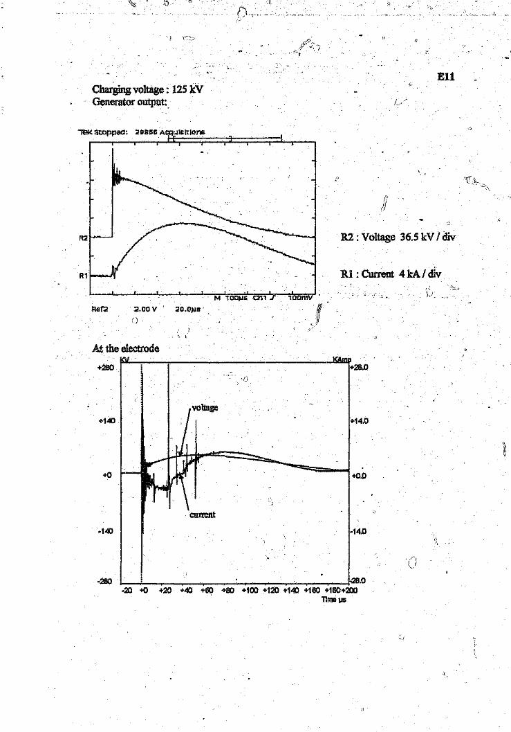
EllCharging voltage : 125 kVGenerator output:
~Stop~oc:: 21)8155At;qt.lil:ltiCns
R2: Voltage 36.5 kV / div
1.r 1oon1V
2.00V 20.0","s
'. I
At the electrode
+0
->14.0
+28.0
+140
+0.0
current.140 -14.0
-280 28.0-20 +0 +20 +40 +60 +80 +100 +120 +140 +160 +180·~200
Tlme !.IS
'.;_'
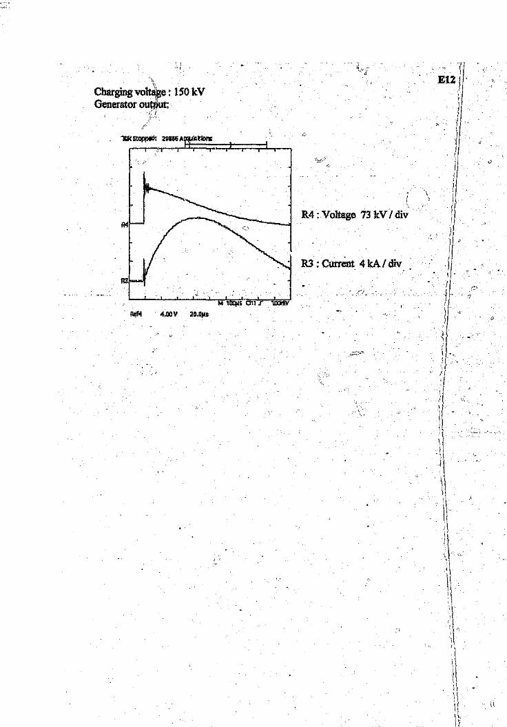
Charging volta~e : 150 kVGenerator outsut:
'/ i
( I :, • I· t
Ref'! 4.00 V 20.0),s
R4: Voltage 73 leV/ div
R3 : Current 4 kA I dlv
\1

REFERENCES R1
1. IEEE Guide for Safety in AC Substation Grounding. ANSIIIEEE std 80~1986.
2. Substation Grounding Scale Model Tests. EPRI project 1494-3 Interim report May 1983.
3. Caldecott R. and Kasten D.G., Scale Model Studies of Station Grounding Grids, IEEETrans. Vol. PAS~102, No.3, 1983.
4. Thapar B. and Puri K.K. , Mesh Potentials in High-Voltage Grounding Grids, IEEETrans. Vol. PAS~86, No.2, 1967.
5. Blattner C.J. , Prediction of soil resistivity and Ground Rods Resistance for Deep GroundElectrodes, IEEE Trans. Vol. PAS-99, No.5, 1980.
6. Takahashi T. and Kawase T. , Calculation of Earth Resistances for deep Driven Rods inMulti-layer Earth Structure, IEEE Trans. on Power Delivery, \'016, No.2, 1991.
7. Liew A.C. and Darveniza M. .Dynamic Model ofImpulse Characteristic ofConcentrated Earths; IEE Proc. V01121, No.2, 1974.
8.Mazzetti C. and Veca G.M. , Impulse Behaviour of Ground Electrodes, IEEE Trans. VolPAS~102, No.9, 1983.
9. Velazquez R. and Mukhedkar D. , Analytical Modelling of Grounding ElectrodesTransientBehaviour, IEEE Trans. Vol PAS-I03} No.6, 1984.
10. Oettle E.E. , The Characteristics of Electrical Breakdown and Ionization Processesin Soil, SAIEE Trans. 198.8.
11. Oettle E.E. and Geldenhuys H.J. , Results of Impulse Tests on Practical Electrodes atthe High Voltage Laboratory of the National Electrical Engineering Research Institute,SATEE Trans. 1988.
12. Chisholm W.A. and Janischewskyj W. , Lightning Surge Respone of GroundElectrodes, IEEE Trans. oJ.!Power Delivery, Vol 4, No.2, 1989.
13. Cattaneo S. et AI, Transient Behaviour of Grounding Systems Simulation: Remarks onEMIP and special codes used. EMTP Trans 199,3.
14. Meliopoulos Salas A.P. , Power System Grounding and Transients, Marcel Dekker Inc.1988.
15. Analysis Techniques for Substation Grounding Systems, EPR! final report EL~2682,Vol 1 and 2, 1982.

R2
16. DawaIibi F. and Mukhedkar D. ,Optimum Design of Substation Grounding ill TwoLayer Earth Structure, IEEE Trans Vol PAS-94, No.2, 1975. '
17. Bellashi P.L. .Jmpulse and 6O-Cycle Characteristics of Driven Grounds, Trans AlEE,Vol 60, 1941.
18. Bellashi P.L. Armington R.E. and Snowden A.E.~Impulse and 60-Cycle Characteristicsof Driven Grounds, Trans AlEE, Vo161, 1942.
19. Petropoulos G.M. , The High Voltage Characteristics of Earth Resistances, J. lEE, Vol95 part II, 1948. '
II


Author: Eytani Dan Mordechai.Name of thesis: Earthing electrodes- power frequency and impulse behaviour.
PUBLISHER:University of the Witwatersrand, Johannesburg©2015
LEGALNOTICES:
Copyright Notice: All materials on the Un ive rs ity of th e Witwa te rs ra nd, J0 han nesb u rg Li b ra ry websiteare protected by South African copyright law and may not be distributed, transmitted, displayed or otherwise publishedin any format, without the prior written permission of the copyright owner.
Disclaimer and Terms of Use: Provided that you maintain all copyright and other notices contained therein, youmay download material (one machine readable copy and one print copy per page)for your personal and/oreducational non-commercial use only.
The University of the Witwatersrand, Johannesburg, is not responsible for any errors or omissions and excludes anyand all liability for any errors in or omissions from the information on the Library website.