Impulse-Response function

Analysis: An application to

macroeconomy data of China

Author: Cao Lu & Zhou Xin

Supervisor: Changli He

Date: June, 2010

D-level Essay in Statistics

Department of Economics and Society, Högskolan Dalarna, Sweden

1

Impulse-Response function Analysis: An application

to macroeconomic data of China Author: Cao Lu & Zhou Xin

Supervisor: Changli He

School of Economics and Social Sciences, Hoskolan Dalarna,

D-Level Essay in Statistics for M.S. Degree

June 2010

Abstract

In this thesis, we make a comprehensive view of economic development, and choose

four typical indicators to analysis China's macroeconomy. The four variables is gross

domestic product (GDP), Consumer Price Index (CPI), money supply (M2) and

seven-day interbank rate. This thesis uses vector auto regression (VAR) to model

these four economic indicators from 1996 to 2008. And we do Granger causality test

to determine the Granger-cause between variables. Then we explain the relationship

among these four factors with impulse response function (IRF), which give an

overview of China's macroeconomic system. According to economic theory and the

results of impulse response function, there are complicated and significant

relationships among these four variables. At last, we make a forecast to China’s

macroeconomic in 2009, and compare the forecast value with real value to evaluate

the forecast effect of this model.

Key words: impulse response function (IRF), macroeconomic of China, vector auto

regression (VAR), Granger causality test.

2

Contents

1.Introduction: ..................................................................................... 1

2. Data ................................................................................................. 2

2.1 The Source of data .............................................................. 2

2.2 Description of data .............................................................. 3

3. Modeling.......................................................................................... 4

3.1 Vector autoregression ......................................................... 4

3.2 Transformation of data ..................................................... 5

3.3 VAR Lag Order Selection ................................................... 6

3.4 Models selection .............................................................. 7

3.5 Estimation for the model .................................................. 8

4. Impulse response function ................................................................ 9

4.1 Impulse response function................................................... 9

4.2 Empirical analysis: ............................................................. 10

5. Testing procedures ......................................................................... 12

5.1 Granger causality test ........................................................ 12

5.2 Testing analysis.................................................................. 12

6. Forecast ......................................................................................... 14

7. Conclusions .................................................................................... 17

Reference .......................................................................................... 19

Appendix: R codes .............................................................................. 19

1

1. Introduction:

Macroeconomy deals with the performance, structure, behavior and decision-making

of the entire economy, which can be a national, regional, or the global economy.

Because the macroeconomic includes many sophisticated relationships, only one

variable is hard to represent how the whole economy functions. In this thesis, we

make a comprehensive view of economic development, and choose four aggregated

indicators to analysis China's macroeconomy. The four variables are gross domestic

product (GDP), Consumer Price Index (CPI), money supply and seven-day interbank

rate.

To build the model for these four variables, we use the method of vector auto

regression (VAR). VAR is an econometric model used to capture the evolution and the

interdependencies between multiple time series, generalizing the univariate AR

models.

This thesis focuses on the China’s macroeconomic system. It uses four important

economic indicators, which are the monthly data from 1996 to 2009, to represent

the China’s macroeconomic system. The aim of this thesis is to model and forecast

those economic indicators with VAR models, explain the relationship among these

four factors, and give an overview of China's macroeconomic system.

Chapter 2 of this essay describes the specifications of the data we got and how to

transform the data, and then present a descriptive statistical analysis of these four

variables; chapter 3 builds vector autoregression (VAR) models; chapter 4 explains

the relationship between these four factors with impulse response function (IRF);

Chapter 5 considers Granger causality test to the models; Chapter 6 forecasts

2

[1] The gross domestic product (GDP) is a measure of a country's overall economic output. [2] The consumer price index (CPI) is a measure estimating the average price of consumer goods and services purchased by households . [3] Money supply is the total amount of money available in an economy at a particular point in time. M2:

represents money and "close substi tutes" for money. [4] seven-days interbank rate refers to the short-term funds lending rate among banks in seven days.

macroeconomy of China in 2009, and compares the forecast value with real value to

evaluate the forecast effect of this model; Chapter 7 uses the results we get in

previous chapter to explain the relationship between those factors and the forecast.

2. Data

2.1 The Source of data

The data we employed in this thesis are monthly observation of china’s gross

domestic product [1], consumer price index [2], Money supply (M2) [3], seven-days

interbank rate[4].

The source of Quarterly GDP is China Statistical Yearbook. Monthly CPI is from

National Bureau of Statistics in China. Monthly money supply is from People's Bank

of China. The average monthly seven-day interbank rate is from People's Bank of

China.

According to the data we collect and the request of model, we decide to use monthly

data of the four variables from 1996 to 2009 to build model. Because we can just find

quarterly and yearly data of GDP in China, we have to create artificial monthly data in

some way. Below is the process of creating artificial monthly data.

For GDP, the original data we got is quarterly observation from 1996 to 2009. To

obtain the artificial monthly data, we use the monthly growth rate of TRSCG to

calculate monthly GDP. Total retail sales of consumer goods (TRSCG) can reflect one

3

country’s economic output in some degree. We can collect the quarterly and

monthly data of TRSCG. We assume GDP and TRSCG have similar monthly growth

rate. To verify it, we use Pearson's product moment correlation coefficient to test

correlation between the quarterly data of TRSCG and GDP, the result is 0.9859266.

That’s mean there are high correlation between them. So we use this monthly

growth rate of TRSCG and quarterly GDP to calculate the artificial monthly GDP.

2.2 Description of data

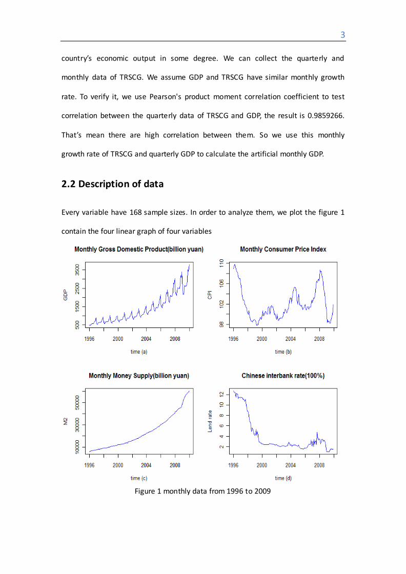
Every variable have 168 sample sizes. In order to analyze them, we plot the figure 1

contain the four linear graph of four variables

Figure 1 monthly data from 1996 to 2009

4

From the graph (a) of the figure 1, we can have that gross domestic product has a

steady growth in the overall. And the quantity of almost every January, February,

December have are decreased and that of every August, September, November are

increased. Since, there is a holiday on January or February, and the gross domestic

product is reduced. And at the end of year, gross domestic product is ascending.

From the graph (b) of the figure 1, we can have that the consumer price index stayed

more or less constant, except a sharp decreasing from1996 to 1997. Refer to the

relevant documentation, Chinese government introduced a new policy, allowing the

market to independent pricing, Prices increase are until the end of 1996, however,

Chinese economy has never appeared in a previously encountered problem:

deflation, the prices of many goods do not rise declined. This situation continued

until the end of 2004.

From the graph (c) of the figure 1, we can have that the money supply on the whole

has exponentially grown. The money supply from Jan 1996 to Dec 2009, the growth

from 5840.1billion to 60622.50 billion is an increase of 10 times.

From the graph (d) of the figure 1, we can have that Chinese interbank rate. From

1996 to 1998, it shows sharp decreasing, from 12.6% to 4.22%. Then trend of data is

almost stationary.

3. Modeling

3.1 Vector autoregression

Vector autoregression (VAR) is an econometric model used to capture the evolution

and the interdependencies between multiple time series, generalizing the univariate

5

AR models. All the variables in a VAR are treated symmetrically by including for each

variable an equation explaining its evolution based on its own lags and the lags of all

the other variables in the model. Based on this feature, Christopher Sims advocates

the use of VAR models as a theory-free method to estimate economic relationships,

thus being an alternative to the "incredible identification restrictions" in structural

models

A VAR model describes the evolution of a set of k variables (called endogenous

variables) over the same sample period (t = 1, ..., T) as a linear function of only their

past evolution. The variables are collected in a k × 1 vector yt, which has as the ith

element yi,t the time t observation of variable yi. For example, if the ith variable is

GDP, then yi,t is the value of GDP at t.

A (reduced) p-th order VAR, denoted VAR(p), is

yt = c + Φ1yt−1 +⋯ +Φp yt−p + εt

where c is a k × 1 vector of constants (intercept), Φi is a k × k matrix (for every i =

1, ..., p) and et is a k × 1 vector of error terms

The i-periods back observation yt−i is called the i-th lag of y. Thus, a pth-order VAR

is also called a VAR with p lags.

{yt} is covariance-stationary if Eyt and E(yt-Eyt)( yt−j-Eyt−j)’ are independent of t for

any j.

3.2 Transformation of data

To get a better result of fitting and make these four variables in the same order of

magnitude, we make appropriate transformations to GDP and M2, whose units are billion . And

the interbank rate and CPI stay the same.

6

Set gdpgrowth = 100 ∗ log GDP t

GDP t−1 (GDP growth rate)

mgrowth = 100 ∗ log M2 t

M2 t − 1 (M2 growth rate)

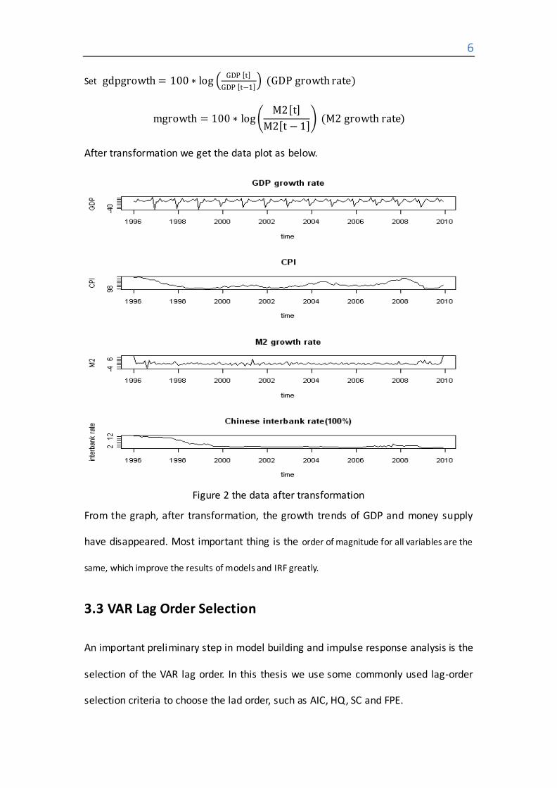
After transformation we get the data plot as below.

Figure 2 the data after transformation

From the graph, after transformation, the growth trends of GDP and money supply

have disappeared. Most important thing is the order of magnitude for all variables are the

same, which improve the results of models and IRF greatly.

3.3 VAR Lag Order Selection

An important preliminary step in model building and impulse response analysis is the

selection of the VAR lag order. In this thesis we use some commonly used lag-order

selection criteria to choose the lad order, such as AIC, HQ, SC and FPE.

7

Using Akaike Information Criterion to choose lag order.

AIC = −2 logL

T +

2k

T

Using Schwartz Criterion to choose lag order.

SC = −2 logL

T +

klogT

T

Using Hannan-Quinn to choose lag order

HQ = −2 logL

T + 2k

Ln (logT )

T

We use “VARselect” in R get the results below:

Base on AIC and FPE, the lag order we chosen is 12. Because the data we used are

monthly data, the result is reasonable. Base on SC and HQ, we will try the models

with lag order equal to 11 or 2 as well.

3.4 Models selection

In R, VAR model has four types: having trend, having constant, having both and

having none. According to the analysis above, we choose the type of having both.

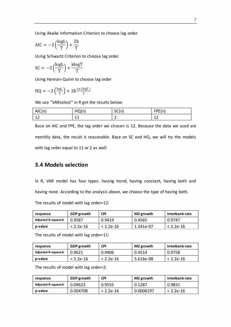
The results of model with lag order=12:

The results of model with lag order=11:

The results of model with lag order=2:

AIC(n) HQ(n) SC(n) FPE(n)

12 11 2 12

response GDP growth CPI M2 growth Interbank rate

Adjusted R-squared: 0.9587 0.9419 0.4565 0.9747

p-value < 2.2e-16 < 2.2e-16 1.541e-07 < 2.2e-16

response GDP growth CPI M2 growth Interbank rate

Adjusted R-squared: 0.9621 0.9406 0.4514 0.9758

p-value < 2.2e-16 < 2.2e-16 5.616e-08 < 2.2e-16

response GDP growth CPI M2 growth Interbank rate

Adjusted R-squared: 0.09623 0.9555 0.1287 0.9831

p-value 0.004708 < 2.2e-16 0.0006197 < 2.2e-16

8

Because the data we uesd are monthly data, the model with lag order being 12 has

more practical meaning than that with lag order being 11. What’s more, judging from

adjusted R-squared, the moder with lag order being 12 is better.

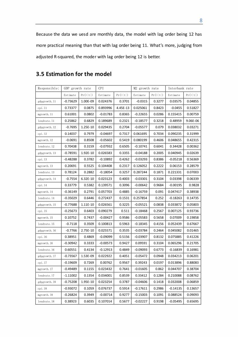
3.5 Estimation for the model

Responsible: GDP growth rate CPI M2 growth rate Interbank rate

Estimate Pr(>|t|) Estimate Pr(>|t|) Estimate Pr(>|t|) Estimate Pr(>|t|)

gdpgrowth.l1 -0.73629 1.00E-09 0.024376 0.3701 -0.0315 0.3277 0.03575 0.04855

cpi.l1 0.73377 0.0875 0.893996 4.45E-13 0.025061 0.8423 -0.0455 0.51827

mgrowth.l1 0.61001 0.0802 -0.01783 0.8365 -0.22655 0.0286 0.155415 0.00759

lendrate.l1 0.25862 0.6829 0.189689 0.2321 -0.18577 0.3218 0.48959 9.06E-06

gdpgrowth.l2 -0.7695 1.25E-10 0.029435 0.2704 -0.05577 0.079 0.038032 0.03271

cpi.l2 0.14037 0.7979 -0.04697 0.7317 0.061695 0.7034 0.090235 0.31999

mgrowth.l2 -0.0691 0.8508 -0.05602 0.5419 0.080199 0.4606 0.048655 0.42315

lendrate.l2 0.70438 0.3159 -0.07932 0.6505 -0.10741 0.6041 0.34428 0.00362

gdpgrowth.l3 -0.78591 1.92E-10 0.026583 0.3355 -0.04188 0.2005 0.040945 0.02639

cpi.l3 -0.48288 0.3782 -0.10892 0.4262 -0.03293 0.8386 -0.05218 0.56369

mgrowth.l3 0.20691 0.5525 0.104408 0.2317 0.126052 0.2222 0.06153 0.28579

lendrate.l3 0.78124 0.2882 -0.18054 0.3257 0.287244 0.1871 0.221331 0.07003

gdpgrowth.l4 -0.7554 6.32E-10 0.023123 0.4003 -0.03301 0.3104 0.03398 0.06339

cpi.l4 0.33779 0.5382 0.139571 0.3096 -0.00642 0.9684 -0.00195 0.9828

mgrowth.l4 -0.36149 0.2791 0.057703 0.4885 -0.16759 0.091 0.047417 0.38938

lendrate.l4 -0.35029 0.6446 0.272437 0.1531 0.257854 0.252 -0.18263 0.14735

gdpgrowth.l5 -0.77688 1.11E-10 0.026561 0.3225 -0.05521 0.0838 0.033872 0.05803

cpi.l5 -0.25673 0.6403 0.090279 0.511 -0.18468 0.2567 0.007125 0.93736

mgrowth.l5 0.10752 0.7437 -0.00427 0.9586 -0.05583 0.5658 0.07009 0.19858

lendrate.l5 -0.7118 0.3509 0.100813 0.5963 -0.18345 0.4156 0.052439 0.67667

gdpgrowth.l6 -0.7766 2.75E-10 0.025571 0.3535 -0.03784 0.2464 0.045082 0.01465

cpi.l6 0.38951 0.4869 -0.09099 0.5156 -0.03907 0.8132 0.075885 0.41226

mgrowth.l6 -0.30942 0.3333 -0.00573 0.9427 0.09591 0.3104 0.065296 0.21705

lendrate.l6 0.60551 0.4134 -0.12913 0.4849 -0.09093 0.6773 -0.16839 0.16981

gdpgrowth.l7 -0.73567 1.53E-09 0.022922 0.4051 -0.05472 0.0948 0.034213 0.06201

cpi.l7 -0.19609 0.7269 0.00762 0.9567 0.39243 0.0197 0.013896 0.88083

mgrowth.l7 -0.49489 0.1155 0.023432 0.7641 -0.01605 0.862 0.044707 0.38704

lendrate.l7 -1.11002 0.1354 0.034001 0.8539 0.33412 0.1284 0.210088 0.08762

gdpgrowth.l8 -0.75208 1.95E-10 0.023254 0.3787 -0.04606 0.1418 0.032008 0.06859

cpi.l8 -0.93072 0.1059 0.076737 0.5914 -0.17611 0.2986 -0.14135 0.13657

mgrowth.l8 -0.26824 0.3949 -0.00714 0.9277 -0.15003 0.1091 0.088524 0.09093

lendrate.l8 0.38923 0.6035 0.107014 0.5677 -0.02227 0.9198 -0.05495 0.65695

9

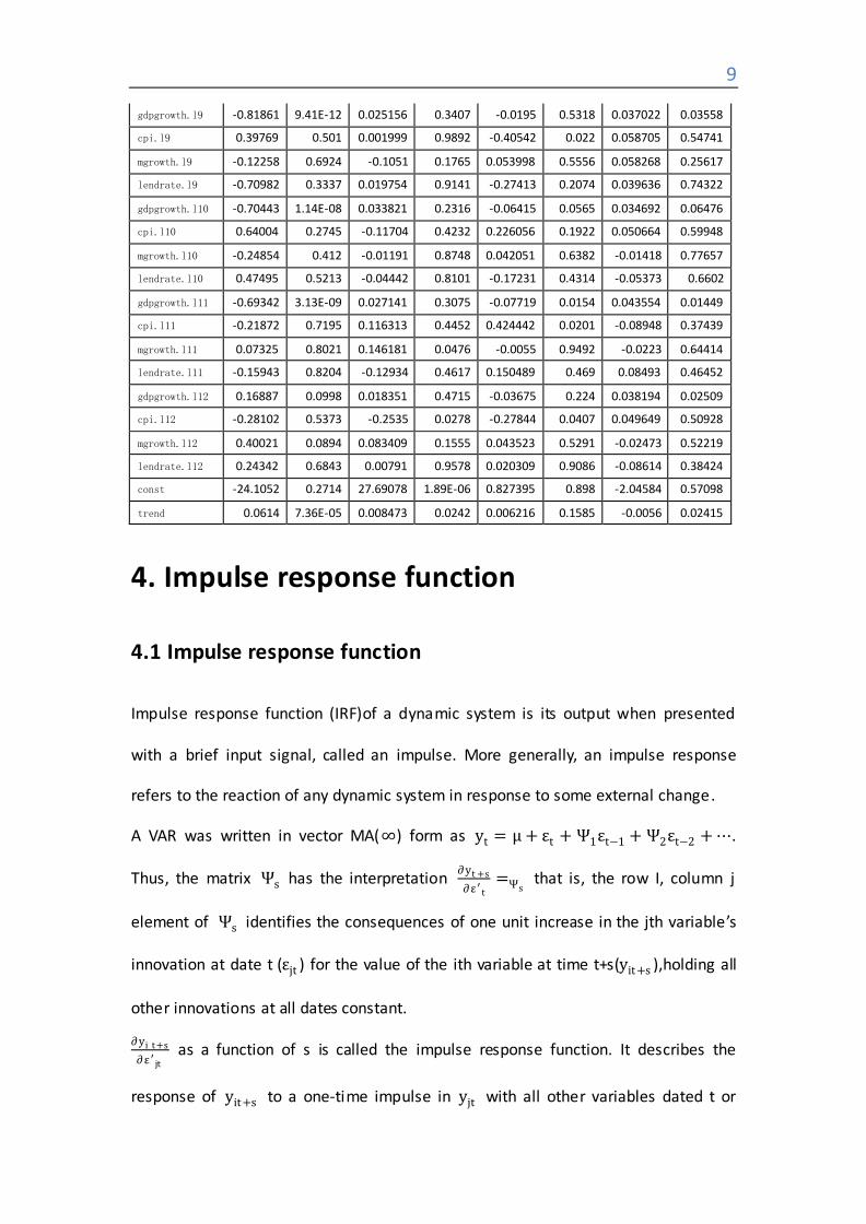
gdpgrowth.l9 -0.81861 9.41E-12 0.025156 0.3407 -0.0195 0.5318 0.037022 0.03558

cpi.l9 0.39769 0.501 0.001999 0.9892 -0.40542 0.022 0.058705 0.54741

mgrowth.l9 -0.12258 0.6924 -0.1051 0.1765 0.053998 0.5556 0.058268 0.25617

lendrate.l9 -0.70982 0.3337 0.019754 0.9141 -0.27413 0.2074 0.039636 0.74322

gdpgrowth.l10 -0.70443 1.14E-08 0.033821 0.2316 -0.06415 0.0565 0.034692 0.06476

cpi.l10 0.64004 0.2745 -0.11704 0.4232 0.226056 0.1922 0.050664 0.59948

mgrowth.l10 -0.24854 0.412 -0.01191 0.8748 0.042051 0.6382 -0.01418 0.77657

lendrate.l10 0.47495 0.5213 -0.04442 0.8101 -0.17231 0.4314 -0.05373 0.6602

gdpgrowth.l11 -0.69342 3.13E-09 0.027141 0.3075 -0.07719 0.0154 0.043554 0.01449

cpi.l11 -0.21872 0.7195 0.116313 0.4452 0.424442 0.0201 -0.08948 0.37439

mgrowth.l11 0.07325 0.8021 0.146181 0.0476 -0.0055 0.9492 -0.0223 0.64414

lendrate.l11 -0.15943 0.8204 -0.12934 0.4617 0.150489 0.469 0.08493 0.46452

gdpgrowth.l12 0.16887 0.0998 0.018351 0.4715 -0.03675 0.224 0.038194 0.02509

cpi.l12 -0.28102 0.5373 -0.2535 0.0278 -0.27844 0.0407 0.049649 0.50928

mgrowth.l12 0.40021 0.0894 0.083409 0.1555 0.043523 0.5291 -0.02473 0.52219

lendrate.l12 0.24342 0.6843 0.00791 0.9578 0.020309 0.9086 -0.08614 0.38424

const -24.1052 0.2714 27.69078 1.89E-06 0.827395 0.898 -2.04584 0.57098

trend 0.0614 7.36E-05 0.008473 0.0242 0.006216 0.1585 -0.0056 0.02415

4. Impulse response function

4.1 Impulse response function

Impulse response function (IRF)of a dynamic system is its output when presented

with a brief input signal, called an impulse. More generally, an impulse response

refers to the reaction of any dynamic system in response to some external change.

A VAR was written in vector MA(∞) form as yt = μ + εt + Ψ1εt−1 + Ψ2εt−2 +⋯.

Thus, the matrix Ψs has the interpretation ∂yt +s

∂ε′ t=Ψs

that is, the row I, column j

element of Ψs identifies the consequences of one unit increase in the jth variable’s

innovation at date t (εjt ) for the value of the ith variable at time t+s(yit +s ),holding all

other innovations at all dates constant.

∂yi t+s

∂ε′ jt as a function of s is called the impulse response function. It describes the

response of yit +s to a one-time impulse in yjt with all other variables dated t or

10

earlier held constant.

4.2 Empirical analysis:

The impulse response function of VAR is to analysis dynamic affects of the system

when the model received the impulse. As our VAR model, we have four variables. We

can work the response between these variables. In order to display the response

function clearer, we plot the chart as figure 4 and figure 5.

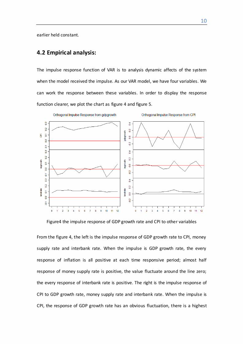
Figure4 the impulse response of GDP growth rate and CPI to other variables

From the figure 4, the left is the impulse response of GDP growth rate to CPI, money

supply rate and interbank rate. When the impulse is GDP growth rate, the every

response of inflation is all positive at each time responsive period; almost half

response of money supply rate is positive, the value fluctuate around the line zero;

the every response of interbank rate is positive. The right is the impulse response of

CPI to GDP growth rate, money supply rate and interbank rate. When the impulse is

CPI, the response of GDP growth rate has an obvious fluctuation, there is a highest

11

positive effect on the first month, lowest negative effect on the eighth month; the

response of money supply rate has an smooth fluctuation, there is more varied on

the second half year; almost response of interbank rate are positive except the first

month and the change is smooth.

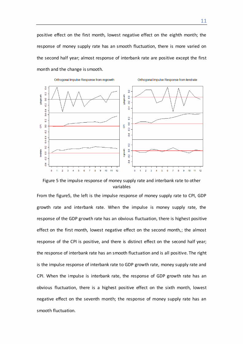
Figure 5 the impulse response of money supply rate and interbank rate to other variables

From the figure5, the left is the impulse response of money supply rate to CPI, GDP

growth rate and interbank rate. When the impulse is money supply rate, the

response of the GDP growth rate has an obvious fluctuation, there is highest positive

effect on the first month, lowest negative effect on the second month,; the almost

response of the CPI is positive, and there is distinct effect on the second half year;

the response of interbank rate has an smooth fluctuation and is all positive. The right

is the impulse response of interbank rate to GDP growth rate, money supply rate and

CPI. When the impulse is interbank rate, the response of GDP growth rate has an

obvious fluctuation, there is a highest positive effect on the sixth month, lowest

negative effect on the seventh month; the response of money supply rate has an

smooth fluctuation.

12

5. Testing procedures

5.1 Granger causality test

Granger causality test is a technique for determining whether one time series is

useful in forecasting another. Two causality tests are implemented. The first is a

F-type Granger-causality test and the second is a Wald-type test that is characterized

by testing for nonzero correlation between the error processes of the cause and

effect variables. Granger causality test can be applied in a multivariate context.

Suppose that the variables of a VAR are categorized into two groups, as represented

by the (n1*1) vector y1, and the (n2*1) vector y2. The VAR may then be written

y1t = c1 + A1′ x1t + A2

′ x2t + ε1t , y2t = c2 + B1′ x1t + B2

′ x2t + ε2t . The group of

variables represented by y1 is said to be block-exogenous in the time series sense

with respect to the variables in y2 if the element y2 in are of no help in improving a

forecast of any variable contained in y1 that is based on lagged values of all the

elements of y1 alone. In the VAR model above, y1 is block-exogenous when A2 = 0.

5.2 Testing analysis

Granger causality test is a technique for determining whether one time series is

useful in forecasting another. It can determine whether there is causality relationship

between variables. We work the Granger causality test, the result as following

table(confidence interval is 94%)

13

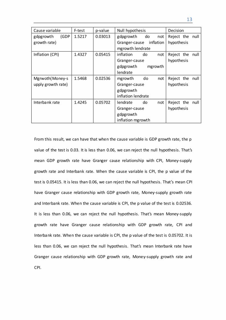
Cause variable F-test p-value Null hypothesis Decision

gdpgrowth (GDP

growth rate)

1.5217 0.03013 gdpgrowth do not

Granger-cause inflation

mgrowth lendrate

Reject the null

hypothesis

Inflation (CPI) 1.4327 0.05415 inflation do not

Granger-cause

gdpgrowth mgrowth

lendrate

Reject the null

hypothesis

Mgrwoth(Money-s

upply growth rate)

1.5468 0.02536 mgrowth do not

Granger-cause

gdpgrowth inflation lendrate

Reject the null

hypothesis

Interbank rate 1.4245 0.05702 lendrate do not

Granger-cause

gdpgrowth inflation mgrowth

Reject the null

hypothesis

From this result, we can have that when the cause variable is GDP growth rate, the p

value of the test is 0.03. It is less than 0.06, we can reject the null hypothesis. That’s

mean GDP growth rate have Granger cause relationship with CPI, Money-supply

growth rate and Interbank rate. When the cause variable is CPI, the p value of the

test is 0.05415. It is less than 0.06, we can reject the null hypothesis. That’s mean CPI

have Granger cause relationship with GDP growth rate, Money-supply growth rate

and Interbank rate. When the cause variable is CPI, the p value of the test is 0.02536.

It is less than 0.06, we can reject the null hypothesis. That’s mean Money-supply

growth rate have Granger cause relationship with GDP growth rate, CPI and

Interbank rate. When the cause variable is CPI, the p value of the test is 0.05702. It is

less than 0.06, we can reject the null hypothesis. That’s mean Interbank rate have

Granger cause relationship with GDP growth rate, Money-supply growth rate and

CPI.

14

6. Forecast

Forecasting is the process of estimation in unknown situations, which is commonly

used in discussion of time-series data. We use our VAR model to forecast the four

variables: GDP, CPI, M2, and interbank rate, the result as the following figure 6,

figuer7, figure 8, figure 9

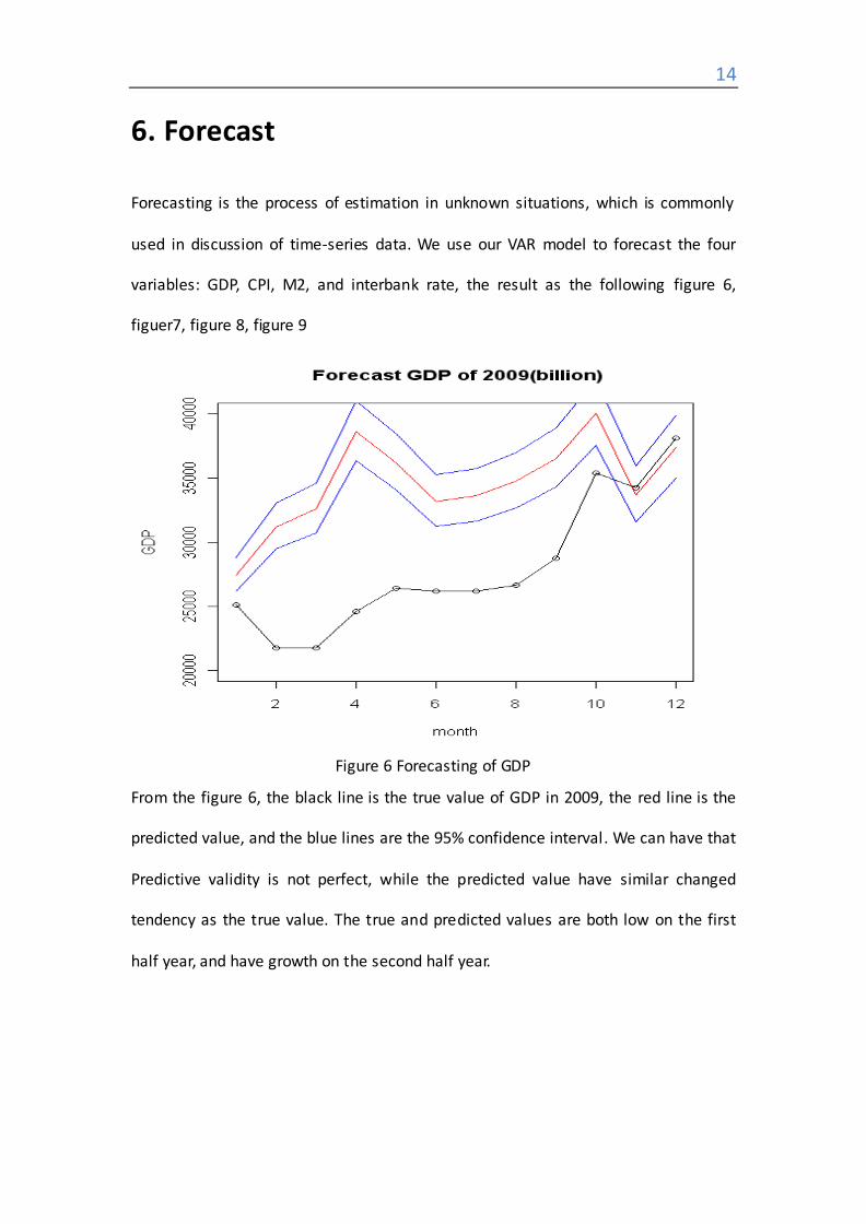
Figure 6 Forecasting of GDP

From the figure 6, the black line is the true value of GDP in 2009, the red line is the

predicted value, and the blue lines are the 95% confidence interval. We can have that

Predictive validity is not perfect, while the predicted value have similar changed

tendency as the true value. The true and predicted values are both low on the first

half year, and have growth on the second half year.

15

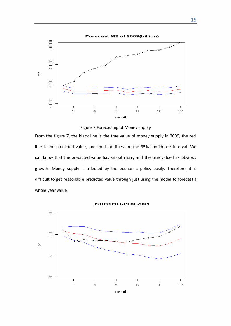
Figure 7 Forecasting of Money supply

From the figure 7, the black line is the true value of money supply in 2009, the red

line is the predicted value, and the blue lines are the 95% confidence interval. We

can know that the predicted value has smooth vary and the true value has obvious

growth. Money supply is affected by the economic policy easily. Therefore, it is

difficult to get reasonable predicted value through just using the model to forecast a

whole year value

16

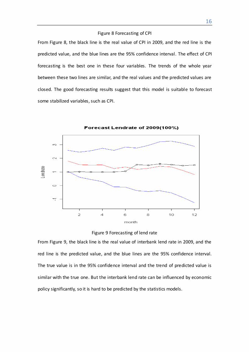
Figure 8 Forecasting of CPI

From Figure 8, the black line is the real value of CPI in 2009, and the red line is the

predicted value, and the blue lines are the 95% confidence interval. The effect of CPI

forecasting is the best one in these four variables. The trends of the whole year

between these two lines are similar, and the real values and the predicted values are

closed. The good forecasting results suggest that this model is suitable to forecast

some stabilized variables, such as CPI.

Figure 9 Forecasting of lend rate

From Figure 9, the black line is the real value of interbank lend rate in 2009, and the

red line is the predicted value, and the blue lines are the 95% confidence interval.

The true value is in the 95% confidence interval and the trend of predicted value is

similar with the true one. But the interbank lend rate can be influenced by economic

policy significantly, so it is hard to be predicted by the statistics models.

17

7 Conclusions

GDP growth rate does have an accelerative effect on CPI for the whole year. The

effects from GDP growth rate to money supply growth rate are obviously fluctuating,

more than a half time the effects are negative. GDP growth rate does have a very

smooth and positive effect on interbank rate for the whole year.

The effects from CPI to GDP growth rate are obviously fluctuating. There is a highest

positive effect on the first month, lowest negative effect on the eighth month. The

effects from CPI to money supply growth rate are smoothly fluctuating in first half

year, and more varied on the second half year. And CPI does have a smooth effect

around zero on interbank rate for the whole year.

The money supply growth rate has remarkable effect on the GDP growth rate and it

is about half positive effect except the second month, fourth month, sixth month and

tenth month. While, money supply growth rate has accelerated positive impact on

the CPI, it arrived at the highest value on the end of the year. Money supply growth

rate has smooth impact on interbank rate on the every month.

The interbank rate also has remarkable effect on the GDP growth rate and there is

positive and negative effects, has a highest positive value on the sixth month and

lowest negative value on the seventh month. Interbank rate has monotone effect on

CPI, it arrived at the highest value on the end of the year. Interbank rate has double

influence, the positive effect and negative effect distributed equably in the whole

year.

From the effects of forecasting these four variables, we get that predictive validity of

CPI and interbank lend rate are sound, the predictive value have similar trend as the

observation value of 2009, while the predictive validity of GDP and money supply are

18

not good. Both Money supply and interbank lend rate are affected by the economic

policy significantly. Therefore, it is not reasonable to use this model to forecast these

two variables money supply and interbank lend rate.

19

Reference

●Abdulnasser Hatemi-J(2004). Multivariate tests for autocorrelation in the stable

and unstable VAR models. Economic Modelling 21,p 85-115

●Achim Zeileis, Friedrich Leisch, Kurt Hornik, Christian Kleiber(2001).Strucchange: An

R Package for Testing for Structural Change in Linear Regression Models

●Blanchard Olivier.(1989).A Traditional Interpretation of Macroeconomic Fluctuations.

American economic review79,p46-64

●GUIDO M. KUERSTEINER (2005). Automatic inference for infinite order vector auto

regressions. Econometric Theory, 21, p661-668 James D. Hamilton (1994). Time Series Analysis. Princeton University Press.p291-336

●Geisser, Seymour (1 June 1993) . Predictive Inference: An Introduction. Chapman &

Hall, CRC Press. ISBN 0-412-03471-9.

●Huijun Sun,.The causes and tends of the Chinese CPI. Economic Theory and Practice,

no.4, 2008. ●Karamé F. & A. Olmedo(2007). Asymmetric (and symmetric) properties of impulse–

responses functions in Markov-switching structural VAR, mimeo.

●Karlsen H.(1990) A class of nonlinear time series models, PhD Thesis, University of

Bergen, Norway.

●Lutz Kilian(2001). Impulse response analysis in vector autoregressions with

unknown lag order. Journal of Forecastin. 20, 161-179.

●Teräsvirtä, T(1995). Modelling nonlinearity in US Gross National Product 1889–

1987.Empirical Economics 20, 577–597.

●Tong, H( 1990). Nonlinear Time Series: a Dynamical System Approach. Oxford

University Press.

●Wen-Cheng Lu, Jong-Rong Chen, I-Hsuan Tung(2009). Trends and Volatilities in

Heterogeneous Patent Quality in Taiwan. J. Technol. Manag. Innov. 2009, Volume 4,

Issue 2

Appendix: R codes

rm(lis t=ls (all=TRUE))

data=read.table("data.txt",header=T)

attach(data)

#transform data

n<-length(GDP)

gdpgrowth<-numeric(0)

20

mgrowth<-numeric(0)

for (i in 2:n) {

gdpgrowth[i-1]<-100*log(GDP[i]/GDP[i-1])

mgrowth[i -1]<-100*log(MoneyS[i]/MoneyS[i-1])

}

lendrate<-Lendrate[2:n]

cpi<-CPI[2:n]

data1 <- data.frame(gdpgrowth,cpi ,mgrowth,lendrate)

#plot

gdp<-ts(gdpgrowth,s tart=c(1996,1),end=c(2008,12),frequency=12)

cpi<-ts(CPI,start=c(1996,1),end=c(2008,12),frequency=12)

mg<-ts(mgrowth,start=c(1996,1),end=c(2008,12),frequency=12)

l r<-ts(Lendrate,start=c(1996,1),end=c(2008,12),frequency=12)

par(mfrow=c(4,1))

plot.ts (gdp,main="GDP growth rate",xlab="time",ylab="GDP")

plot.ts (cpi ,main="CPI",xlab="time",ylab="CPI")

plot.ts (mg,main="M2 growth rate",xlab="time",ylab="M2")

plot.ts (lr,main="Chinese interbank rate(100%)",ylab="interbank rate",xlab="time")

#model

VARselect(data1,lag.ma x=12,type="both")

m1=VAR(data1, p =12, type = "both")

summary(m1)

m2=VAR(data1, p =11, type = "both")

summary(m2)

m3=VAR(data1, p =2, type = "both")

summary(m3)

#test

causality(m1, cause = "gdpgrowth")

causality(m1, cause = "mgrowth")

causality(m1, cause = "cpi")

causality(m1, cause = "lendrate")

#i rf

impu1=irf(m1, impulse = "gdpgrowth", response = c("cpi", "mgrowth", "lendrate"), boot =FALSE,n.head=12)

impu2=irf(m1,impulse = "cpi", response = c("gdpgrowth", "mgrowth", "lendrate"),n.ahead = 12, boot =FALSE)

impu3=irf(m1,impulse = "mgrowth", response = c("cpi", "gdpgrowth", "lendrate"), n.ahead = 12,boot =FALSE)

impu4=irf(m1,impulse = "lendrate", response = c("cpi", "mgrowth", "gdpgrowth"),n.ahead = 12, boot =FALSE)

21

plot(impu1,xlim=seq(1,12))

axis(1,xaxp=seq(1,13))

plot(impu1)

plot(impu2)

plot(impu3)

plot(impu4)

#forecast

a=predict(m1, n.ahead = 12, ci = 0.95)

gdpp<-numeric(12)

gdppu<-numeric(12)

gdppl<-numeric(12)

m2p<-numeric(12)

m2pu<-numeric(12)

m2pl<-numeric(12)

cpip<-numeric(12)

cpipu<-numeric(12)

cpipl<-numeric(12)

lendp<-numeric(12)

lendpu<-numeric(12)

lendpl<-numeric(12)

for (i in 1:12){

gdpp[i ]<-exp(a$fcst$gdpgrowth[i ,1]/100)*34013.08

gdppu[i ]<-exp(a$fcst$gdpgrowth[i ,3]/100)*34013.08

gdppl [i]<-exp(a$fcst$gdpgrowth[i,2]/100)*34013.08

m2p[i]<-exp(a$fcst$mgrowth[i ,1]/100)*475166.6

m2pu[i]<-exp(a$fcst$mgrowth[i ,3]/100)*475166.6

m2pl[i ]<-exp(a$fcst$mgrowth[i,2]/100)*475166.6

cpip[i ]<-a$fcst$cpi[i ,1]

cpipu[i ]<-a$fcst$cpi[i ,3]

cpipl [i]<-a$fcst$cpi [i ,2]

lendp[i ]<-a$fcst$lendrate[i ,1]

lendpu[i]<-a$fcst$lendrate[i ,3]

lendpl[i ]<-a$fcst$lendrate[i,2]

}

data2=read.table("datat.txt",header=T)

plot(data2$GDP,main=" Forecast GDP of 2009(billion)",xlab="month",ylab="GDP",ylim=c(20000,40000))

lines(data2$GDP)

lines(gdpp,col=2)

lines(gdppu,col=4)

lines(gdppl,col=4)

22

plot(data2$MoneyS,main=" Forecast M2 of 2009(billion)",xlab="month",ylab="M2",ylim=c(450000,600000))

lines(data2$MoneyS)

lines(m2p,col=2)

lines(m2pu,col=4)

lines(m2pl ,col=4)

plot(data2$CPI,main=" Forecast CPI of 2009",xlab="month",ylab="CPI",ylim=c(90,105))

lines(data2$CPI)

lines(cpip,col=2)

lines(cpipu,col=4)

lines(cpipl,col=4)

plot(data2$Lendrate,main=" Forecast Lendrate of 2009(100%)",xlab="month",ylab="Lendrate",ylim=c( -1.5,3.5))

lines(data2$Lendrate)

lines(lendp,col=2)

lines(lendpu,col=4)

lines(lendpl ,col=4)