Embed Size (px)
Citation preview
Imputation Methods for Handling Item-Nonresponse in the Social Sciences: A
Methodological Review
Gabriele B. Durrant
ESRC National Centre for Research Methods and Southampton Statistical Sciences Research Institute
(S3RI), University of Southampton
NCRM Methods Review Papers
NCRM/002
Imputation Methods for Handling Item-Nonresponse in the Social Sciences: A
Methodological Review
Gabriele B. Durrant1 ESRC National Centre for Research Methods and Southampton Statistical Sciences Research Institute
(S3RI), University of Southampton
June 2005
Abstract:
Missing data are often a problem in social science data. Imputation methods fill in the missing
responses and lead, under certain conditions, to valid inference. This article reviews several
imputation methods used in the social sciences and discusses advantages and disadvantages of these
methods in practice. Simpler imputation methods as well as more advanced methods, such as
fractional and multiple imputation, are considered. The paper introduces the reader new to the
imputation literature to key ideas and methods. For those already familiar with imputation methods
the paper highlights some new developments and clarifies some recent misconceptions in the use of
imputation methods. The emphasis is on efficient hot deck imputation methods, implemented in
either multiple or fractional imputation approaches. Software packages for using imputation
methods in practice are reviewed highlighting newer developments. The paper discusses an
example from the social sciences in detail, applying several imputation methods to a missing
earnings variable. The objective is to illustrate how to choose between methods in a real data
example. A simulation study evaluates various imputation methods, including predictive mean
matching, fractional and multiple imputation. Certain forms of fractional and multiple hot deck
methods are found to perform well with regards to bias and efficiency of a point estimator and
robustness against model misspecifications. Standard parametric imputation methods are not found
adequate for the application considered.
Keywords: item-nonresponse, imputation, fractional imputation, multiple imputation, estimation of
distribution functions.
1 Gabriele B. Durrant, ESRC National Centre for Research Methods and Southampton Statistical Sciences Research Institute (S3RI), University of Southampton
Contents
1. Introduction
2. Missing Data Approaches
3. Notation and Typology of Item-Nonresponse
4. Imputation Methods
4.1 Simple Imputation Methods
4.2 Regression Imputation
4.3 Hot Deck Imputation Methods
4.4 Nearest-Neighbour Imputation
4.5 Predictive Mean Matching Imputation
4.6 Repeated Imputation: Multiple and Fractional Imputation
4.6.1 Multiple Imputation
4.6.2 Fractional Imputation
4.7 Debate on Single, Fractional and Multiple Imputation: A Note of Caution
5. Software for Imputation
6. Case Study: Estimating Pay Distributions in the Presence of Missing Data
6.1 Example from the UK Labour Force Survey
6.2 Imputation Approaches for LFS Application
7. Simulation Study
8. Conclusions References
1. Introduction
In sample surveys nonresponse is often a major problem. This is of particular concern in medical
and social science data. Many researchers in the social sciences are often faced with nonresponse
problems but may not be familiar with statistical analysis methods that address the missing data
problem adequately. Often the key focus of the research is not the nonresponse itself, which may be
regarded as a nuisance, but a substantial research question, such as the estimation of income
distributions or the estimation of regression models to analyse economic or demographic data
(Lillar et al., 1986; Freedman and Wolf, 1995, Stuttard and Jenkins, 2001; Hirsch and Schumacher,
2004). Variables of interest to social scientists, such as income variables, opinion and attitudes,
beliefs and others might be regarded as sensitive questions and are therefore often prone to
nonresponse. Dealing with nonresponse can be a difficult matter and it is important to apply
adequate missing data methods to obtain valid inference.
This article reviews various imputation methods used within the social sciences to compensate for
item-nonresponse bias, and provides guidance on how to use such methods in practice. A case study
from the social sciences is presented, illustrating the choice of imputation methods for a particular
application. Simple imputation methods are commonly used within the social sciences but these
may not be adequate in many circumstances (Ibrahim et al. 2005). More sophisticated methods,
such as fractional hot deck, multiple imputation and generally less parametric methods, have
advantages and the use of such advanced methods may be preferable. In this paper, the application
of hot deck methods is emphasised as a means of relaxing distributional assumptions made by
standard parametric imputation methods, such as regression and parametric multiple imputation. It
also discusses a method combining hot deck and multiple imputation as a semi-parametric
approach. The paper introduces the novice to the principles, methods and recent debates in the
imputation literature. It also provides the reader familiar with imputation methods with newer
developments in this field. A review of recent software developments from a social sciences
perspective is included. This article addresses some recent misconceptions with respect to the use of
proper and improper (multiple) imputation. It is emphasised that the choice of an appropriate
imputation method may strongly depend on the data available, the application and purpose of the
analysis, as illustrated in an example from the social sciences.
The article is structured as follows. In section 2, different approaches to handling missing data are
presented briefly. Definitions and basic assumptions about the missing data mechanisms are
introduced in section 3. In section 4, several imputation methods as a way of handling nonresponse
are reviewed. The problem of valid variance estimation under imputation is addressed briefly,
however, this is not the focus of the paper. Section 5 reviews software for imputation in practice. A
case study from the social sciences is discussed in section 6. A simulation study in section 7
evaluates different imputation methods with regards to bias and efficiency of a point estimator and
robustness under model misspecification. Some concluding remarks are made in section 8.
2. Missing Data Approaches
By nonresponse it is meant that the required data are not obtained for all elements, which are
selected for observation. Generally, a distinction is made between unit nonresponse, i.e. the failure
of a selected sample member to respond, and item nonresponse where it is failed to obtain some
required information from individual sample members. Unit nonresponse occurs if it is not possible
to interview certain sample members or if sample members did not want to take part in the survey.
Item nonresponse on the other hand occurs if the interviewer fails to ask a question, does not record
the answer or the sample member refuses to answer a question or does not know the answer. There
are several ways of dealing with nonresponse problems. For unit nonresponse normally weighting
methods are applied. To compensate for item nonresponse a range of missing data methods exist,
such as available case method, imputation methods, weighting methods and model-based
procedures such as maximum likelihood estimation. Overviews of such methods are given in Little
and Rubin (1990), GSS (1996), Schafer and Graham (2002), Raghunathan (2004) and Ibrahim et al.
(2005). The focus of this paper is on imputation methods to compensate for item-nonresponse.
Nonresponse occurring in longitudinal studies, such as attrition or drop-out, will not be considered.
Some simple methods that are commonly used to handle item-nonresponse are listwise or case
deletion, pairwise deletion and available case analysis which focus on observed cases only (Allison,
2001; Ibrahim et al. 2005). Although these methods are sometimes applied by social scientists they
have several shortcomings which are reported in Schafer and Graham (2002) and Allison (2001).
Such methods are usually found not adequate to compensate for nonresponse bias in particular
when estimating parameters other than means and may only be valid under strong assumptions
about the mechanism that generated the missing values. In addition, variance estimation may not be
straightforward and relationships between variables may be distorted. Maximum likelihood
methods to address nonresponse problems have been described in Little and Rubin (2002) and
Allison (2001). Weighting methods, such as propensity score weighting, although commonly used
in the design and analysis of surveys, can also be used to adjust for item-nonresponse, as discussed
in David et al. (1983), Little (1986) and Little and Rubin (2002). Improved weighting approaches,
relaxing distributional assumptions and improving efficiency, have been proposed by Robins,
Rotnitzky and Zhao (1994) and Robins and Rotnitzky (1995). Alternative approaches, regarding the
missing data problem as an identification problem, have been discussed in Manksi (1995), and
Manski (2005). However, these methods will not be reviewed here for space reasons.
3. Notation and Typology of Item-Nonresponse
Different types of item-nonresponse can be distinguished. In general, the missing-data pattern can be
univariate, that means that the missing values only occur in a single response variable, or multivariate in
the sense that missing values occur in more than one variable. The choice of imputation method may
depend on the underlying missing data pattern such that the investigation of the nonresponse pattern is
important and useful. To facilitate the discussion the following notation is introduced. Let U be a finite
population of N units and s a sample of sample size n . Let H denote the complete data matrix with
element ikh in the ith row and kth column, where 1,...,i n= , and 1,...,k K= . In the presence of
missing data obsH refers to the observed part of the matrix H and misH to the missing part. Let R
denote a matrix with elements
⎧⎪⎪= ⎨⎪⎪⎩
if observed1
0 if missing.ik
ikik
hr
h (1)
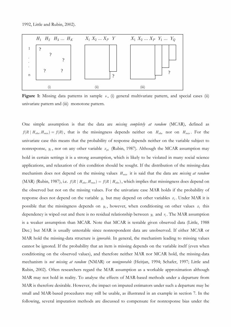
This general multivariate missing data pattern is illustrated in figure 1 (i) (Little and Rubin, 1990). For
the simple univariate case, where only one variable is subject to nonresponse and all other variables are
fully observed, let iy for unit i denote the sample value of the variable subject to missing data, ir a
binary indicator of whether iy is observed and ix a vector of fully observed auxiliary variables,
1 2( , ,..., )i i i Pix x x x= , with 1,...,p P= , to be able to distinguish easily between partially and fully
observed variables, as illustrated in figure 1 (ii). The notation Y denotes a vector and X a matrix of
values respectively. For the case, where several variables are subject to nonresponse we may refer to
1 2, ,...,i i Qiy y y , 1,...,q Q= , and we have several indicator variables 1 ,...,i Qir r . It is then ( , )i i ih x y= . A
particular missing data pattern is a monotone nonresponse where the variables subject to missing data can
be arranged in such a way that qy is observed whenever 1qy + is observed, for all 1,..., 1q Q= − , also
illustrated in figure 1 (iii).
One major problem with missing data is that it is usually unknown how nonresponse for each variable
is generated, i.e. the distribution ( | )f R H , referred to as the nonresponse mechanism, where f
denotes the probability density function, is unknown. It is usually necessary to make assumptions about
this distribution, which often cannot be verified (Kalton, 1983; Nordholt, 1998; Lessler and Kalsbeek,
1992, Little and Rubin, 2002).
Figure 1: Missing data patterns in sample s , (i) general multivariate pattern, and special cases (ii)
univariate pattern and (iii) monotone pattern.
One simple assumption is that the data are missing completely at random (MCAR), defined as
( | , ) ( )obs misf R H H f R= , that is the missingness depends neither on obsH nor on misH . For the
univariate case this means that the probability of response depends neither on the variable subject to
nonresponse, iy , nor on any other variable pix (Rubin, 1987). Although the MCAR assumption may
hold in certain settings it is a strong assumption, which is likely to be violated in many social science
applications, and relaxation of this condition should be sought. If the distribution of the missing-data
mechanism does not depend on the missing values misH it is said that the data are missing at random
(MAR) (Rubin, 1987), i.e. ( | , ) ( | )obs mis obsf R H H f R H= , which implies that missingness does depend on
the observed but not on the missing values. For the univariate case MAR holds if the probability of
response does not depend on the variable iy but may depend on other variables ix . Under MAR it is
possible that the missingness depends on iy , however, when conditioning on other values ix this
dependency is wiped out and there is no residual relationship between iy and ir . The MAR assumption
is a weaker assumption than MCAR. Note that MCAR is testable given observed data (Little, 1988
Dec.) but MAR is usually untestable since nonrespondent data are unobserved. If either MCAR or
MAR hold the missing-data structure is ignorable. In general, the mechanism leading to missing values
cannot be ignored. If the probability that an item is missing depends on the variable itself (even when
conditioning on the observed values), and therefore neither MAR nor MCAR hold, the missing-data
mechanism is not missing at random (NMAR) or nonignorable (Heitjan, 1994; Schafer, 1997; Little and
Rubin, 2002). Often researchers regard the MAR assumption as a workable approximation although
MAR may not hold in reality. To analyse the effects of MAR-based methods under a departure from
MAR is therefore desirable. However, the impact on imputed estimators under such a departure may be
small and MAR-based procedures may still be usable, as illustrated in an example in section 7. In the
following, several imputation methods are discussed to compensate for nonresponse bias under the
1 2 ... PX X X Y
(i)
1 . . . n
1 2 1... ...P QX X X Y Y
(ii)
? ? ? ? ?
1 2 3 ... KH H H H
(iii)
? ?
MAR assumption.
4. Imputation Methods
Imputation is a method to fill in missing data with plausible values to produce a complete data set. A
distinction may be made between deterministic and stochastic (or random) imputation methods. Given a
selected sample deterministic methods always produce the same imputed value for units with the same
characteristics. Stochastic methods may produce different values. Usually, imputation makes use of a
number of auxiliary variables that are statistically related to the variable in which item nonresponse
occurs by means of an imputation model (Lessler and Kalsbeek, 1992; Schafer, 1997). The main reason for
carrying out imputation is to reduce nonresponse bias, which occurs because the distribution of the
missing values, assuming it was known, generally differs from the distribution of the observed items.
When imputation is used, it is possible to recreate a balanced design such that procedures used for
analysing complete data can be applied in many situations. Rather than deleting cases that are subject to
item-nonresponse the sample size is maintained resulting in a potentially higher efficiency than case
deletion. Imputation usually makes use of observed auxiliary information for cases with nonresponse
maintaining high precision (Schafer and Graham, 2002). However, it can have serious negative impacts
if imputed values are treated as real values. To estimate the variance of an estimator subject to
imputation adequately, often special adjustment methods are necessary to correct for the increase in
variability due to nonresponse and imputation. It is also possible to increase the bias by using
imputation, e.g. if the relationship between known and unknown variables is poor (Kalton and
Kasprzyk, 1982; Kalton, 1983; Särndal, Swensson and Wretman, 1992; Little and Rubin, 2002).
Under imputation let .Y denote the vector of imputed and observed values of Y in the univariate case,
such that
.iy = for 1
for 0
i i
Ii i
y r
y r
=⎧⎪⎪⎪⎨⎪ =⎪⎪⎩ , (2)
where i s∈ and Iiy denotes the imputed value for nonrespondent i . For the multivariate case the
notation 1 2. , . ,..., .KH H H is similarly used to denote the imputed vectors in H , or in short ( , . )obs misH H .
Let θ denote the parameter of interest in the population, e.g. a mean or a regression coefficient, which
is a function of the data in the population, and θ an estimator of θ based on the sample in the case of
full response, such that ˆ ( )Hθ θ= . Applying imputation in the case of nonresponse an estimator is
obtained of the form ˆ ˆ. ( , . )obs misH Hθ θ= called the imputed estimator. The aim is to define an
approximately unbiased and efficient estimator by choosing an appropriate imputation method.
Another important aspect of an imputation method is its robustness under misspecification of
underlying assumptions, such as assumptions about the imputation or the nonresponse model. When
choosing among imputation procedures it is important to consider carefully the type of analysis that
needs to be conducted. In particular, it should be distinguished if the goal is to produce efficient
estimates of means, totals, proportions or other official aggregated statistics, or a complete micro-data
file that can be used for a variety of different analyses. Other issues when choosing an imputation
method are the availability of variance estimation formulae and practical questions concerning
implementation and computing time. Further evaluation criteria of imputation methods are described
in Chambers (2003).
It needs to be stressed that standard variance estimation for a point estimator valid for complete data
may lead in many cases to severe underestimation of the true variance if applied to observed and
imputed data (Rao and Shao, 1992). Standard variance estimation techniques are therefore not adequate
in the presence of imputation. Various ways exist for estimating the variance of an estimator under
imputation, including multiple imputation (Rubin, 1987), two-phase approaches (Rao and Sitter, 1995;
Shao and Steel, 1999), model-assisted approaches (Deville and Särndal, 1994; Chen and Shao, 2000)
and replication methods, such as jackknife variance estimators (Rao and Shao, 1992; Shao and Sitter,
1996, Rao and Shao, 1999; Yung and Rao, 2000; Skinner and Rao, 2002). Recently, some
misconceptions about the use and applicability of certain types of imputation methods have been
mentioned in the literature, in particular with regards to estimation of the variance under imputation.
These will be addressed in section 4.6.
4.1. Simple Imputation Methods
There are a number of different approaches to imputation. Deductive methods impute a missing value by
using logical relations between variables and derive a value for the missing item with high probability
(GSS, 1996). The method of (unconditional) mean imputation imputes the overall mean of a numeric
variable for each missing item within that variable. A variation of this method is to impute a class mean,
where the classes may be defined based on some explanatory variables. Disadvantages of such
procedures are that distributions of survey variables are compressed and relationships between
variables may be distorted (Kalton, 1983; Lessler and Kalsbeek, 1992; Little and Rubin, 2002).
Although such simple imputation methods are commonly used in the social sciences (Jinn and
Sedransk, 1989; Allison, 2001) they are often not adequate to handle the missing data problem and
more sophisticated methods should be used.
4.2. Regression Imputation
Another broad class of methods for imputing missing data is regression imputation (Kalton and
Kasprzyk, 1982; Lessler and Kalsbeek, 1992; Little and Rubin, 2002). Predictive regression imputation, also
called deterministic regression or conditional mean imputation, involves the use of one or more auxiliary
variables, of which the values are known for complete units and units with missing values in the
variable of interest. A regression model is fitted that relates iy to auxiliary variables ix , i.e. the imputation
model. The predicted values are used for imputation of the missing values in Y . Usually, linear
regression is used for numeric variables, whereas for categorical data logistic regression may be used. A
potential disadvantage of predictive regression imputation is that it distorts the shape of the distribution
of the variable Y and the correlation between variables, which are not used in the regression model.
The distortion is particularly disturbing if the tails of the distribution are being studied. It might also
artificially inflate the statistical association between Y and the auxiliary variables. For example imputing
conditional means for missing income underestimates the percentages of cases in poverty even under
MCAR (Kalton, 1983).
Under random regression imputation, sometimes referred to as imputing from a conditional distribution, the
imputed value for the variable Y is a random draw from the conditional distribution of Y given X . If
a linear model between Y and X is considered a residual term is added to the predicted value from the
regression, which allows for randomisation and reflects uncertainty in the predicted value. This residual
can be obtained in different ways, e.g. by drawing from a normal distribution, either overall or within
subclasses, or by computing the regression residuals from the complete cases and selecting an observed
residual at random for each nonrespondent. A random regression model maintains the distribution of
the variables and allows for the estimation of distributional quantities (Kalton and Kasprzyk, 1982;
Kalton, 1983; Nordholt, 1998). An advantage of regression imputation is that it can make use of many
categorical and numeric variables. The method performs well for numeric data, especially if the variable
of interest is strongly related to auxiliary variables. The imputed value, however, is a predicted value
either with or without an added on residual and not an actually observed value as in so-called hot deck
methods. This can be a problem for imputing certain types of variables such as earnings and income
variables, which is illustrated in sections 6 and 7. Another potential disadvantage of such a parametric
approach is that the method may be sensitive to model misspecification of the regression model
(Schenker and Taylor, 1996). If the regression model is not a good fit the predictive power of the
model might be poor (Little and Rubin, 2002). The following hot deck imputation methods, which are
non-parametric or semi-parametric, may address some of these issues.
4.3. Hot Deck Imputation Methods
Many approaches have been developed that assign the value from a record with an observed item, the
donor, to a record with a missing value on that item, the recipient. Such imputation methods are
referred to as donor or hot deck methods, setting *Ij iy y= for some donor respondent *i for which
* 1ir = , 0jr = (Kalton and Kasprzyk, 1982; Little, 1986; Lessler and Kalsbeek, 1992). This involves
consideration of how best to select the donor value. A simple way is to impute for each missing item
the response of a randomly selected case for the variable of interest. Alternatively, imputation classes can
be constructed, selecting donor values at random within classes. Such classes may be defined based on
the crossclassification of fully observed auxiliary variables. An advantage of the method is that actually
occurring values are used for imputation. Hot deck imputation is therefore common in practice, and is
suitable when dealing with categorical data. Hot deck methods are usually non-parametric (or semi-
parametric) and aim to avoid distributional assumptions. This is important if components of the data
are skewed or show certain features, such as truncation and rounding effects, often the case for social
science data, or if the estimation of distributional quantities is of interest. Under hot deck imputation
the imputed values will have the same distributional shape as the observed data (Rubin, 1987). For a
hot deck method to work well a reasonably large sample size may be required.
4.4. Nearest-Neighbour Imputation
Nearest-neighbour imputation, also called distance function matching, is a donor method where the donor is
selected by minimising a specified ‘distance’ (Kalton, 1983; Lessler and Kalsbeek, 1992; Rancourt, 1999;
Chen and Shao, 2000 and 2001). This method involves defining a suitable distance measure, where the
distance is a function of the auxiliary variables. The observed unit with the smallest distance to the
nonrespondent unit is identified and its value is substituted for the missing item according to the
variable of concern. The easiest way is to consider just one continuous auxiliary variable 1X and to
compute the distance D from all respondents to the unit with the missing item, i.e. 1 1| |ji j iD x x= − ,
where j denotes the unit with the missing item in Y , 0jr = , and 1ir = . The missing item is replaced
by the value *iy , where the respondent *i is the donor for nonrespondent j if * 1 1min | |j iji iD x x= − .
An advantage of nearest neighbour imputation is that actually observed values are used for imputation.
Another advantage may be that if the cases are ordered for example geographically it introduces
geographical effects. However, it should be noted that the outcome could depend on the chosen order
of the file. Chen and Shao (2000) prove that the nearest-neighbour approach, although a deterministic
method, estimates distributions correctly. Some values might be used several times for imputation if
more than one missing value occurs in a row, others may not be used at all. The variance of .( )yθ under
nearest neighbour imputation may be inflated if certain donors are used much more frequently than
others. The multiple usage of donors can be penalised or restricted to a certain number of times a
donor is selected for imputation. For example, the distance function can be defined as =*jiD
1 1min{| | (1 )}j i iix x tμ− ∗ + , where +∈μ is the assigned penalty for each usage, it is the number of
times the respondent i has already been used as a donor, = 0ir and =( ) 1d ir (Kalton, 1983).
4.5. Predictive Mean Matching Imputation
A hot-deck imputation approach that makes use of the regression or imputation model, discussed in
section 4.2, is the method of predictive mean matching imputation and has been described in Little (1988,
July), Heitjan and Little (1991), Heitjan and Landis (1994) and Durrant and Skinner (2005a). In its
simplest form it is nearest neighbour imputation where the distance is defined based on the predicted
values of iy from the imputation model, denoted iy . Predictive mean matching is essentially a
deterministic method. Randomisation can be introduced by defining a set of values that are closest to
the predicted value and choosing one value out of that set at random for imputation (Schenker and
Taylor, 1996; Nordholt, 1998; Little and Rubin, 2002). Another form of predictive mean matching
imputation is hot deck imputation within classes where the classes are defined based on the range of
the predicted values from the imputation model. This method achieves a more even spread of donor
values for imputation within classes, which reduces the variance of the imputed estimator. Donor
values within classes may be drawn with or without replacement, where without replacement is
expected to lead to a further reduction in the variance (Durrant and Skinner, 2005a; Kim and Fuller,
2004). The method of predictive mean matching is an example of a composite method, combining
elements of regression, nearest-neighbour and hot deck imputation. Since it is a semi-parametric
method, which makes use of the imputation model but does not fully rely on it, it is also assumed to be
less sensitive to misspecifications of the underlying model than for example regression imputation
(Schenker and Taylor, 1996).
For simplicity, some of the imputation methods have been explained in the univariate missing data
context. However, the methods presented may be extended to more general missing data patterns. In a
monotone missing data set up it may be possible to apply the imputation methods to 1,..., QY Y subject
to missing data sequentially. For example, in the case of regression imputation one can formulate the
imputation process as a sequence of regression models regressing qY on 1 1,..., ,qY Y X− for 1,...,q Q= .
However, imputation may be difficult to implement in multivariate settings.
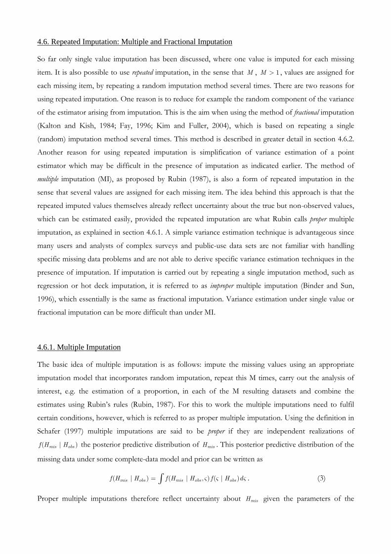
4.6. Repeated Imputation: Multiple and Fractional Imputation
So far only single value imputation has been discussed, where one value is imputed for each missing
item. It is also possible to use repeated imputation, in the sense that M , 1M > , values are assigned for
each missing item, by repeating a random imputation method several times. There are two reasons for
using repeated imputation. One reason is to reduce for example the random component of the variance
of the estimator arising from imputation. This is the aim when using the method of fractional imputation
(Kalton and Kish, 1984; Fay, 1996; Kim and Fuller, 2004), which is based on repeating a single
(random) imputation method several times. This method is described in greater detail in section 4.6.2.
Another reason for using repeated imputation is simplification of variance estimation of a point
estimator which may be difficult in the presence of imputation as indicated earlier. The method of
multiple imputation (MI), as proposed by Rubin (1987), is also a form of repeated imputation in the
sense that several values are assigned for each missing item. The idea behind this approach is that the
repeated imputed values themselves already reflect uncertainty about the true but non-observed values,
which can be estimated easily, provided the repeated imputation are what Rubin calls proper multiple
imputation, as explained in section 4.6.1. A simple variance estimation technique is advantageous since
many users and analysts of complex surveys and public-use data sets are not familiar with handling
specific missing data problems and are not able to derive specific variance estimation techniques in the
presence of imputation. If imputation is carried out by repeating a single imputation method, such as
regression or hot deck imputation, it is referred to as improper multiple imputation (Binder and Sun,
1996), which essentially is the same as fractional imputation. Variance estimation under single value or
fractional imputation can be more difficult than under MI.
4.6.1. Multiple Imputation
The basic idea of multiple imputation is as follows: impute the missing values using an appropriate
imputation model that incorporates random imputation, repeat this M times, carry out the analysis of
interest, e.g. the estimation of a proportion, in each of the M resulting datasets and combine the
estimates using Rubin’s rules (Rubin, 1987). For this to work the multiple imputations need to fulfil
certain conditions, however, which is referred to as proper multiple imputation. Using the definition in
Schafer (1997) multiple imputations are said to be proper if they are independent realizations of
( | )mis obsf H H the posterior predictive distribution of misH . This posterior predictive distribution of the
missing data under some complete-data model and prior can be written as
( | ) ( | , ) ( | )mis obs mis obs obsf H H f H H f H dς ς ς= ∫ . (3)
Proper multiple imputations therefore reflect uncertainty about misH given the parameters of the
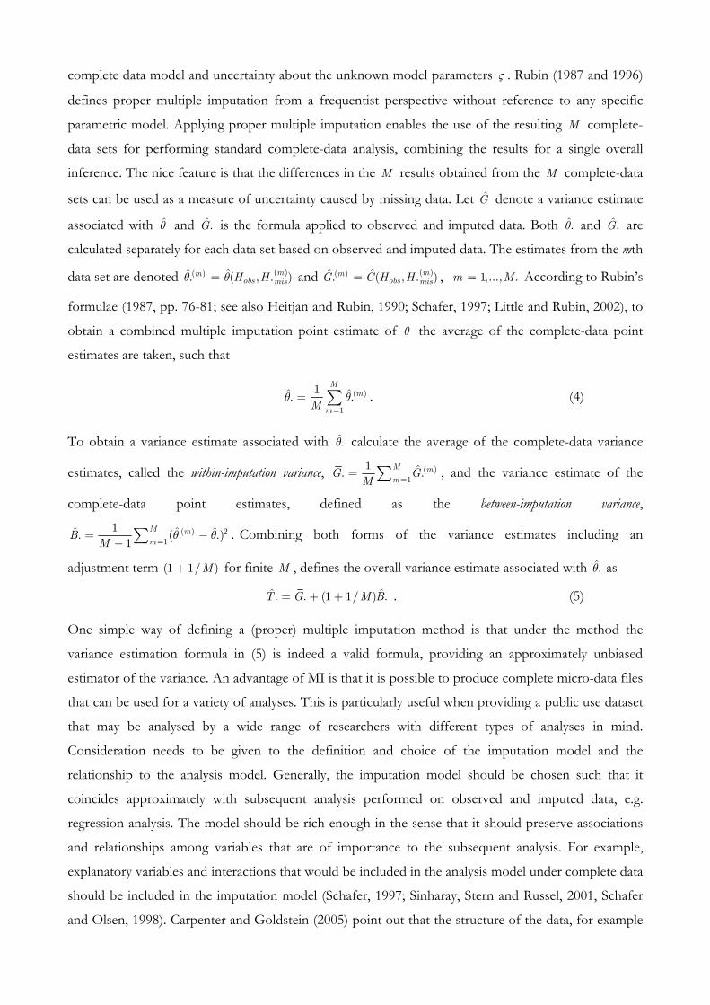
complete data model and uncertainty about the unknown model parameters ς . Rubin (1987 and 1996)
defines proper multiple imputation from a frequentist perspective without reference to any specific
parametric model. Applying proper multiple imputation enables the use of the resulting M complete-
data sets for performing standard complete-data analysis, combining the results for a single overall
inference. The nice feature is that the differences in the M results obtained from the M complete-data
sets can be used as a measure of uncertainty caused by missing data. Let G denote a variance estimate
associated with θ and ˆ.G is the formula applied to observed and imputed data. Both .θ and ˆ.G are
calculated separately for each data set based on observed and imputed data. The estimates from the mth
data set are denoted ( )( )ˆ ˆ. ( , . )mmobs misH Hθ θ= and ( )( )ˆ ˆ. ( , . )mm
obs misG G H H= , 1,..., .m M= According to Rubin’s
formulae (1987, pp. 76-81; see also Heitjan and Rubin, 1990; Schafer, 1997; Little and Rubin, 2002), to
obtain a combined multiple imputation point estimate of θ the average of the complete-data point
estimates are taken, such that
( )
1
1ˆ ˆ. .M
m
mMθ θ
== ∑ . (4)
To obtain a variance estimate associated with .θ calculate the average of the complete-data variance
estimates, called the within-imputation variance, ( )1
1 ˆ. .M mm
G GM =
= ∑ , and the variance estimate of the
complete-data point estimates, defined as the between-imputation variance,
( ) 21
1ˆ ˆ ˆ. ( . .)1
M mm
BM
θ θ=
= −− ∑ . Combining both forms of the variance estimates including an
adjustment term (1 1/ )M+ for finite M , defines the overall variance estimate associated with .θ as
ˆˆ. . (1 1/ ) .T G M B= + + . (5)
One simple way of defining a (proper) multiple imputation method is that under the method the
variance estimation formula in (5) is indeed a valid formula, providing an approximately unbiased
estimator of the variance. An advantage of MI is that it is possible to produce complete micro-data files
that can be used for a variety of analyses. This is particularly useful when providing a public use dataset
that may be analysed by a wide range of researchers with different types of analyses in mind.
Consideration needs to be given to the definition and choice of the imputation model and the
relationship to the analysis model. Generally, the imputation model should be chosen such that it
coincides approximately with subsequent analysis performed on observed and imputed data, e.g.
regression analysis. The model should be rich enough in the sense that it should preserve associations
and relationships among variables that are of importance to the subsequent analysis. For example,
explanatory variables and interactions that would be included in the analysis model under complete data
should be included in the imputation model (Schafer, 1997; Sinharay, Stern and Russel, 2001, Schafer
and Olsen, 1998). Carpenter and Goldstein (2005) point out that the structure of the data, for example
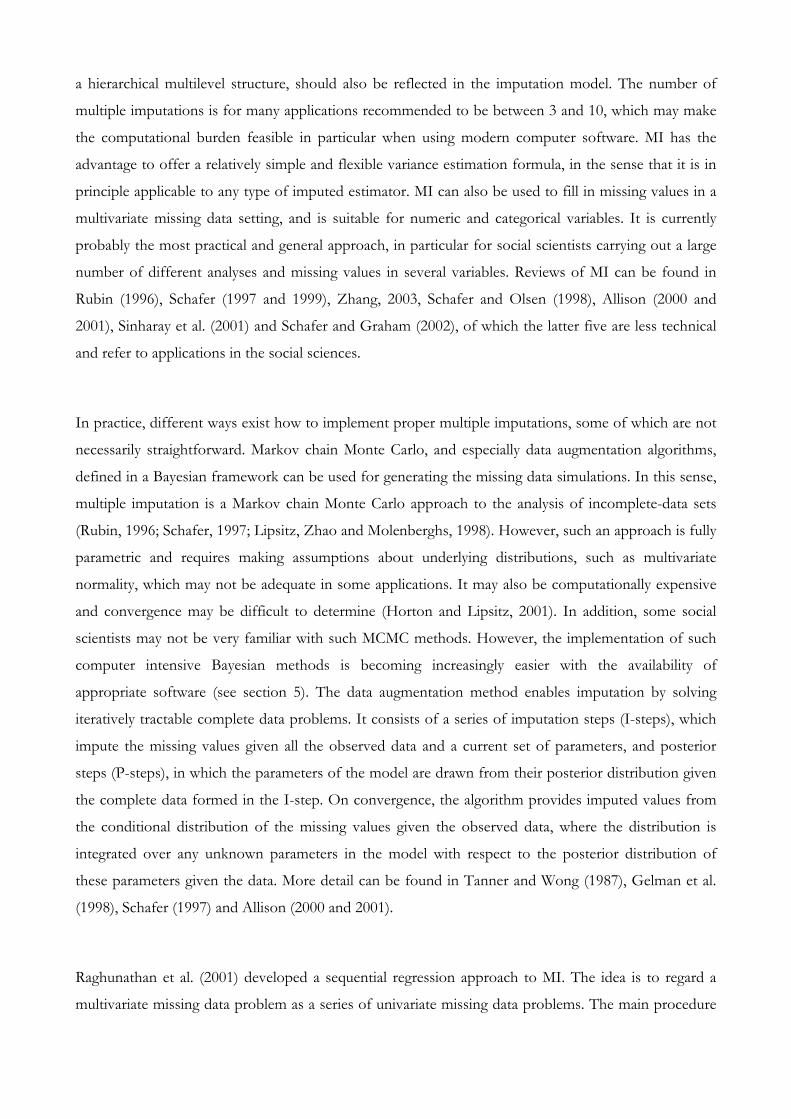
a hierarchical multilevel structure, should also be reflected in the imputation model. The number of
multiple imputations is for many applications recommended to be between 3 and 10, which may make
the computational burden feasible in particular when using modern computer software. MI has the
advantage to offer a relatively simple and flexible variance estimation formula, in the sense that it is in
principle applicable to any type of imputed estimator. MI can also be used to fill in missing values in a
multivariate missing data setting, and is suitable for numeric and categorical variables. It is currently
probably the most practical and general approach, in particular for social scientists carrying out a large
number of different analyses and missing values in several variables. Reviews of MI can be found in
Rubin (1996), Schafer (1997 and 1999), Zhang, 2003, Schafer and Olsen (1998), Allison (2000 and
2001), Sinharay et al. (2001) and Schafer and Graham (2002), of which the latter five are less technical
and refer to applications in the social sciences.
In practice, different ways exist how to implement proper multiple imputations, some of which are not
necessarily straightforward. Markov chain Monte Carlo, and especially data augmentation algorithms,
defined in a Bayesian framework can be used for generating the missing data simulations. In this sense,
multiple imputation is a Markov chain Monte Carlo approach to the analysis of incomplete-data sets
(Rubin, 1996; Schafer, 1997; Lipsitz, Zhao and Molenberghs, 1998). However, such an approach is fully
parametric and requires making assumptions about underlying distributions, such as multivariate
normality, which may not be adequate in some applications. It may also be computationally expensive
and convergence may be difficult to determine (Horton and Lipsitz, 2001). In addition, some social
scientists may not be very familiar with such MCMC methods. However, the implementation of such
computer intensive Bayesian methods is becoming increasingly easier with the availability of
appropriate software (see section 5). The data augmentation method enables imputation by solving
iteratively tractable complete data problems. It consists of a series of imputation steps (I-steps), which
impute the missing values given all the observed data and a current set of parameters, and posterior
steps (P-steps), in which the parameters of the model are drawn from their posterior distribution given
the complete data formed in the I-step. On convergence, the algorithm provides imputed values from
the conditional distribution of the missing values given the observed data, where the distribution is
integrated over any unknown parameters in the model with respect to the posterior distribution of
these parameters given the data. More detail can be found in Tanner and Wong (1987), Gelman et al.
(1998), Schafer (1997) and Allison (2000 and 2001).
Raghunathan et al. (2001) developed a sequential regression approach to MI. The idea is to regard a
multivariate missing data problem as a series of univariate missing data problems. The main procedure
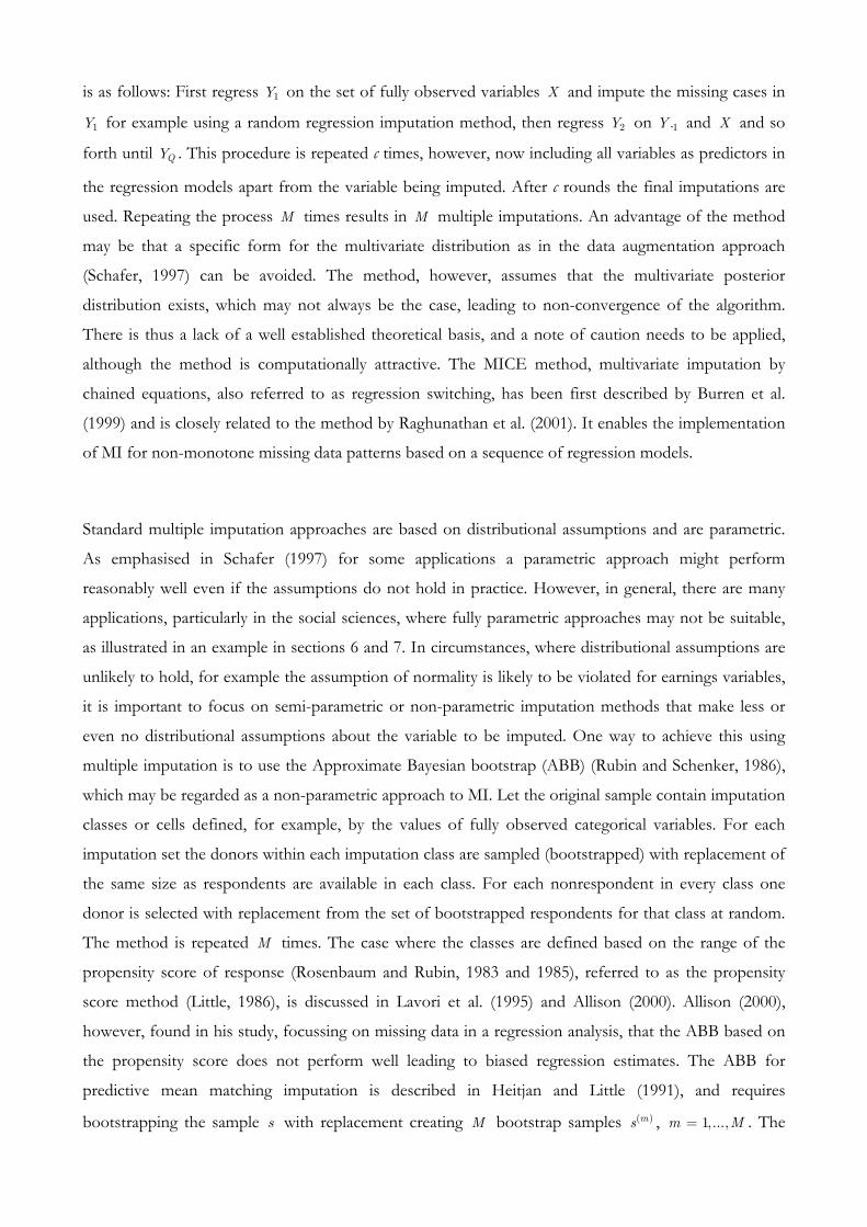
is as follows: First regress 1Y on the set of fully observed variables X and impute the missing cases in
1Y for example using a random regression imputation method, then regress 2Y on 1.Y and X and so
forth until QY . This procedure is repeated c times, however, now including all variables as predictors in
the regression models apart from the variable being imputed. After c rounds the final imputations are
used. Repeating the process M times results in M multiple imputations. An advantage of the method
may be that a specific form for the multivariate distribution as in the data augmentation approach
(Schafer, 1997) can be avoided. The method, however, assumes that the multivariate posterior
distribution exists, which may not always be the case, leading to non-convergence of the algorithm.
There is thus a lack of a well established theoretical basis, and a note of caution needs to be applied,
although the method is computationally attractive. The MICE method, multivariate imputation by
chained equations, also referred to as regression switching, has been first described by Burren et al.
(1999) and is closely related to the method by Raghunathan et al. (2001). It enables the implementation
of MI for non-monotone missing data patterns based on a sequence of regression models.
Standard multiple imputation approaches are based on distributional assumptions and are parametric.
As emphasised in Schafer (1997) for some applications a parametric approach might perform
reasonably well even if the assumptions do not hold in practice. However, in general, there are many
applications, particularly in the social sciences, where fully parametric approaches may not be suitable,
as illustrated in an example in sections 6 and 7. In circumstances, where distributional assumptions are
unlikely to hold, for example the assumption of normality is likely to be violated for earnings variables,
it is important to focus on semi-parametric or non-parametric imputation methods that make less or
even no distributional assumptions about the variable to be imputed. One way to achieve this using
multiple imputation is to use the Approximate Bayesian bootstrap (ABB) (Rubin and Schenker, 1986),
which may be regarded as a non-parametric approach to MI. Let the original sample contain imputation
classes or cells defined, for example, by the values of fully observed categorical variables. For each
imputation set the donors within each imputation class are sampled (bootstrapped) with replacement of
the same size as respondents are available in each class. For each nonrespondent in every class one
donor is selected with replacement from the set of bootstrapped respondents for that class at random.
The method is repeated M times. The case where the classes are defined based on the range of the
propensity score of response (Rosenbaum and Rubin, 1983 and 1985), referred to as the propensity
score method (Little, 1986), is discussed in Lavori et al. (1995) and Allison (2000). Allison (2000),
however, found in his study, focussing on missing data in a regression analysis, that the ABB based on
the propensity score does not perform well leading to biased regression estimates. The ABB for
predictive mean matching imputation is described in Heitjan and Little (1991), and requires
bootstrapping the sample s with replacement creating M bootstrap samples ( )ms , 1,...,m M= . The
parameters of the imputation model are estimated based on respondents only for each bootstrap
sample, to reflect parameter uncertainty, and the predicted values, ( )ˆmiy , are defined for each bootstrap
sample. Based on these values predictive mean matching imputation is performed, by drawing at
random one donor value from a set of nearest neighbours, e.g. defined as the nearest 5 above and 5
below the predicted value of ( )ˆmjy , 0jr = . Some cases, however, have been reported where the multiple
imputation variance estimation formula does not perform well when using the ABB method (Heitjan
and Little, 1991; Rao, 1996; Kim, 2002; Kim and Fuller, 2004). An alternative less parametric MI
approach is to incorporate a hot deck method in the MI data augmentation procedure as suggested in
Durrant and Skinner (2005b) and Durrant (2005) or to consider the partially parametric techniques in
Schenker and Taylor (1996). Such a combination of methods may have certain advantages such as
overcoming distributional assumptions by using a hot deck method and at the same time providing a
simple variance estimation formula by using MI.
4.6.2. Fractional Imputation
Another form of repeated imputation is the method of fractional imputation (Kalton and Kish, 1984;
Fay, 1996; Kim and Fuller, 2004; Durrant and Skinner, 2005a), which is based on the idea of repeating a
random imputation method several times. Fractional imputation views the resulting estimator as a
weighted estimator with fractional weights 1/M for each of the imputed values and the estimator .θ can
be expressed in the same way as under multiple imputation in (4). Examples of fractional imputation
are the use of repeated random hot deck and repeated predictive mean matching imputation. The main
aim of repeated imputation is to improve the efficiency of the imputed point estimator. Kim and Fuller
(2004) find in their study that fractional imputation is more efficient than multiple imputation based on
the same number of repeated imputations. This is because of the additional variability in the MI
methods, required to achieve proper MI, for example when drawing parameters from their posterior
distributions to reflect uncertainty in the parameter estimates. An advantage of fractional imputation is
that per definition the method is based on hot deck imputation, which makes less or no distributional
assumptions in comparison to a fully a parametric method, imputes actually observed values and can
preserve distributional properties of the data. This may be important when imputing categorical
variables or variables with certain distributional features. Another potential advantage of fractional
imputation is that multiple datasets may not need to be stored which could make the data handling
under fractional imputation under certain circumstances easier than under multiple imputation where
M complete data files need to be stored and analysed. Under fractional hot deck imputation it is
enough to store the replication weights, indicating how often a donor has been used for imputation, to
carry out further analysis (Kim and Fuller, 2004). Let iw denote the imputation weight for donor i ,
1ir = , then 1i iw a= + and ia is the number of times the donor i has been used for imputation. The
estimator in (4) then reduces to a weighted estimator based on iw and only fully responding units. For
example, when estimating the total of the variable iy the fractionally imputed estimator .θ may be
expressed as a weighted estimator of the form
. /i i ii r i rw y wθ
∈ ∈=∑ ∑ . (6)
Properties of such (fractionally imputed) weighted estimators are discussed in Durrant and Skinner
(2005a) and Kim and Fuller (2004). In Durrant and Skinner (2005a) it is shown that corresponding
variance estimation formulae are also based on the weights iw and only responding units, which may
be an attractive feature, simplifying data storage and analysis, at least for the univariate case.
4.7. Debate on Single, Fractional and Multiple Imputation: A Note of Caution
Recently, some misconceptions about the use and applicability of certain types of imputation methods
have been mentioned in the literature. Non-multiple approaches to imputation have been described as
‘older’ or as ‘conventional’ imputation methods and their use has been ‘discouraged’ (Schafer and
Graham, 2002; Allison, 2001). In contrast, (proper) multiple imputation methods have been promoted
and are described as ‘modern’ methods. It is often stressed in the literature that single value imputation
and so-called improper multiple imputations, including factional imputation, treat the imputed values as
known and thus do not reflect sampling variability under a model of nonresponse correctly leading to
underestimation of the variance and therefore to undercoverage (Schafer, 1999; Sinharay, Stern and
Russel, 2001; Schafer and Graham, 2002; Carlin, 2003; Raghunathan, 2004). It is emphasised that MI
addresses the uncertainty due to imputation and it is concluded that MI is superior (Sinharay, Stern and
Russel, 2001). Although variance estimation under imputation is not the emphasis in this paper, I feel,
however, that these statements need some clarification, in particular for researchers not very familiar
with nonresponse adjustment methods.
In general, all imputation methods (also proper MI) require adjustments to the standard formulae to
reflect the additional variability due to nonresponse and imputation correctly. The adjustment to the
variance estimation formula in the case of MI (see equation (5)) is simple to implement in practice
which is an advantage for practitioners and researchers without special knowledge of such statistical
adjustment methods. The term .G approximates the standard variance estimation formula for complete
data whereas ˆ(1 1/ )M B+ reflects the adjustment necessary to capture the increased variability due to
imputation and nonresponse. However, also the MI variance estimation formula may not estimate the
variance correctly depending on, for example, the point estimator of interest or the way the multiple
imputations were generated (Fay, 1996; Kim and Fuller, 2004; Nielsen, 2003; Allison, 2000). For
example, Kim and Fuller (2004) show that the MI variance estimator is seriously biased for the variance
of a domain mean with a relative bias of about 50%. They also show that MI variance estimation may
be less stable and confidence intervals may be more variable with smaller coverage rates than under
alternative fractional imputation methods. Fay (1996) also reports longer confidence intervals under
MI. Allison (2000) reports that different approaches to MI may show a quite different performance
depending on the application and context in which such methods are used. Although recommended as
a general tool, MI should not be used without careful consideration of underlying assumptions and
models to a particular application. Fay (1996) even recommends the use of a simulation study to
examine the performance of MI before applying this method to a specific problem, and this may be
advisable for all missing data adjustment methods.
It should be stressed that also under single value and fractional imputation it is possible to estimate the
variance of an imputed estimator correctly using methods as described in section 4. Kim and Fuller
(2004) suggest a consistent replication variance estimation procedure under fractional hot deck
imputation, which is independent of the specific hot deck method used. Durrant and Skinner (2005a)
discuss variance estimation under fractional nearest neighbour imputation, based on an approach
proposed by Chen and Shao (2000). Fuller and Kim (2005) develop a jackknife variance estimation
technique for fractional nearest neighbour imputation. However, since variance estimation is not the
main focus of this paper these approaches will not be discussed further. An alternative approach would
be to extend single value imputation methods to (proper) MI approaches such that the simple variance
estimation formula in (5) is valid. For example, a hot deck imputation method may be used multiple
times using the ABB or by drawing the parameters of underlying models from their posterior
distributions (Schenker and Taylor, 1996). Another approach would be to incorporate hot deck
methods in the MI data augmentation procedure as suggested in Durrant and Skinner (2005b). These
approaches show that there may not be such a clear divide between these methods as emphasised in
some of the literature, describing hot deck methods as ‘old imputation methods’ and MI methods as
‘modern methods’ (Schafer and Graham, 2002).
5. Software for Imputation
For general social science researchers, the use of imputation in practice is likely to depend on which
algorithms are available in standard computer packages. Over the last few years, however, a number of
missing data routines have been implemented in some software packages and are now available for use.
Some require the export of data into a specialised imputation software but some routines have been
implemented in software often used by social scientists. For multiple imputation a wide range of free
and commercial software has been developed in recent years which makes MI more widely applicable
to many researchers. The following gives a brief overview and update of programmes that are currently
available. All of these procedures assume MAR and are not readily available for nonignorable
nonresponse mechanisms. Since programmes such as SPSS and STATA are widely used within the
social science community their functions are described first.
The SPSS procedure Missing Value Analysis (MVA) includes a variety of techniques to analyse the
missing data pattern, including a test of MCAR based on Little (1988 Dec.). It calculates some basic
statistics of variables subject to nonresponse and handles missing data based on a listwise or pairwise
method, regression imputation or the EM (estimation – maximisation) method, a maximum-likelihood
based method, described in Schafer (1997). The regression imputation method allows for the
imputation of predicted values, or using adjustments such as adding on observed or randomly drawn
residuals from a distribution. Overall, the functions in the MVA procedure are limited. Hot deck
procedures for example are not included. In particular, SPSS does not include proper multiple
imputation procedures. Hot deck imputation within classes, nearest neighbour and predictive mean
matching imputation may be implemented in SPSS using appropriate commands from the general data
and statistics menu (e.g. by ordering the dataset and selecting donor values appropriately), but no
readily available command is implemented in the software.
Another computer package that is often used by social scientists is STATA. STATA includes options
for various forms of hot deck imputation (e.g. using the library ‘sg116’) based on the approximate
Bayesian bootstrap and regression imputation. In particular, it includes options for multiple imputation
based on the implementation of the MICE method for multiple multivariate data imputation using the
add on library ‘st0067’ (Royston, 2004). The function ‘mvis’ imputes multivariate missing data and the
function ‘uvis’ performs imputation of missing values for the univariate case. An advantage is that both
libraries can make use not just of random regression imputation but also of predictive mean matching
imputation which enables the imputation of observed values (hot deck). The analysis of multiple
imputed datasets is facilitated with the library ‘st0042’ which assumes that multiple imputation data sets
have already been generated (Carlin, et al. 2003). The function ‘micombine’ fits a wide variety of
regression models to multiply imputed datasets combining the estimates using Rubin’s rules. STATA,
however, currently does not include MI based on data augmentation algorithms which is a
disadvantage.
Packages such as Splus and R are widely used by statisticians and economists and are used more and
more by social scientists. Both facilitate the implementation of hot deck procedures, regression and
predictive mean matching imputation. Splus includes a missing data analysis library which enables
parametric model-based procedures. It facilitates the implementation of the EM algorithm and MI
based on data augmentation (MCMC) for numeric variables, assuming multivariate normality, and for
categorical and mixed variables as described in Schafer (1997). The routines are based on programmes
such as NORM, CAT and MIX, developed by Schafer (1997), which are either for the use in Splus or
as a stand-alone Windows software for multivariate normal, categorical, mixed continuous and
categorical data respectively. Parametric assumptions, such as multivariate normality, are necessary and
the implementation of hot deck methods within such MI procedures is not possible. The programme
PAN has been developed for panel data (Schafer, 2001). The missing data library includes methods for
the analysis of convergence, the analysis of multiple complete datasets and options for the analysis of
missing data patterns. (Norm, Cat, Mix and Pan are available from
http://www.stat.psu.edu/~jls/misoftwa.html). Another Splus based library is MICE, implementing MI
using a sequence of regression models. It allows for a variety of imputation models including predictive
mean matching imputation. The software is available from www.multiple-imputation.com, maintained
by the Department of Statistics of TNO prevention and Health.
The procedures PROCMI and PROCMIANALYZE are implemented in SAS to perform MI. SAS
offers three methods for creating the multiply imputed data sets. For monotone missing data patterns
either a parametric regression method assuming a multivariate normal model or the propensity score
method can be used. For arbitrary missing data patterns a Markov Chain Monte Carlo (MCMC)
method is available assuming multivariate normality. The MIANALYZE procedure combines the
multiple imputation results. The procedures PROC DETERMINISTIC and PROC DONOR have
been developed at Statistics Canada to implement deterministic and donor imputation, the latter based
on the nearest neighbour method. The SAS-based programme SEVANI, System for Estimation of
Variance due to Nonresponse and Imputation, also developed at Statistics Canada, enables variance
estimation for certain types of estimators under imputation methods such as regression and nearest
neighbour imputation (Beaumont, 2003).
The IVEware, Imputation and Variance Estimation Software, is implemented in SAS and performs
single and multiple imputations of missing values using the sequential regression imputation method
(Raghunathan et al., 2001; http://www.isr.umich.edu/src/smp/ive/). It is also available as a stand-
alone software. The implementation of MI for multilevel models has been implemented recently in
MLwiN by Carpenter and Goldstein (2005). Their method allows imputation under a hierarchical data
structure, currently available for imputing missing covariates in a multilevel model under the
assumption of normality. Further information on the software (and more generally on MI) can be
obtained from www.missingdata.org.uk.
In addition to imputation procedures implemented in commonly used statistics software there are a
number of stand-alone packages. SOLAS is a commercial programme to perform six imputation
techniques including two techniques for MI and benefits from a well designed user interface. It
incorporates mean imputation, hot deck imputation either overall or within imputation classes and
regression imputation imputing predicted values. MI can be implemented either by using parametric
regression imputation or by the propensity score method. However, it does not incorporate MCMC
methods, and requires primarily a monotone missing data pattern. After completing the imputation the
data may be exported to other software programmes or can be analysed in SOLAS. An analysis of
missing data patterns is available. SOLAS has not been developed much further recently and its options
are somewhat limited. Allison (2000) compared NORM and SOLAS indicating that under certain
conditions SOLAS does not perform well but the freely available NORM software has certain
advantages. (More information about SOLAS is available from http://www.statsol.ie/solas/solas.htm).
Other software programmes such as AMELIA, EMCOV and MISTRESS are also available for
imputation but are not discussed here for space reasons.
A detailed discussion on computer programmes for implementing imputation can be found in Horton
and Lipsitz (2001) with particular focus on MI software. More information about software for MI and
an exhaustive list of references on MI are available from http://www.multiple-imputation.com.
Another review paper on software is HOX (1999) focusing on SPSS, SOLAS and NORM. Although by
now a wide range of different software packages are available that implement different forms of
imputation, a note of caution is necessary. It is important to understand underlying assumptions of the
procedures and to ensure their suitability for the application considered. Also, some of the routines
may be implemented slightly differently in different software and may not be directly comparable
across different computer packages. A useful tool may be the menu driven SAS based system
GENESIS, which has been developed by Statistics Canada to enable simulation studies testing the
performance of imputed estimators under different assumptions (Haziza, 2002).
Using single value or fractional imputation still requires the correct estimation of the variance by using
adjustment methods such as described in section 4. These may not be readily available in the particular
software used. The implementation of fractional hot deck methods and corresponding variance
estimation techniques in readily available software routines therefore still needs further development. If
MI is implemented in the software it is often based on the method of a sequence of regression models
which currently still lacks a thorough theoretical basis. Fully parametric MI approaches (such as
NORM) may not be suitable for some applications.
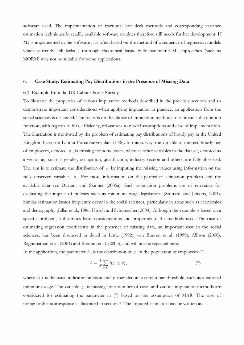
6. Case Study: Estimating Pay Distributions in the Presence of Missing Data
6.1. Example from the UK Labour Force Survey
To illustrate the properties of various imputation methods described in the previous sections and to
demonstrate important considerations when applying imputation in practice, an application from the
social sciences is discussed. The focus is on the choice of imputation methods to estimate a distribution
function, with regards to bias, efficiency, robustness to model assumptions and ease of implementation.
The illustration is motivated by the problem of estimating pay distributions of hourly pay in the United
Kingdom based on Labour Force Survey data (LFS). In this survey, the variable of interest, hourly pay
of employees, denoted iy , is missing for some cases, whereas other variables in the dataset, denoted as
a vector ix , such as gender, occupation, qualification, industry section and others, are fully observed.
The aim is to estimate the distribution of iy by imputing the missing values using information on the
fully observed variables ix . For more information on the particular estimation problem and the
available data see Durrant and Skinner (2005a). Such estimation problems are of relevance for
evaluating the impact of policies such as minimum wage legislations (Stuttard and Jenkins, 2001).
Similar estimation issues frequently occur in the social sciences, particularly in areas such as economics
and demography (Lillar et al., 1986; Hirsch and Schumacher, 2004). Although the example is based on a
specific problem, it illustrates basic considerations and properties of the methods used. The case of
estimating regression coefficients in the presence of missing data, an important case in the social
sciences, has been discussed in detail in Little (1992), van Buuren et al. (1999), Allison (2000),
Raghunathan et al. (2001) and Ibrahim et al. (2005), and will not be repeated here.
In the application, the parameter θ , is the distribution of iy in the population of employees U:
1( )i
i UI y y
Nθ
∈= ≤∑ , (7)
where (.)I is the usual indicator function and y may denote a certain pay threshold, such as a national
minimum wage. The variable iy is missing for a number of cases and various imputation methods are
considered for estimating the parameter in (7) based on the assumption of MAR. The case of
nonignorable nonresponse is illustrated in section 7. The imputed estimator may be written as
1
1. ( )n
Ii
iI y y
nθ
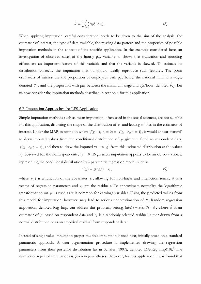
== <∑ . (8)
When applying imputation, careful consideration needs to be given to the aim of the analysis, the
estimator of interest, the type of data available, the missing data pattern and the properties of possible
imputation methods in the context of the specific application. In the example considered here, an
investigation of observed cases of the hourly pay variable iy shows that truncation and rounding
effects are an important feature of this variable and that the variable is skewed. To estimate its
distribution correctly the imputation method should ideally reproduce such features. The point
estimators of interest are the proportion of employees with pay below the national minimum wage,
denoted θ 1ˆ. , and the proportion with pay between the minimum wage and £5/hour, denoted θ 2
ˆ. . Let
us now consider the imputation methods described in section 4 for this application.
6.2. Imputation Approaches for LFS Application
Simple imputation methods such as mean imputation, often used in the social sciences, are not suitable
for this application, distorting the shape of the distribution of iy and leading to bias in the estimator of
interest. Under the MAR assumption where ( | , 0)i i if y x r = = ( | , 1)i i if y x r = , it would appear ‘natural’
to draw imputed values from the conditional distribution of y given x fitted to respondent data,
( | , 1)i i if y x r = , and then to draw the imputed values Iiy from this estimated distribution at the values
jx observed for the nonrespondents, = 0jr . Regression imputation appears to be an obvious choice,
representing the conditional distribution by a parametric regression model, such as
ln( ) ( ; )i i iy g x eβ= + , (9)
where (.)g is a function of the covariates ix , allowing for non-linear and interaction terms, β is a
vector of regression parameters and ie are the residuals. To approximate normality the logarithmic
transformation on iy is used as it is common for earnings variables. Using the predicted values from
this model for imputation, however, may lead to serious underestimation of θ . Random regression
imputation, denoted Reg Imp, can address this problem, setting ˆ ˆln( ) ( ; )Ii i iy g x eβ= + , where β is an
estimator of β based on respondent data and ie is a randomly selected residual, either drawn from a
normal distribution or as an empirical residual from respondent data.
Instead of single value imputation proper multiple imputation is used next, initially based on a standard
parametric approach. A data augmentation procedure is implemented drawing the regression
parameters from their posterior distribution (as in Schafer, 1997), denoted DA-Reg Imp(10).2 The
number of repeated imputations is given in parentheses. However, for this application it was found that
the then imputed values do not reproduce truncation and step effects of the hourly pay distribution
leading to bias around such effects. In addition, the residual assumptions made under such regression
imputation, when drawing residuals from a normal distribution with a constant variance may not hold
in this application. In particular, the assumption of a constant variance seems likely to be violated,
resulting in adding on inappropriate residuals to the predicted values (see also Schafer, 1999). This
illustrates an inadequacy of standard parametric (single or multiple) imputation approaches for this
application. The effects of such parametric approaches (Reg Imp(1) and DA-Reg Imp(10)) when
applied to LFS data can be seen in table 1, leading to quite different estimates than for the following
hot deck imputation methods, indicating an overestimation of 1θ and underestimation of 2θ . The
sensitivity towards misspecification of model assumptions for parametric methods is further illustrated
in section 7.
In contrast, hot deck imputation methods are able to relax such residual assumptions. The imputed
value from a donor will always be a genuine value and such methods seem much more suitable for this
application. The basic donor imputation method considered is predictive mean matching, based on
nearest neighbour imputation defined on the predicted values of the regression model, denoted
PMM(1). This hot deck method showed as expected a much better performance than the previous
parametric forms when applied to LFS data.
In addition to bias, it is of interest to consider the efficiency of the point estimator under imputation. A
number of approaches to reducing the variance inflation effect under nearest neighbour, due to the
multiple usage of donors, are considered. One approach is the use of a penalty function as in section 4,
discussed in Durrant and Skinner (2005a). Another possibility is to define imputation classes based on
the range of the predicted values and drawing donors by simple random sampling within classes,
denoted IC. The variance will be smaller if donors are drawn without replacement. A third approach
for reducing the variance is to employ repeated imputed values, based on fractional imputation. This is
implemented by repeating the imputation class method 10 times, denoted IC(10), ensuring that at least
10 donor values are available in each class. In addition, the predictive mean matching imputation based
on nearest neighbour is extended to fractional imputation, denoted PMM(10), by taking the 5 nearest
donor neighbours above and below the predicted value of the nonrespondent. Since these forms of
hot-deck imputation still make assumptions about the form of the imputation model these approaches
are referred to as semi-parametric methods.
The use of such forms of repeated imputation ‘naturally’ leads to the implementation of multiple
imputation taking into account the uncertainty of the parameters of the imputation model. However,
for this application clearly less parametric forms of multiple imputation need to be considered. One
possibility is to use the Approximate Bayesian Bootstrap (ABB) as in Heitjan and Little (1991) with the
aim of reflecting uncertainty of the parameter estimates by bootstrapping the LFS sample with
replacement and to estimate β in each bootstrap sample, denoted ABB-PMM(10). For comparison, the
approximate Bayesian Bootstrap method using imputation classes as suggested in Rubin and Schenker
(1986), where the classes are defined based on the predicted values, is also implemented, denoted ABB-
IC(10).
Another possibility to generate MI is to implement hot deck imputation within a data augmentation
procedure. The novelty here is to use forms of predictive mean matching within each imputation step
instead of standard regression imputation with the aim of relaxing residual assumptions, commonly
made in standard data augmentation procedures. The method is proposed by Durrant and Skinner
(2005b). The approaches implemented in the imputation step are (for more detailed technical
specifications of the algorithm see Durrant and Skinner, 2005b):
(i) Hot deck imputation within classes, denoted DA-IC(10): In each iteration, imputation classes are
defined as previously and for each nonrespondent 10 donor values are selected from the class
without replacement. Then, one donor value is selected at random from this set for imputation.
After convergence = 10M imputed sets are selected appropriately.
(ii) Nearest neighbour imputation, denoted DA-PMM(10): 10 nearest neighbours are defined as
previously and one donor value is selected at random for imputation. After convergence = 10M
imputed sets are selected appropriately.
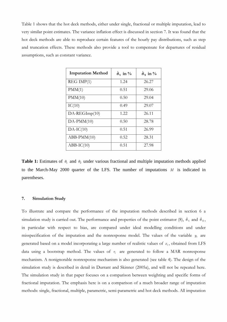
Table 1 shows that the hot deck methods, either under single, fractional or multiple imputation, lead to
very similar point estimates. The variance inflation effect is discussed in section 7. It was found that the
hot deck methods are able to reproduce certain features of the hourly pay distributions, such as step
and truncation effects. These methods also provide a tool to compensate for departures of residual
assumptions, such as constant variance.
Imputation Method 1ˆ.θ in % 2
ˆ.θ in %
REG IMP(1) 1.24 26.27
PMM(1) 0.51 29.06
PMM(10) 0.50 29.04
IC(10) 0.49 29.07
DA-REGImp(10) 1.22 26.11
DA-PMM(10) 0.50 28.78
DA-IC(10) 0.51 26.99
ABB-PMM(10) 0.52 28.31
ABB-IC(10) 0.51 27.98
Table 1: Estimates of 1θ and 2θ under various fractional and multiple imputation methods applied
to the March-May 2000 quarter of the LFS. The number of imputations M is indicated in
parentheses.
7. Simulation Study
To illustrate and compare the performance of the imputation methods described in section 6 a
simulation study is carried out. The performance and properties of the point estimator (8), 1.θ and 2.θ ,
in particular with respect to bias, are compared under ideal modelling conditions and under
misspecification of the imputation and the nonresponse model. The values of the variable iy are
generated based on a model incorporating a large number of realistic values of ix , obtained from LFS
data using a bootstrap method. The values of ir are generated to follow a MAR nonresponse
mechanism. A nonignorable nonresponse mechanism is also generated (see table 4). The design of the
simulation study is described in detail in Durrant and Skinner (2005a), and will not be repeated here.
The simulation study in that paper focuses on a comparison between weighting and specific forms of
fractional imputation. The emphasis here is on a comparison of a much broader range of imputation
methods: single, fractional, multiple, parametric, semi-parametric and hot deck methods. All imputation
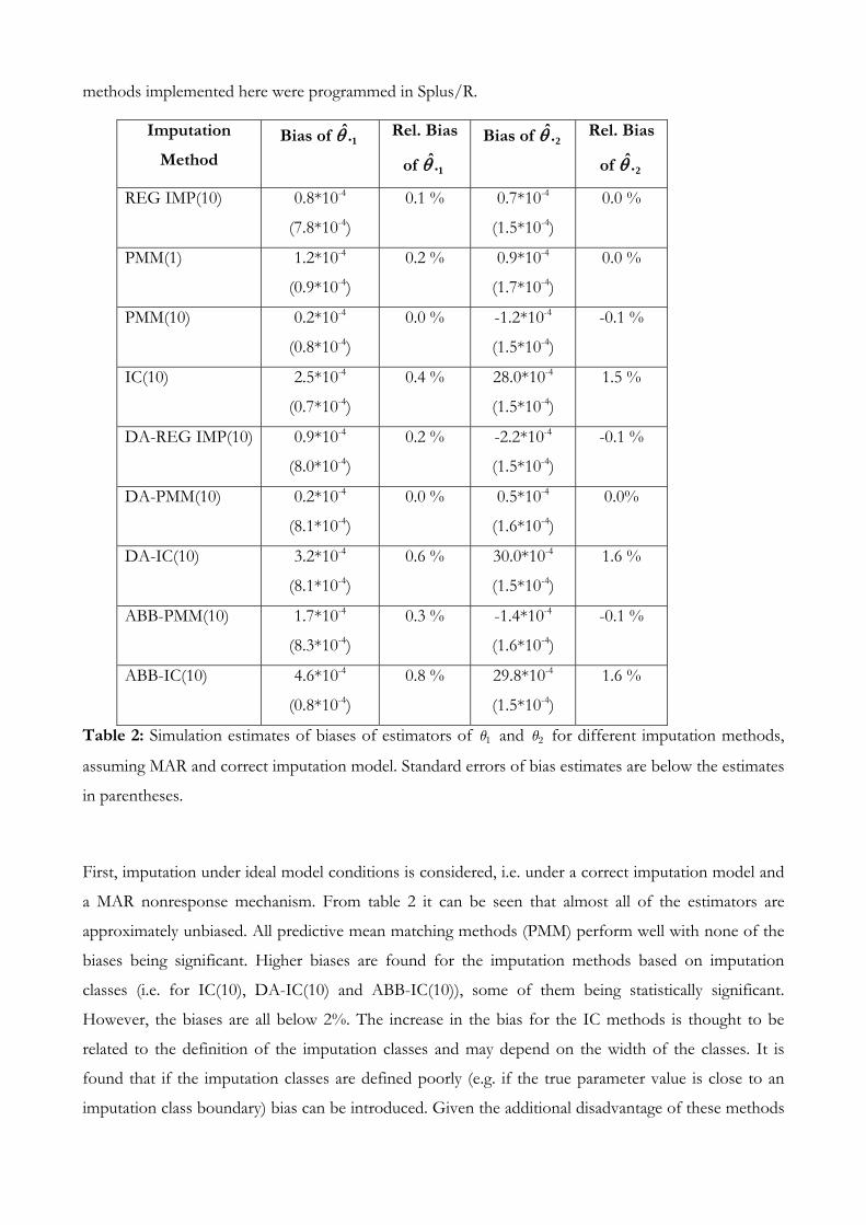
methods implemented here were programmed in Splus/R.
Imputation
Method
Bias of ˆ.1θ Rel. Bias
of ˆ.1θ
Bias of ˆ.2θ Rel. Bias
of ˆ.2θ
REG IMP(10) 0.8*10-4
(7.8*10-4)
0.1 % 0.7*10-4
(1.5*10-4)
0.0 %
PMM(1) 1.2*10-4
(0.9*10-4)
0.2 % 0.9*10-4
(1.7*10-4)
0.0 %
PMM(10) 0.2*10-4
(0.8*10-4)
0.0 % -1.2*10-4
(1.5*10-4)
-0.1 %
IC(10) 2.5*10-4
(0.7*10-4)
0.4 % 28.0*10-4
(1.5*10-4)
1.5 %
DA-REG IMP(10) 0.9*10-4
(8.0*10-4)
0.2 % -2.2*10-4
(1.5*10-4)
-0.1 %
DA-PMM(10) 0.2*10-4
(8.1*10-4)
0.0 % 0.5*10-4
(1.6*10-4)
0.0%
DA-IC(10) 3.2*10-4
(8.1*10-4)
0.6 % 30.0*10-4
(1.5*10-4)
1.6 %
ABB-PMM(10) 1.7*10-4
(8.3*10-4)
0.3 % -1.4*10-4
(1.6*10-4)
-0.1 %
ABB-IC(10) 4.6*10-4
(0.8*10-4)
0.8 % 29.8*10-4
(1.5*10-4)
1.6 %
Table 2: Simulation estimates of biases of estimators of 1θ and 2θ for different imputation methods,
assuming MAR and correct imputation model. Standard errors of bias estimates are below the estimates
in parentheses.
First, imputation under ideal model conditions is considered, i.e. under a correct imputation model and
a MAR nonresponse mechanism. From table 2 it can be seen that almost all of the estimators are
approximately unbiased. All predictive mean matching methods (PMM) perform well with none of the
biases being significant. Higher biases are found for the imputation methods based on imputation
classes (i.e. for IC(10), DA-IC(10) and ABB-IC(10)), some of them being statistically significant.
However, the biases are all below 2%. The increase in the bias for the IC methods is thought to be
related to the definition of the imputation classes and may depend on the width of the classes. It is
found that if the imputation classes are defined poorly (e.g. if the true parameter value is close to an
imputation class boundary) bias can be introduced. Given the additional disadvantage of these methods
that the definition of the boundaries of the classes are somewhat arbitrary, these methods may be
regarded as less attractive than PMM methods. Although methods based on imputation classes are
often promoted in the literature because of their simplicity (Kalton and Kasprzyk, 1986; Kim and
Fuller, 2004) and are commonly used in practice in the social sciences and in official statistics, a note of
caution should therefore be applied when using such methods. For comparison parametric methods
(i.e. REG IMP(10) and DA-REG IMP(10)) are also analysed, showing a good performance under ideal
model conditions, where residual assumptions hold approximately.
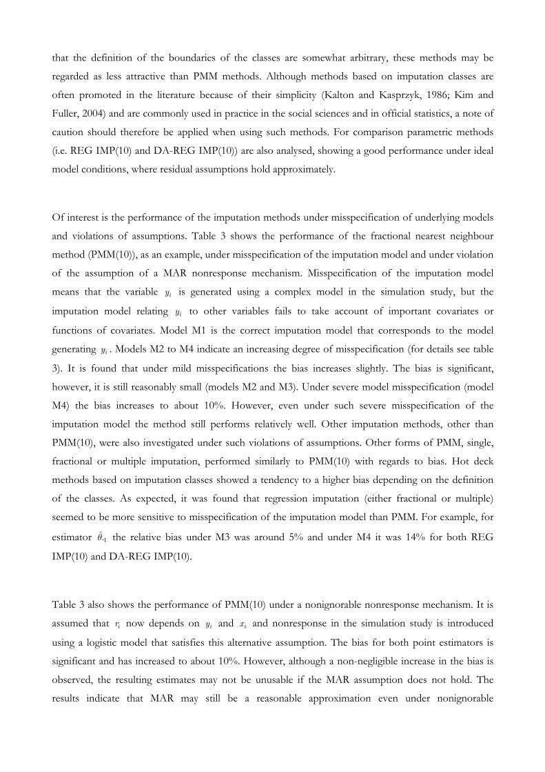
Of interest is the performance of the imputation methods under misspecification of underlying models
and violations of assumptions. Table 3 shows the performance of the fractional nearest neighbour
method (PMM(10)), as an example, under misspecification of the imputation model and under violation
of the assumption of a MAR nonresponse mechanism. Misspecification of the imputation model
means that the variable iy is generated using a complex model in the simulation study, but the
imputation model relating iy to other variables fails to take account of important covariates or
functions of covariates. Model M1 is the correct imputation model that corresponds to the model
generating iy . Models M2 to M4 indicate an increasing degree of misspecification (for details see table
3). It is found that under mild misspecifications the bias increases slightly. The bias is significant,
however, it is still reasonably small (models M2 and M3). Under severe model misspecification (model
M4) the bias increases to about 10%. However, even under such severe misspecification of the
imputation model the method still performs relatively well. Other imputation methods, other than
PMM(10), were also investigated under such violations of assumptions. Other forms of PMM, single,
fractional or multiple imputation, performed similarly to PMM(10) with regards to bias. Hot deck
methods based on imputation classes showed a tendency to a higher bias depending on the definition
of the classes. As expected, it was found that regression imputation (either fractional or multiple)
seemed to be more sensitive to misspecification of the imputation model than PMM. For example, for
estimator 1.θ the relative bias under M3 was around 5% and under M4 it was 14% for both REG
IMP(10) and DA-REG IMP(10).
Table 3 also shows the performance of PMM(10) under a nonignorable nonresponse mechanism. It is
assumed that ir now depends on iy and ix and nonresponse in the simulation study is introduced
using a logistic model that satisfies this alternative assumption. The bias for both point estimators is
significant and has increased to about 10%. However, although a non-negligible increase in the bias is
observed, the resulting estimates may not be unusable if the MAR assumption does not hold. The
results indicate that MAR may still be a reasonable approximation even under nonignorable
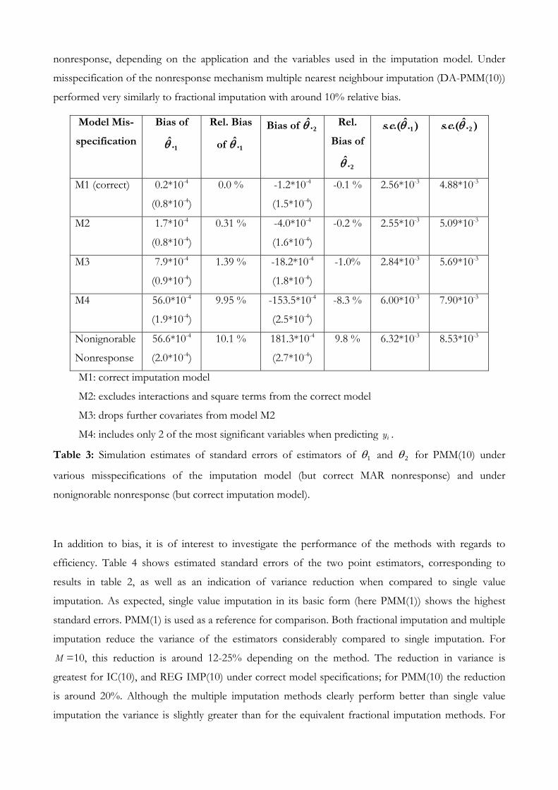
nonresponse, depending on the application and the variables used in the imputation model. Under
misspecification of the nonresponse mechanism multiple nearest neighbour imputation (DA-PMM(10))
performed very similarly to fractional imputation with around 10% relative bias.
Model Mis-
specification
Bias of
ˆ.1θ
Rel. Bias
of ˆ.1θ
Bias of ˆ.2θ Rel.
Bias of
ˆ.2θ
ˆ. .( . )1s e θ ˆ. .( . )2s e θ
M1 (correct) 0.2*10-4
(0.8*10-4)
0.0 % -1.2*10-4
(1.5*10-4)
-0.1 % 2.56*10-3 4.88*10-3
M2 1.7*10-4
(0.8*10-4)
0.31 % -4.0*10-4
(1.6*10-4)
-0.2 % 2.55*10-3 5.09*10-3
M3 7.9*10-4
(0.9*10-4)
1.39 % -18.2*10-4
(1.8*10-4)
-1.0% 2.84*10-3 5.69*10-3
M4 56.0*10-4
(1.9*10-4)
9.95 % -153.5*10-4
(2.5*10-4)
-8.3 % 6.00*10-3 7.90*10-3
Nonignorable
Nonresponse
56.6*10-4
(2.0*10-4)
10.1 % 181.3*10-4
(2.7*10-4)
9.8 % 6.32*10-3 8.53*10-3
M1: correct imputation model
M2: excludes interactions and square terms from the correct model
M3: drops further covariates from model M2
M4: includes only 2 of the most significant variables when predicting iy .
Table 3: Simulation estimates of standard errors of estimators of 1θ and 2θ for PMM(10) under
various misspecifications of the imputation model (but correct MAR nonresponse) and under
nonignorable nonresponse (but correct imputation model).
In addition to bias, it is of interest to investigate the performance of the methods with regards to
efficiency. Table 4 shows estimated standard errors of the two point estimators, corresponding to
results in table 2, as well as an indication of variance reduction when compared to single value
imputation. As expected, single value imputation in its basic form (here PMM(1)) shows the highest
standard errors. PMM(1) is used as a reference for comparison. Both fractional imputation and multiple
imputation reduce the variance of the estimators considerably compared to single imputation. For
M =10, this reduction is around 12-25% depending on the method. The reduction in variance is
greatest for IC(10), and REG IMP(10) under correct model specifications; for PMM(10) the reduction
is around 20%. Although the multiple imputation methods clearly perform better than single value
imputation the variance is slightly greater than for the equivalent fractional imputation methods. For
example, for 1.θ under PMM(10) the variance reduction is 0.83, under DA-PMM(10) it is 0.85 and
under ABB-PMM(10) it is 0.87. for IC(10) it is 0.78, for DA-IC(10) it is 0.83 and ABB-IC(10) it is 0.88,
indicating a greater efficiency for fractional imputation in comparison to MI. The effect is found to be
relatively small for small or moderate nonresponse rates. Further investigation showed that for higher
nonresponse rates (e.g. between 30% to 50%) the difference in efficiency is larger. The simulation
variance under the ABB methods was in comparison to fractional imputation about 12% larger. This
coincides with findings in Kim and Fuller (2004). Their study indicated that MI can be considerably less
efficient than fractional imputation.
It is concluded that predictive mean matching based on fractional imputation (PMM(10)) and multiple
imputation (DA-PMM(10)) seem to be the most promising approaches, relaxing the parametric
assumptions in regression imputation (REG IMP(10)), including standard parametric multiple
imputation (DA-REG IMP(10)), avoiding the potential bias of the imputation class methods (IC(10),
DA-IC(10), ABB-IC(10)) and showing appreciable efficiency gains with respect to single imputation
methods.
Imputation
Method
ˆ. .( )s e θ1 ˆ. .( )s e θ2 ˆ( )ˆ( )NN
VV
θθ1
1 1
ˆ( )
ˆ( )NN
VV
θθ2
1 2
REG IMP(10) 2.48*10-3 4.72*10-3 0.79 0.75
PMM(1) 2.79*10-3 5.43*10-3 1 1
PMM(10) 2.56*10-3 4.88*10-3 0.83 0.81
IC(10) 2.48*10-3 4.72*10-3 0.78 0.76
DA-REG IMP(10) 2.54*10-3 4.83*10-3 0.82 0.79
DA-PMM(10) 2.58*10-3 4.92*10-3 0.85 0.82
DA-IC(10) 2.55*10-3 4.86*10-3 0.83 0.80
ABB-PMM(10) 2.61*10-3 4.90*10-3 0.87 0.81
ABB-IC(10) 2.63*10-3 4.87*10-3 0.88 0.80
Table 4: Simulation estimates of standard errors of estimators of 1θ and 2θ for different imputation
methods, assuming MAR and correct imputation model.
8. Conclusions
This paper discusses a range of imputation methods to compensate for item-nonresponse in social
science data and illustrates advantages and disadvantages of the methods. It aims to clarify some
recent misconceptions and to highlight some new developments in this field. When applying
imputation it is important to consider the type of analysis and the type of point estimator of interest.
In particular, it should be distinguished if the goal is to produce unbiased and efficient estimates of
means, totals, proportions and official aggregated statistics or a complete micro-data file that can be
used for a variety of different analyses and by different users. Multiple imputation is an important
and powerful form of imputation and has the advantage that variance estimation under imputation
can be carried out comparatively easily. Fractional hot deck imputation is introduced with the aim
of improving the efficiency and the sensitivity to model misspecifications of an imputed estimator.
Based on an example from the social sciences the paper illustrates how to choose between different
methods in practice. Parametric regression imputation, including standard multiple imputation, do
not seem appropriate for situations where parametric assumptions are likely to be violated. Hot deck
methods, however, are shown to better preserve distributional properties, which is important for
many applications in the social sciences. Forms of predictive mean matching imputation perform
well even under misspecification of assumptions. To take advantage of multiple imputation and hot-
deck properties semi-parametric forms of MI, such as the incorporation of hot deck within the
imputation step of a data augmentation procedure, are proposed. In the application considered here,
fractional and multiple predictive mean matching methods seem to be the most promising
approaches with the fractional methods showing slight efficiency gains in comparison to multiple
imputation. However, further research is needed to develop semi- and non-parametric methods and
methods under nonignorable nonresponse and to make such methods easily applicable by social
scientists.
References
[1] Allison, P.D. (2000): Multiple Imputation for Missing Data, A Cautionary Tale, Sociological Methods
and Research, 28, 3, 301-309.
[2] Allison, P.D. (2001): Missing Data, Sage University Papers Series on Quantitative Applications in the Social
Sciences, series no. 07-136, Thousand Oaks.
[3] Beaumont, J.F. (2003): The System for Estimation of Variance due to Nonresponse and
Imputation (SEVANI), The Imputation Bulletin, 3,1, 2003, 6-9.
[4] Binder, D.A. and Sun, W. (1996): Frequency Valid Multiple Imputation for Surveys with a
Complex Design, Proceedings of the Section on Survey Research Methods, American Statistical Association,
281-286.
[5] Burren, v. S., Boshuizen, H.C. and Knock, D.L. (1999): Multiple Imputation of Missing Blood
Pressure Covariates in Survival Analysis, Statistics in Medicine, 18, 681-696.
[6] Carlin, J. B., Li, N., Greenwood, P. and Coffey, C. (2003): Tools for Analyzing Multiple Imputed
Datasets, The Stata Journal, 3, 3, 226-244.
[7] Carpenter, J. and Goldstein, H. (2005): Multiple Imputation in MlwiN, available from
www.missingdata.org.uk.
[8] Chambers, R. (2003): Evaluation Criteria for Statistical Editing and Imputation, National Statistical
Methodological Series, 28, Office for National Statistics, London.
[9] Chen, J. and Shao, J. (2000): Nearest Neighbour Imputation for Survey Data, Journal of Official
Statistics, 16, 2, 113-131.
[10] Chen, J. and Shao, J. (2001): Jackknife Variance Estimation for Nearest Neighbour Imputation,
Journal of the American Statistical Association, 96, 453, 260-269.
[11] David, M. H., Little, R., Samuhel, M. and Triest, R. (1983): Imputation Models based on the
Propensity to Respond, Proceedings of the Business and Economic Statistics Section, American Statistical
Association, 168-173.
[12] Deville, J.C. and Särndal, C.E. (1994): Variance Estimation for the Regression Imputed Horvitz-
Thompson Estimator, Journal of Official Statistics, 10, 4, 381-394.
[13] Durrant, G.B. (2005): A Semi-Parametric Multiple Imputation Data Augmentation Pro-cedure,
Proceedings of the Section on Survey Research Methods, American Statistical Association, forthcoming.
[14] Durrant, G.B. and Skinner, C. (2005a): Using Missing Data Methods to Correct for Measurement
Error in a Distribution Function, Survey Methodology, forthcoming.
[15] Durrant, G.B. and Skinner, C. (2005b): Using Data Augmentation to Correct for Nonignorable
Nonresponse when Surrogate Data are Available: An Application to the Distribution of Hourly
Pay, Journal of the Royal Statistical Society, Series A, forthcoming.
[16] Fay, R.E. (1996): Alternative Paradigms for the Analysis of Imputed Survey Data, Journal of the
American Statistical Association, 91, 434, 490-498.
[17] Freedman, V.A. and Wolf, D.A. (1995): A Case Study on the Use of Multiple Imputation,
Demography, 32, 3, 459-470.
[18] Fuller, W. and Kim, J.K. (2005): Replicated Nearest Neighbour Imputation, Bulletin of the
International Statistical Institute, 55th Session, Sydney.
[19] Gelman, A., Carlin, J.B., Stern, H.S. and Rubin, D.B. (1998): Bayesian Data Analysis, London.
[20] Government Statistical Service (GSS) (1996): Report of the Task Force on Imputation, Government
Statistical Service Methodology Series, 3, London.
[21] Haziza, D. (2002): Genesis, Generalised System for Imputation Simulation, The Imputation Bulletin,
2, 2, 8-10.
[22] Heitjan, D.F. (1994): Ignorability in General Incomplete-Data Models, Biometrika, 81, 4, 701-708.
[23] Heitjan, D.F. and Landis, J.R. (1994): Assessing Secular Trends in Blood Pressure, A Multiple
Imputation Approach, Journal of the American Statistical Association, 89, 427, 750-759.
[24] Heitjan, D.F. and Little, R. (1991): Multiple Imputation for the Fatal Accident Reporting System,
Journal of the Royal Statistical Society, Applied Statistics, 40, 1, 13-29.
[25] Heitjan, D.F. and Rubin, D.B. (1990): Inference from Coarse Data via Multiple Imputation with
Application to Age Heaping, Journal of the American Statistical Association, 85, 410, 304-314.
[26] Hirsch, B.T. and Schumacher, E.J. (2004): Match Bias in Wage Gap Estimates Due to Earnings
Imputation, Journal of Labour Economics, 22, 3, 689-721.
[27] Horton, N.J. and Lipsitz, S.R. (2001): Multiple Imputation in Practice: Comparison of Software
Packages for Regression Models With Missing Variables, The American Statistician, 55, 3, 244-254.
[28] HOX, J.J. (1999): A Review of Current Software for Handling Missing Data, Kwantitatieve
Methoden, 62, 123-138.
[29] Ibrahim, J.G., Chen, M.H. Lipsitz, S.R. and Herring, A.H. (2005): Missing-Data Methods for
Generalised Linear Models: A Comparative Review, Journal of the American Statistical Association,
100, 469, 332-346.
[30] Jinn, J.H. and Sedransk, J. (1989): Effect on Secondary Data Analysis of Common Imputation
Methods, Sociological Methodology, 19, 213-241.
[31] Kalton, G. (1983): Compensating for Missing Survey Data, Michigan.
[32] Kalton, G. and Kasprzyk, D. (1982): Imputing for Missing Survey Responses, Proceedings of the
Section on Survey Research Methods, American Statistical Association, 22-31.
[33] Kalton, G. and Kish, L. (1984): Some Efficient Random Imputation Methods, Communications in
Statistics, Part A, Theory and Methods, 13, 1919-1939.
[34] Kim, J.K. (2002): A Note on Approximate Bayesian Bootstrap Imputation, Biometrika, 89, 2, 470-
477.
[35] Kim, J.K. and Fuller, W. (2004): Fractional Hot Deck Imputation, Biometrika, 91, 3, 559-578.
[36] Lessler, J.T. and Kalsbeek W.D. (1992): Nonsampling Error in Surveys, New York, Chichester.
[37] Lillar, L., Smith, J.P. and Welch, F. (1986): What do We Really Know About Wages?, The
Importance of Nonreporting and Census Imputation, Journal of Political Economy, 94, 3, 489-506.
[38] Lipsitz, S.R., Zhao, L.P. and Molenberghs, G. (1998): A Semiparametric Method of Multiple
Imputation, Journal of the Royal Statistical Society, Series B, Statistical Methodology, 60, 1, 127-144.
[39] Little, R.J.A. (1986): Survey Nonresponse Adjustments for Estimates of Means, International
Statistical Review, 54, 2, 139-157.
[40] Little, R.J.A. (1988, Dec.): A Test of Missing Completely at Random for Multivariate Data with
Missing Values, Journal of the American Statistical Association, 83, 404, 1198-1202.
[41] Little, R.J.A. (1988, July): Missing-Data Adjustments in Large Surveys, Journal of Business and
Economic Statistics, 6, 3, 287-301.
[42] Little, R.J.A. and Rubin, D.B. (1990): The Analysis of Social Science Data with Missing Values,
Sociological Methods and Research, 18, 3, 292-326.
[43] Little, R.J.A. and Rubin, D.B. (2002): Statistical Analysis with Missing Data, New York.
[44] Manski, C. (1995): Identification Problems in the Social Sciences, Cambridge.
[45] Manski, C. (2005): Partial Identification with Missing Data: Concepts and Findings, International
Journal of Approximate Reasoning, 39, 2-3, 151-165.
[46] Nielsen, S.F. (2003): Proper and Improper Multiple Imputation, International Statistical Review, 71,
3, 593-627.
[47] Nordholt, E.S. (1998): Imputation: Methods, Simulation, Experiments and Practical Examples,
International Statistical Review, 66, 2, 157-180.
[48] Raghunathan, T.E., Lepkowski, J.M. van Hoewyk M., Solenberger P.W. (2001): A Multivariate
Technique for Multiply Imputing Missing Values using a Sequence of Regression Models, Survey
Methodology, 27, 85-95.
[49] Rancourt, E. (1999): Estimation with Nearest Neighbour Imputation at Statistics Canada, in:
Proceedings of the Section on Survey Research Methods, American Statistical Association, 131-138.
[50] Rao, J.N.K. (1996): On Variance Estimation with Imputed Survey Data, Journal of the American
Statistical Association, 91, 434, 499-506
[51] Rao, J.N.K. and Shao, J. (1992): Jackknife Variance Estimation with Survey Data under Hot Deck
Imputation, Biometrika, 79, 4, 811-822.
[52] Rao, J.N.K. and Sitter, R.R. (1995): Variance Estimation under Two-Phase Sampling with
Applications to Imputation for Missing Data, Biometrika, 82, 2, 453-460.
[53] Rao, J.N.K., Shao J. (1999): Modified Balanced Repeated Replication for Complex Survey Data,
Biometrika, 86, 2, 403-415.
[54] Robins, J.M. and Rotnitzky, A. (1995): Semiparametric Efficiency in Multivariate Regression
Models with Missing Data, Journal of the American Statistical Association, 90, 429, 122-129.
[55] Robins, J.M., Rotnitzky, A. and Zhao, L.P. (1994): Estimation of Regression Coefficients when
some Regressors are not Always Observed, Journal of the American Statistical Association, 89, 427,
846-866.
[56] Rosenbaum, P.R. and Rubin, D.B. (1983): The Central Role of the Propensity Score in
Observational Studies for Causal Effects, Biometrika, 70, 1, 41-55.
[57] Rosenbaum, P.R. and Rubin, D.B. (1985): Constructing a Control-Group Using Mutlivariate
Matched Sampling Methods that Incorporate the Propensity Score, The American Statistician, 39, 1,
33-38.
[58] Royston, P. (2004): Multiple Imputation of Missing Values, The Stata Journal, 4, 3, 227-241.
[59] Rubin, D.B. (1987): Multiple Imputation for Nonresponse in Surveys, New York, Chichester.
[60] Rubin, D.B. (1996): Multiple Imputation after 18+ Years, Journal of the American Statistical
Association, 91, 434, 473-489.
[61] Rubin, D.B. and Schenker. N. (1986): Multiple Imputation for Interval Estimation from Simple
Random Samples With Ignorable Nonresponse, Journal of the American Statistical Association, 81,
394, 366-374.
[62] Särndal, C.E., Swensson, B. and Wretman, J. (1992): Model Assisted Survey Sampling, New York.
[63] Schafer J.L. (1999): Multiple Imputation: A Primer, Statistical Methods in Medical Research, 8, 3-15.
[64] Schafer, J. L. (1997): Analysis of Incomplete Multivariate Data, London.
[65] Schafer, J.L. (1999): Multiple Imputation: A Primer, Statistical Methods in Medical Research, 8, 3-
15.
[66] Schafer, J.L. (2001): Multiple Imputation with Pan, in: Collins, L.M. and Sayer, A.G. (eds), New
Methods for the Analysis of Change, Washington, 2001, 357-377.
[67] Schafer, J.L. and Graham, J.W. (2002): Missing Data: Our View of the State of the Art,
Psychological Methods,7, 2, 147-177.
[68] Schafer, J.L. and Olsen,M.K. (1998): Multiple Imputation for Multivariate Missing-Data
Problems: A Data Analyst’s Perspective, Multivariate Behavioral Research, 33, 545-571.
[69] Schenker, N. and Taylor, J.M.G. (1996): Partially Parametric Techniques for Multiple Imputation,
Computational Statistics and Data Analysis, 22, 425-446.
[70] Shao, J and Sitter, R.R. (1996): Bootstrap for Imputed Survey Data, Journal of the American Statistical
Association, Theory and Methods, 91, 435, 1278-1286.
[71] Shao, J. and Steel, P. (1999): Variance Estimation for Survey Data with Composite Imputation
and Nonnegligible Sampling Fractions, Journal of the American Statistical Association, Theory and
Methods, 94, 445, 254-265.
[72] Sinharay, S., Stern, H.S. and Russell, D. (2001): The Use of Multiple Imputation for the Analysis
of Missing Data, Psychological Methods, 6, 317-329.
[73] Skinner, C. and Rao, J.N.K. (2002): Jackknife Variance Estimation for Multivariate Statistics

under Hot Deck Imputation From Common Donors, Journal of Statistical Planning and Inference, 102,
1, 421-422.
[74] Stuttard, N. and Jenkins, J. (2001): Measuring Low Pay Using the New Earnings Survey and the
Labour Force Survey, Labour Market Trends, 55-66.
[75] Tanner, M.A. and Wong, W.H. (1987): The Calculation of Posterior Distributions by Data
Augmentation, Journal of the American Statistical Association, 82, 398, 528-540.
[76] Yung, W. and Rao, J.N.K. (2000): Jackknife variance estimation under imputation for estimators
using poststratification information, Journal of the American Statistical Association, 95, 451, 903-915.
[77] Zhang, P. (2003): Multiple Imputation: Theory and Method, International Statistical Review, 71, 3,
581-592 (with discussions).


![[MI] Multiple Imputation - Stata](https://img.pdfslide.net/doc/110x75/62039c6dda24ad121e4b6a82/mi-multiple-imputation-stata.jpg)