Embed Size (px)
Citation preview

Research Collection
Doctoral Thesis
Unique sink orientations of cubes
Author(s): Schurr, Ingo A.
Publication Date: 2004
Permanent Link: https://doi.org/10.3929/ethz-a-004844278
Rights / License: In Copyright - Non-Commercial Use Permitted
This page was generated automatically upon download from the ETH Zurich Research Collection. For moreinformation please consult the Terms of use.
ETH Library
DISS. ETH NO. 15747
Unique Sink Orientations of Cubes
A dissertation submitted to the
Swiss Federal Institute of Technology Zürich
for the degree of Doctor of Sciences
presented by
Ingo Andreas Schurr
Dipl. Math., Freie Universität Berlin, Germanyborn March 12, 1972 in Baden-Baden, Germany
citizen of Germany
accepted on the recomodation of
Prof. Dr. Emo Welzl, ETH Zürich, examiner
Dr. Tibor Szabo, ETH Zürich, co-examiner
Prof. Günter Ziegler, TU Berlin, co-examiner


Acknowledgments
I would like to express my deep gratitude to my advisor Emo Welzl. His
idea of a Pre-Doc program gave me the chance to sneak into the world
of discrete mathematics. Furthermore, all I know about how science
works, I know from him.
I am also deeply grateful for being the first Ph.D. student of Tibor
Szabo. He was a wonderful advisor. Thanks for reading and commenting
(nearly) every single page of this thesis.
Thanks to Günter Ziegler, not only for being my third supervisor, but
also for letting me stay in his group in Berlin for one semester.
Without Bernd Gärtner a whole chapter of this thesis would never
have been written. Thanks for all the fruitful discussions about linear
programing and the business class.
I would like to thank Andrea Hoffkamp (for all the "germanisms"and the (soap) operas), Arnold Wassmer (for sharing his mathematical
thoughts with me), Carsten Lange (for sharing his experience), Enno
Brehm (for all I know about programming), Falk Tschirschnitz (forproofreading), Iris Klick (for at least trying to read), Kaspar Fischer
(for all his advices and the roar of the tiger), Mark de Longueville (forteaching me Analysis and all the comments), Nando Cicalese (for the
espresso and last minute words of wisdom), Shankar Ram Lakshmi-
narayanan (for sharing a flat and all the questions and answers), Uli
Wagner (for forcing me into the pre-doc program, sharing a flat and
enlightening me) and Zsuzsa (for bringing me to Zürich, sharing a flat
and criticizing my criticisms). Without you I would not have been able
to finish this thesis.
Thanks to the first pre-docs Frank Vallentin, Godfrey Njulumi Justo,
Hiroyuki Miyazawa, Sai Anand, and Stamatis Stefanakos. It was a great
half-a-year.
Last, but not least, I am very thankful for being part of the gremo
group. Thank you all, it was a pleasure working with you.
m

Abstract
Subject of this thesis is the theory of unique sink orientations of cubes.
Such orientations are suitable to model problems from different areas of
combinatorial optimization. In particular, unique sink orientations are
closely related to the running time of the simplex algorithm.In the following, we try to answer three main questions: How can
optimization problems be translated into the framework of unique sink
orientations? What structural properties do unique sink orientations
have? And how difficult is the algorithmic problem of finding the sink
of a unique sink orientation?
In connection to the first question, the main result is a reduction from
linear programming to unique sink orientations. Although the connec¬
tion to linear programming was the core motivation for our studies, it
was not clear in the beginning how general linear programs can be fit
into the theory of unique sink orientations. The reduction presented in
this thesis closes this gap.
For the second question we can provide several construction schemes
for unique sink orientations. On the one hand we know schemes which
allow us to construct all unique sink orientations. On the other hand we
present easier constructions, which are still powerful enough to provideus with a number of interesting orientations. The hope that unique sink
orientations on their own carry an interesting algebraic structure turns
out to be wrong.
Equipped with the construction schemes just mentioned we are able
to give some answers to the third question about the algorithmic com¬
plexity. The true complexity of the problem of finding a sink of a uniquesink orientation remains open. But we can provide first lower bounds
for special algorithms as well as for the general case. Furthermore, it
turns out that the algorithmic problem is NP-hard only if NP=coNP.
IV
Zusammenfassung
Gegenstand der vorliegenden Arbeit sind Orientierungen des Kanten-
Graphs eines Hyperwürfels, so dass jeder Unterwürfel eine eindeutigeSenke hat (im folgenden ESE-Würfel genannt). Solche Orientierungenmodellieren etliche Probleme aus unterschiedlichen Bereichen der kom¬
binatorischen Optimierung. Insbesondere besteht ein enger Zusammen¬
hang zu der (seit langem) offenen Frage nach der Laufzeit des Simpex-
Algorithmus.Im folgenden werden im Wesentlichen drei Themenkomplexe behan¬
delt: Wie können Optimierungs-Probleme auf ESE-Würfel reduziert
werden? Welche strukturellen Aussagen kann man über ESE-Würfel
machen? Und wie schwer ist das algorithmische Problem, die Senke
eines ESE-Würfels zu finden?
Im Zusammenhang mit der ersten Frage ist die Reduktion von line¬
arem Programmieren auf ESE-Würfel hervorzuheben. Die Verbindungzwischen linearem Programmieren und ESE-Würfeln war zwar von An¬
fang an Motivation für die vorliegenden Studien, lange Zeit jedoch war
es nicht klar, wie allgemeine lineare Programme in die Theorie der ESE-
Würfel passen. Die hier vorgestellte Reduktion schliesst diese Lücke.
Bezüglich der zweien Frage sind vor allem eine Reihe von Konstruk¬
tionsvorschriften für ESE-Würfel zu nennen. Auf der einen Seite haben
wir ein allgemeines Konstruktions-Schema, das stark genug ist, alle ESE-
Würfel zu generieren, auf der anderen Seite stellen wir einige deutlich
einfachere Konstruktionen vor, die allerdings noch mächtig genug sind,um interessante ESE-Würfel zu beschreiben.
Mit Hilfe dieser Konstruktionsvorschriften ist es uns möglich, auch
Antworten auf die dritte Frage nach der algorithmischen Komplexitätzu finden. Zwar ist die wirkliche Komplexität des Problems die Senke
zu finden weiterhin offen, aber es ist uns möglich, untere Schranken
herzuleiten, sowohl für spezielle Algorithmen, als auch für den allge¬meinen Fall. Des weiteren wird gezeigt, dass das algorithmische Problem
nur dann NP-schwer sein kann, wenn NP=coNP gilt.
v

vi

Contents
1 Motivation 1
1.1 Linear Programming 2
1.2 The Object of Interest 4
1.3 Outline of the Thesis 5
1.4 Remarks on the Notation 6
2 Basics 9
2.1 The Cube 10
2.2 Unique Sinks 13
2.3 Complexity Issues 18
2.4 Remarks 21
3 Sources 23
3.1 Linear Programming 24
3.2 Linear Complementarity Problems 28
3.3 Strong LP-type Problems 31
3.4 Strictly Convex (Quadratic) Programming 40
3.5 Linear Programming Revisited 47
3.6 Remarks 59
4 Structure 61
4.1 Outmaps 62
4.2 Algebraic Excursion 66
4.3 Phases 69
4.4 Local Changes 81
4.5 Products 84
4.6 Examples 88
4.6.1 Partial Unique Sink Orientations 88
4.6.2 Combed and Decomposable Orientations....
93
4.6.3 Klee-Minty Cubes 93
vii

Contents
4.6.4 Matching Flip Orientations 96
4.7 Remarks 99
5 Algorithms 101
5.1 Complexity Model 102
5.2 A Lower Bound on Deterministic Algorithms 105
5.3 Small Dimensions 108
5.4 Fast Subclasses 122
5.5 Jump Antipodal 124
5.6 Remarks 131
6 Data 133
6.1 Storing Orientations 134
6.2 Implementational Aspects 141
6.2.1 Isomorphism Test 141
6.2.2 Enumeration 145
6.3 Dimension 3 149
6.4 Dimension 4 151
6.5 Dimension 5 and higher 153
Bibliography 158
Curriculum Vitae 162
vm

1 Motivation
It's a very funny thought
that, if Bears were Bees,
They'd build their nests at
the bottom of trees And
that being so (if the Bees
were Bears), We shouldn't
have to climb up all these
stairs
(Winnie The Pooh)
1

1 Motivation
1.1 Linear Programming
Back in the 1940, the term "program" (as military term) referred to a
plan or schedule for training, logistical supply or deployment of men
To automatize such programming, the young mathematician George
Dantzig introduced a mathematical model for programrmng in a linear-
structure He first presented his idea to a broader audience in 1948 at a
meeting of the Econometric Society in Wisconsin In [7] Dantzig writes
about this meeting
After my talk, the chairman called for discussion For a
moment there was the usual dead silence, then a hand was
raised It was Hotelhng's I must hasten to explain that
Hotelhng was fat He used to love to swim m the ocean and
when he did, it is said that the level of the ocean rose per¬
ceptibly This huge whale of a man stood up m the back of
the room, his expressive fat face took on one of those all-
knowing smiles we all know so well He said 'But we all
know the world is nonlinear '
Having uttered this devastat¬
ing criticism of my model, he majestically sat down And
there I was, a virtual unknown, frantically trying to compose
a proper reply
Even worse, the algorithm Dantzig introduced to solve such linear pro¬
grams used a discrete structure only A linear functional on a polytopeattains its maximum in a vertex Therefore, one can find such a max¬
imal vertex by following ascending edges from vertex to vertex This
so-called simplex method only uses the edge graph of a polytope, a
discrete object Although the world is not discrete, linear programming
and the simplex method proved to be very powerful tool to solve real-life
optimization problems
Despite its usefulness in practice, the simplex method is bad in the¬
ory In 1972, Klee and Minty [24] constructed examples on which the
simplex algorithm using Dantzig's pivot rule visits all vertices Based on
their example, similar worst case behavior can be attained for nearly all
deterministic pivot rules (see [3] for a general construction scheme) It
took another eight years before Khachiyan [23] developed an algorithmfor linear programming which has polynomial running time in the bit-
2
1 1 Linear Programming
model That is, given the linear constraints of a linear program encoded
in a bit-sequence, Khachiyan's algorithm has a running time polynomialin the number of bits
From the point of view of the simplex method, this bit-model is not
satisfactory As mentioned earlier, the simplex method employs a rather
combinatorial structure of linear programming In particular, perturb¬
ing the linear program (1 e,the defining hyperplanes) slightly does not
change its combinatorics But such perturbation can drastically changethe size of its encoding
This observation leads to the attempt to find algorithms which are
polynomial in the combinatorial complexity of a linear program, which
is given by the number of linear constraints of the underlying polytopeand its dimension So far, no such algorithm is known nor are there
arguments indicating that the problem cannot be solved in polynomialtime
The best known result is achieved by RandomFacet, a random¬
ized algorithm independently developed by Kalai [21] and Matousek,
Sharir, and Welzl [28] RandomFacet is linear in the number of con¬
straints and subexponential in the dimension Remarkably, Random-
Facet works in a much more general setting than the original problemof solving a linear program
Following the approach of Kalai, RandomFacet maximizes an ab¬
stract objective function Such a function assigns values to the vertices
of the edge graph of a polytope such that every face has a unique maxi¬
mal vertex A further abstraction from the values yields an orientation
of the edge graph by orienting edges towards the vertex with highervalue Since every face has a maximal vertex v, this vertex is a sink,l e
, every edge incident to v is oriented towards v1 Such an orientation
is called unique sink orientation
The focus of this thesis is on unique sink orientations of cubes That
is, we study orientations on the edge graph of a cube such that ev¬
ery subcube has a unique sink 2 In particular, an abstract objectivefunction on a cube induces a unique sink orientation Although linear
programming was the motivating example for us to study unique sink
1See Section 3 1
2 See Chapter 2
3

1 Motivation
orientations of cubes, the concept originates from a different source In
1978, Stickney and Watson [40] introduced such orientations to studycertain linear complementarity problems
3 In this set-up the cube is
best viewed as a Boolean lattice rather than as a geometric objectThe mam advantage of unique sink orientations of cubes over general
unique sink orientations (on polytopes) lies in the additional structure
of the cube In particular, in a cube every vertex can be addressed
directly This permits formulating algorithms other than the simplexmethod For instance, the fastest known deterministic sink-finding al¬
gorithm FiBONACClSEESAW [42] maintains a data structure consisting
of two antipodal subcubes and jumps between these two subcubes
1.2 The Object of Interest
A unique sink orientation of a cube is an orientation of the edges of
the Boolean lattice such that every subcube has a unique sink The
algorithmic problem we are mainly interested in is to find the sink of
such an orientation
In all applications, the orientation is given implicitly We therefore
assume that we have access to the orientation via an oracle This oracle,when queried at a vertex, reveals all the edges outgoing from the vertex
The standard scenario of such an application is the following Given
some problem V (like for instance a linear complementary problem), we
construct an oracle based on the data of V To each vertex the oracle
assigns a potential solution for the original problem The orientation
is obtained by comparing the "solutions" in the vertices In particular,the "solution" of the sink solves the original problem Thus, it is not
enough to know the position of the sink, but we also want to evaluate
the sink For instance, for linear programming the position of the sink
will tell us which constraints have to be tight But an oracle query for
the sink on the way will determine a mimmizer of the linear program,
hence the optimal value
Our underlying complexity model4 measures the running time of an
algorithm in terms of the number of oracle queries In-between two
3 See Section 3 2
4 See Sections 2 3 and 5 1
4

1 3 Outline of the Thesis
oracle queries, any amount of computation is permitted This model
undoubtedly constitutes a severe simplification of the real complexity
However, all known algorithms for finding the sink of a unique sink
orientation perform only a negligible amount of computation between
queries In fact, we do not know how to exploit the additional compu¬
tational power, which is an indication that the underlying structure is
still not fully understood From this point of view even an algorithmwhich needs exponential (or more) time between queries would be of
great interest For now the goal is to find an algorithm which finds the
sink of a unique sink orientation using only a small number of oracle
queries
For most concrete problems, the reduction to unique sink orienta¬
tions of cubes is a heavy abstraction In fact, if we count the number of
(i-dimensional unique sink orientations constructed by this class of prob¬
lems, then this number over the number of all d-dimensional unique sink
orientations vanishes as the dimension grows Still, for linear comple¬
mentarity problems, for example, this abstraction leads to the fastest
known algorithms for solving such problems
1.3 Outline of the Thesis
In Chapter 2, we present the basic definitions and notations Cubes
and unique sink orientations on them are introduced As a warm-up,
we prove a characterization of acyclic unique sink orientations of cubes
Furthermore, the basic complexity model based on oracle queries is pre¬
sented
Several reductions to unique sink orientations are presented m Chap¬ter 3 We start with the two classical examples, linear programming
and linear complementarity problems Then we introduce strong LP-
type problems, which are less general than unique sink orientations
This scheme captures the mam features which make optimization prob¬lems tractable by unique sink orientations As an example, we reduce
general linear programming to strictly convex quadratic programming,
and strictly convex quadratic programming to strong LP-type problems
In Chapter 4, we summarize some structural facts about unique sink
orientations of cubes Such orientations are strongly related to permu-
5

1 Motivation
tations. Still, the set of all unique sink orientations of cubes itself does
not carry an algebraic structure of its own. We give several construction
schemes for unique sink orientations.
In Chapter 5, these construction schemes are used to construct ex¬
amples on which deterministic algorithms for finding the sink have bad
running time.
In Chapter 6, we introduce a data structure to represent unique sink
orientations of cubes. Furthermore, we describe an isomorphy test. A
procedure to enumerate all d-dimensional unique sink orientations is
introduced. The chapter closes with some counting arguments for the
number of unique sink orientations in small dimensions.
1.4 Remarks on the Notation
Throughout the thesis, objects are named according to their use rather
than to their kind. For example, we use the letters I, J for sets if theydenote delimiters of an interval of sets, and u, v if they denote vertices.
The conventions used trough-out this thesis are listed below.
6

1 4 Remarks on the Notation
Combinatorics:
£ a cube
I, J delimiters of an interval of sets
u, v vertices
V the set of vertices
W subset of V
e edgeE the set of edgesL subset of E
A label
A set of labels
4> orientation
d dimension
s outmap
o,(T sink of USO
Linear Algebra:
n, m dimension
6, c, x vector
A,B,M,Q matrix
tt,l, k projection
C cone
T face
TL affine subspaceV polyhedron
Others:
a scalar in R
0 scalar in [0,1]t bijection^ isomorphism
/ continuous function
A algorithm
p probabilityS alphabetL language

1 Motivation
8

2 Basics
With the tips of your toes
somewhat floating, tread
firmly with your heels
(Miyamoto Musashi)
9

2 Basics
2.1 The Cube
We refer by "cube" to the edge graph of a geometric cube rather than
the geometric object itself. In this section, we introduce two formal¬
izations of the cube, Boolean lattices and 0/1-words. We will use both
interchangeably in the course of this thesis.
Boolean Lattice: Let us first fix some set theoretic notation. The
power set of a set J is denoted by 2J := {u Ç J}. For two sets I Ç J we
define the interval between I and J by [J, J] := {v JÇtiC J}. The
symmetric difference of two sets I, J is the set I ® J := (IUJ)\(JnJ).Furthermore, for a positive integer d we set [d] := {1,..., d}.
Definition 2.1
Given two unite sets I Ç J, the cube C[J'J1 spanned by I and J is the
graph with vertex and edge set
V(d^l) := [I,J] = {v\IÇvÇJ}
{tt,o}eE(Cif>Jl) :& \u®v\ = l.[ '
Furthermore, let J := d0'Jl and d := ddl = d0-*1- '<*>].
Whenever possible we will choose <td as our standard model. The
more involved definition of dJ'Jl is mainly needed to properly address
the subcubes of £d. Let dJ'Jl and d7 'J 1 be given. The cube dJ'J] is
a subcube of dr'J'] if and only if [/, J] Ç [/', J'], i.e., V Ç I Ç J Ç J'.
In particular, the poset
describes the face-lattice of d. We will identify [/, J] and C[J'J1.
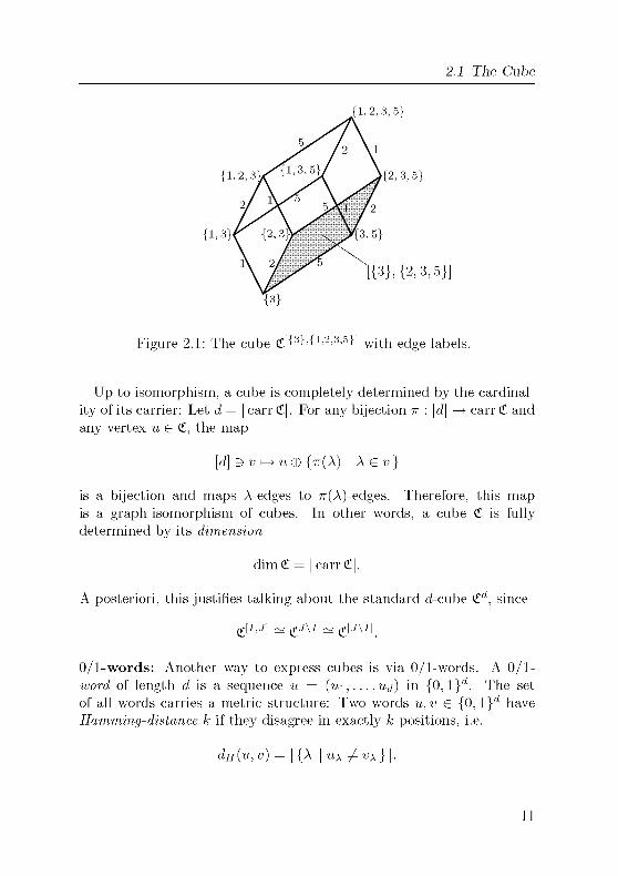
The edges of such a cube are labeled in a natural way: The label of
an edge {u, v} is the unique A G u © v. We will refer to edges with label
A as X-edges. The set of all labels is called the carrier,
carr£[/'J] =J\I.
See Figure 2.1 for an example of a cube.
10
2.1 The Cube
{3}
Figure 2.1: The cube d^^1'2'3'5^ with edge-labels.
Up to isomorphism, a cube is completely determined by the cardinal¬
ity of its carrier: Let d = | carr £|. For any bijection n : [d] —> carr £ and
any vertex u G £, the map
[d] 3 v i-^ w©{tt(A) I A G v}
is a bijection and maps A-edges to 7r(A)-edges. Therefore, this map
is a graph-isomorphism of cubes. In other words, a cube £ is fullydetermined by its dimension
dim£ = | carr £|.
A posteriori, this justifies talking about the standard d-cube £d, since
0/1-words: Another way to express cubes is via 0/1-words. A 0/1-word of length d is a sequence u = (u\,... ,Ud) in {0, l}d. The set
of all words carries a metric structure: Two words u, v G {0, l}d have
Hamming-distance k if they disagree in exactly k positions, i.e.
dH(u,v) = | {A | u\ ^ vx}\.
11

2 Basics
Figure 2.2: The cube £**10*.
From this viewpoint, a d-dimensional cube £d is the graph given by
V(£d) := {0,l}d{u,v}eE(£d) :^=> dH(u,v) = l.
[ '
In fact, as we can identify subsets of [d] with the characteristic vector
(seen as a 0/1-word), this definition of a cube coincides with the previousdefinition. As for sets, we define © as the component-wise operationwith 0©l = l©0=landO©0=l©l = 0.
To express subcubes in the 0/1-world, we extend the alphabet by a
wildcard-symbol *. A word w G {0,1, *}d defines a subcube <tw by
V(£"-) = {WG{0,l}d |VA:WA^* => ux = wx}, (2.3)
i.e., w and u can only differ in labels A for which w\ = *. See Figure 2.2.
The number of *'s in w equals the dimension of £"\ A subcube of
dimension k is called k-face. Furthermore, subcubes of dimension 0, 1
and d — 1 are called vertices, edges and facets, respectively. Similar to
edges we can define the notion of a A-facet. The upper X-facet is the
subcube defined by the word *... *1*...
* consisting of *'s and one 1
at position A. Analogously, the lower X-facet is the subcube defined bythe word *
...*0*
...* consisting of *'s and one 0 at position A.
12

2.2 Unique Sinks
In general, for a subcube defined by w, the antipodal subcube is de¬
fined the following way: Extend © to {0,1, *} by x © * = * © x = * for
x G {0,1, *}. Then, for w G {0,1, *} the antipodal word is w = w©l • • • 1
and <tw is called antipodal to <tw.
1.1 Unique Sinks
Given a graph G = (V, E) a partial orientation is a map </> : L —> V,L Ç E, such that </>(e) G e for all e G L. If L = E we call </> an orientation
of G. For an edge e = {u, v} with </>(e) = v write m —> v. If 0 is clear
from the context we simply write u —> v. The vertex v is called the sink
of e and m is called the source of e. Furthermore, we say e is incoming in
-y, directed towards v, and outgoing from w. The out-degree (m-degree)of a vertex -y is the number of outgoing (incoming) edges incident to v.
Two orientations </> of G = (V, i?) and </>' of G' = (V, E1) are iso¬
morphic if there is a bijection a : V —> y which preserves edges
({w, «} G i? -<=> {a(w),a(w)} G i?') and orientations:
u —> w -<=^> a(w) —> a(w).
In other words, an isomorphism of orientations is a graph-isomorphismwhich maps sinks to sinks.
A vertex o in G is called sink of G if it has no outgoing edges, i.e.,is sink of all incident edges. Accordingly, a source is a vertex with no
incoming edges. In a subcube £' of £, the orientation </> induces an
orientation </>' by0'
^^0
M —> V -<=> M —> W
for an edge {«,«} in £'. The orientations we are interested in have
unique sinks in the induced orientations on all subcubes.
Definition 2.2
A unique sink orientation (USO) of the d-dimensional cube is an orien¬
tation 4> of<td, such that any subcube has a unique sink. More formally,
VI Ç J Ç [d] 3\ue[I,J] VA G J \ I : u © {A} - u. (2.4)
13

2 Basics
Figure 2.3: The leftmost orientation has no global sink. The center ori¬
entation has a global sink but the gray facet has two sinks.
Ergo both orientations are not USOs. The rightmost orien¬
tation is a USO.
For instance, the leftmost orientation in Figure 2.3 has no global sink.
The center one has a global sink but is not a USO since one of its facets
has two sinks. Finally, the rightmost orientation is a USO.
As a small warm-up, we consider low dimensions. The O-dimensional
cube £° consists of exactly one vertex and no edges. Obviously, this
one vertex has no outgoing edges, i.e., is the unique sink. The cube
£1 consists of two vertices u = 0 and v = {1} connected by one edge.There are only two possible orientations, namely <f>i({u,v}) = u and
</>2({«,«}) = v. For </>i the vertex u is the unique sink and for <f>2 the
vertex v is the unique sink. In particular, for vertices and edges the
unique sink property is always satisfied.
The two-dimensional cube £2 has four vertices uq = 0, u\ = {1},«2 = {2}, and us = {1,2}. The edges are {«o,wi}, {""0,1*2}, {wi,w3}and {u2,us,}. An orientation </> assigns to each of these four edges one
of its incident vertices. Thus, there are 16 orientations of £2.
Let 4> be an orientation of £2. If </> has no sink, each vertex has at
least one outgoing edge. Thus, </> must be a cycle. See the left picturein Figure 2.4. Now assume </> has a sink in vq g {uq, ..., «3}. That is,its two incident edges {vq,v\} and {«0,^2} are directed towards vq. In
particular, v\ and V2 have at least two outgoing edges. Thus, for the
out-degree of v\ and V2 three possible cases remain.
14

2 2 Unique Sinks
V2 -^-0«3
wod>-^ 1 v-i
Figure 2 4 The cyclic orientation and the orientation with two sinks
V2
V3/ ^~\Vl
Figure 2 5 The bow and the eye
1 The out-degree of both v\ and V2 is two Then the edges {v\,vs}and {v2,v%} are both directed towards v% Hence, v% is also sink
and 4> is not a unique sink orientation See the picture to the rightm Figure 2 4
2 One vertex has out-degree 1 and the other vertex has out-degree2 Without restriction v\ is the vertex with out-degree 1 Then
the edge {vi,v%} is directed towards v\ In particular, v% is not a
sink Thus, </> is a USO See the picture to the left in Figure 2 5
3 Both vertices have out-degree 1 Then both edges {vi,v%} and
{^2,^3} are outgoing in V3, Again vq is the only sink and </> is a
USO See the picture to the right in Figure 2 5
To construct a 2-dimensional USO we can either use the second case
or the third case of the above enumeration In the second case we first
choose vq G {uq, , «3} and then V2 from the two neighbors of vq The
edges incident to vq we orient towards vq and the edges in V2 we direct
away from V2 This leaves one edge undirected, namely the edge between
the other neighbor v\ of vq and the vertex V3, antipodal to vq By the
first case we have to orient this edge towards v\ to obtain a USO A
15

2 Basics
Figure 2 6 Only bows but no global sink
USO of this type is called a bow Since we have four choices for vq and
then two choices for V2, there are eight bows
In the third case we again choose vq Then we orient the edges incident
to vq towards vq and the edges incident to the antipodal point v% away
from «3 This type of USOs is called an eye Since we only have four
choices for vq, there are four eyes
Definition 2.3
An orientation </> of the d-dimensional cube <td is called 2-USO if every
2-face has a unique sink
In other words, 2-USOs are the orientations which can be composedof eyes and bows It is not too surprising that there are 2-USOs which
are not USOs See e g the orientation in Figure 2 6 However, the
class of 2-USOs is not much larger than the class of USOs As is shown
by Matousek [27], the number of 2-USOs and the number of USOs are
asymptotically of the same order of magnitude in the exponent
2Q(2dlogd) < # ddlm USOg
< # d-dim 2-USOs < 2°(2dlogd)
Furthermore, for acyclic orientations the two classes coincide
16
2 2 Unique Sinks
Theorem 2.4 ([17])An acyclic 2-USO of a cube is a unique sink orientation
For proving Theorem 2 4, we need the following lemma
Lemma 2.5
Let 4> be an acyclic 2-USO Then a sink m </> has a neighbor of out-degree1
Proof Let o be a sink of </> and N(o) the set of all neighbors of o
Assume that every v G N(o) has at least two outgoing edges By this
assumption, for every v G N(o), there is a label A^ with v —> v(B {Xv} ^o Since o, v, v © {A^} and o© {A^} form a 2-face in which o is the sink,we have v © {A^} —> o © {A^}
In particular, </> induces on ./V(o) U {v © {A^} | -y G ./V(o)} a sink-less
orientation Such a graph (and thus </> on the whole cube) contains a
cycle This is a contradiction to </> being cyclic Thus, at least one of
the neighbors of o has out-degree 1 D
Proof of Theorem 2 4 We show by induction on the dimension
that an acyclic 2-USO is a USO
The statement is trivially true for dimension 2 Now assume the
statement is true for dimension d — 1 Let </> be an acyclic orientation
of the d-cuhe, such that every 2-face is a USO By induction all facets
are USOs, since they are (d — l)-dimensional It remains to show that
there is exactly one global sink
In particular, the lower and the upper facets along label d have unique
sinks oi and ou, respectively Since all other vertices have an outgoing
edge in their d-facet, o; and ou are the only candidates for a global sink
If neither o; nor ou is a global sink, then all vertices have at least
one outgoing edge, hence </> contains a cycle By assumption, this case
cannot occur, and at least one of the two vertices has to be a sink
If oi and ou are in a common A-facet, then, by induction, only one is
a sink in this facet, say o = o; Since A^d vertex o is the unique globalsink
The case remains that o; and ou are antipodal and at least one of
them is a global sink We are done if we can rule out the possibilitythat both are global sinks Thus, assume o; and ou are both global
17

2 Basics
Figure 2 7 A cyclic unique sink orientation
sinks A neighbor v of o; is in a common facet with ou In this facet,
ou is a sink So v has an outgoing edge different from v —> o; Thus, no
neighbor of o; has out-degree 1 in contradiction to Lemma 2 5 D
The following question arises Are there cyclic USOs7 Figure 2 7
answers this question affirmatively
2.3 Complexity Issues
Given a USO, the goal is to find its sink As there are 2°(2dl°sd) USOs
of dimension d (see [27]), at least Q(2d\ogd) bits are needed to encode
a particular USO Thus, if the USO is given explicitly as input to an
algorithm, we can find the sink in time linear in the input size by just
scanning through the vertices
We will, however, adopt a different complexity model A USO is given
implicitly by an oracle Such oracle, when queried in a vertex, reveals
the orientation in this vertex
Definition 2.6
Given a unique sink orientation </> on a cube £, the outmap s of'</> is the
map assigning to every vertex the labels of outgoing edges, l e,
s V(£)^2carr£ , v^{X \v^v®{X}}
18

2.3 Complexity Issues
Any algorithm can access the outmap of a USO only via an oracle.
That is, the algorithm can ask for the outmap in one vertex at a time.
The task is to query the sink. The running time is measured in the
number of queries to the oracle.
As we will learn in the next chapter, many problems (such as linear
programming) can be transformed into unique sink orientations in such a
way that finding the sink of this orientation solves the original problem.More concretely, given some problem V, we want to define an oracle for
a USO based on V. This oracle should be able to perform a vertex query
fast. Furthermore, after querying the sink of the USO, the solution to
V can be found fast. Hence, an oracle consists of two algorithms. One
algorithm computes s(v) from V. The other algorithm determines the
solution of V given the sink of s. If both algorithms have a polynomial
running time, the oracle is called polynomial-time unique sink oracle.
For such oracles, an algorithm finding the sink in a USO solves the
original problem with an additional polynomial factor.
Obviously, 0(2d) queries are enough to find the sink of a USO, since
after querying all 2d_1 vertices of even cardinality, we know the entire
orientation. We aim for algorithms asking only o(2d) queries. In conse¬
quence, we know only o(d2d) edges of the orientation. Such an algorithmis unable to verify whether the oracle was based on a USO.
Let </> be a partial orientation on a cube, such that exactly two adja¬cent edges ei = {v © {Ai},«} and &2 = {v,v ® {A2}} are not oriented.
In the 2-face £0 spanned by the vertex v and the labels Ai and A2, onlythe orientation in the vertex v = v © {Ai, A2} antipodal to v is known.
Let </>' be an extension of </> such that
v - v © {AJ «=> v - v © {AJ
for 1 = 1, 2. A closer look at Figure 2.5 shows that then £0 can neither be
an eye nor a bow, so </>' is not a USO. In consequence, it is undecidable if
an orientation is a USO as long as the orientation of less than (d— \)2d~1edges is known, since then there is at least one vertex for which the
orientation of two incident edges are unknown.
Definition 2.7
Given an outmap s on a d-dimensional cube, we consider the following
algorithmic problems:
19
2 Basics
• Sink is the problem of querying the sink of s provided that s is a
unique sink orientation
• SinkOrFalsify is the problem of either querying a sink of s or
Ending a certificate for s not being a unique sink orientation
If we know a bound on the number of queries for some algorithm
solving Sink, then this algorithm also solves SinkOrFalsify If the
algorithm needs too many queries on some orientation, the sequence of
queried vertices is a certificate that this orientation is not a USO
Definition 2.8
For a deterministic algorithm A and a unique sink orientation s, let
ïa(s) be the number of queries ofA until the sink is queried The worst
case behavior of A is defined by
^A(d) =max{t^(s) | s d-dim USO}
Furthermore, let t(d) be the minimal t^{d) over all deterministic al¬
gorithms A solving Sink
For randomized algorithms, m analogy to the deterministic case we
define t
Definition 2.9
For a randomized algorithm A and a unique sink orientation s, let tyi(s)be the expected number of queries of A until the sink is queried The
worst case behavior of A is defined by
tA{d) =max{ty4(s) | s d-dim USO}
Furthermore, let i(d) be the minimal t^(d) over all randomized algo¬rithms A solving Sink
In both definitions the algorithm has to query the sink in order to
terminate For example, in dimension 0 any algorithm needs exactlyone query to find the sink, although we know the position of the sink
20

2.4 Remarks
2.4 Remarks
The notation presented in this chapter follows [42]. To the best of our
knowledge, USOs in their full generality were first studied in [42] as inde¬
pendent objects, even though the connection with linear programming
or linear complementarity problems has been made by other authors
before [40, 1]. The smaller class of acyclic USOs appeared much earlier
under several different names, e.g. pseudo-Boolean functions [16], ab¬
stract objective functions [1], and completely unimodular numberings
[18].Having Theorem 2.4 in mind, one might hope that the acyclic USOs
can further be distinguished from general USOs. In fact, for acyclicUSOs there exists a randomized algorithm which requires a subexpo-nential number of queries [9, 10]. For general USOs, no such algorithmis known. In contrast, the question about the number of acyclic USOs
is still open.
Let us point out that the complexity model introduced in this chapterhas to be handled with care. Not only is it necessary that the transition
between concrete problems and USOs is polynomial. In addition, we are
only counting the number of vertex evaluations an algorithm requires.
Thus, in theory, between two vertex evaluations, an algorithm for findingthe sink in a USO can spend exponential time without increasing its
"running time". However, so far, no algorithm for this problem actuallymakes use of this additional power. The main reason is that we do not
know how to use it.
21

2 Basics
22

3 Sources
There was a red-haired
man who had no eyes or
ears Neither did he have
any hair, so he was called
red-haired theoretically
(Daniil Kharms)
23

3 Sources
In this chapter we will often consider Rd as a vector space. From
now on we fix the standard basis {ei,..., e<J of unit vectors. In par¬
ticular, linear functions and matrices are identified with respect to the
standard basis. Furthermore, we use the standard scalar product (,}on Rd. The symbol I denotes the identity matrix of the appropriatedimension. Also 0 represents the origin of the appropriate space. If
not defined otherwise, operations are performed component-wise. For
instance, R := {x G Rn | x > 0 } is the set of all non-negative vectors
in Rn, also known as the non-negative orthant.
3.1 Linear Programming
In linear programming, the aim is to maximize a linear function over a
polyhedron. A polyhedron is defined as the intersection of finitely many
half-spaces. A bounded polyhedron is called polytope. In the following,we will restrict our attention to polyhedra of the form V = TL n R,where TL is an affine subspace of Rn. In this setup, a polyhedron is fullydetermined by a matrix A G Rmxn and a vector b G Rm, namely
TL{A,b) := {xeMn\Ax = b} (3.1)
V(A,b) := H(A,b)nMrl = {xeMn \Ax = b, x>0}.(3.2)
In fact, up to affine transformation every polyhedron can be described
by a V(A, b). For more details on polytopes and polyhedra see [44].For a simple example, see Figure 3.1.
A linear program is defined by a matrix A G Rmxn and vectors b G Rm
and c G Rn. The goal is then to solve the following problem:
max cTx
such that Ax = b
x > 0,
that is, we want to maximize the linear function x i—> cTx over the
polyhedron V(A, b). We denote this linear program by LP(A, 6, c). The
function x i—> cTx is called objective function.A polyhedron may be empty or may contain points with arbitrary
large values of cTx. In these cases, the linear program is called infeasible,
respectively unbounded.
24
3 1 Linear Programming
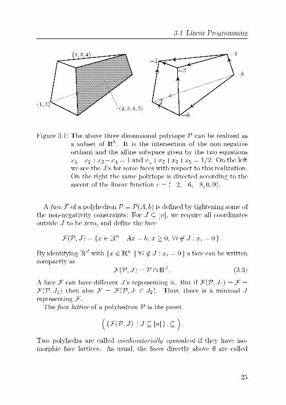
Figure 3.1: The above three-dimensional polytope V can be realized as
a subset of R5. It is the intersection of the non-negativeorthant and the affine subspace given by the two equations
x\-\-X2 +a?3 — X4 = 1 and X1+X2+X3 + X5 = 1/2. On the left
we see the J's for some faces with respect to this realization.
On the right the same polytope is directed according to the
ascent of the linear function c = (—2, —6, —8, 0, 0).
A face J7 of a polyhedron V = V(A, b) is defined by tightening some of
the non-negativity constraints: For J Ç [n], we require all coordinates
outside J to be zero, and define the face
T(V, J) = {x G Rn I Ax = b, x > 0, V« £ J : xt = 0 } .
By identifying RJ with {x G Rn | V« ^ J : xt = 0 } a face can be written
compactly as
T(V, J) = PnRJ. (3.3)
A face T can have different J's representing it. But if T(V, J\) = T =
T(V,J2) then also T = T{V,J\ n J2). Thus, there is a minimal J
representing T.
The face lattice of a polyhedron V is the poset
{{HV,J) I JÇ[n]},ç).Two polyhedra are called combinatorially equivalent if they have iso¬
morphic face lattices. As usual, the faces directly above 0 are called
25

3 Sources
vertices, the faces directly above vertices are edges and facets are the
faces directly below V
If a linear program has a finite optimal value, the optimum is alwaysattained in a vertex Thus, from a combinatorial point of view, we can
abstract from the concrete values and consider only the ordering of the
vertices induced by the objective function To avoid technical problemswe restrict ourselves in this section to polytopes For polytopes any
objective function yields a finite optimum
Definition 3.1
An abstract objective function on a (combinatorial) polytope V is a
partial order < of the vertices of V, such that every face has a unique
maximal vertex
Abstract objective functions were first defined by Alder and Saigal
[1] They provide the general framework in which the first combinatorial
subexponential algorithm RandomFacet [21] works
In a sufficiently generic linear program, the linear function c assigns
a different value to each vertex (If two vertices have the same value,a slight perturbation of c resolves this problem ) Order the vertices
according to their values, l e,set u -< v if cTu < cTv Then the relation
-< is a finite linear order on the set of vertices In particular, every set
of vertices has a maximum and -< defines an abstract objective function
on V Thus, abstract objective functions are a generalization of linear
programming
Moreover, abstract objective functions are the link between linear pro¬
gramming and unique sink orientations Any abstract objective function
defines an orientation of the edge-graph of V for an edge {u, v}, direct
u —> v -<=> u -< v (3 4)
With this orientation, a maximum of a face is a sink of this face Con¬
sequently, if we start with an abstract objective function, every face has
a unique sink
Definition 3.2
A unique sink orientation of a polytope V is an orientation of the edge
graph of V, such that every face has a unique sink
26
3 1 Linear Programming
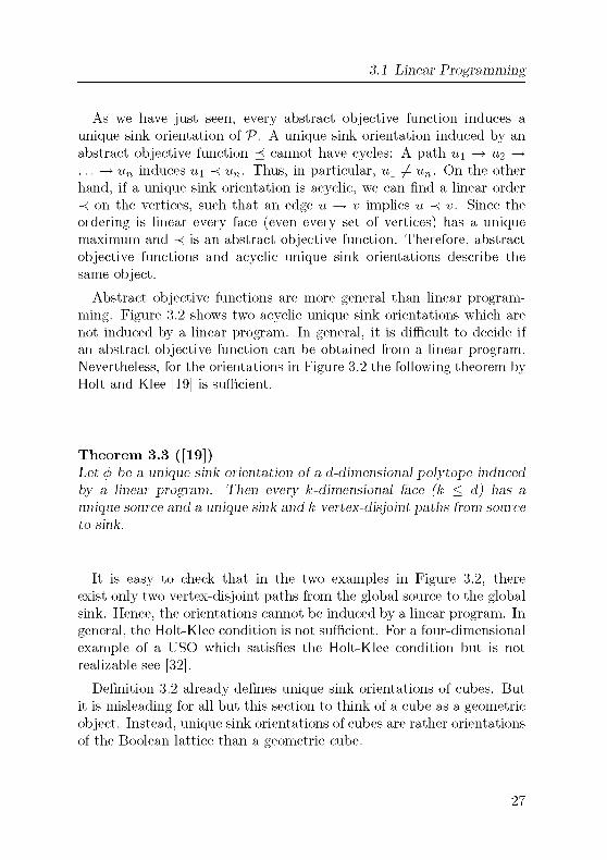
As we have just seen, every abstract objective function induces a
unique sink orientation of V A unique sink orientation induced by an
abstract objective function < cannot have cycles A path u\ —> «2 —>
—> un induces u\ -< un Thus, in particular, u\ ^ un On the other
hand, if a unique sink orientation is acyclic, we can find a linear order
-< on the vertices, such that an edge u —> v implies u -< v Since the
ordering is linear every face (even every set of vertices) has a unique
maximum and -< is an abstract objective function Therefore, abstract
objective functions and acyclic unique sink orientations describe the
same object
Abstract objective functions are more general than linear program¬
ming Figure 3 2 shows two acyclic unique sink orientations which are
not induced by a linear program In general, it is difficult to decide if
an abstract objective function can be obtained from a linear program
Nevertheless, for the orientations in Figure 3 2 the following theorem byHolt and Klee [19] is sufficient
Theorem 3.3 ([19])Let 4> be a unique sink orientation of a d-dimensional polytope induced
by a linear program Then every k-dimensional face (k < d) has a
unique source and a unique sink and k vertex-disjoint paths from source
to sink
It is easy to check that in the two examples in Figure 3 2, there
exist only two vertex-disjoint paths from the global source to the globalsink Hence, the orientations cannot be induced by a linear program In
general, the Holt-Klee condition is not sufficient For a four-dimensional
example of a USO which satisfies the Holt-Klee condition but is not
realizable see [32]
Definition 3 2 already defines unique sink orientations of cubes But
it is misleading for all but this section to think of a cube as a geometric
object Instead, unique sink orientations of cubes are rather orientations
of the Boolean lattice than a geometric cube
27

3 Sources
Figure 3.2: Two acyclic USOs which are not induced by a linear pro¬
gram. The two highlighted paths share the vertex v.
3.2 Linear Complementarity Problems
Given a matrix M G Rnxn and a vector q G Rn, the linear complemen¬
tarity problem LCP(M, q) is to find vectors w, z G Rn, such that
= q
> 0
> o
= 0
is satisfied. Obviously, such vectors do not exist for all M and q. For
instance, w — Mz = q might not be solvable. But if the vectors exist,then for i with wt > 0 the coordinate zt has to be 0 and vice versa
(since w,z are non-negative). In other words, the non-zero entries of a
solution to LCP(M, q) are complementary.
In the following discussion we will restrict our attention to so-called
P-matrices, i.e., matrices for which all principal minors are positive. P-
matrices are such that their corresponding LCP is always solvable, for
any q.
w - Mz
w
z
Tw z
28

3.2 Linear Complementarity Problems
Theorem 3.4 ([37])A matrix M G Rnxn is a P-matrix if and only if for ail q G R the
linear complementarity problem, LCP(M, q), has a unique solution.
For a proof, see e.g. [6, Chapter 3.3].If we knew the orthogonal coordinate subspaces R-" and RM^ in
which the solution w*, z* of LCP(M, q) lives in, i.e., if we knew v* Ç [n],such that w* G R^* and z* G R^-"*, the vectors w* and z* would solve
w — Mz = q
w G R^* (3.5)z e jrMV;*.
For a P-matrix (3.5) is a system of linear equations in 2n variables of
rank 2n. Hence, knowing v* solves the LCP (up to solving this system
of linear equations).The equation system (3.5) can be simplified in the following way:
For v Ç [n] and matrices A = (a»j)j,je[n] and B = {blJ)l^^[n-\ define
(A | B)v to be the matrix with the columns of A at position j G v and
the columns of B otherwise, i.e.
«A | *)„)., = { £ HVV. (3.6)
For i£l' and y G R^-", we get
(A | B)v(x + y)=Ax + By.
Let I represent the identity matrix (of the appropriate dimension).Hence, for w G R-" and z G R^-", we want to solve:
q = w - Mz = (I | -M)v(w + z).
The determinant of (I | —M)v equals (up to its sign) the determinant
of the [n] \ «-minor of M. Thus, for a P-matrix, the system of linear
equations has a unique solution, namely
x(v) = (I | -M)v-lq.
As w and z are complementary one can extract w and z from x by
setting Wj = x(v)j, z3 = 0 for j G v and z3 = x(v)j, w3 = 0 otherwise.
29

3 Sources
(i i iv-
Fmd w, z G R3 with
1 2 0'
\ ( 1
0 1 2 )z= 1
2 0 1 1 \1w > 0
z > 0
w1 z = 0
X-i i -i)
1 -1 3)
.
1_
1_
1
Figure 3 3 An LCP and its orientation The vertices are labeled bytheir x(v) The highlighted edges form a cycle
Since x(v) is unique for all -y's, a strategy for solving LCP(M, q) would
be to guess v and calculate x(v) If x(v) is a non-negative vector this
solves the LCP If not, proceed with a different v
Definition 3.5
For a P-matrix MeB1 and q G Rn, dehne an orientation on £ by
©{A} ((I | -M)-lq)x < 0 (3 7)
As we just discussed, a sink of this orientation would yield the solu¬
tion of LCP(M, q) Also, the matrix (I | —M)v ,and therefore the
orientation in a vertex, can be computed in polynomial time In other
words, if the orientation is a USO this introduces a polynomial-time
unique sink oracle for linear complementarity problems See Figure 3 3
for an example of a cyclic USO defined by an LCP
Theorem 3.6 ([40])For a P-matrix M G Rnxn and q G Rn the orientation m Definition 3 5
is a unique sink orientation of £
The crucial observation for the proof of Theorem 3 6 is that a subcube
[/, J] of £ corresponds to the problem of finding w G RJ and z G rI^1
30
3.3 Strong LP-type Problems
with w — Mz = q, wTz = 0 and wt,zt > 0 for i G J \ I, which again is
a linear complementarity problem. For details see [40].
3.3 Strong LP-type Problems
Let us look once more at the reduction from LCP's to USOs, now from
quite far away. The reduction associates to each subcube [/, J] of £ a
problem by strengthening/weakening constraints not in J \ I. Namely,for i ^ J we require wt = 0 but relax zt > 0 and for i G / we require
zt = 0 and relax wt > 0. The key observation is that for I = J, i.e., for a
vertex of £, the corresponding problem is a system of linear equationsand can be solved easily.The goal of this section is to work out a framework under which sim¬
ilar reductions for optimization problems over the non-negative orthant
yield a USO. Motivated by the LCP-reduction, a possible attempt to
transform such a problem to a USO is the following: To sets I Ç. J Ç. [d](i.e., faces [/, J]) associate a domain (by strengthening/weakening the
positivity constraints not in J \I) and solve the optimization problemover this domain. Then compare the solutions. We do this in the hopethat the case I = J again is easy. This way we assign to a face given
by I Ç J C [d] a value w(I, J). On an abstract level we order the set of
faces.
Definition 3.7
Let (O, <) be a poset and w a mapping from the pairs (I, J) of sets
I Ç J C [d] to O. Then w is called monotone if for all I Ç J C [d] and
I'QJ'Q [à]
ICI'and J Ç J' => w(I,J)<w(I',J'). (3.8)
It is called local if for all I\ Ç J\ C [d] and I2 Ç J2 C [d]
w{h, Ji) = w(I2, J2) ,00^
«=^ w(h n l2, Ji n J2) = w(h u l2, Ji u J2).^ ' '
If w is monotone and local, the tuple (d, w, O, <) is called a strong LP-
type problem. Tiie value of a strong LP-type problem (d,w,0,<) is
w(<D,[d\).
31

3 Sources
Monotonicity for w does not refer to the face structure of £d. For
I Ç J C [d] and I' Ç J' C [d] the face [/, J] is a subface of [/', J'] if and
only if I' C I C J C J'. In contrast, w is monotone with regard to the
component-wise inclusion relation on pairs of sets
(I, J) Ç (I', J') «=^ I Ç J"' and J Ç J'. (3.10)
For monotone w's the -<=-direction of locality is already satisfied. For
II - Ji - [d] and I2 Ç J2 C [d], obviously (for A; = 1, 2)
(h n j2, Ji n J2) ç (4, Jfc) ç (h u j2, Ji u J2)
and therefore, by monotonicity,
w(l1nl2,J1nJ2) <w(lk,Jk) < w(l1ul2,J1uJ2)
= w{l1nl2,JinJ2).
In particular, all four values are equal. Thus, for strong LP-type prob¬lems we can (and will) use the following form of locality:
w(I1,J1) = w(I2,J2) =>
w(l1nl2,J1r\J2)=w(luJ1) (3.11)= w(J2lJ2)=M(I1UJ1,J2UJ2).
In general, the optimization problem corresponding to the value of a
strong LP-type problem will be difficult to solve. But for a vertex v the
value w(v, v) can be found easily. A generic case for an LP-type problemis to optimize some function / over the non-negative orthant. Subcubes
[/, J] correspond to a strengthening of the positivity constraints on co¬
ordinates not in J and a weakening on coordinates in I. In other words,we drop all conditions on i„ 1 G / and require x3 = 0 for j ^ J. For
1 = 9 and J = [d], we get the original problem over the non-negativeorthant.
For I = v = J the problem simplifies to optimizing / over R^. Thus,after restriciting / to ffV, we have to solve an unconstrainted opti¬mization problem. For a well-behaving function /, this can be solved
efficiently. Hence, the aim of an abstract strong LP-type problem is to
find a vertex v with w(v,v) = w(0, [d]).
32

3 3 Strong LP-type Problems
Definition 3.8
Let (d,w,0,<) be a strong LP-type problem and I Ç J C [d] A
vertex v, I Ç v Ç J, is called a basis of [I, J] with respect to w if
w{v, v) = w(I, J)
We want to find a basis of [/, J] to determine w(I, J) In consequence,
even if we would find a basis we could not verify it by its definition A
local condition is needed and can be provided by locality of w Since
w(v, v) = w(I, J) for a basis v, (3 11) yields
w(I, v) = w(I Pi v, J Pi v) = w(I U v, J U v) = w{v, J)
Furthermore, by monotonicity the w-value of an edge [v, v U {A}] with
A G J \ v is sandwiched between w(v, v) and w(v, J) = w(v, v) and the
w-value of [v \ {/j,},v\, ^ G v \ I is sandwiched between w(I,v) and
w(v, v) = w(v, J) Therefore, all these values are equal and v is a basis
of all its incident edges m [/, J]
Lemma 3.9
For a strong LP-type problem (d,w,0, <), a vertex v is a basis of a
subcube [I, J] if and only if it is a basis of all edges [v \ {A}, v U {A}],AG J\I
Proof As we just argued for a basis v of [/, J], the incident edges
(l e,all {v © {A}, v}, X G J \ I) have basis v
Now assume v is a basis of its incident edges m [/, J] We will distin¬
guish between edges towards subsets and edges towards supersets of v
and show that w(I,v) = w(v,v) = w(v,J) But then, by monotonicity,
w{v, v) = w(I, v) < w(I, J) < w{v, J) = w{v, v)
and v is a basis of [/, J]For the equation w(v,v) = w(I,v) we have to show that v is a basis
of [v \ {A}, v] for A G v \ I Let v \ I = {Ai, A,J By induction on k
and locality, the equations w(v,v) = w(v \ {AJ,-y) imply
w(v,v) = w(v\ {Ai, ,AJ,-y),
hence w(v, v) = w(v \(v\ I), v) = w(I, v) The same arguments for the
edges [v, v U {A}], A G J \ v proves w(v, v) = w(v, J) D
33
3 Sources
So far, we cannot guarantee the existence of a basis But, what if
there is a basis v of [I, J]7 If we divide [/, J] along a label A G J \ I
then the A-facet of [/, J] containing v must have the same w-value as
[/, J] This is a direct consequence of Lemma 3 9 Therefore, a basis
has a chance to exist mamly m strong LP-type problems of the following
type
Definition 3.10
A strong LP-type problem (d, w,0,<) is called reducible if for any two
sets I Ç J C [d] and A G J \ I, the value w(I, J) is attained m the
X-facets of [I, J], l e
w(I, J) G {w(I U {A}, J), w(I, J \ {A})}
If w is reducible then recursively we can trace the w-value of a cube
[/, J] over facets, ridges and so forth down to vertices Thus, reducible
strong LP-type problems have bases Furthermore, for two bases v\ and
V2 of [/, J], by definition, w(v\, v\) = w(I, J) = w(v2, v2) Therefore, by
locality m the form of (3 11) we can conclude that w(v\ n v2, «ifl^) =
w(vi, v{) = w(I, J) and v\ n V2 is a basis Hence, the inclusion-minimal
basis is unique This proves the following lemma
Lemma 3.11
Let (d, w, O, <) be a reducible strong LP-type problem and I Ç J C [d]Then there is a unique inclusion-minimal basis of [I, J]
For a reducible strong LP-type problem (d,w,0, <) the value of an
edge [v, v U {A}] is either equal to w(v,v) or to w(v U {X},v U {A})Furthermore, by monotonicity
w(v, v) < w(v, v U {A}) < w(v U {A}, v U {A})
It is possible that both v and v U {A} are a basis But v is the inclusion-
minimal basis of [v,v U {A}] if and only if it is a basis If v is not
basis, then w(v, v) < w(v, v U {A}) and v U {A} is the inclusion-minimal
basis Thus, if we orient the cube such that an edge points towards its
inclusion-minimal basis then »-»»U {A} hods if and only if w(v, v) <
w(v, v U {A}) This yields a unique sink orientation
34
3 3 Strong LP-type Problems
Theorem 3.12
Let (d, w,0,<) be a reducible strong LP-type problem Then the ori¬
entation of <td defined by
»-»»U {A} -<=> w{v, v) < w{v, v U {A})
is a unique sink orientation Furthermore, the sink of a subcube [I, J]is a basis of [I, J]
Proof We orient the cube m such a way that edges point towards
their inclusion-minimal basis Given a subcube [/, J] of £d and a sink
o G [/, J], then o is inclusion-minimal basis of all its incident edges m
[/, J] In particular, by Lemma 3 9, o is a basis of [/, J] It is also
inclusion-minimal as basis of [/, J] If o was not inclusion-minimal we
would find a basis o' Ç o with w(o', o') = w(o, o) By locality we can
assume that o' and o differ m only one element Hence, o would not be
an inclusion-minimal basis of the edge {o', o}On the other hand, by Lemma 3 9, an inclusion-minimal basis v of
[/, J] is a basis of all its incident edges If v is not inclusion-minimal on
one edge, say {-y©{A}, v}, then A has to be m v and w(-y©{A}, -y©{A}) =
w(v, v) But then v © {A} is also a basis of [/, J] and v not inclusion-
minimal
In conclusion each sink m [/, J] is a inclusion-minimal basis of [/, J]By Lemma 3 11 [/, J] has exactly one such basis, l e
, [/, J] has a unique
sink D
In order to find the orientation m a vertex we need to compute if
w(v, v) < w(v,v © {A}) for all A G [n] This can also be done by
evaluating w(v © {X},v © {A}) Thus, a vertex evaluation m the USO
of Theorem 3 12 corresponds to at most d + 1 evaluations of the form
w{v, v)For the remainder of this section, we study the reverse question For
which USO s can we find a reducible strong LP-type problem inducings7 Let s be a USO on £d induced by some reducible strong LP-type
problem (d, w,0,<) The w-value of a subcube [/, J] of £d is given bythe w-value of the sink of [/, J] Denote with <r(/, J) the sink of such a
subcube [/, J] Then s is induced by w if and only if
w{I,J) = w{o-{I,J),o-{I,J)) (3 12)
35
3 Sources
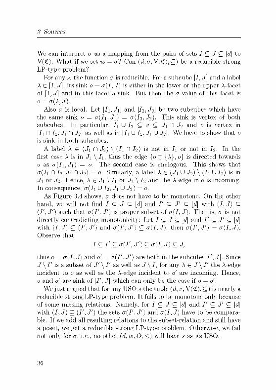
We can interpret a as a mapping from the pairs of sets I C J G [d] to
V(£). What if we set w = a? Can (d, a, V(£), Ç) be a reducible strong
LP-type problem?For any s, the function a is reducible. For a subcube [I, J] and a label
A G [I, J], its sink o = a (I, J) is either in the lower or the upper A-facet
of [I, J] and in this facet a sink. But then the a-value of this facet is
o = a(I,J).Also a is local. Let \I\, J\] and [I2, J2] be two subcubes which have
the same sink o = a(I\,Ji) = a(I2,J2). This sink is vertex of both
subcubes. In particular, I\ U I2 G v G J1 n J2 and o is vertex in
[Il n I2, J\ n J2] as well as in \I\ U I2, J\ U J2\. We have to show that o
is sink in both subcubes.
A label A G (J\ n J2) \ (I\ n I2) is not in I\ or not in I2. In the
first case A is in J\ \ I\, thus the edge {o © {A}, 0} is directed towards
o as <t(/i, Ji) = o. The second case is analogous. This shows that
<t(/i n I2, J\ n J2) = o. Similarly, a label A G (J\ U J2) \ (I\ U J2) is m
J\ or J2. Hence, A G J\ \ I\ or J2 \ I2 and the A-edge in o is incoming.In consequence, cr(Ii U I2, J\ U J2) = 0.
As Figure 3.4 shows, <r does not have to be monotone. On the other
hand, we will not find J Ç J Ç [d] and I' G J' G [d] with (I, J) G
(/', J') such that a(I', J') is proper subset of a (I, J). That is, a is not
directly contradicting monotonicity: Let I G J G [d] and I' G J' G [d]with (I, J) G (/', J') and a{I',J') G a{I,J), then a{I',J') = a(I,J).Observe that
I CI' Ç a(I', J') G a (I, J) Ç J,
thus o = a (I, J) and o' = a(I', J') are both in the subcube [/', J]. Since
J \ I' is a subset of J' \ I' as well as J\I, for any A G J\I' the A-edgeincident to o as well as the A-edge incident to o' are incoming. Hence,o and o' are sink of [/', J] which can only be the case if o = o'.
We just argued that for any USO s the tuple (d, a, V(£), Ç) is nearly a
reducible strong LP-type problem. It fails to be monotone only because
of some missing relations. Namely, for I Ç J G [d] and I' Ç J' G [d]with (/, J) Ç (/', J') the sets a(I', J') and a (I, J) have to be compara¬
ble. If we add all resulting relations to the subset-relation and still have
a poset, we get a reducible strong LP-type problem. Otherwise, we fail
not only for a, i.e., no other (d,w, O, <) will have s as its USO.
36

3 3 Strong LP-type Problems
Figure 3 4 The map a might be not monotone The highlighted sub-
cube [0, {2, 3}] has sink {2} whereas the whole cube has sink
{1}
Proposition 3.13
A unique sink orientation on £ with outmap s is induced by a reducible
strong LP-type problem if and only if the digraph on V(£)
u ~» v «=> ii\»C[(i]\ (s(u) U s(v)) (3 13)
is acyclic except for loops
Proof Let < be the transitive closure of ~->, i e
u ^ v -<=> 3«i, , Wfc u -^ u\ -^ -^ U]. -^ v
Since for u G v the set u\v is empty, ~-> and therefore < is a refinement
of Ç In particular, < is reflexive It is transitive by definition Finally,it is antisymmetric if and only if (V(£), ~->) has no other cycles except
loopsIf the relation < is antisymmetric, (d, a, V(£), <) can be shown to be
a reducible strong LP-type problem As we argued above, a is alreadyreducible and local For monotonicity, let (I, J) Ç (/', J'), J' C [d] and
o = a (I, J), o' = a(I', J') We have to show that o < o' Since o is
the sink in [/, J] for A G J \ I the A-edge incident to o is incoming,
37

3 Sources
i.e., A e- s(o). Hence, J\ I G [d}\ s(o). Similarly, J' \ V G [d] \ s(o').Furthermore, since o G J C J' and / Ç V G o', a A G o \ o' is in J but
not in V, we conclude
o \ o' G J \ I' G J \ I n J' \ I' G [d] \ s(o) n [d] \ s(o').
Thus, o ~-> o'.
We just showed that (d, a, V(£), <) is a reducible strong LP-type prob¬lem if and only if < is a poset which is the case if and only if ~-> is
acyclic besides loops. Furthermore, for an edge {v,v U {A}} the value
a(v, v U {A}) y^ v = a(v, v) if and only if v —> v U {A}. Hence, s is the
orientation defined by (d, a, V(£), <).On the other hand, let (d, w, O, <) be a reducible strong LP-type
problem which induces s as its USO. For the relation < defined by s let
us first prove
u < v =4> w{u, u) < w{v, v).
As < is the transitive closure of ~->, it is enough to show the statement
for pairs u ~-> v. For such a pair by definition u\v is a subset of [d] \ s(u)and [<i] \ s(v). In particular, m \ (u n w) = m \ w is disjoint from s(u) and
(m U v) \ v = u \ v is disjoint from s(v). Hence, m is a sink in \u n v, u]and v is a sink in [v,u U v]. As s is the USO corresponding to w, byTheorem 3.12 and monotonicity of w we get
w{u, u) = w{u C\v,u) < w{v, uL) v) = w{v, v).
We will show that < is antisymmetric. Take three vertices u,v,v'with u ~-> v < v' < u. As we just showed, for such u, v and v' the
inequality
w{u,u) < w{v,v) < w(v',v') < w{u,u)
must hold. Therefore, w(u, u) = w(v, v) and by locality the two values
w(uC\v,uC\v) and w(uL)v, uUv) are equal. Assume there is a A G u\v.Since u ~-+ v, this label A is not in s(u). Thus, the edge {u \ {A},m} is
directed towards u. As the orientation s is defined by w the vertex u
is a sink of {u \ {A}, u} if and only if w(u \ {A}, u \ {A}) < w(u \ {A}).Hence
w{uC\v,uC\v) < w{u \ {A}, u \ {A})
38
3.3 Strong LP-type Problems
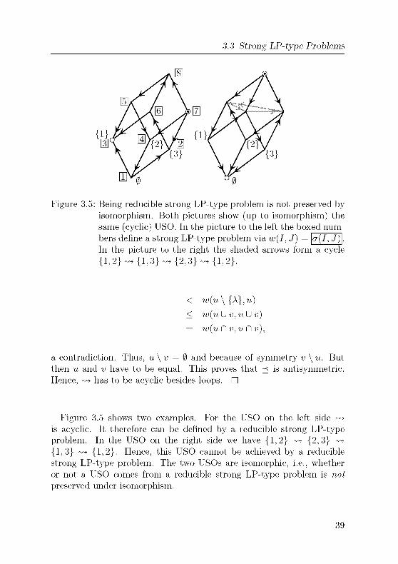
Figure 3.5: Being reducible strong LP-type problem is not preserved by
isomorphism. Both pictures show (up to isomorphism) the
same (cyclic) USO. In the picture to the left the boxed num¬
bers define a strong LP-type problem via w(I, J) = a (I, J)In the picture to the right the shaded arrows form a cycle
{1,2} -{1,3} -{2, 3} -{1,2}.
< w(u \ {A}, u)
< w(u L) v,uL) v)
= w(u nji,«n v),
a contradiction. Thus, u \ v = 0 and because of symmetry v\u. But
then u and v have to be equal. This proves that < is antisymmetric.
Hence, ~-> has to be acyclic besides loops. D
Figure 3.5 shows two examples. For the USO on the left side ~->
is acyclic. It therefore can be defined by a reducible strong LP-type
problem. In the USO on the right side we have {1,2} ~-> {2,3} ~->
{1,3} ~-> {1,2}. Hence, this USO cannot be achieved by a reducible
strong LP-type problem. The two USOs are isomorphic, i.e., whether
or not a USO comes from a reducible strong LP-type problem is not
preserved under isomorphism.
39

3 Sources
3.4 Strictly Convex (Quadratic) Programming
A function / : D —> R over a convex set D G Rd is strictly convex if for
any x,y G D and 9 G [0,1] the inequality
f(ex + (i-e)y)<ef(x) + (i-e)f(y)
holds with equality only for 6 = 0,1. Laxly speaking, the line segment
connecting two points on the curve {(x, f(x)) | x G D } is always above
the curve. If a strictly convex function / attains its infimum over D, it
does so in a unique minimizer x*(D). If there would be two minimizers
x\ and X2 in D the line between these two would be above the curve of
/ and therefore either /(#i) or f(x2) is not minimal.
In the following we will restrict to continuously differentiable strictlyconvex functions /. For such / the gradient
v/=ß^,...,^\dxi
' '
dxd
not only exists but determines minimizers:
Lemma 3.14 ([35, Chapter 2, Exercise 10])Let D G Rd be a convex set and /:fl-*Ba continuously differentiable
strictly convex function. Then a point x* minimizes f over D iff
Vx G D : V/(x*)(x-x*) >0. (3.14)
For an inner point x* the condition (3.14) is equivalent to the equation
V/(x*) = 0. Thus, the statement is mainly interesting for boundary
points. In particular, if D is not full-dimensional, every point in D is a
boundary point.
Proof. For a unit vector u G Rd, ||w|| = 1, the (one-sided) direc¬
tional derivative of / along m at a point x G D is
v-7 r, n rf(x + eu) - f{x)
V„/(x)= hm
.
e^o+ e
We consider only the limit from above, as the points we are interested
in very well can be on the boundary of D. In particular, V„/(x) is not
40

3 4 Strictly Convex (Quadratic) Programming
defined for all u The limit only exists if x + eu G D for sufficiently small
e
By the chain rule applied to / and g t >—> x + tu, the directional
derivative and the gradient are connected by
V„/(x)=V/(x) u
We use directional derivatives to show that x* is a mimmizer of /
By scaling with ||x — x*||, (3 14) can be equivalently formulated as
V«/(x*) > 0 for all unit vectors u for which it is defined Here we need
convexity of D By convexity, V«/(x*) is defined if there exists some x
with x — x* = ||x — x*||wFirst assume there is a unit vector u with V«/(x*) < 0 Then for
sufficiently small e, the vector x* + eu is in D and
fjx*+eu)-fjx*)^Q
e
In particular, x* + eu proves that x* is not minimal
Now assume that x* does not minimize / Then there is a point x G D
and some A > 0 with /(x) = f(x*) — A Since / and D are convex for
any 9 G [0,1] the point (1 — ff)x* + ox is in D and has /-value
/((l - 6)x* + ex) < (1 - 6)f(x*) + 6f(x) = f{x*) - 6A
Hence, for all e, 0 < e < ||x — x*|| and u = (x — x*)/||x — x*|| we get
f{x* + eu)-f{x*)<
A< o^
e~
\\x — x*\\
which shows V„/(x*) < 0 D
The problem of strictly convex programming is to minimize a strictlyconvex function / over the non-negative orthant, l e
,we want to find
x* with
fix*) =min{/(x) | x >0} (3 15)
which if exists, is unique The mam problem for such programs is caused
by the non-negativity constraints The unconstrained variant to mini¬
mize / (even over some linear subspace RJ) is considerably easier and
(for suitable /) can be solved using analytical methods
41

3 Sources
Again we have the situation that the problem we are interested in
is difficult, but modifying the constraints we end up with a solvable
problem. This suggests to connect to strong LP-type problems. For
I Ç J C [d] consider the set
C{I, J) := {x G Rd | xt > 0 for i g I, xt = 0 for i G* J) . (3.16)
In other words, starting from the non-negative orthant we drop the
conditions in I and strengthen the conditions outside J. Such a C(I, J)is a convex cone, i.e., it is a convex set such that for any x G C(I, J) and
a positive a G R the point ax G C(I, J). From that point of view C(I, J)is the smallest convex cone containing {—et | « G /} U {e4 | « G J} and
the origin (where et is the «-th unit vector). In particular, a cone C(I, J)is contained in C(I', J') if and only if (I, J) G (I', J').
Theorem 3.15
Let f : Rd —> R be a continuously differentiable strictly convex function,such that for any I Ç J G [d], a unique minimizer x*(I, J) over C(I, J)exists Then for w : {(I, J) | I Ç J G [d] } -* Rd+1 with
w{I, J) = ( - f(x*(I, J)),x*(I, J)) (3.17)
the tuple id, w, Rd+1, <iex) is a reducible strong LP-type problem
Proof. For sets I Ç J G [d] and I' Ç J' Ç [d] with (J, J) G (I', J')the cone C(I, J) is contained in C(I', J'). As x* (/', J') is minimizing over
a larger set than x*(I,J), for y = f(x*(I,J)) and y' = f(x*(I',J'))the inequality y' < y holds. Furthermore, if y' = y, uniqueness im¬
plies x*(I', J') = x*(I, J), that is w(I', J') = w(I, J). If on the other
hand y' < y, then lexicographically w(I, J) = (—y,...) is smaller than
w(I', J') = {—y1, ) Hence, w is monotone.
For locality take sets I\ Ç J1 G [d] and I2 Ç J2 G [d] with w(Ii, J\) =
w(I2, J2). In particular, the minimizer
X* (Jl, Jl ) = X* (I2 ,J2) = X*
is in both cones C(I\, J\) and C(I2, J2). But then x* > 0 for i ^ I\ n I2
and x* = 0 for i ^ J\C\J2, so x* G C(/in/2, J\C\J2). As x* is minimizingthe larger cone, C(I\, J\) this proves x*(/i n I2, J\ n J2) = x*.
42

3.4 Strictly Convex (Quadratic) Programming
For x*(/i U I2, J\ U J2) = x* we use Lemma 3.14. Take some point
x G C{I\ U I2, Ji U J2). We decompose x into two parts i^\x G C(ii, Ji)and 7T2X G C(/2, J2). For such decomposition of x we get by Lemma 3.14
V/(x*)(x — X*) = V/(x*)(7TlX — X* + 7T2X — X* + X*)
= V/(x*)(7Tix-x*)+V/(x*)(7r2x-x*) +
V/(x*)(2x* -x*)
> o
since x* is optimal in C[I%, Jt) and 2x* G C{I\, J\). Such decompositioncan be achieved by e.g. the orthogonal projection -k\ onto R(Jl\J2)u/i
and 7T2 = id —n\.
It remains to show that w is reducible. For I Ç J G [d] and A G
J\I the coordinate x*(I,J)\ is either 0 or positive. In the first case
x*(I, J) G C(I, J \ {A}) and optimal in this cone (since C(I, J \ {A}) Ç
C(I, J)). In the second case x* = x*(I, J) is optimal in C(/U {A}, J): If
there would be a better point x G C(/U{A}, J) then for sufficiently small
e the point xe = (1 — e)x* + ex would be in C(I, J) and f(xe) < fix*)by convexity, which contradicts optimality of x*. D
The proof of Theorem 3.15 only once referred to the d-dimensional
suffix of w. If we only require that two subcubes have the same optimal
value, locality fails. We have to assure that subcubes with the same
w-value have the same minimizer. In that spirit, the last d coordinates
of w are a (huge) symbolic perturbation.Theorem 3.15 allows us to apply Theorem 3.12 and reduce a strictly
convex program to a USO. In the next three corollaries we will givereformulations of the orientation in Theorem 3.12 in terms more suit¬
able for strictly convex programs. In particular, we want to eliminate
references to w(v,v U {A}).
Corollary 3.16
Let f : Rd -^Kbea continuously differentiable strictly convex function,such that for any I Ç J G [d] a unique minimizer x*(I, J) over C(I, J)exists. Then the orientation
!n»U {A} -<=> x*(v, v) is not optimal in Civ, v U {A})
43

3 Sources
defines a unique sink orientation on the cube <td Furthermore, for the
sink o the point x*(o, o) minimizes f over the non-negative orthant
Proof By Theorem 3 15 the tuple (d, w, Rd+1, <iex) with w defined
as in (3 17) is a reducible strong LP-type problem Thus, by Theo¬
rem 3 12 the orientation v —> v U {A} -<=> w(v, v) < w(v, v U {A})defines a USO on £d
As x*(v, v U {A}) is minimizing over a larger set than x*(v, v), for the
/-values f(x*(v,v)) > f(x*(v,v U {A})) holds In the case f(x*(v, v)) =
f(x* (v, v U {A})) the points x*(v,v) and x*(v, vU {A}) have to be equal,as they both minimize C(v, v U {A}) But then w(v, v) = w(v, v U {A})
In particular, w(v,v) < w(v,v U {A}) is equivalent to the inequality
f(x*(v,v)) >/(i*(o,jiU{A})) The latter can only happen if x* (v, v)is not optimal in C(v, v U {A}) D
Corollary 3 16 implicitly still refers to w(v,v U {A}) The followingtwo corollaries only consider the knowledge we have in v Let us first
describe how to derive the orientation of an edge to a larger set
Corollary 3.17
Let f Rd —> R be a continuously differentiable strictly convex function,such that for any I G J G [d] a unique minimizer x*(I, J) over C(I, J)exists Then the orientation
v^vU{\} ^ iVfix*iv,v)))x<0
defines a unique sink orientation on the cube <td Furthermore, for the
sink o the point x*(o, o) minimizes f over the non-negative orthant
Proof Let v Ç [d] and A g [d] \ v
If -y —> »U {A} by Corollary 3 16 x* = x*(v,v) is not optimal in
C(v,v U {A}) Thus, by Lemma 3 14 we find some x G C(v,v U {A})with V/(x*)(x — x*) < 0 Since x G C(v, v U {A}) the A-entry a = x\ is
non-negative and x' = x — ae\ is in C(v,v) Thus
V/(x*)(x' - x*) + aV/(x*)eA = V/(x*)(x - x*) < 0
By Lemma 3 14 applied to C(v, v) the first expresion V/(x*)(x' — x*) is
non-negative Hence, (V/(x*))> < 0
44

3 4 Strictly Convex (Quadratic) Programming
Now assume (V/(x*))A < 0 and consider x* + ex G C(v, v U {A}) We
get
V/(x*)(x* + ex - x*) = V/(x*)eA < 0
and by Lemma 3 14 x* is not optimal in C(v, v U {A})In summary, x* is not optimal in C(v,v U {A}) if and only if the
A-coordmate of V/(x*) is negative and
i;^!)U{A} «=^ (\7fix*iv,v)))x<0
D
For the edges towards smaller vertices it suffices to know the corre¬
sponding entry of x(v)
Corollary 3.18
Let f Rd -^Kbea continuously differentiable strictly convex function,such that for any I G J C [d] a unique minimizer x*(I, J) over C(I, J)exists Then the orientation
v \ {A} ^ v -<=> x*(v, v)\ > 0
defines a unique sink orientation on the cube £d Furthermore, for the
sink o the point x*(o, o) minimizes f over the non-negative orthant
Proof Again we want to know whether or not x* (v \ {A}, v \ {A}) is
optimal in C(v\{A},v) Since C(w\{A}, v\{A}) ÇC(»\{A},ti) CC(v,v),we will distinguish the three cases x*(v, v)\ > 0, x*(v,v)x = 0 and
x*(v,v)x < 0
If x*iv,v)x > 0 then x*(v,v) is also optimal in the smaller domain
C(v \ {A},v) For x*iv,v)\ the point x*(v \ {A},v \ {A}) cannot be
optimal in C(v \ {A}, v)In the case x*iv,v)x = 0 all three optimizers x*(v,v), x*(w \ {A},v),
and x*(w\{A},w\{A}) have to coincide In particular, x*(-y\{A},-y\{A})is optimal in C(v \ {A}, v)
Finally, if x*(v, v)x is negative, for any point x G C(v \ {A},v) the
segment between x and x*(v, v) intersects C(v \ {A}, v \ {A}), say in the
point xq = (1 — 9)x*iv, v) + 9x The function value f(xg) is by convexity
bounded by (1 - 6)f(x*(v,v)) + 9fix) As /(x) > f(x*(v,v)) we can
45
3 Sources
bound f(xg) < fix). In particular, the minimizer for C(v\{A}, v) has to
be in C(v\{A}, w\{A}). Hence, x*(-y\{A}, w\{A}) minimizes C(v\{A}, v).In summary, x*(-y \ {A}, v \ {A}) is not optimal in C(w \ {A}, v) if and
only if x*(-y, v)x > 0. This proves the claim. D
As an example, let us consider strictly convex quadratic functions.Such a function / is given by a positive definite matrix Q G Rdxd, a
vector u G Rd and a scalar a G R, namely
fix) = x Qx + u x -\- a.
A strictly convex quadratic program is the problem of finding the min¬
imizer of a strictly convex quadratic function / over the non-negative
orthant, i.e finding the unique x* with
fix*) =min{/(x) | x >0}. (3.18)
As the name indicates such / is strictly convex. Also it is continuouslydifferentiable with
V/(x)=xt(Qt + Q) + mt (3.19)
If every cone C(/, J) has a minimizer strict convex quadratic program¬
ming can be transformed to a reducible strong LP-type by Theorem 3.15
and to a USO by Corollary 3.17 and Corollary 3.18.
Lemma 3.19
Given a positive definite matrix Q G Rdxd, a vector u G Rd, a scalar
a G R, and I Ç J G [d] then the function fix) = xTQx + uTx + a has
a unique minimizer x*(/, J) in the cone C(/, J).
Proof. As we already noted since / is convex it is enough to show
that there exists a minimizer in C(/, J).Define ß = inf {uTx I ||x|| = l} and 7 = inf {xTQx I ||x|| = l}.
Since the sphere {x | ||x|j = 1} is compact both ß and 7 are not in¬
finite and since Q is positive definite 7 > 0. Now for r G R and x G Rd
of norm one
/(rx) = r x Qx + ru x + o. > r 7 + rß + a.
46

3 5 Linear Programming Revisited
In particular, for any K > 0 there exists a ball L^ around the origin
such that fix) > K for x ^ L^ Thus, for a large enough ball L around
the origin
inf {fix) | x G C(J, J) } = inf {/(x) | x G C(J, J)flL}
Since C(/, J) n L is compact the mfimum is attained D
The advantage of strictly convex quadratic functions is that the gra¬
dient is a linear function In particular, we can test the conditions m
Corollary 3 17 and Corollary 3 18 efficiently
Theorem 3.20
Let f Rd -^IRbea strictly convex quadratic function For v G [d] let
x*(-y) be the unique minimizer of f over W and
siv) = {Aev \x*iv)x <0}u{Ae[d}\v | (V/(x»))A <0}(3 20)
Tiien s 2^d' —> 2^d' defines a polynomial-time unique sink oracle for the
strictly convex quadratic program defined by f
Proof By Corollary 3 17 and Corollary 3 18, s is the outmap of
the strong LP-type problem defined by / It remains to show that a
vertex evaluation can be done m polynomial time To calculate s(w) it
is enough to find x*(-y) and V/(x*(-y)) Since Ciru,v) = Mv is a linear
subspace by Lemma 3 14 x*(-y) is the solution to
xx = 0 for A ^ v
(V/(x))A = 0 for AG v
As V/ is a linear function this is a system of linear equations and can
be solved m polynomial time Therefore, x*(-y) and V/(x*(-y)) can be
determined m polynomial time D
3.5 Linear Programming Revisited
As we explained m section 3 1, every linear program LP(A, b, c) which
maximizes cTx over the polyhedron V = V(A,b) = {x > 0 | Ax = 6}
47

3 Sources
induces a unique sink orientation on V as long as V is bounded. But
only if V is a cube we are in the original setup of USOs on cubes. Bynow we collected the ingredients to show that we can define a USO
capturing LP (A, b, c) for arbitrary A G Rmxn, b G Rm, c G R. We will
do so by viewing a linear program as a limit of quadratic programs. The
USO we define has nothing in common with the orientation defined in
section 3.1. In particular, if we start with an LP over a combinatorial
cube, the USO we get will be of much higher dimension than the originalcube.
For the sake of simplicity fix some notation. In this section, A will be a
matrix in Rmxn, fr ^ ]Rm and c G R. Furthermore, V := ViA, b) is the
polyhedron defined by {x G Rn | Ax = b, x > 0}. It is the intersection
of the affine space TL := TLiA, 6) = {x G Rn | Ax = 6} with the non-
negative orthant C+ := C(0, [n]). Any face T of V can be described
by
T = T{v) = vnmv = TL nMvnc+
for a v Ç [n]. As we start with a general matrix A, all of the above sets
are potentially empty. In the normal setting this is not a problem as 0
is a polyhedron and therefore a face of any polyhedron. Only for TL = 0
we would have lied calling TL an affine subspace.One might already guess that we construct a USO by setting up a
correspondence between a vertex v of £ and !F{v). For this to work
it is crucial that for any v G V(£") we assign !F{v) some meaningful
object. In other words, for all the vertices v for which we do not find a
corresponding face in V we have to fake a face.
Consider the Gram matrix ATA. It is a symmetric matrix and for any
x, y G Rn we know {Ax, Ay) = (ATAx,y). The latter fact is enough to
show
keiATA = keiA (3.21)
lmATA = lmAT (3.22)
kerATA®lmATA = Rn. (3.23)
We will use Gram matrices to fake faces. Given a vertex v G [n] of
£ we want to construct an affine subspace TL(v) of R^ which expresses
somehow the behavior of V relative to Mv. If V n R^ is non-empty, i.e.,
48

3.5 Linear Programming Revisited
J-'iv) is a proper face, we want to capture J-'iv). In this case TLiv) is
best set to U{v) =HnB°. But what if TL n R^ is empty?The set TL n Mv is given by the system of linear equations Ax = b
together with xt = 0 for i ^ v. Using the notation from (3.6) for x G M,v
we get Ax = Ax + Ox = (A | 0)vx. Thus, if we define
Av := iA | 0), (3.24)
we can write TLP\1RV = {x G Mv | Avx = b}. So far, we just reformulated
the problem. But for the Gram matrix Ä^AV of Av the set
TLiv) := {xeKv | ATvAvx = ATvb} (3.25)
is always an affine subspace of Mv: By (3.22) Ä^b G lmÄ^Av. Thus,we find some x G Rd with Ä^Avx = Ä^b. Since the non-w-entries of x
do not affect the value of Avx, we even find some x G M,v.
Furthermore, if TL C\ M,v ^ 0 we can write TL n W as xq + ker Av for
some xq G TL n Mv. This xq satisfies Ä^Avxq = Ä^b. Thus, TLiv) =
x0 + ker A^AV. Since ker Ä^AV = ker Av, in this case the two spaces
TLiv) and HnE" coincide.
In other words, for all v G [n] for which V n R^ is a non-empty
face J-'iv) = TLiv) n C+ holds. We call such v feasible. Whenever v is
infeasible, i.e., V n R^ = 0, the set
T(v) :=TLiv)nC+
will be called fake face. Even fake faces can be empty if TL{v) does not
contain a non-negative point. But TLiv) is always a well-behaved affine
subspace.
Definition 3.21
Let A G ]Rmxn, b G Rm and c G Rn. For v Ç [n] set
TLiv) := {ieP | ATvAvx = ATvb} (3.26)
T(v) := TLiv)nC+. (3.27)
Furthermore, let x(-y) be the orthogonal projection of the origin to TLiv)and civ) the orthogonal projection of c to ker A n M,v.
49

3 Sources
The vector c(v) captures the influence of the objective function given
by c inside TLiv). That is, for two vectors x\,x2 G TL(v) the difference
in the objective value according to c and according to c(v) agrees:
cx\ — CX2 = c(xi — x2) = (c — c(v))(xi — x2) + c(v)(x\ — x2)
= c(v)x\ — c(v)x2.
(Remember that c — c(v) is orthogonal to x\ — x2 G kerÄ^AV.) In
particular, for a face J-'iv) an optimal solution with respect to c can be
found by considering c(v) instead.
The point x(v) is a canonical reference point for TLiv). In particular,we can write
TLiv) =x(w)+kerinr.
Both x(-y) and c(v) can be computed efficiently. As lm A^AV is or¬
thogonal to ker Ä^AV and thus orthogonal to TLiv), x(v) is the uniquevector in ImÄ^AV n TLiv). Expressed by a system of linear equations a
solution (x, y) to
( ATVAV 0 \( x\_( Alb\\ I -ATVAV ){y )-{ 0 J
determines x(v) = x. Similarly, one can calculate c(v). As c(v) is the
projection of c to ker ATA a solution (x,y) to
(T(éf)(ï)^ft)yields c(v) = x.
Definition 3.22
For A G ]Rmx; h g ]Rm and c g Rm define an orientation 4>{A,b,c)on £ by directing the edge between v G [n] and v \ {A}, A G v the
following way:
v \ {A} —> v -<==> c(w)A > 0 or (c(v)x = 0 A x(v)x > 0).
50

3.5 Linear Programming Revisited
Figure 3.6: The situation above illustrates the influence of c(v). The
gray area is J-'iv) and we look at the edge {v \ {A},v}. On
the left side we direct v —> v \ {A} and on the right side
v \ {A} - v
We direct v —> v\{A} if and only if c(v)x < 0 and c(v)x /OV x(v)x <
0 which can be equivalently written as
v \ {Al <- v ^=> c(v)x < 0 or (c(v)x = 0 A x(v)x < 0).
The intuition behind this orientation is the following: Assume we have
two feasible faces T{v \ {A}) and J-'iv). If c(v)x > 0 then no pointin T{v \ {A}) can be optimal in J-'iv). On the other hand, if c(v) <
0 and x G J-'iv), the intersection point of T{v \ {A}) with the half-
line {x + ac(v) | a > 0} exists and has a better objective value than
x. Thus, optimality of J-'iv) is already attained in T{v \ {A}). See
Figure 3.6.
A feasible v with c(v) = 0 potentially is optimal. If it is not optimalone of the v U {A} will reveal this. For instance, in the picture on the
right side of Figure 3.6 J7iv\{A}) is not optimal, since c(v) has a positiveA-coordinate. But c does not distinguish between optimal faces. A USO
capturing the LP has to tag a special face among the set of all optimalfaces and mark the corresponding v as sink. The orientation proposedin Definition 3.22 does so by taking x(v) into account. The reasoningbehind this is the following: First of all x(v) is a generic point in TLiv),in particular, it can be computed efficiently. But even more important,
51
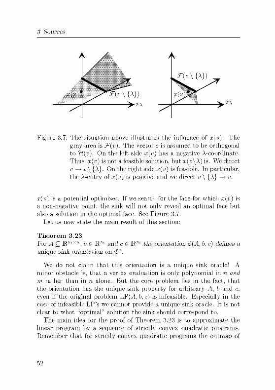
3 Sources
Figure 3.7: The situation above illustrates the influence of x(v). The
gray area is J-'iv). The vector c is assumed to be orthogonalto TLiv). On the left side x(v) has a negative A-coordinate.
Thus, x(-y) is not a feasible solution, but x(v\A) is. We direct
v —> -y\{A}. On the right side x(v) is feasible. In particular,the A-entry of x(v) is positive and we direct v \ {A} —> v.
x(v) is a potential optimizer. If we search for the face for which x(v) is
a non-negative point, the sink will not only reveal an optimal face but
also a solution in the optimal face. See Figure 3.7.
Let us now state the main result of this section:
Theorem 3.23
For A G jRmxn, b G Rm and c G R^
unique sink orientation on £.
the orientation 4>iA, b, c) defines a
We do not claim that this orientation is a unique sink oracle! A
minor obstacle is, that a vertex evaluation is only polynomial in n and
m rather than in n alone. But the core problem lies in the fact, that
the orientation has the unique sink property for arbitrary A, b and c,
even if the original problem LP(A, b, c) is infeasible. Especially in the
case of infeasible LP's we cannot provide a unique sink oracle. It is not
clear to what "optimal" solution the sink should correspond to.
The main idea for the proof of Theorem 3.23 is to approximate the
linear program by a sequence of strictly convex quadratic programs.
Remember that for strictly convex quadratic programs the outmap of
52
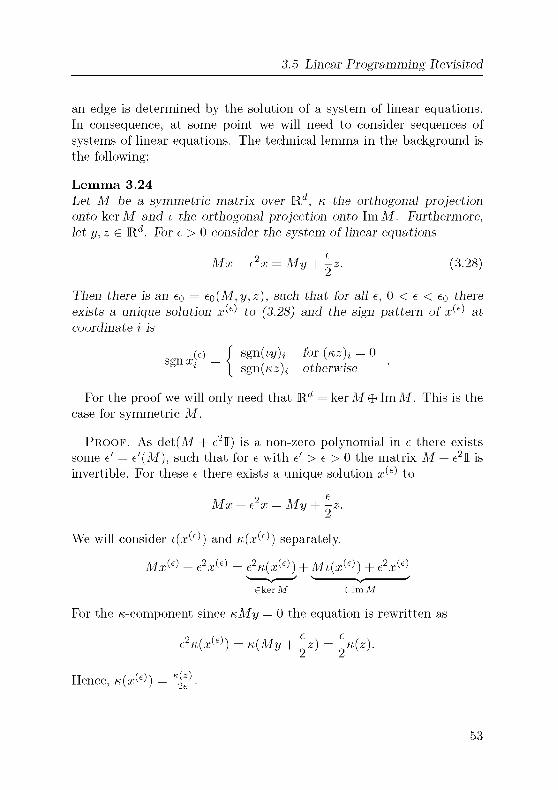
3.5 Linear Programming Revisited
an edge is determined by the solution of a system of linear equations.In consequence, at some point we will need to consider sequences of
systems of linear equations. The technical lemma in the background is
the following:
Lemma 3.24
Let M be a symmetric matrix over Rd, k the orthogonal projectiononto ker M and i the orthogonal projection onto ImM. Furthermore,let y, z G Rd. For e > 0 consider the system of linear equations
Mx + e2x = My+'-z. (3.28)
Tiien there is an eo = eo(M,y,z), such that for all e, 0 < e < eo there
exists a unique solution x^ to (3.28) and the sign pattern of x^ at
coordinate i is
(e)_
/ sgn(w/)j for (kz), = 0sgnx; — -. , -
,, .
* '
sgn(«z)j otherwise
For the proof we will only need that Rd = ker M © Im M. This is the
case for symmetric M.
Proof. As det(M + e2I) is a non-zero polynomial in e there exists
some e' = e'(M), such that for e with e' > e > 0 the matrix M + e2I is
invertible. For these e there exists a unique solution x^ to
Mx + e2x = My+ -z.
We will consider i(x^) and k(x^) separately.
Mx'£> + e2xM^ = e2nix^) + Miix^) + e2x^
GkerM elm M
For the «-component since nMy = 0 the equation is rewritten as
es
e
e2nix^) = KiMy + -z) = -k(z).
Hence, k(x^) = ^-L2e
53

3 Sources
The (,-component case is a bit more involved. The corresponding
equation reads:
Mu{x&) + e2iix^) = u{My + U) = Mu{y) + ^u{z)
(Since u{My) = My = M(«(y) + b{y)) = Mu{y).) Basically, we have the
same equation for i(x^) as before projecting to ImM for x^\ The onlydifference is that now all vectors are in ImM which allows us to invert
M. More precicely, consider the linear functions g : Im M —> Im M,
gix) = Mx and ge : Im M —> Im M, ge(x) = Mx+ e2x. Since ker M and
ImM are orthogonal, g has a trivial kernel. Furthermore, the ge's are
restrictions of bijections. Thus, all maps are invertible. Furthermore,
ge —> g (as elements of the normed algebra of automorphisms on Im M),thus g^1 —> g_1. Applying this convergence to the equation above we
get
ix& = g-\g^))
-+ ff_1(ffWî/))) + o = %).
For a coordinate i G [n] with n{z)l = 0 the sign pattern of xf only
depends on i(x^). Since i(x^) —> i{y) we find an et = et(M,y), such
that for e G (0, et) the point i(x^) has at most distance |(,(y)j|/2 from
(.(y). In particular, sgnx^ = sgm(y)t.For i G [n] with k(z)j / 0 we find an et = e%iM,y,z), such that
for e < e, on the one hand ||t(x^e^) — t(y)|| < \ and on the other hand
l( 2e )*l > *• -^or sucri e the sign pattern of x^ is determined by (-^JOj-Collecting all e4 and e' for eo = min{e', e\,..., e<J the statement of
the lemma holds.
Proof of Theorem 3.23. As already indicated we will reduce the
LP to a sequence of strictly convex quadratic programs. For e > 0 let
Qe = ATA + e2I. This matrix is positive definite since for x G Rn
xTQex = xTATAx + e2xTx = \\Ax\\ + e2\\x\\
54

3 5 Linear Programming Revisited
which is non-negative and equals 0 only for the 0-vector. Therefore, the
function
fe(x) = iAx — b) iAx — b) — ec x + e x x
= xTiATA + e2I)x-i2bTA + cT)x + bTb
is a strictly convex quadratic function. The idea behind fe is that for e —>
0 the part (Ax — 6)T(Ax — b) dominates ecTx and the latter dominates
e2xTx. Thus, minimizing fe over C+ is similar to maximizing cTx over
V. In fact, we will show that for small e the USO defined by fe equals
d>iA,b,c).To distinguish the USO defined by fe and 4>{A, b, c) let us write u -^ v
if u is directed to v according to fe. For u = v \ {A} according to
Theorem 3.20
v\{A}^ev <{=> (i(£)W)a>0
where x^\v) is the unique minimizer of fe over W, i.e., the solution to
Xj = 0 for i ^ v
(V/e(x)), = 0 for*G«.
As the gradient is V/e(x) = 2xT(ATA+e2II)-(25TA+ecT) the equation
system is equivalent to
AlAvx + e2 x = A^b + ^-cv (3.29)
over Mv (where {cv)l = ct for i G v and {cv)l = 0 otherwise).Let M = A^AV, y = x(v) and z = cv. As x^\v) is the solution to
Mx + e2x = My + e/2z, Lemma 3.24 yields some eo = £o(M,y,z) =
eo(A, v, c), such that for e < eo and A G [n] the sign of x^e\v)x is positiveif and only if incv)x > 0, or incv)x = 0 and (lx(v))x > 0.
For the rest of the prove let e < eo. Per definition v \ {A} -^ v if and
only if x^\v)x > 0 for A G v. Hence,
v \ {^} —>t v <^^> i^cv)x > 0 or ((kcv)x = 0 A (lx(v))x > 0).
It remains to show that k(cv) = civ) and l(x(v)) = x(v). Since x(v)is the minimal norm point in TLiv), it is orthogonal to kerÄ^AV, i.e., in
(kerÄ^Ay)1- = lmÄlAv. This establishes t(x(v)) = x(v).
55

3 Sources
For k(cv) = civ) it is enough to show that c — k(cv) is orthogonal to
ker Ä^Ay. In other words, we have to show that for all x G ker Ä^AVthe scalar products (x, c) and (x,k(cv)) are equal. We already know
that (x, cv) = (x, «(c^)} (as k(cv) is the orthogonal projection of cv onto
kerÄ^Ay) and (x, c) = (c,cv) (since cv is the orthogonal projection of
c onto R-" and x G R-"). Hence, the desired equality is shown. D
With Theorem 3.23 we established a reduction from any LP(A, b, c)with n variables and m constraints to a USO of dimension n. Fur¬
thermore, the reduction is polynomial in n and m. But as long as we
cannot relate the sink of the USO to an optimal solution of LP(A, b, c)the reduction is useless.
Proposition 3.25
If the linear program LP (A, b, c) has an optimal solution then it attains
its optimum in x(o) of the unique sink o of 4>{A, b, c).
Proof. If the linear program has an optimal solution the set of all
optimal solutions forms a face T = J-'iv). Let x* be the minimal norm
point in T and o := {A |xA^0}. We prove that o is a (and therefore
the) sink of 4>{A, b, c) and x* = x(o).Since x* G TL(o) n P we are in a feasible vertex. In particular, T{o)
is a nonempty face of V. Furthermore, o G v and in consequence T{o)is a subface of T = J-'iv).
Since x* as an element of R° is strictly positive for small e the pointx* + ecio) is still in T{o). As a point in T{o) G T the objective value
of x* + ecio) equals the value of x*, so
0 = c (x* + tc-io)) — c x* = ec cio) = e||c(o)|| ,
which shows cio) = 0.
We use Lemma 3.14 to show that x* = x(o). Consider the norm
function g : x i—> ||x||. The gradient of g is \7g = 2xT. For x G TL(o) we
thus have to show that 2xT(x — x*) > 0. Since x* is strictly positivein R° and x G R° we find some 9 > 0, such that 6(x — x*) is strictly
positive in R°. This 6(x — x*) is in T{o). In T{o) we know that x* is
minimal norm point. Hence, 2öxT(x — x*) > 0.
In particular, for all A G o we know that cio)x = 0 and x(o)A > 0,
i.e., o \ {A} —> o.
56

3.5 Linear Programming Revisited
It remains to show that for A G [n] \ o we have o U {A} —> o. For this
to happen either c(oU{A})A < 0, or c(oU{A})A = 0 and x(oU{A})A < 0
has to hold. We will rule out all other sign patterns for cio U {A})A and
x(oU{A})A.First assume cio U {A})A > 0. Choose e > 0 small enough, such that
x* + ecio U {A})M is still non-negative for /x G o. For such e the pointx* + ecio U {A}) is in V. Furthermore
cT(x* + ec(oU{A})) = cTx* + ecTc(o U {A})
= cTx* + e||c(oU{A})||2 >cTx*
in contradiction to x* being optimal. Hence, cio U {A})A < 0.
Now assume cio U {A})A = 0 and x(o U {A})A > 0. In this case
cio U {A}) is not only in ker A n R^U^A^ but in ker A n R-". Furthermore,c - cio U {A}) is orthogonal to ker A n R^ as well as to ker A n RoU{A}.
Thus, cio U {A}) = cio) = 0. But then Tip U {A}) is an optimal face,
i.e., subface of F. In particular, x(v U {A}) G TL(o U {A}) Ç TLiv). Since
x* is strictly positive in M,v and we assumed x(o U {A})A > 0, for some
9 G [0,1] the convex combination (1 — 9)x* + 6x(o U {A}) is still non-
negative. Hence, (1 — 6>)x* + 6>x(oU{A}) G T. Furthermore, x(oU{A}) is
of smaller norm than x*, as x* G W(oU{A}) but x\ = 0. In consequence,
by convexity of the norm function (1 — 9)x* + 6x(o U {A}) is a point of
smaller norm than x* in T. This contradicts the choice of x*. D
In contrast to the first reduction from linear programming to USOs in
this more general approach cycles can arise. See for example Figure 3.8.
The LP in Figure 3.8 is highly degenerate since the equation Ax = b
has no positive solution. Ergo all faces are fake. In particular, the cycleis found among the fake faces. So far, no example is known with a cyclein the feasible region.
57

3 Sources
maxxi such that
(-«1 Jdk 47)
Figure 3 8 An LP with a cyclic USO The matrix has full rank Thus,all TLiv) aie points and c(v) = 0 In particular, x(v) alone
decides the orientation The vertices are labeled by their
x(-y) The highlighted edges form a cycle
58

3.6 Remarks
3.6 Remarks
Abstract objective functions were first introduced by Adler and Saigal
[1]. They provide a general framework for the RandomFacet algo¬rithm. How exactly linear programming relates to the larger class of
abstract objective function is unknown up to now. In general, it is hard
to decide whether or not an abstract objective function can be realized
as linear program. The Holt-Klee condition is only a weak indication.
Recently, Develin [8] proved that the number of orientations induced
by linear programs compared to the orientations fulfilling the Holt-Klee
condition is vanishing as the dimension grows. His techniques can be
applied to all reductions to USOs where the orientation is decided ac¬
cording to sign patterns of polynomials. In particular, all reductions in
this thesis are of such type.
The reduction from linear complementarity problems is historicallythe first appearance of unique sink orientations. It was introduced by
Stickney and Watson [40].The concept of strong LP-type problems was introduced by Gärtner
[13, 11] to capture the combinatorial structure of quadratic programs. It
is called strong LP-type problem as by fixing one of the two parameters
one gets an LP-type problem. (For LP-type problems see [15]). The
definition of strong LP-type problems here is slightly more general than
Gartner's approach, as here we allow arbitrary posets (O, <) whereas
originally O = R was assumed.
As it turns out this generalization allows us to capture strictly convex
quadratic programming as strong LP-type problem and thus is the more
natural definition.
The idea to view a linear program as a limit process of strictly convex
programs originates from Gärtner [13]. The reduction presented here is
particularly nice as the resulting USO can be described in terms of the
LP only.The hope is that 4>{A, b, c) can be shown to be USO without the detour
via quadratic programming. In classical LP-theory one tends to assume
that an LP has a unique solution. The orientation 4>{A, b, c) has to deal
with degenerate cases and assigns some solution even to unbounded or
infeasible LP's. The key to fully understand 4>{A, b, c) is a geometricview to these solutions.
59
3 Sources
In the unbounded case 4>{A, b, c) answers a feasible ray as witness for
the unboundedness. Which ray? And how can one distinguish between
infeasible and unbounded cases? Both questions remain unanswered.
60

4 Structure
Viertes Geschoss Hier
wohnt der Architekt Er
geht auf in seinem Plan
Dieses Gebäude steckt
voller Ideen1 Es reicht von
Funda- bis Firmament,
Und vom Fundament bis
zur Firma
(Einsturzende Neubauten)
61
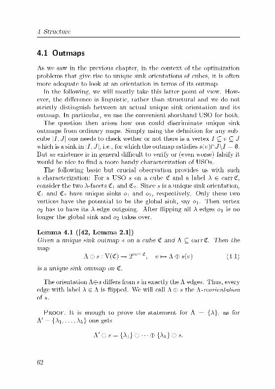
4 Structure
4.1 Outmaps
As we saw in the previous chapter, in the context of the optimization
problems that give rise to unique sink orientations of cubes, it is often
more adequate to look at an orientation in terms of its outmap
In the following, we will mostly take this latter point of view. How¬
ever, the difference is linguistic, rather than structural and we do not
strictly distinguish between an actual unique sink orientation and its
outmap. In particular, we use the convenient shorthand USO for both.
The question then arises how one could discriminate unique sink
outmaps from ordinary maps. Simply using the definition for any sub-
cube [I, J] one needs to check wether or not there is a vertex I Çv G J
which is a sink in [/, J], i.e., for which the outmap satisfies s(-y)n J\I = 0.
But as existence is in general difficult to verify or (even worse) falsify it
would be nice to find a more handy characterization of USOs.
The following basic but crucial observation provides us with such
a characterization: For a USO s on a cube £ and a label A G carr £,consider the two A-facets <t\ and £2. Since s is a unique sink orientation,
£1 and £2 have unique sinks o\ and o2, respectively. Only these two
vertices have the potential to be the global sink, say o\. Then vertex
02 has to have its A-edge outgoing. After flipping all A-edges o\ is no
longer the global sink and 02 takes over.
Lemma 4.1 ([42, Lemma 2.1])Given a unique sink outmap s on a cube £ and A Ç carr £. Tiien the
map
A©s: V(£)^2carr£, v^A®siv) (4.1)
is a unique sink outmap on £.
The orientation A©s differs from s in exactly the A-edges. Thus, every
edge with label A G A is flipped. We will call A © s the A-reorientation
of s.
Proof. It is enough to prove the statement for A = {A}, as for
A' = {Ai,. ..,Afc} one gets
A' © s = {Ai} © • • • © {Afc} © s.
62

4.1 Outmaps
Split £ into the two A-facets <t\ and £2. A subcube £' is either com¬
pletely in one of the A-facets or divided into two faces. For the first
case the orientation in £' is not affected by relabeling A (as £' does not
contain A-edges), and thus has a unique sink.
In the second case [ = £' n £j are facets of £'. Let ot be the sink
of £j. Without loss of generality o\ is the sink of £' with respect to s.
With respect to {A} © s the A-edge in o\ is outgoing, so o\ is no longerthe sink. But now 02 is a sink. All other vertices in £' have an outgoing
edge of label ^ A. Thus, £' has a unique sink. D
As a consequence of Lemma 4.1 an outmap s of a USO is a bijection:For a USO s consider a vertex v G V(£). It has outmap A = s(v). ByLemma 4.1 the map A © s is a unique sink orientation. Its unique sink
is v (as A© s(v) = 0). Hence, in the original s no other vertex can have
the same outmap s(v), i.e., s is injective and therefore bijective.
Corollary 4.2 ([42, Lemma 2.2])A unique sink outmap s on a cube £ is a bijection from V(£) to 2carrc:.
Since a USO induces USOs on all subcubes not only is s bijective but
all its restrictions to subcubes are bijective as well. In particular, for
two vertices u, v their outmap values relative to the smallest subcube
containing u and v differ. The smallest subcube containing u and v
has carrier u © v. The outmap value in u relative to this subcube is
s(u) n (u © v) and the outmap value in v is s(v) P\ (u © v). Hence, in
a USO for each pair of vertices u,v the set (s(u) © s(v)) P\ (u © v) has
to be non-empty. This turns out to be a complete characterization for
unique sink outmaps.
Proposition 4.3 ([42, Lemma 2.3])Given a cube £, a map s : V(£) —> 2carrc: is a unique sink outmap on £
if and only if for all u, v G V(£) we have
{u®v)f\{s{u)®s{v)) ^0. (4.2)
Proof. First assume s has property (4.2) and fix a subcube £[J'J] of
£. We have to show that £[J'J] has a unique sink.
63

4 Structure
Consider the restricted map s : [I, J] —> 2J\I,
s(u) = s(u) n J \ I,
i.e., the outmap of the orientation on [I, J] induced by s. If s is not
injective there are u,v G [I, J], u ^ v, with s(u) = s(v). For these
vertices we get
(s(«)ffisH)nJ\J = l
and since u(Bv G J\I this contradicts the assumption (4.2). Ergo s is
injective, i.e., bijective. In particular there is exactly one sink o G [I, J].Now assume s does not have the property (4.2) and let u,v witness
its failure. But then, since (u © v) n (s(u) © s(v)) = 0, in the subcube
[u n v, u U v] both m and v have the same outmap A = s(u) P\ (u © v) =
s(v) n (u © w). Thus, A © s has two sinks in [u P\ v, u U -y], i.e., is not a
USO. By Lemma 4.1 s is not a USO either. D
Given a cube £ and a G V(£) consider the map
©0 :V(£)^2carr£, v^v®a.
By (4.2) ©a is a USO. In a vertex v an edge is outgoing if the Hamming-distance to a is decreasing along this edge. The orientation ©a is called
uniform orientation towards a. See Figure 4.1 for an example of a
uniform orientation.
A uniform orientation is fully described by a and carr £. Furthermore,
up to isomorphism there is exactly one d-dimensional uniform orienta¬
tions: The map ©a itself is an isomorphism between the cube £ with
the orientation £a and the cube 2carrc: with the orientation id = ©0.Whenever we write the uniform orientation we refer to ©0.
Using uniform orientations one can nicely write down isomorphismsbetween USOs. Let si and S2 be two USOs on <t\ and £2, respectively.A (digraph-)isomorphism ty : V(£i) —> V(£2) has to map the sink o\ of
s\ to the sink 02 of s2. Furthermore, the neighbors o\ © {A}, A G carr £1
map to neighbors 02 © {/«}, /x G carr £2. Thus, ^ induces a bijectiont : carr£i —> carr£2 with *(oi © {A}) = o2 © {t(A)}. But then for
A Ç carr £1 the equation
*(oi © A) = o2©t[A]
64

4 1 Outmaps
Figure 4 1 A uniform orientation The vertices are labeled by their
Hamming-distance to the sink
holds Here t[A] = {t(A) | A g A} is the image of A under t
As ty is a digraph-isomorphism the edge {o\ © A, o\ © A © {A}} m £i
and its corresponding edge {02 © t[A], o2 © t[A] © {t(A)}} are oriented
the same way For the outmaps this implies
t[si(oi© A)] = s2(o2©t[A])
On the other hand, if we find such a t the corresponding ty is a digraph-
isomorphism
Lemma 4.4
Two outmaps s^ on £1 and s2 on £2 describe isomorphic orientations
if and only if there exist a\ G V(£i), 02 G V(£2) and a bijection t
carr £1 —> carr £2, such that for all v G V(£i)
r[si(w©ai)] = s2(-r[?;]ea2) (4 3)
Given two isomorphic USOs si and s2, we can rewrite the above
equation, such that S2 is expressed in terms of si Set a = r[ai] © 0,2
Then for all v G V(£2) we have s2(v) = t[si(t_1[w © a])] If we denote
the image-map A i-> t[A] by t' then
s2 = t'osi o (t')_1 o©0
65

4 Structure
Given a USO s on £d the set of isomorphic USOs on £d has at least
2d members. Let o be the sink of s and a G V(£d). The map s o ©a
has its sink in o © a. Furthermore, as there are d\ possible choices for t
there are at most 2dd\ isomorphic USOs. Both upper and lower bound
are tight.
4.2 Algebraic Excursion
In the following we will mainly consider USOs on the standard cube 2^1,since an arbitrary cube £ is isomorphic to 2ldlmC-l. By Corollary 4.2 a
USO s on £d is a permutation of 2^1. The inverse s_1 is a map from
2carrl£d = y^d) tQ y^d) = 2carr<td
_por „^^ g 2^ and ^ = s(^) We
get
(#i © £2) n (s_1(£i) © s_1({i2)) = (s(^i) © s(v2)) n («i © w2) ^ 0.
Hence, s_1 satisfies (4.2) and thus is a USO. This suggests to study the
set of all USOs on £d
USO(d) = Is : 2[d] —> 2[d] s is a unique sink orientation | (4.4)
as a subset of the symmetric group S2[d\. In particular, one might ask
how USOs behave under the group operation o on the symmetric group.
We will study the following two questions:
1. Which subgroups of S2[d\ operate on USO(d)?
2. What is the subgroup generated by USO(cf)?
An easy example regarding the first question is given by the subgroup
({©a I a G 2^ } , o) = (2^, ©). This group operates on USO(d) from
the left as well as from the right: for any s G USO(d) the maps s o ©a
and ffia os are USOs (which is a direct consequence of (4.2)). Both maps
we already saw, s o ©a is the isomorphic image of s with sink in o © a
(where o is the sink of s). And ©a o s = a © s is the a-reorientation of
s. Figure 4.2 shows how both operations perform on a USO.
Except for this rather simple group (and its subgroups) no other group
operates on USO(d).
66

4 2 Algebraic Excursion
Figure 4 2 A USO s (in the middle), so©^ 2} (left) and ©{i 2} °« The
left orientation is the mirror image of the middle one alongthe gray axis In the right orientation the flipped edges are
highlighted
Proposition 4.5
For a map g 2^1 —> 2^1 the following statements are equivalent
(l) g = ©a for some a G [d],
(u) for all unique sink orientations s, so g is a unique sink orientation
and
(in) for all unique sink orientations s, gos is a unique sink orientation
Proof We just argued that s o ©a and ©a o s is a USO for all USOs
s and all a This establishes (i)=>(n) and (i)=>(m)In the following we proof (n)=>(i) and then (m)=>(i) using (n)=>(i)
By Corollary 4 2, g has to be a bijection for (n) or (m) to hold For
(n)=>(i) we argue that for any u G V(£) the set <;_1(w) © <7_1(0) equalsu In fact, the mam ingredient is that u Ç. g-1 (u) ® <;_1(0)Assume s o g is a USO for all USOs s Fix u G [d] For A G m choose
a USO s = su x, such that s(u) = {A} and s(0) = 0 Such an s reveals
Aej-'Wer1^)
0 ¥= isogig-\u))®Sogig-\%)^ig-\u)®g-1^))= isiu)®Si%))r\ig-\u)®g-\%))= {A}nig-1iu)®g-1i9))
67

4 Structure
If we find su A for all A G u, we get u G g 1(m) © g 1(0) Such su A
exists, e g
/ \_ / v x£vSuX[V)
\ v®iu\{A}) Aev'
is USO, as one can easily verify by checking the USO-property
Thus, the mapping h w i—> <?_1(w) © <7_1(0) is bijective and for all
u G V(£) we have u G h(u) By induction on |w| we can conclude that
u and <;_1(w) © <7_1(0) have to be equal Hence
g~ = ©s i(0)
and g = g^1 This proves (n)=>(i)For (m)=>(i) observe that if g o s is a USO then s-1 o g^1 is a USO
In particular, if (m) holds for a map g, then (u) holds for g^1 Since
we already know that (u) implies (l), we find an a with g^1 = ®a But
then g = g-1 = ®a
The answer for the second question is that the smallest group con¬
taining USO(d) is the symmetric group Even worse, already the trans¬
positions in USO(d) generate S2[d\
Proposition 4.6
The group generated by all d-dimensional unique sink outmaps is the
symmetric group S2[d\
Proof As a first step we characterize the transpositions of S2[d\which are also in USO(d) For a Ç [d] and A G [d] consider the uniform
orientation towards 0 and in this orientation flip the edge between a and
a©{A} In every vertex v G [d], v ^ a, a©{A} the corresponding outmapis still s(v) = v The outmap value of a in the uniform orientation
is a, now since the A-edge changed, it is sia) = a © {A} Similarly,
sia © {A}) = a Therefore, s is the transposition that exchanges a and
a © {A} We will prove that this is the only type of transposition in
USO(d)Consider a transposition s = (a, 6) G S2[d\ Then for all u, v G 2^d\
u, v ^ {a, 6} (4 2) is satisfied trivially and so is for the pair a, b Only the
68
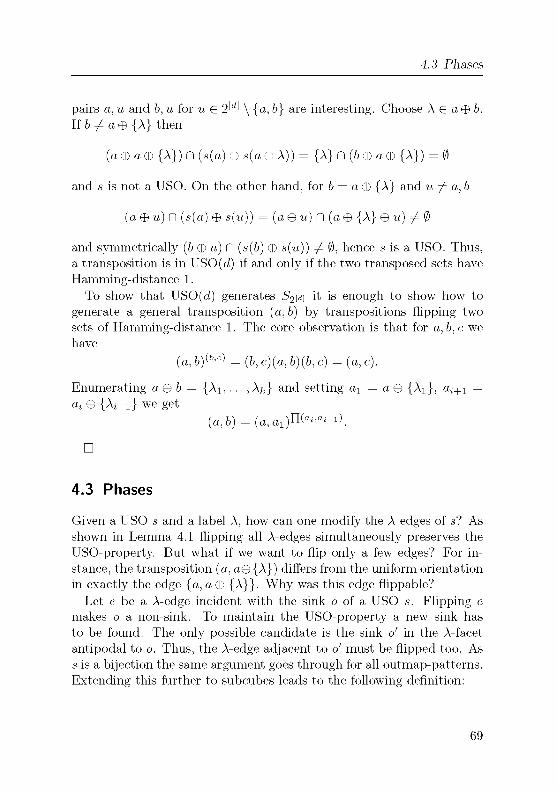
4.3 Phases
pairs a, u and b, m for m G 2^1 \ {a, 6} are interesting. Choose A G a © 6.
If b ^ a © {A} then
(a © a © {A}) n isia) ® sia ® A)) = {A} D (6 © a © {A}) = 0
and s is not a USO. On the other hand, for b = a © {A} and u^ a,b
(a © w) n (s(a) © s(w)) = (a © w) n (a © {A} © u) ^ 0
and symmetrically (6 © w) n (s(6) © s(w)) 7^ 0, hence s is a USO. Thus,a transposition is in USO(d) if and only if the two transposed sets have
Hamming-distance 1.
To show that USO(d) generates S2[d\ it is enough to show how to
generate a general transposition (a, b) by transpositions flipping two
sets of Hamming-distance 1. The core observation is that for a, b, c we
have
(a, 6)(6'c) = (6, c)ia, b)(b, c) = (a, c).
Enumerating a © b = {Ai,..., A^} and setting ai = a ® {Ai}, al+i =
at © {Aj+i} we get
(a,6) = (a,a!)n(a-^+i).
D
4.3 Phases
Given a USO s and a label A, how can one modify the A-edges of s? As
shown in Lemma 4.1 flipping all A-edges simultaneously preserves the
USO-property. But what if we want to flip only a few edges? For in¬
stance, the transposition (a, a©{A}) differs from the uniform orientation
in exactly the edge {a, a © {A}}. Why was this edge flippable?
Let e be a A-edge incident with the sink o of a USO s. Flipping e
makes o a non-sink. To maintain the USO-property a new sink has
to be found. The only possible candidate is the sink o' in the A-facet
antipodal to o. Thus, the A-edge adjacent to o' must be flipped too. As
s is a bijection the same argument goes through for all outmap-patterns.
Extending this further to subcubes leads to the following definition:
69

4 Structure
Figure 4 3 A USO and its phases Edges m phase are connected by a
shaded line
Definition 4.7
Let s be a unique sink orientation of dimension d and A G [d] Two
A-edges e\ and e2 are m direct phase (which we denote by e\ \\ 02) if
there are v\ G e\, v2 G e2, such that
iv-i ® v2) D isiv-i) ® siv2)) = {A} (4 5)
Let ei and e2 be two A-edges m direct phase In particular, for the
witnesses v\ G e\ and V2 G &2 the label A has to be m v\ ® V2 Hence,
v\ and V2 are m different A-facets Furthermore,ei and &2 have to be
directed towards the same A-facet Since A G s{v\)@s(v2), say A G s(v\),the edge e\ is leaving v\, 1 e
, pointing towards the A-facet containing
V2 The edge &2 is entering V2, 1 e,also pointing towards this facet See
Figure 4 3 for an exampleConsider a USO s with A-edges e\ and &2 m direct phase Let v\ G e\
and V2 G 2 witness that they are in phase If one flips e\ but not &2
the resulting orientation s' has a new outmap s'(vi) = s(vi) © {A} in v\
whereas in V2 nothing changed, 1 e, s'(v2) = s(v2) But then
(«1 © v2) n is'ivi) © s'(v2)) = iv! © v2) n (s(«i) © s(v2)) © {A} = 0
and s' is not a USO
70
4 3 Phases
In consequence, to preserve the USO-property one has to flip edgesin phase simultaneously As an edge is directly in phase with itself
and being directly in phase is symmetric, the transitive closure is an
equivalence relation
Definition 4.8
Given a unique sink orientation s, let ||| be the transitive closure of ||The phase of an edge e is the set of all edges m phase to e, {e' | e ||| e'}A phase of A-edges is called a A-phase
As HI is an equivalence relation the set of edges is partitioned into
phases Every phase is a A-phase for some A since edges m phase are of
the same label
Proposition 4.9
Let L be a set of non-adjacent edges m a unique sink orientation s The
orientation s' one obtains by flipping all edges m L is a unique sink
orientation if and only if L is a union of phases
Proof The set L is a union of phases if and only if it is closed under
First assume L is closed under ||| We will verify that s' is a USO
by checking (4 2), l e,for pairs u, v of vertices we show that the set
(w © v) n (s'(w) © s'(v)) is not empty The sets s'(w) and s(w) differ at
most m one element as u is incident to at most one edge m L
If neither of u and v are incident to edges m L, s(w) = s'(w) and
s(w) = s'iv) and there is nothing to prove
If exactly one of the vertices is incident to an edge m L, say e =
{u, m©{A}} G L, then s'(w) = s(w)©{A} and s'iv) = s(w) Furthermore,since the A-edge m v is not in L, the two edges e and {v, v © {A}} are
not in A-phase In particular, (u © v) n (s(u) © s(v)) ^ {A} Hence,
(u ® v) n (s'(u) © s'iv)) is not empty
If u and v are both incident to A-edges in L we flip both edges That
is, s'(u) ® s'iv) = (s(w) © {A}) © (s(v) ® {A}) = s(u) ® s(v) and this case
is also good
Finally, consider two vertices u and v incident to edges in L of different
label, say e„ = {u, u© {A}}, ev = {v, v© {/x}} G L If {A, ^}C\u®v = 0,
71

4 Structure
the values (w © v) n (s(u) © s(v)) and (m © w) n (s'(w) © s'iv)) are equal,hence nonempty.
For A G u © v and /x ^ m © v the edge e„ and the A-edges incident
to v cannot be in phase. If they were, the A-edge incident to v would
be in L. But then L would contain two adjacent edges. Thus, the set
(u © v) n (s(u) © s(v)) contains a label different from A. This label is
also in the set (u®v) P\ (s'(u) © s'iv)). The case A ^ u®v and /x G u®v
is resolved symmetrically.If A, /x G m © w consider the vertex w in [w n w, u U w] with outmap
s(w) C\ iu ® v) = (s(u) © {A}) n (u © w). Such a vertex exists since s
induces a bijection on [uP\v,uL)v]. The A-edge incident to w is in phasewith e„.
Assume (w © -y) n (s'(u) © s'(w)) = 0. This can happen only if the set
(u © v) n (s(w) © s(w)) is equal to {A, /j,}. But then the /x-edge incident
to w is in phase to ev with respect to s. This cannot be since then both
the A- and the /x-edge incident to w would be in L.
For the back-direction assume L is not closed under |||. We will show
that then s' is not a USO. In this case one finds edges e and e' being in
phase and e G L but e' ^ L. As ||| is the transitive closure of || we find
a sequence of edges e\, e2,..., e^ with
e = ei || e2 || •• • || efc = e'.
Along this sequence at some point we will leave L, i.e., for some i the
edge et is in L but el+i is not. Let vt G e4 and vl+\ G eî+i witness
e4 || et+i. Then («j © vt+i) n (s(wj) © s(wî+i)) = {A}. Since e, £ L we
have s'ivt) = s(vt) © {A} and since el+i ^ L the outmap values s'(vl+i)and s(wj+i) agree. But then («j © vl+\) n (s'(wj) © s'(-yî+i)) is empty,
i.e., s' is not USO. D
In the uniform orientation every edge is only in phase to itself. If one
chooses two edges incident to the sink then flipping the edges in L gives
a 2-face with two sinks. This shows that we cannot drop the condition
that L contain only non-adjacent edges.The simplest way to find a set L without adjacent edges is to take only
edges of the same label. In particular, Proposition 4.9 is applicable to
the set of all A-edges. Thus, Lemma 4.1 can be seen as a simple corollaryof Proposition 4.9. (We heavily used Proposition 4.3, i.e., Lemma 4.1
72
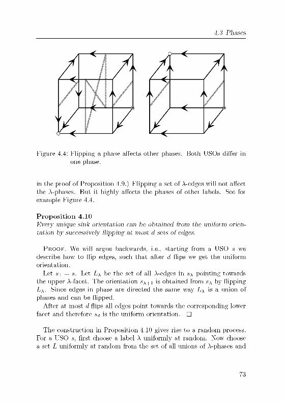
4 3 Phases
Figure 4 4 Flipping a phase affects other phases Both USOs differ in
one phase
in the proof of Proposition 4 9 ) Flipping a set of A-edges will not affect
the A-phases But it highly affects the phases of other labels See for
example Figure 4 4
Proposition 4.10
Every unique sink orientation can be obtained from the uniform orien¬
tation by successively flipping at most d sets of edges
Proof We will argue backwards, î e, starting from a USO s we
describe how to flip edges, such that after d flips we get the uniform
orientation
Let s i= s Let LA be the set of all A-edges in sA pointing towards
the upper A-facet The orientation sA+i is obtained from sA by flipping
Lx Since edges in phase are directed the same way LA is a union of
phases and can be flippedAfter at most d flips all edges point towards the corresponding lower
facet and therefore Sd is the uniform orientation D
The construction in Proposition 4 10 gives rise to a random process
For a USO s, first choose a label A uniformly at random Now choose
a set L uniformly at random from the set of all unions of A-phases and
73
4 Structure
flip L. Call this USO sr,. As sr, differs from s exactly in the edges in L,the A-phases of s and sr, agree and (sl)l = s.
For a d-dimensional USO s let phA(s) be the number of A-phases.The above random process is described by the following transition-
probability:
1 f EA=i2~phA(s) for s = s'
Ps,s> = -, \ 2~ph^s) for s' = sL, L collection of A-phases
[ 0 otherwise
(4.6)The set L is the unique set of edges in which s and s' differ and therefore
pSis' is well-defined. These probabilities define a Markov chain.
We recall the definition of a Markov chain. For a detailed discussion
see [5]. Let iXt)teN be a random process, i.e., a sequence of random
variables. For the sake of simplicity we assume that the range of all Xt is
finite. We interpret t as time and Xt as a random experiment conducted
at time t. Suppose now that the experiments at time 0,..., r — 1 have
been conducted with outcomes Xq = xn, ...,Xt-\ = xt-\. These events
may influence the next experiment, i.e., for each possible outcome xt,
the probability
Pr[Xt = xt | X0 = x0, Xi = xi,..., Xt-i = xt-i]
may depend heavily on the past results xn,..., xt-\.
The random process (Xt)teN is called a Markov chain if the outcome
only depends on the last result, i.e.,
Pr[Xt = xt | X0 = x0, ,Xt-i = xt-i = Pr[Xt = xt | Xt-i = xt-i]
for all t and all xn, x\,..., xt. A Markov chain is homogeneous if all Xthave the same range of positive values and for all x, y the probabilities
Pr[Xt = x | Xt-i = y] do not depend on t. For a homogeneous Markov
chain the (common) range is called the state space and its elements are
the states of the Markov chain. Furthermore, a homogeneous Markov
chain is fully described by its state space, the transition probabilities
Px,y = Pr[Xt = y | Xt-i = x],
and Pr[Xo = x\.
74

4 3 Phases
The mam fact we are interested in, is that a Markov chain can simu¬
late the uniform distribution For this we need three more definitions
Consider the digraph G on all possible states of the Markov chain A
state x has a directed edge to y if the transition probability px y> 0
The Markov chain is called symmetric if px y= py x
for all states x and
y The chain is irreducible, if the digraph G is strongly connected, l e,
for all states x and y we find directed paths from x to y and from y to
x Finally, the chain is aperiodic if we do not find a state x and A; G IN,k > 1, for which all cycles in G containing x have length congruent to 0
modulo k
A Markov chain is said to converge to the uniform distribution on
the state space S if the k-th powers of the transition matrix (px y)x yes
converges to (l/^D^ yes In other words, a Markov chain converges
to the uniform distributions if the outcome of an experiment is nearlyuniform distributed over S as t —> oo For aperiodic, symmetric and
irreducible homogeneous Markov chains the following is known
Theorem 4.11
Any aperiodic, symmetric and irreducible homogeneous Markov chain
converges to the uniform distribution on the state space
A Markov chain is aperiodic if every px x > 0 Furthermore, for
symmetric Markov chains the digraph G can be simplified to a graphand strongly connected can be replaced by connected
Applied to the situation of d-dimensional USOs the Markov chain
described in (4 6) is a random walk on the graph Gd with
V(Gd) = USO(d) and {su s2} G E(Gd) <{=> pSl S2> 0 (4 7)
Proposition 4.12 ([30])The homogeneous Markov chain defined by the transition probability m
(4 6) is aperiodic, symmetric and irreducible
Proof As ps s> 0 the Markov chain is aperiodic
For symmetry let s ^ s' be two USOs and L the set of edges in which s
and s' differ If L contains edges of different labels then ps si= 0 = psi s
since flipping only edges of one label will not destroy all differences in
L For the case that L consists only of A-edges L has to be a collection
75

4 Structure
of A-phases, since flipping all edges in L transforms s into s' and s' into
s. Furthermore, as flipping one A-phase does not change the set of all
A-phases the numbers phA(s) and phA(s') agree. Thus, pSiS/ = ps/iS.
By Proposition 4.10, there is a flip-sequence transforming a given USO
s to the uniform USO. Each flip in the sequence has positive probability.
Thus, there is a path in Gd from s to the uniform USO. Hence, Gd is
connected. Since the Markov chain is symmetric this implies that the
chain is irreducible. D
In a more concrete form Proposition 4.12 says that we can generate a
random USO (drawn uniformly at random from USO(d)) the following
way: Choose an arbitrary d-dimensional USO. Then repeatedly choose
a random A together with a random set of A-phases and flip this set.
After some while the resulting orientation will be "sufficiently random".
The core problem here is that we do not know how often we need to
repeat. So far, we have not been able to resolve this problem.Nevertheless in the following we start a discussion about the graph
Gd- The results we are able to achieve are a (weak) indication that
the Markov chain has a reasonable mixing rate. The diameter of Gd
is at most 2d by Proposition 4.10. Furthermore, we will show that its
connectivity is not too small. Obviously, Gd is closely related to the
numbers phA(s).The easiest example for a d-dimensional USO with exactly one d-phase
is the following: take some (d— l)-dimensional USO s and s = ffi[d_i] osthe orientation differing from s in every edge. Then there are only two
USOs having s in the lower d-facet and s in the upper d-facet, namelythe one with all d-edges directed downwards and the one with all d-edgesdirected upwards. If there were two d-edges with different orientation,there would be a 2-face containing a d-edge pointing upwards and a dr¬
edge pointing downwards. In this 2-face the other two edges would be
in phase, but s and s differ in them.
Similarly, to have 2d_1 d-phases we take some (d — l)-dimensionalUSO and place a copy of it in the lower and upper d-facet of a d-cube.
Then the d-edges in this d-cube can be directed arbitrarily. This is the
only construction achieving 2d_1 d-phases. Call an edge which is in
phase with no other edge flippable. The next lemma shows that an edgee is flippable if and only if the outmaps of the two incident vertices differ
76

4 3 Phases
in the label of e only Consequently, if all d-edges are flippable we must
have the same orientation in the upper and lower d-facet
Lemma 4.13
For a unique sink outmap s an edge {v,v © {A}} is m phase with no
other edge if and only if
siv®{A}) = siv)®{A}
Proof If {v, v © {A}} is only in phase with itself, then in particularno vertex other than v © {A} has the outmap value s(v) © {A} (Oth¬erwise, this vertex would be in phase with v) But since s is a bijectionv © {A} takes the value s(v) © {A}Now if there is an edge in phase with {v,v © {A}} there has to be a
vertex v' with (v ® v') n (s(v) ® s(v')) = {A} Thus
(v ® {A} ® v') n (s(v) ® {A} ® s(v')) = 0,
and s is not a USO D
Let us now consider the overall number of phases of a USO s, l e,
ph(s) = J2xe\d] Ph\(s) By the observations above ph(s) is bounded
from below by d and from above by d2d_1 The upper bound cannot be
improved, since by Lemma 4 13, in the uniform orientation every edge is
flippable In dimension 2 the eye has 4 phases and the bow has 3 phasesIn particular, the lower bound of d is not tight even in dimension 2
Lemma 4.14
For d > 2 a d-dimensional unique sink orientation has at least 2d phases
Proof Let s be a counterexample of minimal dimension d > 2
More precisely, s is a d-dimensional USO with less than 2d phases and,if d > 3, all USOs of dimension d — 1 have at least 2d — 2 phases
In particular, we find a label A for which s has only one A-phase For
this A all edges have to be directed towards the same A-facet (as they are
in phase) Now consider two /x-edges e\ and e2, /x ^ A, in the different
A-facets Assume e\ and &2 are in phase The witnessing vertices v\ and
V2 then agree in the orientation of their incident A-edge Hence, one of
77

4 Structure
the A-edges points towards the upper A-facet, whereas the other points
towards the lower A-facet But then there is more than one A-phaseIn other words, for such s we have one A-phase and all other phases
are phases of one of the A-facet For the overall number of phases we
therefore can count the number of phases in the lower and in the upper
A-facet independentlyFor d = 3 both A-facets have at least 3 phases Hence, the number
of phases in s is at least 3 + 3+l = 7> 2d, which contradicts the
assumption
For d > 3, by assumption the two A-facets have 2d — 2 phases each
Altogether this would give 2d— 2 +2d — 2 + 1 = 4d — 3 > 2d phases for
s, a contradiction D
The numbers phA(s) are closely related to the degree of s in the graph
Gd defined in (4 7) The A-edges of s can be oriented in 2ph^s) ways
One of the orientations is s itself, the others are neighbors in Gd Hence,the degree of s in Gd is
deg(s) = J2 2PhA(s) " 1
xe[d]
Let ph(d) = mm {ph(s) | s G USO(d) } In terms of ph(d) Lemma 4 14
proves 2d < ph(d) We will now relate ph(d) to the minimal degree (5(d)of Gd
Lemma 4.15
dr2pHd)/d _ 1) < Sid) < 2PhW - 1
Thus, by Lemma 4 14 the minimal degree of Gd has to be at least
d(22d/d - 1) = 3d
Proof First consider a USO s which is tight in the number of
phases For this s we get
Yl Phx(s) = Ph«>
xe[d]
J2 2ph^s) - 1 > (5(d)
xe[d]
78

4.3 Phases
Without knowing how ph(d) distributes over all labels, we want to
bound the latter sum from above. In general, the following holds:
E2fc* k% d_ o, y^
fej K )K
We prove this by induction on d. The statement is clearly true for d = 1.
Now assume it is true for d—1. Then for a fix kd the sum X^eW-H 2fc* —1
has maximal value 2K~kd — 1. Thus, we need to maximize the function
kd <-^ 2K~kd — 1 + 2kd over 0 < kd < K. The maximum is attained at
kd = 0. Applied to our situation this proves the upper bound on (5(d).For the lower bound on (5(d) consider a USO s' with minimal degree
in Gd- For such s' we know
J2 2PhA(s') _ 1 = Sid)
]TphA(S') > ph(d).
xe
xel
Again we prove a upper bound for the latter sum:
5>*e
kt>0,J22K -l=L\ = dlogiL + d) - dlog d.
te
The statement is true for d = 1. Now fix kd and assume the statement
is true for d — 1. Thus, we aim to maximize
kd » kd + id - 1) log(L - 2kd + 1 + d - 1) - id - 1) log(d - 1).
The first derivative of this function is kd i—> 1 — (d— l)2fcd(L — 2kd +d)_1,which is 0 for kd = log(L + d) — log d. In fact, this is the maximum for
kd > 0 and for this value of kd we get
A;d+(d-l)log(L-2fcd + l+d-l)-(d-l)log(d-l) = dlog(L+d)-dlogd.
D
79
4 Structure
The (edge-)connectivity of Gd is trivially bounded by (5(d) from above
For a lower bound the number ph(d) is of much more use
Lemma 4.16
The graph Gd is 2(d + l)-connected for d > 2
Proof Since there are 2d uniform orientations, after deleting 2d+ 1
orientations there is still one uniform orientation left Without loss of
generality, it is the orientation towards the empty set We will show
that even if 2d + 1 USOs are forbidden we can find a path from a given
USO to the uniform orientation For the rest of the proof fix a USO s
We want to successively comb edges until everything is uniform De¬
fine for a label A the set
Lx = {{v, v U {A}} | A £ v, v - v U {A} } ,
which is the set of all A-edges differing from the uniform orientation
Along a path we want more and more labels to agree with the uniform
orientation, l e,LA = 0 for progressively more labels A Call such A
combed (as all edges are "combed downwards") Let k be the number
of combed labels, l e,without loss of generality L\, ,Lj. are empty
The goal is to comb one more label (and then proceed inductively)One way to achieve this is to flip a LA The resulting orientation sA is
combed ml, ,k and A (As already argued, LA is closed under phasesand therefore flippable )
For k = d—1, flipping Ld will end in the uniform orientation (which by
assumption has not been deleted) For the rest of the proof let k < d — 1
and assume that for k + 1 there is a path to the uniform orientation In
particular, it is enough to show that there is a path from s to a USO
with k + 1 combed labels
Every sA, A G {k + 1, , d} is combed in k + 1 labels and connected
to s by an edge Thus, if we can choose one of these orientations we are
done For the rest of the proof assume that all these d — k direct pathsvia the sA's are deleted
We proceed in an indirect way First we move"
horizontally" to a new
USO with k combed labels and from there "
go up" to a USO with k+1
combed labels If we find more than d — k + 1 such detours not all of
them can be blocked
80

4 4 Local Changes
Decompose s into 2k subcubes 0 0* * to 1 1* * As s is
combed in the labels 1, ,k no two edges in different subcubes can be
directly in A-phase, A = k +1, ,d (The outmap values of the incident
vertices differ at least in one of the labels 1, ,k) For k < d — 2,Lemma 4 14 applied to each subcube yields 2(d — k) phases per subcube
For k = d— 2 the subcubes are 2-dimensional and have at least 3 phases
Hence, the {k + 1, , d}-edges split into at least 2fc2(d — k) phases for
k < d - 2 and 3 2d-2 fork = d-2
The first term 2fc2(d — k) is at least 2d if and only if d > k2£_1 or
k = 0, which is the case for k < d — 2 The second term 3 2d_1 is at
least 2d for d > 2 In particular, the {k + 1, , d}-edges partition into
at least 2d phases For such a phase P define P If P ^ Lx set P = P
otherwise let P be the set of all A-edges By this choice no two P are
equal and all P can be flipped without ending in an sA
For any such P one can first flip P Choose afterwards some A G
{k + 1, ,d} different from the edge-labels in P and flip LA This
results in a USO sp which has k + 1 combed edges
Altogether there are d — k direct routes via sA 's and at least 2d routes
via sp's Hence, one has to delete 2d® d — k > 2d + d — d + 2 = 2d+2
vertices from G to kill all these routes In particular, G is still connected
if one deletes only 2d + 1 vertices D
Virtually the same arguments go through for all bounds /(d) < ph(d),as long as /(d) has the following property
In particular, every polynomial lower bound on ph(d) yields a polyno¬mial bound on the connectivity
4.4 Local Changes
To be in phase is more a global than a local property Even edgeswhich are far away potentially can be in the same phase This makes
the concept hard to handle in general In contrast, it can be decided
locally whether a given edge is in phase with any other edges at all byLemma 4 13 In the following we want to generalize Lemma 4 13
81

4 Structure
Figure 4.5: A USO with a hypersink (marked with hs) and a hypervertex
(marked with hv).
According to Lemma 4.13 an edge {o, o©{A}} in the sink o is flippableif and only if sio © A) = sio) © {A} = {A}. In other words, the 1-
dimensional subcube {o, o © {A}} is flippable if and only if all edgesincident to (a vertex of) the subcube are incoming.
Definition 4.17
For a cube £ and a subcube £o an edge {u,v} is called incident to
£o if u G V(£o) and v ^ V(£o). The subcube £o is a hypersink in a
unique sink orientation s if all incident edges are incoming, i.e., directed
towards the vertex in q. It is a hypervertex if there is a A G carr£o,such that £o is a hypersink in A® s.
In other words, for a USO s on a cube £ a subcube £o is a hypervertexif and only if all incident edges of the same label are oriented the same
way. For an example see Figure 4.5. With this new notation Lemma 4.13
claims that every 1-dimensional hypervertex can be oriented arbitrarily.
Lemma 4.18 ([39, Lemma 3])Let s be a unique sink outmap on a cube £ and £q be a hypersink. For
82
4 4 Local Changes
a unique sink outmap so on £o, dehne s' V(£) —> 2carrc: by
,_
f s(«) for « £ V(£0)1 J
\ soH for«GV(£0)
Then s' is a unique sink outmap on £ Furthermore, if s and so are
acyclic then s' is acyclic
Proof The map s' is well defined since carr £o Ç carr £ Further¬
more, since an edge incident to £o is directed towards £o the outmap s'
orients every edge only once
If a subcube £' is a subcube of £o then its orientation is determined
by so As so is a USO there is a unique sink m £' If £' is disjoint from
£o the orientation is determined by s and again there is a unique sink
Now assume V = V(£') n V(£0j) ^ 0 and £' is not a subcube of £0
Then V spans a subcube £0 m £' With respect to s the unique sink of
£' has to be m £0 as £0 is a hypersink For s' the vertices outside V
do not change their outmap In particular, if £' has a sink with respect
to s' it lies m £0 As s' on £0 is given by so and so is a USO there is
exactly one unique sink m £0 which is then the unique sink m £'
Now let s and so be acyclic No directed path m £ can leave £o
Therefore, a potential cycle of s' is contained either m £ and therefore
is a cycle w r t so or m £ \ £o, m which case it is a cycle w r t s
Consequently, if so and s are acyclic, s' is acyclic as well D
At first sight it seems that Lemma 4 13 is of more generality than
Lemma 4 18 as we could apply it not only to 1-dimensional hypersmksbut to all 1-dimensional hypervertices By the definition of a hyperver¬tex it is rather obvious how to extend Lemma 4 18
Corollary 4.19 ([39, Corollary 6])Let s be a unique sink outmap on a cube £, £o a hypervertex of s and
so a unique sink orientation on £o Let A be the set of labels of edges
leaving £o Then the orientation
,( s(v) for^V(£0)
y ' \ s0(t>)UA forve V(£0)
is a unique sink orientation
83

4 Structure
Proof The label set A equals s(-y) \carr£o for any v in £o Consider
s = A© s In s the subcube £o is a hypersink and by Lemma 4 18 can be
replaced by so Call the resulting USO s' Finally, the USO s' = A © s'
has outmap s'iv) = A© A© s(v) for v e-V(£0) and s'iv) = A® s0(v) =
AUsoiv) for v G V(£)oBy Lemma 4 18 one can replace A © s in £o by A © so Relabeling the
resulting USO with A yields s' D
Unlike in Lemma 4 18, here acyclicity does not necessarily carry over
to s' Only in a hypersource the arguments for acyclicity go through as
well
Furthermore, Corollary 4 19 is best possible in the following sense
Assume that for a USO s, a subcube £o and a label A ^ carr£o, the
A-edges incident to £o are not homogeneously oriented, in particular, we
find two neighboring edges {u, u © {A}} and {u © {/x}, u © {A, /x}} with
opposite orientation Then the edges {u,u © {/x}} has to be directed
towards the same facet as {u © {A}, m © {A,/x}} In particular, the
orientation in £o cannot be chosen arbitrarily
4.5 Products
So far, we have discussed ways to modify a USO In the following section
we describe how to generate new USOs from smaller ones Given 2dl
USOs of dimension d2 the idea is to combine these to a {d\ + d2)-dimensional USO In other words, given a di-dimensional USO we want
to blow up the vertices to d2-dimensional subcubes
For cubes such a product is easily defined For two cubes <t\ and
£2 with disjoint label sets the set {»Uji | u g V(£2), v G V(£2)} is the
vertex set of a cube with label set carr £1 U carr £2 Call this cube
£1 x£2
Lemma 4.20 ([39, Lemma 5])Let £p and £# be two cubes with disjoint label sets Then for a unique
sink orientation s on £p and unique sink orientations sv on £#, v G
V(£p), the map s on £p x £# deßned by
s(u L) v) = sv(u) U s(v)
84
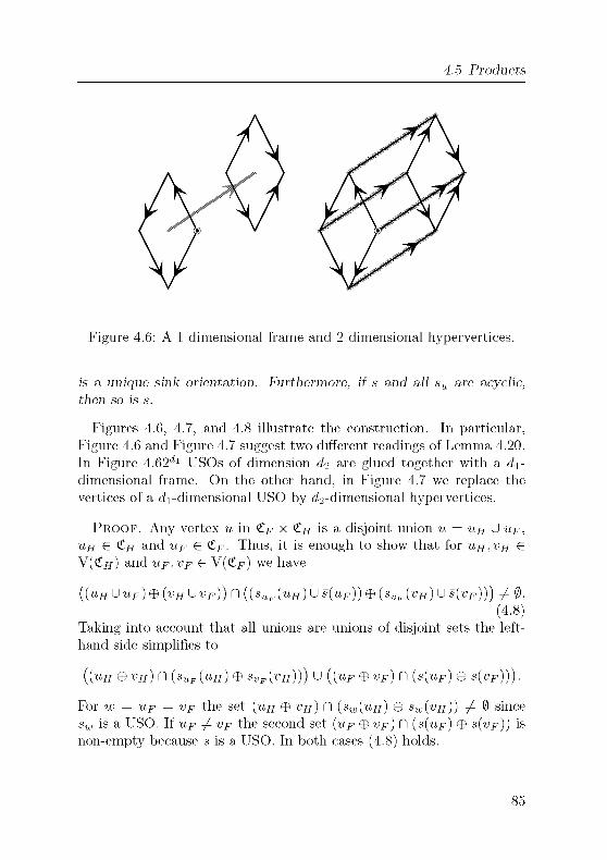
4.5 Products
Figure 4.6: A 1-dimensional frame and 2-dimensional hypervertices.
is a unique sink orientation. Furthermore, if s and all s„ are acyclic,then so is s.
Figures 4.6, 4.7, and 4.8 illustrate the construction. In particular,
Figure 4.6 and Figure 4.7 suggest two different readings of Lemma 4.20.
In Figure 4.62dl USOs of dimension d2 are glued together with a d\-
dimensional frame. On the other hand, in Figure 4.7 we replace the
vertices of a di-dimensional USO by d2-dimensional hypervertices.
Proof. Any vertex u in £p x £# is a disjoint union u = uu U up,
uh G £jf and up G .p. Thus, it is enough to show that for w#,-y# G
V(£ff ) and up, vp G V(£p) we have
((uH U up) ® ivH U vp)) n (isUF iuH) U s(uF)) © isVF ivH) U s(vF)j) ± 0.
(4.8)Taking into account that all unions are unions of disjoint sets the left-
hand side simplifies to
(iuH ®vH)n (sUF [uH] © sVF ivH))) U(iup® vF) n isiup) ® sivp))).
For w = up = vp the set («#- © vh) fl (sw(uu) ® swivn)) ^ 0 since
sw is a USO. If up ^ vp the second set (up ® vp) n (s(up) ® s(vp)) is
non-empty because s is a USO. In both cases (4.8) holds.
85

4 Structure
Figure 4.7: A 2-dimensional frame and 1-dimensional hypervertices.
For the second part of the lemma observe that a path u\VJvi,..., UkUvk
in £p x £# w.r.t. s induces a walk vi,...,Vk in £p w.r.t. s. If the
vertices u\ \J v\,.. .,Uk U vj. formed a cycle, i.e. ujUtii = «& U Vk,
then the induced walk v\,.. .,vj. either would contain a cycle in s or
v\ = v2 = = Vk = v. Since s is acyclic, we must have the second
case. But then u\,...,Uk forms a cycle in £# w.r.t. sv. This is a
contradiction to sv being acyclic, i.e., s has to be acyclic. D
For dim£p = 1, Lemma 4.20 says that we can combine two arbitrary
(d—l)-dimensional USOs to a d-dimensional USO by placing them in two
disjoint facets and directing all edges in between in the same direction.
An example for this case can be seen in Figure 4.6.
The other extreme case dim £# = 1 shows that if a cube contains
two opposite facets with the same (d— l)-dimensional USO s, the edgesbetween these facets can be directed arbitrarily. Figure 4.7 illustrates
this case. By Lemma 4.13 we already know that such USOs are the
only ones in which all edges of one label are flippable. But in addition
Lemma 4.20 guarantees them to be acyclic if s was acyclic.
86
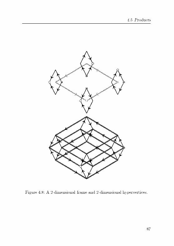
4.5 Products
Figure 4.8: A 2-dimensional frame and 2-dimensional hypervertices.
87
4 Structure
4.6 Examples
In the following we collect USOs that can be obtained by local changes
and/or a product construction. Even if the examples are rather simpleand straight-forward applications of Corollary 4.19 or Lemma 4.20 they
provide us with a good base. In fact, most concrete USOs used in the
literature belong to one of the following types.
4.6.1 Partial Unique Sink Orientations
Given a partial orientation on a cube £, under what circumstances can
this orientation be extended to a USO? We address this question in two
different ways. In the spirit of this chapter a USO is given by its outmap.
Hence, a partial USO would be a partial outmap. We will consider such
partial outmaps first. Afterwards we widen our view and consider partialorientations. In difference to partial outmaps such orientations do not
have to determine all edges in a vertex.
Let so : V(£) D D —> carr£ be a partial outmap. If so can be
extended to a USO s, this s must satisfy (4.2). In particular, for all
u, v G D we need
iu®v)n isoiu) ® soiv)) ^ 0.
It is not surprising that this condition is not sufficient for the existence
of s. Figure 4.9 shows an example of an orientation which is partially
good but cannot be extended.
The set D for which so from Figure 4.9 is defined consists of four
vertices. Hence, for |_D| > 4 the map so might not be extendible. We
will show that this is best possible. For |_D| = 2 there is always an
acyclic USO extending so and for |_D| =3 one can extend but might get
a cycle. (Since so already can have a cycle, see Figure 4.10).
Lemma 4.21 ([39, Corollary 4])For two vertices v\, V2 in a cube £ and sets Ai, A2 Ç carr £ with
(wi©w2)n(Ai©A2) ^0
there exists an acyclic unique sink orientation s with sirut) = At, i = 1,2.
88

4.6 Examples
Figure 4.9: A non-extendible partial USO. None of the given vertices
(marked with a black dot) contradict (4.2). But the gray
edges cannot be oriented without creating a 4-cycle.
Figure 4.10: A partial map with cycles. This map can be extended to a
USO by placing the global sink to the vertex o.
89

4 Structure
Proof. Choose A G (vi©v2)n(Ai©A2). Without restriction we can
assume A G Ai. Let t be the A-facet containing vt. On t let st be the
uniform orientation towards vt © (Aj \ {A}). According to Lemma 4.20
if we orient all A-edges towards £1 the resulting orientation s is a USO.
In s the vertex v\ has the outmap s{v\) = si(t>i) = v\ ®v\ © Ai = Ai
and V2 has s(v2) = S2(«2) © {A} = A2. As si and S2 are acyclic s is
acyclic.
Lemma 4.22
For three vertices vi,v2,vs in a cube £ and sets Ai, A2, A3 Ç carr £ with
(vt ® vj) C\ (At ® Aj) + %,
for i,j = 1,2,3, 1 ^ j there exists a unique sink orientation s with
s(wj) = Aj, 1 = 1,2,3.
Proof. Choose A G («i © «3) n (Ai © A3). Without loss of generality
v\ and v2 are in the lower A-facet £1 and V3, is in the upper A-facet £2. Bythe previous lemma we find a USO si on £1 with si(-yi) = Ai \ {A} and
si(w2) = A2\{A}. On £2 there is a USO s2 with s2(v2©{A}) = A2\{A}and S2ivs) = A2\ {A}. By Lemma 4.20 one can furthermore orient all
A-edges according to the A-edge in v\ and get a USO s'.
By construction s'(-yi) = Ai and s'(vs) = A3. Furthermore, for V2
only the A-edge might be oriented in the wrong direction. But this edgeis flippable, since s'(v2) © {A} = s'(v2 © {A}). After possibly flippingthis edge we found the desired orientation.
We now consider general partial orientations. That is, we drop the
restriction that the orientation is given by a partial outmap. In partic¬
ular, we are interested in sets of edges, such that any partial orientation
on this set can be extended to a USO.
Definition 4.23
A set of edges X in a cube £ is called extendible if for any orientation
4> on X there is a unique sink orientation extending </>.Let x(d) be the maximal cardinality of an extendible edge set in a
d-dimensional cube.
90

4 6 Examples
For instance, in dimension 2 any edge set of size 3 is extendible Such
set X consists of two edges of the same label, say label 2, and one edgeof different label, say label 1 No matter how the two edges of label 2
are oriented, if we choose for the 1-edge not in X the same orientation
as for the 1-edge in X, the resulting orientation is USO Since not every
orientation of £2 is USO, the set of all edges is not extendible Hence,
x(2) = 3
Lemma 4.24
x(d) > 2d - 1
Proof The claim is trivially true for dimension 1 Now assume Xd
is an extendible edge set in £d with 2d — 1 edges In £d+1 consider
Xd+i =XdU {{u © {d}, v © {d}} | {u, v} G Xd } U {{0, {d}}}
The set Xd+i consists of a copy of Xd in the lower d-facet, a copy of Xd
in the upper d-facet, and one d-edge
Any orientation of Xd+i can be extended to a USO with the helpof Lemma 4 20 Since Xd is extendible we find USOs si and S2 on
the lower and upper d-facet extending the two copies of Xd Now we
connect si and S2 by combing all d-edges according to the orientation
of {0, {d}} D
The bound is tight in dimension 3 It is also tight for d > 3 if we onlyallow edge sets for which (V(£),X) is connected
Lemma 4.25
Let X be an extendible edge set m £d', such that (V(£), X) is connected
Then \X\ < 2d - 1
Proof Let X be a set of at least 2d edges for which (V(£),X) is
connected We will show that such X is not extendible A spanning tree
of (V(£), X) has 2d — 1 edges If we add an additional edge from X to a
spanning tree, the resulting subgraph X' contains exactly one cycle C
On C place a cyclic orientation Edges not in C orient towards C The
resulting orientation </> cannot be extended to a USO For instance, see
Figure 4 11
91

4 Structure
Figure 4 11 An edge set with 2d edges The cycle is depicted by bold
lines The orientation drawn in the picture is not ex¬
tendible, since every vertex has an outgoing edge
If a vertex v G V(£) is in C it has an outgoing edge in C If v is not
in C, choose some u in C Since X' is connected, there is a path from v
to u We are only interested in the first edge of such a path This edgeis directed towards C, hence it is outgoing from v In particular, every
vertex in V(£) has at least one outgoing edge according to tp Hence,no extension of </> has a sink D
We will use Lemma 4 25 as the mam ingredient to prove that x(3) = 7
Nevertheless, for dimension 3 an exhaustive case distinction over all pos¬
sible X can still be done, either by computer or by a smart way of enu¬
merating the possible X For dimension 4 the number of configurationsis already too high
Lemma 4.26
x(3) = 7
Proof Let X be a set of 8 edges and assume that X is extendible
Since x(2) = 3, every facet has at most 3 edges Let x^ ' be the number
of edges in X and the upper A-facet Correspondingly, x^ 'is the number
of edges in X and the lower A-facet Double-counting yields
J2x^+xf = 2\X\ = m
X=l
92

4 6 Examples
This can only be achieved if four of the six facets have 3 edges In
particular, for some A both A-facets each have 3 edges in X Thus, the
vertices of the upper A-facet are in the same connected component of
(V(£), X), as well as the vertices of the lower A-facet Furthermore, two
A-edges are in X and connect the vertices in the two A-facets But then
(V(£), X) is connected in contradiction to Lemma 4 25
The arguments in the proof fail for dimension 4 The double counting
from above yields
E41)+40) = 32,
A=l
which can be achieved by xx = x°x = 4
4.6.2 Combed and Decomposable Orientations
Definition 4.27
A unique sink orientation s on a cube £ is A-combed if all A-edges are
directed the same way, l e
Vw,'yGV(£) A G s(u) ® s(v) <^=> A G u ® v
An orientation is combed if it is A-combed for some A G [d]
By flipping all A-edges pointing upwards (downwards) we can comb
any label A m a USO downwards (upwards) On the other hand, a A-
combed USO is product of its two A-facets with a 1-dimensional frame
It can be decomposed into two USOs of one dimension lower
Definition 4.28
A unique sink orientation is decomposable if every subcube is combed
See Figure 4 12 for a decomposable USO and Figure 4 13 for a combed
but not decomposable USO
4.6.3 Klee-Minty Cubes
The most famous representative of the class of decomposable cubes is
the so-called Klee-Mmty cube Every one-dimensional USO is a Klee-
Minty cube A d-dimensional cube is a Klee-Mmty cube if it is combed
93
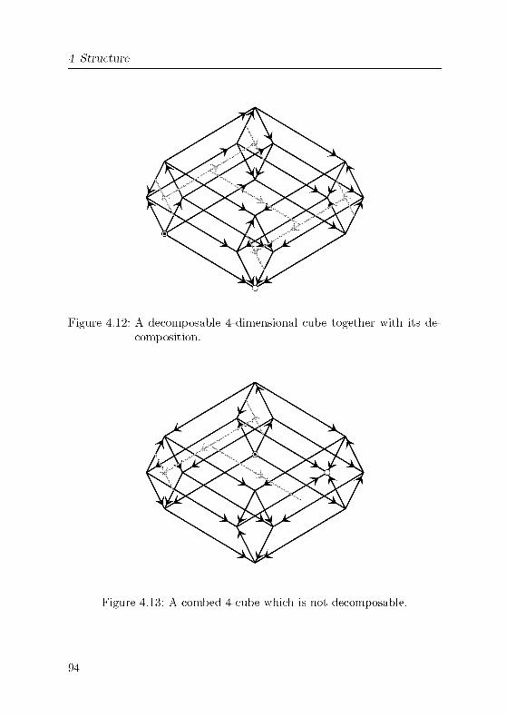
4 Structure
Figure 4.12: A decomposable 4-dimensional cube together with its de¬
composition.
Figure 4.13: A combed 4-cube which is not decomposable.
94
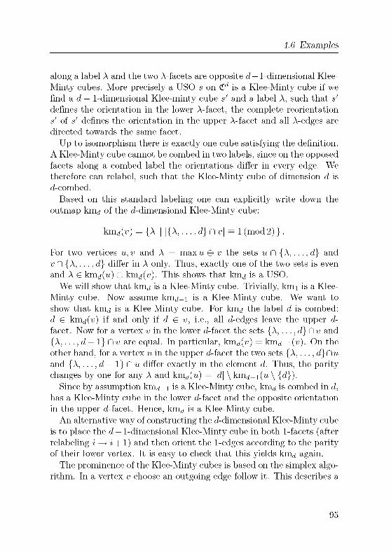
4 6 Examples
along a label A and the two A-facets are opposite d— 1-dimensional Klee-
Minty cubes. More precisely a USO s on £d is a Klee-Minty cube if we
find ad— 1-dimensional Klee-minty cube s' and a label A, such that s'
defines the orientation in the lower A-facet, the complete reorientation
s' of s' defines the orientation in the upper A-facet and all A-edges are
directed towards the same facet.
Up to isomorphism there is exactly one cube satisfying the definition.
A Klee-Minty cube cannot be combed in two labels, since on the opposedfacets along a combed label the orientations differ in every edge. We
therefore can relabel, such that the Klee-Minty cube of dimension d is
d-combed.
Based on this standard labeling one can explicitly write down the
outmap knid of the d-dimensional Klee-Minty cube:
kmd(w) = {A | \{A,...,d}Dv\ = l(mod2)}.
For two vertices u, v and A = max« © v the sets u n {A,..., d} and
v n {A,..., d} differ in A only. Thus, exactly one of the two sets is even
and A G ]smd(u) © \amd(v). This shows that km^ is a USO.
We will show that km^ is a Klee-Minty cube. Trivially, knii is a Klee-
Minty cube. Now assume km^-i is a Klee-Minty cube. We want to
show that knid is a Klee-Minty cube. For km^ the label d is combed:
d G km,j(w) if and only if d G v, i.e., all d-edges leave the upper d-
facet. Now for a vertex v in the lower d-facet the sets {A,... ,d}P\v and
{A,..., d — 1} n v are equal. In particular, km^-y) = km^i^). On the
other hand, for a vertex u in the upper d-facet the two sets {A,..., d}P\uand {A,..., d — 1} n u differ exactly in the element d. Thus, the parity
changes by one for any A and ~kmd(u) = [d] \ km,j_i(ti \ {d}).Since by assumption km^-i is a Klee-Minty cube, km^ is combed in d,
has a Klee-Minty cube in the lower d-facet and the opposite orientation
in the upper d-facet. Hence, km^ is a Klee-Minty cube.
An alternative way of constructing the d-dimensional Klee-Minty cube
is to place the d— 1-dimensional Klee-Minty cube in both 1-facets (afterrelabeling i —> i + l) and then orient the 1-edges according to the parityof their lower vertex. It is easy to check that this yields km^ again.
The prominence of the Klee-Minty cubes is based on the simplex algo¬rithm. In a vertex v choose an outgoing edge follow it. This describes a
95
4 Structure
simplex algorithm as soon as we give a pivot rule, i.e., a decision rule for
which outgoing edge to choose. Such simplex algorithms are normallystudied in the set-up of linear programming. Although they are fast
in practice, for nearly all deterministic pivot rules examples are known,on which the rule needs exponential many queries to find the optimum.
(See [3] for a survey.)We will discuss only a combinatorial simplex rule. Let SIMPLEX be the
simplex algorithm which chooses the edge with minimal label. Formally,Simplex in a vertex v will proceed with v © {min s(-y)}.
Proposition 4.29
The Simplex algorithm needs 2d queries to End the sink of the Klee-
Minty cube kind if it starts in its source.
Proof. The statement is trivially true for dimension 1.
The crucial observation is that the source of the lower d-facet is di¬
rectly below the sink of the upper d-facet. The global source is the
source in the upper d-facet. By induction SIMPLEX needs 2d_1 queriesuntil it queries the sink in the upper d-facet. Only then it will choose
a d-edge and proceed to the source of the lower d-facet. Again it needs
2d_1 queries to finally reach the global sink. Overall this adds up to 2d
queries.
4.6.4 Matching Flip Orientations
In the uniform orientation on a cube £ every subcube £' is a hypervertexand by Corollary 4.19 can be replaced by an arbitrary USO s. If after¬
wards one chooses a subcube £" disjoint from £' £" is a hypervertex
again and can be replaced. In general, this yields the following:
Lemma 4.30
Let s be the uniform orientation on £ towards a G V(£). For a family of
pairwise disjoint subcubes (£î)î=ij ^ of<t and unique sink orientations
st on £j, i = 1,..., k the orientation one obtains by replacing s on t
with Sj is a unique sink orientation.
Proof. As already mentioned by Corollary 4.19 we only have to show
that every £4 is a hypervertex. But as the £4 are mutually disjoint the
96

4.6 Examples
edges incident to a t are determined by s. As s is combed in all labels
£j is a hypervertex. D
A family of disjoint cubes of dimension 1, i.e., a set of disjoint edges is
a matching on £. In particular, every matching on £ gives a USO on £ by
flipping the matching edges in the uniform orientation. Furthermore, all
these orientations are mutually different. Such an orientation is called
matching flip orientation for obvious reasons. As there are dF1^2 ) perfect
matchings on a d-dimensional cube this shows:
Proposition 4.31 ([27])The number of unique sink orientations in dimension d is bounded from
below by dn{-2d\
97

4 Structure
Figure 4.14: The upper orientation is uniform. In the lower orientation
the gray subcubes are flipped.
98

4.7 Remarks
4.7 Remarks
The lower bound in Proposition 4.31 is sharp in the sense that the
number of USOs in dimension d is 2e(2 logd) (cf. page 16 and [27]).Thus, the simple proof of Proposition 4.31 is rather surprising. We will
see in the next chapter that matching flip orientations are very special.
In connection with isomorphisms the flippable edges of a USO play an
important role. Obviously, one has to check all flippable edges in order
to know if two USOs are isomorphic. In particular, whether a USO
is uniform cannot be checked without knowing all edges. From this
point of view the number of flippable edges is an interesting invariant
for checking isomorphy. Nevertheless, in high dimension nearly no two
USOs are isomorphic. The size of an isomorphism class is at most d!2d
whereas the overall number of USOs 2e(2 losd).
The question arises if there are USOs without flippable edges. The
answer to this question is closely related to a conjecture by Keller [22] :
A tiling of lRd by unit cubes is a collection of (geometric) unit cubes,such that each point x in Md is in one of these cubes and if x is in
more than one cube it is on the boundary of all cubes containing x.
Keller conjectured that in any such tiling we find two cubes, such that
their intersection is a facet of both of them. Szabo [41] showed that
Keller's conjecture can be decided on a much smaller class of tilings.The class introduced by Szabo is in one-to-one correspondence to d-
dimensional USOs and a tiling falsifies Keller's conjecture if and onlyif the corresponding USO has no flippable edge. For d < 6 Keller's
conjecture is true [36], but it gets false starting in dimension 8. (For a
counterexample in dimension 8 see [26], for dimensions 10 and 12 see
[25].) In particular, each USO of dimension less or equal 6 has a flippable
edge, whereas starting in dimension 8 there are USOs with no flippable
edge. The question remains open for dimension 7.
A flippable edge in a hypervertex is globally flippable. In particular,neither Corollary 4.19 nor Lemma 4.20 can construct a USO without
flippable edges from USOs with flippable edges. Thus, we cannot con¬
struct all d-dimensional USOs from lower-dimensional USOs using these
two construction schemes only.
The phase-concept is general enough to generate all USOs. Unfor-
99

4 Structure
tunately, it is too general to be used for concrete constructions. In
the following we will study algorithms for finding the sink. To achieve
lower bounds one often needs to extend a partial outmap to a USO. As
new vertices can produce new phase-dependencies such constructions
are hard to obtain using phases. In contrast local changes and productsturn out to be very useful for this purpose.
The Markov chain was first suggested by Valtr and Matousek [30].Unfortunately, its mixing rate is unknown. Still, it is the only known
method to produce a random USO with approximate uniform distribu¬
tion.
100

5 Algorithms
Sink him1
(Stubb)
101

5 Algorithms
5.1 Complexity Model
The mam interest in USOs is to solve Sink or SinkOrFalsify By
accessing the outmap the goal is to find the sink (1 e, query it) or to
give a certificate that the underlying orientation is not a USO The
characterization of unique sink outmaps (4 2) suggests certificates of
the form u,v with (u(&v) n (s(w)© s(v)) = 0 Nevertheless we still allow
for (much) longer certificates Consider an algorithm A for which it is
known that A needs at most t^(d) queries on a d-dimensional USO to
find the sink Then, for an outmap s, a sequence of queries longer than
tyl(d) is a certificate for s not being USO
Since in the complexity model for USOs we only count the number
of vertex evaluations, the problem does not directly relate to classical
complexity theory As seen in Chapter 3, we use USOs to solve other
problems via a well-behaved outmap In the following we reformulate
this connection in the setting of formal languages
Definition 5.1
For a language L G S* x S* over the alphabet £, the problem F(L) is
to End for any x G S* a y G S* such that (x, y) G L, or to decide that
no such y exists
The class of languages for which (x, y) G L can be decided m polyno¬mial time is called FNP The subclass of L G FNP for which FiL) can
be solved m polynomial time is called FP
The names FNP and FP are not chosen arbitrarily In fact, every
problem in NP has a variant in FNP For instance, Sat is equivalent to
{(x,y) | y satisfying assignment for formula x}
On the other hand, for F G FNP the language
TTiL = {x \3y (x,y) G L}
is in NP Thus, P = NP iff FP = FNP The notions of polynomial re-
ducibihty, completeness and hardness carry over to the functional vari¬
ants For a more detailed description, see [34, Chapter 10]In the problems studied in Chapter 3 we always had a parameter
which fixes the dimension for the corresponding USO In the setting of
102

5 1 Complexity Model
general languages it is more convenient to describe USOs in a way which
does not depend on the dimension
For the rest of the chapter, we assume without loss of generality X =
{0,1, *} In particular, we can describe cubes and subcubes as words in
X* Let
2<°° = {t>CN \v finite}
As before, we embed 2<0° into {0,1}* except now we do not fix the
dimension More formally, a set u G 2<0° is represented by the word w
of length max u with w\ = l -<=> A G m In particular, w ends with 1
A map s 2<0° —> 2<0° is a unique sink outmap iff for all u, v G 2<0°
condition (4 2) holds We say that such an outmap s has dimension
d if it is uniform outside 2^1, l e, s(v) = v for all v G 2<0° \ 2^1 In
particular, for a d-dimensional USO the cube £d is a hypersink of s in
2<oo This enhanced definition captures the original definition of USOs
By Corollary 4 19 we can embed any USO into the uniform orientation
on 2<°°
Definition 5.2
For a functional language LÇE* x X*, a unique sink oracle is a tuple
(<S, T) of functions
S X* _> (2<0° - 2<0°)T X* x 2<°° - X*
(called oracle S and interpreter T), such that for any x G tt^L, the map
Six) is a unique sink orientation, and for the sink o of this orientation,the interpretation y = T(x, o) satisßes ix, y) G L
A unique smk oracle is called polynomial if S(x)(-y) and T(x,v) can
be calculated m polynomial time m |x| and \v\, and the dimension of
Six) is polynomial m |x|
For instance, let L be the language, such that the first argumentencodes a feasible, bounded linear program LP(A, b, c), and the second
argument encodes a solution to LP(A, b, c) Then Definition 3 22 defines
an oracle S by Theorem 3 23 Furthermore, Proposition 3 25 yields an
interpreter T In particular, (<S, T) is a polynomial unique sink oracle
for linear programming
103

5 Algorithms
Oracle and interpreter are allowed to do anything on x ^ i^\L In
most cases, oracles are only meaningful on i^\L It might even be that
an algorithm for S or T does not terminate outside n\L
Assume for a moment that there is an algorithm for SinkOrFalsify
which needs polynomial time to find the sink Furthermore, assume
that there is a polynomial unique sink oracle for FSat Given some
x G 7TiFSat, by assumption, the sink o of the corresponding USO can
be found in polynomial time The interpretation y of o solves FSat
x Hence, such an oracle for FSat implies that SinkOrFalsify is not
polynomial provided P ^ NP
Theorem 5.3
Given an ~NP-complete problem L and its functional variant FL If
there exists a polynomial unique sink oracle for FL, then NP = coNP
Proof We will construct a polynomial time non-deterministic algo¬rithm which decides x ^ L This proves L G coNP As a consequence
NP = coNP
Let (<S, T) be the polynomial oracle for FL Consider the language
Ls = {(x,o) |<S(x)(o) = 0}U
{(x,m#w) | (u ® v) n (<S(x)(w) © S{x){v)) = 0}
With the conventions above, Ls is a language over X Furthermore, for
any x G X* the outmap <S(x) is either a USO (and thus we find x, o
with Six)io) = 0) or has two vertices failing (4 2) Thus, the projection
7Ti Ls equals X* In other words, Ls is total
The relation (x, y) G Ls can be checked in polynomial time The
dimension of S is polynomially bounded in |x|, say by p(|x|) After
scanning the first 2p(|x|) + 1 symbols of y, we can distinguish three
cases
(î) y is too long,
(u) y is of the form y = o, o G 2^x^\ or
(m) y is of the form y = ufj=v, u, v G 2^x^
104

5 2 A Lower Bound on Deterministic Algorithms
In the first case, (x, y) cannot be in Ls In the second case, we have
to check if Six)io) is empty And in the third case, we have to check
S(x)(u) © S(x)(v) = 0 Both can be done in polynomial time
Let x ^ L Consider the following algorithm For y G X*, first
check if ff appears more than once in y If so, y is rejected If ff
appears exactly once in y, say y = uffv, we can check in polynomialtime whether S(x)(u) © S(x)(v) = 0 If not, reject y, otherwise y is
a certificate for <S(x) not being a USO Thus, y certifies x ^ L If
# «Ë y and S(x)(y) ^ 0, reject y Otherwise, calculate y = T(x,y) If
(x, y) G FL then x G L, otherwise x ^ L All steps can be done in
polynomial time by assumption
Thus, the procedure just described decides in polynomial time if y is
a certificate for x ^ L This establishes L G coNP D
5.2 A Lower Bound on Deterministic Algorithms
The setup for this section is the following We are given an arbitrarydeterministic algorithm A for Sink and want to construct a USO on
which A needs "many" queries Rather than exploiting structural as¬
pects of such algorithms we do this in a game theoretic fashion We playa game against A In every move the algorithm queries a vertex and we
reveal the orientation in this vertex We have to answer according to
the outmap of a USO s This outmap will be constructed in an on-line
fashion depending on the queries of the algorithm At the end of the
game we have a concrete (acyclic) USO s for which A needs nearly a
quadratic number of queries
Given a deterministic algorithm A for finding the sink, we construct
an acyclic unique sink orientation of dimension d for which the algorithmneeds an almost-quadratic number of queries For the first d — [log2 d]inquiries, we maintain a partial outmap s W —> carr £d on the set
W G V(£d) of queried vertices, containing the answers we gave so far
We also maintain a set A of labels and an acyclic unique sink outmap
s on £A This smaller dimensional outmap s is our "building block"
which enables us to extend our answers to a global USO at any time
Before the first inquiry, we set A = W = 0 After each inquiry we
answer by revealing the value of the outmap s at the requested vertex
105

5 Algorithms
Then we update A and s, such that the following conditions hold.
(a) |A| < \W\,
(b) w' n A ^ w" n A for every w' ^ w" eW and
(c) s(w) = s(w n A) U [d] \ A for every w eW.
Informally, condition (6) means that the projections of the queriedvertices to £A are all distinct. This we shall achieve by occasionally
adding a label to A if the condition would be violated. Condition (c)exhibits two properties of our answers to the inquiries of the algorithm.
First, that our answers are consistent with s on A-edges, and second,that all ([d] \ A)-edges, i.e., the edges leaving the cube spanned by w
and A are outgoing.
Suppose now that the algorithm requests the evaluation of the next
vertex u. We can assume that u ^ W. Depending on whether there is
a w e W with wnA = wnAwe have to distinguish two cases.
Case 1. For every w G W, we have w C\ A y^ uC\ A.
Then we answer s(w) = s(w n A) U [d] \ A and leave A and s un¬
changed, (a) — (c) all hold trivially by the definition of the updates and
the assumption of Case 1.
Case 2. There is a v G W, such that u n A = v n A.
By condition (6), there is exactly one such v G W. The assumptionof Case 2 and u ^ v imply that we can fix a label A ^ A such that
A G u®v.
We answer s(u) = s(v) \ {A}. As A ^ A, the label A is in s(v).Now we have to update A and s. We get our new A by adding A.
To define the new orientation s, we take two copies of the old s on the
two facets determined by A. Then, by Lemma 4.20, we can define the
orientation of the edges going across arbitrarily, so we make them such
that the condition (c) is satisfied. More formally, let
{s(»nA)
if z = uC\ (AU {A})s(wnA)u{A} ifz = wn(Au{A})
for some w G W, w =£ u
s(z) U (z n {A}) otherwise.
106
5 2 A Lower Bound on Deterministic Algorithms
Next, we have to check conditions ia)~ic) for our new W, A and s
Condition (a) still holds, because we added one element to each of W
and A Since A just got larger, we only need to check condition (6) for
the pairs of vertices containing u By the uniqueness of v, it is actually
enough to check (6) for the pair u, v Since A was chosen from u® v and
now is included m A, «flA^snA Condition (c) is straightforwardfrom the definitions
We proceed until \W\ = d — [log2 d], and then change the strategy
By condition (a), |A| < d— [log2 d] We choose an arbitrary superset A'
of A such that |A'| = d— [log2 d] The set of labels [d]\A' determines at
least 2d~'A I > d disjoint subcubes generated by A' As IV^I < d, we can
select one of them, say £o, which does not contain any point evaluated
so far
Our plan is to apply a local change with £o and an orientation s,
which is consistent with the outmaps of the vertices evaluated so far
Corollary 4 19 then will enable us to reveal s on V(£d) \ V(£o) to the
algorithm and still be able to start a completely "new game" on £o, a
cube of relatively large dimension To construct s satisfying the condi¬
tions of Lemma 4 18, we use the product construction of Lemma 4 20
twice
First we define an orientation s of £A using the product construction
for s on the frame £A and outmaps sv on the hypervertices along £A \A
with the property that for every w G W, the map swri^ has its source at
w n (A' \ A) This last requirement can be satisfied because of condition
(6) For v se W the map sv can be arbitrary
Thus, the resulting outmap s is consistent with the evaluated vertices
m the sense that s(w) n A' = s(w n A') for each w G W
Next, we use again the product construction with s on the frame £A,
so we have to construct USOs sv of £ldl\A for every v G V(£A ) In
doing so, we only take care that the sinks of all these orientations are
m £o, and if v = w n A' for some w G W, then w \ A' is the source of
sv (By condition (6), there can be at most one such vertex w for each
v ) The appropriate sv exists according to Lemma 4 21 Now applythe product construction with frame s and the hypervertices sv This
provides us with an orientation s which agrees with our answers given
for the evaluated vertices Furthermore, £o is a hypersink w r t s
We can reveal s on V(£d) \ V(£q) and still be able to place any orien-
107

5 Algorithms
tation on £o, a hypersink of dimension d — [log2 d] Therefore, we just
proved
tacycid) >d- [fog2 d] + tacydd - [log2 d] )
Theorem 5.4 ([39, Theorem 9])Any deterministic algorithm needs Q(j^-^) many vertex evaluations to
ßnd the sink of an acyclic unique sink orientation on a d-dimensional
cube
Proof We prove by induction for d > 2
d2 d
2[log2dl 2
Since tacyci2) > 1 = § — § and tacyci-3) > 1 > | — |, the inequalityholds for d = 2, 3
Now let d > 4 By induction for 2 < k < d we have tacycik) >
2\iog2k-]~ I Smce d ~ rioS2 d] > 2 we get
tacycid) > d- [fog2 d] + tacycid - [log2 d] )
> d - [log2 d\ +
,(d-[log2dl)2 1
2[log2(d-[log2dl)l 2
i -2rios2 ^i +
d2 - 2d[log2 d] + [log2 d]
(d-[log2dl)
>2d_2^l0g2^
2[log2dl
d
2[log2dl 2'
and the inequality also holds for d D
5.3 Small Dimensions
For dimension 0, t(0) = 1, since there is no edge This is a good oppor¬
tunity to point out once more that we require the sink to be queried,
108

5 3 Small Dimensions
even if (as in this case) we know where it is For dimension 1, obviously
t(l) = 2
After querying the vertices of even cardinality in a USO s, the position
of the sink is known In fact, then we know the whole orientation
In particular, this shows that t(2) < 2 + 1 = 3 and t(3) < 4 + 1 =
5 In the following, we not only show that this simple algorithm is
best possible In both dimensions, this bound is sharp even on the
set of acyclic orientations Furthermore, we can forbid a vertex in the
beginning
Proposition 5.5 ([39, Proposition 10])Every deterministic algorithm needs three queries to ßnd the sink of a
two-dimensional unique sink orientation, even if there is a ßxed vertex
which is known not to be the sink In particular, t(2) = 3
Proof The strategy answers with the source for the first query of an
algorithm Now, all remaining three unquened vertices are still potentialsinks by Lemma 4 21 Even if one of them is known not to be the sink,there are two possibilities left Therefore, no deterministic algorithmcan evaluate the sink in two steps D
As in the general lower bound, the mam tool in the following is pro¬
vided by Lemma 4 18 We will construct a partial outmap with a hy¬
persink Since the sink has to be located in this hypersink, we can then
proceed recursively, using Lemma 4 18
Proposition 5.6 ([39, Proposition 11])Every deterministic algorithm needs ßve queries to ßnd the sink of a
three-dimensional acyclic unique sink orientation, even if there is a ßxed
vertex which is known not to be the sink In particular, t(3) = 5
Proof Let A be some algorithm for Sink and u be the vertex which
is known not to be the sink We construct an example s on £3 for which
A needs 5 steps at least
The first query v\ will be answered with the source, s{v\) = [3] If the
second query -y2 is not antipodal to v\, both vertices are in a common
facet, say A ^ v\ © -y2 In this case set s(v2) = {A} Combing all
A-edges towards the A-facet £q not containing v\ and -y2 makes £q a
109

5 Algorithms
2-dimensional hypersink. Any algorithm needs 3 more queries to find
the sink in £o, even if the non-sink u is in £].If the second query -y2 is antipodal to v\, choose some A G V2 ® u
if u ^ V2 or A = 1 otherwise. Without loss of generality, v\ = 000,
V2 = 111 and A = 1. For all four edges *10, 1*0, 10* and *01, there is
an acyclic USO having the edge as hypersink (cf. Figure 5.1). At most
one of the edges contains u (as u = -y2 or u G 0**) and at most two
edges are blocked by the third query. Therefore, after 3 queries there is
a 1-dimensional hypervertex for which any algorithm needs 2 additional
queries to find the sink. D
One can prove even stronger statements. For instance, it is true that
even the knowledge about two fixed points of distance either three or
one that neither is the sink would not help an algorithm to find the
sink: it would still need to evaluate 5 vertices. Curiously, if it is known
about two vertices of distance two that neither is the sink, an algorithm
finding the sink in 4 steps exists.
Proposition 5.7 ([39, Proposition 12])Every deterministic algorithm needs at least seven steps to ßnd the sink
of a four-dimensional acyclic unique sink orientation.
Proof. The first query vi of an algorithm A will be answered bythe source, s(-yi) = [4]. For the second query v2, choose a A G vi © -y2
and answer s(v2) = [4] \ {A}. Without loss of generality A = 1 and
Vl = 0000.
If v\ and V2 are not antipodal, we comb label 4. Thus, the facet
£' along label 4 not containing v\ and -y2 is a hypersink. Since any
algorithm needs 5 steps to find the sink in £' we need 7 steps altogether.For the rest of the proof assume v\ and -y2 are antipodal, i.e., v\ = 0000
and V2 = 1111. Our goal for the next two queries is to keep a 2-
dimensional hypersink unqueried. Since then we can force A into 3
more queries. In the following we fix two USOs si and s2. Our answers
up to the fourth query rely either on s i or on s2.
We now construct si. Let s be the bow on £00** with sink in 0010 and
source in 0011. Construct a USO so with frame s using Lemma 4.20.
The hypervertices are s«0o = «**oi = «**io = ©h and s«n is the bow
with source in 0011 and sink in 1011 (cf. Figure 5.2).
110

5.3 Small Dimensions
Figure 5.1: The orientations forcing 5 steps in dimension 3.
Ill

5 Algorithms
Figure 5.2: The construction of si.
In si the subcube 00** is a hypersource. We can replace this hyper-source with the bow having its sink in 0010 and source in 0000. The
resulting USO si is acyclic. See Figure 5.3 for a picture of si. For s2
flip the two edges 01*0 and 11*0 in si. In fact, both edges are flippable.
Hence, s2 is a USO. See Figure 5.4 for a picture of s2.
We only need some facts about si and s2. First of all, both orienta¬
tions agree on all vertices outside the faces **10 and *10*. Furthermore,for v\ and -y2 the outmap-values coincide with the answers we gave. And
finally, for si the face **10 is a hypersink, whereas for s2 the face *10*
is a hypersink.We are now ready to deal with the remaining queries of A. For the
third query v3 there are six cases with respect to v\ © v3. So far we onlyfixed label 1. All other labels can still be permuted without affecting
s(-yi) or s(v2). According to the six cases we now decide on the other
three labels.
(1) v1 ® v3 = {1}. Then v3 is the vetex 1000.
(2) vi ® v3 = {/j,}, p^l. Then set /x = 4, i.e., v3 = 0001.
(3) v\ © v3 = {1, /x}, /i^l. Then set /x = 4, i.e., v3 = 1001.
112
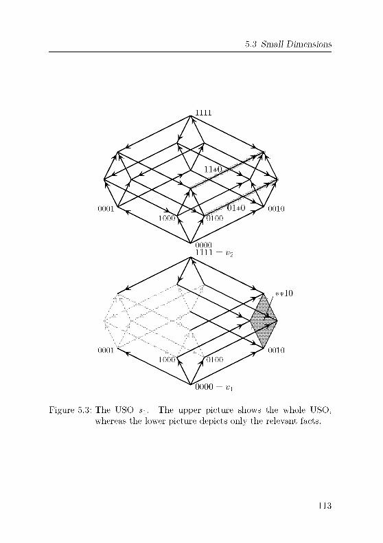
5.3 Small Dimensions
1111
0001 0010
**10
0001 0010
0000 = Vl
Figure 5.3: The USO si. The upper picture shows the whole USO,whereas the lower picture depicts only the relevant facts.
113

5 Algorithms
Figure 5.4: The USO s2. The upper picture shows the whole USO,whereas the lower picture depicts only the relevant facts.
114

5 3 Small Dimensions
1111 = V2
Figure 5.5: The possible positions of v3. The gray shaded area covers
the subcubes where we still want to change the orientation
according to the remaining queries.
(4) vi®v3 = {/x, i/}, /x, v ^ 1. Then set /x = 4 and v = 3, i.e., v3 = 0011.
(5) Vi ® v3 = [4] \ {/x}, p^l. Then set /x = 2, i.e., v3 = 1011.
(6) Vi ® v3 = {2, 3,4}. Then v3 is the vertex 0111.
See Figure 5.5 for the possible positions of v3. In no case the two 2-
faces *10* and **10 contain a queried point. Answer to v3 according to
siiv3) = s2(v3).If the fourth query V4 is not in **10 we fix s(v) = si(-y) outside **10.
Since **10 is hypersink in si, we can replace the orientation in this face
arbitrarily and force the algorithm into 3 more queries to find the sink
in **10. This makes 7 queries altogether.If on the other hand V4 is in **10, we fix s(v) = s2(v) outside *10*
and proceed as above. D
This proof provides us with a very small class of 4-dimensional USOs
on which every deterministic algorithm needs 7 queries at least. Fur¬
thermore, the constructed USOs are rather simple. One would therefore
115
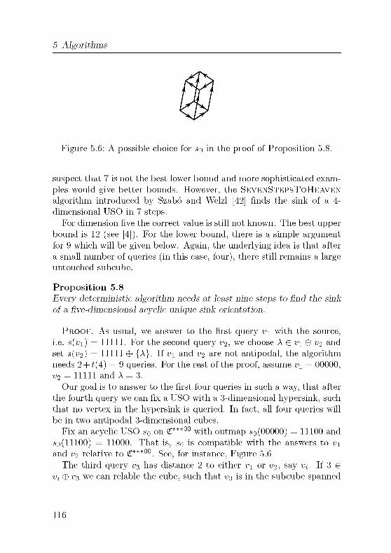
5 Algorithms
Figure 5.6: A possible choice for so in the proof of Proposition 5.8.
suspect that 7 is not the best lower bound and more sophisticated exam¬
ples would give better bounds. However, the SevenStepsToHeaven
algorithm introduced by Szabo and Welzl [42] finds the sink of a 4-
dimensional USO in 7 steps.
For dimension five the correct value is still not known. The best upper
bound is 12 (see [4]). For the lower bound, there is a simple argument
for 9 which will be given below. Again, the underlying idea is that after
a small number of queries (in this case, four), there still remains a largeuntouched subcube.
Proposition 5.8
Every deterministic algorithm needs at least nine steps to ßnd the sink
of a ßve-dimensional acyclic unique sink orientation.
Proof. As usual, we answer to the first query v\ with the source,
i.e. s(-yi) = 11111. For the second query v2, we choose A G v\ ® V2 and
set s(v2) = 11111 © {A}. If Vi and -y2 are not antipodal, the algorithmneeds 2 + t(4) = 9 queries. For the rest of the proof, assume v\ = 00000,
-y2 = 11111 and A = 3.
Our goal is to answer to the first four queries in such a way, that after
the fourth query we can fix a USO with a 3-dimensional hypersink, such
that no vertex in the hypersink is queried. In fact, all four queries will
be in two antipodal 3-dimensional cubes.
Fix an acyclic USO s0 on £***00 with outmap s0 (00000) = 11100 and
so (11100) = 11000. That is, so is compatible with the answers to v\
and V2 relative to £***00. See, for instance, Figure 5.6
The third query v3 has distance 2 to either v\ or v2, say vt. If 3 G
vt © v3 we can relable the cube, such that v3 is in the subcube spanned
116
5 3 Small Dimensions
by vt and the labels 2, 3. Otherwise, we can assume that v3 is in the
subcube spanned by vt and 1,2. See Figure 5.7.
We answer to v3 either s(vs) = soiv3 n {1, 2, 3}) U {4, 5} if i = 1 or
s(v3) = soiv3 n {1, 2, 3}) U {5} if i = 2.
If vt © v3 G {2, 3}, we can always achieve that V4 is in one of the
subcubes £***00 or £***n. See Figure 5.8.
For vt © v3 G {1,2} after relabeling the fourth query V4 is either in
one of the subcubes £**00* and £**n* or in one of the subcubes £***00
or £***". See Figure 5.9.
If all four queries Vi,... ,V4 are in £**00* and £**n*, we construct the
final answer s by using Lemma 4.20 with a 2-dimensional frame and 3-
dimensional hypervertices. For the frame orientation s on £00**0 choose
the bow with source in 00000 and sink in 00100. For the hypervertices£**00* and £**n* choose orientations compatible with the answers to v\,
v2, and v3. (Such USOs exist by Lemma 4.21.) Answer to V4 accordingto this construction. For the remaining hypervertices £**01* and £**10*
we can choose arbitrary acyclic USOs. In particular, we can force 5
more queries in £**01*. See Figure 5.10.
If on the other hand all four queries Vi,... ,V4 are in £***00 and £***n,we use Lemma 4.20, now with a 3-dimensional frame and 2-dimensional
hypervertices. The frame orientation is s = sq. For the hypervertices we
always choose the bow with source in ***00 and sink in ***01, exceptfor the hypervertex in 11100. There we choose the bow with source in
***11 and sink in ***01. See Figure 5.11. The resulting orientation
is compatible with the answers so far. Answer to V4 according to this
construction. Furthermore, £***01 is a hypersink. Thus, we can force
five more queries.
D
The idea of the four proofs above looks promising at first sight: After
the first few queries, there are still untouched large subcubes. Unfortu¬
nately, in general, for fixed k the number of vertices one has to query to
pierce every (d — A;)-dimensional subcube is only logarithmic in d (see[2]).
117

5 Algorithms
ooioo
°**00 \lil 00010
10000
00100
D0O10.
1**11
DQQÛ1
00001
10000**000
Figure 5.7: The possible positions of v3. The gray shaded area covers
the subcubes where v3 can be found.
118

5.3 Small Dimensions
ooioo
***00 xJJJlf O0O10
***11
ÜQQQ1
'10000
Figure 5.8: The possible positions of V4 provided vt © v3 Ç 01100. The
dark gray shaded area covers the subcubes where v3 can be
found, whereas V4 can be found in the light grey.
119

5 Algorithms
Figure 5.9: The possible positions of V4 provided v% ® v3 G 11000. The
dark gray shaded area covers the subcubes where v3 can be
found, whereas V4 can be found in the light grey.
120

5.3 Small Dimensions
**11*
h.s. **10*
ooioo
**01*
-00001
**00*
'loooo
Figure 5.10: The construction for vl7..., vA G £**uu* u**00* i i 0***11*
00100
00001
Figure 5.11: The construction for vl7..., vA G £***uu u***00 i i a1***!!
121

5 Algorithms
5.4 Fast Subclasses
A matching flip orientation s, as defined in Section 4.6.4, is given by a
vertex o and a matching M: s is obtained by flipping the edges in M
in the uniform orientation ©ô- In ©0 every vertex v fulfills the equation
®ôiv) ® v = o. In other words, if one knows that a USO s is uniform
then with two queries one finds the sink: First query an arbitrary vertex
Vi and then v2 = s(v\) @ v\.
If s is a matching flip orientation given by o and M, then s(v) © v
must no longer be o. But M has at most one edge adjacent to v and
therefore s(v) © v has at most distance one to o. Furthermore, the sink
o of s is either a neighbor of ô or ô itself: If o ^ o, there has to be an
edge adjacent to ô in M. But then o is the other vertex incident with
this edge.This observation allows us to find the sink with 5 queries. After
the first query we are already very close to the sink. Exploring the
structure near ô we need 4 more queries in the direct neighborhood of
ô independent of the dimension.
Proposition 5.9 ([39, Proposition 8])In a matching ßip orientation s, the sink can be found in at most 5 steps
(independent of the dimension of s). The value 5 here is best possible,
except in dimension < 2.
Proof. Let s be obtained by flipping the edges of a matching M in
©ô- After querying an arbitrary vertex v\, the vertex -y2 = s{v{) ® v\ is
a neighbor of o. Thus, -y2 has at most two outgoing edges.
Obviously, -y2 is our next query. If |s(-y2)| = 0, we have found the sink
in two steps.
For |s(-y2)| = 1, we ask v3 = -y2 © s(v2) next. If v2 was o, v3 has to be
the sink. Otherwise, v3 = ô and either v3 is the sink or V4 = v3 © s(vs).Therefore, after at most four queries, we found the sink.
For |s(-y2)| = 2 we know that -y2 is a neighbor of ô and so is v3 =
V2 ® s(v2). Either v3 is the sink or V4 = v3 © (s(vs) fl s(v2)) is the
original ô and we need one more query to find the sink. This makes five
queries altogether.On the other hand, after answering the first query v\ the source, its
antipodal vertex Vi, and all neighbors v G N(vi) of vi are potentially the
122
5 4 Fast Subclasses
sink. Until one of these vertices is evaluated we answer to all queries
according to ©Cl. (Since all edges of one label could be flipped, our
answers do not reveal any information on vi or N{v\).) To find the sink
among the vertices in N{v\)\J{vi}, four queries are needed. This proves
the optimality. D
In the above algorithm, the first step made the most improvement, as
Vi could have been anywhere and v2 = s(vi) ® v^ is close to the sink.
In general, v © s(v) will not improve with respect to the distance to the
sink. (For instance, if source and sink are neighbors and v is the source.)But if s is combed then v © s(v) will be in the facet which is a hypersink
according to the combed direction.
Proposition 5.10 ([39, Proposition 7])For a decomposable unique sink orientation of dimension d, one needs
at most d + 1 vertex evaluations to evaluate the sink Moreover, d + 1
is best possible
Proof. Let s be a decomposable orientation and o its sink.
The observation above suggests the following algorithm: Start by
evaluating an arbitrary vertex v\, then perform the following procedure.For any i, if s(wj) = 0 then stop: vt is the sink. Otherwise, set vl+i =
vt © s(-yj) and repeat.
We show by induction that for each i, both the sink o of the orientation
and vt are in a (d —« + l)-dimensional hypersink. This implies that vn+i
is the sink.
The claim is true for i = 1 as the whole cube is a hypersink (nooutgoing edges). Suppose now that it is true for i. Since the orientation
is decomposable, the hypersink £4 containing vt and o is combed in
some label A. Say £î+i is the facet of £4 with incoming A-edges. As £4
is a hypersink of dimension (d — i + 1) the facet £î+i is a hypersink of
dimension d — i.
Furthermore, since vt G £j, only edges in £4 can leave vt. lfvt ^ £j+i,then A G s(-yj), otherwise A «Ë s(-y4). In particular, vl+i = vt © s(wj) G
For optimality, suppose an algorithm first requests the vertex v\. We
(the oracle) return the source, s{v{) = [d]. Let -y2 be the second request
123
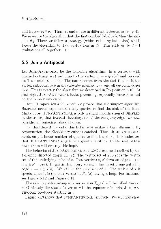
5 Algorithms
and let A G Vi®v2. Thus, -y2 and v\ are in different A-facets, say w2 G £2-We reveal to the algorithm that the first combed label is A, thus the sink
is in £2. There we follow a strategy (which exists by induction) which
forces the algorithm to do d evaluations in £2. This adds up to d + 1
evaluations all together. D
5.5 Jump Antipodal
Let JumpAntipodal be the following algorithm: In a vertex v with
queried outmap s(v) we jump to the vertex v' = v © s(v) and proceeduntil we reach the sink. The name comes from the fact that v' is the
vertex antipodal to v in the subcube spanned by v and all outgoing edgesin v. This is exactly the algorithm we described in Proposition 5.10. At
first sight JumpAntipodal looks promising, especially since it is fast
on the Klee-Minty cube.
Recall Proposition 4.29, where we proved that the simplex algorithmSimplex needs exponential many queries to find the sink of the Klee-
Minty cube. JumpAntipodal is only a slight modification of Simplex
in the sense, that instead choosing one of the outgoing edges we now
consider all outgoing edges at once.
For the Klee-Minty cube this little twist makes a big difference. By
construction, the Klee-Minty cube is combed. Thus, JumpAntipodal
needs only a linear number of queries to find the sink. This indicates,that JumpAntipodal might be a good algorithm. In the rest of this
chapter we will destroy this hope.
The behavior of JumpAntipodal on a USO s can be described by the
following directed graph Tapis): The vertex set of Tap(s) is the vertex
set of the underlying cube of s. Two vertices v, v' form an edge v —> v'
if v © v' = siv). In particular, every vertex v has exactly one outgoing
edge v —> v © s(v). We call v' the successor of v. The sink o of s is
special since it is the only vertex in Tap(s) having a loop. For instance,
see Figure 5.12 and Figure 5.13.
The unique path starting in a vertex v in Tap(s) will be called trace of
v. Obviously, the trace of a vertex v is the sequence of queries JumpAn¬
tipodal produces starting in v.
Figure 5.13 shows that JumpAntipodal can cycle. We will now show
124
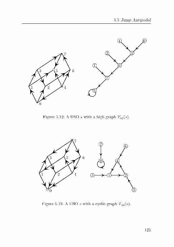
5 5 Jump Antipodal
Figure 5 12 A USO s with a high graph Tap(s)
(D
OX (4)
-*—CD—*—C2)
Figure 5 13 A USO s with a cyclic graph Tap(s)
125

5 Algorithms
that this can only happen in cyclic USOs The vertex v is a source in the
cube spanned by v and v © s(v) The following lemma provides us with
a path v ^* v ® s(v) Hence, the trace of JumpAntipodal induces a
trail in s and if JumpAntipodal cycles, the induced trail contains a
cycle of s
Lemma 5.11
Let s be a unique sink orientation on £ and v a vertex m £ Then there
is a path m the USO from the source of s to the sink of s via v
Proof We will prove the statement by induction on the dimension
d of £ For d = 1 the statement is trivially true Now assume, we known
that in any (d— 1)-dimensional USO there is a path from source to sink
via a given vertex v
For a d-dimensional USO s and a vertex v we will split the USO into
two facets and apply induction to the facets Let o be the sink of s and
w its source Choose A G o ® w Then o and w are in different A-facets
£i and £2, say o G £i and w G £2 Let w\ be the source of £1 and o2
the sink in £2
If v G £1, consider w[ = wi © {A} The vertex w[ is in £2 and byinduction we find a path w —>* w[ The A-edge {w[,wi} is directed
towards wi, since wi is not the global source Thus, we find a pathw —>* Wi But now by induction applied to £1 we find a path w^ —>*
v —>* o See the picture on the left in Figure 5 14
If v G £2 we repeat the arguments from above with the interim vertex
o2 = 02 ® {A}, that is, we find a path
* * / *
w —> V —> 02^02^ o
See the picture on the right in Figure 5 14 D
In the following, we only consider USOs for which JumpAntipodal
does not cycle For such USO s the graph Tap(s) is a tree, the so-called
bottom-antipodal tree This tree was first introduced by Kaibel [20] in
connection to randomized simplex algorithms In particular, Kaibel
raised the question, how high such a tree can be The height of a vertex
v in Tap (s) differs by one from the number of queries of JumpAntipodal
starting in this vertex Thus, if we can construct a family of examples
126

5 5 Jump Antipodal
Figure 5 14 How to find a path trough v The picture on the left side
shows the situation when v and o are separated from w bya label A The picture on the right side shows the reverse
situation, where v and w are separated from o
for which the maximal height grows exponentially JumpAntipodal has
complexity Q(2d) We will even show, that the average height (that is,
the arithmetic mean of the heights of all vertices) grows exponentially
Theorem 5.12
In every dimension d there is an acyclic USO, such that the height of
the corresponding bottom-antipodal tree is at least a/2 and the average
height isi^)d
Proof We will inductively construct acyclic USOs s^ on £d with
maximal height hid) = 2h(d—2)+2 and average height hid) > |/i(d—2)Fix some orientations s^2' and s^3' For instance, we can choose the
orientations of height h(2) and h(3), repectively That is, for s^ choose
a bow and for s^ choose the orientation in Figure 5 12
Now assume we have already constructed s(d~2) Without restriction
we assume that s(d~2) has its sink in 0 Let T = Tap(s(-d_2^) be its
bottom-antipodal graph, o its sink and vmax a vertex of maximal heightBased on s(d~2) we use Lemma 4 20 and Lemma 4 18 to construct s^
As an intermediate step we construct a d-dimensional s' by applyingLemma 4 20 with frame s(d~2) The hypervertices are one of the two
bows so and si with sink in 0 and source in {d— 1} and {d}, respectively
127

5 Algorithms
Vertices of s(d~2) with an even height in T are replaced by so and vertices
of odd height by si. Formally, for v G £d~2 with height congruent i
modulo 2 set sv = st and let s' be the product of all sv with frame
s(d-2) according to Lemma 4.20.
Since so and si have the sink at the same vertex, by construction the
subcube * • • • *00 is a hypersink of s'. In this hypersink replace s(d~2)
by s(d~2) o ©t,max. That is, we change s(d~2) in * • • • *00, such that the
sinks of the other three copies in * • • • *01, * • • • *10, and * • • • *11 are
above the vertex vmax in * • • • *00.
The resulting USO is s = s^d'. As bows and s^d^2' are acyclic, so is
s.
Color the vertices of £d according to their position in the {d — 1, d}-hypervertices: a vertex is blue if it is in the sink of a hypervertex, it
is green if in a hypervertex it is antipodal to the sink, and it is yellowif it is the source of a hypervertex. The remaining vertices are red. In
other words, the vertices in * • • • *00 are colored blue and the vertices
in *---*ll green. The remaining vertices are colored yellow if their
{d— 1, d}-edges are outgoing and red otherwise. We will refer to the set
of blue vertices by B, the set of green vertices by G, the set of yellowvertices by Y, and the set of red vertices by R.
For a vertex v define hpiv) as the height of v in the corresponding
copy of s(d~2\ Formally, for a non-blue vertex v the height hr{v) is the
height of v n [d — 2] in T. A blue v lives in a shifted copy of s(d~2\ thus
for such v the height hpiv) is the height of v P\ [d — 2] © vmax in T. In
the following we want to express the height h(v) in Tap(s^) in terms
of hr{v). The blue subcube is a hypersink. Thus, a blue vertex v has a
blue successor. In particular, h(v) = hr{v).Next we study the height of the vertices 0 • • • 000, 0 • • • 010, 0 • • • 001,
and 0 • • • 011. By assumption, on s^d~2\ the vertices 0 • • • 010, 0 • • • 001,and 0---011 are the sink in their corresponding copy of s(d~2\ We
exchanged the orientation in the subcube * • • • *00, such that the sink
and Dmax change position. Hence, 0 • • • 000 has height
h{0 • • • 000) = hT{0 • • • 000) = hid - 2).
By choice of so the vertex 0 • • • 010 has only the (d — l)-edge outgoing.
128

5.5 Jump Antipodal
Thus, its successor is 0 • • • 000 and
h{0 • • • 010) = 1 + h{0 • • • 000) = l + h{d-2).
Similarly, the vertex 0 • • • 001 has outgoing edges of label d — 1 and d
and its successor is 0 • • • 010. Therefore
h{0 • • • 001) = 1 + h{0 • • • 010) = 2 + h{d-2).
Finally, the vertex 0 • • • 011 has the d-edge outgoing and
h{0 • • • 011) = 1 + h{0 • • • 010) = 2 + h{d-2).
The remaining vertices are classified by their color. In general, red
vertices have blue parents. Let v be a red vertex. It's outmap s(v)consists of two components, s(v) = s(d~2\v(~) [d— 2])©Sj(-yn{d — 1, d}).Since v is red, Sj(-y n {d — 1, d}) has one outgoing edge which pointstowards the sink of this hypervertex. Hence, v © s(v) relative to the
corresponding hypervertex will be in the sink, i.e., blue.
A yellow vertex v y^ 0 -010 has a yellow successor v' with height
hriv) = 1 + hpiv'). Again, we consider the two components s(v) =
s(d-2)(v n [d - 2]) © stiv n {d - 1, d}). Relative to the frame s^2) the
vertex v P\ [d — 2] has a successor v[. Relative to the hypervertex st the
vertex vP\{d—l,d} has its antipodal vertex v'2 as successor. Hence, the
successor of v is v' = v[ © v2. In particular, hpiv) = 1 + hr{v'). Since
v[ has a different parity than vP\{d—l, d}, we now are in a hypervertexof different type s}. In s} the source is antipodal to the source of st.
Hence, v' © v" is yellow.A green vertex v ^ 0 • • 011 has a yellow successor. We can copy
the argument from above. Again, v" = Sj(-y) is antipodal to the source
relative to st .
Now consider the green vertex u = vmax U {d — 1, d}, i.e., the green
vertex with hr{u) = hid — 2). The trace of u will consist of yellow
vertices, until we hit the yellow sink 0 • • • 010. Hence, we get
hid)>hiu) = hTiu) + hi<d {)!{))
= h{d-2) + l + h{d-2) = 2h{d-2) + l.
This proves h(d) > \/2 .
129

5 Algorithms
For the average height hid) we forget about the red vertices (as we
don't know their height) and get
~h(d) = Yd^h{v)v
\vEB vEY vEG J
= ^(Em«) + £(m<>) +! + >*(<*-2» +\vEB vEY
+ Y/(,hTiv) + 2 + hid-2))\vEG )
4•
^2 E M«) +4
•
^2 E M*HEß CEF
1 1
4 2d-2 ^J w
2dueG
> ^hid-2)+l-hid-2)> \h{d-2).
This proves that h{d) > i^)d. D
U E M«) + i(2d_2 +2"_1 +^^ "2))
130

5 6 Remarks
5.6 Remarks
In terms of classical complexity theory, Theorem 5 3 relies on the fact
that a polynomial unique sink oracle induces a total relation The class
of all total relations in FNP is called TFNP It is known that a FNP-
complete problem in TFNP would imply NP = coNP (see [31, Theo¬
rem 2 1]) In this sense, the mam part of Theorem 5 3 is to show that
a polynomial unique sink oracle defines a language in TFNP
The best known algorithms for solving Sink can be found in [42] The
algorithm FiBONACClSEESAW needs 0(1 61d) queries to find the sink in
a d-dimensional USO The best randomized algorithm needs 0(1 44d)expected queries If we restrict our attention to acyclic orientations, the
RandomFacet algorithm solves the problem in 0(e2^d) queries (see[12])So far, there is no indication whether there is a superpolynomial lower
bound or a polynomial algorithm for Sink There is still too little
structural insight into USOs The crucial point is the global dependencybetween vertices, l e
,the phases On the one hand such global relations
make it difficult to construct examples On the other hand, we do not
really know how to exploit these dependencies to speed up algorithmsFor instance, the SevenStepsToHeaven algorithm [42] heavily uses
dependencies between vertices to rule out possible positions of the sink
Attempts have been made to repeat this in dimension five [4] However,
already there the relations get very involved It is believed that the true
value for t(5) is 10 or 11
The simplex algorithm originates from linear programming In this
setting there are many possible pivot rules even in the memoryless set¬
ting Still, for most pivot rules, variants of the Klee-Mmty cube show
an exponential running time From this point of view Proposition 4 29
is a reformulation of the classical result [24]If we allow memory, there is one pivot rule which survived all attacks
over the course of 24 years The running time of Zadeh's rule [43] is still
not known In the language of USOs Zadeh's rule reads Leave the facet
you left the least number of times Or from a different perspective from
the outgoing edges, choose the label you chose the least often before
Note, that on cyclic USOs Zadeh's rule can cycleThe randomized variant of SIMPLEX (called RandomEdge) which
131

5 Algorithms
chooses among the outgoing edges one uniformly at random is known
to perform bad on USOs. On the Klee-Minty cube for RandomEdge
the expected number of queries is Oid2) (see [14]). For cyclic USOs,cases are known where the expected number of queries RandomEdge
performs is much higher than the number of vertices (see [33]). Finally,a recent result by Matousek and Szabo shows that on acyclic USOs
RandomEdge needs an exponential number of queries [29].
132

6 Data
If you prick me, do I not
leak?
(Data)
133
6 Data
The best known algorithms for finding the sink of a USOs, FlBONAC-
ClSEESAW and the (randomized) product algorithm both benefit from
knowledge about low-dimensional cases. The product algorithm uses an
optimal randomized algorithm in dimension three, whereas FlBONAC-
ClSEESAW benefits from an optimal deterministic algorithm in dimen¬
sion four.
In the following we concentrate on questions arising while studyinglow dimensional USOs. In Section 6.1 we describe a format for storingUSOs. In Section 6.2 we address the two algorithmic problems of iso¬
morphism test and generating all USOs of a given dimension. In the
remainder of this chapter we describe the data we have gained. A list
of all 3- and 4-dimensional USOs can be found at [38].
6.1 Storing Orientations
In this section we will describe a data structure for storing and/or de¬
scribing unique sink orientations. Our main concern is not a space-
optimal encoding of USOs, but rather a human readable representation.
The data structure is given in the form of a primitive stack language.The language itself include only five types of tokens:
1. (int) := [0-9]+
2. (label) := '.'[1 -9][0-9]*
3. commands product, flip, mirror, relabel, change, and
reorient
4. special USOs uniform, sw, km, eye, and bow
5. brackets '{}', '()','(())', and '[]'
Tokens are separated by whitespaces. In addition, the stack can store
the following data types: (set), (cube), (perm), and (uso). The syntax
of the language will be highly context sensitive. Thus, we shall give the
semantics of the reduction rules rather than completely define a formal
grammar.
134

6 1 Storing Orientations
The primitive type (int) represents a positive integer Nevertheless,
depending on the context we sometimes interpret a positive integer as
the characteristic vector of a set That is, we have the reduction rule
(int) —> (set)
n - {AgN+ I |n/2A_1J =0(mod2)},
which is triggered whenever a (set) is required and an (int) is given
The primitive type (label) can be seen as syntactic sugar It allows
to distinguish between sets and their elements This gives us a second
possibility to write down a set of positive numbers
'{' (label)* '}' - (set)
{ -^i -Ak } —> {Ai, ,Afc}
For instance, the set {1,2,5} can be written as '{ .1 .2 .5 }' or as
'19'
The brackets '{}' have a second semantics If the first token inside
the brackets can be reduced to (set), the term is interpreted as a cube
There are two possible ways to determine a cube The first reduction
rule is
'{' (set) (label)* '}' - (cube)
{v. Ai .Afc } - {m|3AÇ{Ai, ,Afc} u = v ® A}
That is, we give a base vertex v and the carrier {Ai, ,Ak} of the
cube In particular, the A-edge in a vertex v is denoted by "{ v .A }"Alternatively,
'{' (set) (set) '}' - (cube)
{ u v } —> {w iin»CwCt(Uti}
describes the minimal cube containing u and v For instance, the terms
'{0 .1 .2 .3}' and '{1 6}' both describe the standard 3-dimensional
cube
A USO can be defined in terms of its outmap An outmap of a d-
dimensional USO is given by
'[' (set)0 (set)2^ ']' - (uso)
[ to *2"-i ] -+ s 2^ ^2^,v^tx{v),
135

6 Data
* s(7) = s(lll) = 001 = 1
/ / ^ s(6) = s(110) = 010 = 2
s(3) = s(011) = 100 = 4 / d \V\/\ j/j s(5) = s(101) = 111 =7
s(2) = s(oio) = loi = 5 /)£ \ /\)r( Y P s(4) = s(100) = 000 = 0
s(l) = s(001) = Oil = 3 \ J-W
s(0) = s(OOO) = 110 = 6 V^
Figure 6.1: The orientation s=[63540721]. Each value is
denoted as a 0/1-word as well as the integer interpretationof the word.
where \iv) = J2xev 2a_1- See Figure 6.1 for an example. Syntacticallywe cannot distinguish outmaps of USOs from arbitrary maps. Whenever
a term "[ Vi . . .v2d ]" does not reduce to a USO, the semantics will
be undefined. All USOs will be on a standard cube £d.
The remaining elements of the language aim to manipulate USOs al¬
ready defined. To define a relabeling manipulator, we have to formulate
permutations. Permutations can be given in two different ways. The
following rule defines a permutation in Sd:
'((' (int)--- (int)d '))' - (perm)
(( ti--- td )) - r: [d]^[d],A^tA,
provided t is a permutation, i.e., {t^,... ,td} = [d]. We use double
brackets to distinguish such an exhaustive enlisting of t from its cycle
decomposition. A cycle in Sd is defined by
'(' (int)--- (int)fc ')' -+ (perm)
( ti • • • tk ) -> T:ld}-r[d]
( A, A £ {ti,... ,tk}A i-^ < ti, A = tk
{ tl+1, A = tt, i < k
136
6 1 Storing Orientations
provided that k < d and {ti, ,tk} G (Jk>) The value of d will alwaysbe clear from the context Furthermore, two permutations followingeach other are composed
(perm) (perm) —> (perm)
n t2 - n o T2
For instance, the terms "((2 3 1 4))", "(1 2 3)", and "(1 3) (1
2)" all define the same permutation in S\
We are now ready to list the manipulation operations Given a per¬
mutation t G Sd and a d-dimensional USO s, the rule for the relabeled
USO sT = t' o s o t' described m Lemma 4 4) is as follows
(uso) (perm) 'relabel' —> (uso)
s t relabel —> sT v i—> t[s(t~ [-y])]
The operations s —> s o ©a and s —> ©a o s from Proposition 4 5 are
defined similarly Let s be a d-dimensional USO and v G [d] Then
(uso) (set) 'mirror' —> (uso)
s -y mirror —> so®,
and
(uso) (set) 'reorient' —> (uso)
s w reorient —> ©^ o s
Let s be a USO on £d and £o a d'-dimensional hypervertex of s
Futhermore let so be a USO on £d In order to substitute the orientation
on £o by so, we must rename the labels in so Let carr £o = {Ai, , Ad/}with Ai < A2 < < Ad' and t {Ai, ,Ad/} —> \d'\ the bijection
defined by t(Aj) = i Set so = t' o s0 o t' Then Corollary 4 19 is
applicable to s and so The resulting USO s' is denoted by
(uso) (uso) (cube) 'change' —> (uso)
s so £o change —> s'
Let s be a USO on £d and so, ,«2d-i USOs on £d To form a
product with frame orientation s and hypervertices s^, the carrier of
137

6 Data
s needs to be different from the carriers of the sv's. Let t : \d'\ —>
{d + 1,..., d + d'} be the bijection t(A) = d + A. For v G 2^ and
i = 5^Ae«2A_1 define sv = t' o st o r'~.Then all sv are USOs on
£{d+i, ,d+d } anc^ we can apply Lemma 4.20 to s and s^, -y G 2^1. The
resulting USO s on £d+d is denoted by
(uso)0 • • • (uso)2d_i (uso) 'product' —> (uso)
so • • • s2d_i s product —> s.
Finally, let s be a USO on £d and e an edge in £d. Let s' be the USO
we obtain from s by flipping all edges in phase to e (cf. Proposition 4.9).The rule for s' is
(uso) (cube) 'flip' —> (uso)
s e flip —> s'.
We are now ready to define some special USOs. An eye is completelydetermined by the position of its sink. The eye with sink in v is given
byv eye ^[0123]-y mirror.
On the other hand, a bow is given by the position of the sink and the
label along which we find the source. The bow with sink in v and source
in«© {A} is:
v .A bow —> v eye { (v ® {1, 2}) .
A } flip.
The uniform orientation can be defined recursively:
(d+1) uniform —> d uniform d uniform [01] product
1 uniform —> [01].
The same can be achieved for Klee-Minty cubes:
(d+ 1) km —> d km d km (2d - 1) reorient [01] product
1 km - [01].
We close this section by defining terms for the 3-dimensional USOs
described in [40]. Their relevance will become clear later. The cor¬
responding reduction rules are defined in Table 6.1, a sketch of the
orientations can be found in Figure 6.2.
138

6 1 Storing Orientations
1 sw —> 0 .2 bow 3 eye [01] product
2 sw —> 0 eye 3 eye [01] product
3 sw —> 0 .2 bow 1 .1 bow [01] product
4 sw —> 3 sw { 6 .1 } flip
5 sw —> 0 .2 bow 2 .2 bow [01] product
6 sw —> 0 eye 1 .1 bow [01] product
7 sw —> 0 .2 bow 1 eye [01] product
8 sw —> 0 .2 bow 3 .1 bow [01] product
9 sw —> 0 eye 1 eye [01] product
10 sw —> 0.1 bow 1 eye [01] product
11 sw —> 0.1 bow 3 .1 bow [01] product
12 sw —> 0 eye 3 .1 bow [01] product
13 sw —> 0 eye 0 .2 bow [01] product
14 sw —> 0.1 bow 0 .2 bow [01] product
15 sw —> 3 uniform
16 sw —> 0 eye 1 .2 bow [01] product
17 sw —> 0 .2 bow 1 .2 bow [01] product
18 sw —> 0 .2 bow 2 .1 bow [01] product
19 sw - 3 uniform {1 .2} flip {2 .3} flip {4 .1} flip
Table 6 1 A definition for the 19 Stickney-Watson orientations
139

6 Data
4 sw
8 sw
12 sw
16 sw
19 sw
Figure 6.2: The 19 Stickney-Watson orientations. The gray area indi¬
cates how they are constructed, i.e., of which subcubes theyare a product or which edges are flipped.
140

6.2 Implementational Aspects
6.2 Implementational Aspects
An implementation of the operations in the last section is straightfor¬ward. The only operation which is a bit more sophisticated is the flip,since flip must know the phase of an edge. This problem is equivalentto finding the connected component in the following graph G. The ver¬
tices of G are the edges of the cube, where two edges of the cube are
connected if they are in direct phase. In the following we will study two
other natural problems: isomorphism test and enumeration.
6.2.1 Isomorphism Test
Let s be the uniform orientation on <Ld and se = is e flip) for e G
E(£d). Let si, s2 G {s} U {se | e G E(£d) }. Any algorithm for testing
equality of si and s2 can be forced to to query 2d_1 vertices. In fact, as
long as the algorithm queried less than 2d_1 vertices there is one edge e
not incident to a queried vertex. Thus, the algorithm cannot distinguishthe case si = s and s2 = se from the case si = s = s2. In particular, we
cannot expect to perform an isomorphism test in o(2d) oracle queries.We therefore assume in the following that we have full access to the
outmap of an USO.
according to Lemma 4.4 two d-dimensional USOs si and s2 on £i and
£2 are isomorphic if there exist ai G V(£i), a2 G V(£2) and a bijectiont : carr £i —> carr £2, such that
t'osi o©0l = s2 o©tt2 or'.
A brute force approach would test all 2d d! possible choices for a2
and t. Unfortunately, we are not able to improve much on this worst
case behavior. Note, that the brute force method performs at least d!
test for each pair of USOs.
In the following we introduce a heuristic which performs much better
in practice. We apply the usual trick and introduce a set of invariants.
Let si and s2 be two d-dimensional USOs. If they are isomorphic an
isomorphism has to map sink to sink. Thus, as a first step we find the
sinks Oi of Si and o2 of s2. The orientations st = sto®0^ are orientations
on £d with sink in 0. It is rather straight-forward to prove the following.
141

6 Data
Lemma 6.1
For i = 1,2, let st be a d-dimensional USOs with sinks ot and deßne
Sj = Sj o ®0%. Then s\ and s2 are isomorphic if and only if there is a
permutation r G Sd, such that t' o si = s2 o r'.
In the remainder of this section we will assume that all USOs are on
the standard cube and have their sink in 0. Notice that by Lemma 6.1
for each USO s on £d the set
T O S O T eSd]contains all and only the USOs which are isomorphic to s.
Definition 6.2
Let s be a USO on £d with sink in 0. For i, j G [d] and A G [d] let
<(°) v G[d]\{A}
i- 1
W(o\ — („Wt
\siv) ® siv ® {A})\ = j
,W/Furthermore, set A\ ;(s) := (a\ (is),..., ar d(«))•
For a USO s on £d with sink in 0, the number a\ 1(s) counts all
flippable A-edges between sets of cardinality i — 1 and sets of cardinal¬
ity i. Any isomorphism test has to consider these flippable edges. In
particular, flippable edges have to map to flippable edges.
Lemma 6.3
Let s be a USO on <td with sink in 0, t G Sd, and i G Tilen for
T O S O T we have
A(T(A)V) = AWW-
The proof, although technically a bit involved, is straight-forward and
will be omitted.
By Lemma 6.3, A\ \s) itself is not invariant under isomorphisms, but
the multi-set of all A\ (s), A G [d] is. Furthermore, an isomorphism has
to preserve the value of A\ (s).
142

6.2 Implementational Aspects
Definition 6.4
Let s be a USO on <td with sink in 0 and « G [d]. Let
A(s) = {A^,...,A^}
be the partition of [d] deßned by
1. A, A' G A^'s) => A[X\s) = A[A,)(s) and
2. Ai g Aj;s), A2 g A%*\ji < h =* 4(Al)(*) <iex 4(A2)(«)-
Furthermore, for A G [d], tiie multi-set Ij(s) of all A; ^(s), A G [d] is
called the i-th iso-set of s.
As an easy consequence of Lemma 6.3 we get the following:
Corollary 6.5
Let Si and s2 be two isomorphic USOs on <td with sink in 0, and let
t G Sd be a permutation with t' o si = s2 o r'. Then, for all i G [d] the
two multi-sets Ij(si) and 2j(s2) agree. Furthermore, for 1 < j < kliSl,
wehaveT[A^Sl)]=A^S2).Let A4 and J\f be two partitions of [d]. The set
A4nAA:={MnW \M eM,N eAf}\{9}
is a partition of [d]. It is the largest common refinement of A4 and J\f.
Furthermore, for a permutation t & Sd let
t[X] :={t[M] \M eM},
which is a partition again.Based on Corollary 6.5 and the operations described above, Table 6.2
describes an isomorphism test, which seems to perform well in practice.The use of Ij(s) often allows to decide that two USOs are not isomor¬
phic. But even if two USOs have the same invariants, the algorithmis able to cut down the number of possible relabelings by A(s). For
example, in dimension four of the 14614 isomorphy classes 9930 classes
are uniquely determined by their iso-sets. Furthermore, for 10641 of the
143

6 Data
isotest(si, s2)Preconditions: si and s2 are on £d with sink m 0
Postcondition: returns true if si and s2 are isomorphic,false otherwise
Mi =- {[d]}M2 =- {[d]}for each i G [d] do
compute iso-sets Ij(si) and 2j(s2)if Ij(si) ^Ij(s2) then
return false
compute A(si) and A(s2)Mi=-MinA(si)A42 =-A^2nA(s2)
for each t e Sd with t[A^2] = -Mi
if t' o si = s2 o t'
return true
return false
Table 6 2 A procedure to test if two USOs are isomorphic The USOs
si and s2 are assumed to be on £d with sink m 0
14614 isomorphy classes the lexicographic order of the iso-sets allows
only one relabeling
Let si and s2 be two USOs on £d, both with their sink m 0 A
permutation t g Sd has to fulfill t[A^ ] = A^ for all 1 < j < kt Sl
and all i In many cases this narrows the choices of t down to one
permutation
The procedure m Table 6 2 needs only Oid2) storage m addition to
the outmaps of si and s2 In particular, the algorithm can performan isomorphism test even m higher dimensions (say dimensions largethan 641), however we need to be willing to ask the oracle for a vertex
1In order to store the whole outmap of a d-dimensional USO we have to address 2
objects This limits the dimension to the bus-size of a computer Although there
are ways around this limitation the solutions are highly impractical
144

6 2 Implementational Aspects
repeatedly, rather than storing the outmaps
6.2.2 Enumeration
Given a d-dimensional USO s, the induced orientations si and s2 on
the lower and upper d-facet are (d — l)-dimensional USOs The edgesmbetween partition into phases Since edges m phase have to be ori¬
ented towards the same facet, s is uniquely described by si, s2, and the
orientation of one edge per phaseThis suggests the following procedure to generate all d-dimensional
USOs provided we know all (d — l)-dimensional USOs For each pair of
(d — l)-dimensional USOs si and s2 apply
1 Set s = (si s2 [01] product), î e,s is the orientation which has
si m the lower d-facet, s2 m the upper d-facet, and all d-edgesdirected towards the lower d-facet
2 Calculate the d-phases of s
3 For each set of d-phases, flip the set and output the resultingorientation
This will enumerate all d-dimensional USOs
The expensive operation m the above procedure is to compute all
d-phases In the following we want to minimize the number of phasecalculations We can do so by grouping USOs with essentially the same
set of phases For instance, isomorphic USOs have isomorphic phases
(So far, we have not proven this)
Definition 6.6
Two d-dimensional USOs si and s2 on <td are of the same o-type if there
exist a, AG [d] and t g Sd, such that
t' o Si o®a = ©A o s2 or' (6 1)
As it will turn out later, USOs of the same o-type will produce essen¬
tially the same orientation m the above procedure But let us first show
that the o-types partition USO(d)
145

6 Data
Lemma 6.7
Tiie relation "being of the same o-type" is an equivalence relation on
USO(d)
Proof Obviously, a d-dimensional USO s is of the same o-type as
s This implies that the relation is reflexive
Now let si and s2 be of the same o-type, say t' osiO®a = ©a°s2 or'
Consider A' = t_1[A] and a! = r[a] For v G 2^1 we get
Trlos2oea,(») = T"1[s2(w©r[a])]= t_1[A© A©s2(T[T"1[w]©a])]= t_1[A©t[si(t_1[?;] ®a®a)}}= T-1[A]®SiiT-1[v})
= ©A' o si or' (v)
Hence, r'~ o s2 o ©a/ = ©A/ o si o r'~ and the relation is symmetric
For transitivity let si, s2, and S3 be USOs on £d, such that si and s2
are of the same o-type and so are s2 and S3 Choose a\, A\ Ç [d] and
t\ G Sd with r{osio©ai = ©Ai°S2°i"i Furthermore, choose a2, A2 Ç [d]and t2 G Sd with t2 o s2 o ®a2 = ©A2 o s3 o t2 Let A3 = t2[Ai] © A2,
a3 = ai © Ti_1[a2], and t3 = t2 o t\ Then for v G 2^ we get
T3OS1 o©tt3(w) = t2 Ti[si(w©ai ©T2_1[a2])]
= t2 Ai©s2(-rib©T2"1[a2]])
= r2[Ai]©T2[s2(TiH©a2)]= t2[Ai]©A2©s3(t2[ti[î;]])= ©A3 °s3or3iv)
Thus, are si and S3 of the same o-type D
If two USOs are isomorphic, say r'osio©ai = s2o©a2 or', then theyare of the same o-type, namely t' o si o ©a1er-1[a2] =®los2OT'We now define a revised version of the above procedure Given a set
U G USO(d- 1) of USOs, let Generate (t/) be the process in Table 6 3
For U = USO(d— 1), this is essentially the procedure from the beginning
146

6 2 Implementational Aspects
Generate (t/)
1 for all si G U do
2 for all s2 G USO(d - 1) do
3 s = (si s2 [01] product)4 compute the set C of d-phases of s
5 for all L G C do
6 s' = orientation obtained from s by flipping all edges in L
7 for all a Ç [d — 1], A Ç [d — 1] and t g Sd with r(d) = d do
8 output ©a o t' o s' o t' o ®a
Table 6 3 A procedure to generate all USOs which have o-types given
by U Ç USO(d — 1) in the lower facet
of this section For U = {s}, Generate (£7) will find all USOs which
have the same o-type as s on the lower facet
Lemma 6.8
Let U G USO(d- 1), such that for each s G USO(d-1) there is as' eU
with the same o-type Then Generate (£7) generates all d-dimensional
USOs
Proof Let s be a d-dimensional USO, si the induced orientation on
the lower d-facet and s2 the induced orientation on the upper facet By
assumption, there exists s[ G U, such that si and s[ are of the same
o-type In particular, there exists A Ç [d], a Ç [d] and To G S^-i such
that
Si = ®A°TqO s'i OTq o®a
Extend t0 to t g Sd by setting r(d) = d and t(A) = to(A) for A < d
Furthermore, set
S2=Tq~ 0©aOS20©0OTq
Now consider the set of edges m s pointing towards the upper d-facet,
L = {{v, v U {d}} \vG[d-l],de siv) }
Since s is a USO, L is closed under phases
147

6 Data
Let L' = {{w, w U {d}} | {t[w] ® a, t[w] ® a U {d}} G L}. We will
show that L' is closed under phases with respect to the orientation
s" = (si s2 [01] product).
In particular, let s' be the orientation obtained by flipping in s" all edgesin L. For v G 2d~1 with {v,v U {d}} G T the edge {t~1[v ® a],T~l[v ®a] U{d}} is in L' and s'iT~1[v®a\) equals to s'i(T_1[w©a])U{d}. Hence
©aot'os'ot'-1 o©a(w) = A©T[s'(T_1[w©a])]= A©T0[si(T0_1[w©a])]U{d}= Siiv) U {d} = siv).
Virtually the same argument works for v U {d}, as well as for the other
cases v G 2d~1 with {v, v U {d}} g- L.
Therefore, s = ©a o t' o s' o t' o ®a, which is produced by the call
Generate (t/).
It remains to show that L' is closed under phases. Let {w, w U {d}} G
L' and {«/, w' U {d}} be in phase with {w, w U {d}} with respect to s'.
We have to show that {«/,«/ U {d}} G I/. By definition of s', the two
edges are in phase if and only if either s'i(w) = s'2(w') or s'2(w) = s'i(w/)holds. For s'i(w) = s'2(w'), we get
t_1[A© si(t[w] ©a)] =t_1[A©s2(t[w'] ©a)],
which can only be the case whence si(t[w] © a) = s2(t[w/] © a). Thus,the d-edges in t[w] © a and t[w'] © a are in phase and have to be oriented
towards the same facet. Since {t[w\ © a, t[w] © a U {d} G T the d-edgein t[w'] © a is in L. Hence, {w', w' U {d}} G L'
.
The remaining case s'2(w) = Si(w') is handled analogously. D
It will be convenient to fix some notation for the following discussion.
For two d-dimensional USOs s and s' denote by ext(s, s') the number
of d-phases of the orientation s = (s s' [01] product), i.e., ext(s, s') =
phd(s). Let
ext(s) = J2 2ext^s's'\
s'EUSO(d)
Furthermore, denote by iso(s) the number of USOs isomorphic to s and
with ocl(s) the number of USOs of the same o-type as s.
148

6 3 Dimension 3
Lemma 6.9
Let U be a set of representatives for the o-types m USO(d — 1) Tien
the number of d-dimensional USOs is
|USO(d)| = ^ocl(s) ext(s)sEU
Proof For s, s' g USO(d - 1) denote by Ois, s') the set of all d-
dimensional USOs inducing s on the lower d-facet and s' on the upper
d-facet Furthermore, set
°(s) = |J{0(s, s') | s'GUSO(d-l)}
Ois) = M{0(s') I s' same o-class as s }
Observe, that {Ois,s') | s, s' G USO(d — 1)} forms a partition of the
set USO(d) For the cardinalities of the above sets we calculate
|0(s,s')| = 2ext(-ss">
|0(s)| = ext(s)
|0(s)| = ocl(s) ext(s)
Finally, USO(d) = [jseU Ois) and hence
|USO(d)| = ^ocl(s) ext(s)sEU
D
6.3 Dimension 3
Remember that there are two isomorphy-types of 2-dimensional USOs
The eye se = (0 eye) and the bow S6 = (0 1 bow) (See Figure 2 5 )Since a reorientation of an eye is an eye and the reorientation of a bow
is a bow, the isomorpy-classes and the o-types coincide There are eightbows and four eyes, î e
, ocl(sb) = 8 and ocl(se) = 4
We apply Generate ({se, Sb}) to generate all 3-dimensional USOs
Figure 6 3 depicts all 3-phases for the case that se is m the lower 3-
facet There is one orientation with four phases, four orientations have
149

6 Data
Figure 6 3 Generate ( 0 eye ) All 3-dimensional USOs with an eye
in the lower facet (schematic) For each choice for the upper
facet, the resulting phases are drawn Edges connected by a
gray area are in 3-phase
three phases, two have two phases, and five orientations allow only one
phase Thus
ext(se) = 24+4 23 + 2 22 + 5 21 = 66
Figure 6 4 is the corresponding picture for S6 Counting in this case
yields
ext(s6)=24 + 2 23 + 5 22 + 4 21 = 60
Altogether we get 4 66 + 8 60 = 744 USOs of dimension 3
Among the 744 USOs on £3 744/8 = 93 have their sink in 0 ByLemma 6 1, we find all possible isomorphy types among these 93 ori¬
entations As a first step we group the orientations according to their
iso-sets There are 17 different iso-sets Only in two cases do the iso-sets
not restrict the number of possible isomorphisms Five of the iso-sets
allow only two permutations and the remaining ten iso-sets already fix
the permutation That is, for these ten iso-sets the corresponding clus¬
ters of USOs with the same iso-set are already isomorphism classes Of
the remaining 7 clusters only two are not isomorphism classes The two
clusters with non-restrictmg iso-sets are isomorphism classes
150

6.4 Dimension 4
Figure 6.4: Generate ( 0 .1 bow ): All 3-dimensional USOs with a
bow in the lower facet (schematic). For each choice for the
upper facet, the resulting phases are drawn. Edges con¬
nected by a gray area are in 3-phase.
The result are 19 isomorphy classes. As it turns out, the orientations
in Table 6.1 form a system of representatives of these 19 isomorpismclasses. If we further restrict to o-types, only ten o-types remain. See
Table 6.4. For the distribution of all USOs over the isomorphism classes
and the o-types consult Table 6.5.
6.4 Dimension 4
Based on the data in the last section, we can use Generate to generate
all 4-dimensional USOs. Since we have to check each of the ten o-types
in Table 6.4 against all 744 USOs in USO(3), an enumeration as in
Figures 6.3 and 6.4 seems to be inadequate. In the following we just list
the resulting numbers. A list of all 4-dimensional USOs can be found
at [38].See Table 6.6 for the number of 4-dimensional USOs. To count
the number of non-isomorphic 4-dimensional USOs we first partition
USO(4) according to the iso-sets. There are 11525 different iso-sets. For
9337 iso-sets the corresponding classes are already isomorphism classes.
151

6 Data
o-type orientations
1 1 sw, 6 sw, 10 sw, 12 sw
2 2 sw
3 3 sw, 8 sw, 14 sw, 18 sw
4 4 sw, 19 sw
5 5 sw
6 7 sw, 13 sw, 16 sw
7 9 sw
8 11 sw
9 15 sw
10 17 sw
Table 6.4: The o-types in USO(3).
sw 1 2 3 4 5 6 7 8 9 10
iso. USOs 48 24 48 48 48 48 24 48 48 48
same o-type 196 24 196 64 48 96 48
sw 11 12 13 14 15 16 17 18 19
iso. USOs 48 48 24 48 8 48 24 48 16
same o-type 48 8 24
Table 6.5: The distribution of USO(3) over the isomorphism classes and
the o-types.
152

6 5 Dimension 5 and higher
o-type s ocl(s) ext(s) |Generate(s)|
1 1 sw 192 7296 1400832
2 2 sw 24 7572 181728
3 3 sw 192 7322 1405824
4 4 sw 64 5918 378752
5 5 sw 48 6592 316416
6 7 sw 96 8868 851328
7 9 sw 48 8716 418368
8 11 sw 48 6592 316416
9 15 sw 8 10586 84688
10 17 sw 24 7808 187392
Total 5541744
Table 6 6 The number of 4-dimensional USOs
The remaining 2188 iso-set classes split into 3089 isomorphism classes
Overall, there are 14614 isomorphism classes in dimension 4
6.5 Dimension 5 and higher
From dimension 5 on, the number of USOs is so large that an explicitlist of all USOs is not desirable But even an implicit list as provided byGenerate is too large to be practical We therefore only give estimates
for the number of USOs in dimension 5 and higher
Lemma 6.10
|USO(d)| >4 |USO(d-l)|2
Proof For each pair si and s2 of (d — l)-dimensional USOs we get
two combed d-dimensional USOs
(si s2 [ 0 1 ] product)(si s2 [ 1 0 ] product)
153

6 Data
This construction provides us with exactly 2 | USO(d — 1)|2 combed
d-dimensional USOs In fact, we obtain all combed USOs in this way
Now choose si G USO(d — 1) and a vertex vq g V(£d_1) Consider
the sets
Xt ={sGUSO(d-l) \s(v0)=t}
for t G 2d_1 The map s i—> ©t o s establishes a bijection between Xtand X$ In particular, each set Xt has cardinality |USO(d— l)|/2d_1For each s2 G XSl(Voj the constructions
si s2 [01] product { vq .d } flip
and
si s2 [12] product { vq .d } flip
yield non-combed USOs (The edge {vq, vq © {A}} is flippable )Repeating of all possible si, vq, and s2 we have
2 |USO(d-l)| 2d-1 |US^~1)I =2|USO(d-l)|2
different non-combed USOs Together with the 2| USO(d — 1)|2 combed
USOs we obtain the promised 4 | USO(d — 1)|2 orientations D
A similar approach can be used for an upper bound Let s be a
d-dimensional USO The orientations in the lower and the upper d-
facet are (d — l)-dimensional USOs Obviously there are at most 22
choices for the orientations of the d-edges This gives an upper bound of
| USO(d)| < 22 | USO(d — 1)|2 Since there are orientations for which
each d-edge is flippable, this bound cannot be improved But if we
subdivide into (d — 2)-dimensional subcubes, we obtain a better bound
Lemma 6.11
Let U be a system of representatives for the o-types of USO(d — 2)Tien
|USO(d)|<3 2d~2 |USO(d-2)|2 ^ocl(s) ext(s)2sEU
154
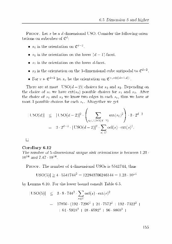
6 5 Dimension 5 and higher
Proof Let s be a d-dimensional USO Consider the following orien¬
tations on subcubes of £d
• so is the orientation on £d~2
• si is the orientation on the lower (d — l)-facet
• s2 is the orientation on the lower d-facet
• S3 is the orientation on the 3-dimensional cube antipodal to £d~2
• For v G £d~2 let sv be the orientation on £^ v®id-1 dil
There are at most | USO(d — 2)| choices for so and S3 Depending on
the choice of so we have ext(so) possible choices for si and S3 After
the choice of si and S3 we know two edges m each sv, thus we have at
most 3 possible choices for each sv Altogether we get
USO(d)| < |USO(d-2)|2 ( Y^ ext(so)2 ] 3 2
.s0eUSO(d-2)
d-2
= 3 2d~2 |USO(d-2)|2 ^ocl(s) ext( s)2sEU
D
Corollary 6.12
Tie number of 5-dimensional unique sink orientations is between 1 23
1014 and 7 47 1014
Proof The number of 4-dimensional USOs is 5541744, thus
|USO(5)| > 4 55417442 = 122843706246144 = 1 23 1014
by Lemma 6 10 For the lower bound consult Table 6 5
|USO(5)| < 3 8 7442 ^ocl(s) ext(sis)2sEU
21 O/l r7Cr7o2 1 1 no 70oo2
= 17856 (192 72962 + 24 75722 + 192 7322
+ 64 59182 + 48 65922 + 96 88682 +
155
6 Data
+ 48 • 87162 + 48 • 65922 + 8 • 105862 +
+ 24 • 78082) = 17856 • 41858776992
= 747430321969152 = 7.4743 • 1014.
D
Two different experiments indicate that the true value is closer to the
upper bound than to the lower bound. The first experiment is based on
an implementation of the Markov-chain introduced in Section 4.3. Let
p be the probability that a 5-dimensional USO is combed in direction 1.
As already observed in the proof of Lemma 6.10, the number of combed
orientations in USO(5) is
nc = 2 • | USO(4) |2 = 61421853123072.
Let n = | USO(5)|. Then nc = n-p. If we run the Markov-chain defined
by (4.6) n times and count the number nc of orientations combed in
direction 1, then we gethc—
->Pn
since the Markov-chain converges to the uniform distribution. Thus,
n
nc > n.
nc
The Markov-chain was implemented in C++. Starting with the uniform
5-dimensional orientation we receptively choose a label uniformly at
random from {1,... ,5}, calculate the phases along this label and flipeach phase with probability 1/2. An implementation can be found at
[38]. In an experiment with 109 iterations of the Markov-chain, where we
counted every 1000-st orientation, we observed nc = 9554 orientations
combed in direction 1. This gives an estimate of
h 10000014 , s
nc — = 661421853123072 = 6.4289 • 1014. 6.2
nc 9554v '
Although the numbers seem to converge, and appear reasonable as com¬
pared to our bounds, we want to point out that we have, in actual fact,no guarantee that the Markov-chain is already converging.
156

6 5 Dimension 5 and higher
The second experiment is using Lemma 6 9 Applied to the case
of dimension five, we have 1291 o-classes in dimension four For each
of them we have to calculate the number of phases combined with all
5541744 USOs of dimension four Even though this is not a trivial task,it is something a computer program can do An implementation of
this idea gave (after thee weeks calculation time) the following number
638560878292512 Although we do not have an actual proof that this is
the right result (the implementation could be wrong), it is quite likelythat this is the actual number of five-dimensional USOs
For higher dimensions, the upper bound from Lemma 6 11 fails, since
we do not have access to ext(s) The lower bound from Lemma 6 10
yields
|USO(6)| > 4 |USO(5)|2>64 | USO(4)|4 = 6 04 1028
|USO(7)| > 4 |USO(6)|2 >214 | USO(4)|8 = 1 46 1058
|USO(8)| > 4 |USO(7)|2 >230 | USO(4)|16 = 8 50 10116
Since the number of atoms m the universe is estimated to be between
1078 and 1079 This means that from dimension 8 on, any enumeration
of USO(d) will necessarily fail
157

6 Data
158

Bibliography
L. Adler and R. Saigal. Long monotone paths in abstract polytopes.Math. Oper. Res., 1:89-95, 1976.
N. Alon, J. Brück, J. Naor, M. Naor, and R. Roth. Construction
of asymptotically good, low-rate error-correcting codes through
pseudo-random graphs. IEEE Transactions on Information The¬
ory, 38:509-516, 1992.
N. Amenta and G. M. Ziegler. Deformed products and maxi¬
mal shadows of polytopes. Contemporary Mathematics, 223:57-90,1999.
M. Balmer and T. Szabo. Deterministic algorithms on unique sink
orientations of small dimension. Manuscript in preparation, 2003.
E. Behrends. Introduction to Markov Chains. Vieweg, Braun¬
schweig, 2002.
R. W. Cottle, J.-S. Pang, and R. E. Stone. The Linear Comple¬
mentary Problem. Academic Press, 1992.
G. Dantzig. Linear programming: The story about how it began.
Operations Research, 50(l):42-47, 2002.
M. Develin. LP-orientations of cubes and crosspolytopes. Advances
in Geometry, 2002. To appear.
B. Gärtner. A subexponential algorithm for abstract optimization
problems. SIAM Journal on Computing, 24:1018-1035, 1995.
B. Gärtner. Combinatorial linear programming: Geometry can
help. In Proc. 2nd Int. Workshop on Randomization and Approxi¬mation Techniques in Computer Science, volume 1518, pages 82-96,1998. Lecture Notes in Computer Science.
159

Bibliography
[11] B. Gärtner. Combinatorial structure in convex programs.
Manuscript, 2001.
[12] B. Gärtner. The random-facet simplex algorithm on combinatorial
cubes. Random Structure and Algorithms, 20(3):353-381, 2002.
[13] B. Gärtner. Strong LP-type problems. Manuscript, 2003.
[14] B. Gärtner, M. Henk, and G. M. Ziegler. Randomized simplex
algorithms on Klee-Minty cubes. Combinatorial, 18(3):349-372,1998.
[15] B. Gärtner and E. Welzl. Linear programming - randomization
and abstract frameworks. In Proc. 13th Annual Syrnp. on Theoret¬
ical Aspects of Computer Science (STAGS), pages 669-687. Lecture
Notes in Computer Science 1064, Springer, 1996.
[16] F. Granot and P. L. Hammer. On the use of boolean functions
in 0-1 programming. Methods of Operations Research, 34:154-184,1971.
[17] P. L. Hammer, B. Simeone, T. Liebling, and D. de Werra. From
linear separability to unimodality: a hierarchy of pseudo-booleanfunctions. SIAM J. Discrete Math., 1:174-184, 1988.
[18] K. W. Hoke. Completely unimodular numberings of a simple poly-
tope. Discrete Applied Mathematics, 20:69-81, 1988.
[19] F. Holt and V. Klee. A proof of the strict monotone 4-step conec-
ture. In J. Chazelle, J. B. Goodman, and R. Pollack, editors,Advances in Discrete and Computational Geometry, Contempo¬
rary Mathematics, pages 201-216. American Mathematical Society,1998.
[20] V. Kaibel. Bottom-top graphs. Manuscript,
http://www.ti.inf.ethz.ch/ew/workshops/01-lc/kaibel.html, 2001.
[21] G. Kalai. A subexponential randomized simplex algorithm. In
Proc. 2Jdh ACM Symposium on Theory of Computing, pages 475-
482, 1992.
160

Bibliography
[22] O. H. Keller. Über die lückenlose Erfüllung des Raumes mit
Würfeln. J. Reine Angew. Math., 163:231-248, 1930.
[23] L. G. Khachiyan. Polynomial algorithms in linear programming.U.S.S.R Comput. Math, and Math. Phys., 20:53-72, 1980.
[24] V. Klee and G. J. Minty. How good is the simplex algorithm. In
O. Shisha, editor, Inequalities - III. Academic Press Inc., New York
and London, 1972.
[25] J. C. Lagarias and P. W. Shor. Keller's cube-tiling conjecture is
false in high dimensions. Bulletin of the American Mathematical
Society, 27(2):279-283, 1992.
[26] J. Mackey. A cube tiling of dimension eight with no facetsharing.Discrete & Computational Geometry, 28:275-279, 2002.
[27] J. Matousek. The number of unique-sink orientations of the hyper-cube. Combinatorial, 2002. To appear.
[28] J. Matousek, M. Sharir, and E. Welzl. A subexponential bound for
linear programming. Algorithmica, 16:498-516, 1996.
[29] J. Matousek and T. Szabo. Random edge can be exponential on
abstract cubes. To appear in FOCS, 2004.
[30] J. Matousek and P. Valtr. personal communication, 2001.
[31] N. Megiddo and C. H. Papadimitriou. On total functions, existence
theorems and computational complexity. Theoretical Computer Sci¬
ence, 81:317-324, 1991.
[32] W. D. Morris. Distinguishing cube orientations arising from linear
programs. Submitted, 2002.
[33] W. D. Morris. Randomized principal pivot algorithms for P-matrix
linear complementarity problems. Mathematical Programming, Ser.
A(92):285-296, 2002.
[34] C. H. Papadimitriou. Computational complexity. Addison-Wesley,1994.
161

Bibliography
[35] A. L. Peressini, F. E. Sullivan, and J. J. Uhl. The Mathematics
of Nonlinear Programming. Undergraduate Texts in Mathematics.
Springer, 1988.
[36] O. Perron. Über die lückenlose Ausfüllung des n-dimensionalen
Raumes durch kongruente Würfel I & IL Math. Z., 47:1-26, 161—
180, 1940.
[37] H. Samelson, R. M. Thrall, and O. Wesler. A partition theorem
for Euclidean n-space. Proceedings of the American Mathematical
Society, 9:805-807.
[38] I. Schurr. The unique sink orientations in dimension 3 and 4.
http://www.inf.ethz.ch/personal/schurr/uso.
[39] I. Schurr and T. Szabo. Finding the sink takes some time. Discrete
Comput Geom, 31:627-642, 2004.
[40] A. Stickney and L. Watson. Digraph models of bard-type algo¬rithms for the linear complementary problem. Mathematics of Op¬erations Research, 3:322-333, 1978.
[41] S. Szabo. Cube tilings as contributions of algebra to geometry.
Beiträge zur Algebra und Geometrie, 34(l):63-75, 1993.
[42] T. Szabo and E. Welzl. Unique sink orientations of cubes. In Proc.
42nd IEEE Syrnp. on Foundations of Comput. Sei., pages 547-555,2000.
[43] N. Zadeh. What is the worst case behavior of the simplex algo¬rithm? Technical Report 27, Dept. Operation Research, Stanford,1980.
[44] G. M. Ziegler. Lectures on Polytopes. Number 152 in Graduate
texts in mathematics. Springer, 1995.
162
Curriculum Vitae
Ingo Andreas Schurr
born on March 12, 1972 in Baden-Baden, Germany.
1985-1992 high school in Baden Baden, Germany
Degree: Abitur
1993 2000 studies at Freie Universität Berlin, Germany
Major: Mathematics
Minor: Computer Science
Degree: Diplom
2000 2004 Ph.D. student at ETH Zürich, Switzerland